benchmarking banking sector efficiency across regional ... · pdf filebenchmarking banking...
TRANSCRIPT

Benchmarking Banking Sector Efficiency
Across Regional Blocks in Sub-Saharan Africa:
What Room for Policy?
François Boutin-Dufresne, Santiago Peña,
Oral Williams and Tomasz A. Zawisza
WP/13/51

© 2013 International Monetary Fund WP/13/51
IMF Working Paper
African Department
Benchmarking Banking Sector Efficiency Across Regional Blocks in Sub-Saharan Africa: What
Room for Policy?
Prepared by François Boutin-Dufresne, Santiago Peña, Oral Williams and
Tomasz A. Zawisza1
Authorized for distribution by Paolo Mauro
February 2013
Abstract
This paper examines the determinants of net interest margins in four regional blocks in
Sub-Saharan Africa and one comparator block in the Eastern Caribbean. Using bank-level
data, we find that countries with a high level of operating costs, a high ratio of equity to
total assets and high treasury bill interest rates have higher net interest margins. Moreover,
high operating costs are associated with low measures of institutional quality and a small
size of bank operations. We find support for the view that market structure is also partly
responsible for high net interest margins in Sub-Saharan Africa. If interpreted causally,
high operating costs and a high ratio of equity to total assets and, indirectly, institutional
factors such as the rule of law, are the most important factors in accounting for high
interest margins in the East African Community, relative to other regions.
JEL Classification Numbers: G14, G21, G28, E44, E52
Keywords: Financial intermediation efficiency, net interest margins, economies of scale,
institutions.
Authors e-mail addresses: [email protected]; [email protected]; [email protected] and
1 This study was conducted when Mr. Zawisza was a summer intern in the African Department. The authors thank
Adolfo Barajas, Jorge Canales-Kriljenko Ralph Chami, Anne-Marie Gulde, Heiko Hesse, David Marston, Tigran
Poghosyan, and participants from the African Department‘s Financial Sector Network and those from the Money and
Capital Markets Seminar series who provided constructive comments. All remaining errors accrue to the authors.
This Working Paper should not be reported as representing the views of the IMF.
The views expressed in this Working Paper are those of the author(s) and do not necessarily
represent those of the IMF or IMF policy. Working Papers describe research in progress by the
author(s) and are published to elicit comments and to further debate.

2
Contents Page
I. Introduction ............................................................................................................................4
II. Literature Review ..................................................................................................................5
III. Evolution of Net interest margins (1997–2011) ..................................................................6
IV. Empirical Strategy .............................................................................................................10
A. Econometric model .................................................................................................10
B. Data .........................................................................................................................12
V. Results .................................................................................................................................13
A. Pooled OLS .............................................................................................................14
B. Fixed Effects and System GMM .............................................................................17
VI. Concluding Remarks .........................................................................................................23
Appendix I ...............................................................................................................................27
Measuring Market Competition ...................................................................................27
Appendix II ..............................................................................................................................28
Tables
2. Variable definitions and sources. .........................................................................................12
3. Determinants of net interest margins (pooled OLS) ............................................................14
4. Determinants of operating costs (pooled OLS) ...................................................................15
5. Determinants of operating costs regression - additional controls (pooled ...........................16
7. Role of alternative measures of market structure (system GMM ........................................20
8. Economic significance of net interest margin determinants for whole................................21
9. Economic significance of operating cost determinants (indirect impact on ........................22
10. Regional comparison using 2011 values and system GMM estimates ..............................22
Figures
1. Evolution of Net Interest Margins Across Regions ...............................................................8
2. NIMs and Equity-to-Asset Ratio ...........................................................................................9

3
I. INTRODUCTION
Channeling funds from savers to investors is one of the key functions of financial
intermediaries. One measure of the efficiency with which banks perform this function is the
net interest margin (NIM), which is defined in this study as the value of a bank‘s net interest
revenue as a share of its total assets.2 Within Sub-Saharan Africa (SSA), NIMs are on
average considerably higher than in most developed economies, raising the question of
whether inefficiencies in the channeling of finance have been a constraint to growth. In
recent years, certain countries, such as those in the East African Community (EAC), seem to
have experienced a sustained downward trend in margins, whereas other regions have seen
margins grow or fluctuate around a trend.
To the extent high NIMs are may be considered as a signal of inefficiency, understanding
their determinants is a key priority for policymakers willing to increase the potential for
growth linked to a more efficient financial system.3 However, high margins can in principle
arise for a multitude of reasons. Beck and Hesse (2009) document the various possible
explanations and group them under four main hypotheses. According to the risk-based
hypothesis, informational imperfections in the relationship between banks and borrowers
generate costs. These costs may stem from the inability to ascertain the borrowers‘
creditworthiness, which can lead to adverse selection and the pricing of safer borrowers out
of the market. At the same time, lack of information about a borrower‘s behavior may lead to
moral hazard. In both of these cases, information asymmetries may lead banks to charge
higher margins as compensation for risk. A second view, the small financial system
hypothesis, identifies the cause of high NIMs with the fixed costs of providing financial
services, such as those associated with setting up branches. The presence of fixed costs may
make it difficult for small financial systems to take advantage of scale economies, requiring
high margins to compensate for high average costs (Bottomley, 1963). The third view, the
market structure hypothesis, seeks to explain high margins through imperfectly competitive
banking behavior. High NIMs according to this view reflect high economic rents earned by
banks in an environment of low competition. Finally, the macroeconomic hypothesis stresses
the role of the exchange rate, interest rate, and real economy fluctuations. This view attempts
to capture several possible causal mechanisms from macroeconomic factors to high NIMs:
for instance, high domestic interest rates may reflect large macroeconomic risks, imposing
additional costs on banks and, again, leading them to charge high NIMs as a result.
The four different hypotheses have very different policy implications. For instance, if the
fixed costs of lending are the underlying cause of high margins, efforts to promote
2 A distinction must be made between net interest margins and the average banking spread—the difference
between ex-ante contracted lending and deposit interest rates. It is possible for net interest margins to be low
and ex ante spreads to be high, for instance if there is widespread default among borrowers. We leave the
examination of the link between NIMs and spreads for further work, and hence about the extent to which the
conclusions of this paper apply more generally.
3 High net interest margins are also correlated with low financial depth, making NIMs a relevant indicator for
the IMFs recent focus on financial deepening in developing countries.

4
competition among banks are unlikely to be fruitful. On the other hand, if large asymmetries
of information between banks and borrowers create a high degree of risk in lending,
stabilizing the macroeconomy will not eliminate the underlying risk driving high margins.
Reducing information asymmetries through credit bureaus, or reducing the costs of such
asymmetries through improved asset recovery in the face of default, would be more suitable
strategies. Thus, it is critical to determine which of the hypothesis are supported by the data,
and which drivers are the main determinants of NIMs.
By investigating the above-mentioned hypotheses together, this study seeks to assess their
relative contribution to NIMs across several regional groupings. Our choice of explanatory
variables is guided by each of the four hypotheses. We therefore include measures of lending
risk, monopolistic rents, economies of scale and business-cycle movements as possible
explanatory variables for NIMs. Additionally, our paper adopts a regional perspective. We
attempt to explain the observed patterns of cross-sectional and time-series variation in NIMs
among four regional groupings in SSA. These groupings share common institutional
characteristics, in that they either involve a common currency and customs union, or state
these as central goals.4 The SSA regions investigated are the EAC, the West African
Economic and Monetary Union (WAEMU), the Central African Economic and Monetary
Community (CEMAC), as well as the South African Customs Union (SACU).5 In addition to
these SSA regional associations, we include the Eastern Caribbean Currency Union (ECCU)
as a comparator, as it performs similarly according to key measures and enjoys similar
institutional arrangements.6
The paper uncovers several important findings. First, we find strong evidence that bank
operating costs and equity-to-capital ratios are both statistically and economically significant
determinants of NIMs in all regions. Moreover, there is evidence that poor institutional
quality indirectly influences NIMs through higher operating costs. This result is consistent
with the view that poor regulatory quality and rule of law cause banks to engage in costly
credit appraisals and monitoring, as suggested by Honohan and Beck (2007). Additionally,
operating costs are strongly and inversely related to the size of the loan portfolio, suggesting
that fixed costs to lending are non-trivial in our sample, creating scope for banks with larger
loan portfolios to exploit economies of scale. Taken together, our results are consistent with
4 Two out of the four, namely CEMAC and WAEMU, have formally adopted a currency union, whereas the
EAC state a currency union as a long-term objective. SACU and WAEMU operate a customs union while the
EAC and CEMAC have stated a customs union to be a long-term goal.
5 The East African Community (EAC) consists of Burundi, Kenya, Rwanda, Tanzania and Uganda; the
Economic and Monetary Community of Central Africa (CEMAC) consists of Cameroon, the Central African
Republic (CAR), Equatorial Guinea, Republic of Congo and Gabon; the East Caribbean Currency Union
(ECCU) consists of Antigua and Barbuda, Dominica, Grenada, St Kitts and Nevis, St Lucia and St Vincent and
the Grenadines; the West African Economic and Monetary Union (WAEMU) consists of Benin, Burkina Faso,
Cote d‘Ivoire, Guinea-Bissau, Mali, Niger, Senegal and Togo, and the Southern African Customs Union
(SACU), consisting of Botswana, Lesotho, Namibia, South Africa and Swaziland.
6 Specifically, ECCU operates a currency union, with a currency board and the members‘ currency pegged to
the dollar at a fixed rate.

5
both the risk-based and small financial system views, namely that the small nature of the
African financial systems and risk factors, amplified by the inefficiency of the judicial
system, are key determinants of high margins.
The structure of the paper is organized as follows. Section II presents a brief review of the
literature, provides a motivation for our choice of explanatory variables, and situates the
contribution of our paper. Section III provides stylized facts regarding the evolution of NIMs
and their various accounting components between 1997 and 2011 in the regions under study,
suggesting some preliminary hypotheses for our econometric analysis. Section IV outlines
our econometric strategy to test the relative importance of the four hypotheses outlined by
Beck and Hesse (2009). Our estimation results are presented in Section V. Finally Section VI
concludes with a discussion of policy recommendations and areas for future work.
II. LITERATURE REVIEW
A large body of empirical work has examined the determinants of NIMs in developed
economies, with a smaller but growing literature examining NIMs in Emerging Markets
(EMs) and Low Income Countries (LICs). However, only a few firm conclusions appear to
emerge. There is some consensus on the role of macroeconomic and bank-specific variables
in determining NIMs, but evidence is less clear cut for the role of institutions and the degree
of bank competition. We provide a brief summary, focusing on findings regarding the role of
macroeconomic, market-structure, institutional and bank-specific variables.
Macroeconomic environment: The dealership model of Ho and Saunders (1981) has
influenced early work on NIMs whereby these rise with the variance of interest rates
in the face of intermediation risks. This hypothesis was corroborated by Maudos and
de Guevara (2004) who employed the dealership model and found that with
macroeconomic variables in the form of interest-rate volatility played a significant
role. Inflation and high treasury bill rates have also been found to be positively
correlated with bank spreads (Hoonahan, 2003, Ahokpossi, 2012; Poghosyan, 2010).
Degree of bank competition: Standard theory predicts more intense competition to
yield lower spreads.7 However, the empirical evidence has been mixed. One difficulty
is that the proxies for market structure used in the literature are not always
comparable, with market concentration indicators used by some of the authors
appearing fragile. Nevertheless, Poghysan (2010) and Martinez-Peria and Moody
(2004) find a significant effect of market concentration.
Bank specific factors: Building on the dealership model of Ho and Sounders (1981),
many studies have found a role of bank specific factors (Beck and Hesse, 2009;
Poghysan, 2010; Gelos, 2009). Higher operating costs were found to be positively
7 However, some recent papers have argued imperfect competition may encourage efficient lending (e.g.
Petersen and Rajan, 1995), emphasizing the need for establishing the interplay between NIMs and market
competition empirically.
6
associated with higher NIMs. Depending on their strategy, some banks may rely more
on fee income which negatively affect NIMs. Higher non-performing loans could also
lead to higher margins through higher risk premia. As Demirguc-Kunt, Laeven and
Levine, (2004) have demonstrated, capitalization could affect funding costs and as a
result NIMs.
Institutional setting: Other studies have attempted to explore the role of institutions
and found that they have a significant effect on NIMs (Demirguc-Kunt, Laeven and
Levine, 2004; Poghosyan, 2012). An institutional setting that permits loan recovery
and preservation of creditor rights through strong legal environment are expected to
lower NIMs.
Findings for SSA: The seminal work by Honohan and Beck (2007) provides a
discussion of the challenges facing the banking sector in the region as a result of
volatile macroeconomic environment and a small size of most financial systems.
Beck and Hesse (2009) explored the four sets of hypotheses for high margins
discussed above and find a role for macroeconomic variables. They find that faster
GDP growth, rising inflation and increasing treasury bill rates to be associated with
higher margins, whereas lower spreads are linked to better institutions and larger
balance sheets. They also found strong evidence for risk-based approach and some
evidence for macroeconomic views, but little evidence for the market structure view.
For a large sample of banks in SSA, Ahokpossi (2012) finds an important role for
lending risk, interest rate risk, bank equity and non-interest activity. Among
macroeconomic variables, inflation appears to be statistically significant, with
non-linear effects.
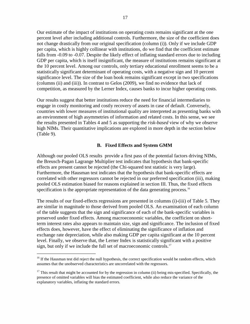
III. EVOLUTION OF NET INTEREST MARGINS (1997–2011)
In Figure 1, we summarize the cross-sectional and time-series patterns of NIMs in our
sample of five regions, during 1997– 2011. We define NIMs for bank i in country c at time t
as follows:
(1)
where total interest revenue , total interest expense and total assets are
taken from the income statement of the bank for year t. We begin with a discussion of
differences in levels of NIMs in the sample, and follow with a brief overview of trends.
The difference between interest received and interest paid by the bank goes towards
personnel costs and other non-interest operating costs , provisions for loan losses
, as well as contributing to profits . All of these items are related by the accounting
identity:
(2)

7
On dividing by total assets, and solving for , we can use (2) to
express NIMs as the following five components profit before tax, loan-loss provisions,
non-interest income, operating costs and an error term, all normalized by total assets8. Thus,
in this section, we complement our account of the evolution of NIMs in the five regions with
the evolution of their various components. Figure 1 examines the evolution of NIMs between
1997–2011 in the five regions under investigation and illustrates considerable heterogeneity.
Throughout 1997–2011, the EAC had the highest margin levels of all the regions. On
average, these were over 2 percentage points greater than in the next-highest region,
WAEMU. By 2011, CEMAC, ECCU and WAEMU had similar levels of margins, although
the regions faced considerable heterogeneity in 1997. By 2011 SACU had the lowest margins
of all five regions at 2.72 percentage points, with the EAC still having the highest NIMs at
above 6 percentage points. In ECCU, margins remained fairly constant over the period
1997-2011, but oscillating somewhat between 3.7 and 2.5 percentage points.
The trends in NIMs have also been quite heterogeneous across the regions. There has been a
sustained decline in margins in the EAC between 2001 and 2008. In this period, margins fell
from a high of 7.7 percentage points in 2001 to 5.7 in 2008, before rising somewhat to 6.2
from 2009 to 2011. Figure 1 illustrates that declining operating costs and loan-loss provisions
were associated to large extent with this trend. For instance, loan-loss provisions accounted
for 2.7 percentage points of the margin in the EAC in 2002, but only 0.4 percentage points in
2011. In the same period, operating costs fell from 6.9 percentage points in the EAC to
5.7 percentage points. The WAEMU region also experienced a sustained decline in margins,
from 5.2 in 1998 to 3.5 percentage points in 2011, but in contrast to the EAC this was not
associated with a decline in operating costs. Rather, for WAEMU, this trend was associated
with falling loan-loss provisions and rising non-interest income.
8 Unlike in Randall (1998), reserves do not enter our decomposition. This is because we use a different
definition of margins. As in Beck and Hesse (2009), we define them as net interest revenue over total assets.
Randall, on the other hand, defines net interest margins as total interest revenue/interest-bearing assets minus
total interest expense/funding. This generates an additional term when normalizing by total assets. The error
term in Table 1 stems from the inclusion of non-standard expenses and income in the income statement in
BankScope; however, it is negligible and we do not focus on it in the analysis.

8
Figure 1. Evolution of Net Interest Margins Across Regions
Both CEMAC and SACU experienced considerable volatility in NIMs between 1997 and
2011. CEMAC initially had low NIMs (1.3 percentage points in 1998), coupled with very
high levels of non-interest income (equivalent to 9.4 percentage points). This may be related
to the structural differences due to the dominance of oil firms in the region, and the heavy
-10
-8
-6
-4
-2
0
2
4
6
8
10
12
14
1997 1999 2001 2003 2005 2007 2009 2011
EAC
Error
Minus non-interest
incomeProfit before tax
Loan-loss provisions
Operating costs
-10
-8
-6
-4
-2
0
2
4
6
8
10
12
14
1997 2004 2011
CEMAC
Error
Minus non-interest
incomeProfit before tax
Loan-loss provisions
Operating costs
-10
-8
-6
-4
-2
0
2
4
6
8
10
12
14
1997 1999 2001 2003 2005 2007 2009 2011
ECCU
Error
Minus non-interest incomeProfit before tax
Loan-loss provisionsOperating costs
Margin
-10
-8
-6
-4
-2
0
2
4
6
8
10
12
14
1997 2004 2011
WAEMU
Error
Minus non-interest
incomeProfit before tax
Loan-loss provisions
Operating costs
-10
-8
-6
-4
-2
0
2
4
6
8
10
12
14
1997 1999 2001 2003 2005 2007 2009 2011
SACU
Error
Minus non-interest incomeProfit before tax
Loan-loss provisionsOperating costs

9
reliance of banks on lending to firms with government contracts. After a period of
considerable volatility, margins rose to 3.6 percent in 2011. SACU similarly experienced
considerable fluctuations in NIMs between 1997 and 2004, which coincided with large
changes in operating costs. This volatility may be due to the considerable structural change in
the South African banking sector comprising a number of mergers and acquisitions.
Among the variables in the decomposition, operating costs and loan-loss provisions seem to
have been associated most closely with movements in NIMs across the regions. The data also
seems to suggest that operating costs both move closely with margins and explain long-run
differences. A decline in loan-loss provisions appears to have been associated with declines
in margins in the EAC and WAEMU, but to have also been a trend present in all five regions.
Over the whole period, operating costs were by far the largest contributor to margins in all
regions except CEMAC, where it accounted for between 41 (SACU) and 46 percent (ECCU)
of the margin on average.
A further variable which seems to be closely correlated with NIMs, but is not included in the
decompositions above, is the ratio of equity to total assets. The relationship between NIMs
and the log of the equity-to-asset ratio in repeated cross-sections in our sample is presented in
Figure 2 above. The correlation presented here, with an R-squared of 0.125, presents a strong
prima-facie case that equity may be important in explaining NIMs in our sample.

10
IV. EMPIRICAL STRATEGY
Building on the stylized facts derived from the data, we test the four hypotheses outlined in
the introduction, using three alternative econometric estimation techniques: pooled OLS, the
inclusion of unobserved (time constant) bank characteristics using fixed effects and serial
dependence in NIMs using system GMM.
A. Econometric model
The following panel data specification encompasses three empirical models
1 ' 'ict ict ict ct ic t icty y x z (3)
where icty represents the bank net interest margin for bank i, country c and time t, ictx denotes
the vector of bank-specific explanatory variables described in section II., whilectz is the
vector of country-specific macroeconomic, institutional and market-structure variables. ic is
an unobserved time-constant bank-specific effect; t is the time-specific effect9 and ict is the
error term capturing all other omitted factors. We iteratively expand our specification to
include, sequentially, bank-specific, market-structure, macroeconomic and institutional
variables.
Following Ho and Saunders (1981) model, we include operating costs, loan-loss provisions,
non-interest income, liquid assets, equity and the size of the loan book as bank-level
explanatory variables. For completeness, both the Lerner and HHI indices are used as
measures of market structure, and their derivation is presented in Appendix I. Inflation, the
exchange rate and GDP per capita are considered among the macroeconomic factors which
may influence NIMs. Honohan and Beck (2007) also suggest that high wholesale interest
rates, proxied by the treasury bill rate and central bank rate, reflect currency and other
macroeconomic uncertainty, as well as the government demand for loanable funds.
Institutional variables encompass a range of governance indicators, which we capture in our
preferred specification by a composite index, explained further in Section B below.
Pooled OLS, which comprises our initial specification, is both unbiased and efficient if the
bank-specific effects are zero for all i and all t, and . However, in the presence of bank
fixed effects, such as time-constant differences in managerial quality, OLS is inappropriate.
Even if the bank fixed effects are uncorrelated with the regressors, the estimator will be
inefficient; if such correlation does exist, the OLS estimates will be biased. Fixed effects is
the appropriate estimation technique if unobserved bank characteristics are both present and
9 All of our models are estimated with the full set of time fixed effects, which capture common shocks to
(common trends in) the net interest margins for all banks in all regions. Also, all of our specifications use robust
standard errors.

11
correlated with the other control variables, and the assumption of strict exogeneity holds.10
As will be seen in the next section, we do find that unobserved bank characteristics matter.
Nevertheless, we believe it is important to include our pooled OLS results. Firstly, fixed
effects have limited power to identify the effects of variables which are persistent over time,
as the demeaning operation reduces variation, resulting in a loss of precision. This is
particularly problematic for our measures of institutions, which are very persistent over
time.11 Moreover, in the presence of measurement error and persistent independent variables,
fixed effects can result in considerable attenuation bias (Deaton, 1995).
If both bank fixed effects are non-zero and are correlated with the regressors, and
0 , i.e. the true model has a lagged dependent variable, Nickell (1981) demonstrates that
the strict exogeneity assumption fails and, consequently, fixed effects is biased. In our case,
we cannot determine a priori that banks might smooth NIMs over time, for instance due to
reasons similar to those often cited to explain standard price persistence. If this is the case, it
is either appropriate to circumvent the bias either by using the difference GMM estimator
proposed by Arellano and Bond (1991), or the system GMM estimator proposed by Arellano
and Bover (1995) and Blundell and Bond (1998). In this paper, we will opt for the system
GMM estimator, as it resolves some of the small-sample biases and imprecision of the
difference GMM estimator without very strong assumptions (Baltagi, 2005). This estimation
technique is appropriate under the assumption that there is no correlation between the
differences of the variables and the bank-specific effects.
We remain agnostic about whether fixed effects or system GMM is the appropriate
estimation technique in our context. As discussed by Angrist and Pischke (2009), while the
dynamic panel GMM model does not nest the fixed effects model, or vice versa, the two have
a useful bounding property on the causal effects of interest.12 In our results section, we will
consider the two estimation techniques to give bounds on the likely magnitude of the
parameters of interest.
10
In the context of our model, the assumption of strict exogeneity amounts to the independent variables being
uncorrelated with the error terms in all periods, i.e. [( ' , ' ) ' ]ict ct icsE e x z 0 for all t,s = 1,2,…,T. As discussed
in the text, the assumption fails if the lagged dependent variable features among the regressors.
11 For this reason, when we regress operating costs on institutional variables, the size of operations and various
controls to test the hypothesis that economies of scale and institutions impact net interest margins through the
operating cost channel, we will resort purely to pooled OLS methods.
12 In particular, if the dynamic specification is correct, but we mistakenly use fixed effects, estimates of a
positive effect will be too large. On the other hand, if the fixed effects specification is correct, but we
mistakenly estimate an equation with the lagged dependent variable, estimates of a positive effect will tend to
be too small.

12
B. Data
In order to exploit the variation in the data as far as possible, we chose to keep the analysis at
the level of individual banks. All bank-specific data were obtained from the BankScope
database supplied by Bureau Van Dijk. Table 1 provides a summary of all variables and their
sources. Macroeconomic variables were sourced from the World Economic Outlook of the
International Monetary Fund. The World Bank‘s World Governance Indicators (WGI)
outlined in Kaufman et al. (2005) was the source of information on institutions.
Table 1: Variable Definitions And Sources
Our original sample of banks for the five regions in BankScope consisted of 400 banks in 30
countries over the period 1997-2011. However, we eliminated microfinance institutions and
holding companies for other banks in the sample, and all banks which had fewer than four
consecutive yearly observations. 13 We also eliminated outliers by removing all banks in the
top and bottom percentiles of the distributions of bank-specific variables, with the exception
of the size of the loan book. This yielded a final sample of 213 banks, as the basis for an
unbalanced panel.
13
The presumption being that microfinance institutions do not necessarily follow the same model of behavior as
commercial banks. MFIs were identified using the Microfinance Information exchange database, found on
http://www.themix.org/. The Stanford Bank in Antigua and Barbuda was also dropped, as it altered the results
for ECCU significantly given its large balance sheet and the non-standard nature of operations.
Variable Measure Source
Bank-specific Variables
Net interest margin Ratio of total interest revenues net of total interest expenses to total assets BankScope
Operating costs Ratio of total operating expenses to total assets (log) BankScope
Equity Ratio of total equity to total assets (log) BankScope
Loan-loss provisions Ratio of loan loss provisions to total assets (log) BankScope
Liquidit assets Ratio of liquid assets to total assets BankScope
Size of operations Logarithm of total loans BankScope
Non-interest income Ratio of non-interest income to total assets BankScope
Market competition
Lerner Index See Appendix I for definition Author calculations
HHI (Deposits) See Appendix I for definition BankScope
HHI (Assets) See Appendix I for definition BankScope
Governance
WGI Voice and Accountability See Kaufman et al. (2011) for definition Kaufman et al. (2011)
WGI Political Stability See Kaufman et al. (2011) for definition Kaufman et al. (2011)
WGI Government Effectiveness See Kaufman et al. (2011) for definition Kaufman et al. (2011)
WGI Regulatory Quality See Kaufman et al. (2011) for definition Kaufman et al. (2011)
WGI Rule of Law See Kaufman et al. (2011) for definition Kaufman et al. (2011)
WGI Control of Corruption See Kaufman et al. (2011) for definition Kaufman et al. (2011)
WGI Composite Synthetic measure based on first principal component of governance indicators Author calculations
Macroeconomic
GDP per capita GDP per capita in USD World Economic Outlook
Exchange rate % change in USD exchange rate World Economic Outlook
Inflation % change in CPI World Economic Outlook
Treasury Bill Interest rate on 3-month Treasury Bill paper* World Economic Outlook
Notes: (*) Central bank discount rates used where Treasury Bill rates not available.

13
We perform a number of transformations to the variables. Operating costs, equity-to-asset
ratios, loans and the loan loss provisions are all entered in logs. As the six measures of
institutions in the WGI are highly collinear, a summary index of institutions using principal
components analysis was constructed, with weights derived from the first principal
component.
V. RESULTS
In this section, we present our estimates of the various hypothesized determinants of
net interest margins for banks in the five regional groupings during 1997–2011. In Table 2
column (i), the coefficients on operating costs, equity, loan size and loan-impairment charges
were positive and statistically significant. The coefficient on non-interest activity was
negative, as expected, and statistically significant at the one percent level. Among bank-
specific variables, we only did not find the ratio of liquid to total assets to be statistically
significant. In the more general specifications in columns (ii) and (iii), we observe that the
bank specific variables are robust to controlling for market structure. Aside from the
coefficient on operating costs, which falls by about 24 percent in magnitude, the coefficients
remain very similar.
Our market competition measure proxied by the Lerner index (column (ii)) is
significant at the five percent level. Once we control for macroeconomic variables (column
(iii)), the statistical significance of the Lerner Index rises to one percent. The coefficient also
rises by over 50 percent, suggesting downward omitted-variable bias in column (ii). Again,
we observe that the sign and significance of the coefficients on bank-specific variables are
robust to the inclusion of macroeconomic variables. Of the macroeconomic variables, short-
term interest rates and inflation are significant with a positive sign at the two and one percent
levels respectively, while exchange rate depreciation is significant with a negative sign at the
one percent level (i.e. exchange rate depreciation lowers NIMs), giving some prima facie
support regarding the macroeconomic view. The result that depreciation is associated with
lower margins runs somewhat counter to our expectations but, as illustrated later, this result
is not robust to controlling for fixed effects and serial correlation. Perhaps surprisingly, GDP
per capita is not significant at any level.
Although the results are robust after controlling for institutional variables, (columns (iv) to
(x)) institutions are not statistically significant. As indicated earlier, there is a high degree of
collinearity among the various measures of institutions. Despite considering separately the
effect of alternative measures of institutions, including a synthetic measure based on
principal components analysis (column (x)), none of these yield results that are statistically
significant.

14
A. Pooled OLS
Table 2: Determinants Of Net Interest Margins (pooled OLS)
As this result runs counter to those of Demirguc-Kunt et al., (2004) who find a direct effect,
we investigate the possibility that institutions may impact NIMs indirectly through operating
costs. The role of institutions is therefore explored through an auxiliary pooled OLS
regression (Table 3) with operating costs as the dependent variable, and the size of loans,
non-performing loans, the Lerner Index and World Governance Indicators as controls. The
inclusion of the Lerner Index permits the testing of the hypothesis that uncompetitive
markets have higher levels of operating costs relative to competitive markets. The results
suggest that operating costs decline with all five different measures of institutions by
Kaufman et al., with levels of significance between one and 10 percent. In our preferred
Net interest margin (i) (ii) (iii) (iv) (v) (vi) (vii) (viii) (ix) (x)
Operating costs/assets (log) 3.054*** 2.331*** 2.250*** 2.239*** 2.235*** 2.244***2.244*** 2.234*** 2.241*** 2.242***[8.701] [9.005] [9.068] [8.964] [8.956] [8.957] [9.020] [8.980] [8.946] [8.979]
Equity/assets (log) 1.354*** 1.501*** 1.310*** 1.295*** 1.274*** 1.289*** 1.291*** 1.293*** 1.306*** 1.290***
[5.313] [6.215] [6.309] [6.333] [5.885] [6.309] [6.417] [6.334] [6.237] [6.232]
Loans (log) 0.164** 0.183** 0.225*** 0.227*** 0.223*** 0.223*** 0.226*** 0.226*** 0.229*** 0.225***
[2.008] [2.195] [2.964] [2.980] [2.939] [2.942] [3.001] [2.941] [2.966] [2.960]
Liquid/total assets 0.0123** -0.00053 -0.00613 -0.00564 -0.00528 -0 -0.00554 -0.00547 -0.00492 -0.00552
[2.007] [-0.0941] [-1.060] [-0.972] [-0.903] [-0.948] [-0.949] [-0.943] [-0.865] [-0.954]
Loan impairment charge/assets (log) 0.252*** 0.263*** 0.241*** 0.243*** 0.241*** 0.246*** 0.244*** 0.249*** 0.250*** 0.244***
[3.420] [3.657] [3.436] [3.634] [3.579] [3.632] [3.598] [3.693] [3.669] [3.601]
Non-interest activity/assets -0.424*** -0.321*** -0.281*** -0.292*** -0.289***-0.287***-0.288*** -0.284*** -0.287*** -0.288***
[-6.332] [-5.869] [-5.380] [-5.596] [-5.555] [-5.475] [-5.463] [-5.429] [-5.483] [-5.498]
Lerner Index 0.562** 1.230*** 1.131*** 1.199*** 1.229*** 1.193*** 1.242*** 1.268*** 1.197***
[2.076] [3.867] [3.371] [3.827] [3.620] [3.632] [3.756] [3.713] [3.546]
Inflation 0.0350** 0.0350** 0.0307* 0.0341**0.0348** 0.0364** 0.0362** 0.0347**
[2.174] [2.120] [1.870] [2.081] [2.156] [2.212] [2.223] [2.107]
T-Bill rate 0.125*** 0.120*** 0.122*** 0.121*** 0.122*** 0.122*** 0.122*** 0.122***
[4.952] [4.486] [4.655] [4.729] [4.732] [4.737] [4.761] [4.707]
USD exchange rate (% change) -0.0164** -0.0149** -0.0147**-0.0149**-0.0150** -0.0143** -0.0139** -0.0149**
[-2.558] [-2.307] [-2.300] [-2.265] [-2.253] [-2.167] [-2.076] [-2.277]
GDP per capita (log) 2.81E-05 3.52E-05 4.53E-05 0 2.74E-05 2.93E-06 -4.1E-06 2.59E-05
[0.648] [0.813] [1.051] [0.378] [0.587] [0.0625] [-0.0869] [0.566]
WGI Voice and Accountability -0.115
[-0.739]
WGI Political Stability -0.11
[-0.779]
WGI Government Effectiveness 0.07
[0.294]
WGI Regulatory Quality -0.0169
[-0.0592]
WGI Rule of Law 0.175
[0.725]
WGI Control of Corruption 0.197
[0.812]
WGI Composite -0.00048
[-0.00439]
Constant -2.076** -1.272 -3.020*** -2.920*** -2.872***-2.845***-2.921*** -2.787*** -2.845*** -2.907***
[-2.528] [-1.546] [-3.585] [-3.494] [-3.353] [-3.552] [-3.686] [-3.504] [-3.519] [-3.615]
Observations 1524 1400 1399 1320 1320 1320 1320 1320 1320 1320
R-squared 0.417 0.419 0.474 0.467 0.467 0.47 0.466 0.467 0.467 0.466
No. of banks 213 210 210 209 209 209 209 209 209 209
Notes: We use standard errors which are robust to rabitrary heteroskedasticity and clustering at the bank level. Year dummies are included in all
regressions. t-statistics are presented in brackets. The levels of significance are denoted as follows: *** p<0.01, ** p<0.05, * p<0.1

15
specification (viii), with the composite measure of institutions, institutions are statistically
significant at the one percent level with a coefficient of -0.09. This is suggestive of the
importance of institutional factors for the costs of intermediation.
Of the five measures of institutions, Voice and Accountability, Rule of Law and Control of
Corruption measures result in the lowest standard errors, suggesting the strongest relevance
for operating costs. Our preferred measure—the composite index of governance variables—
is also highly statistically significant. The results are consistent with anecdotal evidence that
the poor institutional climate in which SSA banks operate causes them to engage in costly
monitoring or screening which, in turn, leads to higher NIMs.14 The inclusion of the size of
the loan book facilitates the testing of the hypothesis that average operating costs per asset
decline with an increase in the size of loans (e.g. due to fixed costs of intermediation), thus
allowing us to test the small financial system hypothesis. In line with the small financial
system view, operating costs are negatively associated with a larger loan portfolio, with a
coefficient around -0.06.
Table 3: Determinants Of Operating Costs (pooled OLS)
14
Our results corroborate the findings of Demirguc-Kunt, Laeven and Levine (2004), who also find governance
to be important for bank operating costs.
Operating costs (log) (i) (ii) (iii) (iv) (v) (vi) (vii)
Size of operations (log) -0.0584*** -0.0661*** -0.0636*** -0.0651*** -0.0640*** -0.0642*** -0.0609***
[-2.704] [-3.269] [-3.101] [-3.049] [-3.065] [-3.097] [-2.942]
Non-performing Loans (log) 0.0198 0.0184 0.0152 0.019 0.0143 0.0115 0.0142
[1.044] [0.951] [0.779] [0.978] [0.752] [0.608] [0.741]
Lerner Index 0.0522 0.0662 -0.0579 0.0359 0.0394 0.00961 -0.0199
[0.478] [0.549] [-0.483] [0.312] [0.346] [0.0855] [-0.169]
WGI Voice and Accountability -0.151***
[-3.030]
WGI Political Stability -0.114***
[-2.815]
WGI Government Effectiveness -0.219***
[-3.470]
WGI Regulatory Quality -0.162*
[-1.722]
WGI Rule of Law -0.159***
[-2.617]
WGI Control of Corruption -0.155***
[-2.932]
WGI Composite -0.0917***
[-3.555]
Constant 1.775*** 1.801*** 1.759*** 1.812*** 1.768*** 1.782*** 1.749***
[14.60] [15.50] [14.54] [14.81] [14.12] [14.54] [14.38]
R -squared 0.148 0.145 0.147 0.125 0.138 0.141 0.153
Observations 1011 965 965 965 965 965 965
Number of banks 170 170 170 170 170 170 170
Notes: Robust t-statistics in brackets. *** p<0.01, ** p<0.05, * p<0.1

16
Table 4: Determinants of Operating Costs Regression - Additional Controls (pooled OLS)
Table 4 tests the robustness of the above findings to omitted variables. In so doing,
country-specific variables which might also tend to reduce operating costs, but which may be
correlated with our measure of institutions, such as enrollment rates in secondary education
(column (ii)) and enrollment rates in tertiary education (column (iii)) are explored. The
underlying hypothesis is that low rates of enrollment will impose higher labor costs for
banks, which anecdotally seem to recruit workers with higher levels of skills. Additionally, a
measure of infrastructure (column (iv)), proxied by the number of telephone lines per capita
in a given year is included.15 Finally, as a general proxy of potential omitted variables we
include GDP per capita in column (v).
15
Our measures of secondary and tertiary enrollment, as well as infrastructure measures, are sourced from the
World Bank‘s World Development Indicators database.
Operating costs (log) (i) (ii) (iii) (iv) (v)
WGI Composite -0.0917*** -0.100*** -0.0794*** -0.0842*** -0.0692*
[-3.555] [-3.803] [-3.055] [-2.685] [-1.851]
Size of operations (log) -0.0609*** -0.0187 -0.0331 -0.0589*** -0.0588***
[-2.942] [-0.718] [-1.107] [-2.810] [-2.830]
Non-performing Loans (log) 0.0142 0.00542 0.000197 0.0137 0.0142
[0.741] [0.251] [0.00819] [0.709] [0.741]
Lerner Index -0.0199 -0.0873 -0.263 -0.0423 -0.0488
[-0.169] [-0.728] [-1.413] [-0.337] [-0.372]
Secondary Enrollment -0.00181
[-1.103]
Tertiary Enrollment -0.00985*
[-1.929]
Infrastructure -0.019
[-0.541]
GDP per capita (log) -1.82E-05
[-0.909]
Constant 1.749*** 1.641*** 1.724*** 1.668*** 1.793***
[14.38] [10.11] [10.36] [8.930] [13.61]
R -squared 0.153 0.139 0.098 0.154 0.157
Observations 952 575 423 952 952
Number of banks 170 117 131 170 170
Notes: Robust t-statistics in brackets. *** p<0.01, ** p<0.05, * p<0.1
17
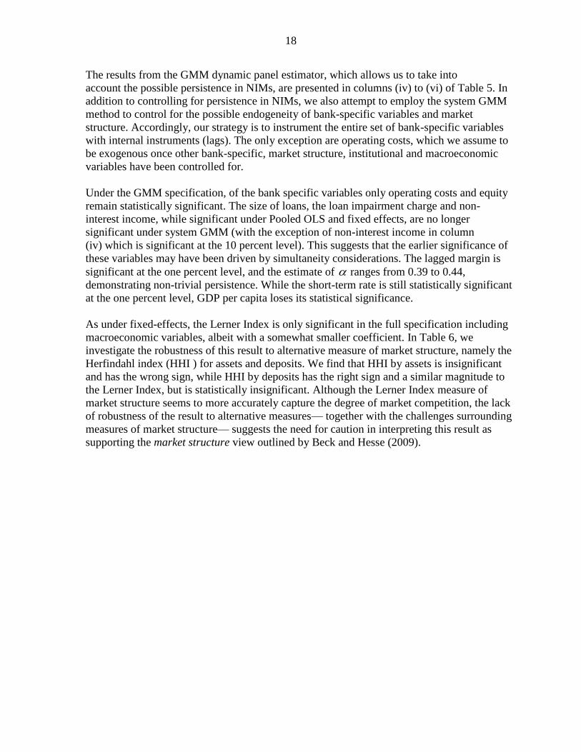
Our estimate of the impact of institutions on operating costs remains significant at the one
percent level after including additional controls. Furthermore, the size of the coefficient does
not change drastically from our original specification (column (i)). Only if we include GDP
per capita, which is highly collinear with institutions, do we find that the coefficient estimate
falls from -0.09 to -0.07. Despite the likely effect of inflating standard errors due to including
GDP per capita, which is itself insignificant, the measure of institutions remains significant at
the 10 percent level. Among our controls, only tertiary educational enrollment seems to be a
statistically significant determinant of operating costs, with a negative sign and 10 percent
significance level. The size of the loan book remains significant except in two specifications
(columns (ii) and (iii)). In contrast to Gelos (2009), we find no evidence that lack of
competition, as measured by the Lerner Index, causes banks to incur higher operating costs.
Our results suggest that better institutions reduce the need for financial intermediaries to
engage in costly monitoring and costly recovery of assets in case of default. Conversely,
countries with lower measures of institutional quality are interpreted as presenting banks with
an environment of high asymmetries of information and related costs. In this sense, we see
the results presented in Tables 4 and 5 as supporting the risk-based view of why we observe
high NIMs. Their quantitative implications are explored in more depth in the section below
(Table 9).
B. Fixed Effects and System GMM
Although our pooled OLS results provide a first pass of the potential factors driving NIMs,
the Breusch-Pagan Lagrange Multiplier test indicates that hypothesis that bank-specific
effects are present cannot be rejected (the Chi-squared test statistic is very large).
Furthermore, the Hausman test indicates that the hypothesis that bank-specific effects are
correlated with other regressors cannot be rejected in our preferred specification (iii), making
pooled OLS estimation biased for reasons explained in section III. Thus, the fixed effects
specification is the appropriate representation of the data generating process.16
The results of our fixed-effects regressions are presented in columns (i)-(iii) of Table 5. They
are similar in magnitude to those derived from pooled OLS. An examination of each column
of the table suggests that the sign and significance of each of the bank-specific variables is
preserved under fixed effects. Among macroeconomic variables, the coefficient on short-
term interest rates also appears to maintain size, sign and significance. The inclusion of fixed
effects does, however, have the effect of eliminating the significance of inflation and
exchange rate depreciation, while also making GDP per capita significant at the 10 percent
level. Finally, we observe that, the Lerner Index is statistically significant with a positive
sign, but only if we include the full set of macroeconomic controls.17
16
If the Hausman test did reject the null hypothesis, the correct specification would be random effects, which
assumes that the unobserved characteristics are uncorrelated with the regressors.
17 This result that might be accounted for by the regression in column (ii) being mis-specified. Specifically, the
presence of omitted variables will bias the estimated coefficient, while also reduce the variance of the
explanatory variables, inflating the standard errors.
18
The results from the GMM dynamic panel estimator, which allows us to take into
account the possible persistence in NIMs, are presented in columns (iv) to (vi) of Table 5. In
addition to controlling for persistence in NIMs, we also attempt to employ the system GMM
method to control for the possible endogeneity of bank-specific variables and market
structure. Accordingly, our strategy is to instrument the entire set of bank-specific variables
with internal instruments (lags). The only exception are operating costs, which we assume to
be exogenous once other bank-specific, market structure, institutional and macroeconomic
variables have been controlled for.
Under the GMM specification, of the bank specific variables only operating costs and equity
remain statistically significant. The size of loans, the loan impairment charge and non-
interest income, while significant under Pooled OLS and fixed effects, are no longer
significant under system GMM (with the exception of non-interest income in column
(iv) which is significant at the 10 percent level). This suggests that the earlier significance of
these variables may have been driven by simultaneity considerations. The lagged margin is
significant at the one percent level, and the estimate of ranges from 0.39 to 0.44,
demonstrating non-trivial persistence. While the short-term rate is still statistically significant
at the one percent level, GDP per capita loses its statistical significance.
As under fixed-effects, the Lerner Index is only significant in the full specification including
macroeconomic variables, albeit with a somewhat smaller coefficient. In Table 6, we
investigate the robustness of this result to alternative measure of market structure, namely the
Herfindahl index (HHI ) for assets and deposits. We find that HHI by assets is insignificant
and has the wrong sign, while HHI by deposits has the right sign and a similar magnitude to
the Lerner Index, but is statistically insignificant. Although the Lerner Index measure of
market structure seems to more accurately capture the degree of market competition, the lack
of robustness of the result to alternative measures— together with the challenges surrounding
measures of market structure— suggests the need for caution in interpreting this result as
supporting the market structure view outlined by Beck and Hesse (2009).

19
Table 5: Determinants Of Net Interest Margins (fixed effects and system GMM)
Net interest margin (i) (ii) (iii) (iv) (v) (vi)
Lagged net margin - - - 0.390*** 0.442*** 0.391***
[3.296] [5.439] [4.915]
Operating costs/assets (log) 1.820*** 1.701*** 1.655*** 2.323*** 1.326*** 1.582***
[5.817] [6.120] [6.005] [3.773] [3.809] [3.730]
Equity/assets (log) 1.236*** 1.245*** 1.217*** 0.626 1.431*** 0.985***
[7.299] [6.928] [7.047] [1.532] [3.742] [2.858]
Loans (log) 0.483*** 0.544*** 0.449*** 0.339 -0.209 0.145
[3.044] [3.729] [3.158] [1.120] [-1.551] [0.973]
Liquid/total assets 0.00474 0.000394 0.0000927 -0.00501 -0.00515 -0.0121
[0.908] [0.0844] [0.0187] [-0.636] [-0.528] [-1.357]
Loan impairment charge/assets (log) 0.247*** 0.263*** 0.265*** -0.0303 0.112 0.056
[5.341] [5.611] [5.676] [-0.249] [1.332] [0.740]
Non-interest activity/assets -0.329*** -0.270*** -0.274*** -0.263* -0.225 -0.221
[-4.752] [-4.403] [-4.581] [-1.674] [-1.581] [-1.468]
Lerner Index 0.502 1.174*** -0.23 0.785**
[1.510] [3.101] [-0.745] [2.083]
Inflation -0.00695 -0.00198
[-0.650] [-0.142]
T-Bill rate 0.0701*** 0.0929***
[2.765] [4.751]
USD exchange rate (% change) -0.00684 -0.00566
[-1.250] [-0.948]
GDP per capita (log) -0.000241* -0.0000188
[-1.961] [-0.481]
Constant -1.066 -1.174 -1.294 -3.069 -0.518 -2.192**
[-1.045] [-1.265] [-1.313] [-1.524] [-0.462] [-2.057]
R -squared 0.258 0.246 0.268
Observations 1524 1400 1399 1314 1208 1208
Number of banks 213 210 210 212 209 209
Hausman test p-value [0.0046] [0.1408] [0.0368]
No. of instruments 99 118 118
Hansen test p-value 0.579 0.267 0.294
A-B AR(1) test p-value 0.000976 0.0000221 0.0000833
A-B AR(2) test p-value 0.39 0.441 0.655
Fixed effects System GMM
Notes: For fixed effects, robust t-statistics in brackets. *** p<0.01, ** p<0.05, * p<0.1. For system GMM, Windmijer (2005) robust two-step
statistics reported in brackets.

20
Table 6: Role Of Alternative Measures Of Market Structure (system GMM)
Net interest margin (i) (ii) (iii)
Lagged net margin 0.391*** 0.445*** 0.434***
[4.915] [3.804] [3.795]
Operating costs/assets (log) 1.582*** 1.459*** 1.489***
[3.730] [3.174] [3.175]
Equity/assets (log) 0.985*** 0.775** 1.041***
[2.858] [2.361] [2.945]
Loans (log) 0.145 0.0637 0.0352
[0.973] [0.284] [0.168]
Liquid/total assets -0.0121 -0.00199 -0.00577
[-1.357] [-0.209] [-0.663]
Loan impairment charge/assets (log) 0.056 -0.0861 -0.0538
[0.740] [-0.847] [-0.445]
Non-interest activity/assets -0.221 -0.0783 -0.0686
[-1.468] [-0.485] [-0.425]
Inflation -0.00198 -0.0182 -0.0134
[-0.142] [-1.257] [-0.922]
T-Bill rate 0.0929*** 0.0668*** 0.0816***
[4.751] [4.135] [4.503]
USD exchange rate (% change) -0.00566 -0.00923 -0.0068
[-0.948] [-1.418] [-0.940]
GDP per capita (log) -0.0000188 -0.00000511 -6.38e-05*
[-0.481] [-0.109] [-1.702]
Lerner Index 0.785**
[2.083]
HHI (assets)-2.265
[-1.343]
HHI (deposits)0.99
[1.146]
Constant -2.192** -1.222 -2.222
[-2.057] [-0.761] [-1.451]
Observations 1208 1295 1284
Number of banks 209 210 210
No. of instruments 118 118 118
Hansen test p-value 0.294 0.354 0.163
A-B AR(1) test p-value 0.0000833 0.000635 0.000549
A-B AR(2) test p-value 0.655 0.526 0.403
System GMM
Notes: For fixed effects, robust t-statistics in brackets. *** p<0.01, ** p<0.05, * p<0.1. For
system GMM, Windmijer (2005) robust two-step statistics reported in brackets.

21
The validity of the system GMM procedure was verified through the Windmijer correction
and Hansen J test. The Windmijer (2005) correction was used in order to overcome the
downward bias that may arise from the two-step standard errors on estimated coefficients in
small samples. In addition, as documented by Anderson and Sorensen (1996) and Bowsher
(2002), a large instrument count in the system GMM weakens the power of the Hansen J-test
in testing for instrument validity. This issue is nontrivial, as in system GMM the instrument
grows quadratically in T, opening up the possibility of over fitting. To guard against this
possibility, we apply the ‗collapse‘ procedure recommended by Roodman (2009), which has
the effect of making the instrument count invariant in T. The AR-2 test and the Hansen J test,
reported at the bottom of each column, indicate that the over identifying restrictions implied
by the GMM procedure are not rejected.
Table 7: Economic Significance Of Net Interest Margin Determinants For the Whole Sample.
The economic significance of the regression results can be readily inferred from Tables 7 and
8. Table 7 shows the effect on NIMs of a one standard deviation change in one of the
explanatory variables using our baseline specification – including bank-specific, market
structure and macroeconomic variables, but excluding institutional factors (again, this
corresponds to regressions (iii) in Table 3, and regressions (iii) and (vi) in Table 6).
Parameter estimates from Pooled OLS, fixed effects and system GMM are considered. For
system GMM, the long-run effect of a change in each variable, calculated as , where 0.391 is the estimated value of the coefficient on the lagged dependent variable. Both
operating costs and equity tend to dominate the effect of other variables. A one standard
deviation increase in operating costs, amounting to a rise in the log of operating costs-to-
assets of 0.47, is associated with an increase in NIMs between 0.77 (fixed effects estimate)
and 1.21 percentage points (system GMM estimate). A one standard deviation increase in
equity, equivalent to an increase in the log of the equity/asset ratio of 0.61, is associated with
a rise in net interest margins by between 0.74 (fixed effects estimate) and 0.98 (system GMM
estimate). While the economic impact of a one standard deviation increase in the t-Bill rate
and Lerner Index are also non-trivial, they are lower than for either of the two bank-specific
variables. If interpreted causally, the effect of a one standard deviation change in T-Bill rates
of 4.06 percentage points raises net interest margins by 0.62 percentage points in the long
run, according to our system GMM estimates. A one standard-deviation increase in the
Lerner Index raises NIMs by the same amount, i.e. 0.62 percentage points.
Net interest margin POLS FE GMM Mean S.D. POLS FE GMM
Operating costs/assets (log) 2.250*** 1.655*** 1.582*** 1.56 0.47 1.05 0.77 1.21
Equity/assets (log) 1.310*** 1.217*** 0.985*** 2.42 0.61 0.80 0.74 0.98
Loans (log) 0.225*** 0.449*** 0.145 4.53 1.59 0.36 0.71 0.38
Liquid/total assets -0.00613 0.0000927 -0.0121 27.90 16.02 -0.10 0.00 -0.32
Loan impairment charge/assets (log) 0.241*** 0.265*** 0.056 -0.46 1.18 0.28 0.31 0.11
Non-interest activity/assets -0.281*** -0.274*** -0.221 3.17 2.01 -0.56 -0.55 -0.73
Lerner Index 1.230*** 1.174*** 0.785** -0.06 0.48 0.59 0.57 0.62
Inflation 0.0350** -0.00695 -0.00198 5.84 4.42 0.15 -0.03 -0.01
T-Bill rate 0.125*** 0.0701*** 0.0929*** 8.21 4.06 0.51 0.28 0.62
USD exchange rate (% change) -0.0164** -0.00684 -0.00566 -2.04 9.57 -0.16 -0.07 -0.09
log GDP per capita (USD) 0.0000281 -0.000241* -0.0000188 1811.03 2611.66 0.07 -0.63 -0.08
Coefficient estimates Effect of 1 s.d. on margins
Notes: The economic impat of net interest margins was found by multiplying the standard deviation of each explanatory variable by
the respective coefficient estimate. For system GMM, the table shows the permanent effect, calculated as beta/(1-alpha).

22
Table 8: Economic Significance Of Operating Cost Determinants (indirect impact on NIMs)
In Table 8, the economic significance of the determinants of operating costs, through their
final impact on NIMs is considered. A one standard deviation in the log of the size of the
loan book reduces NIMs, through lowering operating costs, by 0.25 percentage points. A one
standard deviation improvement in our synthetic indicator of institutions, roughly equivalent
to the difference between Burundi and South Africa in 2011, for instance, has an even greater
impact, with NIMs predicted to fall by 0.33 percentage points.
Table 9: Regional Comparison Using 2011 Values and System GMM Estimates
The results in Table 9 reinforce earlier conclusions (Table 8) from a regional perspective, by
calculating the contribution to the average NIMs in each region implied by our system GMM
regression estimates, using values for 201118. We observe that, together, operating costs and
equity/assets explain the vast proportion of the predicted NIMs in every region. For instance,
in the EAC, operating costs account for 2.4 percentage points, equity/assets 1.9 percentage
18
The average NIM and value of explanatory variable is computed as an arithmetic average of the bank
variables.
Operating costs (log) POLS Mean S.D.
Loans (log) -0.0609*** 4.53 1.59 -0.25
Non-performing Loans (log) 0.0142 1.67 1.38 0.05
Lerner Index 0.0199 -0.06 0.48 -0.02
WGI Composite -0.0917*** -0.93 1.38 -0.33
Indirect impact on margins
Notes: The effect of each variable on operating costs was calculated using the POLS result in Table 4,
column (vii). Subsequently, the indirect impact on net interest margins was calculated using the GMM
results in column (vi) in Table 6. The table shows the permanent effect, calculated as beta/(1-alpha).
Net interest margin EAC CEMAC ECCU WAEMU SACU
Operating costs/assets (log) 2.37 1.45 1.31 2.08 1.84
Equity/assets (log) 1.90 1.33 1.64 1.47 2.17
T-Bill rate 1.48 0.61 0.90 0.65 0.97
Lerner Index 0.15 0.19 -0.27 0.18 -0.14
Implied net interest margin 5.75 3.39 3.84 4.20 4.98
True net interest margin 6.19 4.16 2.84 3.67 4.93
Error 0.44 0.64 -1.17 -0.70 -0.24
Notes: The 'contribution' of each explanatory variable for the region was calculated as follows. Firstly, we obtained the values of
each bank-specific explanatory variable for a region as an arithmetic average of all the banks in that region. Secondly, this value
was multiplied by the system GMM coefficient estimate for that variable. The table shows the permanent effect, calculated as
beta/(1-alpha).

23
points and short-term interest rates 1.5 percentage points respectively of NIMs, yielding an
implied net interest margin at 5.8, in comparison to the actual margin in 2011 of 6.2.
VI. CONCLUDING REMARKS
The main finding of our study is that operating costs and equity-to-capital ratios are both
statistically and economically significant determinants of NIMs in the SSA and the Eastern
Caribbean. Additionally, operating costs are strongly and inversely related to the size of bank
loan portfolios, suggesting that fixed costs to lending are significant, and that there is scope
for large banks to exploit economies of scale. We also find evidence for a statistically
significant, but quantitatively less strong, role of treasury bill rates on NIMs. The importance
of the treasury bill rate supports the idea that banks respond to an increase in the cost of
capital by increasing the spread between borrowing and lending rates, consistently with the
predictions of Bernanke, Gertler and Gilchrist (1999) and Kiyotaki and Moore (1997).
The results suggest considerable evidence for the risk-based and small-financial system
views. This is based on the significance of operating costs, specifically in the role of
institutions and economies of scale. In addition, there is some evidence for the role of the
macroeconomic hypothesis, based on the significance of the short-term interest rate, and
some evidence for the market-structure view reflecting the significance of the Lerner index.
Nonetheless, the lower economic significance of these variables in explaining NIMs suggests
that the macroeconomic and market-structure hypotheses are less important in the regions
under study.
A further contribution of this paper is the finding that institutional factors may indirectly
contribute to higher operating costs. This underscores the impact of gaps in regulatory quality
and the application of the rule of law on higher costs of credit appraisal, monitoring and asset
recovery. The results are therefore consistent with anecdotal evidence that the poor
institutional climate could result in banks engaging in costly monitoring or screening
activities which, in turn, leads to higher margins.
24
REFERENCES
Abiad, A., N. Oomes and K. Ueda (2008), ―The quality effect: Does financial liberalization
improve the allocation of capital?‖, Journal of Development Economics 87 270-282.
Ahokpossi, C. (2012), ―Determinants of bank interest margins in sub-Saharan Africa‖,
Mimeo., IMF, Washington, DC.
Anderson, T. G. and B. E. Sørenson (1996), ―GMM estimation of a stochastic volatility
model: A Monte Carlo study‖, Journal of Business and Economic Statistics 328–352.
Angrist, J. D. and J. Pischke (2008), Mostly Harmless Econometrics: An Empiricist’s
Companion, Princeton University Press, Princeton, NJ, USA.
Arellano, M., and S. R. Bond (1991), ―Some tests of specification for panel data: Monte Carlo
evidence and an application to employment equations,‖ Review of Economic Studies 58 277–
97.
Arellano, M. and O. Bover (1995), ―Another look at the instrumental variable estimation of error-
components models‖, Journal of Econometrics 68 29–51.
Baltagi, B. H. (2008), Econometric Analysis of Panel Data, 4th
ed., John Wiley & Sons.
Banerjee, A. B. and E. Duflo (2005), ―Do firms want to borrow more? Testing credit
constraints using a directed lending program‖, Mimeo., MIT.
Banerjee, A. B. and E. Duflo (2010), ―Giving credit where it is due‖, CEPR Discussion Paper
No. 7754.
Barth, J., G. Caprio and R. Levine (2003), ―Bank regulation and supervision: What works
best?‖ Journal of Financial Intermediation 13 205–48.
Beck, T. and H. Hesse (2009), ―Why are interest spreads so high in Uganda?‖, Journal of
Development Economics, 88 192-204.
Bernanke, B. S., M. Gertler and S. Gilchrist (1999), ―The financial accelerator in a
quantitative business cycle framework‖, ed. J. B. Taylor and M. Woodford, Handbook of
Macroeconomics, Volume 1, 1341-1393.
Blundell, R. and S. Bond (1998), ―Initial conditions and moment restrictions in dynamic
panel data models‖, Journal of Econometrics 87 115-143.
Bolton P. and X. Freixas (2007), ―Corporate finance and the monetary transmission
mechanism‖, Review of Financial Studies 19 829-870.
Bottomley, A. (1963), ―The Cost of Administering Private Loans in Underdeveloped Rural
Areas,‖ Oxford Economic Papers 15 154-163.

25
Bowsher, C. G. (2002), ―On testing overidentifying restrictions in dynamic panel data
models‖, Economics Letters 77 211-220.
Chami, R. and T. F. Cosimano (2010), ―Monetary policy with a touch of Basel‖, Journal of
Economics and Business 62 161-175.
Claessens, S. and L. Laeven (2004), ―What drives bank competition? Some international
evidence‖, Journal of Money, Credit and Banking 36 563-583.
Deaton, A. (1995), ―Data and econometric tools for development analysis‖, Ch. 33, eds.
Behrman, J. and T. N. Srinivasan, Handbook of Development Economics, Volume III,
Elsevier Science B.V.
Demirguc-Kunt, A., L. Laeven and R. Levine (2004), ―Regulations, market structure,
institutions, and the cost of financial intermediation‖, Journal of Money, Credit, and
Banking 36 593-622.
Djankov, S., O. Hart, C. McLiesh and A. Shleifer (2006), ―Debt enforcement around the
world‖, NBER Working Paper 12807.
Djankov, S., C. McLiesh and A. Shleifer (2007), ―Private credit in 129 countries‖, Journal of
Financial Economics 84 299-329.
Galindo, A., F. Schiantarelli and A. Weiss (2007), ―Does financial liberalization improve the
allocation of investment? Micro-evidence from developing countries‖, Journal of
Development Economics 83 562-587.
Gelos, G. (2009), ―Banking spreads in Latin America‖, Economic Enquiry 47 796-814.
Ho, T and A. Saunders (1981), ―The determinants of bank interest margins: theory and
empirical evidence‖, Journal of Financial Quantitative Analysis 16 581-600.
Holmstrom, B. and J. Tirole (1997), ―Financial intermediation, loanable funds, and the real
sector‖, Quarterly Journal of Economics 112 663-691.
Honohan, P. ―The Accidental Tax: Inflation and the Financial Sector.‖ In Taxation of
Financial Intermediation, Theory and Practice for Emerging Economies, edited by P.
Honohan . Washington DC: World Bank Publications and Oxford University Press, 2003
381–420
Honohan, P. and T. Beck (2007), ―Making finance work for Africa‖, World Bank,
Washington, DC, USA.
Kaufman, D. A. Kraay and G. Mastruzzi (2005), ―Governance matters IV: governance
indicators 1996-2005‖, World Bank Policy Research Working Paper 3630.
Karlan, D. and J. Zinman (2009), ―Observing Unobservables: Identifying Information
Asymmetries with a Consumer Credit Field Experiment‖, Econometrica 77 1993-2008.

26
Kiyotaki, N. and J. Moore (1997), ―Credit cycles‖, Journal of Political Economy 105 211-
248.
Levine, R., N. Loayza and T. Beck (2000), ―Financial intermediation and growth: Causality
and causes‖, Journal of Monetary Economics 46 31-77.
Martinez Peria, S., and A. Moody (2004), ― How Foreign Participation and Market
Concentration Impact Bank Spreads: Evidence from Latin America‖ Journal of Money
Credit and Banking, 36, 511-537.
Maudos, J., and J. Fernandez de Guevara (2004), ―Factors explaining the interest margin in
the banking sectors of the European Union‖, Journal of Banking and Finance 28, 2259-
2281.
Nickell, S. (1981), ―Biases in dynamic models with fixed effects‖, Econometrica 49, 1417-
1426.
Petersen, M. A and R. G. Rajan (1995), ―The effect of credit market competition on lending
relationships‖, Quarterly Journal of Economics 110 407-443.
Poghosyan, T. (2010), ―Re-examining the impact of foreign bank participation on interest
margins in emerging markets‖, Emerging Markets Review 11 390-403.
Poghosyan, T. (2012), ―Financial Intermediation Costs in Low-Income Countries: The Role
of Regulatory, Institutional, and Macroeconomic Factors‖, IMF Working Paper
WP/12/140, IMF, Washington, DC.
Randall, R (1998), ―Interest rate spreads in the Eastern Caribbean‖, IMF Working Paper
WP/98/59, IMF, Washington, DC.
Rajan, R. G. and L. Zingales (1998), ‗Financial Dependence and Growth‘, American
Economic Review 88 559-586.
Rosse, J. N. and J. C. Panzar (1977), ―Chamberlin versus Robinson: An empirical test for
monopoly rents‖, Studies in Industry Economics, Research Paper no. 77, Stanford
University, Stanford, California.
Stiglitz, J. E. and A. Weiss (1981), ―Credit Rationing in Markets with Imperfect
Information‖, American Economic Review 71 393-410.
Wakeman-Linn, J. A. Jarotschkin, A. Bashagi, P. Kessy and W. Reweta (2010), ―Bank
Spreads in the EAC: 1998-2010‖, mimeo.
VanHoose, D. D. (2008), ―Bank capital regulation, economic stability, and monetary policy:
what does the academic literature tell us?‖, Atlantic Economic Journal 36 1-14.

27
Appendix I
Measuring Market Competition
We examine three different measures of competition in the banking sector as a check for
robustness: the Herfindahl-Hirschman Index (HHI) by assets, the HHI by deposits and the
Lerner Index. This section clarifies our computation of these measures. The Lerner Index ictli
for bank i is a direct measure of pricing behavior by banks, and captures the markup in
prices. It is defined as the difference between prices ictp and marginal costs ictmc , measured
as a ratio of prices:
ict
ict ict
ict
p mcli
p
The Lerner Index for a market is a weighted sum of Lerner Indices for particular banks,
and is defined as
ct ict ict
i c
li w li
where i indexes banks, c indexes countries, t indexes time and ictw is the weight of bank i in
country c in year t. The weight represents the fraction of the total assets in country c of the
assets of bank i in year t. The marginal cost component of the index is calculated by taking
the derivative with respect to assets of the following translog regression for total costs
2
1 1 2
3 3 3
1 1 1
1ln ln (ln )
2
1 1ln ln ln ln
2 2
ln ln
it it it
jk jkt kit jk it jit
j k j
ict ict it
c q q
w w q w
equity lend u
(0.1)
where itc denote total bank costs, itq denote total bank assets. 3
1{ }it iw denote, respectively,
the ratio of personnel costs over total assets, the ratio of non-personnel operating costs over
total assets, and interest expenses over total funding, ictequity is the ratio of equity to total
assets, while ictlend denotes the ratio of net total lending to total assets. The price component
ictp is calculated as the ratio of total bank income to total bank assets.
Our other measure of market structure, the HHI, is perhaps the most widely used
measure of competition. It is based on market shares, and is defined as
2
ct ict
i c
HHI s
(0.2)
where icts is the market share of firm i in country c, where market share is either of deposits
or of assets, depending on the measure of concentration used.

28
Appendix II