Banking Efficiency and Financial Development in Sub-Saharan Africa

Sandrine Kablan

WP/10/136

© 2010 International Monetary Fund WP/10/136 IMF Working Paper African Department

Banking Efficiency and Financial Development in Sub-Saharan Africa

Prepared by Sandrine Kablan1

Authorized for distribution by Tsidi Tsikata

June 2010

Abstract

This Working Paper should not be reported as representing the views of the IMF. The views expressed in this Working Paper are those of the author(s) and do not necessarily represent those of the IMF or IMF policy. Working Papers describe research in progress by the author(s) and are published to elicit comments and to further debate.

This study assesses the determinants of banking system efficiency in sub-Saharan Africa (SSA) and asks what, besides the degree of efficiency, explains the low level of financial development in the region. It uses stochastic frontier analysis to measure efficiency and a generalized method of moments system to explain financial development. SSA banks are found to be generally cost-efficient, but nonperforming loans undermine efficiency, which suggests that improvement in the regulatory and credit environments should improve efficiency. The political and the economic environment have held back financial development in SSA. JEL Classification Numbers: G21, O16, O55 Keywords: Cost-efficiency, Stochastic Frontier Analysis, Banking System, Financial

Development, Sub-Saharan Africa Author’s E-Mail Address:

sandrinekablan@hotmail.com

1 Work on this paper started during the author’s summer internship at the African Department of the IMF in 2007. She wishes to thank Mr. Shanaka Peiris for his guidance, Messrs. Johannes Mueller and Tsidi Tsikata, other colleagues in the Department for their comments, and Ms. Anne Grant for editorial assistance. Any remaining errors are the author’s responsibility.

2

Contents Page

I. Introduction ............................................................................................................................3 

II. Literature Review ..................................................................................................................4 A. Bank Efficiency .........................................................................................................4 B. Financial Development .............................................................................................6 

III. Banking Efficiency in Sub-Saharan Africa ........................................................................10 A. Methodology ...........................................................................................................10 B. Data and Results ......................................................................................................13 

IV. Financial Development in Sub-Saharan Africa .................................................................16 A. Methodology ...........................................................................................................16 B. Data and Results ......................................................................................................18 

V. Conclusion ..........................................................................................................................18 

References ................................................................................................................................21  Tables 1. Average Logarithmic Values Used for the Arguments of the Cost Frontier Function ........14 2. Results of the Translogarithmic Cost-frontier Function Using the One-Step Method ........15 3. Average Cost-efficiency Score Measured by the Translogarithmic Cost Function ............16 4. GMM Estimation for Financial Development Determinants...............................................19  Figures 1. Evolution of the M2/GDP Ratio for Sub-Saharan Africa, Latin America, and Asia, 1980–2002...............................................................................................................................7 2. Evolution of the M2/GDP Ratio by SSA Regions, 1980–2002 .............................................8 3. Evolution of Credit to the Private Sector in Sub-Saharan Africa, Latin America, and Asia, 1980–2002 .....................................................................................................................9 4. Evolution of Credit to the Private Sector in Sub-Saharan Africa, 1980–2002 ......................9  Appendix I. GMM Regression Including the Cost Efficiency Scores Derived from the Stochastic Frontier Function .................................................................................................25 

3

I. INTRODUCTION

Financial development is crucial to economic growth.2 In sub-Saharan Africa (SSA), banks are the most important element of the financial system. In many countries, other financial structures are underdeveloped or almost nonexistent. There have been several studies of banking crises in SSA (Honohan, 1993; Powo, 2000; Daumont, Le Gall and Le Roux, 2004). The 1990s were a period of financial reforms in developing countries. Studies have been done on banking efficiency and competitiveness to assess the impact of those reforms, usually on groups of emerging countries (Grigorian and Manole, 2002; Bonin, Hasan and Wachtel, 2005; Boubakri, Cosset, Fischer and Guedahmi, 2005; Fries and Taci, 2005) but sometimes on a single country (Hauner and Peiris, 2005; Buchs and Mathiesen, 2005). Banks have three principal activities: taking deposits, making loans, and investing in securities. To do this they use labor (skilled and unskilled), physical capital, and financial capital. Two main questions are addressed in this study: (i) How efficient are banks in SSA and what determines their degree of efficiency? (ii)What other factors may explain the low level of financial development in SSA? To answer these questions, the paper uses stochastic frontier analysis to assess banking efficiency and its determinants. This method makes it possible to determine the cost frontier while taking into account factors related to both the technological process of banks and the environment in which they operate. To investigate the low level of financial development, the paper employs the generalized method of moments (GMM) system of Arellano and Bover (1995). The results show that on average, SSA banks are cost-efficient in producing their main outputs—deposits and short-term loans. However, efficiency could be improved by enhancing the credit environment through better functioning judicial and legal processes and the accessibility of information on borrowers. This should allow banks more effectively to play their financial intermediary role of transforming deposits into loans for investment. The estimations show that financial development has been hindered by inflation and somewhat by concentration in the banking sector. Better macroeconomic stabilization policies that keep inflation under control and a more competitive banking system could help financial development. In what follows, Section II reviews the literature on the efficiency of banks and on financial development in SSA and other developing areas. Section III presents the methodology and results of the assessment of banking efficiency in SSA. Section IV discusses the degree of financial development in SSA. Conclusions are presented in Section V.

2 See, for example, Levine (1997) and Greenwood and Javanovic (1990).

4

II. LITERATURE REVIEW

A. Bank Efficiency

Efficiency is related to the ability to produce a result with minimum effort or resources. It measures how close a production unit gets to its production possibility frontier, which is composed of sets of points that optimally combine inputs in order to produce one unit of output. Following Harker and Zenios (2000), the drivers of bank performance are grouped into three broad categories: strategy, execution of strategy, and environment. Strategy

The articulation of a strategy is a key driver for success in dynamic, competitive environments like that of the financial services industry. The main strategic choices a bank faces concern product mix, client mix, geographical location, distribution channels, and form of organization. Choosing a product mix not only defines the strategy of the institution in providing services but is also a strategic decision in risk management—it is in effect the choice of financial risks the institution plans to manage. SSA banks have adopted a strategy that gives deposits a large share in the outputs combination they offer. The intermediation ratio (claims on the private sector relative to total deposits) of SSA banks is smaller than in other developing countries, suggesting that African banks have difficulty transforming collected deposits into loans to the private sector. For example, in 2003 SSA as a whole displayed an intermediation ratio of 57 percent, compared to 91 percent for Asia and 75 percent for Latin America.3 A successful strategic decision regarding client mix hinges upon matching a targeted client segment with well-priced products. Besides orienting their activities toward collecting deposits, banks in SSA make loans to clients with good capacity for repayment. These are usually big foreign companies or domestic public ones. Local small and medium enterprises are often not considered. After the two choices of product and client mix, regulatory restrictions may determine the geographical scope of the institution. The choice of location again implies strategic choices related to risk management in bank operations. SSA banks tend to locate their branches in more economically developed regions at the expense of rural ones. There are more businesses in areas like towns, so banks can find economic activities to finance for a profit.

3 Some differences in these ratios appear among African regions: non-WAEMU west African countries have a ratio of 61 percent against 70 percent for WAEMU countries, 65 percent for Central Africa, 59 percent for Southern Africa including South Africa, and 39 percent for East Africa.

5

Execution of strategy

A strategy can be implemented through human resource management, use of technology, and process design. X-efficiency is a measure of how well management aligns technology, human resource management, and other resources to produce a given level of output. It views banks as a factory that consumes various resources to produce several products and establishes the efficiency with which this transformation takes place. The X-efficiency of banks can be assessed through indicators of financial soundness. Changes in those indicators are noticeable for SSA since the banking reforms of the 1990s. For instance, total problem loans as percent of assets decreased by 0.9 percent after the restructuring; they equaled 8.3 percent in 2003. SSA banks increased their capital as share of assets to 18.9 percent the same year against 14.5 percent during the 1990s. They also became more liquid, with the ratio of liquid assets to total assets reaching 28.8 percent.4 The effort the authorities made to align the regulatory framework with international standards like the Basel principles seem to have produced improvements. Banks are using information technology more and more in delivering transactions. As elsewhere in the world, SSA banking systems have seen many technological changes. Most of them—for example, computerization of bank processes and using Automated Teller Machines (ATMs)—were introduced by foreign banks, who imported them from their headquarters. Anglophone countries like Kenya, Nigeria, and South Africa seem to have more ATMs than Francophone countries. The creation of mobile banking units in Kenya and the use of chip/fingerprint technology in Malawi to increase access to financial services are other examples of technology adoption. The differences between Francophone and Anglophone countries could be due to the degree of development of their financial sectors; they seem to be deeper in Anglophone countries with more banks and more branches. Environment

The environmental factors that explain efficiency are information technology, client tastes, and regulation. Banks try to influence environmental factors through lobbying activities, marketing efforts, research and development. Although Africa was not protected from technological changes, technological progress has been slow to spread because of factors that limit access, such as illiteracy and high costs. As an example, many banks in SSA offer services through the Internet, but the Internet is not widely used because of its cost but also because people are not used to this means of communication. Also the relative cost for people to access ATMs in Africa is high—because they are not widely used, the cost to banks may also be high.

4 Gulde, Patillo, and Christensen (2007).

6

After the banking crisis of the 1980s, monetary authorities in SSA tightened the regulation of banks. In each of the two Communauté Financière Africaine (CFA) subzones, a single supervisory institution was formed (Commission Bancaire de l’UMOA, for WAEMU countries and Commission Bancaire de la CEMAC, for Central Africa). Non-CFA countries gradually shifted powers of regulation and supervision solely to central banks; previously they had been shared between central banks and government ministries. By the late 1990s most countries had strengthened banking supervision. Prudential regulations were aligned with the Basel core principles and monitoring and inspections were instituted, although implementation is still weak. Hauner and Peiris (2005) investigated whether the banking sector reforms undertaken in Uganda to improve competition and efficiency have been effective. Using the model of Panzar and Rosse (1987) to assess competitiveness and data envelopment analysis (DEA) to assess efficiency, they found that competition has increased significantly and has been associated with a rise in efficiency. Using the same model, Buchs and Mathiesen (2005), found that bank size is a determining factor of bank revenue in Ghana, and foreign banks are more efficient in generating revenue (interest, commissions, and fees). Cihak and Podpiera (2005), studying East African banking reforms, found that the banking systems of Kenya, Tanzania, and Uganda were inefficient and had only a limited intermediation role, despite recent reforms and even with international banks present. Other studies pinpoint the impact of foreign bank entry into developing countries. In SSA, foreign banks hold a large share of banking system assets. They bring expertise and help enhance banking system efficiency. Kirkpatrick, Murinde and Tefula (2008) found in their study of Anglophone SSA countries that the degree of foreign bank penetration is inversely related to X-inefficiency, suggesting that foreign bank ownership in Africa has contributed to better management and performance of commercial banks. Similarly, in a study of 11 transition economies, Bonin, Hasan and Wachtel (2005) provide evidence that foreign–owned banks collect more deposits and make more loans than domestic private banks, and are more efficient in the distribution of financial services in those countries. Boubakri, Cosset, Fischer and Guedhami (2005), examining the post-privatization performance of 81 banks in 22 developing countries, found that foreign bank entry is highly beneficial, because they have more cautious risk-taking strategies.

B. Financial Development

A developed and well-functioning financial sector facilitates the exchange of goods and services, mobilizes savings, allocates resources, and helps diversify risks. At independence, SSA countries had embryonic financial systems made up of subsidiaries of foreign banks that were geared toward financing foreign trade and a very limited number of local activities. After independence, both state-owned and local private banks were created to fill gaps left by foreign banks. In many countries, selective credit policies fostered the financing of priority

7

sectors of the economy that were supposed to spur economic growth. These measures led to misallocation of resources and credit rationing and, combined with inadequate banking supervision, led to nonperforming loans (NPLs) and undercapitalized banks. In the mid-1980s economic deterioration contributed to bank failures in many SSA countries. Subsequently, reforms were implemented in many of these countries as part of structural adjustment programs supported by international financial institutions. Interest rates were liberalized, credit controls removed, and indirect monetary policy instruments introduced. The early results were mixed, and a new round of reforms was implemented in the mid-1990s. The reforms did not increase the monetization of SSA economies. Figure 1 presents the evolution of the M2/GDP ratios for SSA, Latin America, and Asia. The SSA ratio was flat at about 25 percent in 1980–2002, while in Latin America it increased from 32 percent to 52 percent and in Asia from 30 percent to 64 percent. Figure 2 shows the large differences in the level and evolution of the M2/GDP ratio within SSA.

Figure 1. Evolution of the M2/GDP Ratio for Sub-Saharan Africa, Latin America, and

Asia, 1980–2002

0

0,1

0,2

0,3

0,4

0,5

0,6

0,7

1980 1982 1984 1986 1988 1990 1992 1994 1996 1998 2000 2002

SSA

Asia

Latin America

8

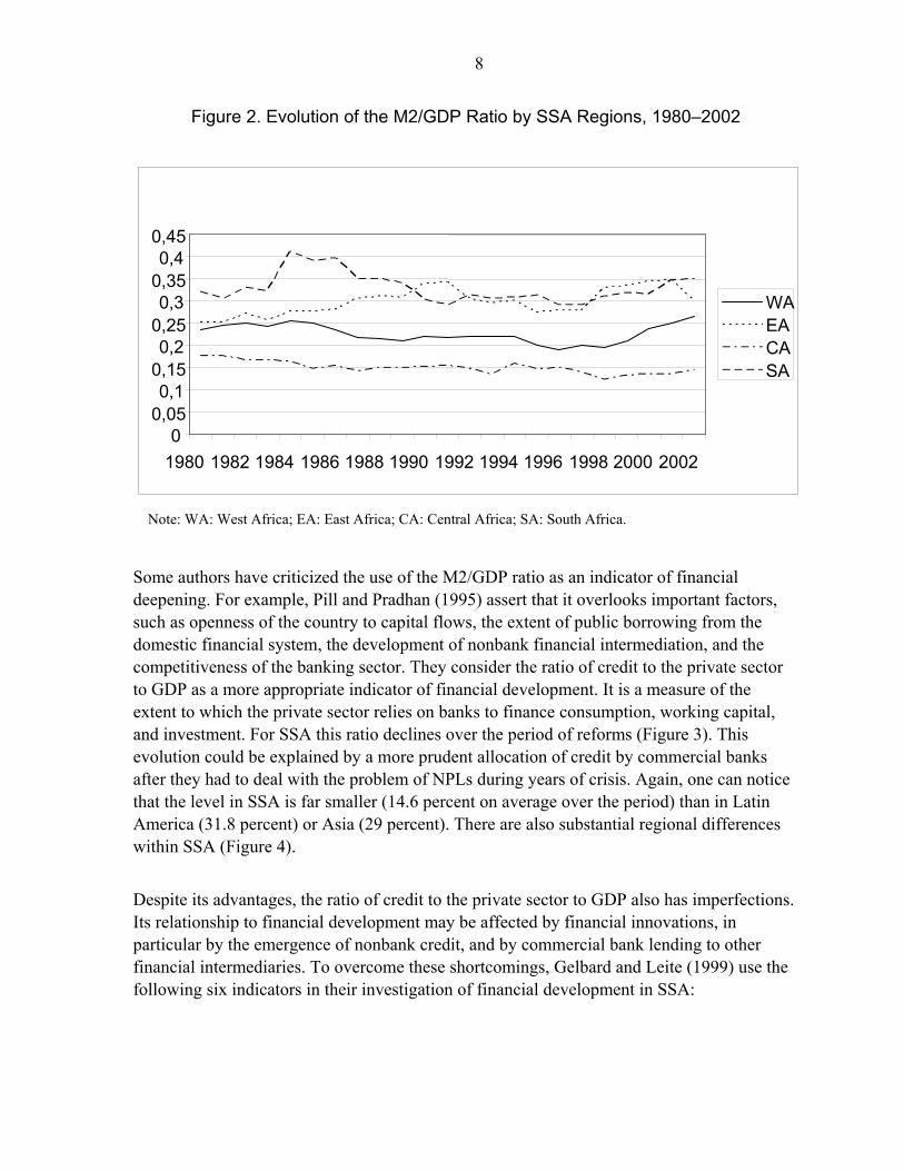
Figure 2. Evolution of the M2/GDP Ratio by SSA Regions, 1980–2002

Note: WA: West Africa; EA: East Africa; CA: Central Africa; SA: South Africa.

Some authors have criticized the use of the M2/GDP ratio as an indicator of financial deepening. For example, Pill and Pradhan (1995) assert that it overlooks important factors, such as openness of the country to capital flows, the extent of public borrowing from the domestic financial system, the development of nonbank financial intermediation, and the competitiveness of the banking sector. They consider the ratio of credit to the private sector to GDP as a more appropriate indicator of financial development. It is a measure of the extent to which the private sector relies on banks to finance consumption, working capital, and investment. For SSA this ratio declines over the period of reforms (Figure 3). This evolution could be explained by a more prudent allocation of credit by commercial banks after they had to deal with the problem of NPLs during years of crisis. Again, one can notice that the level in SSA is far smaller (14.6 percent on average over the period) than in Latin America (31.8 percent) or Asia (29 percent). There are also substantial regional differences within SSA (Figure 4).

Despite its advantages, the ratio of credit to the private sector to GDP also has imperfections. Its relationship to financial development may be affected by financial innovations, in particular by the emergence of nonbank credit, and by commercial bank lending to other financial intermediaries. To overcome these shortcomings, Gelbard and Leite (1999) use the following six indicators in their investigation of financial development in SSA:

00,05 0,1

0,15 0,2

0,25 0,3

0,35 0,4

0,45

1980 1982 1984 1986 1988 1990 1992 1994 1996 1998 2000 2002

WAEACASA

9

Figure 3. Evolution of Credit to the Private Sector in Sub-Saharan Africa, Latin

America, and Asia, 1980–2002

Figure 4. Evolution of Credit to the Private Sector in Sub-Saharan Africa, 1980–2002

Note: WA: West Afric;, EA: East Afric;, CA: Central Afric;, SA: South Africa.

00,05

0,10,15

0,20,25

0,30,35

0,40,45

0,5

1980 1982 1984 1986 1988 1990 1992 1994 1996 1998 2000 2002

SSA

Latin America Asia

0

0,05

0,1

0,15

0,2

0,25

1980 1982 1984 1986 1988 1990 1992 1994 1996 1998 2000 2002

WA

EA

CA

SA

10

market structure and competitiveness of the system; availability of financial products; degree of financial liberalization; institutional environment under which the system operates; degree of integration with foreign financial markets (financial openness); and degree of sophistication of the instruments of monetary policy.

The Gelbard and Leite survey (1999) found that some progress in financial development was noticeable in SSA but much remained to be done. Most studies of financial development investigate its impact on economic growth, and vice versa: Gurley and Shaw (1955); King and Levine (1993); Berthelemy and Varoudakis (1996); Greenwood and Smith (1997). However, others like Detragiache, Gupta, and Tressel (2005) study its determinants. They found that corruption, inflation, and foreign bank penetration have a negative impact on financial development. By contrast, better contract enforcement and information about borrowers are associated with more private sector credit.

III. BANKING EFFICIENCY IN SUB-SAHARAN AFRICA

A. Methodology

Stochastic frontier analysis

This study uses stochastic frontier analysis (SFA) to measure cost efficiency in SSA rather than DEA.5 SFA has two principal advantages: (i) it separates random error from production unit inefficiency and takes into account the existence of exogenous shocks;6 and (ii) it is less sensitive to outliers. SFA is implemented by making an econometric estimate of the best practice frontier. A production unit efficiency score is given by the ratio of the observed output to the maximum of feasible output, where the maximum is the frontier of best practice. SFA leads to estimation of the objective frontier function (cost or production function), by its specification in a Cobb-Douglas, CES, or translogarithmic function. To determine the outputs and inputs of sub-Sahara African banks, this study follows the intermediation approach and the value-added principle. According to the former, banks are supposed simultaneously to offer liquid deposits without risk and to make loans, which are

5 The DEA method is nonparametric. It offers an analysis based on relative evaluation of the efficiency in an input/output multiple situation by taking into account each bank and measuring its relative efficiency to an envelopment surface made up with the best banks. However, this method does not allow for noise treatment and does not envelop data as an econometric approach does.

6 The error term is divided into two components: an inefficiency component and a random one composed of measurement error and exogenous shocks.

11

risky assets and less liquid. 7 The latter stipulates that the elements that contribute to generate added value are regarded as outputs. Therefore, the chosen outputs are deposits, loans and securities; the inputs are labor, physical capital, and financial capital. A model adapted to the multifarious character of bank efficiency is chosen, given the multiplicity of bank functions. The translogarithmic function seems to be best adapted compared to other functional forms because it takes into account the numerous complementarities between explanatory factors, and it does not impose any restriction on the functional form. Moreover, panel data is used. Indeed, observing banks at several points in time allows for possibly better estimates. For instance, certain assumptions relating to the stochastic frontier analysis can be relaxed, allowing for more flexibility in the handling of the model. The study uses the model with random errors, in which statistical noises vary through the banks and over time, just as inefficiency does (Battese and Coelli, 1992). It applies to this model the method of maximum likelihood for the estimate of the parameters, with the current assumption of a normal truncated distribution for the inefficiency term. It also assumes that banking technology is the same in all African countries. Battese and Coelli (1995) conceived a one-step procedure for estimating the parameters of the cost function that allows for the computation of bank efficiency while taking into account its explanatory variables. This approach makes it possible to integrate into the cost frontier the impact of variables that influence cost-efficiency. These variables are taken into account in its calculation, so there is no measurement bias as in the two-steps method. 8 The computed model will be as follows:

Ln CT= α0+∑iαi lnpi +∑j ßjlnyj +1/2∑i∑kαik lnpi lnpk +1/2∑h∑jßhj lnyh lnyj +∑i∑j δij lnpi lnyj

+ zit + vit-uit (1)

with: pi : the inputs price vector yj : the ouputs value vector zit : the vector of variables that explain efficiency vit: statistical noise with the independent normal distribution N(0, σv

2) uit: the positive inefficiency term, assumed to be distributed independently of vit. The likelihood function is written as follows: 7 By contrast, with the production approach, banks are supposed to produce transaction and information services. Therefore, banking product is made up of accounts opened by the bank for managing deposits and loans.

8 The two-steps method leads to a bias because the efficiency scores are first computed without integrating factors linked to bank technological process that impact them. In the second step, the computed efficiency scores are related to explanatory variables that are likely to influence the production process and therefore the estimation of efficiency.

12

Ln L = N/2 ln(2/π)- Nlnσ – 1/2σ2Σ εi

2 + Σln [φ(εiλ/σ)] . (2) Cost-efficiency scores are calculated using the following equation: E(ui/ε) = [σλ/(1+λ2)] [φ(εiλ/σ)/ ψ (εiλ/σ) + εiλ/σ] (3) where: εi = vi-ui

σ = (σu2 + σv

2)

λ = σu/σv

φ is the standard normal density function.

ψ is the standard normal cumulative distribution.

Determinants of efficiency

As noted, some variables related to banking technology are integrated into the cost efficiency frontier. To explain efficiency many authors, such as Allen and Rai (1996), use capitalization measured by the book value of stockholder equity as a fraction of total assets and bank size, which is the ratio of one bank’s deposits to all banking system deposits. The theory is that bank capitalization could have a significant impact on efficiency. Besides, larger banks take advantage of scale economies through shared costs in the production process. Another important consideration is bank ownership. Studies of the banking system of developing countries or transition countries always stress the importance of ownership. Foreign-owned banks tend to import good methods and the expertise of parent companies into the environment where they operate. They also have more financial resources to face specific problems. Other variables related to the environment affect bank cost-efficiency. GDP per capita (GDPc) is one explanatory variable because it affects numerous factors related to demand for and supply of banking services. Countries with higher per capita income have banking systems that operate in a more mature environment, resulting in more competitive interest rates and profit margins. Therefore, GDP per capita is expected to have a negative impact on bank cost and a positive impact on cost efficiency. Other variables identified in the literature as having a specific impact on developing country bank efficiency are also considered. NPLs, as indicated above, are a key variable used to assess the soundness of the banking system (how well the system is improving its risk management). Bad loans tend to increase bank production costs, reflecting inefficiency in lending. Kirkpatrick, Murinde and Tefula (2008) argue that inefficiency mainly arises from

13

bad loans. The variable is defined as the ratio of NPLs to total loans in each country.9 It captures the negative impact of problem loans that SSA banks face. Another variable that can have a specific impact on bank efficiency is the percentage of the population living in rural areas. Banks in developing countries, especially in Africa, tend to be located in towns because most of their customers are city dwellers. Banks in countries with a high share of rural population tend to be less cost-efficient because they cannot realize economies of scale. A positive sign is expected for the coefficient.

B. Data and Results

The sample for the cost efficiency estimate is made up of 137 banks in 29 African countries. Generally the sample was constructed as follow: on average five banks were chosen in each African country. For countries like Ghana, Kenya, Nigeria, and South Africa with numerous banks, the number selected was proportionally increased. Among these banks, some are not observed over the entire period considered. Bankscope was the source for the arguments of the stochastic cost-frontier estimation. Variables integrated in the cost frontier function and used to explain it come from International Financial Statistics (ratio of private loans to GDP), World Development Indicators (GDP per capita, share of rural population), and the country profile data set of the IMF African Department (NPLs). Variables like capitalization and bank size are calculated using Bankscope and International Financial Statistics (IFS). To determine bank ownership, information from country economists of the IMF African Department was used to build a dummy variable named Foreign_dummy (equal to one when the bank is a foreign one and 0 otherwise). The average logarithmic values of the variables used as arguments of the cost frontier function are presented in Table 1. Table 2 shows the estimate of the cost-efficiency frontier with the software Frontier 4.1 of Battese, Coelli and Rao (1998). The gamma coefficient (γ = σu

2/(σu2 + σv

2)), is significant indicating the existence of the cost frontier function. This result enables us to reject the assumption according to which the variance of the inefficiency term σu

2 is null.10 Consequently, the uit term cannot be isolated from the regression, and the cost frontier does exist. The elasticity of cost relative to customer deposits is positive, which means that an increase in production heightens bank costs. This result is consistent with the idea of important costs displayed by African banks. However, the elasticities of equity and loans are negative,

9 This variable is used instead of bad loans for individual banks, which were not available for each bank in the sample.

10 Indeed, the stochastic frontier does exist when γ is significantly different from 0, i.e., when σu is different from 0: therefore, the share of the error term that depends on inefficiency does exist, and we can consider a best practices frontier.

14

Table 1. Average Logarithmic Values Used for the Arguments of the Cost

Frontier Function

Variables in Logarithmic Value

Number of Observations Mean

Standard Deviation Minimum Maximum

Total costs/Total assets 1/ 455 0.9768 0.8063 -1.7317 8.5436

Deposits/Total assets 2/ 455 -0.2768 0.3696 -5.4764 1.8553

Equity/Total assets 454 -2.5487 1.6556 -11.5418 -0.1369

Loans/Total assets 3/ 454 -0.8917 0.5346 -4.3870 -0.1139

PK (Capital cost) 4/ 5/ 454 1.6280 1.0332 -1.4350 6.6369

PL (Labor cost)5/ 6/ 454 -0.4761 1.0026 -6.2604 7.8868

1/ Total costs = Interest payable, operating expenses, and depreciation expenses. 2/ Deposits =Amounts owed to credit institutions and to customers. 3/ Loans = Loans and advances to credit institutions and to customers. 4/ PK= Depreciation expenses and provisions for assets/Tangible and intangible assets 5/ PK and PL are divided by PF, which is the cost of financial assets for including linearity and homogeneity constraints in the cost frontier function. It is defined as interest payable and similar charges with credit institutions and customers / borrowed capital. 6/ PL = Personnel expenses/Average number of workers per year.

revealing that African bank use these outputs as complementary products in their activities as financial services providers. The coefficient of capital is significantly positive, which is consistent with the theory, indicating that a higher price for capital leads to higher costs and banks tend to reduce their use of capital as the average price increases. The coefficients of interaction between outputs, when they are significant and negative like beta 11, indicate shared costs; otherwise, there is an absence of such an advantage.

Most of the explanatory variables of cost efficiency have the expected sign. The coefficient of the return on equity (ROE) variable is positive. Allen and Rai (1996) explain this sign by the existence of risk reduction linked to moral hazard agency costs. NPLs exacerbate bank costs and therefore have a negative impact on cost efficiency, as expected. Better regulation aiming at improving the quality of the bank credit environment, by encouraging law enforcement and a better information system on bad borrowers for banks, could improve SSA bank efficiency. GDPc does not have the expected sign, even though it is very low. The share of rural population has the expected sign, confirming the idea that a larger share limits bank efficiency by increasing costs because of a lack of economies of scale for implementing banking technology.

15

Table 2. Results of the Translogarithmic Cost-frontier Function Using the One-Step Method from 2000 to 2004.

Variables Coefficient Standard error

Constant 1 beta0 -0,0153 (0.0015)***

Deposits beta1 6,0270 (0.7938)***

Equity beta2 -0,1470 (0.1025)

Loans beta3 -0,2709 (0.1585)*

PK (Capital cost) beta4 0,4303 (0.2091)**

PL (Labor cost) beta5 -0,2254 (0.2879)

Deposits*deposits beta6 6,1279 (0.6438)***

Deposits*equity beta7 0,3792 (0.6474)

Deposits*loans beta8 3,1331 (0.7317)***

Equity*equity beta9 0,0063 (0.0126)

Equity*loans beta10 -0,2388 (0.1720)

Loans*loans beta11 -0,4590 (0.1803)**

PK*PK beta12 -0,1493 (0.0222)***

PK*PL beta13 0,2281 (0.0770)***

PL*PL beta14 0,1359 (0.0353)***

Deposits*PK beta15 -0,3176 (0.3014)

Deposits*PL beta16 0,2756 (0.3192)

Equity*PK beta17 0,0093 (0.0345)

Equity*PL beta18 -0,1976 (0.0536)***

Loans*PK beta19 -0,1601 (0.0831)*

Loans*PL beta20 0,1182 (0.1291)

Constant 2 delta0 -2,3398 (0.1110)***

ROE delta1 1,0477 (0.2388)***

Bank_size delta2 -0,0946 (0.2091)

NPLs delta3 0,0062 (0.0031)**

GDPc delta4 0,0004 (0.0000)***

Rural_pop delta5 0,0419 (0.0017)***

Foreign_dummy delta6 -0,1139 (0.0917)

Concentration delta7 -0,1372 (0.1302)

Number of observations 351

Gamma γ = σu2/(σu

2 + σv2 ) 0,9989 (0.0002)***

Log likelihood 340,38 ***,**,* significant at the 1, 5 and 10 percent level.

The parameters of the cost function allow the calculation of cost efficiency, which averages 0.76 over the period. This result is close to that found by Kirkpatrick, Murinde, and Tefula (2008) for Anglophone African banks (0.80). The level of efficiency is different across regions (Table 3). When we differentiate between the two subzones in West Africa, WAEMU and non-WAEMU, banks in the second region display the highest score, 0.82, and WAEMU banks the lowest, 0.71. However, taking Western Africa as a whole, Southern Africa presents the highest level of efficiency, 0.76, and Eastern Africa the lowest, 0.74.

16

Countries with a flexible exchange rate regime present on average a higher level of efficiency, while Anglophone countries are more efficient than non-Anglophone ones. However, caution is required in interpreting these results, because most of the countries with a fixed exchange rate are Francophone ones.

Table 3. Average Cost-efficiency Score Measured by the Translogarithmic Cost Function

(By region)

Eastern Africa

Southern Africa

Non-WAEMU

West Africa WAEMU

Western Africa

Sub-Saharan

Africa

Cost efficiency 0.7402 0.7660 0.8171 0.7141 0.7529 0.7648

(Other considerations)

Fixed Exchange

Rate

Flexible Exchange

Rate Anglophone Non-

Anglophone Cost efficiency 0.7341 0.7800 0.7737 0.7524

IV. FINANCIAL DEVELOPMENT IN SUB-SAHARAN AFRICA

A. Methodology

Like other studies on financial development, this study relates in a GMM model an indicator of financial development to its one-period lagged value, the share of foreign bank assets in the countries, and country-level data as control variables. Earlier studies show that there may be a problem of endogeneity between financial development and the explanatory variables. Nickell (1981) shows that regressions of dynamic panel yield significantly biased coefficients on all variables; in addition, the shorter the time dimension of the panel, the larger the bias will be. However, the GMM method makes it possible to take into account simultaneity bias, inverse causality, and omitted variables by using the lagged dependant variables as instruments. The system used here is the GMM developed by Arellano and Bover (1995) that combines the first difference and the level equations. Indeed, the original GMM estimator (Arellano and Bond, 1991) yields inefficient estimates because lagged levels are poor instruments for first–difference equations. In contrast, the system GMM estimator used here eliminates this problem by using the lagged levels as instruments for first difference equations and the lagged first differences as instruments for level equations. The model is as follows:

17

Ln Yit = a + b LnYit-1 + c foreign + Xit + di +uit, (4)

where Yit is the financial development indicator, namely private loans to GDP. Foreign is measured by the share of foreign bank deposits in the entire system. Xit is a vector of explanatory variables related to the macroeconomic, political, and geographical environment. di is the country-specific effect.

Variables that influence financial development may be classified in five groups. The first encompasses the market structure of the financial system. Foreign ownership measured by the share of foreign bank assets within the banking system may have two opposite impacts on financial development: a negative one when there is the cream-skimming phenomenon (generally observed in poor countries), and a positive one when good management practices and the know-how of foreign banks are transmitted to the banking system as a whole. The latter argument stresses the fact that foreign banks can achieve better economies of scale and better risk diversification than domestic banks; introduce more advanced technology; import better supervision and regulation; and increase competition. By contrast, the theory of cream-skimming holds that foreign banks are less prone to lend to smaller firms without collateral and accounting information. Therefore, if their market entry forces domestic banks out of the market, some firms may become credit constrained and then aggregate credit may decline. These two hypotheses are tested for SSA. State-owned banks can have a negative impact on financial development if they are mismanaged. Concentration of the banking system (measured by the ratio of deposits in the three largest banks to total deposits of the entire system), leads to high interest margins and high costs, and hence a lack of competitiveness; we expect this is going to have a negative impact on financial development.

The second group of variables captures macroeconomic conditions. Boyd, Levine, and Smith (2001) show that countries with long experience of inflationary surges tend to have less monetary depth. We therefore expect a negative impact of inflation on financial development. Migrant remittances sent to the recipients through banking or other formal financial intermediary channels are expected to have a positive impact on financial development. However, because of data limitation, this variable was not included in the regressions. The level of development measured by GDPc is supposed to positively impact financial development (Levine, 1997).

The third group of variables encompasses the geography and the legal traditions of the countries. The density of the rural population is a proxy for geographical barriers to the delivery of financial services. Also, Detragiache, Gupta, and Tressel (2005) explain that countries with an English legal system tend to have more active financial systems.

The fourth group of variables consists of political ones. Ethnic fractionalization may be a proxy for the exogenous determinants of institutions. Easterly and Levine (1997) show that in more ethnically diverse countries, the provision of public goods is difficult to achieve.

18

Political instability (political risk), corruption, and internal conflict can lead to a deterioration of business conditions through uncertainty about property rights and increased business costs. Negative signs are expected.

Finally, the regulation of the financial system as well as the business environment were also considered but were excluded from the regressions because of lack of data for the period studied.

B. Data and Results

Concerning the estimation for financial development we used IFS and World Development Indicators were the sources for macroeconomic variables. The Country Risk Guide was used for political variables. Ethnic fractionalization was taken from Alesina and others ( 2003). Concentration was computed using the share of the three largest banks deposit in Bankscope. The share of foreign bank and state owned banks are those given by Micco, Panizza, and Yanez (2004).

Because of data limitation, the regressions period is 1998–2002.11 First a GMM model was run relating the indicator of financial development to its first lagged value, the indicator of the share of foreign banks, and the GDP per capita in order to test for the hypothesis of the positive impact of economic development on financial development. GDP per capita was not significant, and was dropped. Other variables were tested progressively. The results are shown in Table 4.

The presence of foreign banks is significantly and negatively associated with financial development defined as the ratio of credit to the private sector to GDP. This result implies that for African countries the theory of cream-skimming by foreign banks applies especially to bank allocation of credit to the private sector. Of all the other control variables tested, only inflation is significant in almost every regression. It has a negative impact on financial development showing the importance of macroeconomic stabilization policy. Concentration is significant in only one regression, suggesting the positive role of a competitive banking system on financial development. The other control variables mentioned above were not significant. As shown in Appendix I, introducing the cost-efficiency scores measured in the first regression did not change the results, perhaps reflecting the limited number of observations.

V. CONCLUSION

This study sought to assess the level of banking efficiency and its determining factors and to explain the level of financial development in sub-Saharan Africa. To this end, it drew on the theoretical and empirical literature for its analysis of each topic. First, it used the stochastic frontier analysis with the one-step method (Battese and Coelli, 1995) to compute and explain 11 A more rigorous approach would have been to run the regressions over the same period used in Section III (i.e., 2000–04). However, because of data limitation, we limit ourselves to the period indicated above.

19

Table 4. GMM Estimation for Financial Development Determinants lncredit_pr 1 2 3 4 5 6 7 8 9 Constant 0,6135 0,6257 0,7752 0,2414 0,6552 0,8151 0,4315 0,6567 0,0419

(0,4214) (0,6113) (0,5048) (0,7744) (0,8633) (2,6847) (0,9494) (1,3966) (0,6792)

lncredit_pr (-1) 1,0098 0,9194 0,9768 0,9818 1,1308 1,0555 1,0279 1,0685 0,9393

(0,1608)*** (0,1647)*** (0,1109)*** (0,1030)*** (0,1150)*** (0,2017)*** (0,1765)*** (0,1562)*** (0,1392)***

Foreign -1,5323 -1,8774 -1,5281 -1,4531 -1,2207 -1,6126 -1,4367 -1,6626 -1,3498

(0,6894)** (0,8582)** (0,5872)** (0,7129)* (0,6421)* (0,8897)* (0,8229)* (0,7843)** (0,6262)**

GDPc 0,0000 0,0000 0,0000 0,0000

(0,0000) (0,0000) (0,0000) (0,0000)

State -0,5333 -1,0708 -1,0935

(1,6089) (1,3255) (1,3317)

Inflation -0,1785 -0,2427 -0,2091 -0,2396 -0,1883 -0,0829 -0,2227

(0,1305) (0,1217)* (0,1053)* (0,1245)* (0,1043) (0,0900) (0,0971)**

Rural-pop 0,0078 0,0025 0,0068 0,0059 0,0088 0,0029

(0,0077) (0,0125) (0,0136) (0,0150) (0,0206) (0,0061)

Ethnic -0,6161

(2,9558)

English_legal -0,2862

(0,5690)*

Concentration -0,8218

(0,4048)*

Corruption -0,0233

(0,1675)

Internal_conflict -0,0829

(0,0784)

Political_risk 0,0160

(0,0160)

Number of observations 98 98 88 88 88 84 88 73 73

AR(2) 0,16 0,18 0,25 0,24 0,18 0,13 0,16 0,55 0,11

Hansen Test 0,26 0,48 0,38 0,8 0,48 0,45 0.52 0,45 0,99 ***,**,* significant at the 1, 5 and 10 percent level. Sample of 46 SSA countries observed over 5 years (1998–2002), unbalanced panel data. Inflation is computed as ln(1+ inflation), following Detragiache, Gupta, and Tressel, 2005.

20

banking efficiency and its determinants. Second, it used the GMM model of Arellano and Bover (1995) to estimate the determinants of financial development. The results show that generally banks in SSA countries are cost-efficient. The efficiency score measures how efficient SSA banks are in the combination of labor, physical capital, and financial capital to produce an optimal combination of collected deposits, loans, and investment in securities, under price constraints. The banks are estimated to be efficient at 76 percent given their strategy of transformation of the deposits they collect into short-term loans generally and long-term loans to big companies. Concerning the determinants of efficiency in SSA, capitalization and NPLs have a negative impact, highlighting moral hazard problems. Better regulation and a sounder credit environment are expected to make SSA banking systems more efficient. Per capita GDP against conventional wisdom has a very small but significant negative impact. Finally, the density of the rural population has a negative impact on cost-efficiency of SSA banks, suggesting the importance of taking into account this variable in economic policy reforms, particularly those affecting the banking sector. The second part of the study shows that financial development in SSA is adversely affected by inflation and somewhat by concentration (i.e., dominance of the system by a few banks). The presence of foreign banks leads to a phenomenon of cream-skimming, leading to a decline in credit to the private sector. Data limitations precluded testing for the impact of regulation and the business environment. The role of the financial sector is to mobilize savings, allocate resources, and help diversify risks. Given that the banking system represents an important share of financial systems in SSA, a more efficient banking system could positively impact financial development, especially if banks in SSA effectively play their financial intermediary role (i.e., transform collected deposits into loans for investment). They can do this if there is a much sounder credit environment and strong judicial and legal support, among other considerations.

21

REFERENCES

Allen, L., and A. Rai, 1996, “Operational Efficiency in Banking an International Comparison,” Journal of Banking and Finance, Vol. 20, pp. 655–72.

Alesina, A., A. Devleeschauwer, W. Easterly, S. Kurlat, and R. Wacziarg , 2003,

“Fractionalization,” Journal of Economic Growth, Vol. 8, No. 2, pp. 155–94. Arellano, M., and Stephen R. Bond, 1991, “Some Tests of Specification for Panel Data;

Monte Carlo Evidence and an Application to Employment Equations,” Review of Economic Studies, Vol.58, pp. 277–97.

Arellano, M., and O. Bover, 1995, “Another look at the Instrumental Variable Estimation of

Error Components Models,” Journal of Econometrics, Vol. 68, pp. 29–52. Barr, M., 2005, “Microfinance and Financial Development,” Michigan Journal of

International Law, Vol. 26, pp. 271–96. Barth, J., G. Caprio, and R. Levine, 2004, “Bank Regulation and Supervision: What Works

Best?” Journal of Financial Intermediation, Vol. 13, pp 205–48. Battese, G. E., and T. J. Coelli, 1992, “Frontier Production Functions, Technical Efficiency

and Panel Data; with Application to Paddy Farmers in India,” Journal of productivity Analysis, Vol 3, pp. 153–69.

———, 1995, “A Model for Technical Inefficiency Effects in Stochastic Frontier

Production Function for Panel Data,” Empirical Economics, Vol. 20, pp. 325–32. ———, and D.S.P. Rao, 1998, “An Introduction to efficiency and Productivity Analysis,”

Kluwer Academic Publishers, Boston, Dordrecht, Boston. Beck, T., R. Cull, and A. Jerome, 2005 “Bank Privatization and Performance, Empirical

Evidence from Nigeria,” Journal of Banking and Finance, Vol. 29, pp. 2355–79. Berger, A. N., and D.B. Humphrey, 1997, “Efficiency of Financial Institutions: International

Survey and Directions for Future Research,” European Journal of Operational Research, Special Issue on New Approach on Evaluating the Performance of Financial Institutions.

Bonin, J., I. Hasan, and P. Wachtel, 2005, “Bank Performance Efficiency and Ownership in

Transition Countries,” Journal of Banking and Finance, Vol. 29, pp. 31–53. Boubakri, N., J-C. Cosset, K. Fischer, and O. Guedhami, 2005, “Privatization and Bank

Performance in Developing Countries,” Journal of Banking and Finance, Vol. 29, pp. 2015–41.

22

Boyd, J. H., R, Levine, and B.D. Smith., 2001, “The Impact of Inflation on Financial Sector Performance,” Journal of Monetary Economics, Vol. 47, pp. 221–48.

Buchs, T., and J. Mathiesen, 2005, “Competition and Efficiency in Banking: Behavioral

Evidence from Ghana,” IMF Working Paper 05/17 (Washington: International Monetary Fund).

Cihak, M., and R. Podpiera, 2005, “Bank Behavior in Developing Countries Evidence from

East Africa,” IMF Working Paper 05/129 (Washington: International Monetary Fund).

Daumont, R., F. Le Gall, and F. Le Roux, 2004, “Banking in Sub-Saharan Africa: What

Went Wrong?” IMF Working Paper 04/55 (Washington: International Monetary Fund).

De Nicolo, G., S. Geadah, and D. Rozhkov, 2003, “Financial Development in the CIS

Countries: Bridging the Great Divide,” IMF Working Paper 03/205 (Washington: International Monetary Fund).

Detragiache, E., P. Gupta, and T. Tressel, 2005, “Finance in Lower Income Countries: An

Empirical Exploration,” IMF Working Paper 05/167 (Washington: International Monetary Fund).

———, 2006, “Foreign Banks in Poor Countries: Theory and Evidence,” IMF Working

Paper 06/18 (Washington: International Monetary Fund). Easterly W., and R, Levine, 2001, “Africa’s Growth Tragedy: Political and Ethnic

Divisions,” Quarterly Journal of Economics, Vol. 112, Issue 4. English, M., S. Grosskopf, K. Hayes, and S. Yaisawarng, 1993, “Output Allocative and

Technical Efficiency of Banks,” Journal of Banking and Finance, Vol. 17, No. 2, pp. 349–70.

Fries, S., and A. Taci, 2005, “Cost Efficiency in Transition: Evidence from 289 Banks in 15

Post-Communist Countries,” Journal of Banking and Finance, Vol. 29, pp. 55–81. Gelbard, E., and P. Leite, 1999, “Measuring Financial Development in Sub-Saharan Africa,”

IMF Working Paper 99/105 (Washington: International Monetary Fund). Greenwood J., and B. Javanovic, 1990, “Financial Development, Growth, and the

Distribution of Income,” Journal of Political Economy, Vol. 98, No. 5, pp. 1076–107 Grigorian, D., and V. Manole, 2002, “Determinants of Commercial Banks Performance in

Transition: An Application of Data Envelopment Analysis,” IMF Working Paper 02/146 (Washington: International Monetary Fund).

23

Gulde, A-M., C. Patillo, and J. Christensen, 2006, “Africa Faces Many Obstacles in Developing Financial Systems,” Finance and Development, Africa Makes Its Move, December.

———, 2007, Sub-Saharan Africa: Financial Sector Challenges (Washington: International

Monetary Fund). Harker, P. T., and Zenios, S. A. eds., 2000, Performance of Financial Institutions, Efficiency,

Innovation, Regulation (Cambridge, UK: Cambridge University Press), pp. 259–311. Hauner, D., and S. Peiris, 2005, “Bank Efficiency and Competition in Low Income

Countries: The Case of Uganda,” IMF Working Paper 05/240 (Washington: International Monetary Fund).

Honohan, P., 1993, “Financial Failures in Western Africa,” Journal of Modern Africa

Studies, Vol. 31, No. 1, pp. 49–65. ———, and T. Beck, 2007, Making Finance Work for Africa (Washington: World Bank). Kablan, S., 2007, “Measuring Bank Efficiency in Developing Countries: The Case of the

West African Economic and Monetary Union,” presentation to the African Economic Research Consortium Workshop, Nairobi, Kenya.

———, 2009, « Mesure de la performance des banques dans les pays en voie de

développement : le cas de l’UEMOA », African Development Review, Vol. 21, No. 2.

Kirkpatrick, C., V. Murinde, and M. Tefula, 2008, “The Measurement and Determinants of

X-efficiency in Commercial banks in Sub-Saharan Africa,” The European Journal of Finance, Vol. 14 Issue 7, pp. 625–39.

Kpodar, K., 2006, « Le développement financier et la croissance: l’Afrique Sub-saharienne

est elle marginalisée » African Development Review. Vol. 17, pp. 106–37. Kumbahkar, S., and K. Lovell, 2000, Stochastic Frontier Analysis (Cambridge: Cambridge

University Press). Kumbhakar, S., A. Lozano-Vivas, K.C.A. Lovell., and I. Hasan, 2001, “The Effects of

Deregulation on the Performance of Financial Institutions: The Case of Spanish Savings Banks,” Journal of Money, Credit and Banking, Vol. 33, No. 1, pp. 101–20.

Levine, Ross, 1997, “Financial Development and Economic Growth: Views and Agenda,”

Journal of Economic Literature, Vol. 35, pp. 688–726. Micco, A., U. Panizza, and M.Yanez, 2004, “Bank Ownership and Performance: Are Public

Banks Different?” (Unpublished; Washington: Inter-american Development Bank).

24

Nickell, Stephen J., 1981, “Biases in Dynamic Models with Fixed Effects,” Econometrica,

Vol. 49, pp. 1417–26. Panzar, John, and James Rosse, 1987, “Testing for Monopoly Equilibrium,” The Journal of

Industrial Economics, Vol. 35, No. 4, pp. 443–56. Pill, H. R., and M. Pradhan, 1995, “Financial Indicators in Africa and Asia,” IMF Working

Paper 95/123 (Washington: International Monetary Fund). Powo, F. B., 2000, « Les déterminants des faillites bancaires dans les pays en

développement: le cas des pays de l’UEMOA. Cahier 02–2000. Centre de recherche et de développement économique » (Montréal : Université de Montréal).

Rouabah, A., 2002, « Economie d’échelle économie de diversification et efficacité

productive des banques luxembourgeoises : une analyse comparative des frontières stochastiques en données de panel ». Cahier d’étude, Working Paper 3, Banque Centrale du Luxembourg.

25

Appendix I. GMM Regression Including the Cost Efficiency Scores Derived from the Stochastic Frontier Function

lncredit_pr i ii iii

Constant 0,3936 1,1097 -1,4287

(0,5678) (0,5207) (2,0381)

lncredit_pr (-1) 0,8496 0,7239 0,8097

(0,3788)** (0,3695)* (0,4710)

Foreign -2,2523 -1,6844 -1,8256

(1,0652)** (0,6420)** (1,4651)

GDPc 0,0001

(0,0001)

Inflation -0,4025 -0,1217

(0,1502)** (0,2148)

Rural_pop -0,0066 0,0607

(0,0065) (0,0436)

Concentration -3,8004

(2,9403)

Cost_efficiency -0,1315 -0,5826 -0,2096

(0,3901) (0,550) (0,4944)

Number of observations 40 36 34

AR(2) . . .

Hansen Test 0,5 0,92 1 **, * significant at 5 and 10 % level, cost-efficiency scores are available from 2000 to 2002.