BEE CODE

TTRRAANNSSFFOORRMMEERRSS

Prepared for Bureau of Energy Efficiency, (under Ministry of Power, Government of

India) Hall no.4, 2

nd Floor,

NBCC Tower, Bhikaji Cama Place, New Delhi – 110066.

Indian Renewable Energy Development Agency,

Core 4A, East Court, 1

st Floor, India Habitat Centre,

Lodhi Road, New Delhi – 110003.

By

Devki Energy Consultancy Pvt. Ltd., 405, Ivory Terrace, R.C. Dutt Road, Vadodara – 390007.

2006

2

CONTENTS

1 OBJECTIVE & SCOPE........................................................................................................................... 3

1.1 OBJECTIVE ........................................................................................................................................ 3 1.2 SCOPE.............................................................................................................................................. 3

2 DEFINITIONS AND DESCRIPTION OF TERMS.................................................................................... 4

2.1 BASIC UNITS AND SYMBOLS ................................................................................................................ 4 2.2 DEFINITION & DESCRIPTION OF TERMS ................................................................................................. 5

3 GUIDING PRINCIPLES .......................................................................................................................... 7

3.1 SAFETY PRECAUTIONS ........................................................................................................................ 7 3.2 SOURCES OF ERRORS AND PRECAUTIONS ............................................................................................. 7 3.3 ESTIMATION OF TRANSFORMER EFFICIENCY .......................................................................................... 8

4 INSTRUMENTS AND METHODS OF MEASURENMENTS................................................................... 9

4.1 MEASUREMENTS/ESTIMATION OF PARAMETERS ..................................................................................... 9 4.2 POWER INPUT .................................................................................................................................... 9 4.3 VOLTAGE ........................................................................................................................................ 12 4.4 FREQUENCY .................................................................................................................................... 13 4.5 WINDING TEMPERATURE ................................................................................................................... 13 4.6 COLD WINDING RESISTANCE .............................................................................................................. 14

5 COMPUTATION OF RESULTS............................................................................................................ 16

5.1 SEQUENCE OF TESTS ....................................................................................................................... 16 5.2 CHRONOLOGICAL ORDER OF MEASUREMENTS AND CALCULATIONS......................................................... 16

6 FORMAT OF TEST RESULTS............................................................................................................. 23

6.1 DATA COLLECTION & ANALYSIS ......................................................................................................... 23

7 UNCERTAINTY ANALYSIS ................................................................................................................. 25

7.1 INTRODUCTION ................................................................................................................................ 25 7.2 METHODOLOGY ............................................................................................................................... 25 7.3 UNCERTAINTY EVALUATION OF TRANSFORMER EFFICIENCY TESTING: ..................................................... 27

8 GUIDELINES FOR ENERGY CONSERVATION OPPORTUNITIES ................................................... 30

ANNEXURE 1: EFFECT OF HARMONICS.................................................................................................. 31

ANNEXURE-2: REFERENCES.................................................................................................................... 34

LIST OF FIGURES FIGURE 4-1: NO LOAD TEST SET UP FOR SINGLE PHASE TRANSFORMERS................................................................ 10 FIGURE 4-2: NO LOAD TEST SET UP FOR 3 PHASE TRANSFORMERS........................................................................ 10 FIGURE 4-3: CONNECTION DIAGRAM USING 3-PHASE 4 WIRE ENERGY METER ......................................................... 10 FIGURE 4-4: LOAD LOSS TEST USING LOW VOLTAGE SUPPLY ................................................................................. 11 LIST OF TABLES TABLE 2-1: BASIC UNITS AND SYMBOLS ............................................................................................................... 4 TABLE 2-2: SUBSCRIPTS..................................................................................................................................... 4 TABLE 5-1: TRANSFORMER EFFICIENCY ESTIMATION AT FULL LOAD........................................................................ 20 TABLE 5-2: TRANSFORMER EFFICIENCY ESTIMATION AT ACTUAL LOAD ................................................................... 21 TABLE 7-1: UNCERTAINTY EVALUATION SHEET-1 ................................................................................................. 26 TABLE 7-2: UNCERTAINTY EVALUATION SHEET-2 ................................................................................................. 26 TABLE 7-3: UNCERTAINTY EVALUATION SHEET-3 ................................................................................................. 26 TABLE 7-4: TEST TRANSFORMER SPECIFICATIONS............................................................................................... 27 TABLE A1-0-1: SAMPLE CALCULATION-K FACTOR................................................................................................ 32 TABLE A1-0-2: SAMPLE CALCULATION FACTOR K................................................................................................ 33

3

1 OBJECTIVE & SCOPE 1.1 Objective

1.1.1 The objective of this BEE Code is to establish rules and guidelines for conducting tests

on electrical distribution transformers used in industrial, commercial and such other load centers at site conditions.

1.1.2 The overall objective is to evaluate the energy losses in the transformers at different

operating conditions. The energy losses in a transformer consist of relatively constant iron losses and dielectric losses, and variable load losses; which vary with the load.

1.1.3 In general, matching the levels of precision of instruments available during testing at

works is difficult and costly. Data from test certificates from manufacturers can be used in majority of the cases. Tests in this code are minimised and simplified so that it can be conducted by easily available instruments under site conditions.

1.2 Scope 1.2.1 This standard covers electrical power distribution transformers of single phase/three

phase and oil cooled or dry type but restricted to those having secondary voltages in the L.T distribution range of 415 V/240 V. The ratings covered are 25 kVA and upwards.

1.2.2 The standards applicable for testing transformers a manufacturer’s works are as under:

1. IS 2026- 1977– Specifications for Power Transformers 2. IEEE Standard C57.12.90 – 1993: IEEE Standard Test Code for Dry Type

Distribution Transformers 3. IEC 60726: Dry type power Transformers 4. IEC 60076: Power transformers - general 5. IEC 61378: Converter transformers

1.2.3 Tests described in this code are as under:

1. Measurement of winding resistance 2. Measurement of no load losses 3. Measurement of load losses 4. Measurement of operating load and winding temperature

4

2 DEFINITIONS AND DESCRIPTION OF TERMS

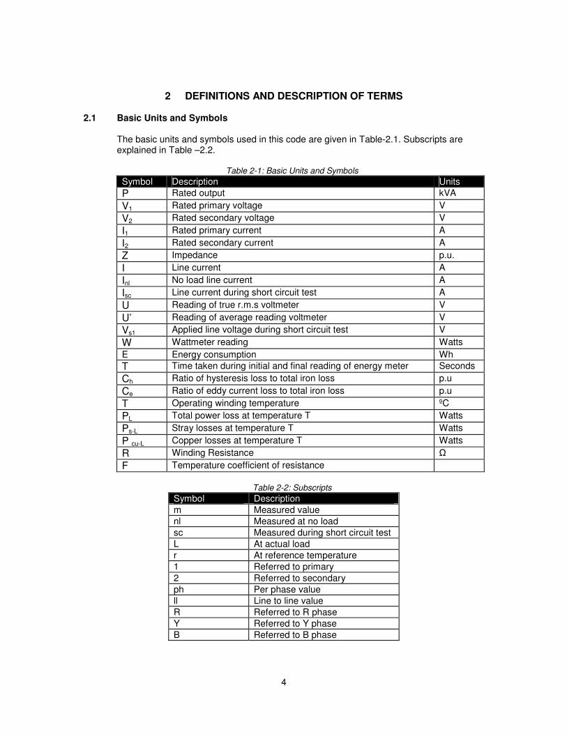
2.1 Basic Units and Symbols The basic units and symbols used in this code are given in Table-2.1. Subscripts are explained in Table –2.2.

Table 2-1: Basic Units and Symbols

Symbol Description Units

P Rated output kVA

V1 Rated primary voltage V

V2 Rated secondary voltage V

I1 Rated primary current A

I2 Rated secondary current A

Z Impedance p.u.

I Line current A

Inl No load line current A

Isc Line current during short circuit test A

U Reading of true r.m.s voltmeter V

U’ Reading of average reading voltmeter V

Vs1 Applied line voltage during short circuit test V

W Wattmeter reading Watts

E Energy consumption Wh

T Time taken during initial and final reading of energy meter Seconds

Ch Ratio of hysteresis loss to total iron loss p.u

Ce Ratio of eddy current loss to total iron loss p.u

T Operating winding temperature ºC

PL Total power loss at temperature T Watts

Ps-L Stray losses at temperature T Watts

P cu-L Copper losses at temperature T Watts

R Winding Resistance Ω

F Temperature coefficient of resistance

Table 2-2: Subscripts

Symbol Description

m Measured value

nl Measured at no load

sc Measured during short circuit test

L At actual load

r At reference temperature

1 Referred to primary

2 Referred to secondary

ph Per phase value

ll Line to line value

R Referred to R phase

Y Referred to Y phase

B Referred to B phase

5

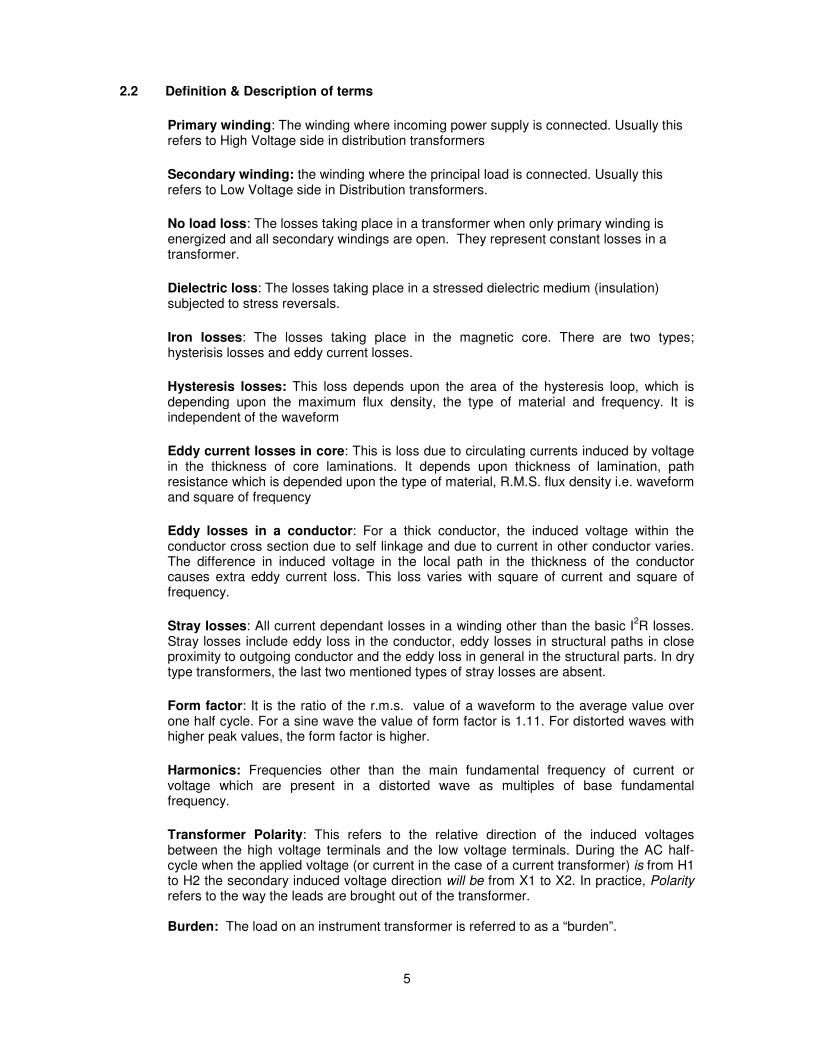
2.2 Definition & Description of terms

Primary winding: The winding where incoming power supply is connected. Usually this refers to High Voltage side in distribution transformers

Secondary winding: the winding where the principal load is connected. Usually this refers to Low Voltage side in Distribution transformers.

No load loss: The losses taking place in a transformer when only primary winding is energized and all secondary windings are open. They represent constant losses in a transformer.

Dielectric loss: The losses taking place in a stressed dielectric medium (insulation) subjected to stress reversals.

Iron losses: The losses taking place in the magnetic core. There are two types; hysterisis losses and eddy current losses.

Hysteresis losses: This loss depends upon the area of the hysteresis loop, which is depending upon the maximum flux density, the type of material and frequency. It is independent of the waveform

Eddy current losses in core: This is loss due to circulating currents induced by voltage in the thickness of core laminations. It depends upon thickness of lamination, path resistance which is depended upon the type of material, R.M.S. flux density i.e. waveform and square of frequency

Eddy losses in a conductor: For a thick conductor, the induced voltage within the conductor cross section due to self linkage and due to current in other conductor varies. The difference in induced voltage in the local path in the thickness of the conductor causes extra eddy current loss. This loss varies with square of current and square of frequency.

Stray losses: All current dependant losses in a winding other than the basic I2R losses.

Stray losses include eddy loss in the conductor, eddy losses in structural paths in close proximity to outgoing conductor and the eddy loss in general in the structural parts. In dry type transformers, the last two mentioned types of stray losses are absent.

Form factor: It is the ratio of the r.m.s. value of a waveform to the average value over one half cycle. For a sine wave the value of form factor is 1.11. For distorted waves with higher peak values, the form factor is higher.

Harmonics: Frequencies other than the main fundamental frequency of current or voltage which are present in a distorted wave as multiples of base fundamental frequency.

Transformer Polarity: This refers to the relative direction of the induced voltages between the high voltage terminals and the low voltage terminals. During the AC half-cycle when the applied voltage (or current in the case of a current transformer) is from H1 to H2 the secondary induced voltage direction will be from X1 to X2. In practice, Polarity refers to the way the leads are brought out of the transformer. Burden: The load on an instrument transformer is referred to as a “burden”.

6

Short circuit impedance & Impedance voltage: The impedance voltage of a transformer is the voltage required to circulate rated current through one of the two specified windings; when the other winding is short circuited with the winding connected as for rated operation. The short circuit impedance is the ratio of voltage and current under above conditions. The resistive component of short circuit impedance, gives a parameter for estimating load losses. These losses include eddy current losses in the conductors and structure as a small portion. Their contribution is materially enhanced due to harmonic currents in load. Exact determination by test is difficult and simplified test at low current suffers from the disadvantage of a high multiplying factor; but it is expected to give representative values.

7

3 GUIDING PRINCIPLES 3.1 Safety precautions

The tests require operation on the HV side of a transformer. Extreme caution should be exercised in consultation with the plant personnel to see that HV system is deactivated and discharged safely prior to access. Similarly while energizing from LV side, the reach of induced HV side voltage should be restricted to prevent damage to personnel/ equipment through inadvertent access.

Some simple minimum steps for ensuring safety are as follows.

1. Qualified engineers should be conducting the test. Safety work permit should be issued to the person.

2. The transformer should be on normal tap

3. Before conducting the tests, the HT area should be clearly demarcated to set up a suitable physical barrier to prevent inadvertent entry /proximity of personnel in the HT zone.

4. The HT supply should be switched off by the primary breaker visibly and then disconnected by the isolator; followed by disconnection on the LT side.

5. The HT side terminals should be discharged by a proper grounding rod, which is compatible with the voltage level on the HT side.

6. The primary terminals should then be physically disconnected and left open.

7. It should be remembered that application of even 4 volts on the secondary LT side can induce more than 100 volts on the 11 kV HT side, as per transformer ratio. Similarly abrupt breaking of relatively small D.C. currents can give large voltage spikes on the HT side.

3.2 Sources of errors and precautions 3.2.1 Ratio and phase angle errors

For no load test, the circuit power factor is very low. (0.05 to 0.15). Hence more sensitive energy meters calibrated for preferably 0.1 or 0.2 pf should be used. Indicating meters should be so selected as to give an indication in 20% to 100% full scale. Digital meters can give more reliable low end readings. Electro-dynamic watt meters have a small angle of lag for the pressure coil circuit by which the pressure coil flux lags the applied circuit voltage. This angle of lag should be added to measured angle like CT phase angle error. Electronic energy meters/watt meters may not have this error. CTs used will have a ratio error within 0.5%. The phase angle of the CT secondary current with respect to real current can be leading by phase angle error ‘cd’ stated in minutes. This error causes a very significant effect on measured power and tends to give a higher reading. It is recommended that the CT’s used should be calibrated to have known ratio and phase angle errors over the working range and for the intended burden of the wattmeter and the ammeter.

8

Recommendations: It is recommended to use portable power analysers or digital energy meters calibrated with CTs of suitable range and the errors be known in the entire current range.

3.3 Estimation of transformer efficiency

The total losses in a transformer at base kVA as well as at the actual load are estimated. From the rated output and measured output, transformer efficiency is calculated as follows.

Efficiency at full load = %100×

+ loadfullatlossesTotaloutputRated

outputRated

. Efficiency at actual load =

%100×

+ loadactualatlossesTotalloadactualatpowerOutput

loadactualatpowerOutput

Considering the fact that distribution transformers are usually operated at around 50% of the rating, estimation of losses at 50% load can also be done by extrapolation method and efficiency at 50% load can be calculated.

9

4 INSTRUMENTS AND METHODS OF MEASUREMENTS 4.1 Measurements/estimation of parameters

The measurements of the following parameters are required for transformer loss estimation. 1. Power input 2. Current 3. Voltage 4. Frequency 5. Winding Resistance 6. Temperature of winding

4.2 Power input

A wattmeter or a suitable electronic 3-phase 4-wire energy meter calibrated for 0.1 p.f can be used for measurement of power in no load test and short circuit test. It also gives a power reading or for improved resolution, energy reading over a period of measured time is possible. Modern digital energy meters have indications of voltage, current, power and frequency; hence more convenient for site measurements. Electronic 3 phase 4 wire energy/power meters of 0-5A range and multiple voltage ranges from 60 V to 500 V with a full-scale indication in the range of 0.1 pf and 0.5-class accuracy is preferred. Separate single phase energy/power meters can be used but a single 3 phase 4- wire energy meter is more convenient.

CT’s of bar primary type 0.5-class accuracy with multiple ranges can be used. The CT's should be calibrated to indicate its ratio error and phase angle error at 10% to 100% current with the specific burden of ammeters and power meters used. During use, the phase angle error is directly taken from the calibration curve for specific current readings. Ratio error can be taken as constant or the nominal ratio can be taken.

4.2.1 No load loss measurements

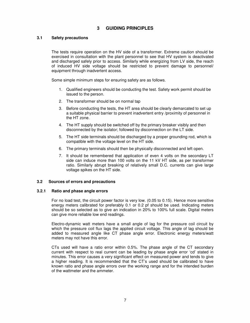
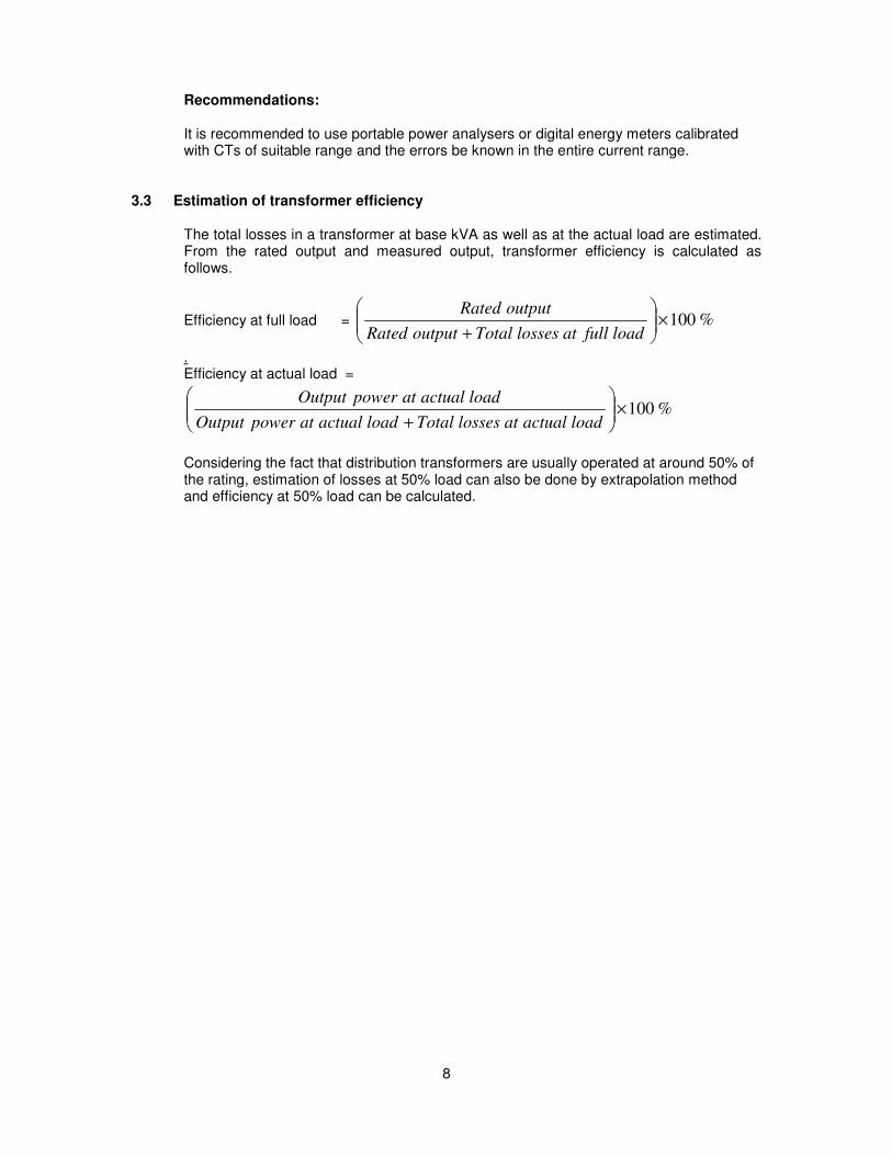
No load losses can be measured from the L.V. side using an adjustable three phase voltage source with neutral. It can be derived from mains or a D.G. set. The voltage and frequency should be steady and at rated values and as near as possible to 50 Hz and it should be measured. This test can give a basic value near rated conditions if all precautions are taken. The L.V. side is energised at the rated tap at rated voltage and power is measured by three watt meters or 3 phase, 4 wire single wattmeter/energy meter. Connections are made as given in figure 4.1 for single phase transformers and figure 4.2 for 3 phase transformers. Due to energisation on L.V. side, PT’s are avoided.

10

Figure 4-1: No load test set up for single phase transformers

R

Y

B

I

VR

R

Y

B

Contactor

3- φ transformer

I

I

VY

N

W2

W3

VB

W1

Total power = W1+W2+W3

Figure 4-2: No load test set up for 3 phase transformers

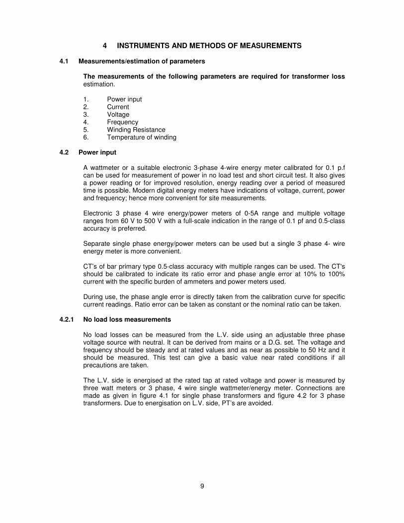
The following figure 4.3 shows connection diagram of a typical 3 phase 4 wire energy metering for measuring energy input to the transformer. All electrical parameters can be monitored using this system.

Figure 4-3: Connection diagram using 3-phase 4 wire energy meter

11

The no load energy consumption, Enl can be measured in the 3 phase – 4 wire meter connected as in figure-4.3. Time taken, t, between initial and final readings are noted. Average no load power is estimated from average energy consumption and time taken.

Average no load power consumption, Wnl ‘ =

Time

nconsumptioenergyAverage

= Wattst

Enl3600×

Where Enl = Energy consumption in at no load during ‘t’ seconds 4.2.2 Load loss Test

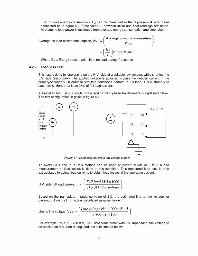
This test is done by energizing on the H.V. side at a suitable low voltage, while shorting the L.V. side (secondary). The applied voltage is adjusted to pass the needed current in the primary/secondary. In order to simulate conditions nearest to full load, it is customary to pass 100%, 50% or at least 25% of full load current. A simplified test using a single phase source for 3 phase transformers is explained below. The test configuration in given in figure 4.4.

Figure 4-4: Load loss test using low voltage supply

To avoid CT’s and PT’s, this method can be used at current levels of 2 to 5 A and measurement of load losses is done at this condition. This measured load loss is then extrapolated to actual load currents to obtain load losses at the operating current.

H.V. side full load current, I1 =

×

×

voltagelineVH

kVAloadFull

..3

1000

Based on the nameplate impedance value of Z%, the estimated line to line voltage for passing 5 A on the H.V. side is calculated as given below.

Line to line voltage, V l-SC =

××

×××

100866.0

51000

1I

ZkVvoltageLine

For example, for a 11 kV/433 V, 1000 kVA transformer with 5% impedance, the voltage to be applied on H.V. side during load test is estimated below.

12

H.V. side full load current, I1 =

×

×

voltagelineVH

kVAloadFull

..3

1000

=

×

×

110003

10001000

= 52.5 A

Line to line voltage to be applied on H.V side for getting 5 A on H.V. side,

V l-SC =

××

×××

100866.0

51000

1I

ZkVvoltageLine

=

××

×××

1005.52866.0

55100011

= 60.5 volts

The test is repeated thrice, taking terminals HR and HY by applying voltage ERY and then HY and HB with EYB and then HR and HB applying voltage ERB. The power readings with corrections are PRY, PYB and PRB respectively. Current drawn on H.V. side I s1 is also noted.

Since the current drawn on H.V. side is only about 5A in this test, CT’s can be avoided and hence phase angle error is not applicable.

Measured load loss, Wsc = 5.13

×

++ RBYBRY PPP

Since the test voltage is low iron losses are negligible. The measured power input represents the resistive losses in the windings and stray losses.

4.2.3 Operating load measurements

This measurement is to be carried out after a sustained load level for 3 to 4 hours. The Frequency, Voltage, Current and Power should be measured at L.T side using calibrated 0.5 class meters of suitable range. Note that p.f. at actual load conditions may vary from 0.7 to 1.0 and power meters should be calibrated in this range. The power measured at the L.T side will give the output power of the transformer.

4.3 Voltage

Two types of voltmeters are used in the measurements.

1. Average reading type voltmeters with scale calibrated assuming the normal form factor of 1.11 for sine wave. The usual digital voltmeters are of this variety.

2. R.M.S. reading voltmeter, preferably digital true r.m.s meters are the second type.

Digital electronic instrument with usual a.c range calibrated for sine wave is used for Average reading voltage measurement. For true r.m.s reading a digital electronic meter of true r.m.s type with a 600v/750v range is recommended of 0.5 class accuracy.

13

4.3.1 Waveform errors

Ideally, the no load loss is to be measured at the rated maximum flux density and sinusoidal flux variation, at rated frequency. This means that during no load test, an adjustable voltage supply would be required to vary the applied voltage to get the rated flux density. Applied voltage = Rated voltage x actual frequency Rated frequency

To account for the distortion in waveforms, which is usually seen in waveforms, which may be present during measurements, the values of average and r.m.s voltages are to be measured across the transformer phase windings. The r.m.s. voltage U may slightly higher than average voltage U’. The measured core losses need to be corrected to sinusoidal excitation, by using the following expression.

No load losses corrected for sinusoidal excitation, Wnl = ( )eh

mnl

kCC

W

+−

Where k = form factor correction =

'U

U 2

Ch = Ratio of hysteresis loss to total iron losses Ce = Ratio of eddy current losses to total iron losses

For usual flux densities, the following data can be used. For oriented steel, Ch = Ce = 0.5 For non-oriented steel , Ch = 0.7, Ce = 0.3 For amorphous core materials, Wnl = Wnl-m

4.4 Frequency

A digital frequency-measuring instrument for 50 Hz range with 600v range and having a resolution of 0.1 Hz is preferred.

4.5 Winding temperature

The transformer should be de-energised with continued cooling for at least 8 hours. Alternatively, if the winding temperature does not vary by more than 1ºC over a period of 30 minutes, the transformer can be assumed to have reached a cold stage. For oil cooled transformers, the temperature can be measured either at the top of the oil surface or in an oil filled thermo-well if it is provided. For dry type transformers, the temperature sensor should be kept in close contact with coil surface. The sensor should be covered and protected from direct draft. When a stable temperature is reached in the indicator, within 1ºC, this temperature is taken as temperature of the windings, Tm, at the time of measuring the winding resistance. For oil temperature measurements calibrated mercury in glass thermometer can be used with a resolution of 1ºC .in general, electronic instruments with suitable probes are preferred. They include probes using thermo couple resistance or Thermisters with the resolution of 1ºC.

14

For surface temperature measurements the probe of the instrument should be mounted and covered suitably. Due care should be taken to isolate the instrument for reliable reading and safety

4.6 Cold winding resistance

The winding resistance can be measured using a Kelvin bridge for low resistances or a wheat-stone bridge for resistances above 10 Ω. It is preferable to use modern direct reading digital resistance measuring instruments with a resolution of 10 micro Ω or better for L.V. windings.

If resistance is measured across line terminals, the per phase resistance can be calculated as follows: 1. If winding is connected in delta, Rph = 1.5 x Rll 2. If winding is connected in Star, Rph = 0.5 x Rll The value of the resistance for primary and secondary windings as measured should be corrected to a standard temperature of 75 ºC by using the following expression.

+

+×= −

FT

FTRR

m

mphph

Where R ph = Resistance at temperature T, Ω R ph-m = Resistance measured at measured winding temperature Tm, Ω T = Winding temperature, ºC at which resistance is to be referred Tm = Temperature of winding at the time of resistance measurement, ºC F = Temperature coefficient. = 235 for copper = 225 for Aluminium = 230 for alloyed Aluminium

Thus, for copper windings,

+

+×=

235

235

m

rmr

T

TRR

For low resistance measurements an electronic, four terminal digital instruments is preferred with a minimum accuracy of 10 micro ohms. Note: The micro ohmmeters generally inject 1.0 ampere current to the winding while measuring resistance. For transformers rated above 100 kVA, this current may not be sufficient to give appreciable voltages for the instrument to measure. Hence a DC current generator capable of supplying about 5 Amp may be required.

4.6.1 Settling time for readings

Due to circuit time constant, for the current driving circuit used, final reading will take some time for reaching a stable value. This time should be measured and noted. This time is useful for taking a valid reading when taking hot winding resistance. If hot resistance is measured after de-energising the transformer, a valid reading can only be considered after the lapse of settling time as measured above.

15

Polarity of D.C. current with respect to winding terminals should be consistently same. The above comment is applicable to all resistance measurements including those taken by bridge method or using a direct indicating digital meter.

16

5 COMPUTATION OF RESULTS 5.1 Sequence of Tests

Any convenient sequence can be followed, but preferably after a sufficiently long OFF period, the test for cold winding resistance should be taken first to minimise minor temperature rise errors. This should be followed by no load loss test and then followed by short circuit test, if needed. Indirect or direct measurement of operating winding temperature can be planned and taken after a proper stabilization period under any chosen load condition. Measurement of actual operating parameters also needs to be done during normal load condition.

5.2 Chronological order of measurements and calculations

1. Obtain nameplate specifications of the transformer. 2. Switch off the transformer for at least 8 hours with continued cooling to attain steady

state. Alternatively, measure winding temperature at every 15 minutes and if temperature drop is not more than 1ºC, the transformer can be considered to have attained steady state.

3. Measure resistances of primary and secondary windings. If resistance is measured across line terminals, the per phase resistance can be calculated as follows:

If winding is connected in delta, Rph = 1.5 x Rll If winding is connected in Star, Rph = 0.5 x Rll

4. Conduct no load test, by energizing on the L.V. side. For this, first connect instruments as in figure 4.3 for single phase transformers or as in figure 4.1 for three phase transformers.

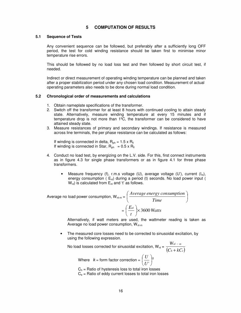
• Measure frequency (f), r.m.s voltage (U), average voltage (U’), current (Inl), energy consumption ( Enl) during a period (t) seconds. No load power input ( Wnl) is calculated from Enl and ‘t’ as follows.

Average no load power consumption, Wnl-m =

Time

nconsumptioenergyAverage

= Wattst

Enl3600×

Alternatively, if watt meters are used, the wattmeter reading is taken as Average no load power consumption, Wnl-m

• The measured core losses need to be corrected to sinusoidal excitation, by using the following expression.

No load losses corrected for sinusoidal excitation, Wnl = ( )eh

mnl

kCC

W

+

−

Where k = form factor correction =

'U

U 2

Ch = Ratio of hysteresis loss to total iron losses Ce = Ratio of eddy current losses to total iron losses

17

For usual flux densities, the following data can be used. For oriented steel, Ch = Ce = 0.5 For non-oriented steel, Ch = 0.7, Ce = 0.3 For amorphous core materials, Wnl = Wnl-m

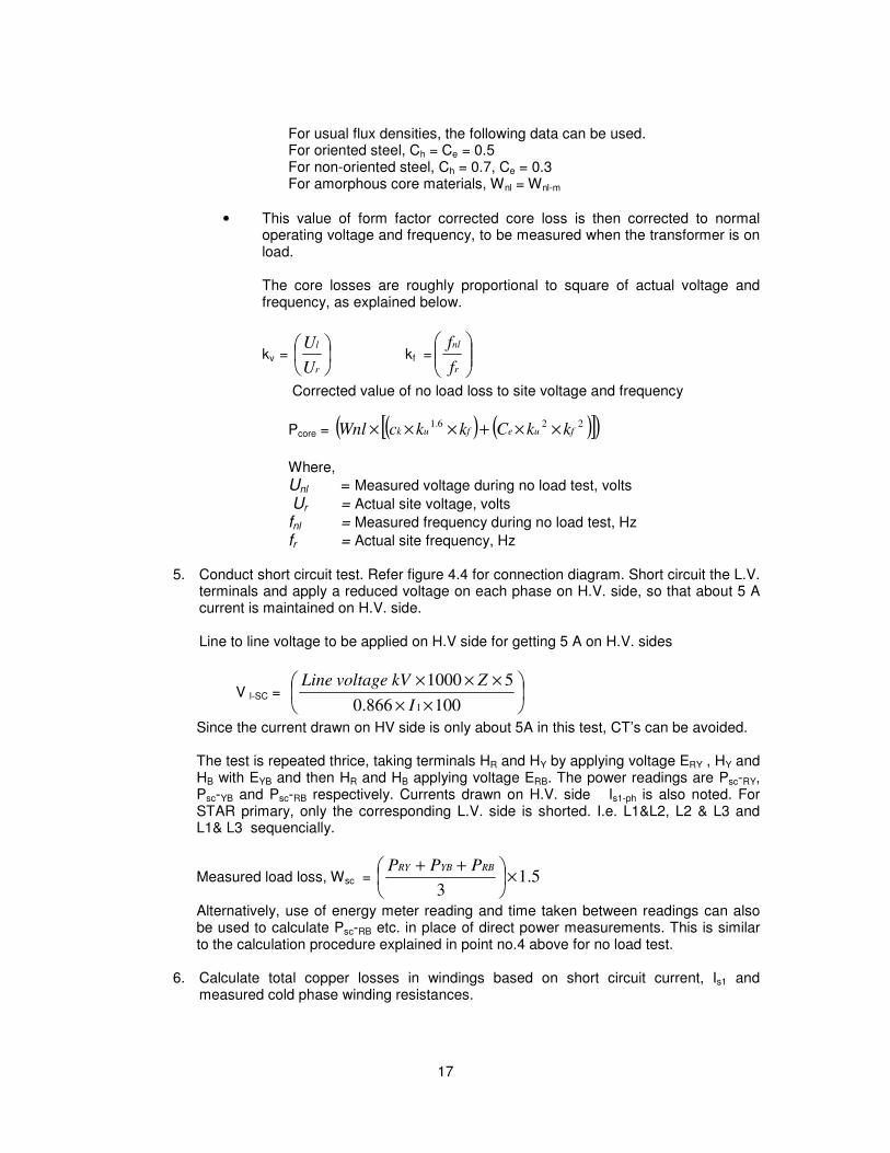
• This value of form factor corrected core loss is then corrected to normal operating voltage and frequency, to be measured when the transformer is on load.

The core losses are roughly proportional to square of actual voltage and frequency, as explained below.

kv =

r

l

U

U kf =

r

nl

f

f

Corrected value of no load loss to site voltage and frequency

Pcore = ( ) ( )[ ]( )226.1fuefuk kkCkkcWnl ××+×××

Where,

Unl = Measured voltage during no load test, volts

Ur = Actual site voltage, volts

fnl = Measured frequency during no load test, Hz

fr = Actual site frequency, Hz 5. Conduct short circuit test. Refer figure 4.4 for connection diagram. Short circuit the L.V.

terminals and apply a reduced voltage on each phase on H.V. side, so that about 5 A current is maintained on H.V. side.

Line to line voltage to be applied on H.V side for getting 5 A on H.V. sides

V l-SC =

××

×××

100866.0

51000

1I

ZkVvoltageLine

Since the current drawn on HV side is only about 5A in this test, CT’s can be avoided.

The test is repeated thrice, taking terminals HR and HY by applying voltage ERY , HY and HB with EYB and then HR and HB applying voltage ERB. The power readings are Psc-RY, Psc-YB and Psc-RB respectively. Currents drawn on H.V. side Is1-ph is also noted. For STAR primary, only the corresponding L.V. side is shorted. I.e. L1&L2, L2 & L3 and L1& L3 sequencially.

Measured load loss, Wsc = 5.13

×

++ RBYBRY PPP

Alternatively, use of energy meter reading and time taken between readings can also be used to calculate Psc-RB etc. in place of direct power measurements. This is similar to the calculation procedure explained in point no.4 above for no load test.

6. Calculate total copper losses in windings based on short circuit current, Is1 and measured cold phase winding resistances.

18

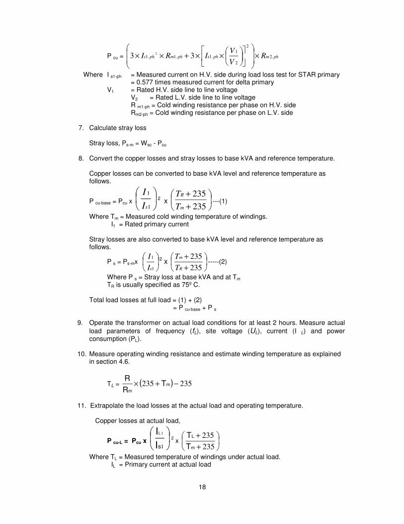
P cu = phmphsphmphs RV

VIRI .2

2

2

1

.1.1.1 332 ×

××+××

Where I s1-ph = Measured current on H.V. side during load loss test for STAR primary = 0.577 times measured current for delta primary V1 = Rated H.V. side line to line voltage V2 = Rated L.V. side line to line voltage R m1-ph = Cold winding resistance per phase on H.V. side Rm2-ph = Cold winding resistance per phase on L.V. side

7. Calculate stray loss Stray loss, Ps-m = Wsc - Pcu

8. Convert the copper losses and stray losses to base kVA and reference temperature.

Copper losses can be converted to base kVA level and reference temperature as follows.

P cu-base = Pcu x

1

1

sI

I2 x

+

+

235

235

m

R

T

T---(1)

Where Tm = Measured cold winding temperature of windings. I1 = Rated primary current Stray losses are also converted to base kVA level and reference temperature as follows.

P s = Ps-mx

1

1

sI

I 2 x

+

+

235

235

R

m

T

T-----(2)

Where P s = Stray loss at base kVA and at Tm TR is usually specified as 75º C.

Total load losses at full load = (1) + (2)

= P cu-base + P s

9. Operate the transformer on actual load conditions for at least 2 hours. Measure actual

load parameters of frequency (fL), site voltage (UL), current (I L) and power consumption (PL).

10. Measure operating winding resistance and estimate winding temperature as explained

in section 4.6.

TL = ( ) 235235 −+× m

m

TR

R

11. Extrapolate the load losses at the actual load and operating temperature.

Copper losses at actual load,

P cu-L = Pcu x

1

1

sI

IL

2 x

+

+

235

235

m

L

T

T

Where TL = Measured temperature of windings under actual load. IL = Primary current at actual load

19

IL1 can also be estimated from secondary current at actual load, I2 by using transformer voltage ratio.

IL1 =

×1

2

2

V

VIL

IL2 = Secondary current at actual load Stray losses at actual load,

P sL = Ps-mx

1

1

s

L

I

I 2 x

+

+

235

235

L

m

T

T-----(2)

Where P sL = Stray loss at actual load

12. Estimation of transformer efficiency

The above steps calculates total losses in a transformer at base kVA as well as at the actual load.

Efficiency at full load, ηFL = ( )%100×

+ loadfullatlossesTotaloutputRated

outputRated

= ( )scucore PPPP

P

+++×

×

1000

1000x 100

Efficiency at actual load, η L =

( )%100×

+ loadactualatlossesTotalloadactualatpowerOutput

loadactualatpowerOuput

= ( )scucoreL

L

PPPP

P

+++×

×

1000

1000x 100 %

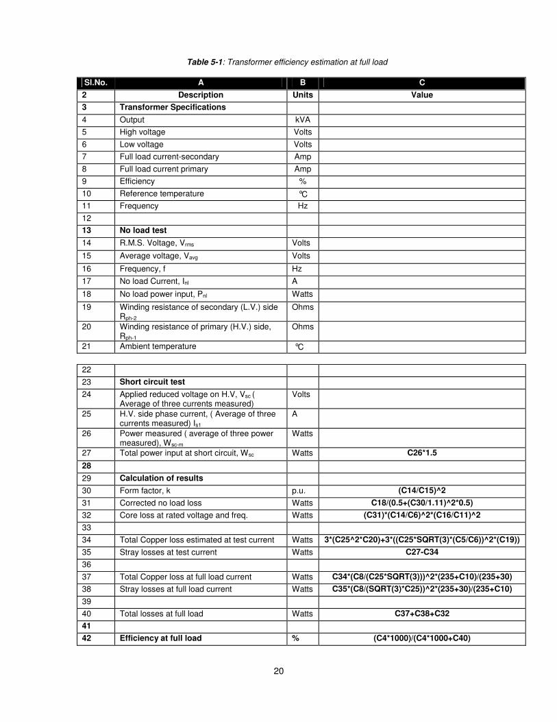
Table 5.1 shows the calculations for estimating transformer efficiency at full load with MS

Excel programmable equations.

20

Table 5-1: Transformer efficiency estimation at full load

Sl.No. A B C

2 Description Units Value

3 Transformer Specifications

4 Output kVA

5 High voltage Volts

6 Low voltage Volts

7 Full load current-secondary Amp

8 Full load current primary Amp

9 Efficiency %

10 Reference temperature °C

11 Frequency Hz

12

13 No load test

14 R.M.S. Voltage, Vrms Volts

15 Average voltage, Vavg Volts

16 Frequency, f Hz

17 No load Current, Inl A

18 No load power input, Pnl Watts

19 Winding resistance of secondary (L.V.) side Rph-2

Ohms

20 Winding resistance of primary (H.V.) side, Rph-1

Ohms

21 Ambient temperature °C

22

23 Short circuit test

24 Applied reduced voltage on H.V, Vsc ( Average of three currents measured)

Volts

25 H.V. side phase current, ( Average of three currents measured) Is1

A

26 Power measured ( average of three power measured), Wsc-m

Watts

27 Total power input at short circuit, Wsc Watts C26*1.5

28

29 Calculation of results

30 Form factor, k p.u. (C14/C15)^2

31 Corrected no load loss Watts C18/(0.5+(C30/1.11)^2*0.5)

32 Core loss at rated voltage and freq. Watts (C31)*(C14/C6)^2*(C16/C11)^2

33

34 Total Copper loss estimated at test current Watts 3*(C25^2*C20)+3*((C25*SQRT(3)*(C5/C6))^2*(C19))

35 Stray losses at test current Watts C27-C34

36

37 Total Copper loss at full load current Watts C34*(C8/(C25*SQRT(3)))^2*(235+C10)/(235+30)

38 Stray losses at full load current Watts C35*(C8/(SQRT(3)*C25))^2*(235+30)/(235+C10)

39

40 Total losses at full load Watts C37+C38+C32

41

42 Efficiency at full load % (C4*1000)/(C4*1000+C40)

21

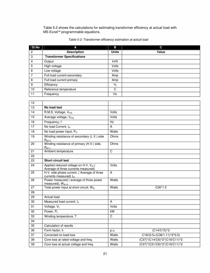
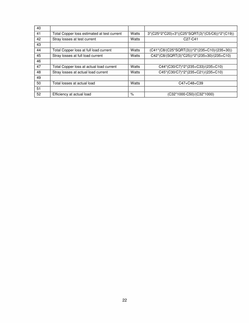
Table 5.2 shows the calculations for estimating transformer efficiency at actual load with

MS Excel programmable equations.

Table 5-2: Transformer efficiency estimation at actual load

Sl.No A B C

2 Description Units Value

3 Transformer Specifications

4 Output kVA

5 High voltage Volts

6 Low voltage Volts

7 Full load current-secondary Amp

8 Full load current primary Amp

9 Efficiency %

10 Reference temperature C

11 Frequency Hz

12

13 No load test

14 R.M.S. Voltage, Vrms Volts

15 Average voltage, Vavg Volts

16 Frequency, f Hz

17 No load Current, Inl A

18 No load power input, Pnl Watts

19 Winding resistance of secondary (L.V.) side Rph-2

Ohms

20 Winding resistance of primary (H.V.) side, Rph-1

Ohms

21 Ambient temperature C

22

23 Short circuit test

24 Applied reduced voltage on H.V, Vsc ( Average of three currents measured)

Volts

25 H.V. side phase current, ( Average of three currents measured) Is1

A

26 Power measured ( average of three power measured), Wsc-m

Watts

27 Total power input at short circuit, Wsc Watts C26*1.5

28

29 Actual load

30 Measured load current, IL A

31 Voltage, VL Volts

32 Power, PL kW

33 Winding temperature, T C

34

35 Calculation of results

36 Form factor, k p.u. (C14/C15)^2

37 Corrected no load loss Watts C18/(0.5+(C36/1.11)^2*0.5)

38 Core loss at rated voltage and freq. Watts (C37)*(C14/C6)^2*(C16/C11)^2

39 Core loss at actual voltage and freq. Watts (C37)*(C31/C6)^2*(C16/C11)^2

22

40

41 Total Copper loss estimated at test current Watts 3*(C25^2*C20)+3*((C25*SQRT(3)*(C5/C6))^2*(C19))

42 Stray losses at test current Watts C27-C41

43

44 Total Copper loss at full load current Watts (C41*(C8/(C25*SQRT(3)))^2*(235+C10)/(235+30))

45 Stray losses at full load current Watts C42*(C8/(SQRT(3)*C25))^2*(235+30)/(235+C10)

46

47 Total Copper loss at actual load current Watts C44*(C30/C7)^2*(235+C33)/(235+C10)

48 Stray losses at actual load current Watts C45*(C30/C7)^2*(235+C21)/(235+C10)

49

50 Total losses at actual load Watts C47+C48+C39

51

52 Efficiency at actual load % (C32*1000-C50)/(C32*1000)

23

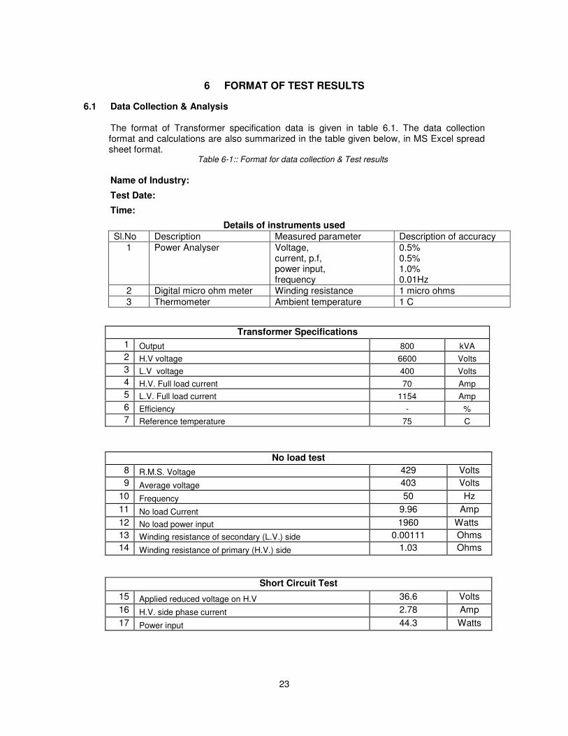
6 FORMAT OF TEST RESULTS

6.1 Data Collection & Analysis

The format of Transformer specification data is given in table 6.1. The data collection format and calculations are also summarized in the table given below, in MS Excel spread sheet format.

Table 6-1:: Format for data collection & Test results

Name of Industry:

Test Date:

Time:

Details of instruments used

Sl.No Description Measured parameter Description of accuracy

1 Power Analyser Voltage, current, p.f, power input, frequency

0.5% 0.5% 1.0% 0.01Hz

2 Digital micro ohm meter Winding resistance 1 micro ohms

3 Thermometer Ambient temperature 1 C

Transformer Specifications

1 Output 800 kVA

2 H.V voltage 6600 Volts

3 L.V voltage 400 Volts

4 H.V. Full load current 70 Amp

5 L.V. Full load current 1154 Amp

6 Efficiency - %

7 Reference temperature 75 C

No load test

8 R.M.S. Voltage 429 Volts

9 Average voltage 403 Volts

10 Frequency 50 Hz

11 No load Current 9.96 Amp

12 No load power input 1960 Watts

13 Winding resistance of secondary (L.V.) side 0.00111 Ohms

14 Winding resistance of primary (H.V.) side 1.03 Ohms

Short Circuit Test

15 Applied reduced voltage on H.V 36.6 Volts

16 H.V. side phase current 2.78 Amp

17 Power input 44.3 Watts

24

Test conducted by: (Energy Auditing Firm) Test witnessed by: (Energy Manager)

Results

19 Core loss at rated voltage and freq. 2207.88 Watts

20 Copper loss at full load 11100.69 Watts

21 Stray losses at full load 3893.24 Watts

22 Total losses at full load 17201.82 Watts

23 Efficiency at full load 97.9 %

24 Uncertainty 0.03 %

25

7 UNCERTAINTY ANALYSIS

7.1 Introduction Uncertainty denotes the range of error, i.e. the region in which one guesses the error to

be. The purpose of uncertainty analysis is to use information in order to quantify the amount of confidence in the result. The uncertainty analysis tells us how confident one should be in the results obtained from a test.

Guide to the Expression of Uncertainty in Measurement (or GUM as it is now often

called) was published in 1993 (corrected and reprinted in 1995) by ISO. The focus of the ISO Guide or GUM is the establishment of "general rules for evaluating and expressing uncertainty in measurement that can be followed at various levels of accuracy “.

The following methodology is a simplified version of estimating combined uncertainty at

field conditions, based on GUM.

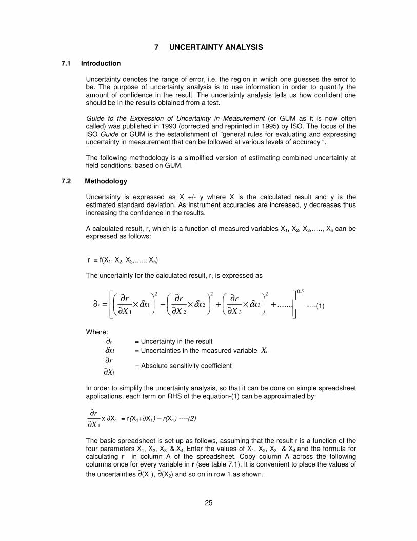
7.2 Methodology

Uncertainty is expressed as X +/- y where X is the calculated result and y is the estimated standard deviation. As instrument accuracies are increased, y decreases thus increasing the confidence in the results.

A calculated result, r, which is a function of measured variables X1, X2, X3,….., Xn can be expressed as follows: r = f(X1, X2, X3,….., Xn) The uncertainty for the calculated result, r, is expressed as

5.02

3

3

2

2

2

2

1

1

.......

+

×∂

∂+

×∂

∂+

×∂

∂=∂ x

X

rx

X

rx

X

rr δδδ ----(1)

Where:

r∂ = Uncertainty in the result

xiδ = Uncertainties in the measured variable iX

iX

r

∂∂

= Absolute sensitivity coefficient

In order to simplify the uncertainty analysis, so that it can be done on simple spreadsheet applications, each term on RHS of the equation-(1) can be approximated by:

1X

r

∂

∂x ∂X1 = r(X1+∂X1) – r(X1) ----(2)

The basic spreadsheet is set up as follows, assuming that the result r is a function of the four parameters X1, X2, X3 & X4. Enter the values of X1, X2, X3 & X4 and the formula for calculating r in column A of the spreadsheet. Copy column A across the following columns once for every variable in r (see table 7.1). It is convenient to place the values of

the uncertainties ∂(X1), ∂(X2) and so on in row 1 as shown.

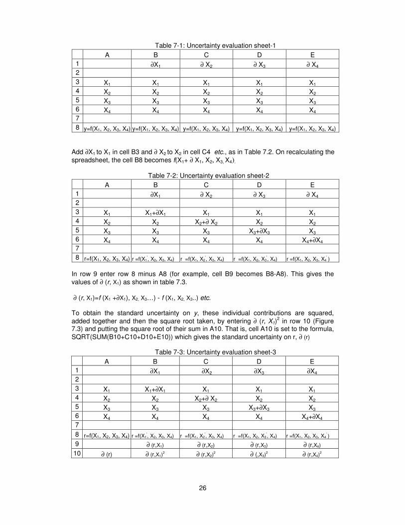
26

Table 7-1: Uncertainty evaluation sheet-1

A B C D E

1 ∂X1 ∂ X2 ∂ X3 ∂ X4

2

3 X1 X1 X1 X1 X1

4 X2 X2 X2 X2 X2

5 X3 X3 X3 X3 X3

6 X4 X4 X4 X4 X4

7

8 y=f(X1, X2, X3, X4) y=f(X1, X2, X3, X4) y=f(X1, X2, X3, X4) y=f(X1, X2, X3, X4) y=f(X1, X2, X3, X4)

Add ∂X1 to X1 in cell B3 and ∂ X2 to X2 in cell C4 etc., as in Table 7.2. On recalculating the

spreadsheet, the cell B8 becomes f(X1+ ∂ X1, X2, X3, X4).

Table 7-2: Uncertainty evaluation sheet-2

A B C D E

1 ∂X1 ∂ X2 ∂ X3 ∂ X4

2

3 X1 X1+∂X1 X1 X1 X1

4 X2 X2 X2+∂ X2 X2 X2

5 X3 X3 X3 X3+∂X3 X3

6 X4 X4 X4 X4 X4+∂X4

7

8 r=f(X1, X2, X3, X4) r =f(X1', X2, X3, X4) r =f(X1, X2

', X3, X4) r =f(X1, X2, X3

', X4) r =f(X1, X2, X3, X4

' )

In row 9 enter row 8 minus A8 (for example, cell B9 becomes B8-A8). This gives the

values of ∂ (r, X1) as shown in table 7.3.

∂ (r, X1)=f (X1 +∂X1), X2, X3…) - f (X1, X2, X3..) etc. To obtain the standard uncertainty on y, these individual contributions are squared,

added together and then the square root taken, by entering ∂ (r, X1)2 in row 10 (Figure

7.3) and putting the square root of their sum in A10. That is, cell A10 is set to the formula,

SQRT(SUM(B10+C10+D10+E10)) which gives the standard uncertainty on r, ∂ (r)

Table 7-3: Uncertainty evaluation sheet-3

A B C D E

1 ∂X1 ∂X2 ∂X3 ∂X4

2

3 X1 X1+∂X1 X1 X1 X1

4 X2 X2 X2+∂ X2 X2 X2

5 X3 X3 X3 X3+∂X3 X3

6 X4 X4 X4 X4 X4+∂X4

7

8 r=f(X1, X2, X3, X4) r =f(X1', X2, X3, X4) r =f(X1, X2

', X3, X4) r =f(X1, X2, X3

', X4) r =f(X1, X2, X3, X4

' )

9 ∂ (r,X1) ∂ (r,X2) ∂ (r,X3) ∂ (r,X4)

10 ∂ (r) ∂ (r,X1)2 ∂ (r,X2)

2 ∂ (,X3)

2 ∂ (r,X4)

2

27

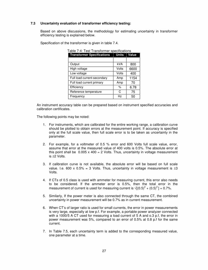
7.3 Uncertainty evaluation of transformer efficiency testing: Based on above discussions, the methodology for estimating uncertainty in transformer efficiency testing is explained below. Specification of the transformer is given in table 7.4.

Table 7-4: Test Transformer specifications

Transformer Specifications Units Value

Output kVA 800

High voltage Volts 6600

Low voltage Volts 400

Full load current-secondary Amp 1154

Full load current primary Amp 70

Efficiency % 6.78

Reference temperature C 75

Frequency Hz 50

An instrument accuracy table can be prepared based on instrument specified accuracies and calibration certificates. The following points may be noted:

1. For instruments, which are calibrated for the entire working range, a calibration curve should be plotted to obtain errors at the measurement point. If accuracy is specified only at the full scale value, then full scale error is to be taken as uncertainty in the parameter.

2. For example, for a voltmeter of 0.5 % error and 600 Volts full scale value, error,

assume that error at the measured value of 400 volts is 0.5%. The absolute error at this point shall be 0.005 x 400 = 2 Volts. Thus, uncertainty in voltage measurement

is ±2 Volts.

3. If calibration curve is not available, the absolute error will be based on full scale

value. I.e. 600 x 0.5% = 3 Volts. Thus, uncertainty in voltage measurement is ±3 Volts.

4. If CTs of 0.5 class is used with ammeter for measuring current, this error also needs

to be considered. If the ammeter error is 0.5%, then the total error in the

measurement of current is used for measuring current is √[(0.5)2 + (0.5)

2 ] = 0.7%.

5. Similarly, If the power meter is also connected through the same CT, the combined

uncertainty in power measurement will be 0.7% as in current measurement.

6. When CT’s of larger ratio is used for small currents, the error in power measurements is very large, especially at low p.f. For example, a portable power analyzer connected with a 1000/5 A CT used for measuring a load current of 5 A and o.3 p.f, the error in power measurement was 5%, compared to an error of 0.5% at 0.8 p.f for the same current.

7. In Table 7.5, each uncertainty term is added to the corresponding measured value,

one parameter at a time.

28

Table 7-5: Uncertainty Evaluation δ δ δ δ Vrms δδδδVavg δδδδf δδδδInl δδδδWnl δδδδRph-2 δδδδRph-1 δδδδVsc δδδδIs1 δδδδWsc

If % accuracy is known at operating point, enter % value in this row

Units % acc. 0.50% 0.50% 1.00% 5.00% 0.50% 0.50% 0.5% 1.0% 5.0%

If % accuracy is known at full scale only, calculate full scale error and enter actual value in this row

value 2.15 2.02 0.01 0.10 98.0 0.000006 0.0052 0.183 0.0278 3.32250

No load test

R.M.S. Voltage, Vrms Volts 429.0 431.1 429.0 429.0 429.0 429.0 429.0 429.0 429.0 429.0 429.0

Average voltage, Vavg Volts 403 403.00 405.02 403.00 403.00 403.00 403.00 403.00 403.00 403.00 403.00

Frequency, f Hz 50 50.00 50.00 50.01 50.00 50.00 50.00 50.00 50.00 50.00 50.00

No load Current, Inl A 9.96 9.96 9.96 9.96 10.1 9.96 9.96 9.96 9.96 9.96 9.96

No load power input, Pnl Watts 1960 1960 1960 1960 1960 2058.0 1960 1960 1960 1960 1960

Winding resistance of secondary (L.V.) side Rph-2

Ohms 0.00111 0.00111 0.00111 0.00111 0.00111 0.00111 0.001116 0.00111 0.00111 0.00111 0.00111

Winding resistance of primary (H.V.) side, Rph-1

Ohms 1.0300 1.0300 1.0300 1.0300 1.0300 1.0300 1.0300 1.0352 1.0300 1.0300 1.0300

Ambient temperature 30.0

Short circuit test

Applied reduced voltage on H.V, Vsc ( Average of three currents measured)

Volts 36.60 36.60 36.60 36.60 36.60 36.60 36.60 36.60 36.78 36.60 36.60

H.V. side phase current, ( Average of three currents measured) Is1

A 2.78 2.78 2.78 2.78 2.78 2.78 2.78 2.78 2.78 2.81 2.78

Power measured ( average of three power measured), Wsc-m

Watts 44.30 44.30 44.30 44.30 44.30 44.30 44.30 44.30 44.30 44.30 44.30

Total power input at short circuit, Wsc Watts 66.45 66.45 66.45 66.45 66.45 66.45 66.45 66.45 66.45 66.45 66.45

Calculation of results

Form factor, k p.u. 1.1332 1.1446 1.1219 1.1332 1.1332 1.1332 1.1332 1.1332 1.1332 1.1332 1.1332

Corrected no load loss Watts 1919.47 1899.93 1939.02 1919.47 1919.47 2015.45 1919.47 1919.47 1919.47 1919.47 1919.47

Core loss at rated voltage and freq. Watts 2207.88 2207.32 2230.37 2208.77 2207.88 2318.28 2207.88 2207.88 2207.88 2207.88 2207.88

Total Copper loss estimated at test current

Watts 44.90 44.90 44.90 44.90 44.90 44.90 45.01 45.02 44.90 45.80 44.90

Stray losses at test current Watts 21.55 21.55 21.55 21.55 21.55 21.55 21.44 21.43 21.55 20.65 21.55

Total Copper loss at full load current Watts 11100.69 11100.69 11100.69 11100.69 11100.69 11100.69 11126.68 11130.21 11100.69 11100.69 11100.69

Stray losses at full load current Watts 3893.24 3893.24 3893.24 3893.24 3893.24 3893.24 3874.25 3871.67 3893.24 3656.69 3893.24

Total losses at full load Watts 17201.82 17201.25 17224.30 17202.70 17201.82 17312.21 17208.81 17209.76 17201.82 16965.27 17201.82

Efficiency at full load % 97.90% 97.90% 97.89% 97.89% 97.90% 97.88% 97.89% 97.89% 97.90% 97.92% 97.90%

29

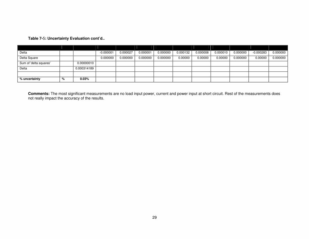
Table 7-5: Uncertainty Evaluation cont’d..

Delta -0.000001 0.000027 0.000001 0.000000 0.000132 0.000008 0.000010 0.000000 -0.000283 0.000000

Delta Square 0.000000 0.000000 0.000000 0.000000 0.00000 0.00000 0.00000 0.000000 0.00000 0.000000

Sum of 'delta squares' 0.00000010

Delta 0.000314189

% uncertainty % 0.03%

Comments: The most significant measurements are no load input power, current and power input at short circuit. Rest of the measurements does not really impact the accuracy of the results.

30

8 GUIDELINES FOR ENERGY CONSERVATION OPPORTUNITIES

The following points have to be considered.

1. Power factor correction for reducing copper losses.

2. System operating voltages to be observed for maintaining near rated voltages and unbalanced to be minimized.

3. Augmented cooling and relative benefits to be seen where applicable.

4. Possibility of switching off paralleled transformers at any low loads.

5. Working out existing realistic losses and cost thereof. This follows study of annual r.m.s. loading and operating losses at operating temperature, covering harmonic loading. This is a prerequisite for finding replacement alternatives.

6. Replacement by a low loss transformer with economic justification, considering present and future harmonic loading and load pattern.

7. When replacement is not justified, collection of invited/standard low loss design data for optimum cost/rating of transformer for future replacement or for new installation.

31

ANNEXURE 1: EFFECT OF HARMONICS A1.1 Effect of current harmonics on load losses A1.2 Introduction

The load losses consist of normal I2R losses in the conductor and the stray losses due to

eddy currents in thick conductors due to varying induced voltage within the cross section of the conductor due to self linkages and due to currents in near by current carrying conductors. These induced voltages circulate eddy current in the local loop. In oil cooled transformers, the heavy current output conductors have proximity to structural parts wherein eddy losses can take place. Similarly, some stray flux can in general cause eddy losses in structural parts. The distribution of stray losses in the two last named categories can be estimated by design experience. It can not be directly measured.

Thus load losses = I

2RDC + I

2Rextra Eddy in windings + I

2Rextra eddy in structure near out

going conductors + I2Rextra Eddy in Tank Structure

The last three are clubbed together and distribution is assumed 90% and 10%. In general, the eddy losses are materially increased since they vary as per square of frequency. Effects of the triplens ( 3

rd, 9

th etc.) is to cause circulating currents which circulate in delta

winding causing added losses. They also add up in neutral connection and conductor causing extra heating and losses. In general, harmonic order h = p (pulse number) x K + 1 where K = 1 to n. Accordingly six pulse converters give 5,7,11,13,……. Twelve pulse converters give 11,13,………

The application problems are of two types.

a) How to specify the transformer for a general mix of active loads. b) How to estimate extra losses when current harmonics are known for an existing

transformer.

A1.4 U.S. Practices – K- Factor

The K-Factor rating assigned to a transformer and marked on the transformer case in accordance with the listing of Underwriters Laboratories, is an index of the transformer's ability to supply harmonic content in its load current while remaining within its operating temperature limits. For specification in general, the U.S. practice is to estimate the K – Factor which gives ready reference ratio K for eddy losses which driving non linear loads as compared to linear loads.

h

K = Σ Ih2H

2

1 K = 1 for Resistance heating motors, distribution transformers etc. K = 4 for welders Induction heaters, Fluorescent lights K = 13 For Telecommunication equipment. K = 20 For main frame computers, variable speed drives and desktop computers.

32

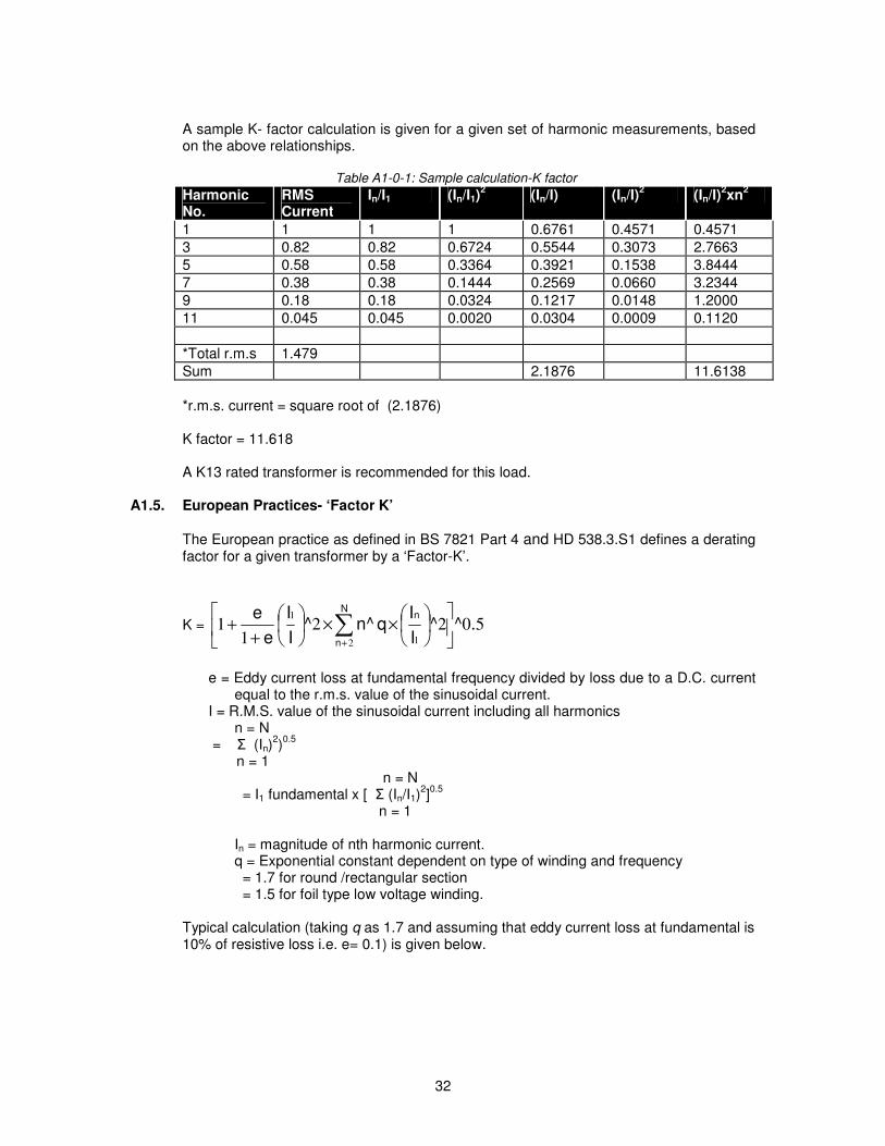
A sample K- factor calculation is given for a given set of harmonic measurements, based on the above relationships.

Table A1-0-1: Sample calculation-K factor

Harmonic No.

RMS Current

In/I1 (In/I1)2 (In/I) (In/I)

2 (In/I)

2xn

2

1 1 1 1 0.6761 0.4571 0.4571

3 0.82 0.82 0.6724 0.5544 0.3073 2.7663

5 0.58 0.58 0.3364 0.3921 0.1538 3.8444

7 0.38 0.38 0.1444 0.2569 0.0660 3.2344

9 0.18 0.18 0.0324 0.1217 0.0148 1.2000

11 0.045 0.045 0.0020 0.0304 0.0009 0.1120

*Total r.m.s 1.479

Sum 2.1876 11.6138

*r.m.s. current = square root of (2.1876) K factor = 11.618 A K13 rated transformer is recommended for this load.

A1.5. European Practices- ‘Factor K’ The European practice as defined in BS 7821 Part 4 and HD 538.3.S1 defines a derating factor for a given transformer by a ‘Factor-K’.

K = 50221

12 1

1

.^^I

Iq^n^

I

I

e

e N

n

n

××

++ ∑

+

e = Eddy current loss at fundamental frequency divided by loss due to a D.C. current

equal to the r.m.s. value of the sinusoidal current. I = R.M.S. value of the sinusoidal current including all harmonics

n = N = Σ (In)

2)0.5

n = 1

n = N = I1 fundamental x [ Σ (In/I1)

2]0.5

n = 1 In = magnitude of nth harmonic current. q = Exponential constant dependent on type of winding and frequency = 1.7 for round /rectangular section = 1.5 for foil type low voltage winding.

Typical calculation (taking q as 1.7 and assuming that eddy current loss at fundamental is 10% of resistive loss i.e. e= 0.1) is given below.

33

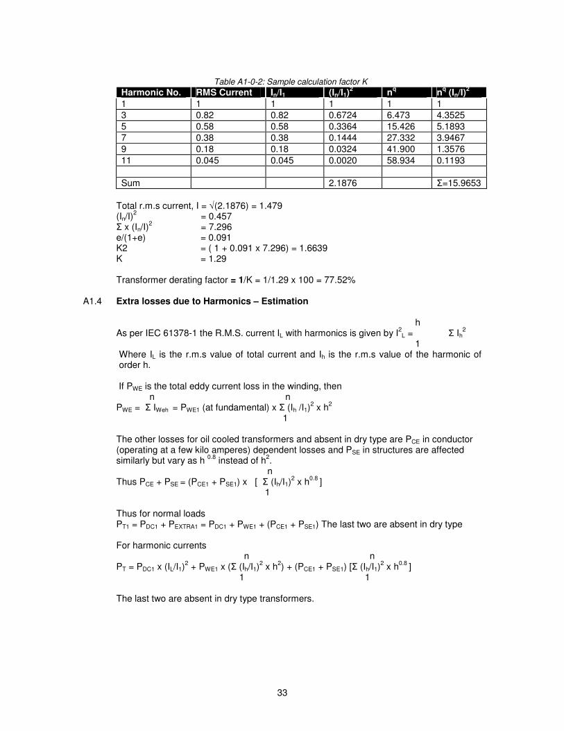
Table A1-0-2: Sample calculation factor K

Harmonic No. RMS Current In/I1 (In/I1)2 n

q n

q (In/I)

2

1 1 1 1 1 1

3 0.82 0.82 0.6724 6.473 4.3525

5 0.58 0.58 0.3364 15.426 5.1893

7 0.38 0.38 0.1444 27.332 3.9467

9 0.18 0.18 0.0324 41.900 1.3576

11 0.045 0.045 0.0020 58.934 0.1193

Sum 2.1876 Σ=15.9653

Total r.m.s current, I = √(2.1876) = 1.479 (In/I)

2 = 0.457

Σ x (In/I)2 = 7.296

e/(1+e) = 0.091 K2 = ( 1 + 0.091 x 7.296) = 1.6639 K = 1.29 Transformer derating factor = 1/K = 1/1.29 x 100 = 77.52% A1.4 Extra losses due to Harmonics – Estimation h

As per IEC 61378-1 the R.M.S. current IL with harmonics is given by I2L = Σ Ih

2

1 Where IL is the r.m.s value of total current and Ih is the r.m.s value of the harmonic of order h.

If PWE is the total eddy current loss in the winding, then n n PWE = Σ IWeh = PWE1 (at fundamental) x Σ (Ih /I1)

2 x h

2

1 The other losses for oil cooled transformers and absent in dry type are PCE in conductor (operating at a few kilo amperes) dependent losses and PSE in structures are affected similarly but vary as h

0.8 instead of h

2.

n Thus PCE + PSE = (PCE1 + PSE1) x [ Σ (Ih/I1)

2 x h

0.8 ]

1 Thus for normal loads PT1 = PDC1 + PEXTRA1 = PDC1 + PWE1 + (PCE1 + PSE1) The last two are absent in dry type For harmonic currents n n PT = PDC1 x (IL/I1)

2 + PWE1 x (Σ (Ih/I1)

2 x h

2) + (PCE1 + PSE1) [Σ (Ih/I1)

2 x h

0.8 ]

1 1 The last two are absent in dry type transformers.

34

ANNEXURE-2: REFERENCES

1. IS 2026- 1977– Specifications for Power Transformers 2. IEEE Standard C57.12.90 – 1993: IEEE Standard Test Code for Dry Type Distribution

Transformers 3. Energy Saving In Industrial Distribution Transformers- W.T.J. Hulshorst, J.F. Groeman,

KEMA 4. Discussion on Transformer testing in the factory- William R. Herron III, ABB Power T&D

Company Inc. 5. Harmonics, Transformers & K factors – Copper development Association – Publication

144