bayesian computational techniques for inverse …
TRANSCRIPT

BAYESIAN COMPUTATIONAL TECHNIQUES FOR INVERSE
PROBLEMS IN TRANSPORT PROCESSES
A Dissertation
Presented to the Faculty of the Graduate School
of Cornell University
in Partial Fulfillment of the Requirements for the Degree of
Doctor of Philosophy
by
Jingbo Wang
January 2006

c© Jingbo Wang 2006
ALL RIGHTS RESERVED
BAYESIAN COMPUTATIONAL TECHNIQUES FOR INVERSE PROBLEMS
IN TRANSPORT PROCESSES
Jingbo Wang, Ph.D.
Cornell University 2006
Inverse problems in continuum transport processes (governed by partial dif-
ferential equations (PDEs)) have major applications in a variety of scientific and
engineering areas. The ill-posedness, high computational cost, and other compli-
cations of these problems pose significant intellectual challenges. In this thesis, a
computational framework is developed that integrates computational mathematics,
Bayesian statistics, statistical computation, and reduced-order modeling to address
data-driven inverse heat and mass transfer problems. The Bayesian computational
approach is advantageous in many aspects. In particular, it is able to quantify
system uncertainty and random data error, to derive a probabilistic description of
the inverse solution, to provide flexible spatial/temporal regularization to the ill-
posedness of the inverse problem, and to allow adaptive sequential estimation. The
components of this framework include hierarchical Bayesian formulation, prior mod-
eling of distributed parameters via spatial statistics, exploration of implicit posterior
distributions using Markov chain Monte Carlo (MCMC) simulation, proper orthog-
onal decomposition (POD)-based reduced-order modeling of the PDE system, and
sequential Bayesian estimation. These methodologies are applied to the solution of

a number of inverse problems in transport processes including inverse heat conduc-
tion, inverse heat radiation, contaminant detection in porous media flows, control of
directional solidification, and multiscale permeability estimation in heterogeneous
media. These problems are selected due to their technological significance as well as
their ability to demonstrate the attributes of the Bayesian computational approach.
The developed methodologies are general and applicable to many other inverse con-
tinuum problems. A summary of achievements and suggestions for future research
are given at the end of the thesis.

Biographical Sketch
The author was born in Shaanxi, China in February, 1978. After completing his
high school education from Bao Shi High School in Baoji, China, the author was
admitted into Mechanical Engineering program at Tsinghua University, Beijing in
1996, from where he received his Bachelor’s degree in engineering in June, 2000.
In August, 2000, the author was admitted into the graduate school at University
of Delaware, and awarded a Master of Science degree in July, 2002. The author
entered the doctoral program at the Sibley School of Mechanical and Aerospace
Engineering, Cornell University in August, 2002.
iii

This thesis is in memory of my father Wang, Fulin. The thesis is also dedicated to
my mother Wang, Xiaoping and my sister Wang, Jingyuan for their constant
support and encouragement towards academic pursuits during my school years.
iv

Acknowledgements
I would like to thank my thesis advisor, Professor Nicholas Zabaras, for his constant
support and guidance over the last 3 years. I would also like to thank Professors
David Ruppert and Thorsten Joachims for serving on my special committee and
for their encouragement and suggestions at various times during the course of this
work.
The financial support for this project was provided by NASA (grant NAG8-
1671) and the National Science Foundation (grant DMI-0113295). Partial support
from the Advanced Mechanical Technologies Program at General Electric Global
Research Center (GE-GRC) is also gratefully acknowledged. I would like to thank
the Sibley School of Mechanical and Aerospace Engineering for having supported
me through a teaching assistantship for part of my study at Cornell. The computing
for this project was supported by the Cornell Theory Center during 2002-2005.
Part of the computer codes associated with this project were written using the
object oriented programming environment of Diffpack and the academic license
that allowed for these developments is appreciated. The parallel simulators were
developed based on open source scientific computation package Pestc. I would
like to acknowledge the effort of its developers. I am indebted to the present and
former members of the MPDC group, especially to Shankar Ganapathysubramanian,
v

Baskar Ganapathysubramanian and Lijian Tan. Finally, my thanks are extended
to the Elsevier, Ltd. and Institute of Physics and IOP Publishing Ltd. for granting
permission to reproduce figures from our papers [29, 32, 31, 30].
vi

Table of Contents
Table of Contents vii
List of Tables x
List of Figures xi
1 Introduction 1
2 Fundamentals of Bayesian computation and Markov Random Field(MRF) 112.1 Bayesian statistical analysis . . . . . . . . . . . . . . . . . . . . . . . 112.2 Markov chain Monte Carlo (MCMC) simulation . . . . . . . . . . . . 15
2.2.1 Monte Carlo principle . . . . . . . . . . . . . . . . . . . . . . 152.2.2 MCMC algorithms . . . . . . . . . . . . . . . . . . . . . . . . 162.2.3 Convergence assessment of MCMC . . . . . . . . . . . . . . . 19
2.3 Prior distribution modeling using MRF . . . . . . . . . . . . . . . . . 192.4 Generic Bayesian computational framework for inverse continuum
problems . . . . . . . . . . . . . . . . . . . . . . . . . . . . . . . . . . 21
3 Inverse heat conduction problems (IHCP) - A Bayesian approach 223.1 The inverse heat conduction problems . . . . . . . . . . . . . . . . . . 233.2 Bayesian formulation of the inverse heat conduction problems . . . . 26
3.2.1 The likelihood . . . . . . . . . . . . . . . . . . . . . . . . . . . 273.2.2 Prior distribution modeling . . . . . . . . . . . . . . . . . . . 273.2.3 The posterior distributions . . . . . . . . . . . . . . . . . . . . 303.2.4 Regularization in the Bayesian approach . . . . . . . . . . . . 32
3.3 Parameter estimation . . . . . . . . . . . . . . . . . . . . . . . . . . . 343.4 Heat flux reconstruction under uncertainties . . . . . . . . . . . . . . 37
3.4.1 Automatic selection of the regularization parameter . . . . . . 373.4.2 Effect of the sensor location . . . . . . . . . . . . . . . . . . . 403.4.3 IHCP under model uncertainties . . . . . . . . . . . . . . . . . 41
3.5 Examples . . . . . . . . . . . . . . . . . . . . . . . . . . . . . . . . . 433.5.1 Example I: Parameter estimation . . . . . . . . . . . . . . . . 43
vii

3.5.2 Example II: Boundary heat flux estimation . . . . . . . . . . . 463.5.3 Example III: Boundary heat flux identification with simul-
taneous uncertainties in material property and thermocouplelocation . . . . . . . . . . . . . . . . . . . . . . . . . . . . . . 50
3.5.4 Example IV: 1D piece-wise continuous heat source identification 523.5.5 Example V: 2D heat source identification . . . . . . . . . . . . 54
3.6 Summary . . . . . . . . . . . . . . . . . . . . . . . . . . . . . . . . . 57
4 Inverse heat radiation problem (IHRP)- An integrated reduced-order modeling and Bayesian computational approach to complexinverse continuum problems 584.1 The inverse heat radiation problem (IHRP) . . . . . . . . . . . . . . . 594.2 Direct simulation and reduced-order modeling . . . . . . . . . . . . . 624.3 Bayesian formulation of IHRP . . . . . . . . . . . . . . . . . . . . . . 674.4 MCMC sampler . . . . . . . . . . . . . . . . . . . . . . . . . . . . . . 694.5 Numerical examples . . . . . . . . . . . . . . . . . . . . . . . . . . . . 704.6 Summary . . . . . . . . . . . . . . . . . . . . . . . . . . . . . . . . . 82
5 Contamination source identification in porous media flow - Solvingthe PDEs backward in time using Bayesian method 835.1 Problem definition . . . . . . . . . . . . . . . . . . . . . . . . . . . . 845.2 The direct simulation and sensitivity analysis . . . . . . . . . . . . . 87
5.2.1 Solution of the flow equations . . . . . . . . . . . . . . . . . . 875.2.2 Solution of the concentration equation . . . . . . . . . . . . . 885.2.3 Sensitivity analysis . . . . . . . . . . . . . . . . . . . . . . . . 89
5.3 Bayesian backward computation . . . . . . . . . . . . . . . . . . . . . 915.3.1 Bayesian inverse formulation . . . . . . . . . . . . . . . . . . . 915.3.2 The hierarchical posterior distribution . . . . . . . . . . . . . 925.3.3 The backward marching scheme . . . . . . . . . . . . . . . . . 93
5.4 Numerical exploration of the posterior distribution . . . . . . . . . . 945.5 Numerical examples . . . . . . . . . . . . . . . . . . . . . . . . . . . . 96
5.5.1 Example 1: 1D advection-dispersion in homogeneous media . . 965.5.2 Example 2: 2D concentration reconstruction . . . . . . . . . . 98
5.6 Summary . . . . . . . . . . . . . . . . . . . . . . . . . . . . . . . . . 106
6 Open-loop control of directional solidification - A sequential Bayesiancomputational application 1086.1 Open-loop control of directional solidification using magnetic gradient 1106.2 A Bayesian filter-based control approach . . . . . . . . . . . . . . . . 114
6.2.1 Bayesian filter . . . . . . . . . . . . . . . . . . . . . . . . . . . 1146.2.2 A sequential Bayesian controller for solidification control . . . 116
6.3 Examples . . . . . . . . . . . . . . . . . . . . . . . . . . . . . . . . . 1206.4 Summary . . . . . . . . . . . . . . . . . . . . . . . . . . . . . . . . . 131
viii

7 Multiscale permeability estimation in heterogeneous porous media- A multiscale Bayesian inversion method 1327.1 Problem definition . . . . . . . . . . . . . . . . . . . . . . . . . . . . 1337.2 Bayesian posterior distribution of the random permeability . . . . . . 135
7.2.1 Formulation I: MRF-based one scale model . . . . . . . . . . . 1367.2.2 Formulation II: HMT-based two scale model . . . . . . . . . . 1377.2.3 Exploring the posterior state space . . . . . . . . . . . . . . . 142
7.3 Examples . . . . . . . . . . . . . . . . . . . . . . . . . . . . . . . . . 1477.3.1 Example I - permeability with bilinear logarithm . . . . . . . 1477.3.2 Example II - permeability of a random heterogeneous medium 149
7.4 Summary . . . . . . . . . . . . . . . . . . . . . . . . . . . . . . . . . 153
8 Conclusions and suggestions for the future research 1558.1 Pattern recognition for reduced-order modeling . . . . . . . . . . . . 1578.2 Enhancing the multiscale Bayesian inversion techniques . . . . . . . . 1588.3 Wavelet function representation . . . . . . . . . . . . . . . . . . . . . 159
Bibliography 161
ix

List of Tables
3.1 Bayesian estimates of k using different models. . . . . . . . . . . . . 44
6.1 Specifications of the direct solidification problem. . . . . . . . . . . . 120
x

List of Figures
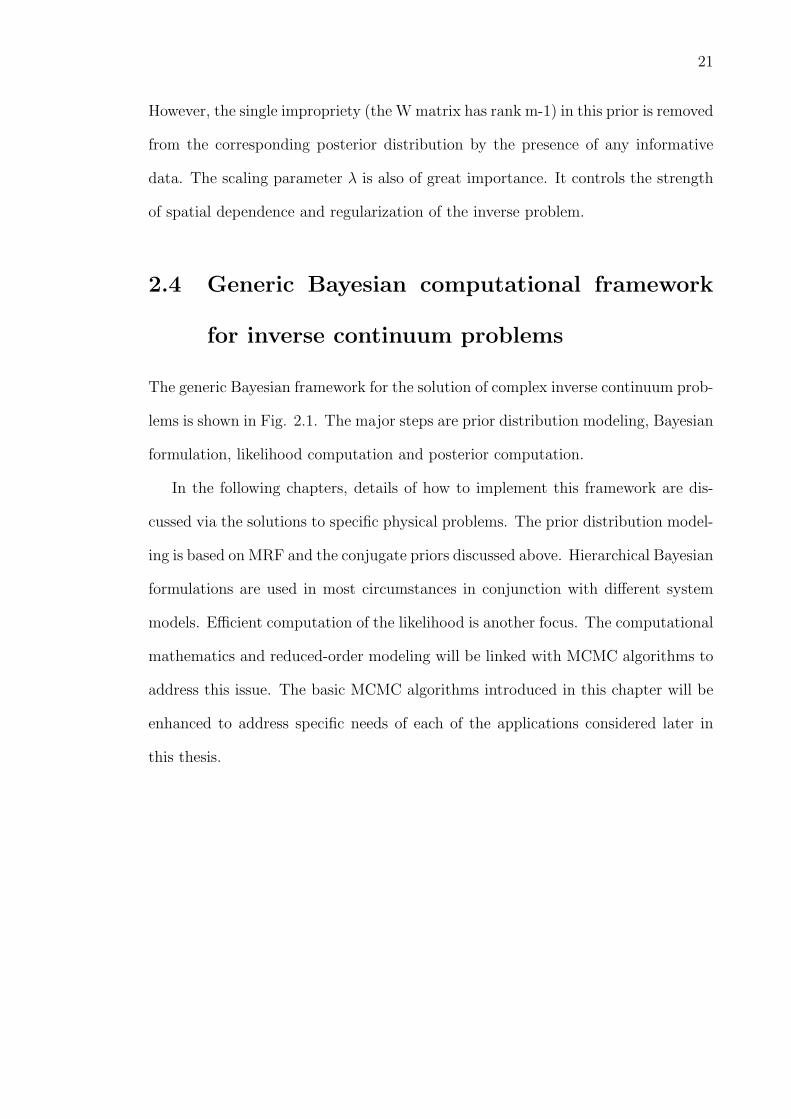
2.1 Schematic of Bayesian computation for inverse continuum problems. 20
3.1 Schematic for inverse problems in heat conduction. The main un-knowns considered include the conductivity k, the heat flux q0 on Γ0
or the heat source f(x, t) in Ω. . . . . . . . . . . . . . . . . . . . . . 243.2 Linear finite element basis functions and neighborhood definition for
θ. The figure on the left refers to 1D heat conduction (unknownheat flux q(t)) and the figure on the right to 2D heat conduction ina square domain (unknown heat flux shown q(x, t)). . . . . . . . . . 29
3.3 The left figure is the schematic of the 1D inverse heat conductionproblem. The figure on the right provides the time-profile of thetrue heat flux that was used to generate the simulated sensor data. . 43
3.4 Computed posterior densities of k using different Bayesian models. . 453.5 True heat flux in example II. . . . . . . . . . . . . . . . . . . . . . . 463.6 Posterior mean estimates of the heat flux and 98% probability bounds
of the posterior distributions when d = 0.5 using a hierarchicalBayesian model (Example II). The figure on the left is obtained whenσT = 0.01 and the figure on the right is obtained when σT = 0.001. . 47
3.7 Posterior mean estimates of the heat flux and 98% probability boundsof the posterior distributions when d = 0.1 using a hierarchicalBayesian model (Example II). The figure on the left is obtained whenσT = 0.01 and the figure on the right is obtained when σT = 0.001. . 48
3.8 Posterior mean estimates of the heat flux and 98% probability boundsof the posterior distribution when d = 0.5 and σT = 0.01 using a hi-erarchical and augmented Bayesian model (Example II). . . . . . . . 49
3.9 Posterior density estimate of hyper-parameter λ in the second case. . 493.10 Posterior mean estimates of the heat flux and 98% probability bounds
of the posterior distribution when uncertainties in d and k exist. Thefigure on the left is obtained using true d and k, and the figure onthe right is obtained using the nominal values of d and k (ExampleIII). . . . . . . . . . . . . . . . . . . . . . . . . . . . . . . . . . . . . 50
3.11 Posterior mean estimates of the heat flux and 98% probability boundsof the posterior distribution when k and d are treated as randomvariables (Example III). . . . . . . . . . . . . . . . . . . . . . . . . . 51
xi

3.12 True heat source (left) and reconstructed heat source (right) for caseII of Example IV. . . . . . . . . . . . . . . . . . . . . . . . . . . . . 53
3.13 Posterior mean estimate and 98% probability bounds of the posteriordistribution of step heat source at t = 0.24. . . . . . . . . . . . . . . 53
3.14 True heat source profiles for example V. . . . . . . . . . . . . . . . . 543.15 Posterior mean estimates of heat source profiles when σT = 0.02 for
example V. . . . . . . . . . . . . . . . . . . . . . . . . . . . . . . . . 553.16 Computed heat source at y = 0.725 at different times (example V,
σT = 0.005). Also shown are the 98% probability bounds of theposterior distribution at t = 0.05. . . . . . . . . . . . . . . . . . . . . 56
4.1 Schematic of the inverse radiation problem. The objective is to com-pute the point heat source g(t) given initial conditions, boundaryconditions on the surface and temperature measurements at a num-ber of points within the domain. . . . . . . . . . . . . . . . . . . . . 61
4.2 Schematic of the numerical example. . . . . . . . . . . . . . . . . . . 714.3 Profile of the step heat source. . . . . . . . . . . . . . . . . . . . . . 714.4 Homogeneous intensity fields on y = 0.5 along directions [0.9082
483 0.2958759 0.2958759] and [−0.90824830.29587590.2958759] for stepheat source. . . . . . . . . . . . . . . . . . . . . . . . . . . . . . . . . 73
4.5 Homogeneous temperature fields on y = 0.5 for step heat source. . . 744.6 Eigenfunctions of Ih along [0.9082483 0.2958759 0.2958759] on y = 0.5. . 754.7 Eigenfunctions of T h on y = 0.5. . . . . . . . . . . . . . . . . . . . . 764.8 Homogeneous temperature field computed using the POD method
on y = 0.5 for step heat source. . . . . . . . . . . . . . . . . . . . . . 774.9 Temperature evolution at thermocouple locations for step heat source. 784.10 MAP estimates for the step heat source. . . . . . . . . . . . . . . . . 794.11 Posterior mean estimate of the step heat source and probability
bounds of the posterior distribution when σT = 0.01. . . . . . . . . . 804.12 Profile of the triangular heat source. . . . . . . . . . . . . . . . . . . 804.13 MAP estimates for the triangular heat source case. . . . . . . . . . . 814.14 Posterior mean estimate of the triangular heat source and probability
bounds of the posterior distribution when σ = 0.01. . . . . . . . . . . 81
5.1 True and posterior mean estimate of concentration at t = 1.1. . . . . 975.2 True and posterior mean estimate of concentration at t = 1.9. . . . . 975.3 Posterior density of structure parameter λ in obtaining concentration
estimate at t = 1.1. . . . . . . . . . . . . . . . . . . . . . . . . . . . . 985.4 Schematic of Example 2. . . . . . . . . . . . . . . . . . . . . . . . . . 995.5 Reconstruction of the history of contaminant concentration: (a) The
true concentrations at different past time steps; (b) the reconstructedconcentrations. . . . . . . . . . . . . . . . . . . . . . . . . . . . . . . 100
xii

5.6 Reconstruction of the concentration at t = 0: (a) data are collectedat 9 × 9 sensor locations at t = 0.2 (b) data are collected at 5 × 5sensor locations at t = 1.0. . . . . . . . . . . . . . . . . . . . . . . . 101
5.7 Reconstruction of the history of pollute concentration: (a) showsthe true concentrations at different past time steps and (b) showsthe reconstructions. . . . . . . . . . . . . . . . . . . . . . . . . . . . 103
5.8 Reconstruction of the contamination history when data are collectedat 9× 9 sensor locations at t = 1.0. . . . . . . . . . . . . . . . . . . . 104
5.9 Reconstruction of the history of pollute concentration in heteroge-neous medium (data are collected at 32 × 32 grid): (a) the trueconcentrations at different past time steps and (b) the computedreconstructions. . . . . . . . . . . . . . . . . . . . . . . . . . . . . . . 105
5.10 Reconstruction of the history of pollute concentration in heteroge-neous medium (data are collected on a 16× 16 grid). . . . . . . . . . 106
6.1 Schematic of the directional solidification system. A time-varying
magnetic field with spatial gradient ∂B∂z
is applied in the z direction. 1126.2 Schematic of a Bayesian filter with Markov properties. . . . . . . . . 1156.3 Snapshots of the solidification process without magnetic gradient
control applied. The left figures are the temperature fields and theright ones are the streamlines. . . . . . . . . . . . . . . . . . . . . . . 121
6.4 Configuration of the optimal magnetic gradient when λ = 0.1. . . . . 1216.5 Configuration of the optimal magnetic gradient when λ = 0.5. . . . . 1226.6 Configuration of the optimal magnetic gradient when λ = 1. . . . . . 1226.7 Snapshots of the solidification process with optimal magnetic gradi-
ent applied when λ = 0.1. The left figures are the temperature fieldsand the right ones are the streamlines. . . . . . . . . . . . . . . . . . 124
6.8 Snapshots of the solidification process with optimal magnetic gradi-ent applied when λ = 0.5. The left figures are the temperature fieldsand the right ones are the streamlines. . . . . . . . . . . . . . . . . . 125
6.9 Snapshots of the solidification process with optimal magnetic gradi-ent applied when λ = 1. The left figures are the temperature fieldsand the right ones are the streamlines. . . . . . . . . . . . . . . . . . 126
6.10 Configuration of the optimal magnetic gradient when the boundaryheat flux has random fluctuation with a uniform distribution. . . . . 127
6.11 Configuration of the optimal magnetic gradient when the boundaryheat flux has random fluctuation with a Gaussian distribution. . . . 127
6.12 Snapshots of the solidification process with optimal magnetic gra-dient applied when the boundary heat flux has random fluctuationwith a uniform distribution. The left figures are the temperaturefields and the right ones are the streamlines. . . . . . . . . . . . . . . 128
xiii

6.13 Snapshots of the solidification process with optimal magnetic gra-dient applied when the boundary heat flux has random fluctuationwith a Gaussian distribution. The left figures are the temperaturefields and the right ones are the streamlines. . . . . . . . . . . . . . . 129
7.1 Schematic of a 9-spot problem. A injection well is located at thecenter of the domain and 8 production wells distribute at the restnodes of a 2 × 2 grid. In general, for a n-spot problem, the n wellsdistribute at nodes of a (
√n − 1) × (
√n − 1) grid with the single
injection well at the center. . . . . . . . . . . . . . . . . . . . . . . . 1347.2 The log permeability of a random porous medium. Two large mag-
nitude discontinuities occur within two darker areas ([2, 4] × [4, 6]and [4, 6] × [2, 4]). Within each of these areas, the permeability isa correlated Gaussian random field with a correlation function ofρ(r) = e−r2
with r being the spatial distance among two locations.The random variations within each darker area have much smallermagnitude than the average magnitudes of both darker areas perme-ability. . . . . . . . . . . . . . . . . . . . . . . . . . . . . . . . . . . . 138
7.3 The enlarged upper-left darker area ([2, 4]× [4, 6]) of the log perme-ability in Fig. 7.2. . . . . . . . . . . . . . . . . . . . . . . . . . . . . 138
7.4 The enlarged lower-right darker area ([4, 6]×[2, 4]) of log permeabilityin Fig. 7.2. . . . . . . . . . . . . . . . . . . . . . . . . . . . . . . . . 139
7.5 A scheme of hierarchical Markov tree model. . . . . . . . . . . . . . . . 1407.6 Schematics of single component updating (upper-left), block updat-
ing (upper-right), and whole field updating (lower). . . . . . . . . . . 1437.7 The true permeability field in example I. . . . . . . . . . . . . . . . . 1457.8 The permeability estimate on 32× 32 grid using data at 24 wells. . . 1457.9 The permeability estimate on 16× 16 grid using data at 24 wells. . . 1467.10 The permeability estimate on 8× 8 resolution using data at 24 wells. 1467.11 The permeability estimate on 32×32 resolution using data at 8 wells
without smoothing. . . . . . . . . . . . . . . . . . . . . . . . . . . . 1477.12 The permeability estimate on 32×32 resolution using data at 8 wells
with smoothing. . . . . . . . . . . . . . . . . . . . . . . . . . . . . . 1487.13 The permeability estimate on 16×16 resolution using data at 8 wells
with smoothing. . . . . . . . . . . . . . . . . . . . . . . . . . . . . . 1487.14 The permeability estimate on 8× 8 resolution using data at 8 wells
with smoothing. . . . . . . . . . . . . . . . . . . . . . . . . . . . . . 1497.15 The coarse scale estimate of the random heterogeneous permeability
(logarithm of the permeability is plotted). . . . . . . . . . . . . . . . 1507.16 Realization I of the fine scale log permeability distribution. The left
plot is the entire field. The middle plot is the enlarged upper-leftdarker area ([2, 4]× [4, 6]). The right plot is the enlarged lower-rightdarker area ([4, 6]× [2, 4]). . . . . . . . . . . . . . . . . . . . . . . . . 150
xiv

7.17 Realization II of the fine scale log permeability distribution. The leftplot is the entire field. The middle plot is the enlarged upper-leftdarker area ([2, 4]× [4, 6]). The right plot is the enlarged lower-rightdarker area ([4, 6]× [2, 4]). . . . . . . . . . . . . . . . . . . . . . . . . 151
7.18 Realization III of the fine scale log permeability distribution. Theleft plot is the entire field. The middle plot is the enlarged upper-leftdarker area ([2, 4]× [4, 6]). The right plot is the enlarged lower-rightdarker area ([4, 6]× [2, 4]). . . . . . . . . . . . . . . . . . . . . . . . . 151
7.19 Sample mean of the fine scale log permeability distribution. The leftplot is the entire field. The middle plot is the enlarged upper-leftdarker area ([2, 4]× [4, 6]). The right plot is the enlarged lower-rightdarker area ([4, 6]× [2, 4]). . . . . . . . . . . . . . . . . . . . . . . . . 152
7.20 True log permeability with correlation coefficient ρ = e−|r|. The leftplot is the entire field. The middle plot is the enlarged upper-leftdarker area ([2, 4]× [4, 6]). The right plot is the enlarged lower-rightdarker area ([4, 6]× [2, 4]). . . . . . . . . . . . . . . . . . . . . . . . . 153
7.21 Realization I of the fine scale log permeability distribution with ρ =e−|r|. The left plot is the entire field. The middle plot is the enlargedupper-left darker area ([2, 4]× [4, 6]). The right plot is the enlargedlower-right darker area ([4, 6]× [2, 4]). . . . . . . . . . . . . . . . . . 153
7.22 Realization II of the fine scale log permeability distribution withρ = e−|r|. The left plot is the entire field. The middle plot is theenlarged upper-left darker area ([2, 4]× [4, 6]). The right plot is theenlarged lower-right darker area ([4, 6]× [2, 4]). . . . . . . . . . . . . 154
xv

Chapter 1
Introduction
Continuum systems herein refer to physical systems described by partial differential
equations (PDEs). The direct or forward problem in continuum systems (direct
continuum problem) computes the solution to the PDEs with complete specifica-
tion of all pertinent physical information including spatial and temporal domains,
boundary conditions, initial conditions, as well as other physical parameters. To
the contrary, the inverse problem in continuum systems (inverse continuum prob-
lem) concerns determination of unknown boundary conditions, initial conditions,
physical parameters or geometry from known information about the governing con-
tinuum fields. This known information usually takes the form of discrete values of
these fields (experimental data or desired system response) at given spatial and tem-
poral locations. Thus the majority of inverse problems are data-driven in nature.
Inverse continuum problems are generally stochastic, e.g. random errors are always
present in experimentally collected data.
Inverse continuum problems have major applications in almost all scientific and
engineering areas. For example, among the physical problems studied in this the-
sis, inverse heat conduction is of interest in broad areas including manufacturing
1

2
process control; metallurgy; chemical, aerospace and nuclear engineering; food sci-
ence; medical diagnostics; etc. [1]. In this problem, one seeks the heat flux along
part of the boundary of a domain given sufficient conditions along the remaining
part of the boundary and temperature measurements within the domain of a con-
ducting solid. Another example is the study of inverse thermal radiation, in which
the heat source is determined from temperature data. This problem is motivated
by thermal control applications in space technology, combustion, high temperature
forming and coating technology, solar energy utilization, high temperature engine,
furnace technology and other areas [2]. Inverse continuum problems are very com-
mon in many mass transport processes such as detection of a contaminant source
in groundwater, estimation of heterogeneous permeability of subsurface structures,
identification of species generation rates in chemical reactions, identification of in-
jection rates or initial concentrations in miscible/immiscible displacements of fluids
in porous media, etc. In addition, design and many open-loop control problems in
continuum systems can be posed as inverse problems by treating design or control
objectives as measured data.
Inverse continuum problems have received enormous research interest because of
their technological significance and their mathematical and computational difficul-
ties. The main characteristic of an inverse continuum problem versus a well-posed
direct continuum problem is that it leads to solutions that generally are not unique or
stable to small changes in the given data [3], and this characteristic is often referred
to as ill-posedness. Additional features of solution procedures for solving inverse
continuum problems include the complexity of the direct simulation and the result-
ing implicit inverse formulation, the high computational cost, and the existence of
various uncertainties. The inverse problem requires solution of the direct continuum

3
process specified by a coupled system of PDEs. Discontinuities and singularities are
often expected in the unknowns as in the case of estimating heterogeneous random
fields in porous media. For a complex continuum transport system, the degrees-
of-freedom (DOF) of the numerical simulation can easily reach the hundreds of
thousands, millions or higher. Uncertainties are also unavoidable and have critical
effects on the inverse solutions. They arise, for example, from instability of the
physics, from insufficient knowledge of the underlying physical and mathematical
models, from lack of knowledge of material properties and initial/boundary condi-
tions, from propagation of errors in the simulation and of course from noise-polluted
experimental data. These features are summarized in Box 1.
• ill-posedness (non-unique solution and instability
to random error)
• complexity of direct simulation
• non-linearity and complex objective function re-
sponse surface
• high computational cost
• discontinuity in the distributed unknown fields
• system and measurement uncertainties
• sparseness of the data
Box 1: Features of inverse continuum problems
Many methods have been developed for the solution of inverse continuum prob-
lems with the majority of them restating the problem as a least-squares minimization
problem [4, 5, 6] (or using other appropriate norms of the deviation between the com-
puted PDE variables at the sensor locations for a guessed inverse solution and the

4
given measured data). The inverse problem is formulated using either a parametric
approach, where the unknown is first discretized using specified basis functions and
the coefficients are then estimated, or using an infinite-dimension functional opti-
mization approach, in which the functional form of the unknown is not prescribed
[7]. In addition to the direct problem, appropriate continuum or discrete sensitivity
and/or adjoint problems are usually required [8, 9]. The ill-posedness of the inverse
problem is addressed using the Tikhonov regularization technique [10, 11, 12], the
future information method [1, 13], the iterative regularization technique [3, 14], or
the mollification method [15]. The optimization problem is usually solved via a gra-
dient method such as the conjugate gradient method in either a finite or an infinite
dimensional space.
The above deterministic inverse techniques lead to point estimates of unknowns
without rigorously considering the statistical nature of system uncertainties and
without providing quantification of the uncertainty in the inverse solution. For many
inverse problems, these methods do not provide satisfactory solutions. The existing
regularization methods smooth the inverse solution without resolving its disconti-
nuities. Such techniques omit two types of useful information in regularizing the
ill-posed inverse problems: the accumulated prior knowledge of the unknowns and
the spatial and temporal dependence among the unknowns. The drawbacks restrict
their ability to solve distributed parameter estimation problems. Also, the selection
of an optimal regularization parameter is a problem common to all regularization
methods. Furthermore, the gradient method used in minimizing the deterministic
optimization objective often fails to locate the global minimum for highly nonlinear
problems. Finally, since the existing inverse methods do not consider prior informa-
tion regarding the unknowns besides measured data, obtaining a valid solution to

5
the inverse problem becomes less feasible when only sparse data are available.
• models uncertainties probabilistically and determines their propagation
through the inverse solution
• solves the direct problem deterministically with reduced-order models
• transforms the inverse problem into a well-posed problem in an expanded
stochastic space
• explores state space of the regularization parameter and allows selection
of its optimal value
• links with spatial statistics models for prior distribution modeling
• obtains accurate estimates using sparse data through prior distribution
modeling
• enables computation of statistics of inverse solution
Box 2: Advantages of the Bayesian computational approach
With the rapid growth of computational power and critical demands on robust-
ness and reliability, solving inverse problems under uncertainty has become more and
more important. Lately a number of methods have been proposed to solve stochastic
inverse problems, including the sensitivity analysis [16, 17], the extended maximum
likelihood estimator (MLE) approach [18, 19], the spectral stochastic method [20],
and the Bayesian inference method [21, 22, 23]. While all stochastic inverse meth-
ods can account for uncertainties and are able to provide point estimates to the
inverse solution with credible intervals, the Bayesian approach has more assets. In
the Bayesian approach, a prior distribution model is combined with the likelihood to
formulate the posterior probability density function (PPDF) of the unknown vari-
able [24, 25]. The Bayesian approach provides a complete probabilistic description

6
of the unknown quantities given all related observations. The method regularizes
the ill-posed inverse problem through prior distribution modeling [21] and in addi-
tion provides means to estimate the statistics of uncertainties. The advantages of
the Bayesian approach are summarized in Box 2.
The Bayesian approach can probabilistically model various system uncertainties
and determine their propagation to the inverse solution [26]. Therefore, it provides
not only point estimates but also the probability distribution of the unknown quan-
tities conditional on available data [27]. The Bayesian method explores statistics of
random data error, which is rather critical because solutions to inverse problems are
extremely sensitive to data error [28]. In addition, unlike other techniques that aim
to regularize the ill-posed inverse problem to achieve a point estimate, the Bayesian
method treats the inverse problem as a well-posed problem in an expanded sto-
chastic space [27]. Even when seeking only a point estimate, the Bayesian method
can provide more flexible regularization to the inverse problem [29, 30] in the sense
that the non-trivial problem of selecting the regularization parameter [10] is solved
through hierarchical Bayesian formulations [31]. Furthermore, under the Bayesian
framework, the forward problems are solved deterministically and the uncertain-
ties are accounted for solely through statistical inference [31]. Hence, legacy scien-
tific computational methods that simulate continuum processes can be used jointly
with Bayesian computational algorithms. Bayesian regularization through prior dis-
tribution modeling can deal with arbitrary unknown fields using spatial statistics
models [33, 34, 35]. It can provide accurate estimates with a limited number of mea-
surements when reliable prior models are available [36, 37]. Finally, the available
sampling strategies [38, 39] associated with Bayesian computation, especially the
Markov chain Monte Carlo (MCMC) simulation tools [40, 41, 42, 43, 44], are capa-

7
ble of overcoming the difficulties encountered when dealing with the optimization
of nonlinear problems of high-dimensionality.
Despite the rather long history of Bayesian statistics and development within
the past several decades of the computational method MCMC simulation, there are
few applications of Bayesian statistics to engineering inverse problems. The related
previous work includes those of Beck et al. [45] to structural models, of Kaipio et al.
[46] to electrical impedance tomography, of Sabin et al. [47] to grain size prediction,
of Michalak et al. [48] to flow in porous media, of Osio [49] to engineering design,
and of Higdon et al. [50] to petroleum engineering.
In this thesis, a computational framework that integrates computational math-
ematics aspects of PDEs, Bayesian statistics, statistical computation, as well as
reduced-order modeling is developed to address data-driven inverse problems in con-
tinuum systems. The components of this framework include hierarchical Bayesian
estimation, prior modeling of a distributed parameter via spatial statistics, explo-
ration of implicit posterior distribution using Markov chain Monte Carlo (MCMC)
simulation, proper orthogonal decomposition (POD) based reduced-order modeling
of PDE systems, as well as sequential Bayesian estimation. The emphasis in this the-
sis is on three aspects of inverse continuum problems: (i) developing methodologies
that enable probabilistic modeling and quantification of various uncertainties aris-
ing from physical instability, model and parameter insufficiency, and measurement
errors; (ii) computing inverse solutions with full-probabilistic specification; and (iii)
designing computational tools to address the high-computational cost in stochastic
optimization.
In the following chapters, presentation of the methodologies is fused with solu-
tions to physical problems including inverse heat conduction, inverse heat radiation,

8
contaminant detection in porous media flows, control of directional solidification,
and multiscale permeability estimation in heterogeneous media. The list of physical
problems is given in Box 3. These problems were selected due to their technical sig-
nificance as well as their ability to demonstrate the attributes of Bayesian method.
Among these problems, the inverse heat conduction problems, the inverse radia-
tion problem, and the solidification control problem have been studied by other
researchers. However, the Bayesian method improves the solutions to these prob-
lems in the following sense: i.) it quantifies the uncertainties in the inverse heat
conduction and radiation problems and provides statistics of the inverse solutions;
ii.) it allows estimates of discontinuous unknown heat source with sparse temper-
ature measurements; iii.) it saves computational time and memory cost for the
solidification control problem; and iv.) it enables an intelligent way to select the
regularization parameters in all of these problems. The problems of contaminant
detection in porous media flow (with heterogeneous permeability and anisotropic
dispersion) and the multiscale permeability estimation are unsolved problems (al-
though some related research was performed earlier as reviewed in the corresponding
chapters). It will be shown that the Bayesian method provides satisfactory solutions
to these problems.
The developed methodologies are generic and applicable to many other inverse
continuum problems. The new Bayesian computational approach provides a new
outlook to the solution of inverse continuum problems. This work will benefit a
variety of engineering and scientific areas such as materials and chemical process
monitoring/control, metallurgy, geology, combustion diagnostics, nuclear engineer-
ing, etc.

9
• inverse heat condition problems (IHCP)
• inverse heat radiation problem (IHRP)
• backward contamination source estimation problem (BCSEP)
• open-loop control of directional solidification using a non-
uniform external magnetic field
• multiscale permeability estimation in random heterogeneous
porous media
Box 3: Inverse problems of interest in this study
The outline of this thesis is as follows. In Chapter 2, the fundamental knowledge
of Bayesian computation pertaining to this study is reviewed, including Bayesian
statistics, MCMC and MRF. Chapter 3 elaborates the formulation of the posterior
probability density function (PPDF) for inverse heat conduction problems, includ-
ing boundary heat flux estimation, physical parameter estimation, and heat source
estimation. A sequence of MCMC samplers are designed for the posterior explo-
ration of IHCPs. In particular, hierarchical and augmented Bayesian models are
introduced for the purpose of automated regularization parameter selection as well
as uncertainty statistics estimation. Markov random fields (MRF) [51, 52] are used
to model the prior distributions of quantities varying in both space and time such as
heat flux and heat source. The objective of Chapter 3 is to demonstrate the funda-
mental steps in applying Bayesian computation to inverse continuum problems. In
Chapter 4, the Bayesian method is extended to a computationally expansive inverse
radiation problem. The focus of this Chapter is to fuse Bayesian inversion with
reduced-order modeling to address the high-computational cost associated with sto-
chastic inverse methods. In Chapter 5, Bayesian computation is further applied to

10
a backward inverse problem for estimation of contaminant source in porous media
flow. It demonstrates a backward marching in time procedure for addressing of
initial condition estimation problems. This is another type of inverse continuum
problems besides the boundary value estimation problems discussed in the previous
two chapters. Chapter 6 discusses a Bayesian filter approach for open-loop control
of directional solidification. This study accomplishes the Bayesian computational
framework by introducing sequential Bayesian estimation as complementary to the
whole-time domain method addressed in the previous chapters. It is aimed at illus-
trating a group of powerful sequential Bayesian computational methods that can be
applied to data-driven inversion in a dynamic continuum system. A multiscale in-
verse problem of estimating the permeability of heterogeneous porous medium using
flow data is finally presented in Chapter 7. The hierarchical Markov tree (HMT)
model is introduced to model random parameters at different length scales. The
conclusions of this work and suggestions for future research are finally summarized
in Chapter 8.

Chapter 2
Fundamentals of Bayesian
computation and Markov Random
Field (MRF)
This chapter provides information about Bayesian statistical analysis, the Markov
chain Monte Carlo (MCMC) computation method and Markov Random Field (MRF)
that are necessary background for the work presented in subsequent chapters. The
more advanced models and algorithms used to solve the actual problems in this thesis
are introduced in later chapters as the applications arise. For additional informa-
tion about these topics that is not covered in this thesis, readers are encouraged to
consult [24, 25, 26, 27].
2.1 Bayesian statistical analysis
Bayesian statistics study the probability of a hypothesis from both currently achieved
information (data) and previous knowledge (prior distribution) [26]. It provides
11

12
powerful analytical tools for parameter estimation, hypothesis testing, and model
selection problems, in particular those related to data-driven identification of input
parameters, satisfying robust design requirements, and real-time decision making.
The basis of Bayesian analysis is the Bayes’ formula:
p(θ|Y ) =p(Y |θ)p(θ)
p(Y )=
1
cp(Y |θ)p(θ). (2.1)
Here, θ is used to represent a hypothesis or a parameter and Y stands for the
observation (data) related to θ. p(θ|Y ), p(Y |θ) and p(θ) are the posterior probability
density function (PPDF), the likelihood and the prior probability density function,
respectively. Eq. (2.1) states that the posterior probability of a hypothesis given
some observations is proportional to the product of its likelihood and the prior
(unconditional) probability.
When θ represents a random parameter, the Bayes formula defines its distribu-
tion conditional on the data, which is the most complete probabilistic description
of the parameter. Hence, in a Bayesian estimation approach, the primary objective
is to derive the posterior distribution. Once the posterior distribution is known,
several point estimators can be defined such as the Maximize A Posteriori (MAP)
estimator:
θMAP = argmaxθ p(θ|Y ), (2.2)
and the posterior mean estimator:
θpostmean = E θ|Y. (2.3)
However, it is worth emphasizing that it is more meaningful to discuss the prob-
ability of an unknown variable to be within a certain range, rather than having a
particular value. Therefore, estimating a distribution makes more practical sense
than computing point estimates.

13
The inverse problems of interest in this thesis can be interpreted as parameter es-
timation problems by treating the unknown inverse solutions as random parameters
(when the inverse solution is a function, it can be parametrized by a projection onto
a function space spanned by finite number of basis functions). The main difference
between the Bayesian approach and the other inverse methods is that the Bayesian
approach determines the distribution of the inverse solution instead of point esti-
mates, and as a result, the inverse problem is formulated as a well-posed problem
in a stochastic space (state space defined by the prior distribution).
To obtain the posterior distribution of an inverse solution, one needs to formulate
the likelihood and the prior distribution according to the Bayes formula. Note that
it is not necessary to compute the normalizing constant c in Eq. (2.1) under most
circumstances because either an optimization problem is solved to compute the
point estimate or sampling methods are used to explore the posterior state space.
In either case, there is no need to know the normalizing constant. This greatly
simplifies the analysis and computation as it may not be trivial to calculate the
marginal distribution of Y .
It is relatively straightforward to obtain the likelihood. For instance, for a system
F (θ) with θ being the input parameter and F (·) being the system model, assume
there is a single measurement Y of F (θ) with the additive random error ω. The
likelihood in this case simply depends on the distribution of ω. If ω is a zero-mean
Gaussian variable and the standard deviation of ω is σ (which maybe unknown),
the likelihood is as follows:
p(Y |θ, σ2) =1√
2πσ2exp−(F (θ)− Y )2
2σ2 (2.4)
Modeling of the prior distribution is more complicated. Standard techniques such
as the conjugate priors and Jeffrey’s priors can be used to derive compatible priors

14
when the likelihoods have explicit functional forms. For problems studied in this
thesis, the system models are PDEs that can generally only be solved using numerical
methods. Therefore, the likelihoods are implicit (numerical solvers). Considering
the fact that the majority of the inverse solutions are distributed parameters or
continuous functions in space and time, the spatial statistics models are proper
candidate for the priors. A special type of spatial statistics model, the Markov
Random Field (MRF) is used extensively in this study for the prior distribution
modeling of distributed random quantities on finite lattices. The MRF models are
introduced in Section 2.3.
In addition to the basic Bayesian posterior distribution formula, the hyper-
parameters, which are the parameters in the prior distribution of a Bayesian for-
mulation, can also be modeled as random variables and have their own prior dis-
tributions. This leads to a multi-layer hierarchical Bayesian posterior formulation.
The standard prior modeling techniques are used to model the hyper-priors in this
course of study. Through hierarchical Bayesian modeling, the effect of prior un-
certainty, namely the poor knowledge of hyper-parameters, is diminished in the
inverse solutions. This approach also enables a mechanism to select optimal regu-
larization parameters automatically in computing point estimates. As an additional
advantage, the statistics of system errors can be computed from the hierarchical
formulations.
For the likelihood in Eq. (2.4), if the primary parameter θ is assumed to have a
Gaussian distribution with known mean value θ and unknown variance v and σ is
assumed to be known, the posterior distribution can be written as:
p(θ, v|Y ) ∝ p(Y |θ, v)p(θ, v) ∝ p(Y |θ)p(θ|v)p(v)
=1√
2πσ2exp−(F (θ)− Y )2
2σ2 1√
2πvexp−(θ − θ)2
2vv−(1+α) exp
−βv−1
, (2.5)

15
where v is the only hyper-parameter assumed to have an inverse Gamma distribu-
tion. In principle, σ and θ can be assumed as random variables as well.
2.2 Markov chain Monte Carlo (MCMC) simula-
tion
To explore the state space defined by the posterior distribution, numerical sam-
pling methods are needed because the posteriors are usually of high dimension,
non-standard and have implicit functional forms. The most widely used numerical
method for exploring the state space of a probability distribution is the Monte Carlo
simulation (MCS), which approximates the true expectation of a function of θ by
the sample mean. MCS is based upon a large sample set from the target distribution
(here the posterior distribution p(θ|Y )). For this purpose, various sampling strate-
gies have been proposed [38]. Among these techniques, Markov chain Monte Carlo
(MCMC) is the most sophisticated and useful [40, 41]. In the following introduction
of the MCMC algorithms, p(θ) denotes any probability density function of θ (not
only the prior) and f(θ) denotes an arbitrary function of θ.
2.2.1 Monte Carlo principle
The idea of Monte Carlo simulation is to draw an independent identically distrib-
uted (iid) set of samples θ(i)Li=1 from a target distribution p(θ) defined on a high
dimensional space Rm, where m is the dimension of θ [38]. These L samples can
be used to approximate the target density with the following empirical point-mass
function:
pL(θ) =1
L
L∑
i=1
δθ(i)(θ) (2.6)

16
where δθ(i)(θ) denotes the delta-Dirac mass located at θ(i). Consequently, one can
approximate the expectation of any function f of θ by its mean as follows:
EL(f) =1
L
L∑
i=1
f(θ(i)) 7−→L→∞ E(f) =∫
f(θ)p(θ)dθ (2.7)
By the strong law of large numbers, EL(f) will converge to E(f) when the number
of samples goes to infinity. In the case f(θ) = θ, one is able to use Eq. (2.7) to
compute the mean estimate of θ. The L samples can also be used to obtain the
MAP estimate of θ as follows:
θMAP = argmaxθ(i) p(θ(i)) (2.8)
It is also possible to construct simulated annealing algorithms that allow us to
sample approximately from the global maximum of the target distribution [38].
2.2.2 MCMC algorithms
MCMC is a strategy for generating samples θ(i) while exploring the state space of
θ using a Markov chain mechanism. For a particular Markov chain designed in
this simulation, the stationary distribution of the chain is the target distribution to
sample from. A sufficient, but not necessary, condition to ensure target distribution
p(θ) as the stationary distribution is to satisfy the detailed balance:
p(θ(i))T (θ(i−1)|θ(i)) = p(θ(i−1))T (θ(i)|θ(i−1)). (2.9)
In this condition, T (θ(i)|θ(i−1)) is the transition kernel of the Markov chain. The
detailed balance condition is in fact the basis of MCMC algorithms. This mechanism
guarantees that the samples θ(i) mimic samples drawn from the target distribution
p(θ) [38]. One thing should be pointed out is that one advantage of MCMC is that
one can draw samples from p(θ) without knowing the normalizing constant of it.

17
The basic form of MCMC, the Metropolis-Hastings (MH) algorithm is as follows
[38]:
Algorithm I
1. Initialize θ(0)
2. For i = 0 : Nmcmc− 1
— sample u ∼ U(0, 1)
— sample θ(∗) ∼ q(θ(∗)|θ(i))
— if u < A(θ(∗), θ(i)) = min1, p(θ(∗))q(θ(i)|θ(∗))p(θ(i))q(θ(∗)|θ(i))
θ(i+1) = θ(∗)
— else
θ(i+1) = θ(i)
In the above algorithm, Nmcmc is the total number of runs, u is a random number
generated from standard uniform distribution U(0, 1), p(θ) is the target distribution,
and q(∗|i) is a proposal distribution that has standard form and generates candidate
sample conditional on the previous sample. By its design, the algorithm guarantees
that the transition kernel of this chain satisfies the detailed balance and the samples
will converge to the target distribution for any proposal distribution. However,
careful design of q(∗|i) can accelerate the convergence. Once convergence of the
chain is achieved, the samples obtained thereafter can be regarded as belonging to
the target distribution.
As a special case of the MH algorithm, the symmetric sampler, which assumes
a symmetric proposal q(θ(∗)|θ(i)) = q(θ(i)|θ(∗)), is often used. The acceptance prob-
ability in this case is simplified to A(θ(∗), θ(i)) = min1, p(θ(∗))p(θ(i))
.

18
If the dimension of θ is high (large m), it is rather difficult to update the entire
random vector in a single MH step because the acceptance probability is usually
fairly small. A better approach is to update part of the components of θ each
time and implement an updating cycle inside each MH step, which is often termed
block-update or cycle hybrid MCMC [38]. The extreme case of this strategy is the
single-component Gibbs sampler, which updates a single component each time using
the full conditional distribution as the proposal distribution. The Gibbs sampler [53]
is the most widely used MCMC algorithm. It emphasizes the spatial ingredient of
MCMC algorithms in the sense that its specification is the same as the conditional
probability specification of a Markov Random Field [37]. For an m-dimensional
random vector θ, the full conditional distribution of the ith component θi is defined
as p(θi|θ−i), where θ−i stands for θ1, θ2, ..., θi−1, θi+1, ..., θm. When this full con-
ditional distribution is known and has standard form, it is often advantageous to
use it as the proposal distribution. The important feature of this sampler is that
the acceptance probability is always 1. This means that the candidate sample θ(∗)
generated in this way will always be accepted. The algorithm can be summarized
as follows:
Algorithm II
1. Initialize θ(0)
2. For i = 1 : Nmcmc
— sample θ(i+1)1 ∼ p(θ1|θ(i)
2 , θ(i)3 , ..., θ
(i)m )
— sample θ(i+1)2 ∼ p(θ2|θ(i+1)
1 , θ(i)3 , . . . , θ
(i)m )
—...
— sample θ(i+1)m ∼ p(θm|θ(i+1)
1 , θ(i+1)2 , . . . , θ
(i+1)m−1 )

19
2.2.3 Convergence assessment of MCMC
Although convergence of the above introduced samplers is guaranteed, there is in
general no explicit indication of when the chain converges. It is clear that the con-
vergence rate of Gibbs sampler is the fastest because of its perfect acceptance ratio.
Statisticians have developed a large number of techniques for convergence assess-
ment [54]. In the problems studied here, the convergence of MCMC is determined
by monitoring the histogram and marginal density of accepted samples. It is rather
an empirical approach yet accurate enough in the current applications to render
satisfactory statistics of the inverse solutions.
2.3 Prior distribution modeling using MRF
Markov Random Field (MRF) has been successfully used for prior distribution mod-
eling in many image processing and field data analysis applications [51, 52]. In this
work, MRF is introduced for the simultaneous prior distribution modeling of dis-
tributed unknowns in space and time by treating time as another spatial dimension.
Consequently, in discussion of the MRF, the unknown θ is treated as a collection
of spatially distributed random variables on a finite lattice. The canonical form of
MRF is a point-pair spatial model of θ:
p(θ) ∝ exp−∑
i∼j
WijΦ(γ(θi − θj)), (2.10)
in which θi is the unknown variable at spatial site i, γ is a scaling parameter and Φ
is an even function (Φ(−x) = Φ(x)) that determines the specific form of the MRF.
The summation in Eq. (2.10) is over all pairs of sites i ∼ j that are neighbors
and W ′ijs are specified nonzero weights. In general, the neighbors to a particular
unknown at a given location of a finite lattice refer to unknowns at adjacent points

20
on the same lattice.
The Φ used in the current study is in the form Φ(u) = 12u2, which is a widely
used model in spatial problems [51]. The MRF then can be rewritten as:
p(θ) ∝ λm/2 exp(−1
2λθT Wθ). (2.11)
In the above one-parameter model, the entries of the m×m matrix W are determined
as, Wij = ni if i=j, Wij = −1 if i and j are neighbors, and as 0 otherwise. ni is the
number of neighbors of site i. W determines the dependence between components
of θ and λ controls the scale on which the random vector is distributed. This
simple form of MRF has been reported to be effective in a number of applications
[25, 36, 37].
posterior exploration (Markov chain Monte Carlo)
prior distribution modeling• conjugate priors• physical constraints• spatial statistical models
likelihood computation• computational mathematics • reduced-order modeling (POD)• parallel computation
• Metropolis-Hastings sampler• symmetric sampler• independent sampler
hierarchical Bayesian formulation
• hybrid & cyclic MCMC• sequential MCMC
)()(),|()|,( σθσθσθ ppYpYp ∝
Figure 2.1: Schematic of Bayesian computation for inverse continuum problems.
The prior introduced by the above MRF model is invariant under space shift,
therefore, it will not over-constrain the state space of θ. It is also able to model
different spatial dependences among the variables by adjusting the entries of W .
This prior distribution in improper in the sense that the integral of it is not bounded.
21
However, the single impropriety (the W matrix has rank m-1) in this prior is removed
from the corresponding posterior distribution by the presence of any informative
data. The scaling parameter λ is also of great importance. It controls the strength
of spatial dependence and regularization of the inverse problem.
2.4 Generic Bayesian computational framework
for inverse continuum problems
The generic Bayesian framework for the solution of complex inverse continuum prob-
lems is shown in Fig. 2.1. The major steps are prior distribution modeling, Bayesian
formulation, likelihood computation and posterior computation.
In the following chapters, details of how to implement this framework are dis-
cussed via the solutions to specific physical problems. The prior distribution model-
ing is based on MRF and the conjugate priors discussed above. Hierarchical Bayesian
formulations are used in most circumstances in conjunction with different system
models. Efficient computation of the likelihood is another focus. The computational
mathematics and reduced-order modeling will be linked with MCMC algorithms to
address this issue. The basic MCMC algorithms introduced in this chapter will be
enhanced to address specific needs of each of the applications considered later in
this thesis.

Chapter 3
Inverse heat conduction problems
(IHCP) - A Bayesian approach
In this chapter, the Baysian computation approach is applied to solve some bench
mark inverse problems in heat conduction processes. The objective is two-fold: i.)
to illustrate how the Bayesian approach can be applied to address inverse continuum
problems; and ii.) to demonstrate the advantages of this new approach.
Thermal property estimation, boundary heat flux reconstruction, and heat source
identification are the most commonly encountered inverse problems in heat conduc-
tion. These problems are posed when direct measurement of above physical quan-
tities is not feasible. Although a number of deterministic optimization theories and
algorithms have been developed toward the solution of these problems [6], many
difficulties remain unresolved such as reconstructing discontinuous heat source and
selecting the regularization parameter. These problems will be addressed herein
using the Bayesian method.
The outline of this chapter is as follows. In Section 3.1, rigorous definition of
the inverse heat conduction problems (IHCP) are given. This is followed by the
22

23
formulation of the posterior probability density function (PPDF) for IHCP with
consideration of system uncertainties and measurement noise in Section 3.2. Hierar-
chical Bayesian models are introduced in this section for the regularization parameter
selection. Section 3.3 discusses the stochastic parameter estimation problem as a
subcase of the formulation given in Section 3.2. In Section 3.4, the boundary heat
flux and heat source reconstruction problems are studied. A sequence of MCMC
algorithms are designed with emphasis on the single component update scheme in
Sections 3.3 and 3.4. Several numerical examples are presented in Section 3.5 to
demonstrate the developed methodologies. A brief summary is given in Section 3.6.
3.1 The inverse heat conduction problems
The classical inverse heat conduction problem (IHCP) refers to the calculation of an
unknown heat flux given temperature measurements in the domain of a conducting
solid. In general, this inverse heat conduction problem can be defined through the
following equations (see Fig. 3.1),
ρCp∂T
∂t= 5 · (k5 T ) + f(x, t), in Ω, t ∈ [0, tmax], (3.1)
T (x, t) = Tg, on Γg, t ∈ [0, tmax], (3.2)
k∂T (x, t)
∂n= qh, on Γh, t ∈ [0, tmax], (3.3)
k∂T (x, t)
∂n= q0, on Γ0, t ∈ [0, tmax], (3.4)
T (x, 0) = T0(x), in Ω, (3.5)
where ρ, Cp, k denote the density, heat capacity and thermal conductivity, re-
spectively. Also, f is the heat source, Tg, T0 and qh are the known temperature
conditions along boundary Γg, known initial temperature condition and known heat

24
o
g
h
* *
**
*
* **
**
known temperature
known heat flux
thermocouples
heat sources
unknown heat flux
Figure 3.1: Schematic for inverse problems in heat conduction. The main unknowns
considered include the conductivity k, the heat flux q0 on Γ0 or the heat source
f(x, t) in Ω.
flux condition on boundary Γh, respectively. In the classical IHCP, the main un-
known is the heat flux q0 on the boundary Γ0 [3, 31]. The reconstruction of this
unknown heat flux becomes feasible with measurement of the temperature field at
distinct points within Ω × [0, tmax]. Let Y denote the measured temperature data,
i.e. Y = [Y(1)1 , Y
(1)2 , ..., Y
(1)M , Y
(2)1 , Y
(2)2 , ..., Y
(2)M , ..., ..., Y
(N)1 , Y
(N)2 , ..., Y
(N)M ]T , with
Y(j)i = T (xi, tj) + ω, (3.6)
where i = 1, . . . , M , j = 1, . . . , N and tN = tmax. M and N are the number
of thermocouples and number of measurements at each site, respectively, and ω
is the random measurement noise. Eqs.(3.1)-(3.5) define a well-posed direct heat
conduction problem for each guessed heat flux q0 on Γ0× [0, tmax]. For simplicity of
the presentation, it is assumed that only one sensor is used with its location denoted
by the vector d.
Other related inverse heat conduction problems include thermal parameter esti-
mation problems (e.g. estimating the thermal conductivity k) [55] and identification

25
of the heat source function f(x, t) [56, 57, 58]. In all these inverse problems, the
missing information can be deduced from the temperature measurements at the
thermocouple locations as given in Eq. (3.6).
In most deterministic approaches to the classical IHCP, one looks for a flux
q0(x, t) ∈ L2(Γ0 × [0, tmax]) such that:
J (q0) ≤ J (q0), ∀ q0 ∈ L2(Γ0 × [0, tmax]) (3.7)
where, L2(Γ0×[0, tmax]) is the space of all square integrable functions defined over the
spatial and temporal domains Γ0 and [0, tmax], respectively. The objective function
J (q0) ≡ J (θ) to be minimized is usually chosen as the L2 norm of the error between
the estimated and measured temperatures along the sensor locations:
J (q0) =1
2
M∑
i=1
N∑
j=1
T (xi, tj; q0)− Y (xi, tj)2
=1
2‖F (θ)− Y ‖2
L2(3.8)
where the solution T (x, t; q0) of the parametric direct problem was defined earlier.
The discrete L2 norm is also introduced above to simplify in the following analysis
the notation of the cost function.
In the present implementation of the IHCP, the unknown heat flux q0(x, t) is
discretized linearly in space and time using finite element interpolation for the grid
and time-stepping that is also used in the direct heat conduction analysis. However,
the space/time discretization used in the direct problem is generally finer than that
used in the discretization of q0 to avoid so-called “inverse crime” [27]. Thus the
unknown q0 can be written as:
q0(x, t) =m∑
i=1
θiwi(x, t) (3.9)

26
where w′is are the pre-defined finite element basis functions. The IHCP is then
transformed to the estimation of the weights θ′is. These weights are considered to
be represented by an unknown random vector θ of length m.
Let us denote with ωm the sensor uncertainty (sensor noise). Then one looks for
the vector θ such that:
Y ' F (θ) + ωm (3.10)
Direct inversion of Eq. (3.10) (or direct optimization of Eq. (3.8)) to compute
the heat flux is not feasible as it leads to an ill-posed system of equations. In most
deterministic approaches to the IHCP, it is assumed that a quasi-solution to the
inverse problem exists in the sense of Tikhonov [10]. A regularization term, which
is usually the L2 norm of the unknown heat flux or its derivatives, is added to the
objective function (e.g. Eq. (3.8)) to ensure the uniqueness and smoothness of
the inverse solution. The Bayesian approach introduced below allows more flexible
treatment of the inverse problem.
3.2 Bayesian formulation of the inverse heat con-
duction problems
In the following, the thermal conductivity k and the thermocouple location d are
modeled as random variables, and the boundary heat flux q0 is modeled as a stochas-
tic process. It is obvious that the true values of these assumed random quantities are
fixed. The rationality in modeling them as random variables or stochastic processes
is that they are all derived from the noise-polluted data, hence, uncertainty exists
in our knowledge of these quantities. In this discussion of the classical inverse heat
conduction problem, the heat source is assumed to be a known quantity. The heat

27
source identification problem can be addressed simply by replacing the heat flux
term with the heat source term in all following developments. Examples of heat
source identification are presented in Section 3.5 to emphasize the general applica-
bility of the following methodology.
3.2.1 The likelihood
The measurement errors are assumed to be independent identically distributed
(i.i.d.) Gauss random noise with zero mean and variance vT (standard deviation
σT ). It is assumed herein that the numerical errors induced by F are much lower in
magnitude than the measurement errors. This assumption may cause some bias in
the estimation of statistics of measurement noise, however, its effect on the inverse
solution is considered minor in the numerical experiments discussed in this chapter.
Subsequently, the likelihood can be written as,
p(Y |θ, k,d) =1
(2π)n/2vn/2T
exp
−(Y − F (θ, k,d))T (Y − F (θ, k,d))
2vT
, (3.11)
where n = N ×M is the total number of measurements.
3.2.2 Prior distribution modeling
In the current study, the criteria to choose prior distribution are i.) using the conju-
gate prior for all hyper-parameters and lumped random variables, and ii) using MRF
or its derivatives for all distributed primary unknowns. Consequently, conjugate pri-
ors [26] are used for random variables k and d, and the point-pair Markov random
field (MRF) model introduced in previous chapter is adopted for prior distribution
modeling of the heat flux:
p(θ) ∝ λm/2 exp−1
2λθT Wθ
, (3.12)
28
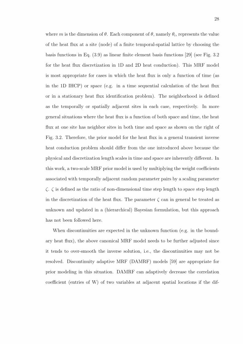
where m is the dimension of θ. Each component of θ, namely θi, represents the value
of the heat flux at a site (node) of a finite temporal-spatial lattice by choosing the
basis functions in Eq. (3.9) as linear finite element basis functions [29] (see Fig. 3.2
for the heat flux discretization in 1D and 2D heat conduction). This MRF model
is most appropriate for cases in which the heat flux is only a function of time (as
in the 1D IHCP) or space (e.g. in a time sequential calculation of the heat flux
or in a stationary heat flux identification problem). The neighborhood is defined
as the temporally or spatially adjacent sites in each case, respectively. In more
general situations where the heat flux is a function of both space and time, the heat
flux at one site has neighbor sites in both time and space as shown on the right of
Fig. 3.2. Therefore, the prior model for the heat flux in a general transient inverse
heat conduction problem should differ from the one introduced above because the
physical and discretization length scales in time and space are inherently different. In
this work, a two-scale MRF prior model is used by multiplying the weight coefficients
associated with temporally adjacent random parameter pairs by a scaling parameter
ζ. ζ is defined as the ratio of non-dimensional time step length to space step length
in the discretization of the heat flux. The parameter ζ can in general be treated as
unknown and updated in a (hierarchical) Bayesian formulation, but this approach
has not been followed here.
When discontinuities are expected in the unknown function (e.g. in the bound-
ary heat flux), the above canonical MRF model needs to be further adjusted since
it tends to over-smooth the inverse solution, i.e., the discontinuities may not be
resolved. Discontinuity adaptive MRF (DAMRF) models [59] are appropriate for
prior modeling in this situation. DAMRF can adaptively decrease the correlation
coefficient (entries of W) of two variables at adjacent spatial locations if the dif-

29
i-1
dt
neighbors of
i
t
qwi
i
i+1
qy
x
t
i
wi
Neighbors of
i
Figure 3.2: Linear finite element basis functions and neighborhood definition for θ.
The figure on the left refers to 1D heat conduction (unknown heat flux q(t)) and
the figure on the right to 2D heat conduction in a square domain (unknown heat
flux shown q(x, t)).
ference between these two variables tends to increase during the MCMC sampling
process. For instance, the correlation coefficient of two adjacent random variables
θi and θj can be defined as inversely proportional to |θi − θj| (i.e. the larger the
deviation between the two adjacent random variables, the smaller the spatial corre-
lation between them). As a consequence, the nonzero off-diagonal entries in W of
Eq. (3.12) vary in each MCMC sampling step instead of being fixed as −1. With
this consecutive update of the prior model (matrix W), the difference between two
adjacent variables tend to be amplified and the discontinuity, if there exists, will
eventually be resolved. For a complete summary and comparison of DAMRF mod-
els and the required programming techniques, one can consult [60]. In the current
study, a simple DAMRF model that mimics the basic line process model is adopted
[59]. In this approach, the total variation of θ is computed at each MCMC sam-
pling step after generating the new sample. If the variation between two adjacent
variables (say θi and θi+1) exceeds certain fraction (10% in current examples) of the
total variation, then Wi,i+1 and Wi+1,i are both set to zero, and 1 is subtracted from
30
ni and ni+1, respectively. Otherwise, the canonical MRF model is used. This model
is applied in Section 3.5 in the estimation of a discontinuous distributed heat source.
The prior distribution, p(k), of the conductivity is assumed to be of the form,
p(k) ∝ exp
−(k − k)2
2vk
, when k > 0, and 0 otherwise, (3.13)
where k and vk are the mean and variance, respectively, of a normal distribution.
This is in fact a renormalized normal distribution to enforce the non-negativity of
k. The uncorrelated joint normal distribution with mean d and covariance vdI is
assigned to d, where I is the identity matrix. Also, the state space of d is confined
in Ω.
3.2.3 The posterior distributions
With the above prior distribution models, the PPDF can be evaluated as,
p(θ, k,d|Y ) ∝ exp
−(Y − F (θ, k,d))T (Y − F (θ, k,d))
2vT
· exp
−1
2λθT Wθ
· exp
−(k − k)2
2vk
· exp
−(d− d)T (d− d)
2vd
,
k ∈ (0,∞) ∩ d ∈ Ω, and 0 otherwise. (3.14)
The parameters λ, k, vk, d and vd in the above formulation can be treated as ran-
dom variables in Bayesian inference, which are the hyper-parameters. A hierarchical
Bayesian PPDF is then formulated as follows:
p(θ, k,d, λ, k, vk, d, vd|Y ) ∝ p(Y |θ, k,d)p(θ|λ)p(k|k, vk)p(d|d, vd)
·p(λ)p(k)p(vk)p(d)p(vd). (3.15)
The function of this hierarchical Bayesian model is to diminish the effect of poor
prior knowledge of the hyper-parameters on the solution of the inverse problem. The

31
natural way to select priors for the hyper-parameters is to use the conjugate priors.
Hence, local uniform distributions are assigned to k and d. Gamma distribution
is chosen for λ, and inverse Gamma distribution is chosen for vk and vd. Equation
(3.15) can then be evaluated as,
p(θ, k,d, λ, k, vk, d, vd|Y ) ∝ exp
−(Y − F (θ, k,d))T (Y − F (θ, k,d))
2vT
·λm/2 exp−1
2λθT Wθ
v−1/2k exp
−(k − k)2
2vk
·v−r/2d exp
−(d− d)T (d− d)
2vd
λα0−1 exp −β0λ
·v−(1+α1)k exp
−β1v
−1k
v−(1+α2)d exp
−β2v
−1d
,
when λ ∈ (0,∞) ∩ k ∈ (0,∞) ∩ d ∈ Ω ∩ k ∈ (0, kmax] ∩ d ∈ Ω
∩ vk ∈ (0,∞) ∩ vd ∈ (0,∞), and 0 otherwise, (3.16)
where kmax is the maximum possible value of k (which can be an arbitrary large
number), r is the dimension of Ω, and (α0, β0), (α1, β1) and (α2, β2) are the parameter
pairs of the Gamma distribution that is of the form,
pX(x) =βα
Γ(α)xα−1e−βx, (3.17)
with Γ being the standard Gamma function. Here vT can also be treated as unknown
since it is rather difficult to quantify the magnitude of the measurement noise directly
from data. This is especially true when the experiment for collecting the temperature
data is not repetitive. In this case, the hierarchical and augmented Bayesian PPDF
is introduced as follows:
p(θ, k,d, λ, k, vk, d, vd, vT |Y ) ∝ v−n/2T exp
−(Y − F (θ, k,d))T (Y − F (θ, k,d))
2vT
·λm/2 exp−1
2λθT Wθ
v−1/2k exp
−(k − k)2
2vk

32
·v−r/2d exp
−(d− d)T (d− d)
2vd
λα0−1 exp −β0λ
·v−(1+α1)k exp
−β1v
−1k
v−(1+α2)d exp
−β2v
−1d
·v−(1+α3)T exp
−β3v
−1T
,
when λ ∈ (0,∞) ∩ k ∈ (0,∞) ∩ d ∈ Ω ∩ k ∈ (0, kmax] ∩ d ∈ Ω
∩ vk ∈ (0,∞) ∩ vd ∈ (0,∞) ∩ vT ∈ (0,∞), and 0 otherwise. (3.18)
Although the parameters k, d and θ are modeled as random variables in the same
joint distribution, there is no attempt to solve the inverse problem to simultaneously
estimate all these quantities. The solution to such a problem will, in most occasions,
be impractical or infeasible unless a substantial number of temperature data or
other constraints among the unknowns are available. Therefore, the idea behind
the above joint distribution is to investigate the effect of uncertainties in k and
d on the distribution of unknown θ provided prior distributions of k and d can
strongly constrain the highest density regions of k and d, respectively. Finally, it
is necessary to point out that the choices of distributions in the above formulations
are based on common practice but are not unique. The selection of distributions for
measurement noise and the priors may vary according to the nature of uncertainties
in each problem examined.
The above PPDFs are implicit due to the presence of numerical solver F , hence
can only be evaluated up to the normalizing constants. Numerical sampling strate-
gies are introduced in the next section to explore the posterior state spaces.
3.2.4 Regularization in the Bayesian approach
Before introducing the exploration of the posterior state space, it is helpful to discuss
the relation between Bayesian prior modeling and classical regularization method

33
for better understanding of the Bayesian method. Under some assumptions, one
can show that Bayesian prior regularization takes similar form to Tikhonov regular-
ization. For the system of Eq. (3.10), Tikhonov regularization modifies the original
finite dimensional parametric estimation problem posed with minimization of the
functional of Eq. (3.8) as follows:
θLS = argminθ 1
2‖F (θ)− Y ‖2
L2+ α‖θ‖2
p (3.19)
where θLS is the deterministic estimate of θ, α is a regularization parameter and ‖·‖p
represents different norms in the parameter space, usually taken as the L2 norm.
To clarify the relation between the above Tikhonov regularization and the Bayesian
prior regularization induced by Eq. (3.12), it is assumed that ωm is Gauss white
noise with known standard deviation σ. Then the likelihood function is the follow-
ing:
p(Y |θ) =1
(2πσ2)n/2exp−(F (θ)− Y )T (F (θ)− Y )
2σ2 (3.20)
where n = M ×N is the length of Y . The posterior PDF of θ can then be written
as follows:
p(θ|Y ) ∝ exp−(F (θ)− Y )T (F (θ)− Y )
2σ2
· λm/2 exp(−1
2λθT Wθ) (3.21)
From this distribution, the MAP estimate of θ can be derived as:
θMAP = argminθ 1
2(F (θ)− Y )T (F (θ)− Y ) +
λσ2
2θT Wθ (3.22)
By comparing Eqs. (3.19) and (3.22), it is seen that the least squares estimator and
the MAP estimator have similar mathematical forms. For example, by choosing
λ = 2ασ2 and W as an identity matrix, the two methods become identical for zeroth-
order Tikhonov regularization.

34
It is now clear that in Bayesian formulation, λ plays the role of a regularization
constant when σ is known. Different W ’s can be proposed for different problems.
One can in principle derive an MRF model to emulate various norms in the para-
meter space used in Tikhonov regularization.
In either approach, selection of regularization parameter, α or equivalently 12λσ2,
is important. There are in general three approaches for determining an optimal value
of regularization parameter. One is the so called Unbiased Predictive Risk Estimator
(UPRE) method. Another approach is the heuristic Tikhonov method, where the
inverse problem is solved with a set of regularization parameters. It was observed
that within a certain range of the regularization parameter (orders of magnitude
long), the obtained inverse solution was practically unchanged. The regularization
parameter is then chosen from this range. The third way, as used in this work, is
the use of a hierarchical Bayesian model. In this case, the problem is modeled in a
more flexible way and one is able to investigate uncertainty in spatial dependence
as well as to find the optimal regularization parameter.
3.3 Parameter estimation
In most cases, the thermophysical properties of conducting solids are not directly
measurable. Therefore, experiments are designed to measure closely related quan-
tities such as temperature. An inverse problem is then solved to obtain an optimal
estimate of the unknown property. Bayesian inference is applicable to this type
of inverse problem because the temperature is recognized as a sufficient statistic
of the thermophysical properties. Herein, thermal conductivity estimation is ana-
lyzed with the following analysis easily being extendable to the estimation of other
thermophysical properties.

35
Let us reconsider the inverse problems defined in Eqs. (3.1)-(3.9) with the mod-
ification that q0 and f are known and k is unknown. We also assume here that d is
fixed. According to Bayes’ formula, p(k|Y ) can be evaluated as,
p(k|Y ) ∝ p(Y |k)p(k). (3.23)
Therefore, as a special case of Eqs. (3.14), (3.16) and (3.18), the simple, hierar-
chical and augmented and hierarchical PPDFs of k conditional on the temperature
measurements Y are given as,
p(k|Y ) ∝ exp
−(Y − F (k))T (Y − F (k))
2vT
· exp
−(k − k)2
2vk
,
when k > 0, and 0 otherwise, (3.24)
p(k, k, vk|Y ) ∝ exp
−(Y − F (k))T (Y − F (k))
2vT
v−1/2k exp
−(k − k)2
2vk
·v−(1+α)k exp
−βv−1
k
, when k ∈ (0,∞) ∩ k ∈ (0, kmax]
∩vk ∈ (0,∞), and 0 otherwise, (3.25)
and,
p(k, k, vk, vT |Y ) ∝ v−n/2T exp
−(Y − F (k))T (Y − F (k))
2vT
·v−1/2k exp
−(k − k)2
2vk
v−(1+α)k exp
−βv−1
k
·v−(1+α1)T exp
−β1v
−1T
, when k ∈ (0,∞) ∩ k ∈ (0, kmax]
∩vk ∈ (0,∞) ∩ vT ∈ (0,∞), and 0 otherwise, (3.26)
respectively.
Equation (3.24) can be interpreted as a balance between prior belief regarding
the unknown parameter and information contained in the data (likelihood). More
precise prior models or more accurate measurements can lead to better posterior
estimates. Hence, the advantages of the above formulation over likelihood inference
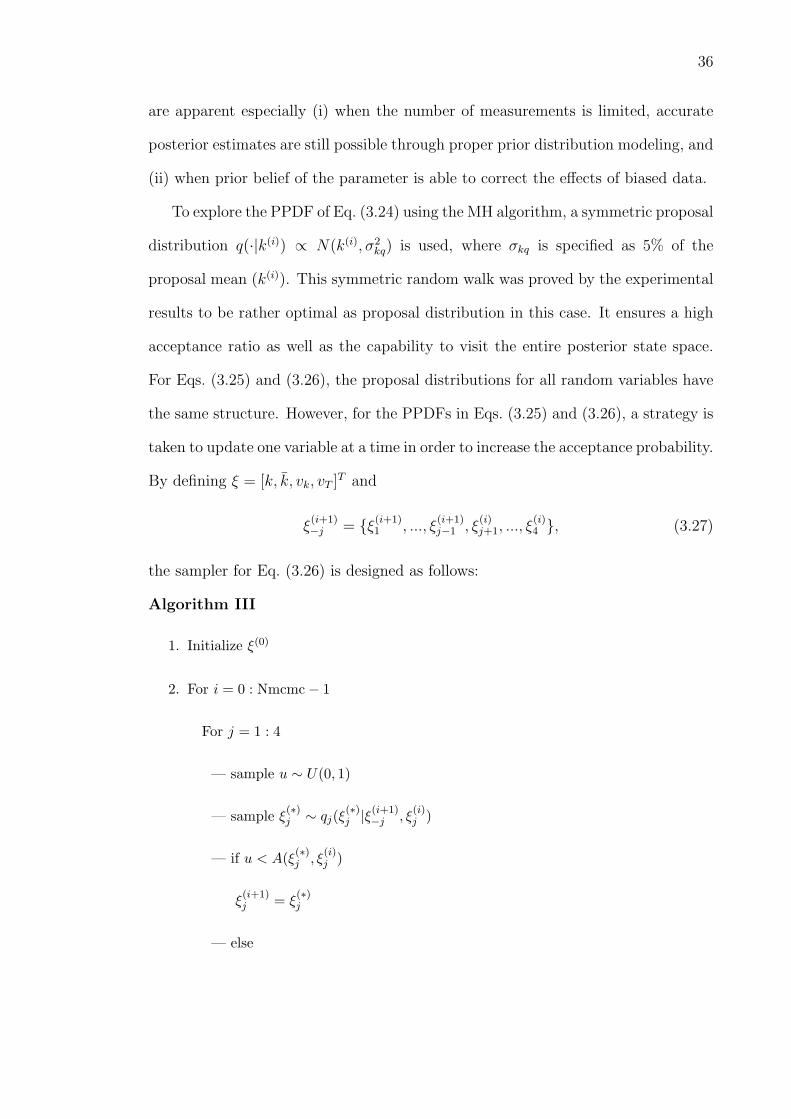
36
are apparent especially (i) when the number of measurements is limited, accurate
posterior estimates are still possible through proper prior distribution modeling, and
(ii) when prior belief of the parameter is able to correct the effects of biased data.
To explore the PPDF of Eq. (3.24) using the MH algorithm, a symmetric proposal
distribution q(·|k(i)) ∝ N(k(i), σ2kq) is used, where σkq is specified as 5% of the
proposal mean (k(i)). This symmetric random walk was proved by the experimental
results to be rather optimal as proposal distribution in this case. It ensures a high
acceptance ratio as well as the capability to visit the entire posterior state space.
For Eqs. (3.25) and (3.26), the proposal distributions for all random variables have
the same structure. However, for the PPDFs in Eqs. (3.25) and (3.26), a strategy is
taken to update one variable at a time in order to increase the acceptance probability.
By defining ξ = [k, k, vk, vT ]T and
ξ(i+1)−j = ξ(i+1)
1 , ..., ξ(i+1)j−1 , ξ
(i)j+1, ..., ξ
(i)4 , (3.27)
the sampler for Eq. (3.26) is designed as follows:
Algorithm III
1. Initialize ξ(0)
2. For i = 0 : Nmcmc− 1
For j = 1 : 4
— sample u ∼ U(0, 1)
— sample ξ(∗)j ∼ qj(ξ
(∗)j |ξ(i+1)
−j , ξ(i)j )
— if u < A(ξ(∗)j , ξ
(i)j )
ξ(i+1)j = ξ
(∗)j
— else

37
ξ(i+1)j = ξ
(i)j ,
where,
A(ξ(∗)j , ξ
(i)j ) = min
1,
p(ξ(∗)j |ξ(i+1)
−j )qj(ξ(i)j |ξ(∗)
j , ξ(i+1)−j )
p(ξ(i)j |ξ(i+1)
−j )qj(ξ(∗)j |ξ(i)
j , ξ(i+1)−j )
, (3.28)
and,
qj(ξ(∗)j |ξ(i+1)
−j , ξ(i)j ) ∝ N(ξ
(i)j , σ2
ξjq), (3.29)
where σξjq is 5% of the proposal mean (ξ(i)j ).
3.4 Heat flux reconstruction under uncertainties
Boundary heat flux reconstruction is possibly the most popular inverse problem
in heat transfer processes. In existing methods, the difficulty in selecting optimal
regularization parameter to obtain a point estimate has not been well addressed.
In addition, the effects of errors in thermophysical properties (e.g. conductivity
and specific heat) and sensor locations on the solution of the inverse problem were
not examined. Herein, these two issues are addressed separately in the hierarchical
Bayesian inference framework.
3.4.1 Automatic selection of the regularization parameter
Selection of the regularization parameter has never been a trivial problem in almost
all deterministic methods for inverse problems (e.g. in Tikhonov regularization [10]
or the iterative regularization method [3]). In Bayesian estimation, regularization
is still critical as the scaling parameter λ of the MRF prior, which acts as a regu-
larization parameter [29], affects the posterior distribution, and more explicitly, it
substantially affects the posterior point estimates. A hierarchical Bayesian method

38
provides an elegant approach to choose λ automatically based upon the noise level
and prior distribution models.
In this section, we consider the special cases of Bayesian formulations in Eqs. (3.16)
and (3.18) with assumptions that k and d are known fixed constants. The resulting
formulations are then PPDFs of boundary heat flux under measurement noise with
known or unknown vT . They are given as follows:
p(θ, λ|Y ) ∝ exp
−(Y − F (θ))T (Y − F (θ))
2vT
λm/2 exp
−1
2λθT Wθ
·λα0−1 exp −β0λ , when λ ∈ (0,∞), and 0 otherwise, (3.30)
p(θ, λ, vT |Y ) ∝ v−n/2T exp
−(Y − F (θ))T (Y − F (θ))
2vT
·λm/2 exp−1
2λθT Wθλα0−1 exp−β0λ
v−(1+α3)T exp
−β3v
−1T
,
when λ ∈ (0,∞) ∩ vT ∈ (0,∞), and 0 otherwise. (3.31)
These two hierarchical Bayesian formulations enable a mechanism to select λ au-
tomatically by treating λ as a random variable. In the MCMC exploration of the
above PPDFs, the parameter λ is updated in each iteration so that an optimal
distribution of λ conditional on the measurement data is achieved.
When k and d are fixed, the system equation can be simply written as:
Y = Hθ + TI + ω, (3.32)
where H is the sensitivity matrix:
H(j, k) = TH(tj; wk), j = 1 : n, k = 1 : m. (3.33)
In the above equation, TH denotes the direct simulation solution at sensor location
with zero initial condition, zero boundary conditions on Γg and Γh, and heat flux wk

39
on Γ0. Also, TI denotes the direct solution at sensor location with zero boundary
condition on Γo and known initial condition and boundary conditions on Γg and Γh,
respectively.
In this case, it is noticed that the conditional distribution of θ on λ, vT and
Y follows a multivariate Gaussian. Hence, the full conditional distribution of each
component of θ is in standard form, which can be derived as follows:
p(θi|θ−i, λ, vT , Y ) ∝ N(µi, σ2i ), µi =
bi
2ai
, σi =
√1
ai
,
ai =N∑
s=1
H2si
vT
+ λWii, bi = 2N∑
s=1
µsHsi
vT
− λµp,
µs = Ys − (TI)s −∑
t6=i
Hstθt, µp =∑
j 6=i
Wjiθj +∑
k 6=i
Wikθk. (3.34)
It was mentioned earlier that the full conditional distribution can be used as proposal
distribution in the MCMC sampler. This will lead to a single-component Gibbs
sampler that has acceptance probability 1.0. A modified single-component Gibbs
sampler is thus used to explore the PPDFs in Eqs. (3.30) and (3.31) as follows,
Algorithm IV
1. Initialize θ(0), λ(0) and v(0)T
2. For i = 0 : Nmcmc− 1
— sample θ(i+1)1 ∼ p(θ1|θ(i+1)
−1 , λ(i), v(i)T )
— sample θ(i+1)2 ∼ p(θ2|θ(i+1)
−2 , λ(i), v(i)T )
—...
— sample θ(i+1)m ∼ p(θm|θ(i+1)
−m , λ(i), v(i)T ).
— sample u ∼ U(0, 1)
— sample λ(∗) ∼ qλ(λ(∗)|λ(i))

40
— if u < A(λ(∗), λ(i))
λ(i+1) = λ(∗)
— else
λ(i+1) = λ(i),
— sample u ∼ U(0, 1)
— sample v(∗)T ∼ qv(v
(∗)T |v(i)
T )
— if u < A(v(∗)T , v
(i)T )
v(i+1)T = v
(∗)T
— else
v(i+1)T = v
(i)T ,
where qλ and qv are determined similarly to Eq. (5.29).
3.4.2 Effect of the sensor location
In the proceeding sections, the focus was given to exploring the statistical informa-
tion of measurement errors and the prior modeling of primary- and hyper-unknowns.
However, other factors may also affect the solution of inverse heat conduction prob-
lems. Since the inverse problems are driven by sensor data, it is rational to in-
vestigate the effect of sensor location on the solution of the inverse problem. It is
straightforward to realize that the closer the sensor to the boundary, the better the
point estimate of the boundary heat flux is. However, the question of how the loca-
tion affects the higher order statistics of the boundary heat flux, or more specifically,
how the reliability regions of the inverse solution are affected by the sensor location,
can only be answered through Bayesian computation.

41
The difficulty of analyzing the effect of sensor location arises from the fact that
for the majority of inverse problems of interest, there is no closed functional form
available to describe the relation between d and the statistics of the inverse solutions
or even the point estimates themselves. For instance, in Eq. (3.33), d affects each
component of the sensitivity matrix H; hence it also affects the PPDF in Eq. (3.31).
However, it is rather difficult to explicitly study the effect of d on the posterior dis-
tribution of θ in an analytical manner. An alternative approach is to investigate the
effect by Bayesian computation. Given the PPDF of Eq. (3.31) and same magnitude
of the measurement noise, a sequence of numerical experiments can be conducted
with different sensor locations d1, d2, . . ., ds. By comparing the posterior estimates
(both point estimates and probability bounds) from MCMC samples, the effect of
d can be revealed. This experimental method provides an approach to guide ex-
perimental design in data-driven inverse problems, especially for higher dimensional
problems where it is of practical importance to use a minimum number of sensors
to achieve desirable inverse solution accuracy and reliability.
3.4.3 IHCP under model uncertainties
In many boundary heat flux reconstruction problems, the knowledge of thermophys-
ical property and/or sensor location is not exact. For instance, the true values of k
and d may exist in a narrow neighborhood of the nominal values. It is not clear up
to now how the uncertainties (small errors) in these system parameters would affect
the inverse solutions and the PPDF. Once again, as mentioned in the discussion
of the sensor location effect, it is impossible to conduct the investigation analyt-
ically. Therefore, the proposed approach is to explore the hierarchical Bayesian
formulation.

42
In Eq. (3.18), all hyper-parameters are modeled as random variables. Although
reasonable from a statistical inference perspective, the exploration of this formula-
tion can only be physically feasible by constraining the prior distributions of k and
d. Let us consider the practical case where k and d are known to be around certain
nominal values. In this case, constraints can be added to Eq. (3.18) by setting k
and d as the nominal values. Following these assumptions, the PPDF to investigate
effects of system uncertainties is,
p(θ, k,d, λ, vk, vd, vT |Y ) ∝ v−n/2T exp
−(Y − F (θ, k,d))T (Y − F (θ, k,d))
2vT
·λm/2 exp−1
2λθT Wθ
v−1/2k exp
−(k − k)2
2vk
·v−r/2d exp
−(d− d)T (d− d)
2vd
λα0−1 exp −β0λ
·v−(1+α1)k exp
−β1v
−1k
v−(1+α2)d exp
−β2v
−1d
·v−(1+α3)T exp
−β3v
−1T
,
when λ ∈ (0,∞) ∩ k ∈ (0,∞) ∩ d ∈ Ω ∩ vk ∈ (0,∞) ∩ vd ∈ (0,∞)
∩ vT ∈ (0,∞), and 0 otherwise. (3.35)
For this PPDF, the sensitivity matrix H varies in each MCMC iteration since
k and d are updated as well. Therefore, in implementations of the modified single-
component Gibbs sampler (algorithm IV), the sensitivity matrix H needs to be
recomputed at each iteration using updated k and d. H is used to update θ in the
single-component Gibbs sampling algorithm, and then the other random variables
λ, k, d, vk, vd and vT are updated consecutively in each MCMC step. Another mod-
ification to algorithm IV is that the proposal distributions of k and d are N(k, vk)
and N(d, vdI) in each iteration, respectively. Solutions of the IHCP accounting for
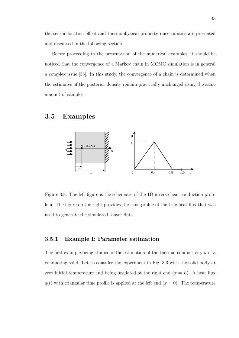
43
the sensor location effect and thermophysical property uncertainties are presented
and discussed in the following section.
Before proceeding to the presentation of the numerical examples, it should be
noticed that the convergence of a Markov chain in MCMC simulation is in general
a complex issue [38]. In this study, the convergence of a chain is determined when
the estimates of the posterior density remain practically unchanged using the same
amount of samples.
3.5 Examples
xq
dL
Y (d,i
t)
q
t0 0.4 0.8
1
1.0
Figure 3.3: The left figure is the schematic of the 1D inverse heat conduction prob-
lem. The figure on the right provides the time-profile of the true heat flux that was
used to generate the simulated sensor data.
3.5.1 Example I: Parameter estimation
The first example being studied is the estimation of the thermal conductivity k of a
conducting solid. Let us consider the experiment in Fig. 3.3 with the solid body at
zero initial temperature and being insulated at the right end (x = L). A heat flux
q(t) with triangular time profile is applied at the left end (x = 0). The temperature

44
Table 3.1: Bayesian estimates of k using different models.
case# Bayesian model prior of k data # σT kpostmean σk
1 Simple (Eq. 3.24) normal 50 0.005 1.2210 0.0032
2 Simple (Eq. 3.24) normal 50 0.001 1.2150 0.0006
3 Simple (Eq. 3.24) normal 100 0.005 1.2166 0.0022
4 Simple (Eq. 3.24) uniform 50 0.005 1.2205 0.0031
5 Hierarchical (Eq. 3.25 normal 50 0.005 1.2204 0.0031
with vk known)
6 Hierarchical (Eq. 3.25) normal 50 0.005 1.2204 0.0032
7 Hierarchical (Eq. 3.26) normal 50 0.005 1.2206 0.0058
is recorded at x = d. To simplify the discussion, the numerical study is conducted
in a dimensionless manner as follows:
∂T
∂t= k
∂2T
∂x2, 0 < t < 1, 0 < x < 1, (3.36)
T (x, 0) = 0, 0 ≤ x ≤ 1, (3.37)
k∂T
∂x|x=1 = 0, k
∂T
∂x|x=0 = q(t), 0 < t < 1. (3.38)
The simulation data are generated by adding i.i.d. Gauss random noise with mean
0 and variance vT to the computed temperature at d. In generating the data, a true
value of k is used randomly generated from a normal distribution with mean k and
variance vk (standard deviation σk). Algorithm III is used in this example. The
parameters α, β, α1 and β1 all take values of 1.0e− 3.
In this example, k and σk are taken as 1.0 and 0.15, respectively, and a value of
1.2146 is generated as the true k. In Table 1, the Bayesian estimates using differ-
ent formulations and different simulation data are listed. kpostmean is the posterior

45
mean estimate and σk is the estimate of standard deviation of the posterior dis-
tribution. The posterior densities of k in all listed cases are plotted in Fig. 3.4.
For each case, 20000 samples (after convergence) generated by the MH sampler are
used to compute the estimates. It is clear that the posterior mean estimates are
largely accurate. Note that increasing the number of measurements or decreasing
1.20 1.21 1.22 1.23 1.240
200
400
600
1.20 1.21 1.22 1.23 1.240
200
400
600
1.20 1.21 1.22 1.23 1.240
200
400
600
1.20 1.21 1.22 1.23 1.240
200
400
600
1.20 1.21 1.22 1.23 1.240
200
400
600
1.20 1.21 1.22 1.23 1.240
200
400
600
1.20 1.21 1.22 1.23 1.240
200
400
600
case 1 case 2 case 3
case 4 case 5 case 6
case 7
Figure 3.4: Computed posterior densities of k using different Bayesian models.
the magnitude of measurement errors can both reduce the standard deviation of
the posterior distribution and improve the posterior mean estimate. The posterior
mean estimate obtained from the first case is slightly more biased than the other
cases since the normal prior (fixed mean 1.0 and standard deviation 0.15) is biased
in representing the true value of k while the data contain more accurate information
about k. By relaxing the prior assumption on k, the estimates are improved. In
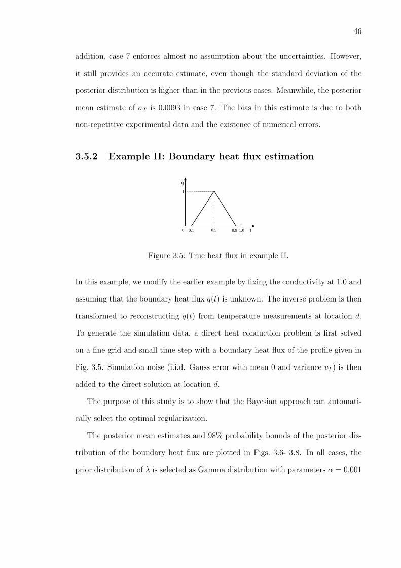
46
addition, case 7 enforces almost no assumption about the uncertainties. However,
it still provides an accurate estimate, even though the standard deviation of the
posterior distribution is higher than in the previous cases. Meanwhile, the posterior
mean estimate of σT is 0.0093 in case 7. The bias in this estimate is due to both
non-repetitive experimental data and the existence of numerical errors.
3.5.2 Example II: Boundary heat flux estimation
q
t0 0.5 0.9
1
1.00.1
Figure 3.5: True heat flux in example II.
In this example, we modify the earlier example by fixing the conductivity at 1.0 and
assuming that the boundary heat flux q(t) is unknown. The inverse problem is then
transformed to reconstructing q(t) from temperature measurements at location d.
To generate the simulation data, a direct heat conduction problem is first solved
on a fine grid and small time step with a boundary heat flux of the profile given in
Fig. 3.5. Simulation noise (i.i.d. Gauss error with mean 0 and variance vT ) is then
added to the direct solution at location d.
The purpose of this study is to show that the Bayesian approach can automati-
cally select the optimal regularization.
The posterior mean estimates and 98% probability bounds of the posterior dis-
tribution of the boundary heat flux are plotted in Figs. 3.6- 3.8. In all cases, the
prior distribution of λ is selected as Gamma distribution with parameters α = 0.001

47
0 0.1 0.2 0.3 0.4 0.5 0.6 0.7 0.8 0.9 1
−0.2
0
0.2
0.4
0.6
0.8
1
1.2
t
q
True heat fluxPosterior mean estimate98% probability bounds
0 0.1 0.2 0.3 0.4 0.5 0.6 0.7 0.8 0.9 1−0.4
−0.2
0
0.2
0.4
0.6
0.8
1
1.2
t
q
True heat fluxPosterior mean estimate98% probability bounds
Figure 3.6: Posterior mean estimates of the heat flux and 98% probability bounds
of the posterior distributions when d = 0.5 using a hierarchical Bayesian model
(Example II). The figure on the left is obtained when σT = 0.01 and the figure on
the right is obtained when σT = 0.001.
and β = 0.001. This prior barely contains any information regarding λ except
for enforcing its nonnegativity. 100 measurements are taken at the sensor location
(sampling time interval ∆t = 0.01) for all cases. The results in Figs. 3.6 and 3.8 are
obtained when the thermocouple is located at d = 0.5, and the ones in Fig. 3.7 are
obtained when d = 0.1. Two levels of noise are considered, σT = 0.01 and 0.001. In
the discretization of q(t), 51 basis functions are used for each case. The hierarchical
Bayesian model of Eq. (3.30) is used to obtain the results in Figs. 3.6 and 3.7, and
the hierarchical and augmented Bayesian model of Eq. (3.31) is used to obtain the
results in Fig. 3.8. For all cases, 50000 MCMC samples are generated and the results
are obtained from the last 25000 samples.
It is clear that the automatic selection of the regularization parameter using
the hierarchical Bayesian model is rather optimal. The posterior estimates in all
cases are accurate and stable to perturbations in the location of the thermocouple
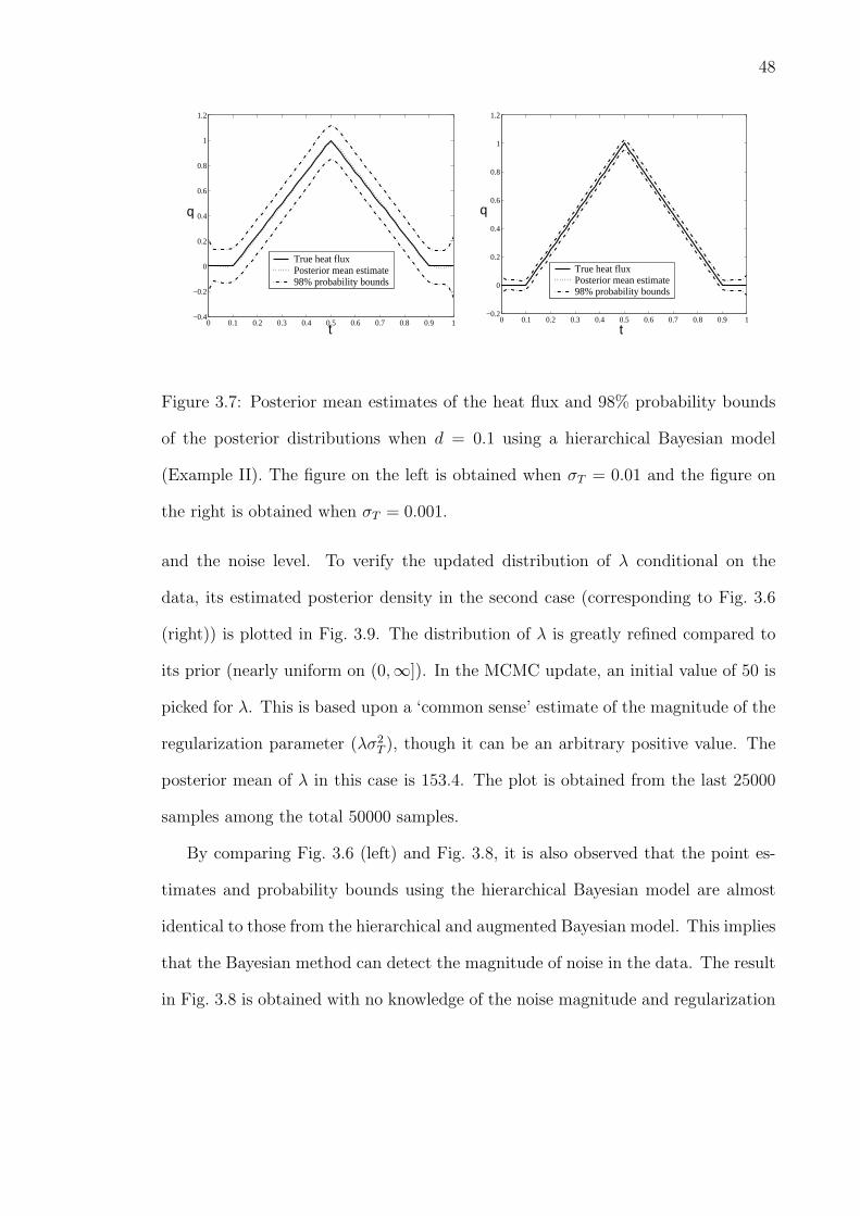
48
0 0.1 0.2 0.3 0.4 0.5 0.6 0.7 0.8 0.9 1−0.4
−0.2
0
0.2
0.4
0.6
0.8
1
1.2
t
q
True heat fluxPosterior mean estimate98% probability bounds
0 0.1 0.2 0.3 0.4 0.5 0.6 0.7 0.8 0.9 1−0.2
0
0.2
0.4
0.6
0.8
1
1.2
t
q
True heat fluxPosterior mean estimate98% probability bounds
Figure 3.7: Posterior mean estimates of the heat flux and 98% probability bounds
of the posterior distributions when d = 0.1 using a hierarchical Bayesian model
(Example II). The figure on the left is obtained when σT = 0.01 and the figure on
the right is obtained when σT = 0.001.
and the noise level. To verify the updated distribution of λ conditional on the
data, its estimated posterior density in the second case (corresponding to Fig. 3.6
(right)) is plotted in Fig. 3.9. The distribution of λ is greatly refined compared to
its prior (nearly uniform on (0,∞]). In the MCMC update, an initial value of 50 is
picked for λ. This is based upon a ‘common sense’ estimate of the magnitude of the
regularization parameter (λσ2T ), though it can be an arbitrary positive value. The
posterior mean of λ in this case is 153.4. The plot is obtained from the last 25000
samples among the total 50000 samples.
By comparing Fig. 3.6 (left) and Fig. 3.8, it is also observed that the point es-
timates and probability bounds using the hierarchical Bayesian model are almost
identical to those from the hierarchical and augmented Bayesian model. This implies
that the Bayesian method can detect the magnitude of noise in the data. The result
in Fig. 3.8 is obtained with no knowledge of the noise magnitude and regularization

49
0 0.1 0.2 0.3 0.4 0.5 0.6 0.7 0.8 0.9 1
−0.2
0
0.2
0.4
0.6
0.8
1
t
q
True heat fluxPosterior mean estimate98% probability bounds
Figure 3.8: Posterior mean estimates of the heat flux and 98% probability bounds
of the posterior distribution when d = 0.5 and σT = 0.01 using a hierarchical and
augmented Bayesian model (Example II).
50 100 150 200 250 3000.000
0.004
0.008
0.012
0.016
p()
Figure 3.9: Posterior density estimate of hyper-parameter λ in the second case.

50
parameter. This example demonstrates the advantages of using the Bayesian infer-
ence method for inverse problem solution. By comparing Figs. 3.6 and 3.7, it is also
observed that the distribution (probability bounds) of the heat flux conditional on
the temperature measurements is affected significantly not only by the noise level
but also by the location of the thermocouple. At the same noise level, the closer the
sensor is to the boundary with unknown heat flux, the narrower the highest density
region of the posterior state space.
3.5.3 Example III: Boundary heat flux identification with
simultaneous uncertainties in material property and
thermocouple location
0 0.1 0.2 0.3 0.4 0.5 0.6 0.7 0.8 0.9 1
−0.2
0
0.2
0.4
0.6
0.8
1
t
q
True heat fluxPosterior mean estimate98% probability bounds
0 0.1 0.2 0.3 0.4 0.5 0.6 0.7 0.8 0.9 1
−0.2
0
0.2
0.4
0.6
0.8
1
t
q
True heat fluxPosterior mean estimate98% probability bounds
Figure 3.10: Posterior mean estimates of the heat flux and 98% probability bounds
of the posterior distribution when uncertainties in d and k exist. The figure on the
left is obtained using true d and k, and the figure on the right is obtained using the
nominal values of d and k (Example III).
In the third numerical experiment, the 1D inverse heat conduction problem is
reconsidered with uncertainties in the thermal conductivity k and sensor location d.

51
0 0.1 0.2 0.3 0.4 0.5 0.6 0.7 0.8 0.9 1
−0.2
0
0.2
0.4
0.6
0.8
1
t
q
True heat fluxPosterior mean estimate98% probability bounds
Figure 3.11: Posterior mean estimates of the heat flux and 98% probability bounds
of the posterior distribution when k and d are treated as random variables (Example
III).
It is thus assumed that the true values of k and d are near known nominal values k
and d for the given experiment, respectively. It is of interest to study the effect of
such system uncertainties on the computed inverse solutions.
In the current cases, k and d are selected as 1.0 and 0.3, respectively (dimension-
less quantities). Two random values 0.968376 and 0.328135 are generated to act as
the true values of k and d, respectively. 100 simulation measurements are generated
using the true k and d and the heat flux profile in the right Fig. 3.3 following the
same procedure as in the earlier examples. Also, σT = 0.005 in this part of the
study. First, two cases are studied as shown in Fig. 3.10. The results are obtained
through exploring the PPDF in Eq. (3.31) using the sensitivity matrix H computed
at nominal values k and d (right figure) and at true values k and d (left figure). The
third case is conducted through exploring the PPDF in Eq. (3.35) in which k and
d are treated as random variables (Fig. 11). It is observed from the three plots in
Figs. 3.10 and 11 that the uncertainties in k and d do not significantly affect the

52
inverse solution (posterior distribution). However, this is based upon the fact that
the magnitude of the uncertainties considered is small. In this case, the distribution
of the inverse solution is mainly dominated by the measurement noise.
3.5.4 Example IV: 1D piece-wise continuous heat source
identification
A heat source identification problem in 1D heat conduction is examined in this
section. The problem has been studied by Yi and Murio [15] using the mollification
method [61]. It is defined in a dimensionless manner as:
∂T
∂t= (k(x)Tx)x + f(x, t), (3.39)
where f(x, t) is the unknown source function to be estimated from temperature
measurements. As in Yi and Murio [15], we examine the following special case: when
k(x)=1 in x ∈ [0, 0.25], k(x) = 4x in x ∈ [0.25, 0.5], k(x) = 3− 2x in x ∈ [0.5, 0.75]
and k = 1.5 in x ∈ [0.75, 1.0], and T (x, t) = ex−t in x ∈ [0, 1], the exact heat source
is given as f(x, t) = −2ex−t in x ∈ [0, 0.25], f(x, t) = −(5+4x)ex−t in x ∈ [0.25, 0.5],
f(x, t) = (−2 + 2x)ex−t in x ∈ [0.5, 0.75] and f(x, t) = −2.5ex−t in x ∈ [0.75, 1.0].
We use the PPDF in Eq. (3.31) to solve these two problems by replacing the heat
flux term with the heat source term. The line process DAMRF model is used as prior
distribution of the heat source. The simulation data are generated by adding i.i.d.
Gauss random errors with σT = 0.005 to the analytical T (x, t). The temperature
is assumed to be measured at 31 evenly distributed sites within the domain [0, 1]
(no sensors on the boundary) at constant sampling time interval of 0.01. A grid
with 128 elements is used in the discretization of the heat source. The heat source
is reconstructed from t = 0 to t = 0.5. The true heat source and posterior mean

53
estimate are plotted in Fig 3.12. The results are rather accurate and comparable
with the results achieved in [15] under similar conditions except that the number of
thermocouples used in the current example is significantly less.
00.2
0.40.6
0.81 0
0.1
0.2
0.3
0.4
0.5
−15
−10
−5
0
y
x
f
00.2
0.40.6
0.81 0
0.1
0.2
0.3
0.4
0.5
−15
−10
−5
0
y
x
f
Figure 3.12: True heat source (left) and reconstructed heat source (right) for case
II of Example IV.
To verify the accuracy of the posterior mean estimates, the estimates and 98%
probability bounds of the posterior distributions at t=0.24 are plotted in Fig. 13.
0 0.1 0.2 0.3 0.4 0.5 0.6 0.7 0.8 0.9 1−12
−10
−8
−6
−4
−2
0
x
f
True heat source Posterior mean estimate98% probability bounds of the posterior distribution
Figure 3.13: Posterior mean estimate and 98% probability bounds of the posterior
distribution of step heat source at t = 0.24.

54
3.5.5 Example V: 2D heat source identification
In this example, we consider a heat source identification problem as follows,
∂T
∂t=
∂2T
∂x2+
∂2T
∂y2+ f(x, y, t), 0 < t, 0 < x, y < 1, (3.40)
T (x, y, 0) = 0, 0 ≤ x, y ≤ 1, (3.41)
∂T
∂x|x=0 =
∂T
∂y|y=0 =
∂T
∂x|x=1 =
∂T
∂y|y=1 = 0, 0 < t, (3.42)
where the heat source f(x, y, t) is unknown. The problem is to reconstruct this
temporal-spatially varying quantity from temperature measurements at a number
of sensor locations.
0 0.5 100.5
10
100
200
xy
f
0 0.5 10
0.5
10
100
200
xy
f
0 0.5 10
0.5
10
100
200
xy
f
0 0.5 100.5
10
100
200
xy
f
t = 0 t = 0.02
t = 0.05 t = 0.1
Figure 3.14: True heat source profiles for example V.
A numerical experiment is conducted by simulating the case where 25 thermo-
couples are uniformly distributed within the domain [0, 1]×[0, 1], which is considered
a reasonable setup since no information about the heat source distribution is avail-
able a priori. At each sensor location, 20 measurements are taken at equal frequency
from t = 0 to t = 0.1.

55
0 0.5 100.5
10
100
200
xy
f
0 0.5 100.5
10
50
100
150
200
250
xy
f
0 0.5 100.5
10
100
200
xy
f
0 0.5 100.5
10
100
200
xy
f
t = 0 t = 0.02
t = 0.05 t = 0.1
Figure 3.15: Posterior mean estimates of heat source profiles when σT = 0.02 for
example V.
The true heat source used in the simulation data generation is of the form
f(x, y, t) = exp(−10t)20
2π · 0.1252exp
−(x− 0.75)2 + (y − 0.725)2
2 · 0.1252
. (3.43)
The data are generated by adding i.i.d. Gauss random errors (0 mean and standard
deviation σT ) to the direct solution with this heat source on a fine finite element
grid. Two magnitudes of noise level with σT = 0.005 and 0.02, respectively, are
examined.
This example is solved using the Bayesian formulation in Eq. (3.31). The two-
scale MRF model is used in prior modeling of the heat source. The heat source is
reconstructed using a discretization of 32× 32 grid in space and 11 basis functions
in time. The posterior state space is explored using the modified single-component
Gibbs sampler (algorithm IV).
The true heat source profiles at different time points and corresponding recon-
structed heat source profiles (posterior mean estimates) in the second case (σT =
0.02) are plotted in Figs. 3.14 and 3.15, respectively. It is seen that the posterior

56
mean estimates are overall rather accurate. The deviations in estimates at the ini-
tial time and the final time points are slightly larger. This is because the noise
to signal ratio in the first few time steps is large, and the simulated data contains
less information regarding the heat source in the final time period. Considering the
uniform distribution of sensors and the fact that no assumptions on noise magnitude
and regularization parameter are made in the solution procedure, the estimates are
rather satisfactory.
To further verify the accuracy of the posterior mean estimate, the reconstructed
heat source profiles at y = 0.725 at different time steps are plotted in Fig. 16 for
the first case (σT = 0.005). The probability bounds for the posterior distribution at
t = 0.05 are also shown in the same figure. It is seen that the estimates are rather
accurate except at early times as discussed above.
0 0.1 0.2 0.3 0.4 0.5 0.6 0.7 0.8 0.9 1
−50
0
50
100
150
200
x
f
true heat source
posterior mean estimate
t = 0
t = 0.05
t = 0.1
t = 0.02
98% probability boundsof posterior distributionat t=0.05
Figure 3.16: Computed heat source at y = 0.725 at different times (example V, σT =
0.005). Also shown are the 98% probability bounds of the posterior distribution at
t = 0.05.

57
3.6 Summary
In this chapter, the Bayesian computational approach using hierarchical Bayesian
formulations and MCMC simulation is presented for the solution of stochastic in-
verse problems in heat conduction. It has been demonstrated through numerical
examples that the Bayesian computational approach provides means to quantify
various system uncertainties and to deduce accurate probabilistic specifications of
the inverse solutions. In all presented numerical studies, the direct problems were
solved on much finer finite element grids and using smaller time steps than the dis-
cretization used in computing the inverse solutions. Still the discretization used in
the inverse solutions was fine enough to diminish the regularization effect introduced
by the a priori assumed function specification.
The fundamental steps of using Bayesian statistics to solve inverse continuum
problems and the advantages of Bayesian computational approach in quantifying un-
certainty, resolving discontinuity and selecting regularization parameter are demon-
strated via studies in this chapter.

Chapter 4
Inverse heat radiation problem
(IHRP)- An integrated
reduced-order modeling and
Bayesian computational approach
to complex inverse continuum
problems
In the previous chapter, the basic Bayesian computational approach to inverse con-
tinuum problems has been demonstrated via application to IHCP. However, the
algorithms developed in the previous chapter are fairly expensive to implement for
inverse problems in complex nonlinear PDE systems. For the purpose of addressing
the high computational cost of Bayesian computational method to inverse problems,
58

59
a reduced-order modeling approach is introduced in this chapter to integrate with
MCMC algorithms. This unique combination allows the solution to complex inverse
continuum problems. The reduced-order modeling method is based on the proper
orthogonal decomposition (POD) [62] and is illustrated via an inverse heat radiation
problem (IHRP) herein. As demonstrated in the numerical example, the simulation
time is drastically reduced using the POD method in the inverse computation.
The remaining of this chapter is organized in the following sequence. Section
4.1 introduces the inverse heat radiation problem. Section 4.2 briefly describes
the full- and reduced-order finite element models used for the direct analysis. The
formulation of the likelihood is presented in Section 4.3 together with the prior
distribution model and the PPDF under a Bayesian inference framework. The design
of the MCMC sampler is discussed in Section 4.4 including the exploration of the
posterior state space. In Section 4.5, two examples of reconstruction of step and
triangular heat source profiles are provided. Finally, Section 4.6 summarizes the
observations of this numerical study and some related issues.
4.1 The inverse heat radiation problem (IHRP)
Study of thermal radiation has been motivated by a wide range of applications in-
cluding thermal control in space technology, combustion, high temperature forming
and coating technology, solar energy utilization, high temperature engine, furnace
technology and other [63]. In participating media, radiation is accompanied by
heat conduction and convection. To simulate such processes, a coupled system
of partial differential equations (PDEs) governing temperature and radiation in-
tensity evolution needs to be solved iteratively. Difficulties arise in the solution
of such systems because the heat flux contributed by radiation varies nonlinearly

60
with the temperature, the radiation intensity varies in space and in direction, and
the radiation intensity equation is an integro-differential equation [63]. The direct
radiation problem, in which the temperature distribution is computed with pre-
scribed thermal properties, source generation and initial/boundary conditions, is
often solved using a combination of spatial discretization methods such as finite
volume or finite element methods (FEM) and ordinate approximation such as PN
and SN methods [63]. The inverse radiation problem in a participating medium that
is of interest here is defined as reconstruction of the heat source given temperature
measurements within the domain [64, 65, 66]. Similar problems have been studied
in [67, 68, 69, 70, 71, 72] using gradient based optimization methods of least-squares
error objection function/functional. Other methods, such as Monte Carlo method,
have also been developed for solving inverse radiation problems [73].
In this work, the situation where thermal conduction and radiation occur simul-
taneously in a participating medium with diffusively reflecting gray boundaries is
considered. The schematic of the problem of interest is given in Fig. 4.1. Inside the
3D domain V , heat conduction occurs simultaneously with absorption, scattering
and emission of the electromagnetic waves. On the boundary surface S, the temper-
ature is known and the electromagnetic waves are diffusively reflected. The transient
heat source will be estimated through temperature measurements at sensor (ther-
mocouple) sites within the domain. The governing equations for the temperature
and radiation intensity evolution in the domain V are as follows:
ρCp∂T
∂t= k∇2T −∇ · ~qr + g(t)G(x− x∗, y − y∗, z − z∗) (4.1)
~s · ∇I + (κ + σ)I − σ
4π
∫
4πI(~r, ~s
′)dΩ
′= κIb (4.2)

61
n
n
heat source
*
**
thermocouple
* S (diffusively reflecting,T known)
V
x
yz
Figure 4.1: Schematic of the inverse radiation problem. The objective is to compute
the point heat source g(t) given initial conditions, boundary conditions on the surface
and temperature measurements at a number of points within the domain.
where Ib is the black body radiation intensity governed by Planck function,
Ib =σbT
4
π(4.3)
and ~qr is the heat flux contributed by radiation:
∇ · ~qr = 4πκ(Ib − 1
4π
∫
4πI(~r, ~s)dΩ) (4.4)
On the boundary S, the following holds:
I(~r, ~s) = εIb +1− ε
π
∫
~n·~s′<0|~n · ~s′|I(~r, ~s
′)dΩ
′~n · ~s > 0 (4.5)
T = Tw (4.6)
In the above equations, T and I denote the temperature and radiation intensity,
respectively, ~r is the position vector and ~s is the direction vector. G(x − x∗, y −y∗, z− z∗) is the spatial approximation of a point heat source located at (x∗, y∗, z∗).
In this work, a 3D Gaussian distribution function is used for G. Ω stands for the
solid angle over the entire space. ρ is the density of the medium, Cp is the thermal
capacity, k is the thermal conductivity, and κ, σ, ε are the absorption coefficient,
scattering coefficient and boundary wall emissivity, respectively. Finally, σb is the

62
Stefan-Boltzmann constant and ~n is the unit normal vector on S pointing into the
domain.
In the inverse problem of interest, the heat source g(t) is the main unknown. Its
calculation becomes feasible by providing the values of the temperature at a given
number of locations within the domain as shown in Fig. 4.1. As in the discussion
of IHCP, let Y denote the measured temperature data. The inverse problem is then
stated as follows: find an estimate g(t) of the real heat source g(t) such that the
computed temperatures with this optimal source estimate can match Y in some
sense. For instance, most deterministic approaches will solve for g(t) by minimizing
the least-squares error between Y and the computed temperatures.
4.2 Direct simulation and reduced-order model-
ing
The direct problem can be solved using a combination of the finite element method
(FEM) in space discretization and the S4 method in ordinate discretization. It is
seen that Eq. (4.1) is a nonlinear partial differential equation (PDE) and Eq. (4.2)
has an integral term. They are coupled by the expressions in Eqs. (4.3) and (4.4).
The iterative process at each time step to solve the coupled Eqs. (4.1) and (4.2) is
summarized next:
1. Set T(i)guess = T (i−1);
2. Substitute T(i)guess into Eq. (4.3) to compute Ib;
3. Solve Eq. (4.2) for I(i);
4. Use Eq. (4.4) to compute ∇ · ~qr;

63
5. Solve Eq. (4.1) and update T(i)guess with the solution;
6. If the solutions converged, set T(i)guess as T (i) and save I(i); otherwise, go to step 2.
7. Go to the next time step.
Here T (i) denotes the temperature solution at the ith time step (note that T (0) is
a known initial temperature field) and T (i)guess is the guessed temperature solution.
In each iteration of the above procedure, the integro-differential Eq. (4.2) is solved
using the S4 method [63]. In this approach, the intensity I at each spatial point
is discretized into 24 directions. The integration over solid angles (directions) is
approximated as weighted sum in these 24 directions. The direction vectors and
associated weights are specified in [63]. In each direction, the governing equation
for I can be written as follows:
~si · ∇Ii + (κ + σ)Ii − σ
4π
24∑
j=1
Ij(~r)wj = κIb (4.7)
The associated boundary condition takes the following form:
Ii = εIb +1− ε
π
∑
j: ~n·~sj<0|~n · ~sj|wjIj, ~n · ~si > 0 (4.8)
where wj is the weight associated with the jth direction. For any given temperature
field, 24 equations as Eq. (4.7) with fixed direction vectors, ~si’s, need to be solved
iteratively to obtain I. It is noticed that Eq. (4.7) contains an advection term
~si · ∇Ii, hence the streamline-upwind/Petrov-Galerkin (SUPG) formulation [74] is
used to derive stabilized FEM equations. In summary, the weak formulations of
temperature Eq. (4.1) and intensity Eq. (4.7) can be written as follows:
∫
VρCpT
(i)Wdv + ∆t∫
Vk∇T (i) · ∇Wdv =
∆t∫
V(−∇ · ~qr + g(t)G(x− x∗, y − y∗, z − z∗))Wdv+

64
∫
VρCpT
(i−1)Wdv, (4.9)
and∫
V~si · ∇IiWdv +
∫
V(κ + σ)IiWdv =
∫
VκIbWdv +
∫
V
σ
4π
24∑
j=1
IjwjWdv, (4.10)
where W and W are the test (basis) functions for classical Galerkin and SUPG
formulations, respectively [74].
Using the above direct simulation framework, the total number of degrees-of-
freedom for the system becomes N3n × 25, where Nn is the number of nodes in each
coordinate. Also note that there are two iteration loops in each time step. Thus,
it is expected that the above full-order direct model solver will be computationally
intensive. To solve the stochastic inverse problem, a large number of direct simula-
tions is required. Therefore, reduced-order modeling needs to be introduced for the
direct simulation [75].
For the convenience of implementation, the direct problem is separated into an
inhomogeneous part (accounting for the temperature boundary condition on S) and
a homogeneous part (with zero applied temperature on S), i.e. T = T I + T h and
I = II + Ih. These fields are defined as follows:
For the inhomogeneous fields T I and II :
k∇2T I = 0 (4.11)
~s · ∇II + (κ + σ)II − σ
4π
∫
4πII(~r, ~s
′)dΩ
′= κII
b (4.12)
IIb =
σb(TI)4
π(4.13)
II = εIIb +
1− ε
π
∫
~n·~s′<0|~n · ~s′|II(~r, ~s
′)dΩ
′, ~n · ~s > 0 (4.14)
T I = Tw, on S (4.15)

65
For the homogeneous fields T h and Ih:
ρCp∂T h
∂t= k∇2T h −∇ · ~qr + g(t)G(x− x∗, y − y∗, z − z∗) (4.16)
~s · ∇Ih + (κ + σ)Ih − σ
4π
∫
4πIh(~r, ~s
′)dΩ
′= κIb − κII
b (4.17)
Ih =1− ε
π
∫
~n·~s′<0|~n · ~s′|Ih(~r, ~s
′)dΩ
′, ~n · ~s > 0 (4.18)
T h = 0, on S (4.19)
The reduced-order models are constructed for homogeneous T h and Ih only since
the steady state Eqs. (4.11)-(4.15) only need to be solved once in the inverse pro-
cedure.
The POD method is considered in the current work for the reduced-order mod-
eling [76, 77]. In this approach, the direct simulation result at each time step is
expressed as a linear combination of a set of orthonormal basis functions. The
coefficients associated with each basis function are computed from the solution of
ordinary differential equations (ODEs) derived by Galerkin projection. The basis
functions can be extracted from computational or experimental snapshots available
in a database through solving the following eigenvalue problem [76]:
1
Ne
Ne∑
i=1
∫
VU (i)U (i)(~r
′)Ψ(~r
′)dv
′= µΨ (4.20)
where U (i) is the ith field function (temperature or intensity field) from the data-
base, Ne is the number of snapshots used, µ is the eigenvalue of operator KΨ =
1Ne
∑Nei=1
∫V U (i)U (i)(~r
′)Ψ(~r
′)dv
′and Ψ is the corresponding eigenfunction. In this
study, the basis functions are obtained using ‘the method of snapshots’ as follows:
• Take an ensemble set U (1), U (2), ..., U (Ne), where U (i) is the full-model so-
lution of the PDEs at the ith time step. For temperature, U (i) is in fact
T h(t = i∆t). For intensity, U (i) is Ih(t = i∆t).
66
• Solve the eigenvalue problem CV = V µ, where C is a Ne × Ne matrix with
Cij = 1Ne
∫V U (i)U (j)dv, µ is a Ne × Ne diagonal matrix with the ith diagonal
entry µi is the ith eigenvalue of C, and the corresponding eigenvector Vi is the
ith column of Ne ×Ne matrix V.
• Compute the basis functions as Ψi =∑Ne
j=1 Vi(j)U(j)/(Neµi).
The set Ψ1, Ψ2, . . . , ΨNe is orthonormal [76]. Note that the intensity Ih is
a function of both space and orientation, therefore, the volume integration in Eq.
(4.20) and the followed eigenvalue analysis should be replaced with∫V
∫4π dvdΩ for
model reduction of Ih. Finally note that the beauty of the POD-based model-
reduction is that in most situations, it is sufficient to take only a small number of
basis functions (those corresponding to the larger eigenvalues). Convergence and
optimality properties of POD expansions can be found in [62].
Let ΨT1 , ΨT
2 , ..., ΨTKT denote the basis functions of T h and ΨI
1, ΨI2, ..., Ψ
IKI
denote the basis functions of Ih, where KT and KI are the number of basis functions
used for expanding temperature and intensity fields, respectively. The solutions of
the reduced-order model are written as follows:
T h(t, ~r) =KT∑
i=1
ai(t)ΨTi (~r) (4.21)
Ih(t, ~r, ~s) =KI∑
i=1
bi(t)ΨIi (~r, ~s) (4.22)
Substituting the above expressions into Eqs. (4.16) and (4.17), the following ODEs
are obtained:
Mjdaj
dt+
KT∑
i=1
Hjiai = −Sj + Qjg(t), j = 1 : KT (4.23)
KI∑
i=1
Ajibi −KI∑
i=1
Bjibi = Dj, j = 1 : KI (4.24)

67
where the following definitions have been introduced:
Mj = ρCp
∫
V(ΨT
j )2dv (4.25)
Hji = k∫
V∇ΨT
j · ∇ΨTi dv (4.26)
Sj =∫
V(∇ · ~qr)Ψ
Tj dv (4.27)
Qj =∫
VΨT
j G(x− x∗, y − y∗, z − z∗)dv (4.28)
Aji =∫
V
∫
4π(~s · ∇ΨI
i )ΨIj + (κ + σ)ΨI
i ΨIjdΩdv (4.29)
Bji =∫
V
∫
4π(
∫
4πΨI
i dΩ′)ΨI
jdΩdv (4.30)
Dj =∫
V
∫
4π(κIb − κII
b )ΨIjdΩdv (4.31)
Solving Eqs. (4.23) and (4.24), the reduced-order solution can be obtained as follows:
T = T I +KT∑
i=1
aiΨTi (4.32)
I = II +KI∑
i=1
biΨIi (4.33)
It is seen that the total number of degree-of-freedom is reduced to KT + KI ,
which is extremely small compared to the full-order model simulation. Using this
reduced-order solver for the direct analysis, we are now ready to investigate the
inverse problem of interest.
4.3 Bayesian formulation of IHRP
To introduce the Bayesian formulation, the unknown heat source function is first
discretized using linear finite element basis functions in time as in IHCP:
g(t) =m∑
i=1
wi(t)θi (4.34)

68
where θi’s are the corresponding nodal values of g and m is the number of basis
functions used.
The likelihood function can be obtained from the following relationship,
Y = F (θ) + ω (4.35)
where F is the a numerical solver that computes the temperatures at thermocouple
locations given the heat source using the reduced-order model introduced in the
previous section. Fi represents the temperature at the same location and time as
Yi does. In this work, we regard measurement errors (ω) as independent identically
distributed (i.i.d.) Gauss random variables with zero mean and standard deviation
(std) σT . It is assumed that the numerical errors are much less in magnitude than
measurement errors. Subsequently, the likelihood can be written as,
p(Y |θ) =1
(2π)n/2σnT
exp−(Y − F (θ))T (Y − F (θ))
2σ2T
(4.36)
The point-pair MRF is used for the prior modeling of θ. With the specified
likelihood function in Eq. (5.20) and prior distribution in Eq. (3.12), the PPDF for
the inverse problem can then be formulated as,
p(θ|Y ) ∝ exp− 1
2σ2T
[F (θ)− Y ]T [F (θ)− Y ] · exp−1
2λθT Wθ (4.37)
In the above formulation, all the normalizing constants are neglected because the
numerical algorithm introduced in later section allows to explore the posterior state
space without knowing these constants. Eq. (4.37) is the Bayesian formulation
investigated for the inverse radiation problem of interest. Both point estimates of
MAP (Eq. (3.22)) and posterior mean (Eq. (2.3)) and probability bounds of the
posterior distributions are computed based on this formulation.

69
4.4 MCMC sampler
For point estimates like MAP, deterministic optimization algorithms such as the
conjugate gradient method can be used to find the approximate solutions. However,
for obtaining the posterior mean estimate, or for estimating higher order statistics of
the random unknown, statistical sampling algorithms such as Markov chain Monte
Carlo (MCMC) simulation must be introduced to explore the posterior state space.
In this study, a modified MH sampler is designed which takes advantage of the
idea of Gibbs sampler, namely, to update the vector θ one component at each time.
The notation of
θ(i+1)−j = θ(i+1)
1 , θ(i+1)2 , ..., θ
(i+1)j−1 , θ
(i)j+1, ..., θ
(i)m
is used again here, where the superscript (i) refers to the ith sample and the subscript
j refers to the jth component. The sampler is designed as follows:
Algorithm V
1. Initialize θ(0)
2. For i = 0 : Nmcmc− 1
For j = 1 : m
— sample u ∼ U(0, 1)
— sample θ(∗)j ∼ qj(θ
(∗)j |θ(i+1)
−j , θ(i)j )
— if u < A(θ(∗)j , θ
(i)j )
θ(i+1)j = θ
(∗)j
— else
θ(i+1)j = θ
(i)j ,

70
where, A(θ(∗)j , θ
(i)j ) = min1, p(θ
(∗)j |θ(i+1)
−j )q(θ(i)j |θ(∗)
j ,θ(i+1)−j )
p(θ(i)j |θ(i+1)
−j )q(θ(∗)j |θ(i)
j ,θ(i+1)−j )
and
qj(θ(∗)j |θ(i+1)
−j , θ(i)j ) =
1√2πσqj
exp− 1
2σ2qj
(θ(∗)j − θ
(i)j )2 (4.38)
with σqj is the std of the jth proposal distribution. The reason for updating a single
component of θ at each MCMC step is to improve the acceptance probability. In
fact, by updating the entire vector at the same time, it is rather difficult to get
the candidate accepted. This sampler is essentially a cycle of m symmetric MCMC
samplers [38].
Since each run of above MH step requires a direct computation of the transient
temperature field, it is now clear that model-reduction is essential.
4.5 Numerical examples
A numerical example is presented in this section to demonstrate the developed
methodologies. The example considered is similar to that discussed in Park and
Sung [75] but with different spatial approximation of the point heat source and with
a reduced number of thermocouples. The schematic of the problem is shown in Fig.
5.4. The boundary conditions associated with Eqs. (4.1) and (4.2) are the following:
T = 800 K, on x = 0, 1, y = 0, 1, z = 0, 1 (4.39)
I(~r, ~s) = εIb +1− ε
π
∫
~n·~s′<0|~n · ~s′|I(~r, ~s
′)dΩ
′, ~n · ~s > 0
on x = 0, 1, y = 0, 1, z = 0, 1 (4.40)
Three thermocouples are mounted at 1 − (0.5, 0.5, 0.45), 2 − (0.5, 0.5, 0.4) and 3 −(0.5, 0.5, 0.35), respectively, as seen in Fig. 5.4. The heat source is located at
(0.5, 0.5, 0.5). The spatial distribution of the heat source is approximated as follows:
G(x− x∗, y − y∗, z − z∗) = exp− 1
0.052(x− 0.5)2(y − 0.5)2(z − 0.5)2 (4.41)

71
x
z y
1m
1m
1m
g(t)(0.5m, 0.5m, 0.5m)
800K
800K
800K
800K
800K
O
800K
***
12
3
Figure 4.2: Schematic of the numerical example.
The material properties are taken as follows: ρ = 0.4kg/m3, Cp = 1100J/kg ·K,
k = 44W/m · K, κ = 0.5, σ = 0.5 and ε = 0.5. The steady-state solution when
g(t) = 80 kW/m3 and
G(x− x∗, y − y∗, z − z∗) = exp− 1
0.252(x− 0.5)2(y − 0.5)2(z − 0.5)2 (4.42)
is taken as the initial condition.
o t
g(t)
400kW/m3
0.05s0.01s 0.04s
80kW/m3
Figure 4.3: Profile of the step heat source.
With the above specified conditions and a step heat source profile of g(t) as
shown in Fig. 4.3, the full-order direct model is first solved on a 26 × 26 × 26
grid from t = 0 to t = 0.05 s at 100 time steps. Fig. 4.4 shows the computed
homogeneous radiation intensities on cross section y = 0.5 at different times along
the specified directions. The homogeneous temperature fields on the same cross

72
section at different times are plotted in Fig. 4.5.
All 100 temperature and intensity fields are recorded as snapshots to obtain
the eigenfunctions (Ne = 100). Eigenfunctions corresponding to the first 6 largest
eigenvalues are used in the reduced-order model (KT = KI = 6). Fig. 4.6 shows the
1st, 3rd and 6th eigenfunctions of Ih on y = 0.5 along the specified direction. The
1st, 3rd and 6th eigenfunctions of T h on y = 0.5 are plotted in Fig. 4.7. To verify
the accuracy of the POD method, the temperature fields on y = 0.5 obtained by
solving the reduced-order model with a heat source as in Fig. 4.3 are given in Fig.
4.8. Fig. 4.9 shows the evolution of the temperature at the thermocouple locations
computed by both full-order and reduced-order model simulations. It is obvious that
the two solutions are almost indistinguishable. It is worth emphasizing that the full
model direction simulation in this example has total DOF of 25× 273 at each time
step. These unknown nodal values of temperature and intensity need to be solved
iteratively at each time step. Therefore, the computational cost is high. In fact, a
single run of the full model simulation at 100 time steps takes almost 24 hours using
13 v2 nodes (2 2.4GHz P4 Xeon processors per node, 2GB RAM per node, 512KB
cache per processor) at Cornell Theory Center (http://www.tc.cornell.edu/CTC-
Main/Services/CTC+Resources.htm). In contrast, the reduced-order model has
only 12 DOF at each time step and one run of the 100 time-step simulation can
be finished on a PC (Intel Pentium4 2.8GHz processor, 512 RAM) within a few
seconds. In general, the number of basis needed for reduced-order modeling is fairly
small (the order of 10). Enormous savings on computational time can be achieved.
To demonstrate the Bayesian method for inverse reconstruction of the heat source
profile of Fig. 4.3, simulation data are generated by adding Gauss random noise with
zero mean and standard deviation σT to the full-order direct model solution at the

73
0 0.25 0.5 0.75 1
X
0
0.2
0.4
0.6
0.8
1
Z
0
0.2
0.4
0.6
0.8
1
Z
0 0.25 0.5 0.75 1
X (a) t = 0.005s
0
0.2
0.4
0.6
0.8
1
Z
0 0.25 0.5 0.75 1
X
0 0.25 0.5 0.75 1
X
0
0.2
0.4
0.6
0.8
1
Z
(b) t = 0.01s
0 0.25 0.5 0.75 1
X
0
0.2
0.4
0.6
0.8
1
Z
0 0.25 0.5 0.75 1
X
0
0.2
0.4
0.6
0.8
1
Z
(c) t = 0.025s
0 0.25 0.5 0.75 1
X
0
0.2
0.4
0.6
0.8
1
Z
0 0.25 0.5 0.75 1
X
0
0.2
0.4
0.6
0.8
1
Z
(d) t = 0.05s s =[0.9082483 0.2958759 0.2958759] s =[-0.9082483 0.2958759 0.2958759]
Figure 4.4: Homogeneous intensity fields on y = 0.5 along directions [0.9082
483 0.2958759 0.2958759] and [−0.90824830.29587590.2958759] for step heat source.

74
0 0.25 0.5 0.75 1
X
0
0.2
0.4
0.6
0.8
1
Z
(a) t = 0.005s
0 0.25 0.5 0.75 1
X
0
0.2
0.4
0.6
0.8
1
Z
(b) t = 0.01s
0 0.25 0.5 0.75 1
X
0
0.2
0.4
0.6
0.8
1
Z
(c) t = 0.025s
0 0.25 0.5 0.75 1
X
0
0.2
0.4
0.6
0.8
1
Z
(d) t = 0.05s
Figure 4.5: Homogeneous temperature fields on y = 0.5 for step heat source.

75
0 0.25 0.5 0.75 1
X
0
0.2
0.4
0.6
0.8
1
Z
=1λ 1.877614e+04
0 0.25 0.5 0.75 1
X
0
0.2
0.4
0.6
0.8
1
Z
=3λ 4.693608e-01
0 0.25 0.5 0.75 1
X
0
0.2
0.4
0.6
0.8
1
Z
=6λ 5.397338e-04
s =[0.9082483 0.2958759 0.2958759]
Figure 4.6: Eigenfunctions of Ih along [0.9082483 0.2958759 0.2958759] on y = 0.5.

76
0 0.25 0.5 0.75 1
X
0
0.2
0.4
0.6
0.8
1
Z
=1λ 21.98019
0 0.25 0.5 0.75 1
X
0
0.2
0.4
0.6
0.8
1
Z
=3λ 2.136851e-03
0 0.25 0.5 0.75 1
X
0
0.2
0.4
0.6
0.8
1
Z
=6λ 5.771976e-07
Figure 4.7: Eigenfunctions of T h on y = 0.5.
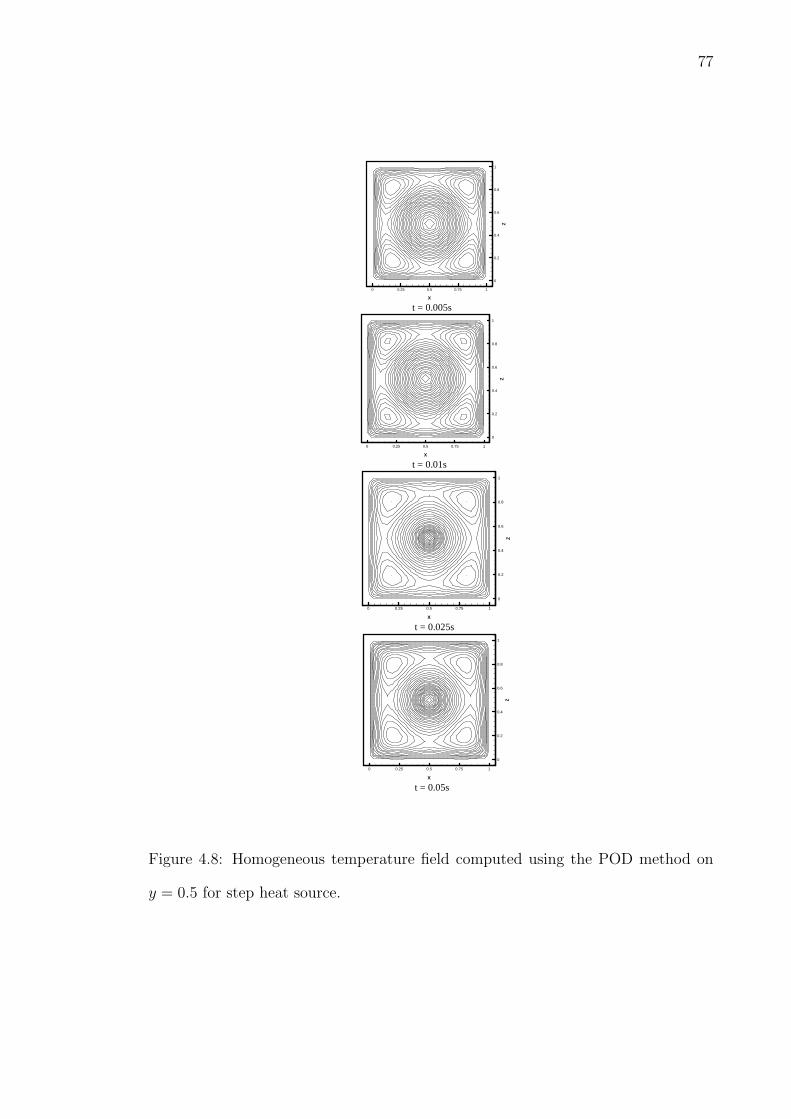
77
0 0.25 0.5 0.75 1
X
0
0.2
0.4
0.6
0.8
1
Z
t = 0.005s
0 0.25 0.5 0.75 1
X
0
0.2
0.4
0.6
0.8
1
Z
t = 0.01s
0 0.25 0.5 0.75 1
X
0
0.2
0.4
0.6
0.8
1
Z
t = 0.025s
0 0.25 0.5 0.75 1
X
0
0.2
0.4
0.6
0.8
1
Z
t = 0.05s
Figure 4.8: Homogeneous temperature field computed using the POD method on
y = 0.5 for step heat source.

78
0 0.01 0.02 0.03 0.04 0.05798
800
802
804
806
808
810
812
t (s)
T (
K)
Full−order model solutionReduced−order model solution
1 − (0.5,0.5,0.45)
2 − (0.5,0.5,0.4)
3 − (0.5,0.5,0.35)
Figure 4.9: Temperature evolution at thermocouple locations for step heat source.
thermocouple locations. For all following cases, the temperature is assumed to be
measured from t = 0 to t = 0.05s with a sampling interval δt = 0.001s, hence,
there are totally 150 measurements for each case. 26 basis functions are used in the
discretization of g(t) with equal step size of dt = 0.002s.
To obtain a good starting point for the MH sampling, an initialization step is first
conducted by running the sampling algorithm while solely increasing the likelihood.
A few hundred runs of this procedure is enough to provide a good initial guess of θ.
Fig. 4.10 plots the MAP estimates of the step heat source using MCMC samples
when σT takes different values. It is seen that the MAP estimates are stable to
various magnitudes of errors. In Fig. 4.11, the posterior mean estimate when
σT = 0.01 is plotted. The estimates are achieved using 10000 converged MCMC
samples. The upper and lower bounds plotted in the same figure are the values at
3 standard deviations from the sample mean, which is an indication of the highest
density region of the posterior state space. The σqj used in the proposal distribution
is 1% of the magnitude of θ(i)j . This is to guarantee that the proposal distribution
can fully explore the posterior state space while concentrating on the highest density

79
0 0.01 0.02 0.03 0.04 0.050
0.5
1
1.5
2
2.5
3
3.5
4
4.5x 10
5
t (s)g
(W
/m3)
True heat sourceMAP estimate when σ
T = 0.005
MAP estimate when σT = 0.01
MAP estimate when σT = 0.02
Figure 4.10: MAP estimates for the step heat source.
region. The regularization constant, λ is chosen to be 8.0e−9, 5.0e−9 and 2.0e−9,
respectively for the above three cases. The overall acceptance ratio for the chain
used in Fig. 4.11 is around 77.5%.
A triangular profile of heat source as shown in Fig. 4.12 is also reconstructed
following the same procedure as in the earlier example including using the POD
basis generated earlier with snapshots from the step heat source problem. Fig. 4.13
plots the MAP estimates of triangular heat source when σT has different values. It
is again seen that the estimates are relatively stable to the change of magnitude
of noise. Fig. 4.14 plots the posterior mean estimate when σT = 0.01. The same
proposal distribution as in the previous cases is used for this run. The overall
acceptance of the Markov chain is around 77.4%. It is seen that with simulated
noise, the posterior mean estimate approximates the true heat flux quite well.

80
0 0.01 0.02 0.03 0.04 0.050.5
1
1.5
2
2.5
3
3.5
4
4.5x 10⁵
t (s)
g(W
/m3)
True heat source
Posterior mean estimate
3 standard deviation bounds of the posterior distribution
Figure 4.11: Posterior mean estimate of the step heat source and probability bounds
of the posterior distribution when σT = 0.01.
o t
g(t)
0.02s 0.04s 0.05s
160kW/m3
80kW/m3
Figure 4.12: Profile of the triangular heat source.

81
0 0.01 0.02 0.03 0.04 0.05
0.6
0.7
0.8
0.9
1
1.1
1.2
1.3
1.4
1.5
1.6
1.7x 10
5
t (s)
g (
W/m
3)
True heat sourceMAP estimate when σ
T = 0.005
MAP estimate when σT = 0.01
MAP estimate when σT = 0.02
Figure 4.13: MAP estimates for the triangular heat source case.
0 0.01 0.02 0.03 0.04 0.05
0.6
0.8
1
1.2
1.4
1.6
x 105
t (s)
g (
W/m
3)
True heat sourcePosterior mean estimate3 standard deviation bounds of the posteriordistribution
Figure 4.14: Posterior mean estimate of the triangular heat source and probability
bounds of the posterior distribution when σ = 0.01.

82
4.6 Summary
In this chapter, an inverse radiation problem is solved using the Bayesian compu-
tational method. The posterior distribution of an unknown heat source strength
is computed from temperature measurements by modeling the measurement errors
as i.i.d. Gauss random variables. The Metropolis-Hastings algorithm was used to
explore the posterior state space and the POD method to reduce the computational
cost. The simulation results indicate that the method can provide accurate point
estimates of the unknown heat source as well as complete statistical information.
Although the study is devoted toward point heat source estimation, the method-
ologies can be extended to reconstruction of distributed heat sources as well. In
the situation where thermal properties are dependent on the temperature and large
temperature variation is observed, the Bayesian computation is still applicable.
In the model reduction used in the reconstruction of the step heat source in
the first example, for demonstration purposes the snapshots were generated using
the same heat source profile. While the snapshots generated with the step heat
source profile were capable resolving the triangular heat source profile in the second
example, they may not be appropriate for use in the identification of heat sources
of other profiles and a more comprehensive set of snapshots generated from various
heat source profiles will be needed. This is indeed an open important research area
of current interest.
In summary, it can be concluded in this chapter that by integrating POD
based reduced-order modeling in the likelihood computation, Bayesian computa-
tional method can be applied to complex nonlinear inverse continuum problems.
This is an demonstration of the generic applicability of Bayesian computational
method.

Chapter 5
Contamination source
identification in porous media flow
- Solving the PDEs backward in
time using Bayesian method
Bayesian computational method has been well addressed in the previous chapters for
inverse continuum problems of estimating physical parameters and dynamic bound-
ary conditions. In this chapter, the method is extended for another type of inverse
problem, the backward solution of PDE. A contamination source reconstruction
problem is studied herein to illustrate the methodology, in which an advection-
dispersion equation is solved backward in time. The plan of this chapter is as
follows. Section 5.1 introduces the mathematical definition of the problem. The
direct simulation of the contamination propagation is discussed in Section 5.2. It
is then followed by the hierarchical Bayesian formulation of the inverse computa-
tion. The posterior exploration algorithms are presented in Section 5.4. Section 5.5
83

84
contains numerical examples to demonstrate the developed methodology. Finally,
conclusions of the this work are summarized in Section 5.6.
5.1 Problem definition
The contamination source identification problem has received significant research
interest due to its applications in groundwater and soil cleanup. Addressing this
problem requires solving the governing partial differential equations (PDEs) of con-
taminant propagation in porous media flow backwards in time. Namely, the objec-
tive is to compute the history of contaminant concentration from current concentra-
tion data. The ill-posedness of this inverse problem and the difficulties in simulating
the contaminant propagation have been well-recognized. To facilitate the solution
to this challenging problem, a variety of methods have been developed over the past
several decades, which have been reviewed by Atmadja and Bagtzoglou [78] and
Michalak and Kitanidis [79].
The Bayesian approach was first introduced for solving contamination source
identification by Snodgrass and Kitanidis [80]. In follow up studies [48, 81], Micha-
lak and Kitanidis developed a confined Brownian motion model to enforce nonneg-
ativity of concentration estimates and techniques to select structure parameters of
the Bayesian posterior distribution. Ruppert et. al. [82, 83] have also developed
enhanced MCMC algorithms to improve the mixing of the sampling process from
the posterior distributions.
In contrast to the relatively straightforward formulation of the likelihood, mod-
eling the prior distribution in the Bayesian approach is more difficult. Considering
the structure of a spatially varying concentration field, the point-pair MRF model
is used. In this work, in addition to concentration fields, the standard deviation of

85
measurement errors and the scaling parameter of the prior distribution are treated
as random variables. These parameters are referred as ‘structure variables’ follow-
ing the terminology by Michalak and Kitanidis [48]. These parameters are often
called hyper-parameters as well. Hierarchical Bayesian analysis is used to derive the
joint distribution of structure parameters with the unknown concentration fields.
The joint posterior state space is then explored using a mixed sampler that samples
the concentration variables using the Gibbs algorithm and the structure parameters
using the MH algorithm.
Simulation data are used in this study to test the presented inverse computa-
tion method. The Darcy equation for porous media flow is first solved using the
global gradient post-processing method (Loula et al. [84]). The velocity field is then
used to solve the advection-dispersion equation of concentration using a streamline-
upwind/Petrov-Galerkin (SUPG) finite element method. All equations are solved
on a rather fine grid to generate simulation data, thus avoiding the so called ‘inverse
crimes’.
Propagation of contaminant in an impermeable porous medium can be described
by the following advection-dispersion equation (ADE) [85]:
φ∂c
∂t+∇ · (cu)−∇ · (D∇c) = cq, in Ω× (0, T ], (5.1)
with prescribed initial and (Neuman) boundary conditions,
c(x, 0) = c0(x), in Ω, (5.2)
D∇c · n = 0, on ∂Ω× (0, T ]. (5.3)
In the above equations, c is the concentration (mass fraction) of the contaminant and
c is the prescribed concentration values at the injection and production wells. Also
q denotes the volume flux rate at the wells and φ and D are the medium porosity

86
and dispersion tensor, respectively. Finally, Ω is the spatial domain and (0, T ] is the
total time span. The anisotropic dispersion coefficient D can be modeled as follows:
D = φαmI + ‖u‖[αlE(u) + αtE⊥(u)], (5.4)
with
E(u) =1
‖u‖u⊗ u, E⊥(u) = I− E(u), (5.5)
where I is the identity matrix, and αm, αl and αt are the molecular diffusivity,
longitudinal dispersion coefficient and transverse dispersion coefficient, respectively.
The Darcy velocity u can be computed from the following equations:
∇ · u = q, in Ω × (0, T ], (5.6)
u = −K(x)
µ(c)∇p, in Ω × (0, T ], (5.7)
u · n = 0, on ∂Ω × (0, T ], (5.8)
where p is the hydrodynamic pressure and K and µ are the permeability and dynamic
viscosity, respectively. In this study, we assume the variation of viscosity can be
neglected, i.e. that µ is a constant equal to the dynamic viscosity of the resident
fluid (water). Therefore, the ADE Eq. (5.1) is decoupled from the flow Eqs. (5.6)
and (5.7).
A direct (or forward) contaminant propagation problem is defined as the compu-
tation of the concentration distribution at all times t ∈ (0, T ], given initial condition
Eq. (5.2) and boundary condition Eq. (5.3). In the inverse problem of interest con-
sidered, the contamination concentration at current time t = T can be measured
at finite locations inside Ω. However, the history of contaminant distribution is not
known. Namely, c0 and the time span T between releasing time t = 0 of the conta-
minant and measurement time t = T are both unknown. The inverse problem is to

87
compute the concentration backwards in time, namely c(t) with t < T , on a finer
scale grid than the measurement scale grid. It is assumed that no prior knowledge
of releasing time and location of the contaminant is available. The releasing time is
defined as the time point corresponding to a backward computed concentration of
1.0 at any location.
5.2 The direct simulation and sensitivity analysis
5.2.1 Solution of the flow equations
The solution to the direct problem is required for the inverse computation. The
direct simulation can be separated into two parts: solution to the flow equations
and solution to the concentration equation. In the first part, the constant flow
velocity field is obtained by solving Eqs. (5.6) to (5.8). The velocity is then used in
solving Eqs. (5.1)-(5.5).
In the context of the finite element (FE) method, the most common approaches
to solving the flow Eqs. (5.6)-(5.8) are the stabilized finite element method, in which
the pressure and velocity are determined simultaneously, and the gradient post-
processing method, in which the pressure is found first and then the velocity is
calculated via gradient post-processing. The gradient post-processing method is
easier to implement and computationally less costly. It solves a diffusion equation
derived by substituting Eq. (5.7) into Eq. (5.6) for pressure first. The velocity is
then computed as the smoothed gradient of the pressure field. In this work, the flow
equations are solved using a global post-processing method as discussed in [84].
In the gradient post-processing approach, the pressure is solved using
∇(
K
µ∇p
)= −q, (5.9)

88
which is derived by substituting Eq. (5.7) into Eq. (5.6). The finite element technique
to solve this steady state diffusion equation is trivial. Once the pressure field is
obtained, Eq. (5.7) can be used to compute the velocity. However, since the finite
element solution of pressure is usually not smooth across element boundaries, the
velocity obtained by directly computing the gradient of pressure is discontinuous
across element boundaries, which is not physically feasible. To achieve a continuous
velocity solution, a global L2-smoothing post-processing problem is usually solved
with the following weak formulation:
(u,w) = (−K
µ∇p,w), (5.10)
where (·, ·) is the L2(Ω) inner product and w is the test function for velocity. Ac-
cording to Loula et al. [84], to further increase the accuracy of the post-processing
result, Eq. (5.10) is often modified:
(u,w) + (δh)α(∇ · u,∇ ·w) = (−K
µ∇p,w)
+(δh)α(q,∇ ·w), (5.11)
in which h is the finite element grid size. The parameters δ and α are here taken as
0.1 and 1, respectively [84]. Let
U = u|u ∈ (L2(Ω))dim,∇ · u ∈ L2(Ω),u · n = 0. (5.12)
The problem can be stated as to find u ∈ U , such that, for all w ∈ U , Eq. (5.11)
holds.
5.2.2 Solution of the concentration equation
After computing the velocity from the above approaches, one can return to Eq. (5.1)
to evaluate the concentration. To solve this advection-dispersion equation, the

89
SUPG finite element formulation is used [86]:
∫
Ωφ
∂c
∂twdΩ +
∫
Ω(u · ∇c)wdΩ +
∫
ΩqcwdΩ
+∫
ΩD∇c · ∇wdΩ +
nel∑
e=1
∫
Ωeτue∇w(φ
∂c
∂t+ ue · ∇c
+qc)dΩe =∫
ΩcqwdΩ +
nel∑
e=1
∫
Ωe
τue∇wcqdΩe. (5.13)
where w is the test function for concentration. The weak problem is to find c ∈H1(Ω) such that, for all w ∈ H1(Ω) Eq. (5.13) holds. The element based integrals
(the 5th term on the left hand side and the 2nd term on the right hand side) are
the SUPG stabilizing terms, in which τ is the upwind parameter. In this form,
the SUPG finite element formulation assumes the gradients of the test functions w
are discontinuous across the element boundaries. The stabilization parameter τ is
computed via the following formula:
τ =1
2
h
‖ue‖min(Pe
3, 1.0), (5.14)
where Pe is the local (element) Peclet number that is defined as:
Pe =1
2h‖ue‖3
uTe Due
. (5.15)
With the finite element formulations introduced above, the direct problem is
solved using two-dimensional bi-linear finite elements. The simulator was imple-
mented for parallel machines using PETSc [87] and has been tested by comparing
the results to solutions of various numerical examples documented in [86, 88, 89].
5.2.3 Sensitivity analysis
A discussion of sensitivity analysis is necessary to improve understanding of the
Bayesian formulation. To present the sensitivity analysis, a simpler inverse problem
90
is temporarily considered in this section. By assuming a known releasing time
of contaminant, the inverse problem introduced in Section 5.1 is reduced to the
estimation of a spatially varying function c0(x). This function estimation problem
is further transformed into a parameter estimation problem by the finite element
approximation:
c0(x) =m∑
j=1
θjfj(x), (5.16)
where fj(x)’s are the linear finite element basis functions and θj’s are the nodal
values of finite element approximation of c0 (fj instead of wj is used in this chapter
to avoid confusion with test functions in the weak formulations). The problem now
is to estimate an unknown m-dimensional vector θ with θ(j)=θj being the nodal
value associated with the jth basis function.
Let c(x, T ) be the concentration at measurement time t = T that is computed
from Eq. (5.1) using c0 as initial condition. Due to the linearity of the direct problem,
c(x, T ) =m∑
j=1
θjcj(x, T ) (5.17)
with cj(x, T ) being the direct solution of concentration at t = T using fj(x) as the
initial condition.
Let an N -dimensional vector Y denote the concentration measurement data at
t = T with Y (i) being the measurement at the ith sensor location (xi) and N being
the total number of sensors. Furthermore, let C be an N -dimensional vector with
C(i) = c(xi, T ). Using Eq. (5.17), C can be represented as:
C = Hθ, (5.18)
in which H is a N × m matrix with H(i, j) = cj(xi, T ). H is often called the
sensitivity matrix. It reflects the sensitivity of the concentration C(i) at each sensor
location i with respect to small variations in each parameter θ(j).

91
In the remaining part of this article, the following system relationship is assumed:
Y = Hθ + ω, (5.19)
where ω denotes the error between the measured data and the concentration com-
puted using the true initial condition. Therefore, ω contains both the random
measurement error and the numerical error. The objective of the simpler inverse
problem is to find an estimate of θ such that the discrepancy between Y and C is
minimized in some sense.
With the capability to simulate the direct problem and compute the sensitivity
matrix, we are now ready to investigate the Bayesian formulation.
5.3 Bayesian backward computation
5.3.1 Bayesian inverse formulation
If the random errors in Eq. (5.19) are assumed to be independent identically dis-
tributed (i.i.d.) Gauss random noise with zero mean and variance vT (standard
deviation σT =√
vT ), the likelihood can be formulated as:
p(Y |θ) =1
(2π)N/2vN/2T
exp−(Y −Hθ)T (Y −Hθ)
2vT
. (5.20)
It should be noticed that even though other distributions can be used to model
random errors, the Gaussian distribution is the most commonly used model. With
the likelihood Eq. (5.20) and prior distribution Eq. (3.12), the posterior can be
tentatively written as:
p(θ|Y ) ∝ exp−(Y −Hθ)T (Y −Hθ)
2vT
· exp(−1
2λθT Wθ). (5.21)
However, this posterior distribution depends on pre-fixed values of vT and λ. In
reality, the magnitude of the actual noise can only be roughly estimated. Selection

92
of λ is even more non-deterministic. Those two structure parameters are key to
the estimation of the posterior distribution and to the degree of smoothness of all
point estimates. Unlike earlier methods that try to select such structure parameters
before the inverse computation, the hierarchical Bayesian approach is considered
here to estimate the distribution of the structure parameters simultaneously with
the computation of the concentration distribution.
5.3.2 The hierarchical posterior distribution
The structure parameter is generally assumed to have a nearly non-informative
distribution over its support. For instance, in the current example, the structure
parameters λ and vT are both assumed a priori to be nearly uniformly distributed
over (0,∞]. However, the functional form of the nearly non-informative prior varies
for different structure parameters. In this study, conjugate priors [26] are used
to model the prior distribution of λ and vT . For Eq. (5.21), Gamma and inverse
Gamma distributions are chosen as priors for λ and vT , respectively:
p(λ) ∝ βα11
Γ(α1)λα1−1e−β1λ, λ ∈ (0,∞] (5.22)
p(v−1T ) ∝ βα2
2
Γ(α2)v−(α2+1)T e−β2v−1
T , vT ∈ (0,∞] (5.23)
A small value 1.0e − 3 is selected for the Gamma distribution constants α1, α2, β1
and β2. Thus, the distributions Eqs. (5.22) and (5.23) are nearly non-informative
over (0,∞].
With the hyper priors defined above, a hierarchical Bayesian posterior distribu-
tion can be computed as follows:
p(θ, λ, vT |Y ) ∝ p(Y |θ, vT )p(θ|λ)p(λ)p(vT )

93
∝ v−N/2T exp−(Y −Hθ)T (Y −Hθ)
2vT
· λm/2 exp−1
2λθT Wθ
·λα1−1 exp−β1λv−(1+α2)T exp−β2v
−1T , λ ∈ (0,∞] ∩ vT ∈ (0,∞]. (5.24)
5.3.3 The backward marching scheme
Equation (5.24) models the posterior distribution of the initial concentration field
when T is known. In the primary problem of interest in this study, T is an unknown
variable as well. Therefore, a backward marching scheme is used to reconstruct the
entire history of the concentration fields. The procedure is as follows.
1. Select a small time step ∆t.
2. Formulate a posterior in the form of Eq. (5.24) with T = ∆t.
3. Compute the posterior mean estimate of concentration at t = tcurrent − ∆t
(with tcurrent being the current time).
4. Continue marching backwards in time until the estimated concentration reaches
1.0 at any location, which is determined as the releasing time of the contami-
nant.
5. If t = 0 without the computed concentration reaching anywhere 1, set T =
T + ∆t and return to step 2.
In this approach, the concentration prior to the measurement time is recon-
structed backward in time until the releasing time is reached. Note that the sensi-
tivity problems only need to be solved once in this approach (solve the sensitivity
problem over a large time span and record concentration values at sensor locations
at all time steps).
Computing integrals of the hierarchical posterior distribution Eq. (5.24) is not a
trivial task. More importantly, one is often interested in the highest density region

94
of the posterior distribution. Based upon these considerations, a Gibbs sampling
based Markov chain Monte Carlo (MCMC) simulation method is used to compute
the posterior mean estimate of concentration.
5.4 Numerical exploration of the posterior distri-
bution
The MCMC sampler designed for exploring Eq. (5.24) is based on the basic MCMC
algorithm, the Metropolis-Hastings algorithm and the Gibbs algorithm. The pseudo-
code is the following:
Algorithm VI
1. Initialize θ(0), λ(0) and v(0)T
2. For i = 0 : Nmcmc− 1
— sample θ(i+1)1 ∼ p(θ1|θ(i+1)
−1 , λ(i), v(i)T , Y )
— sample θ(i+1)2 ∼ p(θ2|θ(i+1)
−2 , λ(i), v(i)T , Y )
—...
— sample θ(i+1)m ∼ p(θm|θ(i+1)
−m , λ(i), v(i)T , Y ).
— sample u ∼ U(0, 1)
— sample λ(∗) ∼ qλ(λ(∗)|λ(i))
— if u < A(λ(∗), λ(i))
λ(i+1) = λ(∗)
— else
λ(i+1) = λ(i),

95
— sample u ∼ U(0, 1)
— sample v(∗)T ∼ qv(v
(∗)T |v(i)
T )
— if u < A(v(∗)T , v
(i)T )
v(i+1)T = v
(∗)T
— else
v(i+1)T = v
(i)T .
In the above algorithm, Nmcmc is the total number of sampling steps, and
θ(i), λ(i), and v(i)T are the samples generated in the ith iteration for θ, λ, and vT ,
respectively. Also, θ(i)j is the jth component of θ(i). The notation θ
(i+1)−j denotes a
m − 1 dimensional vector θ(i+1)1 , ..., θ
(i+1)j−1 , θ
(i)j+1, ..., θ
(i)m . Also, p(·|θ(i+1)
−j , λ(i), v(i)T ) is
the full conditional distribution of θj in the ith iteration and u is a random number
generated from the standard uniform distribution U(0, 1). Finally, qλ(·|λ(i)) and
qv(·|v(i)T ) are the proposal distributions for λ and vT in the ith iteration, respectively.
The first part of this algorithm generates samples of θ using the Gibbs sampling
algorithm. It updates each component of θ a time from this component’s full condi-
tional distribution. In other words, the distribution of θj is conditional on all other
other random variables at current values, which are derived as follows:
p(θj|θ−j, λ, vT , Y ) ∼ N(µj, σ2j ), (5.25)
µj =bj
2aj
, σj =
√1
aj
(5.26)
aj =N∑
s=1
H2sj
vT
+ λWjj, bj = 2N∑
s=1
µsHsj
vT
− λµp, (5.27)
µs = Ys −∑
t 6=j
Hstθt, µp =∑
i6=j
Wijθi +∑
k 6=j
Wjkθk (5.28)
The acceptance probability of every Gibbs sample is 1; hence all the samples of θ
generated in this way are accepted.
96
The second part of this algorithm uses an MH sampler to update λ and vT . The
proposal distributions used to generate new samples of λ and vT are both normal
distributions as follows:
qλ(λ(∗)|λ(i)) ∼ N(λ(i), σ2
λ), (5.29)
and
qv(v(∗)T |v(i)
T ) ∼ N(v(i)T , σ2
v). (5.30)
There are two notes to this sampling process. First, the physical limits of θ are
0 and 1. However, if such limits are posed to the sampling process (i.e. rejecting
negative samples and samples greater than 1) the posterior mean estimate can never
reach the limits, which causes biasedness. Therefore, in this study, no constraint is
applied to the sampling process. By doing this, some physically unfeasible samples
are generated, but the posterior mean estimates are feasible. Second, design of the
proposal distributions qλ(λ(∗)|λ(i)) and qv(v
(∗)T |v(i)
T ) must ensure that the effective
regularization parameter (12λσ2) is not overly large.
5.5 Numerical examples
In this section, the above introduced methodology is demonstrated via three numer-
ical examples. Without loss of generality, the examples are studied in dimensionless
form.
5.5.1 Example 1: 1D advection-dispersion in homogeneous
media
The first example is a one-dimensional problem adopted from [78]. Inside the spatial
domain [0, 28], Eq. (5.1) holds with unit constant velocity, porosity and dispersion

97
0 5 10 15 20 25 30−0.02
0
0.02
0.04
0.06
0.08
0.1
0.12
0.14
xC
on
cen
tra
tion
, C
true concentrationposterior mean estimate
Figure 5.1: True and posterior mean estimate of concentration at t = 1.1.
0 5 10 15 20 25 30−0.02
0
0.02
0.04
0.06
0.08
0.1
0.12
x
Co
nce
ntr
atio
n,
C
true concentrationposterior mean estimate
Figure 5.2: True and posterior mean estimate of concentration at t = 1.9.
coefficient (u = 1.0, φ=1.0, D = 1.0). The concentration at x = 0 and x = 28 is
kept at zero. The initial concentration is a rectangular pulse:
c0(x) =
1, 13.5 ≤ x ≤ 14.5
0, 0 ≤ x ≤ 13.5, 14.5 ≤ x ≤ 28(5.31)
The concentration data are collected at t = 2.0, while the objective is to estimate
the concentration at t = 1.1 and t = 1.9.
Following [78], the direct problem is solved on a grid with 112 elements with
time step 0.02. The true and estimated concentration profiles at t = 1.1 and 1.9 are

98
1000 3000 5000 7000 90000.0000
0.0001
0.0002
0.0003
0.0004
0.0005
Figure 5.3: Posterior density of structure parameter λ in obtaining concentration
estimate at t = 1.1.
plotted in Figs. 5.1 and 5.2, respectively. The estimate at t = 1.1 is slightly better
because the regularization parameter is more optimal. This example is different
from the one in [78] in that (i) the concentration data are measured at 27 locations
instead of at all element nodes and (ii) random noise with magnitude of 5% of the
true concentration is added to the data. Still the estimates are quite accurate. The
posterior density of the structure parameter λ in obtaining concentration estimate
at t = 1.1 is plotted in Fig. 5.3 (Gamma distribution).
5.5.2 Example 2: 2D concentration reconstruction
In the following examples, we simulate a quarter area of the classical 5-spot problem.
A schematic of the problem is shown in Fig. 5.4. Inside the square domain (unit
side length), Eqs. (5.1) through (5.8) hold. The injection and production wells are
located at (0, 0) and (1, 1), respectively, both having volume flux rate q (varying in
different examples).
The actual initial concentration used to generate the simulation data has a nor-

99
u = 0 u = 0
v = 0
v = 0
qin
qout
0=∂∂
n
c0=
∂∂
n
c
Figure 5.4: Schematic of Example 2.
mal distribution peaked at (0.375, 0.75) with standard deviation 0.1. The direct
problem is solved on a 128× 128 finite element grid with a time step 0.02. Random
measurement errors are simulated from a normal distribution with zero mean and
standard deviation 0.005 (5% - 15% of the maximum recorded data in examples) in
the homogeneous cases and 0.002 in the heterogeneous case. The simulation con-
centration data are generated by adding random measurement errors to the direct
simulation solution at sensor locations. The data are used to recover the contami-
nant concentration history on a 64× 64 grid. The number of sensors used varies in
the following examples.
Diffusion-dominated transport in homogeneous porous media
In the first two-dimensional example, a diffusion-dominated mode is considered by
setting a very small value (q = 0.001) for the well flux rate. The permeability and
viscosity are both taken as 1.0. To ensure the molecular diffusion is the dominant
transport mechanism, φ, αm, αl, αt take values 0.1, 0.1, 0.01 and 0.001, respectively.
The concentration data are measured at t = T = 1.0 in this case. The sensors are
evenly distributed on nodes of an 8× 8 grid.

100
0
0.5
1
0
0.5
1x
0
0.5
1
y
0
0.5
1
0
0.5
1x
0
0.5
1
y
0
0.5
1
0
0.5
1x
0
0.5
1
y
0
0.5
1
0
0.5
1x
0
0.5
1
y
0
0.5
1
0
0.5
1x
0
0.5
1
y
0
0.5
1
0
0.5
1x
0
0.5
1
y
0
0.5
1
0
0.5
1x
0
0.5
1
y
0
0.5
1
0
0.5
1x
0
0.5
1
y
0
0.5
1
0
0.5
1x
0
0.5
1
y
0
0.5
1
0
0.5
1x
0
0.5
1
y
0
0.5
1
0
0.5
1x
0
0.5
1
y
0
0.5
1
0
0.5
1x
0
0.5
1
y
t=0
t=0.2
t=0.4
t=0.6
t=0.8
t=1.0(a) (b)
Figure 5.5: Reconstruction of the history of contaminant concentration: (a) The true
concentrations at different past time steps; (b) the reconstructed concentrations.
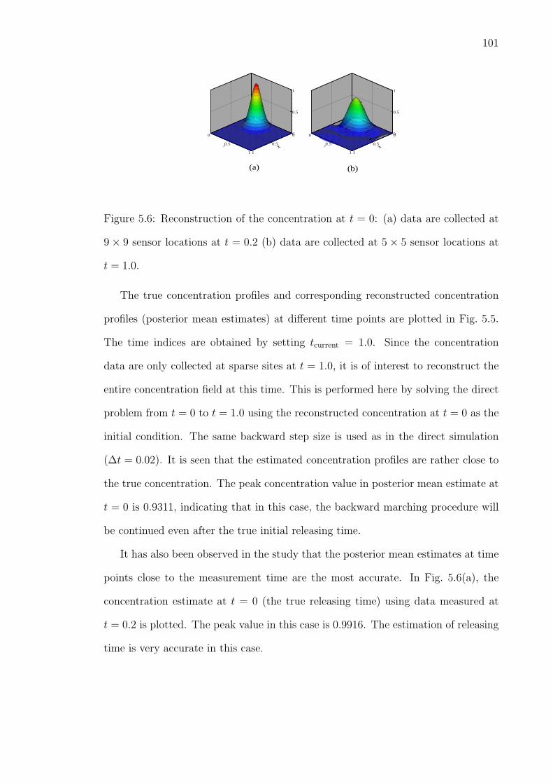
101
0
0.5
1
0
0.5
1x
0
0.5
1
y
0
0.5
1
0
0.5
1x
0
0.5
1
y
(a) (b)
Figure 5.6: Reconstruction of the concentration at t = 0: (a) data are collected at
9 × 9 sensor locations at t = 0.2 (b) data are collected at 5 × 5 sensor locations at
t = 1.0.
The true concentration profiles and corresponding reconstructed concentration
profiles (posterior mean estimates) at different time points are plotted in Fig. 5.5.
The time indices are obtained by setting tcurrent = 1.0. Since the concentration
data are only collected at sparse sites at t = 1.0, it is of interest to reconstruct the
entire concentration field at this time. This is performed here by solving the direct
problem from t = 0 to t = 1.0 using the reconstructed concentration at t = 0 as the
initial condition. The same backward step size is used as in the direct simulation
(∆t = 0.02). It is seen that the estimated concentration profiles are rather close to
the true concentration. The peak concentration value in posterior mean estimate at
t = 0 is 0.9311, indicating that in this case, the backward marching procedure will
be continued even after the true initial releasing time.
It has also been observed in the study that the posterior mean estimates at time
points close to the measurement time are the most accurate. In Fig. 5.6(a), the
concentration estimate at t = 0 (the true releasing time) using data measured at
t = 0.2 is plotted. The peak value in this case is 0.9916. The estimation of releasing
time is very accurate in this case.

102
To test if the number of sensors can be further reduced, the above estimation is
repeated to use data at t = 1.0 from a 5 × 5 sensor network. The posterior mean
estimate of the concentration at t = 0 (true releasing time) is plotted in Fig. 5.6(b).
The peak value is only 0.8 in this case. Therefore, although the peak location and
initial concentration profile can be identified in this case, the estimation of releasing
time is not acceptable.
Case I: Advection-dominated transport in homogeneous media
In the second numerical experiment, we reconsider the earlier example by changing
the following parameters: q = 0.04, αm = 0, αl = 0.04 and αt = 0.004. Convec-
tion and dispersion are the main mechanisms of contaminant propagation in this
case. Fig. 5.7 shows the true concentration profiles and posterior mean estimates
at different time points using data at t = T = 1.0. In this example, the data are
measured using a 16× 16 sensor network.
In Fig. 5.8, the estimated profile was generated using the data collected from
a 9 × 9 sensor network. It is seen that more fluctuations exist in the estimates.
However, the peak location and profile of concentration can still be resolved.
Case II: Advection-dispersion in heterogeneous media
In this example, we extend our earlier studies to heterogeneous porous media. All the
quantities remain the same as in Example 2 in Section 5.5.2 except the permeability,
which in this case is generated randomly from a joint log-normal distribution on a
32 × 32 finite lattice. The permeability mean at each site is 1.0 and the standard
deviation of log permeability is 1.5. An uncorrelated structure is assumed in this
case. The largest permeability and smallest permeability values in this example
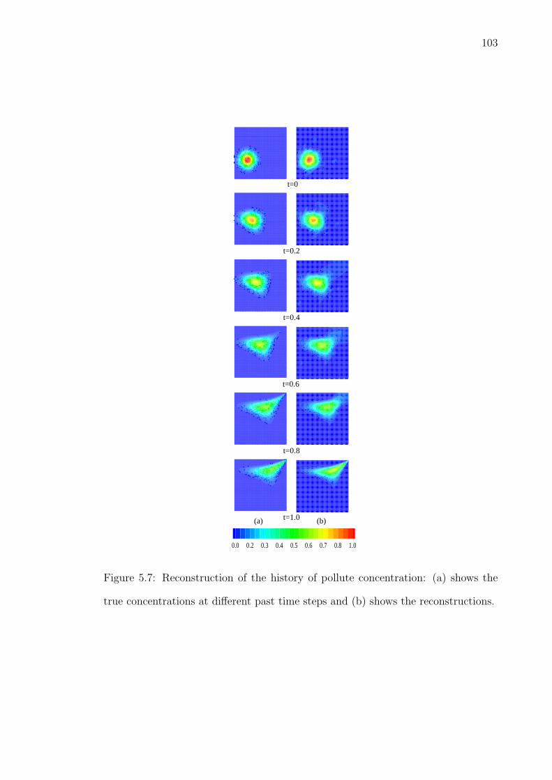
103
0.0 0.2 0.3 0.4 0.5 0.6 0.7 0.8 1.0
t=0
t=0.2
t=0.4
t=0.6
t=0.8
t=1.0(a) (b)
Figure 5.7: Reconstruction of the history of pollute concentration: (a) shows the
true concentrations at different past time steps and (b) shows the reconstructions.

104
0.0 0.2 0.3 0.4 0.5 0.6 0.7 0.8 1.0
t=0 t=0.2
t=0.4 t=0.6
t=0.8 t=1.0
Figure 5.8: Reconstruction of the contamination history when data are collected at
9× 9 sensor locations at t = 1.0.
differ by the magnitude of 105.
Fig. 5.9 shows the true concentration profiles and posterior mean estimates at
different time points using data at t = T = 1.0. In this example, the data are
measured from a 32 × 32 sensor network. The estimates obtained using data from
a 16 × 16 sensor network are also presented in Fig. 5.10. It is observed that the
estimates using less sensor data are comparable to the estimates in Fig. 5.9. Con-
sidering the heterogeneity and uniformly distributed sensor network, estimates in
Fig. 5.10 are quite impressive.
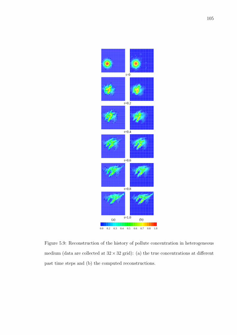
105
0.0 0.2 0.3 0.4 0.5 0.6 0.7 0.8 1.0
t=0
t=0.2
t=0.4
t=0.6
t=0.8
t=1.0(a) (b)
Figure 5.9: Reconstruction of the history of pollute concentration in heterogeneous
medium (data are collected at 32× 32 grid): (a) the true concentrations at different
past time steps and (b) the computed reconstructions.

106
0.0 0.2 0.3 0.4 0.5 0.6 0.7 0.8 1.0
t=0 t=0.2
t=0.4 t=0.6
t=0.8 t=1.0
Figure 5.10: Reconstruction of the history of pollute concentration in heterogeneous
medium (data are collected on a 16× 16 grid).
5.6 Summary
The hierarchical Bayesian computational method is extended in this chapter to solve
the contaminant history reconstruction problem in porous media flow. Through
this study, application of Bayesian method for backward solution of PDEs (initial
condition estimation) is demonstrated.
The regularity of the solution to this inverse problem is enforced by the Markov
Random Field model. Complete mathematical models including anisotropic dis-
persion and heterogeneous permeability are used in obtaining the direct simulation
results of contaminant propagation in porous media flow. The attributes of the

107
method are demonstrated via numerical examples in both homogeneous and hetero-
geneous porous media flows.
The current computational method successfully estimates instantaneously re-
leased contamination source in mixed fluids flow with constant viscosity. When
the mobility ratio of contaminant to resident fluid (water) deviates largely from
unity, a more complicated model is required to simulate the direct physical process.
However, the Bayesian method is still applicable in that scenario.

Chapter 6
Open-loop control of directional
solidification - A sequential
Bayesian computational
application
The Bayesian computational methods developed in chapter 3 and chapter 4 are
whole-time domain data inversion method. Namely, the unknowns at different time
points are modeled in the same joint posterior distribution conditional on all dy-
namic data. Such whole-time domain method is less practical than the sequential
estimation method when applied to real-time estimation-prediction applications.
For a dynamic system, it is advantageous to develop sequential Bayesian computa-
tional algorithms that can make real-time estimation conditional on dynamic data.
In this chapter, a directional solidification control problem is studied to demonstrate
the algorithm design of Bayesian filter for sequential solution to inverse problems.
The direct simulator of this study was developed by Ganapathysubramanian and
108

109
Zabaras in [101].
The real-time control of directional solidification is achieved by varying the ex-
ternal magnetic field gradient in this course of study, which is different from previous
solidification control mechanisms based on applying either a uniform or a rotating
magnetic field. The optimal magnetic gradient is estimated at each time step ac-
cording to the control objective, boundary data as well as magnetic gradient at the
previous time step. Random walk is used to model the evolution of magnetic gradi-
ent, which is treated as a random process in this approach. The likelihood is defined
in the way that the convection in the melt region is minimized. The posterior dis-
tribution of magnetic gradient at each time step is derived from the evolution prior
and the likelihood, from which the point estimates are computed. The Bayesian
control approach is analytically much simpler and computationally more affordable
than the previous whole-time domain control approach. It enables the on-line con-
trol of directional solidification. More significantly, it allows the quantification of
uncertainties in boundary conditions such as heat flux, and therefore, provides more
robust control solution.
The plan of this chapter is as follows. In Section 6.1, the physical problem is
defined. Section 6.2 introduces the fundamentals of Bayesian filter followed by the
sequential algorithm design for this particular control problem. Numerical examples
are provided in Section 6.3 to demonstrate the methodology. A brief summary is
finally provided in Section 6.4.

110
6.1 Open-loop control of directional solidification
using magnetic gradient
Solidification from the melt to near net shape is a commonly used manufacturing
technique. The fluid flow patterns in the melt affect the quality and properties of
the final product. For instance, solidification of alloys is invariably accompanied
by macrosegregation, which is caused by thermosolutal convection in the melt and
mushy zones. By controlling the flow behavior, the final solidified material can be
suitably affected. In this context, magnetic fields offer a promising means of control-
ling the solidification process. The effect of a Rotating Magnetic Field (RMF) on
crystal growth and solidification was investigated by Patzold et al. [90] and Roplekar
and Dantzig [91]. Galindo et al. [92] studied the effects of a rotating as well as a
travelling magnetic field on crystal growth processes. The use of a RMF results in
suppression of convection but fluctuations in temperature and concentration leading
to striation patterns in the crystal. Most of the magnetic field approaches to melt
flow control rely on the application of a constant magnetic field [93, 94]. A constant
magnetic field results in the Lorentz force that is used to damp and control the flow
[95, 96, 97, 98]. However, simultaneous application of a magnetic gradient results in
the Kelvin force along with the Lorentz force. This can be used for better control
of the melt flow resulting in higher crystal quality [99, 100].
In [101, 102], the effect of magnetic gradients on the quality of the crystal growth
is investigated. The infinite-dimensional functional optimization approach was taken
to compute optimal magnetic gradient history. This method requires the formulation
of an appropriate continuum adjoint problem that allows the analytical calculation
of the exact gradient of the objective functional. This whole-time domain approach

111
is very computationally expensive and requires storage of all transient temperature,
solute concentration and flow fields, which costs much computer memory. Thus,
this scheme is not applicable for real-time control of the solidification process.
In the following, a computational method for the open-loop control of the di-
rectional solidification is addressed using sequential Bayesian filter. The control
parameter is the time history of the imposed magnetic gradient. The objective
is to reduce the deviation of the velocity field in the melt region from conditions
corresponding to convection-less growth.
The direct solidification process is depicted in Fig. 6.1. Let Ω be a closed
bounded region in Rnsd , where nsd is the number of spatial dimensions, with a piece-
wise smooth boundary Γ. The region is filled with an incompressible, conducting
fluid. At time t = 0, a part of the boundary is cooled below the freezing temper-
ature of the fluid and solidification begins along that boundary. Two-dimensional
applications are considered in this study but the formulation presented is dimension-
independent. Let us denote the solid region by Ωs and the liquid region by Ωl. These
regions share a common solid-liquid interface boundary ΓI . As seen in Fig. 6.1, the
region Ωl has a boundary Γl which consists of ΓI (the solid-liquid interface), Γol (the
mold wall on the liquid side), Γbl (the bottom boundary of the liquid domain) and
Γtl (the top boundary of the liquid domain). Similarly Ωs has boundary Γs, which
consists of ΓI , Γos, Γbs and Γts. A time-varying magnetic field with spatial gradient
∂B∂z
is applied in the z direction.
The governing PDEs are:
in the melt region:
∇ · v = 0, (x, t) ∈ Ωl(t)× [0, tmax] (6.1)

112
ΓΓΓΓts ΓΓΓΓtl
BB
MELTMELTSOLIDSOLID
VVff
gg
ΓΓΓΓbs ΓΓΓΓbl
qosΓΓΓΓos qolΓΓΓΓI
x
z
ΓΓΓΓol
Figure 6.1: Schematic of the directional solidification system. A time-varying mag-
netic field with spatial gradient ∂B∂z
is applied in the z direction.
∂v
∂t+ v · ∇v = −∇p + Pr∇2v−RaT Prθleg + RaT Prγobθleg + RaCPrceg
+Ha2Prb2[−∇φ + v× eB]× eB, (x, t) ∈ Ωl(t)× [0, tmax] (6.2)
∂c
∂t+ v · ∇c = Le−1∇2c, (x, t) ∈ Ωl(t)× [0, tmax] (6.3)
∇2φ = ∇ · (v× eB), (x, t) ∈ Ωl(t)× [0, tmax] (6.4)
∂θl
∂t+ v · ∇θl = ∇2θl, (x, t) ∈ Ωl(t)× [0, tmax] (6.5)
∂θl
∂n= 0,
∂c
∂n= 0, (x, t) ∈ (Γl(t)− ΓI(t))× [0, tmax] (6.6)
v = 0,∂φ
∂n= 0, (x, t) ∈ Γl(t)× [0, tmax] (6.7)
v = 0, c = ci, θ = θi, x ∈ Ωl(t = 0) (6.8)
in the solid region:
∂θs
∂t= Rα∇2θs, (x, t) ∈ Ωs(t)× [0, tmax] (6.9)
θs = θ∗i , x ∈ Ωs(t = 0) (6.10)
∂θs
∂n= 0, (x, t) ∈ (Γs − Γos)× [0, tmax] (6.11)
θs = θs2, (x, t) ∈ Γos × [0, tmax] (6.12)
113
at the interface:
Rk∂θs
∂t− ∂θl
∂t= Ste−1vf · n, (x, t) ∈ ΓI(t)× [0, tmax] (6.13)
θ = θ0 + mc, (x, t) ∈ ΓI(t)× [0, tmax] (6.14)
∂c
∂n= Le(k − 1)(c + δ)vf · n, (x, t) ∈ ΓI(t)× [0, tmax] (6.15)
All of the above equations are non-dimensional with the following characteristic
scales: let L be a characteristic length of the domain; the characteristic scale for
time is taken as L2/α and for velocity as α/L; the dimensionless temperature θ is
defined as θ ≡ (T−To)/∆T where T , To and ∆T are the temperature, reference tem-
perature and reference temperature drop, respectively; likewise, the dimensionless
concentration field c is defined as (c − co)/∆c where c, co and ∆c are the concen-
tration, reference concentration and reference concentration drop, respectively; the
characteristic scale for the electric potential φ is taken as αBo where Bo is maxi-
mum value of the externally applied magnetic field. In these definitions, ρ is the
density, k is the thermal conductivity, α (α ≡ k/ρc) is the thermal diffusivity, D is
the solute diffusivity, σe is the electrical conductivity, and ν is the kinematic viscos-
ity. All fields and properties refer to the liquid domain unless denoted otherwise.
The magnitude of the applied gradient field is usually given as the value of ∇B2.
In this case, since B varies in the z direction only, it is given as B ∂B∂z
. Since only
dimensionless quantities will be used in the rest of this paper (unless is mentioned
otherwise), the symbol φ is used from now on to denote the dimensionless electric
potential.
To achieve a diffusion-based growth, the magnitude (b(t)) of the time-varying
magnetic field gradient must be chosen in such a way so as to negate the effects of
the thermal and convective buoyancy. In a whole-time domain approach, the control

114
objective is restated in terms of b(t) ∈ L2[0, tmax]. In particular, we are looking for
an optimal solution b(t) ∈ L2[0, tmax] such that:
S(b) ≤ S(b) ∀ b(t) ∈ L2[0, tmax], (6.16)
where
S(b) =1
2‖ v(x, t; b) ‖2
L2(Ωl×[0,tmax]) =1
2
∫ tmax
0
∫
Ωl(t)v(x, t; b) · v(x, t; b)dΩdt (6.17)
with the melt velocity v(x, t; b) defined from the solution of the direct problem
with b(t) as a function parameter. The main difficulty with the above optimization
problem is the calculation of the gradient S ′(b(t)) of the cost functional in L2[0, tmax].
Sensitivity and ajoint problems have to be solved, which requires storage of solution
to the direct problem at all time steps. Below, a Bayesian filter approach is presented
to allow real-time control of Eqs. (6.1) to (6.15) via estimating b(t). In the following
numerical studies, the direct problems (Eqs. (6.1) to (6.15)) are solved using a
single domain model along with volume-averaged governing transport equations is
used. Stabilized finite element techniques are used to discretize thermal, solutal and
momentum transport equations of the coupled system. Parallel iterative solution
techniques based on matrix free GMRES algorithm are employed for our numerical
simulations as well. These solver are developed by Ganapathysubramanian and
Zabaras in [101].
6.2 A Bayesian filter-based control approach
6.2.1 Bayesian filter
Bayesian filter refers to a group of predictor-corrector type sequential computation
algorithms [27]. The most commonly used Bayesian filters are the Kalman filter

115
)( 0Xp
evolution updating)|( 01 XXp
)( 1Xp
observation updating
)|( 11 DXp
evolution updating)|( 12 XXp
observation updating
)|( 12 DXp
)|( 22 DXp
)|( 11 XYp
)|( 22 XYp
.
.
.
Figure 6.2: Schematic of a Bayesian filter with Markov properties.
for linear dynamic system and the extended Kalman filter for nonlinear dynamic
system with explicit input-output relations. For a given dynamic system as
Xk+1 = Fk+1(Xk, Vk+1), (6.18)
Yk = Gk(Xk,Wk), (6.19)
where Xk and Yk are the state variable and measurement data at kth time step,
respectively, and Vk and Wk represent the associated process uncertainty and mea-
surement uncertainty, respectively, Bayesian filters compute conditional probability
p(Xk|Dk), (6.20)
where Dk stands for the ensemble of Y1, ..., Yk and p(X0|D0) = p(X0) is known.
The key steps to derive the posterior distribution 6.20 are the evolution updat-
ing and observation updating as shown in Fig. 6.2. The evolution updating for-

116
mulates distribution p(Xk+1|Dk with known models of p(Xk+1|Xk) and p(Xk|Dk).
p(Xk+1|Xk) is the conditional distribution of state parameter at the (k + 1)th time
step given parameter at the kth time step. This conditional distribution is subjected
to the model used in different applications. p(Xk|Dk) is the posterior distribution
of the parameter at kth time step, which contains all information regarding Xk at
time step k. After the evolution updating step, p(Xk+1|Dk actually provides the
prior distribution for estimation of Xk+1 at the (k + 1)th time step.
Observation updating is conducted when data at the (k + 1)th time step are
collected. It can be regarded as a standard Bayesian inference step. The poste-
rior distribution of p(Xk+1|Dk+1) is derived using the likelihood p(Yk+1|Xk+1) and
the prior p(Xk+1|Dk). It is necessary to point out that by using the scheme in
Fig. 6.2, the dynamic state parameter is assumed to be a Markov process, namely,
p(Xk+1|X0, ..., Xk) = p(Xk+1|Xk). The Markov property is also assumed for the
likelihood p(Yk|X0, ..., Xk) = p(Yk|Xk).
The essence of all Bayesian filters is the design of evolution updating step and
observation updating step. Once the posterior distribution p(Xk|Dk) is formulated
for all time steps, standard statistical computation algorithms can be used to explore
the posterior state space. For problems with low dimensionality, sequential MCMC
algorithms such as particle filter [38] are appropriate for the state space exploration
as well.
6.2.2 A sequential Bayesian controller for solidification con-
trol
For the solidification control problem, a random walk model is used for the state
parameter (magnitude of the magnetic gradient b(t) here). The Markov assumptions

117
on state parameter and likelihood apply to current problem as well. Let Bk be the
magnetic gradient value at the kth time step (b(k∆t) with ∆t being the time step
size), the random walk model is as follows:
Bk+1 = Bk + Vk+1, (6.21)
where Vk+1 is a Gauss random variable with zero mean and standard deviation σV .
Following this assumption, the evolution distribution can be written as:
p(Bk+1|Bk) ∝ 1
σV
exp−(Bk+1 −Bk)2
2σ2V
. (6.22)
The evolution updating is simplified to Eq. (6.22) for current problem. In another
word, the prior distribution of Bk+1 at each time step tk+1 is Eq. (6.22) with the
conditional value of Bk being the optimal estimate Bk in time step tk. This is because
the posterior distribution of Bk at each time step tk is implicit. The simplification
is also reasonable since for control purpose, only one magnetic gradient value that
is considered optimal should be applied at each time step.
To model the likelihood p(Yk|Bk), a few issues are addressed first. Firstly, the
observation data Yk in current problem are the desired values of physical quantities
to be controlled, for instance, to minimize the convection in melt part of the solid-
ification domain, zero velocity of the fluid is desired. Secondly, the system model
Gk(Bk,Wk) is implicit. It is a set of numerical simulators that solves the PDEs (6.1)
to (6.15) with optimal estimates of B0, ..., Bk−1 and guessed value of Bk. Thirdly,
Wk does not stand for measurement error in current problem. It represents the
uncertainties in the boundary conditions of above PDEs. For example, the fluctua-
tion of boundary heat flux for the energy equation. Based on these arguments, the
likelihood can be written as:
p(Yk|Bk, Wk) ∝ 1
σY
exp−(Yk −Gk(Bk,Wk)2
2σ2Y
. (6.23)

118
In above equation, σY is the standard deviation of a Gauss distribution. σY does not
correspond to variation of any physical data. It is solely a parameter for the control
of tradeoff between likelihood and prior in the optimization objective as illustrated
in the following discussion.
With the assumptions on prior and likelihood, the posterior distribution at the
(k + 1)th time step can be written as:
p(Bk+1,Wk+1|Dk+1) ∝ 1
σY
exp−(Yk+1 −Gk+1(Bk+1,Wk+1))2
2σ2Y
· 1
σV
exp−(Bk+1 −Bk)2
2σ2V
· 1
σW
exp−(Wk+1 − Wk+1)2
2σ2W
, (6.24)
in which the distribution of Wk+1 is assumed to be Gaussian with known mean value
Wk+1 and standard deviation σW .
As explained above, only one optimal value of Bk+1 need to be solved according to
the posterior distribution (6.24). Herein, this value is defined as the MAP estimate,
namely, the value of Bk+1 that maximizes the posterior probability in (6.24).
Bk+1, Wk+1 = argmaxBk+1,Wk+1
1
σY
exp−(Yk+1 −Gk+1(Bk+1,Wk+1))2
2σ2Y
· 1
σV
exp−(Bk+1 −Bk)2
2σ2V
· 1
σW
exp−(Wk+1 − Wk+1)2
2σ2W
, (6.25)
Since σY , σV and σW are all constants, maximizing (6.25) is equivalent to the min-
imizing of the following function:
Bk+1, Wk+1 = argminBk+1,Wk+1(Yk+1 −Gk+1(Bk+1,Wk+1))
2+
σ2Y
σ2V
· (Bk+1 −Bk)2 +
σ2Y
σ2W
· (Wk+1 − Wk+1)2, (6.26)
Solution to above optimization is feasible when the variation of heat flux is small.
However, instead of solving the optimal estimates of both Bk+1 and Wk+1, another
importance sampling approach is used to explore the uncertainty in Wk+1.

119
Since the distribution of Wk+1 is known in most applications. For example, the
boundary heat flux may vary around certain nominal value with variance estimated
from consecutive measurements. From the known Gaussian distribution of Wk+1,
a set of samples are drawn randomly at each time step. A weight that is propor-
tional to its probability is assigned to each sample. Let w(1)k+1, w
(2)k+1, ..., w
(n)k+1 be
the set of samples at time step tk+1 with n be the total number of samples and
f (1)k+1, f
(2)k+1, ..., f
(n)k+1 be the corresponding sample weights, the MAP estimator of
Bk+1 can be written as
Bk+1 = argminBk+1
n∑
i=1
f(i)k+1(Yk+1 −Gk+1(Bk+1, w
(i)k+1))
2+
σ2Y
σ2V
· (Bk+1 −Bk)2 (6.27)
Eq. (6.27) is a one variable optimization problem that can be solved using standard
gradient optimization method. It need to be pointed out that the ratio ofσ2
Y
σ2V, which
can be represented by a single parameter λ, controls the trade of between a flat
magnetic gradient and small convection.
Another approach to use importance sampling is to approximate the posterior
distribution of Bk+1 directly as:
p(Bk+1|Dk+1) ∝n∑
i=1
f(i)k+1[
1
σY
exp−(Yk+1 −Gk+1(Bk+1, w(i)k+1)
2
2σ2Y
· 1
σV
exp−(Bk+1 −Bk)2
2σ2V
], (6.28)
then define the MAP estimator using this distribution. This approach is not taken
here because the objective function become rather complex to optimizing.

120
Table 6.1: Specifications of the direct solidification problem.
Material specifications Setup specifications
27 NaCl aqueous solution Solidification in
Prandtl number 0.007 a rectangular cavity
Thermal Rayleigh number 200000 Dimensions 2cm x 2cm
Solutal Rayleigh number 10000 Fluid initially at 1 C
Lewis number 3000 Left wall kept at -25 w
Marangoni number 0
Stefan number 0.12778
Ratio of thermal diffusivites 1.25975
6.3 Examples
In this section, an example solidification process is studied to verify the methodology
developed above. The system specification and material properties are give in Table
6.1. Two cases are considered for this solidification process. In the first case, no
system uncertainty is considered, while in the second one, the boundary heat flux
has random variations. To demonstrate the effect of control mechanism applied to
the process, solidification without magnetic gradient control is first simulated. Two
snapshots are shown in Fig. 6.3. It can be seen that significant convection happens
in the melt region.
In the first three examples, no heat flux uncertainty is assumed. The examples
are the same except for value of λ. λ = 0.1, λ = 0.5 and λ = 1.0 are used for
these three examples, respectively. The computed optimal magnetic gradients as a
function of time are plotted in Figs. 6.4, 6.5 and 6.6, respectively. The corresponding

121
0 0.2 0.4 0.6 0.8 10
0.2
0.4
0.6
0.8
1
0 0.2 0.4 0.6 0.8 10
0.2
0.4
0.6
0.8
1
0 0.2 0.4 0.6 0.8 10
0.2
0.4
0.6
0.8
1
0 0.2 0.4 0.6 0.8 10
0.2
0.4
0.6
0.8
1
100 time step
200 time step
Figure 6.3: Snapshots of the solidification process without magnetic gradient control
applied. The left figures are the temperature fields and the right ones are the
streamlines.
time step
B(t
)
100 200 300 4000.95
0.96
0.97
0.98
0.99
1
1.01
1.02
1.03
Figure 6.4: Configuration of the optimal magnetic gradient when λ = 0.1.

122
time step
B(t
)
100 200 300 4000.96
0.97
0.98
0.99
1
1.01
1.02
Figure 6.5: Configuration of the optimal magnetic gradient when λ = 0.5.
time step
B(t
)
100 200 300 400-15
-10
-5
0
5
10
15
20
Figure 6.6: Configuration of the optimal magnetic gradient when λ = 1.
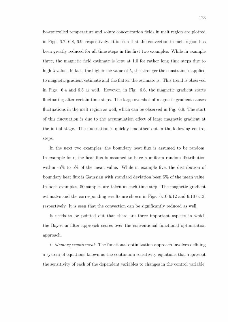
123
be-controlled temperature and solute concentration fields in melt region are plotted
in Figs. 6.7, 6.8, 6.9, respectively. It is seen that the convection in melt region has
been greatly reduced for all time steps in the first two examples. While in example
three, the magnetic field estimate is kept at 1.0 for rather long time steps due to
high λ value. In fact, the higher the value of λ, the stronger the constraint is applied
to magnetic gradient estimate and the flatter the estimate is. This trend is observed
in Figs. 6.4 and 6.5 as well. However, in Fig. 6.6, the magnetic gradient starts
fluctuating after certain time steps. The large overshot of magnetic gradient causes
fluctuations in the melt region as well, which can be observed in Fig. 6.9. The start
of this fluctuation is due to the accumulation effect of large magnetic gradient at
the initial stage. The fluctuation is quickly smoothed out in the following control
steps.
In the next two examples, the boundary heat flux is assumed to be random.
In example four, the heat flux is assumed to have a uniform random distribution
within -5% to 5% of the mean value. While in example five, the distribution of
boundary heat flux is Gaussian with standard deviation been 5% of the mean value.
In both examples, 50 samples are taken at each time step. The magnetic gradient
estimates and the corresponding results are shown in Figs. 6.10 6.12 and 6.10 6.13,
respectively. It is seen that the convection can be significantly reduced as well.
It needs to be pointed out that there are three important aspects in which
the Bayesian filter approach scores over the conventional functional optimization
approach.
i. Memory requirement: The functional optimization approach involves defining
a system of equations known as the continuum sensitivity equations that represent
the sensitivity of each of the dependent variables to changes in the control variable.

124
0 0.2 0.4 0.6 0.8 10
0.2
0.4
0.6
0.8
1
0 0.2 0.4 0.6 0.8 10
0.2
0.4
0.6
0.8
1
0 0.2 0.4 0.6 0.8 10
0.2
0.4
0.6
0.8
1
0 0.2 0.4 0.6 0.8 10
0.2
0.4
0.6
0.8
1
0 0.2 0.4 0.6 0.8 10
0.2
0.4
0.6
0.8
1
0 0.2 0.4 0.6 0.8 10
0.2
0.4
0.6
0.8
1
0 0.2 0.4 0.6 0.8 10
0.2
0.4
0.6
0.8
1
0 0.2 0.4 0.6 0.8 10
0.2
0.4
0.6
0.8
1
100 time step
200 time step
300 time step
400 time step
Figure 6.7: Snapshots of the solidification process with optimal magnetic gradient
applied when λ = 0.1. The left figures are the temperature fields and the right ones
are the streamlines.

125
0 0.2 0.4 0.6 0.8 10
0.2
0.4
0.6
0.8
1
0 0.2 0.4 0.6 0.8 10
0.2
0.4
0.6
0.8
1
0 0.2 0.4 0.6 0.8 10
0.2
0.4
0.6
0.8
1
0 0.2 0.4 0.6 0.8 10
0.2
0.4
0.6
0.8
1
0 0.2 0.4 0.6 0.8 10
0.2
0.4
0.6
0.8
1
0 0.2 0.4 0.6 0.8 10
0.2
0.4
0.6
0.8
1
0 0.2 0.4 0.6 0.8 10
0.2
0.4
0.6
0.8
1
0 0.2 0.4 0.6 0.8 10
0.2
0.4
0.6
0.8
1
100 time step
200 time step
300 time step
400 time step
Figure 6.8: Snapshots of the solidification process with optimal magnetic gradient
applied when λ = 0.5. The left figures are the temperature fields and the right ones
are the streamlines.

126
0 0.1 0.2 0.3 0.4 0.5 0.6 0.7 0.8 0.9 10
0.1
0.2
0.3
0.4
0.5
0.6
0.7
0.8
0.9
0 0.1 0.2 0.3 0.4 0.5 0.6 0.7 0.8 0.9 10
0.1
0.2
0.3
0.4
0.5
0.6
0.7
0.8
0.9
0 0.1 0.2 0.3 0.4 0.5 0.6 0.7 0.8 0.9 10
0.1
0.2
0.3
0.4
0.5
0.6
0.7
0.8
0.9
0 0.1 0.2 0.3 0.4 0.5 0.6 0.7 0.8 0.9 10
0.1
0.2
0.3
0.4
0.5
0.6
0.7
0.8
0.9
0 0.1 0.2 0.3 0.4 0.5 0.6 0.7 0.8 0.9 10
0.1
0.2
0.3
0.4
0.5
0.6
0.7
0.8
0.9
0 0.1 0.2 0.3 0.4 0.5 0.6 0.7 0.8 0.9 10
0.1
0.2
0.3
0.4
0.5
0.6
0.7
0.8
0.9
0 0.1 0.2 0.3 0.4 0.5 0.6 0.7 0.8 0.9 10
0.1
0.2
0.3
0.4
0.5
0.6
0.7
0.8
0.9
0 0.1 0.2 0.3 0.4 0.5 0.6 0.7 0.8 0.9 10
0.1
0.2
0.3
0.4
0.5
0.6
0.7
0.8
0.9
274 time step
322 time step
347 time step
400 time step
Figure 6.9: Snapshots of the solidification process with optimal magnetic gradient
applied when λ = 1. The left figures are the temperature fields and the right ones
are the streamlines.

127
time step
B(t
)
50 100 150
0.97
0.975
0.98
0.985
0.99
0.995
1
Figure 6.10: Configuration of the optimal magnetic gradient when the boundary
heat flux has random fluctuation with a uniform distribution.
time step
B(t
)
50 100 150
0.97
0.975
0.98
0.985
0.99
0.995
1
Figure 6.11: Configuration of the optimal magnetic gradient when the boundary
heat flux has random fluctuation with a Gaussian distribution.

128
0 0.2 0.4 0.6 0.8 10
0.1
0.2
0.3
0.4
0.5
0.6
0.7
0.8
0.9
1
0 0.2 0.4 0.6 0.8 10
0.1
0.2
0.3
0.4
0.5
0.6
0.7
0.8
0.9
1
0 0.2 0.4 0.6 0.8 10
0.1
0.2
0.3
0.4
0.5
0.6
0.7
0.8
0.9
1
0 0.2 0.4 0.6 0.8 10
0.1
0.2
0.3
0.4
0.5
0.6
0.7
0.8
0.9
1
0 0.2 0.4 0.6 0.8 10
0.1
0.2
0.3
0.4
0.5
0.6
0.7
0.8
0.9
1
0 0.2 0.4 0.6 0.8 10
0.1
0.2
0.3
0.4
0.5
0.6
0.7
0.8
0.9
1
0 0.2 0.4 0.6 0.8 10
0.1
0.2
0.3
0.4
0.5
0.6
0.7
0.8
0.9
1
0 0.2 0.4 0.6 0.8 10
0.1
0.2
0.3
0.4
0.5
0.6
0.7
0.8
0.9
1
50 time step
100 time step
150 time step
200 time step
Figure 6.12: Snapshots of the solidification process with optimal magnetic gradi-
ent applied when the boundary heat flux has random fluctuation with a uniform
distribution. The left figures are the temperature fields and the right ones are the
streamlines.
129
0 0.2 0.4 0.6 0.8 10
0.1
0.2
0.3
0.4
0.5
0.6
0.7
0.8
0.9
1
0 0.2 0.4 0.6 0.8 10
0.1
0.2
0.3
0.4
0.5
0.6
0.7
0.8
0.9
1
0 0.2 0.4 0.6 0.8 10
0.1
0.2
0.3
0.4
0.5
0.6
0.7
0.8
0.9
1
0 0.2 0.4 0.6 0.8 10
0.1
0.2
0.3
0.4
0.5
0.6
0.7
0.8
0.9
1
0 0.2 0.4 0.6 0.8 10
0.1
0.2
0.3
0.4
0.5
0.6
0.7
0.8
0.9
1
0 0.2 0.4 0.6 0.8 10
0.1
0.2
0.3
0.4
0.5
0.6
0.7
0.8
0.9
1
0 0.2 0.4 0.6 0.8 10
0.1
0.2
0.3
0.4
0.5
0.6
0.7
0.8
0.9
1
0 0.2 0.4 0.6 0.8 10
0.1
0.2
0.3
0.4
0.5
0.6
0.7
0.8
0.9
1
50 time step
100 time step
150 time step
200 time step
Figure 6.13: Snapshots of the solidification process with optimal magnetic gradi-
ent applied when the boundary heat flux has random fluctuation with a Gaussian
distribution. The left figures are the temperature fields and the right ones are the
streamlines.

130
Using these equations, a functional form for the gradient of the cost functional
is evaluated in terms of a new set of partial differential equations. This set of
equations is called the continuum adjoint equations. At each optimization step
the direct problem is solved for the whole time history. Then using this data the
adjoint equations are solved backwards in time. The gradient of the cost functional
is evaluated using the adjoint variables. The sensitivity equations are solved to
estimate the step size in the descent direction of the optimization routine. During
this process, the whole direct problem solution has to be stored in memory for later
use in the solution of the adjoint equations. This is enormously memory intensive.
In the solidification example considered, the temperature, velocity (2 values u ,v),
pressure, concentration and potential have to be stored at all the grid points for
all the time steps (3500 points for 400 timesteps). The memory requirement is
to store 6x3500x400 variables which easily goes over 300 MB. For problems with
finer resolution and larger time histories, the memory requirements quickly become
unmanageable. While in the Bayesian approach, only the direct simulation result at
previous one time step is stored. As the example problem considered, the memory
storage is on the order of 10−3 of the one in the conventional approach.
ii. Model complexity: Three sets of equations have to be solved in the conven-
tional approach. The direct problem is a nonlinear problem that has to be solved
over the whole time domain. The adjoint problem is a linear problem that is solved
backwards in time. At each time step, the direct solution is accessed and the direct
variables corresponding to that time step are used in the solution of the adjoint vari-
ables. The sensitivity equations are then solved for the whole time domain. While
in the Bayesian approach, only the direct problem is solved and in each time step,
the direct problem only needs to be solved one time step further.
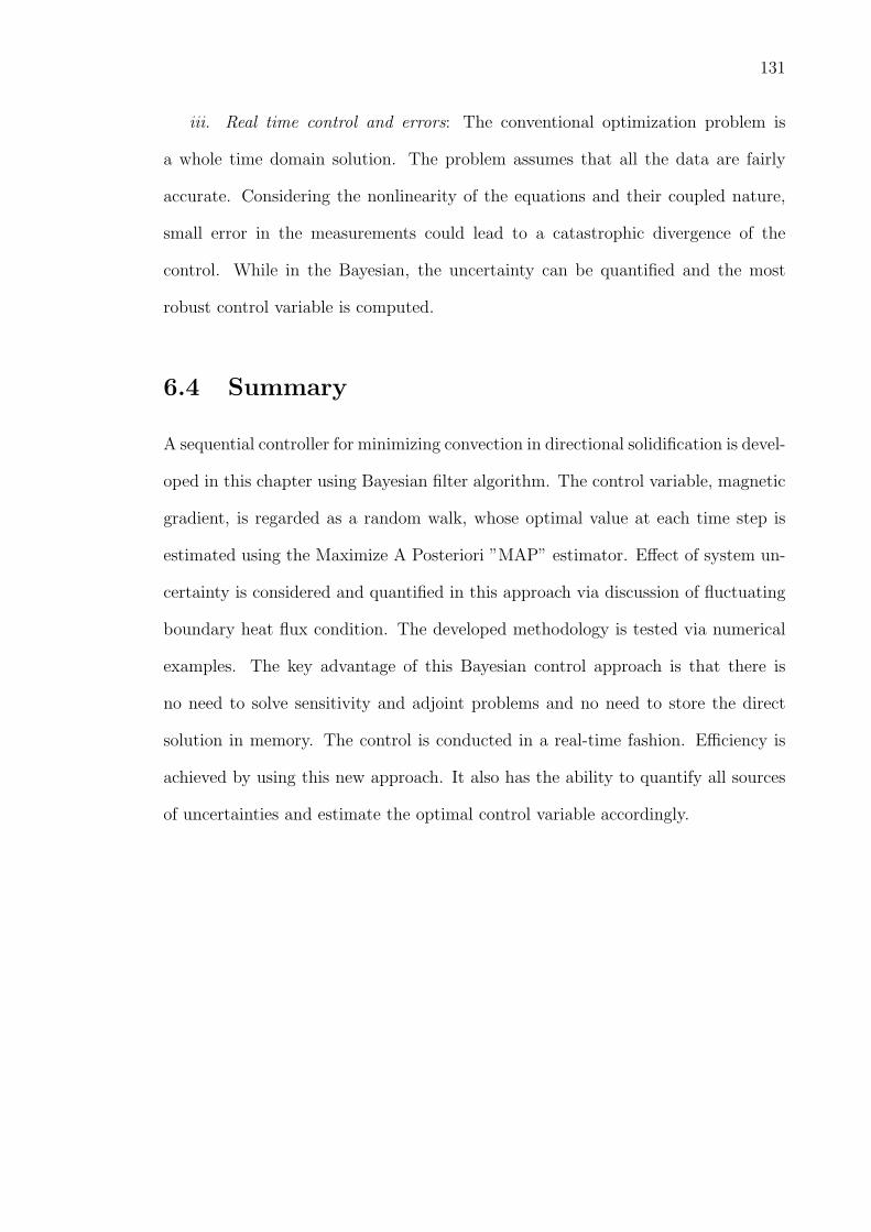
131
iii. Real time control and errors: The conventional optimization problem is
a whole time domain solution. The problem assumes that all the data are fairly
accurate. Considering the nonlinearity of the equations and their coupled nature,
small error in the measurements could lead to a catastrophic divergence of the
control. While in the Bayesian, the uncertainty can be quantified and the most
robust control variable is computed.
6.4 Summary
A sequential controller for minimizing convection in directional solidification is devel-
oped in this chapter using Bayesian filter algorithm. The control variable, magnetic
gradient, is regarded as a random walk, whose optimal value at each time step is
estimated using the Maximize A Posteriori ”MAP” estimator. Effect of system un-
certainty is considered and quantified in this approach via discussion of fluctuating
boundary heat flux condition. The developed methodology is tested via numerical
examples. The key advantage of this Bayesian control approach is that there is
no need to solve sensitivity and adjoint problems and no need to store the direct
solution in memory. The control is conducted in a real-time fashion. Efficiency is
achieved by using this new approach. It also has the ability to quantify all sources
of uncertainties and estimate the optimal control variable accordingly.

Chapter 7
Multiscale permeability estimation
in heterogeneous porous media - A
multiscale Bayesian inversion
method
A multiscale Bayesian inversion method based on the hierarchical Markov tree
(HMT) model [103, 104] is presented in this chapter to address heterogeneous pa-
rameter estimation at different length scales. The methodology is introduced using
permeability estimation in heterogeneous porous media as the prototype problem.
The study is composed by two parts. In the first part, the permeability is esti-
mated at one length scale that is finer than the data-collection scale using Markov
Random Field as the prior. This method performs well for regular (smooth) per-
meability fields as tested by an example of estimating a permeability field whose
logarithm is bilinear. In the second part, the more generic case of a permeability
with random discontinuities is considered. A two-layer HMT model is used to model
132

133
the random permeability at both the data-collection scale and at another much finer
scale. The hierarchical Bayesian analysis is used to derive the posterior distribu-
tions of the permeability at both scales. The inner-scale spatial correlation of the
random permeability is assumed as a Markov chain. A hybrid MCMC algorithm is
developed to explore the posterior distributions of the permeability. In Section 7.1,
the permeability estimation problem is defined and the direct mathematical model
is introduced. In Section 7.2, the Bayesian formulations of the above discussed two
cases are derived and the associated MCMC algorithms are presented. Section 7.3
contains the numerical examples that are used to demonstrate the methodologies
developed in Section 7.2. A brief summary is provided in Section 7.4.
7.1 Problem definition
Simulation of transport processes in porous media flow requires the permeability
of the medium as an input. Nevertheless, the permeability of most media such
as the one of a geo-engineering system is usually not directly attainable and must
be estimated from related well or seismic data [51, 105]. The two types of well
data available are the static well data, which are the permeability measurements of
sample porous structures at the wells, and the dynamic well data, which are the
flow measurements at wells. The estimates obtained using static data are local,
therefore, are not able to represent the distributed porous structure. In this study,
we use dynamic flow data to compute the permeability, which makes permeability
estimation an inverse problem. A complication of this inverse problem is that the
well data are expensive to obtain and can only be collected at sparse locations. The
permeability in practice may vary significantly in space with random discontinuities.
To address this strongly ill-posed inverse problem, the direct mathematical model

134
is introduced first.
In this study, we consider the same direct model as in Chapter 5 for species
transport in porous media flow,
∇ · u = q, in Ω × (0, T ], (7.1)
u = −K(x)
µ(c)∇p, in Ω × (0, T ], (7.2)
φ∂c
∂t+∇ · (cu)−∇ · (D∇c) = cq, in Ω× (0, T ], (7.3)
with,
u · n = 0, on ∂Ω, × (0, T ], (7.4)
D∇c · n = 0, on ∂Ω× (0, T ]. (7.5)
c(x, 0) = c0(x), in Ω. (7.6)
with all the parameters defined in Chapter 5.
injection well
production well
u = 0
0=∂∂
n
cu = 0
0=∂∂
n
c
v = 0 0=∂∂
n
c
v = 0 0=∂∂
n
c
Figure 7.1: Schematic of a 9-spot problem. A injection well is located at the center
of the domain and 8 production wells distribute at the rest nodes of a 2× 2 grid. In
general, for a n-spot problem, the n wells distribute at nodes of a (√
n−1)×(√
n−1)
grid with the single injection well at the center.
The permeability K(x) is unknown in the above equations and will be estimated
from dynamic well data (pressure and/or concentration at wells in this study). In

135
specific, we consider a n-spot problem inside a square domain. An injection well is
located at the center of the square domain, while n-1 production wells distribute at
the rest nodes of a (√
n − 1) × (√
n − 1) grid. For instance, for a 9-spot problem,
the well distribution is as shown in Fig. 7.1. Pressure and concentration data are
measured at these well locations and used to estimate the permeability K(x). The
solution method to the direct problem has been introduced in Chapter 5 and the
same direct simulator will be used in this study with the permeability being the
input to the simulator and pressure and concentration data at the wells being the
output. As the inverse problem is concerned, we are interested in computing the
permeability at length scales that are equal or finer than the data-collection scale
((√
n− 1)× (√
n− 1)).
7.2 Bayesian posterior distribution of the random
permeability
The inverse problem can be posed in two different ways. In the first case, there
is a fixed target length scale on which the permeability is needed. This length
scale can be much smaller than the characteristic length scale of the sensor network
(here, the smallest distance between two wells). Solution to this strongly ill-posed
inverse problem is possible by introducing prior distribution model such as MRF.
This approach can be shown to provide satisfactory results when the underlying
permeability has good regularity (smoothness). In the second and more general
case, the permeability is expected to have random discontinuities. The problem
becomes more complicated and the smoothing prior model MRF will not be able to
resolve the rich heterogeneous feature of the porous structure. A potential approach

136
in this case is to estimate the permeability at different length scales by having
a hierarchically structured prior distribution. In the following sections, Bayesian
formulations for these two different situations are presented.
7.2.1 Formulation I: MRF-based one scale model
In this case, the objective is to estimate the permeability on a pre-determined length
scale that is finer than the data-collection scale. Let Y denote the concentration
measurements at the n-1 production wells (concentration at the injection well is
treated as a known boundary condition). The system model can be denoted as:
Y = F (K(x)) + ω, (7.7)
where F (K(x)) is the simulator that solves Eqs. (7.1) to (7.6) with K(x) being the
input and concentration at production wells as the output, and ω is the random
measurement noise following a zero mean Gaussian distribution.
To parameterize the permeability, the square domain is divided into a MxM
lattice with M being the number of elements in each coordinate and m = M ×M
being the total number of elements (pixels). Note that here m is much larger than
n. The permeability is assumed to be uniform within each pixel. Let θ denote the
unknown vector containing logarithms of the permeability values at all these pixels
(the dimension of θ is m). The system equation can be rewritten as:
Y = F (θ) + ω. (7.8)
The reason for representing the permeability using the local uniform model is that
permeability, by its definition, is a locally averaged parameter that models the pro-
portionality relation between the pressure gradient and the velocity field. Also note
that in this work θ is taken as the logarithm of the permeability value. This is

137
because the permeability is often assumed to be log-normal to account for its non-
negativity, and its logarithm follows Gaussian distribution, for which it is easier to
model the priors.
With the above assumptions, the posterior distribution of log permeability vector
θ is:
p(θ|Y ) ∝ exp− 1
2σ2[F (θ)− Y ]T [F (θ)− Y ] · exp−1
2λθT Wθ, (7.9)
in which σ is the standard deviation of the measurement error and W is defined in
the previous MRF model (Section 2.3). This formulation is identical as the inverse
formulations in the previous chapters. However, the exploration of it is much more
difficult because the dimension of θ is in general large and the direct simulation is
costly. The hybrid MCMC algorithm used to solve this issue is discussed in Section
7.2.3. It is emphasized here again that the formulation in Eq. (7.9) is only able
to provide smooth permeability estimate on fine grid with sparse well data. It will
be shown that it works well for applications where only the averaged equivalent
permeability is required.
7.2.2 Formulation II: HMT-based two scale model
In the more general case, the permeability has many random discontinuities that
have magnitudes varying over several length scales. For example, the logarithm of
a random permeability is shown in Fig. 7.2. Inside the [0, 8]× [0.8] square domain,
there are two sub-areas with large-magnitude permeability ([2, 4]× [4, 6] and [4, 6]×[2, 4]). The permeability in the upper-left darker area ([2, 4]× [4, 6]) has magnitude
around 3,000. The permeability in the lower-right darker area ([4, 6] × [2, 4]) is
around 700. While the permeability in the remaining of the domain is 1.0. Within
each sub-area with large permeability, the logarithm of permeability is a random

138
0 2 4 6 80
1
2
3
4
5
6
7
8
1
2
3
4
5
6
7
8
Figure 7.2: The log permeability of a random porous medium. Two large magni-
tude discontinuities occur within two darker areas ([2, 4] × [4, 6] and [4, 6] × [2, 4]).
Within each of these areas, the permeability is a correlated Gaussian random field
with a correlation function of ρ(r) = e−r2with r being the spatial distance among
two locations. The random variations within each darker area have much smaller
magnitude than the average magnitudes of both darker areas permeability.
2 2.5 3 3.5 44
4.2
4.4
4.6
4.8
5
5.2
5.4
5.6
5.8
6
7.8
7.9
8
8.1
8.2
8.3
Figure 7.3: The enlarged upper-left darker area ([2, 4]×[4, 6]) of the log permeability
in Fig. 7.2.

139
4 4.5 5 5.5 62
2.2
2.4
2.6
2.8
3
3.2
3.4
3.6
3.8
4
6.2
6.3
6.4
6.5
6.6
6.7
6.8
Figure 7.4: The enlarged lower-right darker area ([4, 6]× [2, 4]) of log permeability
in Fig. 7.2.
Gaussian field with a correlation function of ρ(r) = e−r2with r being the distance
between two locations. These two random fields are zoomed in as shown in Fig
7.3 and Fig. 7.4, respectively. It is obvious that the Bayesian formulation given in
Section 7.2.1 will not work for estimating such permeability since it tends to smooth
the field.
We consider a hierarchical representation of the heterogeneous permeability in
this section as depicted in Fig. 7.5 [103]. At the coarsest scale (a lumped parameter
representation), a homogeneous value is used to approximate the permeability, which
is represented as the root pixel in Fig. 7.5. Assuming that in each subsequent smaller
length scale, every pixel (parent) is split into t different pixels (children) as indicated
in Fig. 7.5, where t is equal to 4 (of course, t can take other values as well). As the
splitting proceeds, finer and finer description of the permeability is allowed.
For convenience of discussion, we introduce the following notation. Let s be
the scale index, or say the distance of the scale to the root pixel (s=0 for the root
scale), ms be the number of pixels in the sth layer, obviously ms = ts, and θsi be the
logarithm of permeability value at the ith pixel of the sth layer. In addition, we use

140
s = 0 (root scale)
s = 1 (1st scale)
s = 2 (2nd scale)
Figure 7.5: A scheme of hierarchical Markov tree model.
Θs to denote all pixel values (log permeability values) at the sth scale. Finally, we
assume Y s is the data set at the sth level.
As the inverse problem considered in this section, one computes the posterior
distribution p(Θs|Y r)’s for all s that is equal to or larger than r. To derive these
posterior probabilities, the hierarchical Markov tree model shown with a graphic
representation in Figure 7.5 is used.
The situation where the permeability is to be estimated on two length scales r
and s is first considered. r is the data-collection scale and s > r is a scale that has
much higher resolution than r. It is also assumed that each pixel on scale r is split
into t pixels on length scale s. The Bayesian formulation for this inverse problem is
composed by two parts as discussed next.
To estimate the permeability on scale r, no prior regularization is needed since it
is the same length scale as the data-collection scale. The given information of well
data is enough to solve the problem. Therefore, the distribution of permeability on
length scale r is modeled using the likelihood only.
p(Θr|Y r) ∝ exp− 1
2σ2[F (Θr)− Y r]T [F (Θr)− Y r], (7.10)
which implies that the prior of Θr is uniform.

141
The next step is to derive the posterior distribution of Θs, the log permeability
estimate on length scale s. Using the hierarchical Bayesian analysis, it is easy to
obtain that
p(Θs, Θr|Y r) ∝ p(Y r|Θs, Θr)p(Θs, Θr) ∝ p(Y r|Θs)p(Θs|Θr)p(Θr). (7.11)
In the derivation of Eq. (7.11), we assume that the data do not depend on coarser
scale permeability once the finer scale permeability is known. This is valid since the
finer scale permeability contains more information of the porous structure than the
coarser scale permeability. The coarser scale log permeability Θr in this formulation
is actually treated as the hyper-parameter and only matters in the prior distribution
of finer scale permeability Θs.
The likelihood in Eq. (7.11) is the same as Eq. (7.10) by replacing Θr with
Θs. The hyper-prior distribution p(Θr) in Eq. (7.11) is nothing but Eq. (7.10). To
model the conditional prior distribution p(Θs|Θr), the Markov assumption is used
for both the cross-length-scale and the inner-length-scale correlations. Namely,
p(θsi |Θs
−i, Θr) ∝ p(θs
i |θs∼i, θ
rpi
), (7.12)
where Θs−i denotes the vector θs
1, ..., θsi−1, θ
si+1, ..., θ
sms, θs
∼i denotes the permeabil-
ity pixels adjacent to θsi in the same scale (4 of them in 2-dimension case), and θr
pi
denotes the parent pixel of θsi on the length scale r. Eq. (7.12) states that the
distribution of permeability at a pixel on the finer scale depends only on the per-
meability at adjacent sites and the parent permeability at the coarser length scale.
This conditional distribution also defines a valid joint prior distribution of Θs condi-
tional on Θr by Hammerseley-Clifford theorem [37]. Since the sampling algorithms
introduced in the next section only require the conditional distribution to explore
the posterior state space, the joint distribution formula corresponding to Eq. (7.12)

142
is not needed.
Although examples in this chapter only involve estimation of the permeability on
two length scales, there is an interest to derive the Bayesian formula for estimating
permeability at arbitrary number of length scales. The downward Markov property
is assumed in this regard. Namely,
p(Θs|Θs−1, Θs−2, ..., Θ0) ∝ p(Θs|Θs−1), (7.13)
which is a perfectly admissible assumption since the finer scale permeability repre-
sentation contains all information about the permeability resolution at the coarser
scales. With this assumption, the posterior of permeability on S ordered length
scales s1, s2, ..., sS, with s1 being the coarsest and also the data-collection scale, is
p(Θs1 , ..., ΘsS |Y s1) ∝ p(Y s1|ΘsS)p(ΘsS |ΘsS−1)...p(Θs2|Θs1)p(Θs1). (7.14)
The conditional distributions p(Θsi|Θsi−1) in the above equation can be derived as
in Eq. (7.12), the likelihood has the same form as Eq. (7.10), and the hyper-prior
p(Θs1) is basically its likelihood.
7.2.3 Exploring the posterior state space
The Bayesian posterior distributions derived in the previous two sections both have
very high-dimension in general. The single component updating schemes used in
previous chapters are too expensive to implement for these formulations, while the
acceptance ratio will be extremely low if the unknown log permeability field is
updated entirely in each MCMC sampling step. To explore the joint state space
efficiently, the block hybrid MCMC sampler is used here [38]. The procedure of
this design is to first divide the 2-dimensional permeability field (Ms × Ms pixels

143
* *
** *** ......
* *
** *** ......
* *
** *** ......
Figure 7.6: Schematics of single component updating (upper-left), block updating
(upper-right), and whole field updating (lower).
on each length scale s) into certain equal-sized blocks. The pixel values inside the
same block are updated the same time at one sampling iteration.
A schematic comparing the single component, the entire field, and the block
updating methods is shown in Fig. 7.6. In the block hybrid MCMC, the log per-
meability on pixels inside each block is updated in one MCMC step. The candidate
sample vector for these parameters inside each block is generated one component
at a time using the conditional distribution Eq. (7.12) as the proposal distribution.
In this algorithm design, the MCMC transition kernel is actually composed by all
block transition kernels. Let Zs be the number of blocks within length scale s, zsj be
the number of pixels within the jth block, and Θsj denote all log permeability within
block j. The algorithm is summarized below:
Algorithm VII
1. Initialize (Θs)(0)

144
2. For i = 0 : Nmcmc− 1
For j = 1 : Zs
— sample u ∼ U(0, 1)
— For k = 1 : zsj
— sample (θsjk
)(∗) ∼ qjk((θs
jk)(∗)|(Θs
−jk)(i+1), (θr
pjs)(i))
— if u < A((Θsj)
(∗), (Θsj)
(i))
(Θsj)
(i+1) = (Θsj)
(∗)
— else
(Θsj)
(i+1) = (Θsj)
(i),
where the subscript jk denotes the kth component in the jth block. Since the proposal
distribution qjkis the conditional prior Eq. (7.12), the acceptance probability is
nothing but the likelihood ratio A((Θsj)
(∗), (Θsj)
(i)) = min1, p(Y r|(Θsj)
(∗)
p(Y r|(Θsj)
(i)).
The above introduced hybrid MCMC algorithm works for both formulations in
the above two sections. However, for the likelihood distribution Eq. (7.10), the single
component updating scheme used in the previous chapters works better since the
dimension in this distribution is very low. An extra sampling step is needed when
exploring the posterior distribution Eq. (7.11) for updating the hyper-parameter
Θr. The sampling importance resampling (SIR) algorithm is used for this purpose
[27]. The step is as follows. When using the single component scheme to explore
Eq. (7.10), a set of samples of the coarse scale log permeability are collected with
each sample having a weight proportional to its likelihood (the sampling step). In
the exploration of Eq. (7.11), the fine scale log permeability is updated first using
the above listed hybrid MCMC algorithm. Then a Θr candidate sample is drawn

145
0 1 2 3 4 5 6 7 80
1
2
3
4
5
6
7
8
10
20
30
40
50
60
Figure 7.7: The true permeability field in example I.
0 1 2 3 4 5 6 7 80
1
2
3
4
5
6
7
8
10
20
30
40
50
60
Figure 7.8: The permeability estimate on 32× 32 grid using data at 24 wells.
from the previously collected sample set according to these samples’ relative weights.
The acceptance of this candidate is determined by the standard MCMC acceptance
probability (the importance resampling step). Finally, the resampled Θr sample set
will have equal weight.
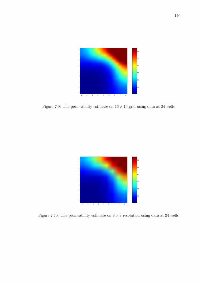
146
0 1 2 3 4 5 6 7 8
0
1
2
3
4
5
6
7
8
10
20
30
40
50
60
Figure 7.9: The permeability estimate on 16× 16 grid using data at 24 wells.
0 1 2 3 4 5 6 7 8
0
1
2
3
4
5
6
7
8
10
20
30
40
50
60
Figure 7.10: The permeability estimate on 8× 8 resolution using data at 24 wells.

147
7.3 Examples
7.3.1 Example I - permeability with bilinear logarithm
In the first example, we apply the one scale Bayesian formulation Eq. (7.9) to
estimate a permeability as shown in Fig. 7.7. A similar problem has been studied in
[51] by modeling the mass transport process as immersible displacement and using
tracer breakthrough time as the data. In the current example, the logarithm of the
permeability field is a linear function of x and y,
logK(x, y) = 0.5(x− 4.0) + 0.5(y − 4.0). (7.15)
The domain is [0.8] × [0, 8]. The parameters in the direct model are µ = 1.0 and
φ = 0.1. The volume injection rate at the injection well is 2.0. At time zero, the con-
centration is zero everywhere except at the injection well ([4,4]). The concentration
at the injection well is kept at 1.0 during the entire time period.
0 1 2 3 4 5 6 7 80
1
2
3
4
5
6
7
8
10
20
30
40
50
60
Figure 7.11: The permeability estimate on 32× 32 resolution using data at 8 wells
without smoothing.
The direct problem is solved on a 32 × 32 grid from time zero until the tracer
is detected at all the production wells. The simulation data are the concentration
values at production wells for all the time. The minimum value of the concentration

148
0 1 2 3 4 5 6 7 80
1
2
3
4
5
6
7
8
10
20
30
40
50
60
Figure 7.12: The permeability estimate on 32× 32 resolution using data at 8 wells
with smoothing.
0 1 2 3 4 5 6 7 8
0
1
2
3
4
5
6
7
8
10
20
30
40
50
60
Figure 7.13: The permeability estimate on 16× 16 resolution using data at 8 wells
with smoothing.
that can be detected is assumed to be 0.0001. Simulation data are generated by
adding random Gauss errors to the direct simulation results. The Gaussian distri-
bution used to generate the errors has a mean of zero and a standard deviation of
5% of the true concentration value. Two cases are considered. In the first situation,
it is assumed that there are 24 production wells evenly distributed at nodes of a
4× 4 grid (a 25-spot problem). In the second case, only 8 production wells as seen
in Fig. 7.1 are considered (a 9-spot problem). The finest permeability estimate is
on a 32× 32 grid in both cases. The scale ratios of unknown permeability to sensor

149
0 1 2 3 4 5 6 7 8
0
1
2
3
4
5
6
7
8
10
20
30
40
50
60
Figure 7.14: The permeability estimate on 8 × 8 resolution using data at 8 wells
with smoothing.
network (M/(√
n− 1)) are 8 and 16 in these two cases, respectively.
In Figs. 7.8, 7.9, and 7.10, the equivalent permeability estimates on 32 × 32,
16 × 16, and 8 × 8 grids are plotted (these three problems are solved separately
using Eq. 7.9). In these estimates, the concentration data at 24 wells (evenly
distributed in the domain) are used. The estimates obtained using concentration
data at only 8 wells (as shown in Fig. 7.1) are plotted in Figs. 7.11 to 7.14. Note
that the plotted results are all the MAP estimates. For the estimates in Figs. 7.12
to 7.14, the results are obtained by applying MRF smoothing to the original MAP
sample. It is seen that the formulation Eq. 7.10 provides rather good estimates of
the regular smooth permeability.
7.3.2 Example II - permeability of a random heterogeneous
medium
In the second example, we apply the two-scale Bayesian posterior distribution de-
veloped in Section 7.2.2 to estimate the random permeability as shown in Fig. 7.2.
In this example, the pressure data at well locations are used instead of the concen-

150
0 2 4 6 80
1
2
3
4
5
6
7
8
0
1
2
3
4
5
6
7
8
Figure 7.15: The coarse scale estimate of the random heterogeneous permeability
(logarithm of the permeability is plotted).
0 2 4 6 80
1
2
3
4
5
6
7
8
0
1
2
3
4
5
6
7
8
2 2.5 3 3.5 44
4.2
4.4
4.6
4.8
5
5.2
5.4
5.6
5.8
6
7.8
7.9
8
8.1
8.2
8.3
4 4.5 5 5.5 62
2.2
2.4
2.6
2.8
3
3.2
3.4
3.6
3.8
4
6.2
6.3
6.4
6.5
6.6
6.7
Figure 7.16: Realization I of the fine scale log permeability distribution. The left
plot is the entire field. The middle plot is the enlarged upper-left darker area
([2, 4]× [4, 6]). The right plot is the enlarged lower-right darker area ([4, 6]× [2, 4]).
tration data. Therefore, in the direct model, only Eqs. (7.1) and (7.2) are solved
with the non-penetrating boundary conditions. Again, the viscosity µ is 1.0 and the
volume injection rate is 2.0. The direct problem is solved on a 128×128 grid, which
is also the resolution of the true permeability. The data are generated by adding
zero mean Gauss random errors to the simulation results (pressure values at well
locations). Again the standard deviation of the distribution used to generate the
random errors is 5 % of the true pressure values. A 25-spot case is considered here

151
0 2 4 6 80
1
2
3
4
5
6
7
8
0
1
2
3
4
5
6
7
8
2 2.5 3 3.5 44
4.2
4.4
4.6
4.8
5
5.2
5.4
5.6
5.8
6
7.8
7.9
8
8.1
8.2
8.3
4 4.5 5 5.5 62
2.2
2.4
2.6
2.8
3
3.2
3.4
3.6
3.8
4
6.1
6.2
6.3
6.4
6.5
6.6
6.7
6.8
Figure 7.17: Realization II of the fine scale log permeability distribution. The
left plot is the entire field. The middle plot is the enlarged upper-left darker area
([2, 4]× [4, 6]). The right plot is the enlarged lower-right darker area ([4, 6]× [2, 4]).
0 2 4 6 80
1
2
3
4
5
6
7
8
0
1
2
3
4
5
6
7
8
2 2.5 3 3.5 44
4.2
4.4
4.6
4.8
5
5.2
5.4
5.6
5.8
6
7.7
7.8
7.9
8
8.1
8.2
8.3
4 4.5 5 5.5 62
2.2
2.4
2.6
2.8
3
3.2
3.4
3.6
3.8
4
6.2
6.3
6.4
6.5
6.6
6.7
Figure 7.18: Realization III of the fine scale log permeability distribution. The
left plot is the entire field. The middle plot is the enlarged upper-left darker area
([2, 4]× [4, 6]). The right plot is the enlarged lower-right darker area ([4, 6]× [2, 4]).

152
0 2 4 6 80
1
2
3
4
5
6
7
8
0
1
2
3
4
5
6
7
8
2 2.5 3 3.5 44
4.2
4.4
4.6
4.8
5
5.2
5.4
5.6
5.8
6
8.03
8.035
8.04
8.045
8.05
8.055
8.06
8.065
8.07
8.075
4 4.5 5 5.5 62
2.2
2.4
2.6
2.8
3
3.2
3.4
3.6
3.8
4
6.435
6.44
6.445
6.45
6.455
6.46
6.465
6.47
6.475
Figure 7.19: Sample mean of the fine scale log permeability distribution. The left
plot is the entire field. The middle plot is the enlarged upper-left darker area
([2, 4]× [4, 6]). The right plot is the enlarged lower-right darker area ([4, 6]× [2, 4]).
(total 25 pressure measurements).
In the first step, the formulation Eq. (7.10) is used to estimate the permeability
on the same length scale as the data collection (a 4× 4 lattice). The result is shown
in Fig. 7.15.
The fine scale permeability is then estimated on a 128 × 128 grid. Three real-
izations (samples from the posterior distribution) of the random permeability are
plotted in Figs. 7.16 to 7.18. The plots are all log permeability values. The sample
mean of 1000 realizations is plotted in Fig. 7.19. Note that the color bars of the
middle and right plots in Fig. 7.19 indicate much smaller intervals than the corre-
sponding color bars in other figures. The mean of these samples is quite close to the
coarse scale estimate. This is a reasonable result since the data do not contain much
information of permeability on length scales smaller than the well distribution. It
only makes sense to estimate the distribution of the fine scale permeability instead
of point estimates.
In addition to the above weakly correlated permeability (ρ = e−r2) example, a
permeability with stronger spatial correlation (ρ = e−|r|) is estimated following the

153
0 1 2 3 4 5 6 7 80
1
2
3
4
5
6
7
8
0
1
2
3
4
5
6
7
8
0 1 2 3 4 5 6 7 80
1
2
3
4
5
6
7
8
7.7
7.8
7.9
8
8.1
8.2
8.3
0 1 2 3 4 5 6 7 80
1
2
3
4
5
6
7
8
6.35
6.4
6.45
6.5
6.55
6.6
6.65
Figure 7.20: True log permeability with correlation coefficient ρ = e−|r|. The left
plot is the entire field. The middle plot is the enlarged upper-left darker area
([2, 4]× [4, 6]). The right plot is the enlarged lower-right darker area ([4, 6]× [2, 4]).
0 1 2 3 4 5 6 7 80
1
2
3
4
5
6
7
8
0
1
2
3
4
5
6
7
8
0 1 2 3 4 5 6 7 80
1
2
3
4
5
6
7
8
8
8.1
8.2
8.3
8.4
8.5
8.6
0 1 2 3 4 5 6 7 80
1
2
3
4
5
6
7
8
6.2
6.3
6.4
6.5
6.6
6.7
Figure 7.21: Realization I of the fine scale log permeability distribution with ρ =
e−|r|. The left plot is the entire field. The middle plot is the enlarged upper-left
darker area ([2, 4] × [4, 6]). The right plot is the enlarged lower-right darker area
([4, 6]× [2, 4]).
exactly same procedure. The distribution for generating random errors is also the
same as the above. The true log permeability and two realizations from the fine
scale posterior distribution are depicted in Figs. 7.20 to 7.22.
7.4 Summary
A multiscale permeability estimation problem is addressed in this chapter using
hierarchical Bayesian analysis and a hierarchical Markov tree (HMT) model. A hy-

154
0 1 2 3 4 5 6 7 80
1
2
3
4
5
6
7
8
0
1
2
3
4
5
6
7
8
0 1 2 3 4 5 6 7 80
1
2
3
4
5
6
7
8
8
8.1
8.2
8.3
8.4
8.5
8.6
8.7
0 1 2 3 4 5 6 7 80
1
2
3
4
5
6
7
8
6.2
6.3
6.4
6.5
6.6
6.7
Figure 7.22: Realization II of the fine scale log permeability distribution with ρ =
e−|r|. The left plot is the entire field. The middle plot is the enlarged upper-left
darker area ([2, 4] × [4, 6]). The right plot is the enlarged lower-right darker area
([4, 6]× [2, 4]).
brid MCMC sampler is designed to explore the high-dimensional two-scale posterior
state space. It is demonstrated though the estimation of a random heterogeneous
permeability using pressure data that the Bayesian formulations are able to provide
distribution estimate of the fine scale permeability using sparse data.

Chapter 8
Conclusions and suggestions for
the future research
An integrated Bayesian and scientific computational framework has been developed
in this thesis for the solution of generic data-driven inverse problems in continuum
transport processes (inverse transport problems). Stochastic modeling of the inverse
transport problems using Bayesian inference method is first introduced via study of
a group of inverse heat conduction problems (IHCPs). An automated regularization
parameter selection method is presented using the hierarchical Bayesian models.
Two-scale Markov Random Field (MRF) and discontinuity adaptive Markov Ran-
dom Field (DAMRF) are used as prior models in addressing inverse problems with
dynamic unknowns and discontinuous unknowns, respectively. Metropolis-Hastings
(MH) algorithms, in particular, the Gibbs sampler and cyclic MH samplers, are in-
troduced for numerical solution of the IHCPs. The fusion of Bayesian computation
and continuum modeling is established via these studies.
For complex nonlinear inverse transport problems, proper orthogonal decompo-
sition (POD) based reduced-order modeling technique is introduced and integrated
155

156
with MH algorithms and parallel computation. The high computational cost asso-
ciated with Bayesian approach to inverse transport problems is addressed. Further,
backward solution to continuum transport process equations and open-loop control
of directional solidification are addressed using sequential Bayesian computational
method. Finally, the multiscale parameter estimation in heterogeneous porous me-
dia flow is address by introducing the hierarchical Markov tree (HMT) model.
It is concluded that the Bayesian approach is able to model and quantify system
and measurement uncertainties in inverse transport problems. Bayesian method
cures the ill-posedness of the inverse problem by posing it as a well-posed problem
in an expanded stochastic space. The usage of spatial statistics models in prior
distribution modeling and the hierarchical Bayesian models allow more flexible reg-
ularization than conventional inverse methods and enable automated selection of the
regularization parameters. It is also concluded that the high computational cost in
Bayesian computational approach can be addressed by using reduced-order modeling
techniques in the exploration of Bayesian posterior distributions. Also, the sequen-
tial Bayesian computational approach is more computationally efficient than the
conventional whole-time domain functional optimization approach in estimation-
prediction of dynamic transport processes. Mutlsicale Bayesian inversion models
provide tools to obtain the distribution and statistics of heterogeneous parameters
with sparse data.
Although this thesis has addressed the fundamental issues of applying Bayesian
computational method to inverse transport problems, several new developments can
broaden the applicability and scope of this approach. Suggestions for the continua-
tion of this study are provided next.

157
8.1 Pattern recognition for reduced-order model-
ing
It has been discussed that POD-based reduced-order modeling is one effective ap-
proach to reduce the computational cost in Bayesian computation. However, the
accuracy of reduced-order modeling depends strongly upon selection of the POD
basis fields. For inverse problem in complex continuum systems, the underlying
physics may vary significantly. Different physics may exist simultaneously such as
the combined heat convection and radiation processes in participating media. Also,
the mathematical models for the same physical process may be different. For in-
stance, the dispersion tensor in an advection-dispersion equation may by isotropic
or anisotropic, homogeneous or inhomogeneous. Furthermore, characteristics of the
same physical process may be completely different for different parameters in the
governing PDEs. For instance, the famous Bernard thermal instability with vari-
ation in thermal Rayleigh number. Therefore, for a complex continuum system
with significant experimental and/or simulation results, it is necessary to develop
an algorithm that can identify the proper POD basis containing the correct physical
modes.
Developing a digital library with associated classification, search and enlarge-
ment abilities is a potential approach to address this issue. Statistical classification
algorithms can be used to train the massive field data for the categorized digital
library. Each branch of the library contains a set of POD basis that corresponds to
a specific physical process with certain parameter range. The proper basis for new
application can be extracted from the library. Considering the high dimensionality
feature of such classification problem, Support Vector Machine (SVM) [106, 107]

158
is deemed as a proper means to conduct the basis model selection task. SVM is
a statistical learning algorithm for pattern classification and regression, which in-
volves training a set of optimal separation hyper-planes from labelled fields belong
to different categories. This development of digital library with associated classifier
will enable the application of Bayesian computation for more generic and complex
inverse continuum problems.
8.2 Enhancing the multiscale Bayesian inversion
techniques
To solve multiscale parameter estimation problems as the permeability estimation
problem discussed in Chapter 7, the key issues are modeling prior distribution of
the heterogeneous parameter at hierarchical length scales, deriving the posterior
distribution that contain parameters and data at all these length scales, allowing
adaptive selection of the basis functions for the discretization, and exploring the
multiscale posterior state space efficiently. A hierarchical Markov tree (HMT) model
has been introduced in this thesis to address the problem under a Bayesian analysis
framework. Some further development may be able to enhance the capability to
deal with more generic multiscale inverse problems.
Firstly, development of adaptive basis function selection method using Bayesian
analysis [108] enables more flexible scheme to model the multiscale parameters. In
addition, it is obvious that both deterministic optimization methods and standard
statistical computation algorithms fail to calculate the statistics of multiscale para-
meter estimates. New algorithms that integrate hybrid MCMC simulation [38] and
multiscale simulation methods are the potential approaches. The major complica-

159
tion of sampling from the multiscale parameter state space is that no MCMC pro-
posal distribution works universally well for all coefficients at different locations and
scales. Hybrid MCMC designation allows using a set of decoupled proposal kernels,
each of which targets at generating samples from a compact region of the multiscale
state space, to compose one mixed kernel analytically. The mixed proposal distrib-
ution guarantees that the entire multiscale posterior state space is explored, while
the direct multiscale simulation methods can be used within the likelihood compu-
tation for each hybrid update step. Hybrid MCMC schemes have to be fused with
multiscale simulation tools to explore the distribution with the abilities of i) gener-
ating samples of parameter projections at all length scales efficiently; ii) spending
more sampling steps in the regions and length scales with high heterogeneity; iii)
projecting distribution on one scale upward and downward to other scales; and iv)
updating the distribution with consecutively achieved data.
8.3 Wavelet function representation
In all of the examples in this thesis, finite element basis functions are used for
discretization of the inverse solution. This is not the optimal strategy in applications
where the inverse solution is multiscale in nature. The wavelet domain method
provides better sets of basis for such inverse problems [109].
Wavelet basis functions can represent function spaces at all length scales. The
unresolved residue can be quantified using its projection at the minimum resolved
length scale. It is a consistent choice for parametrization of multiscale inverse so-
lutions. By linking with mutual information theory and Maximum Entropy theory,
the proper minimum resolved length scale and statistics of multiscale parameter

160
can be estimated. Therefore, it is expected by introducing wavelet basis function to
Bayesian inverse computation, broader applications can be achieved.

Bibliography
[1] J. V. Beck, B. Blackwell and C. R. St-Clair Jr., Inverse Heat Conduction:
Ill-posed Problems, Wiley-Interscience, New York, 1985.
[2] R. Siegel and J.R. Howell., Thermal Radiation Heat Transfer, 3rd Edt., Hemi-
sphere publishing corporation, 1992.
[3] O. M. Alifanov, Inverse Heat Transfer Problems, Springer-Verlag, Berlin, 1994.
[4] M. N. Ozisik and R. B. Orlande., Inverse Heat Transfer: Fundamentals and
Applications, Taylor & Francis pbulication, 2000.
[5] K. A. Woodbury. (Edt.), Inverse Engineering Handbook 1st edition, CRC
Press, 2002
[6] N. Zabaras, Inverse problems in heat transfer, Chapter 17, Handbook of
Numerical Heat Transfer, 2nd Edt., John Wiley and Sons, 2004. (W.J.
Minkowycz, E.M. Sparrow, J. Y. Murthy, Edts.)
[7] N. Zabaras and S. Kang, On the Solution of An Ill-posed Inverse Design Solidi-
fication Problem Using Minimization Techniques in Finite and Infinite Dimen-
sional Spaces, International Journal for Numerical Methods in Engineering,
36:3973-3990, 1993.
161

162
[8] R. Sampath and N. Zabaras, Inverse thermal design and control of solidifica-
tion processes in the presence of a strong external magnetic field, International
Journal for Numerical Methods in Engineering, 50:2489-2520, 2001.
[9] R. Sampath and N. Zabaras, A functional optimization approach to an inverse
magneto-convection problem, Compt. Meth. Appl. Mech. Eng., 190:2063–2097,
2001.
[10] A.N. Tikhonov, Solution of incorrectly formulated problems and the regular-
ization method, Soviet Math. Dokl., 4(4):1035-1038, 1963.
[11] A.N. Tikhonov, Regularization of incorrectly posed problems, Soviet Math.
Dokl., 4(6):1624-1627, 1963.
[12] A. N. Tikhonov, Solution of ill-posed problems, Halsted Press, Washington,
1977.
[13] N. Zabaras, and J.C. Liu, An analysis of two-dimensional linear inverse heat-
transfer problems using an integral method, Num. Heat Transfer, 13(4):527-
533, 1988.
[14] F. Hettlichy and W. Rundell, Iterative methods for the reconstruction of an
inverse potential problem, Inverse Problems, 12:251-266, 1996.
[15] D.A. Murio, The Mollification Method and the Numerical Solution of Ill-posed
Problem, Wiley, New York, 1993.
[16] P. M. Norris, Application of experimental design methods to assess the efect
of uncertain boundary conditions in inverse heat transfer problems, Int. J.
Heat Mass Transfer, 41:313-322, 1998.

163
[17] B. F. Blackwell and K. J. Dowding., Sensitivity and uncertainty analysis for
thermal problems, Preceedings of the 4th International Conference on Inverse
Problems in Engineering Rio de Janeiro, Brazil, 2002
[18] T. D. Fadale, A. V. Nenarokomov and A. F. Emery, Uncertainties in parameter
estimation: the inverse problem, Int. J. Heat Mass Transfer, 38(3):511-518,
1995.
[19] A. F. Emery, A. V. Nenarokomov and T. D. Fadale, Uncertainties in para-
meter estimation: the optimal experiment design, Int. J. Heat Mass Transfer,
43:3331-3339, 2000.
[20] V. A. Badri Narayanan and N. Zabaras, Stochastic inverse heat conduction
using a spectral approach, Int. J. Numer. Meth. Eng., 60(9):1569-1593, 2004.
[21] A. F. Emery, Stochastic regularization for thermal problems with uncertain
parameters, Inverse Problems in Engineering, 9:109-125, 2001.
[22] C. Ferrero and K. Gallagher, Stochastic thermal history modeling, 1. con-
straining heat flow histories and their uncertainty, Marine and Petroleum Ge-
ology, 19:633-648, 2002.
[23] N. Leoni and C.H. Amon, Bayesian surrogates for integrating numerical, ana-
lytical and experimental data: application to inverse heat transfer in wearable
computers, IEEE Transactions Comps. Pack. Manuf. Technology, 23:23-33,
2000.
[24] C. P. Robert, The Bayesian Choice, From Decision-Theoretic Foundations to
Computational Implementation, 2nd Edt., Springer, 2001.

164
[25] J. Besag, P. Green, D. Higdon and K. Mengersen, Bayesian computation and
stochastic systems, Statistical Science, 10(1):3-41, 1995.
[26] P. Congdon, Bayesian Statistical Modeling, Wiley, New York, 2001.
[27] J. P. Kaipio and E. Somersalo, Computational and Statistical Methods for
Inverse Problems, Springer-Verlag, New York, 2005.
[28] C. Vogel, An applied mathematician’s perpective on regularization methods,
lecture in opening workshop for inverse problem methodology in complex sto-
chastic models, Session of parameter estimation and inverse problems, sta-
tistics perspective, Statistical and Applied Mathematical Sciences Institute,
Duke University, 2002.
[29] J. Wang and N. Zabaras, A Bayesian inference approach to the stochastic
inverse heat conduction problem, International Journal of Heat and Mass
Transfer, 47:3927-3941, 2004.
[30] J. Wang and N. Zabaras, A Markov Random Field model of contamination
source identification in porous media flow, International Journal of Heat and
Mass Transfer, accepted for publication.
[31] J. Wang and N. Zabaras, Hierarchical Bayesian models for inverse problems
in heat conduction, Inverse Problems, 21:183-206, 2005.
[32] J. Wang and N. Zabaras, Using Bayesian statistics in the estimation of heat
source in radiation, International Journal of Heat and Mass Transfer, 48:15-
29, 2005.
[33] J. Besag and C. Kooperberg, On the conditional and intrinsic autoregressions,
Biometrika, 82:733-746, 1995.

165
[34] J. Møller (Edt.), Spatial Statistics and Computational Methods, Springer-
Verlag, New York, 2003.
[35] J. Mateu and F. Montes (Edts.), Spatial Statistics Through Applications, In-
ternational Series on Advances in Ecological Sciences, WITPress, Boston,
2002.
[36] J. Besag and R. A. Kempton, Statistical analysis of field experiments, Bio-
metrics, 78:301-304, 1986.
[37] J. Besag and P. J. Green, Spatial statistics and Bayesian computation, Journal
of the Royal Statistical Society, Series B, Methodological, 55:25-37, 1993.
[38] C. Andrieu, N. Freitas, A. Doucet and M. I. Gordan, An introduction to
MCMC for machine learning, Machine Learning, 50:5-43, 2003.
[39] J. S. Liu, Monte Carlo Strategies in Scientific Computing, Springer-Verlag,
Berlin, 2001.
[40] P. Bremaud, Markov Chains, Gibbs Fields, Monte Carlo Simulation, and
Queues, Springer-Verlag, New York, 1999.
[41] P. J. Van Laarhoven and E. H. L. Arts, Simulated Annealing: Theory and
Applications, Reidel Publishers, Amsterdam, 1987.
[42] L. Tierney, Markov chains for exploring posterior distributions, The Annals
of Statistics, 22(4):1701-1762, 1994.
[43] W. R. Gilks, S. Richardson and D. J. Spiegelhalter(Edt.), Markov Chain
Monte Carlo in Practice, Chapman & Hall Ltd, New York, 1996.

166
[44] I. Beichl and F. Sullivan, The Metropolis algorithm, Computing in Science
and Engineering, 2(l):65-69, 2000.
[45] J. L. Beck and S. K. Au, Bayesian updating of structural models and reliabil-
ity using Markov Chain Monte Carlo Simulation, J Engineering Mechanics,
128:380-391, 2002.
[46] J. P. Kaipio, V. Kolehmainen, E. Somersalo and M. Vauhkonen, Statistical
inversion and Monte Carlo sampling methods in electrical impedance tomog-
raphy, Inverse Problems, 16: 1487-1522, 2000.
[47] T. J. Sabin, C. A. L. Bailer-Jones and P.J. Withers, Accelerated learning using
Gaussian process models to predict static recrystallization in an Al-Mg alloy,
Modeling Simul. Mater. Sci. Eng., 8:687-706, 2000.
[48] A. M. Michalak and P. K. Kitanidis, A method for enforcing parameter non-
negativity in Bayesian inverse problems with an applicaiton to contaminant
source identification, Water Resour. Res., 39:1033-1046, 2003
[49] I. G. Osio, Multistage Bayesian Surrogates and Optimal Sampling for En-
gineering Design and Process Improvement, Ph.D. Thesis, Carnegie Mellon
University, Pittsburgh, PA, 1996
[50] D. Higdon, H. K. Lee and Z. Bi, A Bayesian approach to characterizing un-
certainty in inverse problems using coarse and fine-scale information, IEEE
Transactions on Signal Processing, 50(2):389-399, 2002.
[51] H. K. Lee, D. M. Higdon, Z. Bi, M. A.R. Ferreira and M. West, Markov
random field models for high-dimensional parameters in simulations of fluid
flow in porous media, Technometrics, 44 (3):230-241, 2002.

167
[52] R. Chellappa and A. Jain (Edts), Markov Random Fields Theory and Appli-
cation, Academic Press Inc., 1991.
[53] S. Geman and D. Geman, Stochastic relaxation, Gibbs distributions and the
Bayesian restoration of images, Transactions on Pattern Analysis and Machine
Intelligence, 6:721-741, 1984.
[54] S. P. Brooks and G. O. Roberts, Convergence assesment techniques for Markov
Chain Monte Carlo, Statistics and Computing, 8:319-335, 1998.
[55] J. V. Beck and K. J. Arnold, Parameter Estimation in Engineering and Sci-
ence, New York: Wiley, 1977.
[56] J. R. Cannon and P. DuChateau, Inverse problems for an unknown source in
heat equation. J Mathematical Analysis and Applications, 75:465-485, 1980
[57] V. Isakov, Inverse Source Problems, American Mathematical Society, 1990
[58] A. Nanda and P. Das, Determination fo the source term in the heat conduction
equation, Inverse Problems, 12:325-339, 1996.
[59] D. J. Kang and K. S. Roh, A discontinuity adaptive Markov model for color
image smoothing, Image and Vision Computing, 19:369-379, 2001
[60] S. Z. Li, Discontinuous MRF prior and robust statistics: a comparative study,
Image and Vision Computing, 13:227-233, 1995
[61] Z. Yi and D. A. Murio, Source terms identification for the diffusion equa-
tion, 4th International Conference on Inverse Problems in Engineering Rio de
Janeiro, Brazil, 2002.

168
[62] P. Holmes, J. L. Lumley and G. Berkooz, Turbulence, Coherent Structures,
Dynamical Systems and Symmetry, Cambridge University Press, 1998.
[63] M. F. Modest, Radiative Heat Transfer, McGraw-Hill, Inc., 1993.
[64] C. H. Ho, M. N. Ozisik, An inverse radiation problem, International Journal
of Heat and Mass Transfer, 32:335-341, 1989.
[65] N. J. McCormick, Inverse radiative transfer problems : a review, Nuclear
Science and Engineering, 112:185-198, 1992.
[66] H. E., Ofodike, A. Ezekoye and J. R. Howell, Comparison of three regularized
solution techniques in a three-dimensional inverse radiation problem, Journal
of Quantitative Spectroscopy and Radiative Transfer, 73:307-316, 2002.
[67] L. H. Liu and H. P. Tan, Inverse radiation problem in three-dimensional com-
plicated geometric systems with opaque boundaries, Journal of Quantitative
Spectroscopy and Radiative Transfer, 68:559-573, 2001.
[68] C. E. Siewert, An inverse source problem in radiative transfer, Journal of
Quantitative Spectroscopy and Radiative Transfer, 50:603-609, 1993.
[69] T. Viik and N. J. McCormick, Numerical test of an inverse polarized radia-
tive transfer algorithm, Journal of Quantitative Spectroscopy and Radiative
Transfer, 78:235-241, 2003.
[70] M. Prud’homme and S. Jasmin, Determination of a heat source in porous
medium with convective mass diffusion by an inverse method, International
Journal of Heat and Mass Transfer, 46:2065-2075, 2003.

169
[71] H. M. Park and T. Y. Yoon, Solution of the inverse radiaiton problem using a
conjugate gradient method, International Journal of Heat and Mass Transfer,
43:1767-1776, 2000.
[72] S. M. H. Sarvari, J. R. Howell, and S. H. Mansouri, Inverse boundary design
conduction-radiation problem in irregular two-dimensional domains, Numeri-
cal Heat Transfer Part B - Fundamentals, 44(3):209-224, 2003.
[73] S. Subramaniam and M. P. Menguc, Solution of the inverse radiation problem
for inhomogeneous and anisotropically scattering media using a Monte Carlo
technique, International Journal of Heat and Mass Transfer, 34:253-266, 1991.
[74] A. N. Brooks and T. J. R. Hughes, Streamline-upwind/Petrov-Galerkin formu-
lation for convection dominated flows with particular emphasis on the incom-
pressible Navier-Stokes equation, Comput. Methods Appl. Mech. Eng., 32:199-
259, 1982.
[75] H. M. Park and M. C. Sung, Sequential solution of a three-dimensional inverse
radiation problem, Compt. Meth. Appl. Mech. Eng., 192:3689-3704, 2003.
[76] S. S. Ravindran, A reduced-order approach for optimal control of fluids using
proper orthogonal decomposition, International Journal for Numerical Meth-
ods in Fluids, 34:425-448, 2000.
[77] H. V. Ly and H. T. Tran, Modeling and control of physical processes us-
ing proper orthogomal decomposition, Mathematical and Computer Modeling,
33:223-236, 2001.
[78] J. Atmadja and A. C. Bagtzoglou, Pollution source identification in heteroge-
neous porous media, Water Resources Research, 37: 2113-2125, 2001.

170
[79] A. M. Michalak and P. K. Kitanidis, Estimation of historical groundwater con-
taminant distribution using the adjoint state method applied to geostatistical
inverse modeling, Water Resources Research, 40, W08302, 2004.
[80] M. F. Snodgrass and P. K. Kitanidis, A geostatistical approach to contaminant
source identification, Water Resources Research, 33:537-546, 1997.
[81] A. M. Michalak and P. K. Kitanidis, Application of geostatistical inverse mod-
eling to contaminant source identification at Dover AFB, Delaware, Journal
of Hydraulic Research, 42:9-18, 2004.
[82] C. Crainiceanu, D. Ruppert, J.R. Stedinger and C.T. Behr, Improving MCMC
mixing for a GLMM describing pathogen concentrations in water supplies,
Case Studies in Bayesian Statistics, VI, Gatsonis, C., et al (editors), Lecture
Notes in Statistics, 167:207-222, 2002.
[83] C. Crainiceanu, J. Stedinger, D. Ruppert and C. Behr, Modeling the U. S. na-
tional distribution of waterborne pathogen concentrations with application to
cryptosporidium parvum, Water Resources Research, 39(9):1235-1249, 2003.
[84] A. F.D. Loula, F. A. Rochinha and M. A. Murad, Higher-order gradient post-
processing for second-order elliptic problems, Computer Methods in Applied
Mechanics and Engineeeing, 128:361-381, 1995.
[85] H. Wang, D. Liang, R. E. Ewing, S. L. Lyons and G. Qin, An ELLAM-
MFEM solution technique for compressible fluid flows in porous media with
point sources and sinks, Journal of Computational Physics, 159:344-376, 2000.
[86] A. L.G.A. Coutinho and J. L.D. Alves, Parallel finite element simulation of
miscible displacement in porous media, SPE Journal, 1:487-500, 1996.

171
[87] S. Balay, K. Buschelman, V. Eijkhout, W.D. Gropp, D. Kaushik, M.G. Kne-
pley, L.C. McInnes, B.F. Smith and H. Zhang, PETSc Users Manual, ANL-
95/11 - Revision 2.1.5, Argonne National Laboratory, 2004.
[88] A.L.G.A. Coutinho, C.M. Dias, J.L.D. Alves, L. Laudau, A.F.D. Loula,
S.M.C. Malta, R.G.S. Castro and E.L.M. Garcia, Stabilized methods and
post-processing techniques for miscible displacements, Computer Methods in
Applied Mechanics and Engineering, 193:1421-1436, 2004.
[89] R.G. Sanabria Castro, S.M.C. Malta, A.F.D. Loula and L. Landau, Numerical
analysis of space-time finite element formulations for miscible displacements,
Computational Geosciences, 5:301-330, 2001.
[90] O. Patzold, I. Grants, U. Wunderwald, K. Jenker, A. Croll and G. Gerbeth,
Vertical gradient freeze growth of GaAs with a rotating magnetic field, J.
Crys. Growth, 245:237-246, 2002.
[91] J.K. Roplekar and J.A. Dantzig, A study of solidification with Rotating Mag-
netic field, UMinn report 2000.
[92] V. Galindo, G. Gerbeth, W. Von Ammon, E. Tomzig and J. Virbulis, Crystal
growth melt flow control by means of magnetic fields, Energy Conv. Manage.,
in press.
[93] H.P. Utech and M.C. Flemings, Elimination of Solute Banding in Indium
Antimonide Crystals by Growth in a Magnetic Field, J. App. Phys., 7:2021-
2024, 1966.

172
[94] H.A. Chedzey and D.T.J. Hurle, Avoidance of Growth-Striae in Semiconductor
and Metal Crystals Grown by Zone-Melting Techniques, Nature, 210:933-934,
1966.
[95] G.M. Oreper and J. Szekely, The effect of a magnetic field on transport phe-
nomena in a Bridgeman-Stockbarger crystal growth, J. Crys. Growth, 67:405-
435, 1984
[96] S. Motakef, Magnetic field eliminitation of convective interference with segre-
gation during vertical Bridgeman growth of doped semi-conductors, J. Crys.
Growth, 64:550-563, 1990
[97] H. Ben Hadid and B. Roux, Numerical study of convection in the horizontal
Bridgeman configuration under the action of a constant magnetic field. 1. Two
dimensional flow, J. Fluid Mech., 333:23-56, 1997
[98] H. Ben Hadid and B. Roux, Numerical study of convection in the horizontal
Bridgeman configuration under the action of a constant magnetic field. 2.
Three dimensional flow, J. Fluid Mech., 333:57-83, 1997.
[99] J. W. Evans, C. D. Seybert, F. Leslie and W. K. Jones, Supression/reversal
of natural convection by exploiting the temperature/composition dependance
of magnetic susceptibility, J. App. Phys., 88(7):4347-4351, 2000.
[100] J. Huang, D.D. Gray and B.F. Edwards, Thermoconvective instability of para-
magnetic fluids in a nonuniform magnetic field, Phys. Rev E, 57:5564-5571,
1998.

173
[101] B. Ganapathysubramanian and N. Zabaras, Using magnetic field gradients to
control the directional solidification of alloys and the growth of single crystals,
J. Crys. Growth, submitted for publication.
[102] B. Ganapathysubramanian, N. Zabaras, Control of solidification of non-
conducting materials using tailored magnetic fields, J. Crys. Growth, sub-
mitted for publication.
[103] C. Collet and F., Murtagh, Multiband segmentation based on a hierarchical
Markov model, Pattern Recognition, 37:2337-2347, 2004.
[104] M. S. Crouse, R. D. Nowak and R. G. Baraniuk, Wavelet-based statisticsl
signal processing using Hidden Markov Models, IEEE Transactions on Signal
Processing, 46:886-902, 1997.
[105] A.A. Grimstad, T. Mannseth T., G. Navdal and H. Urkedal, Adaptive multi-
scale permeability estimation, Computational Geosciences, 7(1):1-25, 2003.
[106] S. Dumais, Using SVMs for text categorization, IEEE Intell. Systems, 13:21-
23, 1998.
[107] T. Joachims, Learning to Classify Text using Support Vector Machines,
Kluwer, 2002.
[108] C.M. Crainiceanu, D. Ruppert and R.J. Carroll, Spatially adaptive P-spline
with heteroscedastic errors, submitted to Journal of Computational and
Graphical Statistics.
[109] J. Liu and P. Moulin, Information Theoretic analysis of interscale and in-
trascale dependencies between image wavelet coefficients, IEEE transactions
on image processing, 10(11):1647-1658, 2001.