Forecasting fire dynamics using inverse Computational Fluid Dynamics

modelling and Tangent Linearisation

W. Jahna, G. Reina,, J.L. Toreroa

aSchool of Engineering, The University of Edinburgh,King’s Buildings, Edinburgh, EH9 3JL, UK.

Abstract

A technology able to forecast fire dynamics in buildings would lead to a paradigm shift in the response to emergencies,

providing the Fire Services with essential information about the ongoing blaze with some lead time (i.e. seconds or

minutes ahead of the event). But the state-of-the-art of Computational Fluid Dynamics in fire dynamics is not fast nor

accurate enough to provide valid predictions on time. This paper presents a methodology to forecast fire dynamics

using Computational Fluid Dynamics based on assimilation of sensor observations. The forecast is posed as an inverse

problem to solve for the invariants governing the dynamics, and a tangent linear approach is used in the optimisation.

The forward fire model is linearized in order to obtain a quadratic cost function that is easily minimised. A series of

real-scale compartment fire cases are investigated using the Computational Fluid Dynamics code FDSv5 together with

synthetic data. Up to three different invariant are considered (spread rate, burning rate and soot yield) in scenarios

with one or two fires and different origins. The effect of density, location and type of sensors is studied. It is shown

that the use of coarse grids in the forward model significantly accelerates the assimilation up to 100 times without

loss of forecast accuracy due to the aid of sensor data. This provides close to positive lead times using Computational

Fluid Dynamics. These results are a fundamental step towards the development of forecast technologies able to lead

the fire emergency response.

Keywords: Fire modelling, forecast, data driven simulation, gradient based optimization, tangent linear

1. Introduction

Forecasting compartment fire dynamics is a subject

of research interest in fire safety science. After preven-

tion, the first line of response to a fire event is part of the

design process of a building in the form of detection,

compartmentation, ventilation, egress paths, suppres-

sion and structural resistance1. But accidental fires that

overcome these measures occur with some frequency,

and it is necessary to prepare for that case and protect

life and property against the detrimental effects of heat

and smoke produced. When a fire escalates, interven-

tion of the Fire Service takes place and management of

the scene is delegated to them. The fire fighting strat-

egy to follow is currently based mostly on the experi-

ence and the intuition of the commanding officers on

duty. This offers space for improvement. In particular,

it would be a great advantage if decisions could be based

as well on short- and medium-term forecasts of the fire

development. Not only would this allow for more effi-

cient strategies, saving lives and reducing damage and

cost, it would also improve the safety of fire fighters.

The tragic events on 9/11 after the attacks of the World

Trace Center are an example where prior knowledge

of fire development and structural response would have

been essential for the Fire Service.

Modern buildings already provide some limited in-

formation about an ongoing fire emergency, including

security cameras and security panels which could indi-

cate in a rudimentary manner the origin and magnitude

of the event. The currently low density and crude na-

ture of buildings sensor data, however, makes reliance

on experience and intuition for fire fighting unavoid-

able2. In the near future, the role of intelligent building

systems is expected to be central for the modern built

environment. These systems are designed to monitor

with sensors and control the performance of mechani-

cal and electrical elements, and can easily be extended

to include fire safety3.

Cowlard et al. 2 have suggested the use of fire model

predictions to assist emergency response. They postu-

late that the forecasting of fire dynamics in compart-

ments would imply a paradigm shift in the response

to emergencies, providing the Fire Service with essen-

tial information about the emergency development with

some lead time (ahead of the event).

If computational models are ever to forecast fire in

support of emergency response, the computational time

has to be shorter than the event itself. From a fire fight-

ing point of view, forecasting of fire only makes sense

if it arrives with a positive lead time, i.e. data is as-

similated and a satisfactory prediction is produced faster

than the fire is evolving. But the state-of-the-art of com-

putational fluid dynamics (CFD) for fire demands heavy

computational resources and large computing times that

are far greater than the times associated with fire dynam-

ics (hours to model seconds). Moreover, the accuracy

of the computer predictions of fire is poor due to the

complex nature of the governing physical and chemical

processes4,5.

2. Inverse Modelling

Even if all the governing mechanisms could be solved

from first principles, the chaotic nature of fire imposes a

maximum possible lead time to the forecast, as has been

shown for other dynamic systems like weather6. This

suggests that fire modelling alone cannot be used for

emergency response without feedback information from

the evolving fire. Moreover, models complemented

with sensor data have the potential to achieve the re-

quired speed, precision and robustness7. It has been

proposed to use sensor data as a substitute for modelling

fine details, thus enabling simpler approaches to provide

fast and useful outputs8. Continuous correction of the

model output by means of sensor data allows for steer-

ing of the models to account for uncertainty in the input

variables and for changes in the environment (e.g. win-

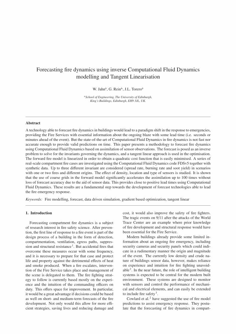
dow breakage or flashover). This concept is illustrated

in fig. 1, where sensor data is continuously assimilated

in time to simulate the fire evolution and steer the com-

putations.

The use of sensor data to estimate model parameters

is generally known as inverse modelling. Parameter es-

timation and inverse modelling are an important area

within the engineering and scientific community.

In numerical weather predictions (NWP) inverse

modelling and data assimilation take up an important

part of the computational resources10. In order to ini-

tialize the numerical models that are used to forecast

the state of the atmosphere, weather observations from

several places over the planet are collected and then as-

similated into the model. Observations are assimilated

����������� ���

���������

�� � �

������

�� � �

������

�� � �

�������� � �

������

�� � �

������

���������

���������

�� ���������� ���

����������������

���������������

���������

Figure 1: Conceptual representation of the data assimi-

lation process and the sensor steering of model predic-

tions even when fundamental changes take place in an

evolving emergency scenario9.

by initializing a new forecast based on a previous fore-

cast (several hours back), and correcting it according to

the difference between the previous forecast and the ob-

servations11,12. Most modern NWP systems assimilate

observations during a certain period of time (assimila-

tion window) before starting the forecast13. The assimi-

lation algorithm typically involves a linearization of the

NWP system around the previous forecast and the sub-

sequent solution of a quadratic minimization problem10.

The basic principles of this methodology, called the tan-

gent linear model (TLM), are applied in this work, ad-

justed to the specific features of fire dynamics.

In fire science, several inverse modelling studies have

been undertaken. Richards et al. 14 use a database of pre-

run zone-type models to estimate fire location and fire

growth. They use the same zone model to generate the

data for comparison, and analyze the influence of mea-

surements and modelling errors. Leblanc and Trouve

use a zone model to predict the heat release rate (HRR)

time-history based on observations generated using the

same model15. While they are able to closely reproduce

the HRR history, their work does not address the fore-

casting of future events.

Cowlard et al. 7 use a semiempirical correlation and

multiple flame front observations to predict upward

flame spread over a small-scale fuel slab. They were

able to estimate correctly the parameter values and

make predictions in super-real-time (i.e. with a posi-

tive lead time). Koo et al. 16 used measurements from

a large-scale fire test to progressively steer zone model

simulations towards effective parameter values using a

Monte Carlo approach and a set of random generated

scenarios. The model is able to reproduce satisfactorily

past observations of temperature.

A conceptual framework for forecasting of fire

growth has been proposed by Jahn9. The forecast is

posed as an inverse problem to solve for the invariants

2

governing the dynamics, and a minimisation technique

is used. It has been applied to compartment fire using

a zone model8, which rapidly estimated the correct in-

variants, but the forecasts were limited by the general-

izations of the simple model. The present paper builds

upon previous work and applies inverse modelling us-

ing CFD. The forward fire model (FDSv5) is linearized

in order to obtain a quadratic cost function that is easily

minimized. In order to demonstrate the performance of

the approach, a series of realistic compartment fire cases

are investigated. Further application of CFD forecasting

to a real fire experiment is shown in17. These results are

a fundamental step towards the development of forecast

technology able to lead the fire emergency response.

In this document a conceptual framework and a math-

ematical methodology is proposed to allow for forecast-

ing of fire growth. The highly complicated interaction

between gas and solid phase are replaced by a simpli-

fied fire growth model that is input into the gas phase

model as a boundary condition. This growth model is

based on a set of parameters that do not depend on the

feedback from the fire and are thus constant (at least for

a certain amount of time). Observations from the evolv-

ing fire provide the information for the estimation of the

parameters for the growth model.

3. Fire Dynamics

Natural fires in real-size compartments involve mech-

anisms that develop in length-scales ranging from mi-

crometres (flame thickness) to metres (compartment

size), and time-scales from milliseconds (chemistry) to

minutes (burnout)1. Fire dynamics are governed by

complex, strongly coupled physical and chemical pro-

cesses constituting a feedback cycle. Pyrolysis vapours

are produced in the thermal decomposition of the solid

fuel as a result of heat transferred from the flame. The

pyrolyzate is then transported into the flame where it

mixes with fresh oxygen and burns. This results in heat

that is transferred back to the fuel to produce more py-

rolyzate1.

Two fundamentally distinct regimes can be observed

in a compartment fire. Each has to be treated differ-

ently. First a fuel controlled regime, and then a ventila-

tion controlled regime (pre- and post-flashover respec-

tively). The difference between both stages is illustrated

in fig. 2. During the initial fuel controlled regime, suf-

ficient air supply is available to feed the fire, and its

spread rate is not governed by the ventilation, but by

fuel load and arrangement. Boundary conditions are

important only in the proximity of the flames, and the

size and detailed geometry of the compartment does not

greatly affect the course of the fire. For good forecast,

modelling emphasis must be on the growth rate and the

flame geometry.

(a) Fuel controlled fire

(b) Ventilation controlled fire

Figure 2: Different stages of the fire. a) shows a fuel

controlled, localized fire, while b) shows a ventilation

controlled fire.

As the fire grows beyond certain size, the compart-

ment boundaries and the ventilation conditions start

playing an essential role and the fire becomes controlled

by the supply of air. At some point flashover will occur,

after which external flaming takes place at the openings

(doors, windows), as shown in fig. 2b. In a ventilation

controlled regime, good forecasts require emphasis on

the ventilation conditions and fire growth becomes sec-

ondary.

This work is focused on the fuel controlled regime

during which the flame spread rate is the primary in-

variant to estimate growth rate.

4. Fire Modelling

In fire CFD modelling, the gas-phase dynamics are

solved with a specific form of Navier-Stokes for buoy-

ancy driven, low Mach number flows18,19. This is typi-

cally coupled with a mixture fraction model for combus-

tion. Smoke movement and temperature distributions

3

can only be reproduced reasonably well if the curve of

HRR is known4,20,21.

Fire modelling typically handles compartment length

scales of around 10 m. Although depending on the size

of the fire, with a large eddy simulation (LES) approach

a grid resolution between 1 cm and 10 cm in the gas

phase is generally required to obtain sufficient spatial

resolution19. Thus, the computational cost of modelling

fire is considerable.

The fire growth is given by the HRR which is gov-

erned by the spread of the flames over the solid fuel.

While flame spread can be reproduced with numeri-

cal models to considerable accuracy for small flames

(∼ 10 cm) by solving for the pyrolysis of the solid

fuel22,23, it is much less accurate and computationally

more expensive to do so in compartment, as the domain

typically consists of dozens of metres, but grid cells of

the order of millimetres would be required for the mod-

elling of the flaming and pyrolizing regions. A recent

study has shown that flame spread modelling is not sat-

isfactorily at a scale that can be used in real scale fire

scenarios5, even using a relatively fine grid (2.5 cm).

Flame spread and fire growth modelling are subject to

ongoing research and have not been implemented satis-

factorily yet4.

The limitations of state-of-the-art fire growth mod-

elling are thus an important constraint to the forecast

capabilities of fire simulations. It is proposed in this ar-

ticle to decouple the gas phase from the solid phase by

imposing the fire growth as a time dependant boundary

condition to the gas phase modelling. The interaction

between gas and solid phase is replaced by a simplified

fire growth model, which is explained in the following

section.

5. Fire Growth

It can be assumed that the radius of the burning area

(fire size) of an isotropic fuel grows at a constant rate.

This is a reasonable assumption for early fire devel-

opment when flames do not penetrate into the smoke

layer and radiative heat from the walls do not accel-

erate spread24. The fire source becomes thus a time

dependent boundary condition to the gas phase simula-

tion. Assuming a horizontal fire that starts at one point

and spreads outwards radially with a spread rate r (m/s),

and assuming a constant fuel burning rate per unit area

ω (kg/s ·m2), the rate of heat release becomes propor-

tional to the area of the fire, which grows as a function

of the spread rate and of time,

Q = Δhcm = ΔhcωA(r, t), (1)

where Δhc is the effective heat of combustion (in kJ/kg).

As long as the fire does not reach the boundaries of the

fuel surface the fire area is circular (A(r, t) = π(r(t −t0))2). Or it could have form of a fraction of a circle, if

the ignition point is e.g. at the wall. In both cases the

resulting HRR follows a quadratic growth.

This is a first approximation to simulate fire growth.

It avoids direct coupling of gas and solid phase. A sim-

ilar approach is widely used in fire safety engineering,

although the governing parameters are summarized into

a constant α that is tabulated for different materials and

leads to what is known as an “αt2” fire.

For real fuel packages (such as sofas, beds or other

furniture), which consist of several finite surfaces each

with a potentially different spread rate, this approxima-

tion has shown to still hold to a reasonable degree25, and

the constant α corresponds in that case to an equivalent

growth rate.

In fire field models the spread rate r can be pre-

scribed, so that adjacent cells are ignited producing a

fire area that grows at rate r. This will then result in a

fire that grows according to eq. (1).

6. Inverse Modelling

6.1. Framework

In order to be able to predict the state of a physi-

cal system, it is necessary to identify a set of parame-

ters that characterize the system, and that do not change

over time (or change only due to external intervention).

These parameters are the invariants of the system, and

a good forecast relies on good a estimation of these. A

typical forecast cycle thus includes a data collection pe-

riod, an assimilation period where the invariants are es-

timated, and finally a forecast based on those estimated

parameters.

When modelling a physical process from first prin-

ciples, the initial and boundary conditions constitute

the only invariants, and changes of these conditions are

only due to external intervention (for example a peri-

odic boundary condition). In that case the invariants

are well established. However, physical systems cannot

generally be modelled from first principles, and approx-

imations have to be introduced, resulting in additional

invariants that have to be input into the model. These

invariants are normally obtained experimentally.

In the present case the pyrolysis process is replaced

by a fire growth model which results in a boundary con-

dition that changes over time according to eq. (1). The

invariants of interest are the spread rates of the burning

items, the fuel burning rates and other parameters such

4

as soot yield, radiative fraction (related to other approx-

imations in the model).

The problem can thus be represented on the basis of

these invariants summarized in the vector θ:

θ =[r1, r2, . . . , ω1, ω2, . . . , χR,1, χR,2 . . .

].

Once a fire has been detected and observations are

collected during the assimilation window, the relevant

invariants in θ are estimated and a forecast of the fire

development is made without solving the complex inter-

actions between gas and solid phases. The assimilation

window is the period of time where observations are re-

ceived and considered for the optimisation step. As time

goes by, new observations come in, providing more in-

formation on the history of the fire development. In the

present work the term observation refers to sensor data

such as temperature or smoke obscuration.

The methodology is general and any forward model

that represents the system to be simulated can be used.

For scenarios described in this work and the level of

detail required in the approach presented in this article,

a CFD type fire model is used.

6.2. Cost Function

Data are assimilated into the model by minimizing

a cost function that measures the distance between the

model output and the observations. The governing

parameters are then adjusted until convergence is ob-

tained. Several different physical observations can be

used, but temperature and smoke obscuration are used

here because they are the easiest to measure satisfacto-

rily with current technology. The cost function is then

defined as the sum of the distances between model out-

put for a given set of parameters and the measurements:

J(θ) =N∑

i

[yi − yi(θ)

]T Wi[yi − yi(θ)

], (2)

where yi is the set of physical variables that is measured,

and yi(θ) is the output of the forward integration of the

numerical model that computes the state of the system

at time ti from the initial state y0, and Wi is a weight

matrix. Data is assimilated during the assimilation win-

dow that is discretized according to the output of the

numerical model in N time steps.

The weight matrix Wi is used to assign different

weights to each observation. These generally reflect

trustworthiness of the measurements and are obtained

from statistical analysis10. In the context of this paper

Wi was considered to be the identity matrix, as all sen-

sor data are considered equality reliable.

The inverse problem that has to be solved in order

to estimate the parameters θ can be formulated as the

following minimization problem:

minθ

J(θ)

s.t. yi(θ) =Mi(y0, θ),(3)

whereMi(y0, θ) denotes the forward integration model

(a fire specific CFD code in this case).

6.3. Optimisation

Several methods can be used to minimise the non

linear cost function J(θ), which can be summarized

in two groups: gradient based and gradient-free meth-

ods. Gradient-free methods are heuristic methods that

include a random component in the search and evolve

towards the global minimum following different laws

of selection (for example survival of the fittest in Ge-

netic Algorithms) combined with a stochastic compo-

nent. Gradient methods start from an initial guess rel-

atively close to the minimum and then use information

of the gradient to establish a search direction and a step

size. One important advantage of gradient-free methods

is they are very robust regarding the objective function

to minimize and do not require smoothness or continu-

ity. However, they tend to need a large amount of func-

tion evaluations in each iteration and have slow conver-

gence rates compared to gradient based methods26. In

minimization problems where the cost function is con-

tinuous and an initial guess can assured to be in the

vicinity of a global minimum, gradient based optimiza-

tion methods outperform evolutionary methods in terms

of number of evaluations and convergence speed26,27.

The continuity of J(θ) and the relatively narrow range

of possible parameters (spread and burning rates are

within limited ranges) provided by access to laboratory

data in the literature, suggest the use of gradient based

methods. Furthermore, the high cost of function evalua-

tion (each evaluation of J(θ) involves a forward integra-

tion of the fire model) makes evolutionary algorithms

unattractive.

The computation of the gradient of the cost func-

tion (eq. (2)) involves the differentiation of the for-

ward model with respect to the parameters, as shown

in eq. (4).

∇J(θ) = −2

N∑

i

∇Mi(y0, θ)T Wi[yi −Mi(y0, θ)

]. (4)

As a first approximation, a Finite Differences (FD)

scheme was used to approximate the gradient of the for-

5

ward model,

∂Mi(y0, θ)

∂θ j� Mi(y0, θ + ε j) −Mi(y0, θ)

||ε j|| , (5)

where ε j is a vector with a small perturbation in θ j.

While this is very easy to implement, the accuracy of

the derivative depends on the size of the perturbation

ε j. Note that this approach rapidly becomes computa-

tionally expensive when a large set of parameters has

to be estimated, as it requires an additional run of the

forward model for each parameter. It is, however, com-

putationally cheap for small sets like the one at hand

(< 5 invariants). This approach is also easy to paral-

lelize, as the forward integration can be launched with

each perturbation on a different processor.

6.4. Tangent Linear Model

There are a number of gradient based algorithms with

different approaches as to how to choose the best search

direction and the most suitable step size. In the case of

a linear forward model the cost function is quadratic,

which can be minimized in one step by solving a lin-

ear system. While this is computationally cheap, phys-

ical systems tend not to be linear. For a non-linear for-

ward model as the CFD one at hand, the tangent linear

model (TLM) can be used28,10. The TLM method con-

sists in linearizing the forward modelMi around some

initial guess, so that the cost function is approximated

as quadratic. An extensive analysis of the numerical ef-

ficiency is presented in10.

Let us consider a Taylor expansion of the forward

modelMi around some initial guess θ0,

Mi(y0, θ) � Mi(y0, θ0) + ∇Mi(y0, θ0)(θ − θ0). (6)

The linearized forward model is then inserted into the

cost function, yielding a quadratic function J(θ),

J(θ) =N∑

i=1

(yi − [M(y0, θ0) + ∇θM(y0, θ0) (θ − θ0)

])T

Wi(yi − [M(y0, θ0) + ∇θM(y0, θ0) (θ − θ0)

]), (7)

where θ is in the vicinity of θ0.

The gradient of the quadratic cost function (eq. (7))

is then as follows

∇θ J(θ) = −2

N∑

i=1

[∇θMi(y0, θ0)]T Wi

[yi − (Mi(y0, θ0) + ∇θMi(y0, θ0) (θ − θ0))

]. (8)

Introducing the following annotation:

Mi = Mi(y0, θ0),

Hi = ∇θMi(y0, θ0),

θ = (θ − θ0) ,

it is possible to write the first order condition for opti-

mality as follows:

N∑

i=1

HTi Wi

[yi −(Mi +Hiθ

)]= 0. (9)

Equation (9) can be rearranged as

N∑

i=1

HTi WiHiθ =

N∑

i=1

HTi Wi (yi −Mi) , (10)

which is a linear system of the form

Aθ = b,

where

A =

N∑

i=1

HTi WiHi, and

b =

N∑

i=1

HTi Wi (yi −Mi) .

By solving this linear system a new estimation of the

parameters, θ∗, is obtained. Note that the optimum of

this problem is not necessarily equal to the optimum of

the original minimization problem (eq. (3)). If the min-

imum θ∗ of the original minimization problem (eq. (3))

is close enough to the initial guess, the new estimate θ∗

will be equal to θ∗. If not, the procedure is repeated

starting from this new point until convergence is ob-

tained.

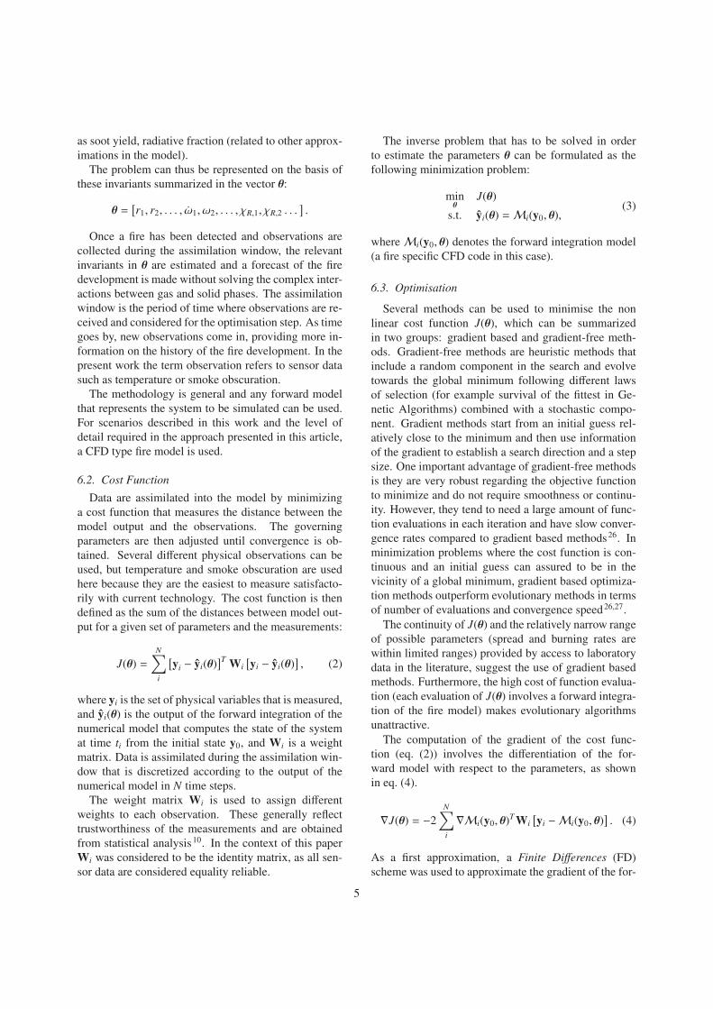
Figure 3 illustrates the inverse modelling process us-

ing the TLM approach. A scriptfile calls the forward

model (CFD) jobs (k + 1 in order to compute the k par-

tial derivatives for the gradient ofMi(y0, θ)), and, when

all of them have finished, calls the executable that com-

putes the TLM. Each CFD job provides an output file

with the data for the calculation of the gradient. These

files are read by the TLM executable, which then com-

putes θ by minimizing the TLM and provides a new set

of input files for the next iteration. The process is re-

peated until a user specified convergence criterion is met

(changes in the parameters from one iteration to the next

smaller than a threshold value).

An alternative to the TLM method for unconstrained

non-linear problems, the quasi-Newton Broyden-

Fletcher-Goldfarb-Shanno (BFGS) method is one of the

6

Figure 3: Inverse modelling procedure. The blue boxes

indicate processes executed by a script file. Red boxes

indicate the execution of the TLM method and its output

files. Green boxes are the fire model.

most widely used as it requires only first order derivative

computation, but conserves the good convergence char-

acteristics of the Newton method27. The BGFS method

is a Newton based optimization algorithm where the

second order derivatives are estimated from the first

order derivatives instead of calculating them directly.

In spite of being computationally less expensive than

the traditional Newton method, the computational ef-

fort of finding the optimum using the BFGS method is

still considerable, as more than one function evaluation

(model run) is required for each iteration in order to find

an adequate step size.

Both the TLM and the BGFS methods were imple-

mented in this work. It is shown in the results that TLM

has a superior performance for the problem at hand.

7. Results for a range of cases

7.1. Synthetic observations

The inverse problem procedure explained in the pre-

vious sections is illustrated applying it to a range of fire

cases. The CFD model used is the fire-specific LES

code Fire Dynamics Simulator version 5.1.6 (FDSv5)29.

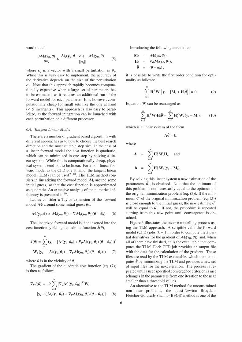
The test scenario consists of a compartment of 4m ×5m × 2.5m with a door on one side, and a window on

the opposite wall (see fig. 4). The fire is started at the

corner of a bed located in the room as shown in fig. 5. It

is then allowed to grow over the surface of the bed.

The observations used are synthetic data generated

using the same CFD model (FDSv5) with a set of pa-

rameter values that are referred to as true values. For

the spread rate, values reported in literature for real fires

typically range from 1 mm/s to 8 mm/s depending on

material and layout1. The range of possible values for

the fuel mass flow rate is from 10 to 50 g/m2s1. The ef-

fective heat of combustion Δhc of the fuel is a relatively

well defined quantity that depends mostly on the burn-

ing material and the combustion efficiency but varies

only slightly for similar fuels30, and thus, an average

value of 19 MJ/kg is used. It can be shown analyti-

cally that the HRR is most sensitive to the spread rate,

followed by the fuel mass flow rate and is relatively in-

sensitive to heat of combustion9. A grid size of 10 cm

is used, and the synthetic observations are generated for

300 s of fire.

(a)

(b)

Figure 4: Set up for the fire scenario; a) the computa-

tional domain with the fire compartment (view through

the door with the window on the opposite wall); b) the

same compartment with outlined walls. The thermocou-

ples in the ceiling are shown as dots.

The output of the CFD model, both for the forecast

and for the observations, consists of wall temperatures

7

measured with thermocouples in the ceiling and smoke

obscuration from wall-to-wall beam detectors.

Wall temperature sensors are distributed uniformly

on a rectangular grid throughout the ceiling, result-

ing in 99 sensor locations (approximate density of 5

sensors/m2) as shown in fig. 5. Eleven beam detectors

across the compartment, installed 10 cm below the ceil-

ing, provide smoke observation observations. The posi-

tion of the full set of sensors is shown in fig. 5, where the

blue lines represent the wall-to-wall laser beams cross-

ing the room. White noise is added to the observations

with a random, zero mean perturbation to the initial con-

ditions, in order to account for realistic perturbations ex-

pected in sensor data.

����

� � � � �

�����

� � � � �

�����

� � � � �

�����

���

�

���

� ����

�������������

�� ����������

��������

���������

��������

������� !�"�#$

�

���

Figure 5: Top view of the compartment. The green dots

represent the thermocouples in the ceiling, and the blue

lines are the beam detectors.

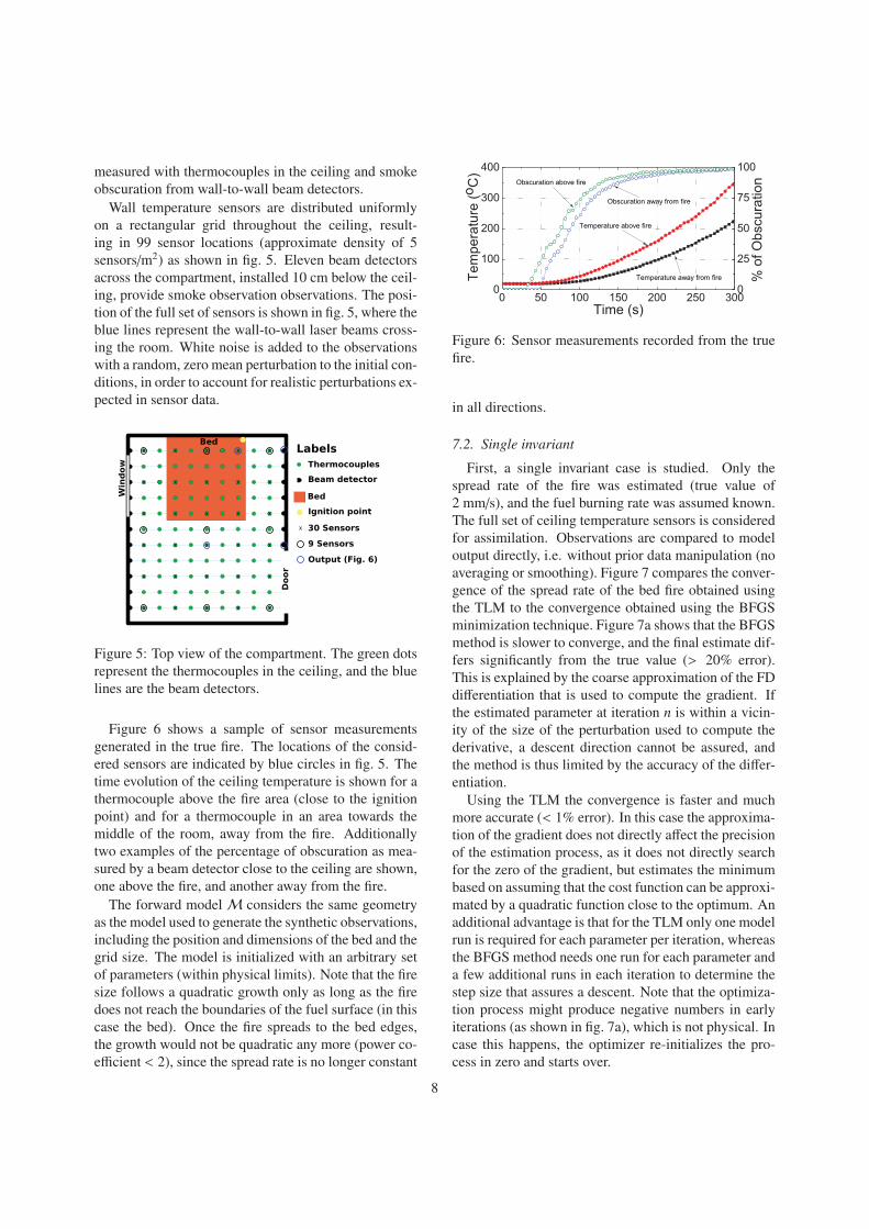
Figure 6 shows a sample of sensor measurements

generated in the true fire. The locations of the consid-

ered sensors are indicated by blue circles in fig. 5. The

time evolution of the ceiling temperature is shown for a

thermocouple above the fire area (close to the ignition

point) and for a thermocouple in an area towards the

middle of the room, away from the fire. Additionally

two examples of the percentage of obscuration as mea-

sured by a beam detector close to the ceiling are shown,

one above the fire, and another away from the fire.

The forward modelM considers the same geometry

as the model used to generate the synthetic observations,

including the position and dimensions of the bed and the

grid size. The model is initialized with an arbitrary set

of parameters (within physical limits). Note that the fire

size follows a quadratic growth only as long as the fire

does not reach the boundaries of the fuel surface (in this

case the bed). Once the fire spreads to the bed edges,

the growth would not be quadratic any more (power co-

efficient < 2), since the spread rate is no longer constant

� �� ��� ��� ��� ��� ����

���

���

���

���

����������� ����������

�������������

�������

������������� ����������

������������������

�

��

��

��

���

��������������

��������������������

Figure 6: Sensor measurements recorded from the true

fire.

in all directions.

7.2. Single invariant

First, a single invariant case is studied. Only the

spread rate of the fire was estimated (true value of

2 mm/s), and the fuel burning rate was assumed known.

The full set of ceiling temperature sensors is considered

for assimilation. Observations are compared to model

output directly, i.e. without prior data manipulation (no

averaging or smoothing). Figure 7 compares the conver-

gence of the spread rate of the bed fire obtained using

the TLM to the convergence obtained using the BFGS

minimization technique. Figure 7a shows that the BFGS

method is slower to converge, and the final estimate dif-

fers significantly from the true value (> 20% error).

This is explained by the coarse approximation of the FD

differentiation that is used to compute the gradient. If

the estimated parameter at iteration n is within a vicin-

ity of the size of the perturbation used to compute the

derivative, a descent direction cannot be assured, and

the method is thus limited by the accuracy of the differ-

entiation.

Using the TLM the convergence is faster and much

more accurate (< 1% error). In this case the approxima-

tion of the gradient does not directly affect the precision

of the estimation process, as it does not directly search

for the zero of the gradient, but estimates the minimum

based on assuming that the cost function can be approxi-

mated by a quadratic function close to the optimum. An

additional advantage is that for the TLM only one model

run is required for each parameter per iteration, whereas

the BFGS method needs one run for each parameter and

a few additional runs in each iteration to determine the

step size that assures a descent. Note that the optimiza-

tion process might produce negative numbers in early

iterations (as shown in fig. 7a), which is not physical. In

case this happens, the optimizer re-initializes the pro-

cess in zero and starts over.

8

� � �� �� �� �� ������

���

���

���

��

����

��������

������ �

���������

����������

�� ���������� ������

(a)

� � � � �

�

��

���

�����������

���������

(b)

Figure 7: Comparison of TLM and BFGS for a single

invariant problem; (a) shows the spread rate estimated

at different iterations, and (b) shows the convergence of

the error between the estimations and the true values.

Given the superior performance of the TLM, both in

accuracy and in computation time, it was decided to

concentrate on the TLM and not to develop the BFGS

method for multi-parameter estimation.

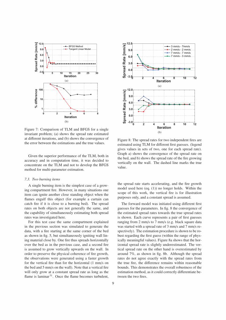
7.3. Two burning items

A single burning item is the simplest case of a grow-

ing compartment fire. However, in many situations one

item can ignite another close standing object when the

flames engulf this object (for example a curtain can

catch fire if it is close to a burning bed). The spread

rates on both objects are not generally the same, and

the capability of simultaneously estimating both spread

rates was investigated here.

For this test case the same compartment explained

in the previous section was simulated to generate the

data, with a fire starting at the same corner of the bed

as shown in fig. 5, but simultaneously igniting wall lin-

ing material close by. One fire thus spreads horizontally

over the bed as in the previous case, and a second fire

is assumed to grow vertically upwards on the wall. In

order to preserve the physical coherence of fire growth,

the observations were generated using a faster growth

for the vertical fire than for the horizontal (1 mm/s on

the bed and 5 mm/s on the wall). Note that a vertical fire

will only grow at a constant spread rate as long as the

flame is laminar31. Once the flame becomes turbulent,

� � � � � �� �����

��

��

��

�

���

��������

������ �

���������

���������������

����������������

����������������

����������������

(a)

� � � � � �� �����

��

��

��

�

���

��������

������ �

���������

(b)

Figure 8: The spread rates for two independent fires are

estimated using TLM for different first guesses. (legend

gives values in sets of two, one for each spread rate).

Graph a) shows the convergence of the spread rate on

the bed, and b) shows the spread rate of the fire growing

vertically on the wall. The dashed line marks the true

value.

the spread rate starts accelerating, and the fire growth

model used here (eq. (1)) no longer holds. Within the

scope of this work, the vertical fire is for illustration

purposes only, and a constant spread is assumed.

The forward model was initiated using different first

guesses for the parameters. In fig. 8 the convergence of

the estimated spread rates towards the true spread rates

is shown. Each curve represents a pair of first guesses

ranging from 2 mm/s to 7 mm/s (e.g. black square data

was started with a spread rate of 3 mm/s and 7 mm/s re-

spectively). The estimation procedure is shown to be ro-

bust regarding the first guess (within the range of phys-

ically meaningful values). Figure 8a shows that the hor-

izontal spread rate is slightly underestimated. The ver-

tical spread rate on the other hand is overestimated by

around 7%, as shown in fig. 8b. Although the spread

rates do not agree exactly with the spread rates from

the true fire, the difference remains within reasonable

bounds. This demonstrates the overall robustness of the

estimation method, as it could correctly differentiate be-

tween the two fires.

9

� � � � � �� �����

���

���

���

���

��

���

��������

������ �

���������

(a)

� � � � � �� ������

����

����

����

����

���

����

���������������������

��

������������������� ��

� ����������������� ��

������������������� ��

������������������� ��

������������� �

��

���������

(b)

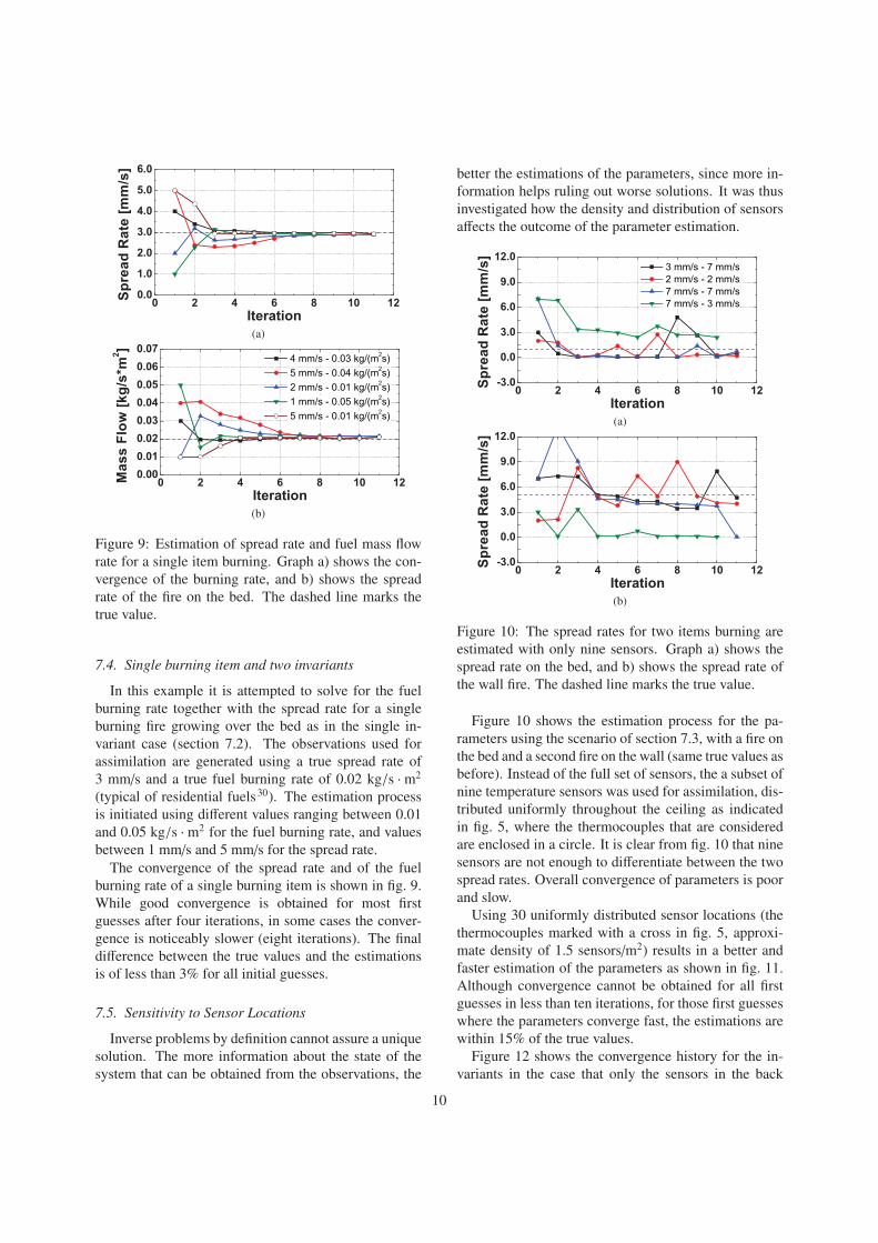
Figure 9: Estimation of spread rate and fuel mass flow

rate for a single item burning. Graph a) shows the con-

vergence of the burning rate, and b) shows the spread

rate of the fire on the bed. The dashed line marks the

true value.

7.4. Single burning item and two invariants

In this example it is attempted to solve for the fuel

burning rate together with the spread rate for a single

burning fire growing over the bed as in the single in-

variant case (section 7.2). The observations used for

assimilation are generated using a true spread rate of

3 mm/s and a true fuel burning rate of 0.02 kg/s ·m2

(typical of residential fuels30). The estimation process

is initiated using different values ranging between 0.01

and 0.05 kg/s ·m2 for the fuel burning rate, and values

between 1 mm/s and 5 mm/s for the spread rate.

The convergence of the spread rate and of the fuel

burning rate of a single burning item is shown in fig. 9.

While good convergence is obtained for most first

guesses after four iterations, in some cases the conver-

gence is noticeably slower (eight iterations). The final

difference between the true values and the estimations

is of less than 3% for all initial guesses.

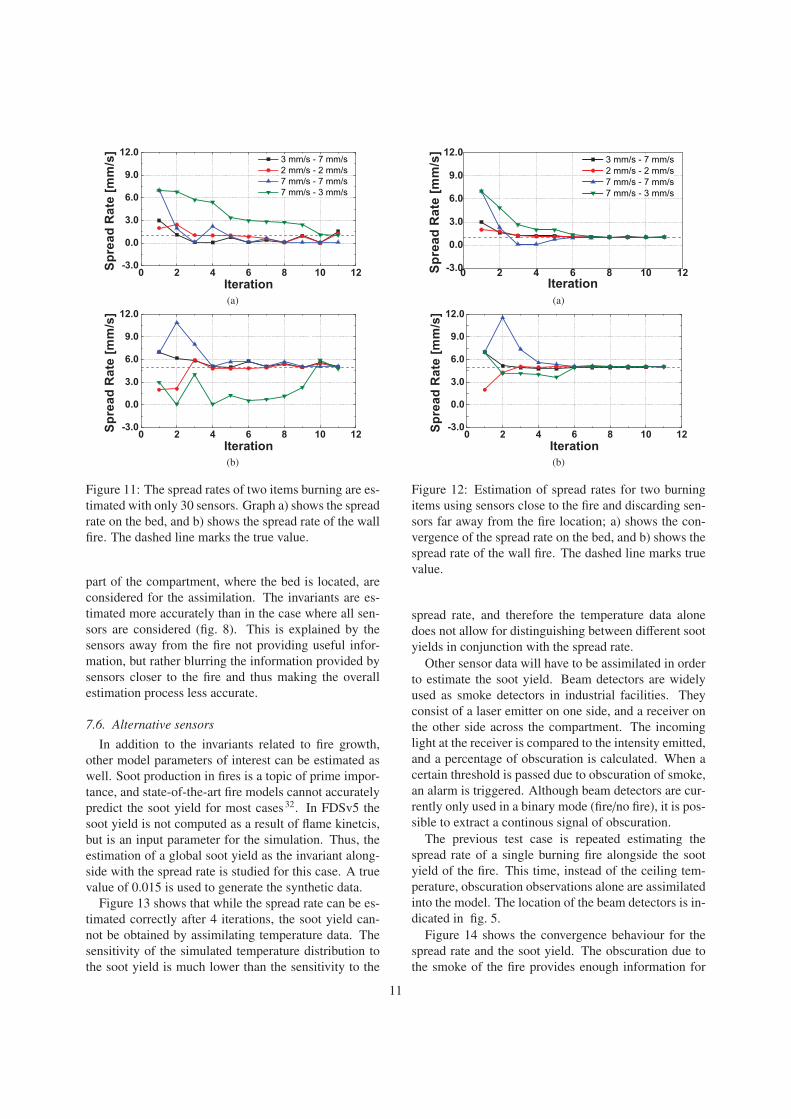
7.5. Sensitivity to Sensor Locations

Inverse problems by definition cannot assure a unique

solution. The more information about the state of the

system that can be obtained from the observations, the

better the estimations of the parameters, since more in-

formation helps ruling out worse solutions. It was thus

investigated how the density and distribution of sensors

affects the outcome of the parameter estimation.

� � � � � �� �����

��

��

��

�

���

��������

������ �

���������

����������������

����������������

����������������

����������������

(a)

� � � � � �� �����

��

��

��

�

���

��������

������ �

���������

(b)

Figure 10: The spread rates for two items burning are

estimated with only nine sensors. Graph a) shows the

spread rate on the bed, and b) shows the spread rate of

the wall fire. The dashed line marks the true value.

Figure 10 shows the estimation process for the pa-

rameters using the scenario of section 7.3, with a fire on

the bed and a second fire on the wall (same true values as

before). Instead of the full set of sensors, the a subset of

nine temperature sensors was used for assimilation, dis-

tributed uniformly throughout the ceiling as indicated

in fig. 5, where the thermocouples that are considered

are enclosed in a circle. It is clear from fig. 10 that nine

sensors are not enough to differentiate between the two

spread rates. Overall convergence of parameters is poor

and slow.

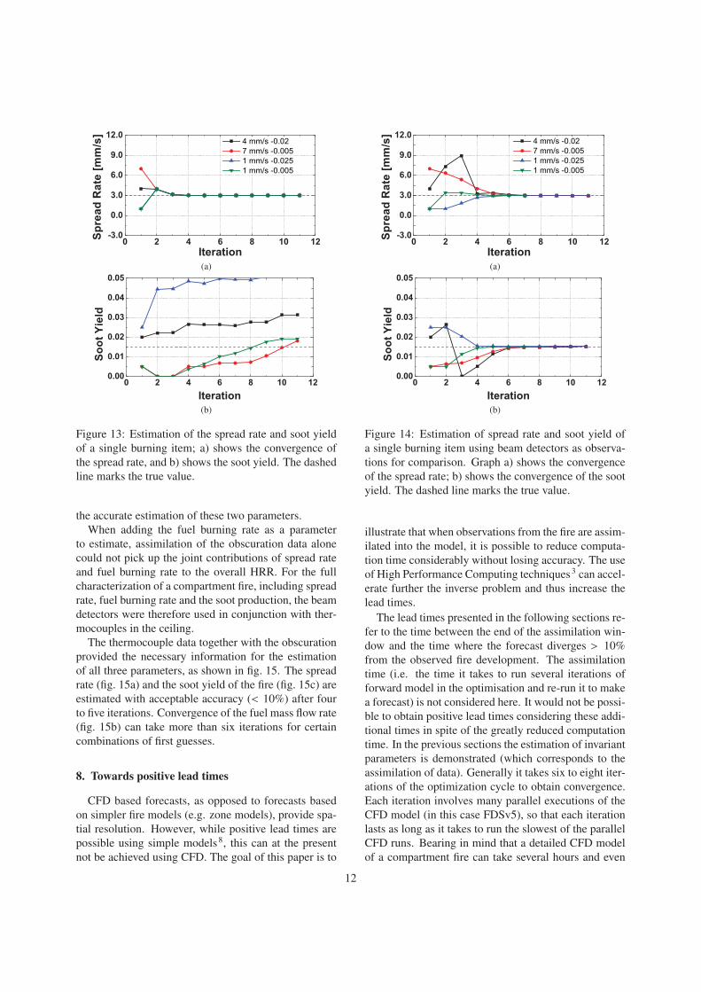
Using 30 uniformly distributed sensor locations (the

thermocouples marked with a cross in fig. 5, approxi-

mate density of 1.5 sensors/m2) results in a better and

faster estimation of the parameters as shown in fig. 11.

Although convergence cannot be obtained for all first

guesses in less than ten iterations, for those first guesses

where the parameters converge fast, the estimations are

within 15% of the true values.

Figure 12 shows the convergence history for the in-

variants in the case that only the sensors in the back

10

� � � � � �� �����

��

��

��

�

���

��������

������ �

���������

����������������

����������������

����������������

����������������

(a)

� � � � � �� �����

��

��

��

�

���

��������

������ �

���������

(b)

Figure 11: The spread rates of two items burning are es-

timated with only 30 sensors. Graph a) shows the spread

rate on the bed, and b) shows the spread rate of the wall

fire. The dashed line marks the true value.

part of the compartment, where the bed is located, are

considered for the assimilation. The invariants are es-

timated more accurately than in the case where all sen-

sors are considered (fig. 8). This is explained by the

sensors away from the fire not providing useful infor-

mation, but rather blurring the information provided by

sensors closer to the fire and thus making the overall

estimation process less accurate.

7.6. Alternative sensorsIn addition to the invariants related to fire growth,

other model parameters of interest can be estimated as

well. Soot production in fires is a topic of prime impor-

tance, and state-of-the-art fire models cannot accurately

predict the soot yield for most cases32. In FDSv5 the

soot yield is not computed as a result of flame kinetcis,

but is an input parameter for the simulation. Thus, the

estimation of a global soot yield as the invariant along-

side with the spread rate is studied for this case. A true

value of 0.015 is used to generate the synthetic data.

Figure 13 shows that while the spread rate can be es-

timated correctly after 4 iterations, the soot yield can-

not be obtained by assimilating temperature data. The

sensitivity of the simulated temperature distribution to

the soot yield is much lower than the sensitivity to the

� � � � � �� �����

��

��

��

�

���

��������

������ �

���������

����������������

����������������

����������������

����������������

(a)

� � � � � �� �����

��

��

��

�

���

��������

������ �

���������

(b)

Figure 12: Estimation of spread rates for two burning

items using sensors close to the fire and discarding sen-

sors far away from the fire location; a) shows the con-

vergence of the spread rate on the bed, and b) shows the

spread rate of the wall fire. The dashed line marks true

value.

spread rate, and therefore the temperature data alone

does not allow for distinguishing between different soot

yields in conjunction with the spread rate.

Other sensor data will have to be assimilated in order

to estimate the soot yield. Beam detectors are widely

used as smoke detectors in industrial facilities. They

consist of a laser emitter on one side, and a receiver on

the other side across the compartment. The incoming

light at the receiver is compared to the intensity emitted,

and a percentage of obscuration is calculated. When a

certain threshold is passed due to obscuration of smoke,

an alarm is triggered. Although beam detectors are cur-

rently only used in a binary mode (fire/no fire), it is pos-

sible to extract a continous signal of obscuration.

The previous test case is repeated estimating the

spread rate of a single burning fire alongside the soot

yield of the fire. This time, instead of the ceiling tem-

perature, obscuration observations alone are assimilated

into the model. The location of the beam detectors is in-

dicated in fig. 5.

Figure 14 shows the convergence behaviour for the

spread rate and the soot yield. The obscuration due to

the smoke of the fire provides enough information for

11

� � � � � �� �����

��

��

��

�

���

��������

������ �

���������

������������

�������������

�������������

��������������

(a)

� � � � � �� ������

����

����

����

����

���

���������

���������

(b)

Figure 13: Estimation of the spread rate and soot yield

of a single burning item; a) shows the convergence of

the spread rate, and b) shows the soot yield. The dashed

line marks the true value.

the accurate estimation of these two parameters.

When adding the fuel burning rate as a parameter

to estimate, assimilation of the obscuration data alone

could not pick up the joint contributions of spread rate

and fuel burning rate to the overall HRR. For the full

characterization of a compartment fire, including spread

rate, fuel burning rate and the soot production, the beam

detectors were therefore used in conjunction with ther-

mocouples in the ceiling.

The thermocouple data together with the obscuration

provided the necessary information for the estimation

of all three parameters, as shown in fig. 15. The spread

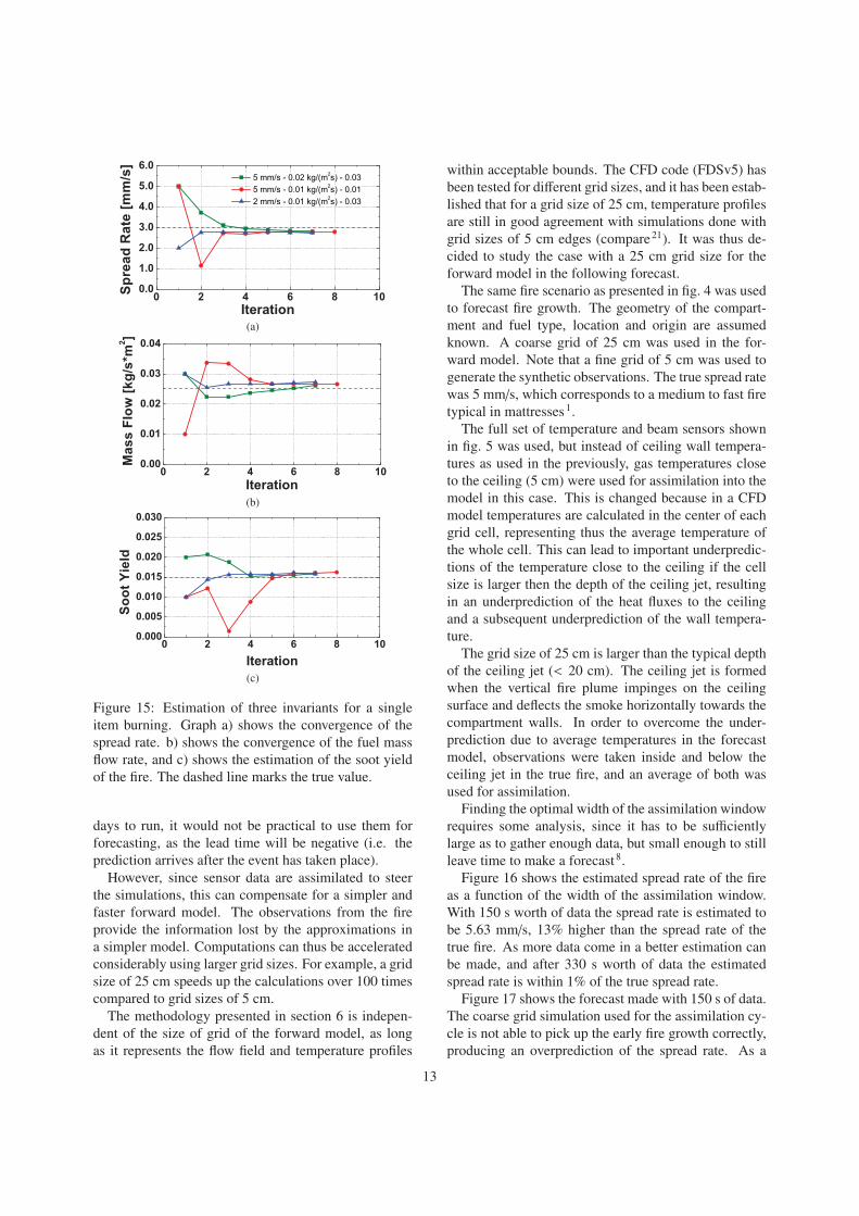
rate (fig. 15a) and the soot yield of the fire (fig. 15c) are

estimated with acceptable accuracy (< 10%) after four

to five iterations. Convergence of the fuel mass flow rate

(fig. 15b) can take more than six iterations for certain

combinations of first guesses.

8. Towards positive lead times

CFD based forecasts, as opposed to forecasts based

on simpler fire models (e.g. zone models), provide spa-

tial resolution. However, while positive lead times are

possible using simple models8, this can at the present

not be achieved using CFD. The goal of this paper is to

� � � � � �� �����

��

��

��

�

���

��������

������ �

���������

������������

�������������

�������������

��������������

(a)

� � � � � �� ������

����

����

����

����

���

���������

���������

(b)

Figure 14: Estimation of spread rate and soot yield of

a single burning item using beam detectors as observa-

tions for comparison. Graph a) shows the convergence

of the spread rate; b) shows the convergence of the soot

yield. The dashed line marks the true value.

illustrate that when observations from the fire are assim-

ilated into the model, it is possible to reduce computa-

tion time considerably without losing accuracy. The use

of High Performance Computing techniques3 can accel-

erate further the inverse problem and thus increase the

lead times.

The lead times presented in the following sections re-

fer to the time between the end of the assimilation win-

dow and the time where the forecast diverges > 10%

from the observed fire development. The assimilation

time (i.e. the time it takes to run several iterations of

forward model in the optimisation and re-run it to make

a forecast) is not considered here. It would not be possi-

ble to obtain positive lead times considering these addi-

tional times in spite of the greatly reduced computation

time. In the previous sections the estimation of invariant

parameters is demonstrated (which corresponds to the

assimilation of data). Generally it takes six to eight iter-

ations of the optimization cycle to obtain convergence.

Each iteration involves many parallel executions of the

CFD model (in this case FDSv5), so that each iteration

lasts as long as it takes to run the slowest of the parallel

CFD runs. Bearing in mind that a detailed CFD model

of a compartment fire can take several hours and even

12

� � � � � �����

���

���

���

���

��

���

��������

������ �

���������

������������������� �������

�������������������� �������

������������������� �������

(a)

� � � � � ������

����

����

����

����

������������� �

��

���������

(b)

� � � � � �������

�����

�����

�����

�����

�����

����

���������

���������

(c)

Figure 15: Estimation of three invariants for a single

item burning. Graph a) shows the convergence of the

spread rate. b) shows the convergence of the fuel mass

flow rate, and c) shows the estimation of the soot yield

of the fire. The dashed line marks the true value.

days to run, it would not be practical to use them for

forecasting, as the lead time will be negative (i.e. the

prediction arrives after the event has taken place).

However, since sensor data are assimilated to steer

the simulations, this can compensate for a simpler and

faster forward model. The observations from the fire

provide the information lost by the approximations in

a simpler model. Computations can thus be accelerated

considerably using larger grid sizes. For example, a grid

size of 25 cm speeds up the calculations over 100 times

compared to grid sizes of 5 cm.

The methodology presented in section 6 is indepen-

dent of the size of grid of the forward model, as long

as it represents the flow field and temperature profiles

within acceptable bounds. The CFD code (FDSv5) has

been tested for different grid sizes, and it has been estab-

lished that for a grid size of 25 cm, temperature profiles

are still in good agreement with simulations done with

grid sizes of 5 cm edges (compare21). It was thus de-

cided to study the case with a 25 cm grid size for the

forward model in the following forecast.

The same fire scenario as presented in fig. 4 was used

to forecast fire growth. The geometry of the compart-

ment and fuel type, location and origin are assumed

known. A coarse grid of 25 cm was used in the for-

ward model. Note that a fine grid of 5 cm was used to

generate the synthetic observations. The true spread rate

was 5 mm/s, which corresponds to a medium to fast fire

typical in mattresses1.

The full set of temperature and beam sensors shown

in fig. 5 was used, but instead of ceiling wall tempera-

tures as used in the previously, gas temperatures close

to the ceiling (5 cm) were used for assimilation into the

model in this case. This is changed because in a CFD

model temperatures are calculated in the center of each

grid cell, representing thus the average temperature of

the whole cell. This can lead to important underpredic-

tions of the temperature close to the ceiling if the cell

size is larger then the depth of the ceiling jet, resulting

in an underprediction of the heat fluxes to the ceiling

and a subsequent underprediction of the wall tempera-

ture.

The grid size of 25 cm is larger than the typical depth

of the ceiling jet (< 20 cm). The ceiling jet is formed

when the vertical fire plume impinges on the ceiling

surface and deflects the smoke horizontally towards the

compartment walls. In order to overcome the under-

prediction due to average temperatures in the forecast

model, observations were taken inside and below the

ceiling jet in the true fire, and an average of both was

used for assimilation.

Finding the optimal width of the assimilation window

requires some analysis, since it has to be sufficiently

large as to gather enough data, but small enough to still

leave time to make a forecast8.

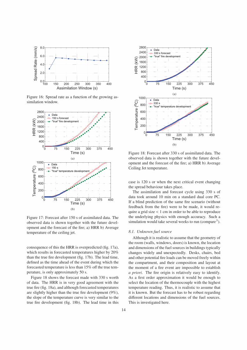
Figure 16 shows the estimated spread rate of the fire

as a function of the width of the assimilation window.

With 150 s worth of data the spread rate is estimated to

be 5.63 mm/s, 13% higher than the spread rate of the

true fire. As more data come in a better estimation can

be made, and after 330 s worth of data the estimated

spread rate is within 1% of the true spread rate.

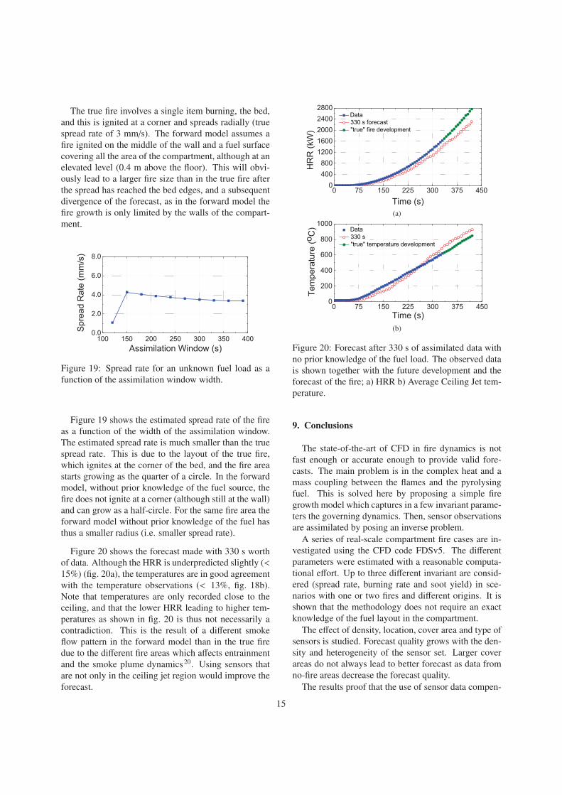
Figure 17 shows the forecast made with 150 s of data.

The coarse grid simulation used for the assimilation cy-

cle is not able to pick up the early fire growth correctly,

producing an overprediction of the spread rate. As a

13

��� ��� ��� ��� ��� ��� ������

���

���

���

��

��������

������ �

�������������� ����

Figure 16: Spread rate as a function of the growing as-

similation window.

� �� ��� ��� ��� ��� ����

���

���

����

���

����

����

�����

��������

��������

��

�� �����������

������������������������

(a)

� �� ��� ��� ��� ��� ����

���

���

���

��

����

�

�������������

��������

��

�� ���

������������������������������

(b)

Figure 17: Forecast after 150 s of assimilated data. The

observed data is shown together with the future devel-

opment and the forecast of the fire; a) HRR b) Average

temperature of the ceiling jet.

consequence of this the HRR is overpredicted (fig. 17a),

which results in forecasted temperatures higher by 20%

than the true fire development (fig. 17b). The lead time,

defined as the time ahead of the event during which the

forecasted temperature is less than 15% off the true tem-

perature, is only approximately 50 s.

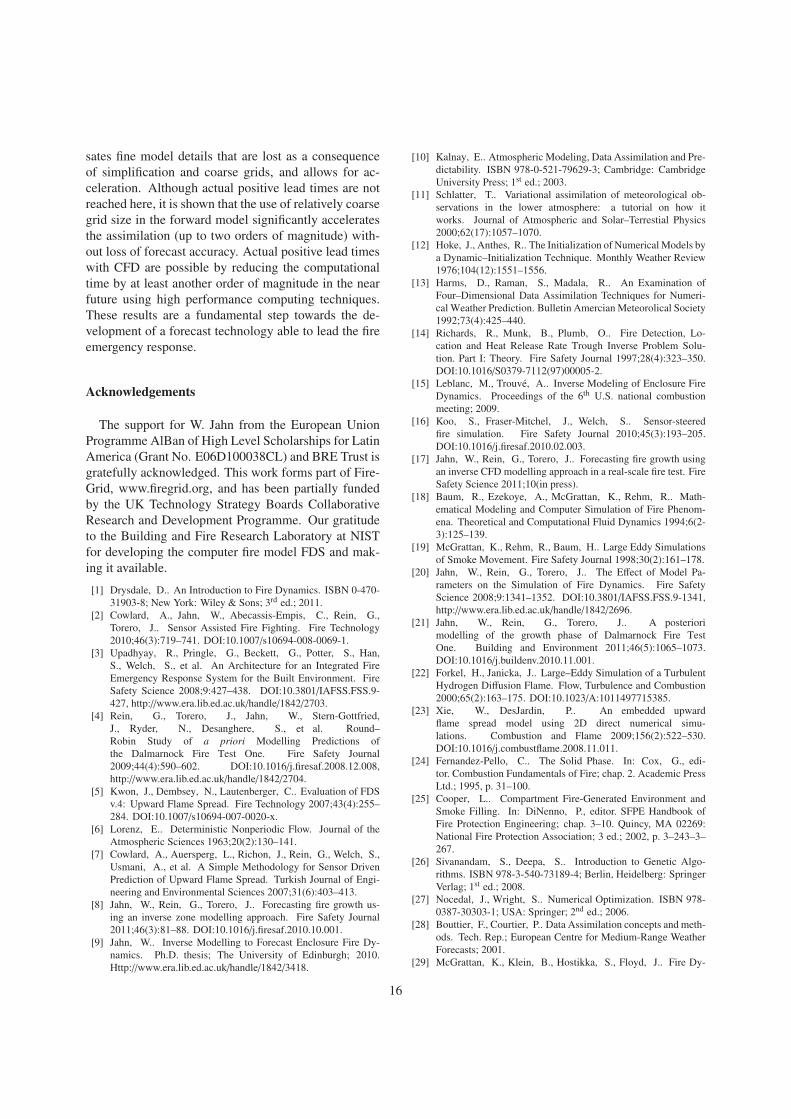
Figure 18 shows the forecast made with 330 s worth

of data. The HRR is in very good agreement with the

true fire (fig. 18a), and although forecasted temperatures

are slightly higher than the true fire development (9%),

the slope of the temperature curve is very similar to the

true fire development (fig. 18b). The lead time in this

� �� ��� ��� ��� ��� ����

���

���

����

���

����

����

����

��������

��������

��

��� ����������

������������������������

(a)

� �� ��� ��� ��� ��� ����

���

���

���

��

����

�������������

��������

��

��� ��

������������������������������

(b)

Figure 18: Forecast after 330 s of assimilated data. The

observed data is shown together with the future devel-

opment and the forecast of the fire; a) HRR b) Average

Ceiling Jet temperature.

case is 120 s or when the next critical event changing

the spread behaviour takes place.

The assimilation and forecast cycle using 330 s of

data took around 10 min on a standard dual core PC.

If a blind prediction of the same fire scenario (without

feedback from the fire) were to be made, it would re-

quire a grid size < 1 cm in order to be able to reproduce

the underlying physics with enough accuracy. Such a

simulation would take several weeks to run (compare5).

8.1. Unknown fuel sourceAlthough it is realistic to assume that the geometry of

the room (walls, windows, doors) is known, the location

and dimensions of the fuel sources in buildings typically

changes widely and unexpectedly. Desks, chairs, bed

and other potential fire loads can be moved freely within

the compartment, and their composition and layout at

the moment of a fire event are impossible to establish

a priori. The fire origin is relatively easy to identify.

As a first order approximation it would be enough to

select the location of the thermocouple with the highest

temperature reading. Thus, it is realistic to assume that

it is known. But the forecast has to be robust regarding

different locations and dimensions of the fuel sources.

This is investigated here.

14

The true fire involves a single item burning, the bed,

and this is ignited at a corner and spreads radially (true

spread rate of 3 mm/s). The forward model assumes a

fire ignited on the middle of the wall and a fuel surface

covering all the area of the compartment, although at an

elevated level (0.4 m above the floor). This will obvi-

ously lead to a larger fire size than in the true fire after

the spread has reached the bed edges, and a subsequent

divergence of the forecast, as in the forward model the

fire growth is only limited by the walls of the compart-

ment.

��� ��� ��� ��� ��� ��� ������

���

���

���

��

��������

������ �

��������������� ���

Figure 19: Spread rate for an unknown fuel load as a

function of the assimilation window width.

Figure 19 shows the estimated spread rate of the fire

as a function of the width of the assimilation window.

The estimated spread rate is much smaller than the true

spread rate. This is due to the layout of the true fire,

which ignites at the corner of the bed, and the fire area

starts growing as the quarter of a circle. In the forward

model, without prior knowledge of the fuel source, the

fire does not ignite at a corner (although still at the wall)

and can grow as a half-circle. For the same fire area the

forward model without prior knowledge of the fuel has

thus a smaller radius (i.e. smaller spread rate).

Figure 20 shows the forecast made with 330 s worth

of data. Although the HRR is underpredicted slightly (<15%) (fig. 20a), the temperatures are in good agreement

with the temperature observations (< 13%, fig. 18b).

Note that temperatures are only recorded close to the

ceiling, and that the lower HRR leading to higher tem-

peratures as shown in fig. 20 is thus not necessarily a

contradiction. This is the result of a different smoke

flow pattern in the forward model than in the true fire

due to the different fire areas which affects entrainment

and the smoke plume dynamics20. Using sensors that

are not only in the ceiling jet region would improve the

forecast.

� �� ��� ��� ��� ��� ����

���

���

����

���

����

����

����

��������

��������

��

��� ����������

������������������������

(a)

� �� ��� ��� ��� ��� ����

���

���

���

��

����

�������������

��������

��

��� ��

������������������������������

(b)

Figure 20: Forecast after 330 s of assimilated data with

no prior knowledge of the fuel load. The observed data

is shown together with the future development and the

forecast of the fire; a) HRR b) Average Ceiling Jet tem-

perature.

9. Conclusions

The state-of-the-art of CFD in fire dynamics is not

fast enough or accurate enough to provide valid fore-

casts. The main problem is in the complex heat and a

mass coupling between the flames and the pyrolysing

fuel. This is solved here by proposing a simple fire

growth model which captures in a few invariant parame-

ters the governing dynamics. Then, sensor observations

are assimilated by posing an inverse problem.

A series of real-scale compartment fire cases are in-

vestigated using the CFD code FDSv5. The different

parameters were estimated with a reasonable computa-

tional effort. Up to three different invariant are consid-

ered (spread rate, burning rate and soot yield) in sce-

narios with one or two fires and different origins. It is

shown that the methodology does not require an exact

knowledge of the fuel layout in the compartment.

The effect of density, location, cover area and type of

sensors is studied. Forecast quality grows with the den-

sity and heterogeneity of the sensor set. Larger cover

areas do not always lead to better forecast as data from

no-fire areas decrease the forecast quality.

The results proof that the use of sensor data compen-

15

sates fine model details that are lost as a consequence

of simplification and coarse grids, and allows for ac-

celeration. Although actual positive lead times are not

reached here, it is shown that the use of relatively coarse

grid size in the forward model significantly accelerates

the assimilation (up to two orders of magnitude) with-

out loss of forecast accuracy. Actual positive lead times

with CFD are possible by reducing the computational

time by at least another order of magnitude in the near

future using high performance computing techniques.

These results are a fundamental step towards the de-

velopment of a forecast technology able to lead the fire

emergency response.

Acknowledgements

The support for W. Jahn from the European Union

Programme AlBan of High Level Scholarships for Latin

America (Grant No. E06D100038CL) and BRE Trust is

gratefully acknowledged. This work forms part of Fire-

Grid, www.firegrid.org, and has been partially funded

by the UK Technology Strategy Boards Collaborative

Research and Development Programme. Our gratitude

to the Building and Fire Research Laboratory at NIST

for developing the computer fire model FDS and mak-

ing it available.

[1] Drysdale, D.. An Introduction to Fire Dynamics. ISBN 0-470-

31903-8; New York: Wiley & Sons; 3rd ed.; 2011.

[2] Cowlard, A., Jahn, W., Abecassis-Empis, C., Rein, G.,

Torero, J.. Sensor Assisted Fire Fighting. Fire Technology

2010;46(3):719–741. DOI:10.1007/s10694-008-0069-1.

[3] Upadhyay, R., Pringle, G., Beckett, G., Potter, S., Han,

S., Welch, S., et al. An Architecture for an Integrated Fire

Emergency Response System for the Built Environment. Fire

Safety Science 2008;9:427–438. DOI:10.3801/IAFSS.FSS.9-

427, http://www.era.lib.ed.ac.uk/handle/1842/2703.

[4] Rein, G., Torero, J., Jahn, W., Stern-Gottfried,

J., Ryder, N., Desanghere, S., et al. Round–

Robin Study of a priori Modelling Predictions of

the Dalmarnock Fire Test One. Fire Safety Journal

2009;44(4):590–602. DOI:10.1016/j.firesaf.2008.12.008,

http://www.era.lib.ed.ac.uk/handle/1842/2704.

[5] Kwon, J., Dembsey, N., Lautenberger, C.. Evaluation of FDS

v.4: Upward Flame Spread. Fire Technology 2007;43(4):255–

284. DOI:10.1007/s10694-007-0020-x.

[6] Lorenz, E.. Deterministic Nonperiodic Flow. Journal of the

Atmospheric Sciences 1963;20(2):130–141.

[7] Cowlard, A., Auersperg, L., Richon, J., Rein, G., Welch, S.,

Usmani, A., et al. A Simple Methodology for Sensor Driven

Prediction of Upward Flame Spread. Turkish Journal of Engi-

neering and Environmental Sciences 2007;31(6):403–413.

[8] Jahn, W., Rein, G., Torero, J.. Forecasting fire growth us-

ing an inverse zone modelling approach. Fire Safety Journal

2011;46(3):81–88. DOI:10.1016/j.firesaf.2010.10.001.

[9] Jahn, W.. Inverse Modelling to Forecast Enclosure Fire Dy-

namics. Ph.D. thesis; The University of Edinburgh; 2010.

Http://www.era.lib.ed.ac.uk/handle/1842/3418.

[10] Kalnay, E.. Atmospheric Modeling, Data Assimilation and Pre-

dictability. ISBN 978-0-521-79629-3; Cambridge: Cambridge

University Press; 1st ed.; 2003.

[11] Schlatter, T.. Variational assimilation of meteorological ob-

servations in the lower atmosphere: a tutorial on how it

works. Journal of Atmospheric and Solar–Terrestial Physics

2000;62(17):1057–1070.

[12] Hoke, J., Anthes, R.. The Initialization of Numerical Models by

a Dynamic–Initialization Technique. Monthly Weather Review

1976;104(12):1551–1556.

[13] Harms, D., Raman, S., Madala, R.. An Examination of

Four–Dimensional Data Assimilation Techniques for Numeri-

cal Weather Prediction. Bulletin Amercian Meteorolical Society

1992;73(4):425–440.

[14] Richards, R., Munk, B., Plumb, O.. Fire Detection, Lo-

cation and Heat Release Rate Trough Inverse Problem Solu-

tion. Part I: Theory. Fire Safety Journal 1997;28(4):323–350.

DOI:10.1016/S0379-7112(97)00005-2.

[15] Leblanc, M., Trouve, A.. Inverse Modeling of Enclosure Fire

Dynamics. Proceedings of the 6th U.S. national combustion

meeting; 2009.

[16] Koo, S., Fraser-Mitchel, J., Welch, S.. Sensor-steered

fire simulation. Fire Safety Journal 2010;45(3):193–205.

DOI:10.1016/j.firesaf.2010.02.003.

[17] Jahn, W., Rein, G., Torero, J.. Forecasting fire growth using

an inverse CFD modelling approach in a real-scale fire test. Fire

Safety Science 2011;10(in press).

[18] Baum, R., Ezekoye, A., McGrattan, K., Rehm, R.. Math-

ematical Modeling and Computer Simulation of Fire Phenom-

ena. Theoretical and Computational Fluid Dynamics 1994;6(2-

3):125–139.

[19] McGrattan, K., Rehm, R., Baum, H.. Large Eddy Simulations

of Smoke Movement. Fire Safety Journal 1998;30(2):161–178.

[20] Jahn, W., Rein, G., Torero, J.. The Effect of Model Pa-

rameters on the Simulation of Fire Dynamics. Fire Safety

Science 2008;9:1341–1352. DOI:10.3801/IAFSS.FSS.9-1341,

http://www.era.lib.ed.ac.uk/handle/1842/2696.

[21] Jahn, W., Rein, G., Torero, J.. A posteriori

modelling of the growth phase of Dalmarnock Fire Test

One. Building and Environment 2011;46(5):1065–1073.

DOI:10.1016/j.buildenv.2010.11.001.

[22] Forkel, H., Janicka, J.. Large–Eddy Simulation of a Turbulent

Hydrogen Diffusion Flame. Flow, Turbulence and Combustion

2000;65(2):163–175. DOI:10.1023/A:1011497715385.

[23] Xie, W., DesJardin, P.. An embedded upward

flame spread model using 2D direct numerical simu-

lations. Combustion and Flame 2009;156(2):522–530.

DOI:10.1016/j.combustflame.2008.11.011.

[24] Fernandez-Pello, C.. The Solid Phase. In: Cox, G., edi-

tor. Combustion Fundamentals of Fire; chap. 2. Academic Press

Ltd.; 1995, p. 31–100.

[25] Cooper, L.. Compartment Fire-Generated Environment and

Smoke Filling. In: DiNenno, P., editor. SFPE Handbook of

Fire Protection Engineering; chap. 3–10. Quincy, MA 02269:

National Fire Protection Association; 3 ed.; 2002, p. 3–243–3–

267.

[26] Sivanandam, S., Deepa, S.. Introduction to Genetic Algo-

rithms. ISBN 978-3-540-73189-4; Berlin, Heidelberg: Springer

Verlag; 1st ed.; 2008.

[27] Nocedal, J., Wright, S.. Numerical Optimization. ISBN 978-

0387-30303-1; USA: Springer; 2nd ed.; 2006.

[28] Bouttier, F., Courtier, P.. Data Assimilation concepts and meth-

ods. Tech. Rep.; European Centre for Medium-Range Weather

Forecasts; 2001.

[29] McGrattan, K., Klein, B., Hostikka, S., Floyd, J.. Fire Dy-

16

namics Simulator (Version 5) – User’s Guide. NIST Special

Publication 1019–5; 2008.

[30] Babrauskas, V.. Heat Release Rates. In: DiNenno, P., edi-

tor. SFPE Handbook of Fire Protection Engineering; chap. 3-1.

Quincy, MA 02269: National Fire Protection Association; 3 ed.;

2002, p. 3–1–3–37.

[31] Cowlard, A.. Sensor and Model Integration for the

Rapid Prediction of Concurrent Flow Flame Spread.

Ph.D. thesis; The University of Edinburgh; 2009.

Http://www.era.lib.ed.ac.uk/handle/1842/2753.

[32] Moss, J., Stewart, C., Young, K.. Modelling Soot For-

mation and Burnout in a High Temperature Laminar Diffu-

sion Flame Buning under Oxygen-Enriched Conditions. Com-

bustion and Flame 1995;101(4):491–500. DOI:10.1016/0010-

2180(94)00233-I.

17