Learning Inverse Dynamics for RobotManipulator Control

by

Joseph Sun de la Cruz

A thesispresented to the University of Waterloo

in fulfillment of thethesis requirement for the degree of

Master of Applied Sciencein

Electrical and Computer Engineering

Waterloo, Ontario, Canada, 2011

c© Joseph Sun de la Cruz 2011

I hereby declare that I am the sole author of this thesis. This is a true copy of the thesis,including any required final revisions, as accepted by my examiners.

I understand that my thesis may be made electronically available to the public.

ii

Abstract

Model-based control strategies for robot manipulators can present numerous perfor-mance advantages when an accurate model of the system dynamics is available. In practice,obtaining such a model is a challenging task which involves modeling such physical pro-cesses as friction, which may not be well understood and difficult to model. Furthermore,uncertainties in the physical parameters of a system may be introduced from significant dis-crepancies between the manufacturer data and the actual system. Traditionally, adaptiveand robust control strategies have been developed to deal with parametric uncertainty inthe dynamic model, but often require knowledge of the structure of the dynamics. Recentapproaches to model-based manipulator control involve data-driven learning of the inversedynamics relationship, eliminating the need for any a-priori knowledge of the system model.Locally Weighted Projection Regression (LWPR) has been proposed for learning the inversedynamics function of a manipulator. Due to its use of simple local, linear models, LWPRis suitable for online and incremental learning. Although global regression techniques suchas Gaussian Process Regression (GPR) have been shown to outperform LWPR in terms ofaccuracy, due to its heavy computational requirements, GPR has been applied mainly tooffline learning of inverse dynamics. More recent efforts in making GPR computationallytractable for real-time control have resulted in several approximations which operate on aselect subset, or sparse representation of the entire training data set.

Despite the significant advancements that have been made in the area of learning con-trol, there has not been much work in recent years to evaluate these newer regression tech-niques against traditional model-based control strategies such as adaptive control. Hence,the first portion of this thesis provides a comparison between a fixed model-based controlstrategy, an adaptive controller and the LWPR-based learning controller. Simulations arecarried out in order to evaluate the position and orientation tracking performance of eachcontroller under varied end effector loading, velocities and inaccuracies in the known dy-namic parameters. Both the adaptive controller and LWPR controller are shown to havecomparable performance in the presence of parametric uncertainty. However, it is shownthat the learning controller is unable to generalize well outside of the regions in whichit has been trained. Hence, achieving good performance requires significant amounts oftraining in the anticipated region of operation.

In addition to poor generalization performance, most learning controllers commencelearning entirely from ‘scratch,’ making no use of any a-priori knowledge which may beavailable from the well-known rigid body dynamics (RBD) formulation. The second portionof this thesis develops two techniques for online, incremental learning algorithms whichincorporate prior knowledge to improve generalization performance. First, prior knowledge

iii

is incorporated into the LWPR framework by initializing the local linear models with afirst order approximation of the prior information. Second, prior knowledge is incorporatedinto the mean function of Sparse Online Gaussian Processes (SOGP) and Sparse Pseudo-input Gaussian Processes (SPGP), and a modified version of the algorithm is proposedto allow for online, incremental updates. It is shown that the proposed approaches allowthe system to operate well even without any initial training data, and further performanceimprovement can be achieved with additional online training. Furthermore, it is also shownthat even partial knowledge of the system dynamics, for example, only the gravity loadingvector, can be used effectively to initialize the learning.

iv

Acknowledgements

I would like to thank my co-supervisors Dr. Dana Kulic and Dr. William Owen forproviding their support, guidance, and expertise throughout the duration of this research.I am truly grateful for all the helpful meetings, presentation rehearsals, and paper-editingsessions. I am also indebted to them for funding my travels abroad where I was able togain a great deal of exposure to the international robotics and controls community.

I would also like to thank Dr. Elizabeth Croft at the University of British ColumbiaCARIS lab for graciously providing the equipment that I needed for the experiments.Special thanks also go to Ergun Calisgan for assisting me in setting up, debugging andrunning numerous experiments.

Finally, I would like to thank my family and friends for their unwavering support andencouragement. This thesis would not have been possible without you all.

v

Table of Contents

List of Tables ix

List of Figures xi

Nomenclature xii

1 Introduction 1

1.1 Thesis Contributions . . . . . . . . . . . . . . . . . . . . . . . . . . . . . . 3

1.2 Thesis Outline . . . . . . . . . . . . . . . . . . . . . . . . . . . . . . . . . . 3

2 Background 5

2.1 Kinematics . . . . . . . . . . . . . . . . . . . . . . . . . . . . . . . . . . . 5

2.2 Dynamics . . . . . . . . . . . . . . . . . . . . . . . . . . . . . . . . . . . . 9

2.2.1 Recursive Newton-Euler . . . . . . . . . . . . . . . . . . . . . . . . 13

2.3 Motion Control . . . . . . . . . . . . . . . . . . . . . . . . . . . . . . . . . 14

2.3.1 Independent Joint Control . . . . . . . . . . . . . . . . . . . . . . . 14

2.3.2 Model-Based Control . . . . . . . . . . . . . . . . . . . . . . . . . . 16

2.3.3 Model Uncertainty . . . . . . . . . . . . . . . . . . . . . . . . . . . 19

3 Related Work 21

3.1 Model-based Control . . . . . . . . . . . . . . . . . . . . . . . . . . . . . . 21

3.1.1 Robust Control . . . . . . . . . . . . . . . . . . . . . . . . . . . . . 22

vi

3.1.2 Adaptive Control . . . . . . . . . . . . . . . . . . . . . . . . . . . . 22

3.2 Learning Model-based Control . . . . . . . . . . . . . . . . . . . . . . . . . 24

3.2.1 Local Learning . . . . . . . . . . . . . . . . . . . . . . . . . . . . . 25

3.2.2 Global Learning . . . . . . . . . . . . . . . . . . . . . . . . . . . . . 28

3.2.3 Gaussian Processes Regression (GPR) . . . . . . . . . . . . . . . . 29

3.2.4 Sparse Pseudo-input Gaussian Processes (SPGP) . . . . . . . . . . 31

3.2.5 Sparse Online Gaussian Processes (SOGP) . . . . . . . . . . . . . . 32

3.2.6 Incorporating Prior Knowledge . . . . . . . . . . . . . . . . . . . . 34

4 Comparison of Model-Based and Learning controllers 35

4.1 Trajectories . . . . . . . . . . . . . . . . . . . . . . . . . . . . . . . . . . . 36

4.2 Parameter Tuning and Initialization . . . . . . . . . . . . . . . . . . . . . . 38

4.3 Results . . . . . . . . . . . . . . . . . . . . . . . . . . . . . . . . . . . . . . 39

4.4 Summary . . . . . . . . . . . . . . . . . . . . . . . . . . . . . . . . . . . . 45

5 Incorporating Prior Knowledge 47

5.1 Prior Knowledge . . . . . . . . . . . . . . . . . . . . . . . . . . . . . . . . 47

5.2 LWPR . . . . . . . . . . . . . . . . . . . . . . . . . . . . . . . . . . . . . . 48

5.3 GPR Approaches . . . . . . . . . . . . . . . . . . . . . . . . . . . . . . . . 49

5.3.1 Simulation Setup . . . . . . . . . . . . . . . . . . . . . . . . . . . . 53

5.3.2 Results . . . . . . . . . . . . . . . . . . . . . . . . . . . . . . . . . . 55

6 Experimental Work 60

6.1 Experimental Platform . . . . . . . . . . . . . . . . . . . . . . . . . . . . . 60

6.2 Dynamic Parameters . . . . . . . . . . . . . . . . . . . . . . . . . . . . . . 61

6.3 Experiments . . . . . . . . . . . . . . . . . . . . . . . . . . . . . . . . . . . 62

6.3.1 Feedforward vs Computed Torque . . . . . . . . . . . . . . . . . . . 63

6.3.2 Initialization Technique . . . . . . . . . . . . . . . . . . . . . . . . . 65

6.3.3 Comparison with PD Control . . . . . . . . . . . . . . . . . . . . . 69

6.3.4 Unknown Payload . . . . . . . . . . . . . . . . . . . . . . . . . . . . 70

6.3.5 Trajectory Speed . . . . . . . . . . . . . . . . . . . . . . . . . . . . 75

vii

7 Conclusions and Future Work 79

7.1 Summary of Findings . . . . . . . . . . . . . . . . . . . . . . . . . . . . . . 80

7.2 Future Work . . . . . . . . . . . . . . . . . . . . . . . . . . . . . . . . . . . 81

7.2.1 Simulations . . . . . . . . . . . . . . . . . . . . . . . . . . . . . . . 81

7.2.2 Experiments . . . . . . . . . . . . . . . . . . . . . . . . . . . . . . . 82

7.2.3 Other Supervised Learning Algorithms . . . . . . . . . . . . . . . . 82

References 87

viii

List of Tables

2.1 DH Parameters . . . . . . . . . . . . . . . . . . . . . . . . . . . . . . . . . 6

4.1 Frequency - RMS position error [mm], orientation error [deg] . . . . . . . . 40

4.2 Payload - RMS position error [mm], orientation error [deg] . . . . . . . . . 41

4.3 Parameter Error - RMS position error [mm], orientation error [deg] . . . . 42

4.4 Parameter Error and Friction - RMS position error [mm], orientation error[deg] . . . . . . . . . . . . . . . . . . . . . . . . . . . . . . . . . . . . . . . 44

5.1 RMS tracking error with full knowledge (deg) . . . . . . . . . . . . . . . . 56

5.2 RMS tracking error with partial knowledge (deg) . . . . . . . . . . . . . . 57

6.1 FF vs CT RMS Joint Space Error (deg) . . . . . . . . . . . . . . . . . . . 65

6.2 LWPR Initialization - Task Space Error . . . . . . . . . . . . . . . . . . . . 65

6.3 (SIM ) SOGP Initialization - Task Space Error . . . . . . . . . . . . . . . . 67

6.4 LWPR End-Effector Loading - Task Space Error . . . . . . . . . . . . . . . 71

6.5 (SIM ) SOGP End-Effector Loading - Task Space Error . . . . . . . . . . . 72

6.6 LWPR Fast Trajectory - Task Space Error . . . . . . . . . . . . . . . . . . 77

6.7 (SIM ) SOGP Fast Trajectory - Task Space Error . . . . . . . . . . . . . . 78

ix

List of Figures

2.1 Serial-link Robot Manipulator . . . . . . . . . . . . . . . . . . . . . . . . . 6

2.2 Independent Joint PD Control . . . . . . . . . . . . . . . . . . . . . . . . . 16

2.3 Feedforward Control . . . . . . . . . . . . . . . . . . . . . . . . . . . . . . 17

2.4 Inverse Dynamics Control . . . . . . . . . . . . . . . . . . . . . . . . . . . 18

3.1 Single dimension input and output LWPR example . . . . . . . . . . . . . 27

4.1 Position Tracking at 0.25Hz . . . . . . . . . . . . . . . . . . . . . . . . . . 39

4.2 Position Tracking with 0.5kg Load . . . . . . . . . . . . . . . . . . . . . . . 41

4.3 Position Tracking with 1kg Load . . . . . . . . . . . . . . . . . . . . . . . 42

4.4 Position Tracking with 1% Parameter Error . . . . . . . . . . . . . . . . . 43

4.5 Position Tracking with 5% Parameter Error . . . . . . . . . . . . . . . . . 44

4.6 PE Trajectory - 5% inertia and friction error . . . . . . . . . . . . . . . . . 45

5.1 Convergence of Gradient Descent vs NCG . . . . . . . . . . . . . . . . . . 50

5.2 Prediction MSE . . . . . . . . . . . . . . . . . . . . . . . . . . . . . . . . . 53

5.3 ‘Asterisk’ trajectory . . . . . . . . . . . . . . . . . . . . . . . . . . . . . . . 54

5.4 Initial Tracking Performance for Joint 2 with full RBD Prior and No Prior 55

5.5 Final Tracking Performance for Joints 2 with full RBD Prior . . . . . . . . 56

5.6 Initial Tracking Performance for Joint 2 with Gravity Prior and No Prior . 57

5.7 Final Tracking Performance for Joints 2 with Gravity Prior . . . . . . . . . 58

5.8 Computation time required for a single prediction . . . . . . . . . . . . . . 59

x

6.1 CRS Open-Control Architecture, adapted from [2] . . . . . . . . . . . . . . 61

6.2 Figure-8 trajectory . . . . . . . . . . . . . . . . . . . . . . . . . . . . . . . 63

6.3 FF vs CT Tracking Performance . . . . . . . . . . . . . . . . . . . . . . . . 64

6.4 LWPR Initialization - Joint Space Per Cycle Average Error . . . . . . . . . 66

6.5 (SIM ) SOGP Initialization - Joint Space Per Cycle Average Error . . . . . 67

6.6 PD vs LWPR with RBD Init. - Task Space . . . . . . . . . . . . . . . . . . 69

6.7 (SIM ) PD vs SOGP with RBD Init. - Task Space . . . . . . . . . . . . . . 70

6.8 LWPR Payload - Joint 1 Per Cycle Average Error . . . . . . . . . . . . . . 71

6.9 LWPR Payload - Joints 2,3 Per Cycle Average Error . . . . . . . . . . . . 72

6.10 (SIM ) SOGP Payload - Per Cycle Average Error . . . . . . . . . . . . . . 73

6.11 LWPR Payload Change - Joint 3 Per Cycle Average Error . . . . . . . . . 74

6.12 (SIM ) SOGP Payload Change - Joint 3 Per Cycle Average Error . . . . . . 75

6.13 LWPR Fast Trajectory - Joint Space Per Cycle Average Error . . . . . . . 76

6.14 (SIM ) SOGP Fast Trajectory - Joints 1,2 Per Cycle Average Error . . . . 77

6.15 (SIM ) SOGP Fast Trajectory - Joint 3 Per Cycle Average Error . . . . . . 78

xi

Nomenclature

ai Link lengthaL is the learning rate for gradient descent in LWPRBeff Effective damping at jointBm Motor damping constantCGP Covariance function parameter for GPCf Coulomb friction constant matrixC(q, q) Coriolis and centripetal force vector

C(q, q) Estimated Coriolis and centripetal force vectordi Link offsetD Distance parameter for LWPReN+1 Unit vector of length N + 1e Joint-space tracking errorE Inertia matrix estimation errorE Vector of servo error and derivative of errorf∗(x

∗) GP posterior mean evaluated at input x∗

fN GP posterior mean function after observing N inputsfi Force exerted on link i by link i− 1Fi Net force at the COM of link iF Forward Kinematics functionF−1 Inverse Kinematics relationg Gravity vectorgr Gear reduction ratioG(q) Gravity loading vector

G(q) Estimated gravity loading vectorH(q, q) Coriolis and centripetal and gravity matrix

H(q, q) Estimated Coriolis and centripetal and gravity matrixIi moment of inertia of link i about its COMI0i moment of inertia of link i about the base frame

Ir r × r identity matrixIn n× n identity matrixJ(q) Manipulator JacobianJcost Cost function for LWPR optimizationJeff Effective inertia at jointJm Rotational inertia of servo motork(x,x′) GP covariance functionkb Armature voltage constant

xii

kd Independent joint control derivative gain constantkp Independent joint control proportional gain constantkm Motor torque constantk∗ = k(X,x∗) Covariance vector for single input x∗

K is the number of linear models for LWPRK(X,X) Covariance matrixK0(x,x′) Prior covariance function evaluated at x and x′

K0(x,xN+1) Projected covariance functionKd Model-based control derivative gain constantKN Covariance matrixKNM Covariance matrix between data points and pseudo-inputsKM Pseudo-inputs covariance matrixKSPGPN SPGP covariance matrix

Kp Model-based control proportional gain constantK Kinetic energyL Lagrangianm Gradient descent parameter for LWPRmi Mass of link imii iith term of the inertia matrix, MMs Number of pseudo-inputs for SPGPM(q) Inertia matrix

M(q) Estimated inertia matrixn Number of Degrees of Freedom (DOF)ni Moment exerted on link i by link i− 1N Training data set sizeNi Net moment at the COM of link ip∗i Vector from the origin of frame i− 1 to frame i with respect to frame iP Adaptive Controller Lyapunov function constantq Vector of joint anglesqd Vector of desired joint anglesqi Joint angleqN+1 SOGP update scalarQ SPGP mean parameterQ(s) Joint angles in frequency domainQd(s) Desired joint angles in frequency domainra Armature resistancerci Centre of mass vector for link irN+1 SOGP update scalar

xiii

Ri Rotation matrix defining frame i with respect to frame i− 1si Position vector of the COMTn Homogeneous Transformation matrixTN+1 Matrix dimension operator for SOGPu Control signaluFB Feedback control signaluFF Feedforward control signalUN+1 Vector dimension operator for SOGPv0c Linear velocity of the object’s centre of mass (COM) wrt base frame

vi Linear velocity of frame ivi Linear acceleration of frame ivi Linear velocity of the COM of link i˙vi Linear acceleration of the COM of link ivm Motor voltageV (x∗) GP posterior covarianceVf Viscous friction constant matrixV Potential energywik Weight of the kth local linear model of the ith output dimensionwprune Threshold for removal of receptive fieldwgen Threshold for addition of receptive fieldx Input vectorx Cartesian x-coordinate of end-effectorX SPGP Pseudo-inputsy Cartesian y-coordinate of end-effectory Output vectorz Cartesian z-coordinate of end-effectorz0 Unit vector in the z direction

α Mean function parameter for GPRαPE Positive number for ACT convergence proofαi ith link twist parameterε zero-mean random noise termη Dynamic model uncertaintyγN+1 Novelty measure of the current input

xiv

γ Adaptive gain matrixΩ(s) Closed-loop characteristic polynomial of PD controlled jointφd Regressor matrixρ Time intervalσ2n Noise varianceτ Joint torque vectorτ f Joint torque vector due to frictionτm Motor torqueΘ GP covariance hyperparametersθm Motor angleθ1 Hyperparameter of SE covaraiance functionθ2 Hyperparameter of SE covaraiance function

θ Estimated dynamic parametersω0 Angular velocity vector wrt base frameωi Angular velocity of link iωi Angular acceleration of link i

ACT Adaptive Computed TorqueBV Basis VectorCT Computed TorqueCRS CRS Robotics CorporationDH Denavit-HartenbergDOF Degrees of FreedomFF FeedforwardFK Forward KinematicsGPR Gaussian Process RegressionIK Inverse KinematicsILC Iterative Learning ControlLWR Locally Weighted RegressionLWPR Locally Weighted Projection RegressionNN Neural NetworksRBD Rigid Body DynamicsRFWR Receptive Field Weighted RegressionRTB Robotics ToolboxSE Squared ExponentialSOGP Sparse Online Gaussian ProcessesSPGP Sparse Pseudo-input Gaussian Processes

xv

Chapter 1

Introduction

The use of robotics worldwide is most prevalent in the manufacturing industry where theenvironment is highly controlled and relatively constant. Since the introduction of thefirst robotic manipulator for industry use in the 1960s [45], simple decentralized controlstrategies such as independent joint PD control [45] have become ubiquitous for basic ma-nipulation tasks such as pick-and-place motions. Unlike decentralized controllers, controlstrategies that are based on the dynamic model of the manipulator, known as model-basedcontrollers, present numerous advantages such as increased performance during high-speedmovements, reduced energy consumption, improved tracking accuracy and the possibilityof compliance [35]. While effective under highly controlled conditions, these controllers donot easily adapt to sudden or even gradual changes to the dynamics of the system and oftenrequire an accurate model of the system dynamics to achieve good performance. Derivingan accurate model analytically is a difficult task, especially due to physical phenomenawhich are not well understood or difficult to model, such as friction and gear backlash.Furthermore, the lack of accurate dynamic parameters made available from the manufac-turer [8] of robotic systems makes it difficult to obtain an accurate dynamic model. Evenwith the use of dynamic parameter estimation [24], unmodeled dynamics can still reducethe performance of model-based control systems. While adaptive controllers [14], [37], [45]are able to deal with gradual changes in parameter values that may occur from daily wearand tear, they are still unable to account for modeling errors or changes in the modelstructure.

The increasing complexity of robotic systems and their actuators, such as high degree-of-freedom (DOF) humanoid systems [8], hydraulically actuated manipulators [55], andseries-elastic actuators increases the need for more complex forms of control strategiesthat often require knowledge of the dynamic structure of the system. As an alternative

1

to modeling the complex behaviour of these systems, machine learning algorithms forsupervised learning can be applied to learn the dynamics. Recent developments in thisarea of learning control have already yielded promising results that enable robots to learntheir own inverse dynamics function with no a-priori knowledge of the system [39],[43].

Locally Weighted Projection Regression (LWPR) is frequently applied [39],[43],[55] tolearn the inverse dynamics of a manipulator, due to its use of simple local, linear modelswhich allow online and incremental learning. However, due to its highly localized learning,the system must be first be trained in the expected regions of operation. Other formsof supervised learning, or regression techniques, have also been investigated for learningcontrol. Gaussian Process Regression (GPR) has been applied [36] to learn the inversedynamics function of a manipulator, but due to its heavy computational requirements, GPRhas been limited mainly to offline learning. More recent efforts [16],[50] in making GPRcomputationally tractable for real-time control have resulted in several approximationswhich operate on a select subset, or sparse representation of the entire training data set.

While much progress has been made in the area of learning control for robot manipula-tors, there has not been much work in recent years to compare these new techniques withprevious approaches such as adaptive control which were specifically developed to deal withparameter uncertainty. While learning control typically requires no a-priori knowledge ofthe system dynamics, adaptive controllers most often operate with the assumption that thestructure of the dynamic model is known. With learning controllers, a common problem isthat large amounts of relevant training data must first be provided to the algorithm beforeaccurate results can be obtained. Realizing that this issue can be mitigated through the useof a-priori knowledge of the system, research has been done [32] to incorporate the a-prioriknown dynamics into the learning framework. However, due to the heavy computationalload of the learning algorithm in [32], online and incremental updates to the system cannotbe made.

This thesis will present a comparison between a fixed model-based control strategy, anadaptive controller and the widely-used LWPR learning controller. Simulations are carriedout in order to evaluate the position and orientation tracking performance of each con-troller under varied end effector loading, velocities and inaccuracies in the known dynamicparameters. Both the adaptive controller and LWPR controller are shown to have com-parable performance in the presence of parametric uncertainty. However, it is shown thatthe learning controller is unable to generalize well outside of the regions in which it hasbeen trained. Hence, achieving good performance requires significant amounts of trainingin the anticipated region of operation.

The second portion of this thesis focuses on addressing the issues with learning control

2

which were encountered in the comparison work. Two techniques are developed for online,incremental learning algorithms which incorporate prior knowledge to improve generaliza-tion performance. First, prior knowledge is incorporated into the LWPR framework byinitializing the local linear models with a first order approximation of the prior informa-tion. Second, prior knowledge is incorporated into the mean function of Sparse OnlineGaussian Processes (SOGP) and Sparse Pseudo-input Gaussian Processes (SPGP), and amodified version of the algorithm is proposed to allow for online, incremental updates. Itis shown that the proposed approaches allow the system to operate well even without anyinitial training data, and further performance improvement can be achieved with additionalonline training. Furthermore, it is also shown that even partial knowledge of the systemdynamics, for example, only the gravity loading vector, can be used effectively to initializethe learning.

1.1 Thesis Contributions

1. A thorough comparison of standard model-based control, adaptive control and learn-ing control is presented in this thesis to provide a better understanding of the relativestrengths and weaknesses of each control strategy, and to identify areas in which im-provements can be made.

2. Two types of online, incremental learning algorithms are developed which make useof the a-priori knowledge of the system to improve the system’s initial performanceand ability to generalize the learned model to areas in which it has not yet beentrained. The two algorithms are validated in simulation and through experiments.

1.2 Thesis Outline

Chapter 2 provides the necessary background information on robot manipulator modeling.First, robot manipulator kinematics are presented, including the mathematical represen-tation of the structure of robot manipulators, as well as the solution to the forward andinverse kinematics problem. Second, the dynamics of robot manipulators are presentedthrough the derivation of the rigid body dynamics (RBD) equation as well as the recursiveNewton-Euler algorithm for efficient computation of the dynamics. Third, basic controlstrategies for robot manipulators are outlined, including independent joint PD control andtwo variants of model-based control. The problem of model uncertainty is introduced inthe context of control.

3

Chapter 3 reviews the related work in the literature which deals with parametric un-certainty in the control of robot manipulators. First, techniques based on knowledge of thedynamic model are presented, including robust and adaptive control strategies. Second,the newer approach of learning the dynamic model is reviewed. Two classes of supervisedlearning algorithms are presented - local learning techniques such as Locally WeightedProjection Regression (LWPR), and global techniques such as Gaussian Process Regres-sion (GPR) and Support Vector Regression (SVR). Examples of the application of theselearning algorithms to robot control are also presented.

Chapter 4 presents a comparison between standard model-based control, adaptive con-trol and learning control with the LWPR algorithm. Simulations are carried out to evaluatethe performance of these controllers under dynamic conditions such as varying trajectoryspeeds, end-effector loading, and parameter uncertainty in order to understand and identifythe scenarios in which each controller is more suitable.

Chapter 5 proposes two types of novel learning controllers that incorporate a-prioriknowledge to improve the generalization performance of the learning algorithms. A-prioriknowledge in the form of the full RBD equation, or partial knowledge of just the gravityloading vector are used to initialize the LWPR algorithm as well as the Sparse Pseudo-InputGaussian Process (SPGP) and Sparse Online Gaussian Process (SOGP) algorithms withmodifications to allow for online, incremental learning of inverse dynamics. Simulationwork is carried out to validate the proposed approaches.

Chapter 6 describes the experimental platform used to validate the proposed approachesin the previous chapter. Experimental and simulation results for the LWPR and SOGPcontrollers are presented and compared to standard model-based control techniques.

Chapter 7 reviews the results and contributions of the thesis, and also presents con-cluding remarks regarding the methods developed for online incremental learning of inversedynamics. A discussion of the possible directions for future work is also presented.

4

Chapter 2

Background

This chapter overviews the modeling framework and basic algorithms for robot manip-ulator control. First, the mathematical modeling convention and kinematic structure ofthe manipulator are defined, and then the problem of forward and inverse kinematics ispresented. Next, the dynamic model of a robot manipulator is presented, followed by asection on the basics of motion control.

2.1 Kinematics

Although robot manipulators are available in many configurations, this work assumes theuse of serial-linked manipulators which are composed of a set of bodies, or links, connectedby joints to form an open chain. This configuration is illustrated in Figure 2.1. It is alsoassumed that each joint enables movement along or about a single axis, contributing a singledegree-of-freedom (DOF) to the entire manipulator. This is not a limiting assumption sincemulti-DOF joints can be represented by a series of single-DOF joints connected by links ofzero length. For simplicity and clarity of notation, all results are given for revolute joints,but the work presented can be extended to manipulators with prismatic joints. A robotwith n joints is referred to as an n DOF robot, and possesses n+ 1 links, with the 0th linkbeing the base, and the nth link containing the end-of-arm tooling, or end-effector.

In order to describe the location of each link, coordinate frames are attached to eachlink, with a stationary base (or world) frame located along the z-axis of the first jointaccording to the Denavit-Hartenberg (DH) convention [17]. The DH convention stipulatesthat each joint i is actuated about the zi−1 axis, and allows the complete kinematic structure

5

Figure 2.1: Serial-link Robot Manipulator

of a robot manipulator to be described by a set of link and joint parameters as describedin Table 2.1.

link length ai distance between zi−1 and zi axes along the xi axislink twist αi angle from zi−1 axis to the zi axis about the xi axislink offset di distance from the origin of frame i− 1 to xi axis along zi−1 axisjoint angle qi angle between xi−1 and xi axes about the zi−1 axis

Table 2.1: DH Parameters

The 4× 4 homogeneous transform matrix Ti−1i specifies the position and orientation of

the ith frame with respect to the previous (i− 1th) coordinate frame:

Ti−1i =

(Ri−1i pi0 1

)(2.1)

Ri−1i =

cos θi − sin θi cosαi sin θi sinαisin θi cos θi cosαi − cos θi sinαi

0 sinαi cosαi

(2.2)

pi =

ai cos θiai sin θidi

(2.3)

6

where Ri−1i is the 3× 3 rotation matrix defining the orientation of frame i with respect to

frame i − 1, and pi is the position vector defining the location of frame i with respect toframe i− 1. Thus, the homogeneous transform of link i with respect to the base frame is:

T0i = T0

i−1Ti−1i (2.4)

Although the rotation matrix, R, contains nine elements, the orientation can also beminimally represented by three Euler angles (θ, φ, ψ) which describe the orientation of areference frame in three successive rotations.

The forward kinematics (FK) of a robot specifies the position and orientation of theend-effector with respect to the base frame, given the set of robot joint positions. It isobtained by applying equation (2.4) along the entire link chain:

Tn =T01T

12 . . .T

n−1n

=F(q)(2.5)

where Tn represents the Cartesian position and orientation of the end-effector with respectto the base frame, F is the FK function, and q is the n×1 vector of generalized coordinatesconsisting of the n joint angles for an n-DOF manipulator. Hence, the FK function canbe seen as a transformation from the joint space coordinates of n joint angles to m taskspace coordinates of the end-effector. A task space dimension of m = 6 correspondsto Cartesian space, where three variables describe the end-effector’s position and threevariables describe its orientation. Hence, if n = m then the robot possess the exactnumber of joints required to locate and orient the end-effector in the m-dimensional taskspace. Certain configurations of the robot may result in the effective loss of one of moredegrees of freedom (e.g. when all the joints are in the same plane). These configurationsare referred to as singularities and are formally defined in Equation 2.9. Excluding theseconfigurations, manipulators with n > m are referred to as redundant, whereas those withn < m are underactuated.

While the FK relationship deals with positions, the manipulator Jacobian, J(q), isa differential relationship of the FK function which relates joint angle velocities to theend-effector velocity in Cartesian space:

xm = J(q)q (2.6)

where xm is an m× 1 vector of end-effector velocities. For m = 6, xm consists of the 3× 1linear velocity vector vn and the 3× 1 angular velocity vector ωn. Hence, J(q) is a matrixof dimension m × n. Assuming all n DOF are revolute, the Jacobian can be calculated

7

geometrically by using the DH parameters:

J(q) =

[. . . z0

i−1 × p0n,i−1 . . .

. . . z0i−1 . . .

](2.7)

where z0i−1 is obtained from the DH assignment and expressed with respect to the base

frame, and p0n,i−1 is the position vector from the i−1th frame to the nth frame expressed in

the base frame. Each ith column of the Jacobian, J , describes the individual contributionof joint i to the motion of the end-effector.

In order to determine the joint angles which are required to obtain a desired end-effectorlocation, the solution to the inverse kinematics (IK) problem is required:

q = F−1(Tn) (2.8)

where F−1 is the IK relation. While the FK function uniquely maps q to a single end-effector position and orientation, this is not the case for IK. For manipulators with n = m,there may exist multiple solutions, and for n > m, or redundant manipulators, there is aninfinite number of solutions. However, for all cases no solution may exist, if for example,the desired location is outside of the workspace of the robot.

For motion control and trajectory planning, IK is used to transform desired end-effectortrajectories to a corresponding sequence of joint angles. While exact, closed-form solutionsbased on analytical geometry can often be derived for a specific manipulator geometry, thereis no general solution. Numerical solutions are possible through the use of the differentialkinematics. If J is square, i.e., m = n, rearranging Equation 2.6 and solving for q givesthe differential IK relationship,

q = J−1(q)xm (2.9)

where J−1 is the inverse of the Jacobian matrix. Certain configurations of q may resultin J being rank deficient, meaning that there is no solution to the above equation. Theseconfigurations are referred to as singularities, and often exist near the boundary of theworkspace of the manipulator.

To solve the IK problem for joint angles given an end-effector position, Equation 2.9can be applied as an infinitesimal relationship in an iterative numerical procedure thatstarts from an initial guess of joint angles qinit and a desired end-effector position andorientation, Rref and pref . By applying the FK function (2.8), the end-effector locationand orientation corresponding to the initial guess of joint angles can be obtained. Thealgorithm then applies Equation 2.9 iteratively to improve the initial guess until a certainaccuracy tolerance is reached.

8

A widely-used pseudocode [45] for the numerical solution to IK is employed in thisthesis, and is described in Algorithm 1. The required computation time for this numericalIK approach is sensitive to the initial guess of the joint angles and is generally much slowerthan an exact geometric IK approach. However, as trajectory planning is done offline inthis thesis, the computational efficiency of the IK algorithm is not a significant concern.

Algorithm 1 Numerical Inverse Kinematics

1: given: Rref ,pref ,q = qinit2: (p,R)← Tn = F(q)3: ∆Tn ← (∆p,∆R) = (pref − p,RTRref )4: if (∆p,∆R) < desired threshold then5: return q6: else7: δq = J−1(q)∆Tn

8: q = q + δq9: go to line 2

10: end if

2.2 Dynamics

The dynamics of a manipulator characterizes the relationship between its motion (position,velocity and acceleration) and the joint torques that cause these motions. The closed-formsolution for this relationship can be obtained through the Lagrangian formulation [45],which states that:

L = K − V (2.10)

d

dt

(∂L∂q

)− ∂L∂q

= τ (2.11)

where L is the Lagrangian, K is the kinetic energy, V is the potential energy and τ isthe n × 1 torque vector. Under the assumption that the links are rigid bodies and thereare no other energy storage elements in the system, the only source of potential energy isgravity, and hence V can be expressed as a function of the joint angles alone. Applyingthis assumption to (2.11) results in:

d

dt

(∂K∂q

)− ∂K∂q

+∂V∂q

= τ (2.12)

9

The kinetic energy of any rigid object is dependent upon its inertial properties, as well asits linear and angular velocity, as shown in the following equation:

K =1

2mv0

cTv0c +

1

2ω0T I0ω0 (2.13)

where m is the mass of the object, I0 is the inertia matrix of the object, v0c is the linear

velocity of the object’s centre of mass (COM), and ω0 is the object’s angular velocity vec-tor. The superscript in these expressions indicates that these quantities are expressed inthe inertial frame of reference, i.e. the base frame. However, because the inertia matrix Iis typically expressed in terms of the body frame, a similarity transform must be applied:

I0 = RIRT (2.14)

where R is the rotation matrix which transforms coordinates from the body frame to theinertial frame. To compute the kinetic energy of a manipulator, it is necessary to deriveexpressions for the kinetic energy of each link and sum them to obtain the total kineticenergy. By using the Jacobian matrix in Equation 2.7, the linear and angular velocitiesof any point on a given link may be expressed as a function of the Jacobian and the jointangle velocity, q:

v0ci = Jvci(q)q (2.15)

ω0i = Jωi

(q)q (2.16)

where Jvci and Jωiare the linear and angular components of the Jacobian (2.7) for the

COM of the ith link. From equation (2.13), it then follows that the overall kinetic energyof the manipulator is equal to:

K =1

2qT

n∑i=1

[miJ

Tvci

Jvci + JTωiI0iJωi

]q (2.17)

where mi is the mass of the ith link and I0i is the inertia matrix of the ith link in the inertial

frame. Expressing the summation in Equation 2.17 in matrix form, the kinetic energy ofthe manipulator becomes:

K =1

2qTM(q)q (2.18)

where M(q) is the n×n inertia matrix. Assuming that the only source of potential energyis gravity, the potential energy of a manipulator can be computed as follows:

10

V =n∑i=1

migTrci (2.19)

where rci is the location of the COM of the ith link, and g is the gravity vector.

The first two terms on the left hand side of (2.12) represent the inertial forces on thearm. Substituting (2.18) into these terms results in:

d

dt

(∂K∂q

)− ∂K∂q

= M(q)q + C(q, q) (2.20)

where C(q, q) is the n × 1 centripetal and Coriolis torque vector, which is calculated asfollows:

C(q, q) = M(q)q− 1

2

[qT∂M

∂q1

q · · · qT∂M

∂qn

q

]T(2.21)

The third term in equation (2.12) represents the contribution of gravitational potentialenergy. Letting the gravity loading vector be defined as:

G(q) =∂V∂q

(2.22)

The rigid body dynamics (RBD) equation of a robot manipulator is represented by:

M(q)q + C(q, q) + G(q) = τ (2.23)

The RBD equation (2.23) is linear in terms of its parameters [45], and can thus be rear-ranged so that the dynamic parameters appear as linearly separated from the rest of theterms:

τ = φ(q, q, q)θ (2.24)

where φ is an n × r regressor matrix which depends on the kinematics of the robot, andθ is an r × 1 vector of the parameters. This property of the RBD equation allows forparameter identification techniques that are crucial for adaptive control strategies, as willbe shown in Chapter 3.

Another property of the RBD (2.23) states that the mapping from joint torques to jointvelocity, τ 7→ q is passive, i.e. that for some ζ > 0 and for all finite time, t, the followinginequality holds:

11

∫ t

0

qTτdt ≥ −ζ (2.25)

The passivity property of robot manipulators can be used to design a specific class ofcontrollers which will be discussed further in Chapter 3.

Equation (2.23) represents the nonlinear and coupled dynamics of the robot manip-ulator, but does not include additional torque components caused by friction, backlash,actuator dynamics and contact with the environment. Coulomb and viscous friction canbe modeled in equation (2.23) by the addition of the following dynamics:

τf = Cfsign(q) + Vf q (2.26)

where τf is the torque due to Coulomb and viscous friction, Cf is the n×n diagonal matrixcontaining n Coulomb friction constants, and Vf is the n× n diagonal matrix containingn viscous friction constants.

Ideally, the control signal, u, which is applied to the manipulator can be equated tothe joint torque, τ . However, due to the dynamics of joint actuators, which are assumedto be servo motors, u is actually a motor voltage, vm. The actuator dynamics relating themotor voltage and resulting torque can be modeled by the second-order system:

Jmθm +

(Bm +

kbkmra

)θm =

(kmra

)vm −

τmgr

(2.27)

where Jm is the rotational inertia of the servo motor, θm is the motor angle (before gearing),Bm is the motor damping constant, km is the torque constant, kb is the voltage constant, gris the gear reduction ratio, ra is the armature resistance, vm is the motor voltage, and τmis the motor torque. The motor angle θm and the corresponding joint angle qi are relatedthrough the gear reduction ratio:

θm = grqi (2.28)

Applying this to Equation (2.27) results in:

g2rJmqi + g2

r

(Bm +

kbkmgr

)qi = gr

(kmra

)vm − τm (2.29)

As with robot kinematics, there are two problems related to the dynamics of the robot -forward and inverse dynamics. Forward, or direct dynamics, solves for the joint accelerationq given the joint torques τ as inputs. In order to compute the joint position and velocity,

12

the computed acceleration is integrated over time. The formulation of forward dynamicsis used primarily in the simulation of robotic manipulators. Inverse dynamics is used tocompute the joint torques as a function of the manipulator state (q, q, q), and is used invarious control methods, as described in Section 2.3 below.

2.2.1 Recursive Newton-Euler

While equation (2.23) presents the dynamics in a compact, closed form, more computa-tionally efficient methods of calculating the dynamics exist, which do not calculate theindividual dynamic terms in (2.23), but rather, recursively iterate through the links apply-ing the laws of classical mechanics. The recursive Newton-Euler (RNE) formulation [45]is an example of this approach, where a forward iteration propagates the kinematics fromthe base link to the end-effector. Then, a backward iteration propagates the forces andmoments exerted on each link starting from the end-effector down to the base link. TheRNE algorithm for a robot consisting of revolute joints is shown in Algorithm 2:

Algorithm 2 Recursive Newton-Euler

1: initialize: v0 ← g,v0,ω0, ω0 ← 02: for i = 1→ n do3: ωi+1 = Ri+1

i (ωi + z0qi+1)4: ωi+1 = Ri+1

i [ωi + z0qi+1 + ωi × (z0qi+1)]5: vi+1 = ωi+1 × p∗i+1 + Ri+1

i vi

6: vi+1 = ωi+1 × p∗i+1 + ωi+1 × (ωi+1 × p∗i+1)Ri+1i vi

7: ˙vi = ωi × si + ωi × (ωi+1 × si) + vi8: Fi = mi ˙vi9: Ni = Iiωi + ωi × (Iiωi)

10: end for11: for i = n→ 1 do12: fi = Ri

i+1fi+1 + Fi

13: ni = Rii+1[ni+1 + (Ri+1

i+1p∗i )× fi+1] + (p∗i + si)× Fi + Ni

14: τi = (ni)T (Ri

i+1z0)15: end for

The variables used in the RNE algorithm are defined as the following:

13

i link indexg gravity vector, g = [0 0 − 9.81]Ii moment of inertia of link i about its COMsi position vector of the COM of link i with respect to frame iωi angular velocity of link iωi angular acceleration of link ivi linear velocity of the origin of frame ivi linear acceleration of the origin of frame ivi linear velocity of the COM of link i˙vi linear acceleration of the COM of link ini moment exerted on link i by link i− 1fi force exerted on link i by link i− 1

Ni net moment at the COM of link iFi net force at the COM of link iτ i torque experienced at joint iRi rotation matrix defining frame i with respect to frame i− 1p∗i vector from the origin of frame i− 1 to frame i with respect to frame iz0 unit vector in the z direction, z0 = [0 0 1]

2.3 Motion Control

The control of robot manipulators is concerned with determining the necessary sequenceof joint torque inputs to achieve a desired motion of the end-effector. A wide range ofcontrol methodologies exists depending on the given task and the physical design of themanipulator. As robots are being used to perform increasingly more difficult and complextasks requiring high accuracy and speed, suitable control algorithms must also be used.This section first outlines the basic method of independent joint control and then coversthe more advanced, model-based control.

2.3.1 Independent Joint Control

With independent joint control, or decentralized control [45], each joint of the manipulatoris treated as an independent system which is decoupled from the rest of the joints. Hence,the calculation of the control input of a joint is based entirely on its own position, velocityand desired trajectory. Due to its simple structure, the computational load of this type ofcontroller is extremely low and is easily scalable to systems with a large number of DOF.

14

The Proportional-Derivative control (PD) can be applied at each individual joint inorder to track a desired trajectory. The control signal generated by the PD controller foreach joint i of the system, uFBi

, is given by the following equation, where the index i isremoved for clarity:

uFB = kpe− kdq (2.30)

where kp and kd are proportional and derivative gains, e = qd − q is the joint space track-ing error of the ith joint, and qd is the desired joint velocity for the ith joint. The use ofdecentralized control does not explicitly account for coupled behaviour of the dynamics ofthe system in (2.23). Instead, these effects are treated as disturbances to the system. Theresulting dynamics can be modeled through the modification of equation (2.29) as follows:

Jeff q +Beff q = gr

(kmra

)vm − dk (2.31)

where dk is the disturbance to the system, modeled as a torque applied to the joint, andJeff and Beff are the effective inertia and damping values as seen by the joint:

Jeff = g2rJm +mii (2.32)

Beff = g2r(Bm + kbkm/ra) (2.33)

where Jeff accounts for the inertia of the ith link by adding the corresponding diagonalterm of the inertia matrix M(q) (2.23), i.e. mii. Equating the voltage vm in (2.31) to thePD control signal, uFB in (2.30), and taking the Laplace transform results in the closed-loop system:

Ω(s) = Jeffs2 + (Beff + kkd)s+ kkp (2.34)

Q(s) =kkpΩ(s)

Qd(s)−gr

Ω(s)Dk(s) (2.35)

where Ω(s) is the closed-loop characteristic polynomial, k = kmgr/ra, and Q(s) and Qd(s)are the actual and desired joint angles in the frequency domain. This system is illustratedin Figure 2.2. The closed loop system will be stable for all positive values of kp and kd andall bounded disturbances. The tracking error is given by the following:

E(s) =Jeffs

2 + (Beff + kkd)s

Ω(s)Qd(s) +

1

Ω(s)Dk(s) (2.36)

During high-speed movements, the dynamic coupling between joints is more significant(i.e. Dk(s) is high) causing higher tracking errors.

15

Figure 2.2: Independent Joint PD Control

2.3.2 Model-Based Control

Model-based controllers are a broad class of controllers which apply the joint space dy-namic equation (2.23) to cancel the nonlinear and coupling effects of the manipulator.Model-based control can present numerous advantages over decentralized PD control suchas increased performance during high-speed movements, reduced energy consumption, im-proved tracking accuracy and compliance [35].

Nonlinear Feedforward

The goal of nonlinear feedforward control [45],[4] is to eliminate the nonlinearity and cou-pled behaviour in the dynamics according to equation (2.23) computed about the desiredtrajectory. With the linearized and decoupled system, a simple PD controller can be ap-plied to achieve stability and disturbance rejection. The control signal u is thus composedof both the feedforward component uFF, as well as the feedback component uFB:

u = uFB + uFF (2.37)

uFB = Kpe + Kde (2.38)

uFF = M(qd)qd + C(qd, qd) + G(qd) (2.39)

where qd represents the desired joint angles, e = qd − q, M(q), C(q, q) and G(q) denotethe estimates of the actual values in (2.23), and Kp and Kd are proportional and derivativegain matrices. This controller is illustrated in Figure 2.3. Assuming perfect knowledge ofthe parameters (i.e., M = M, C = C and G = G) and substituting (2.37) into the RBD

16

dynamics equation (2.23), the error dynamics for the system are calculated as:

e + M−1Kde + M−1Kpe = 0 (2.40)

The feedback gains Kp and Kd are typically tuned such that the error equation is stableand a desired level of tracking performance is achieved [45]. The advantage of using thiscontrol scheme is that the feedforward compensation term uFF can be computed offlinesince the desired trajectory, qd is known a-priori. However, if the actual trajectory, q,deviates too far from the desired trajectory, the cancelation of nonlinearities and couplingwill be inaccurate.

Figure 2.3: Feedforward Control

Inverse Dynamics

The inverse dynamics approach is shown in Figure 2.4 and is often referred to as computedtorque control [14],[36]. Assuming that the links of the manipulator behave as rigid bodies,the inverse dynamics approach is equivalent to the concept of feedback linearization usedin non-linear controls [45], and applies equation (2.23) to compensate for nonlinear andcoupling effects. Unlike the feedforward approach, this compensation is computed aboutthe measured joint position and velocity, as opposed to the desired trajectory. Hence, thecontrol signal, u is computed as:

u = M(q)qr + C(q, q) + G(q) (2.41)

17

qr = qd + uFB (2.42)

where uFB is calculated as before in (2.38). Assuming perfect knowledge of the parame-ters as with Nonlinear Feedforward control (2.39), and substituting (2.41) into the RBDdynamics equation (2.23), the error dynamics for the system are represented by:

e + Kde + Kpe = 0 (2.43)

Again, the feedback gains Kp and Kd are typically tuned such that the error equation isstable and a desired level of tracking performance is achieved [45]. Whereas the feedforwardapproach allows a significant portion of computation to be performed offline, the inversedynamics approach requires online computation of the RBD equation (2.23). Thus, the in-verse dynamics approach has the potential to be more robust to cases in which the robot’sactual trajectory deviates from the desired trajectory, assuming that accurate joint veloc-ities are available. However, in practice, most manipulators are only equipped with jointencoders to sense joint positions, and numerical differentiation must be applied to obtainjoint velocity and acceleration values which result in noisy signals due to the quantizationof the encoders. Hence, the application of inverse dynamics would require compensationfor sensor noise through effective state estimation of the joint velocities and acceleration.This is not an issue with the feedforward approach, as the desired joint velocities andaccelerations can be computed accurately offline.

Figure 2.4: Inverse Dynamics Control

18

2.3.3 Model Uncertainty

While model-based approaches can provide superior performance to independent joint con-trol [56],[35], this is contingent upon the assumption that the dynamic model (2.23) closelymatches the actual system, both in the values of the parameters and the structure of thedynamics. In practice, obtaining such a model is a challenging task which involves model-ing physical processes that are not well understood or difficult to model, such as friction[6] and backlash. Thus, assumptions concerning these effects are often made to simplifythe modeling process, leading to inaccuracies in the model. Furthermore, uncertaintiesin the physical parameters of a system may be introduced from significant discrepanciesbetween the manufacturer data and the actual system [8]. Changes to operating condi-tions can also cause the structure of the system model to change. These inaccuracies inthe dynamic model cause imperfect cancelation of the nonlinearities and coupling in (2.23)when model-based control is applied.

To represent the model uncertainty in the computed torque control law, (2.41) the con-trol signal u can be rewritten as:

u = M(q)qr + H(q, q) (2.44)

H(q, q) = C(q, q) + G(q) (2.45)

where M(q), C(q, q) and G(q) denote the estimates of the actual values in (2.23). Thus,the modeling error can be described by:

∆M := M(q)−M(q) (2.46)

∆H := H(q)−H(q) (2.47)

By substituting the control signal (2.44) into the RBD equation (2.23) and dropping thearguments (q) for clarity, the system becomes:

Mq + H = Mqr + H (2.48)

Thus, the joint accelerations can be written as:

q =M−1Mqr + M−1∆H

=qr + Eqr + M−1∆H(2.49)

19

where E = M−1M− I, with I representing the identity matrix. Applying PD controldefined in Equation 2.42 results in the error dynamics:

e + kde + kpe = η (2.50)

where e = qd − q, and the mathematical notion of model uncertainty is represented by ηin the following:

η =Eqr + M−1∆H

=E(qd − kde− kpe) + M−1∆H(2.51)

The presence of the E,M and ∆H terms in the error dynamics indicates that the systemis still nonlinear and coupled due to the model uncertainty. Hence, the application of PDcontrol (2.30) cannot necessarily be tuned to achieve stability and convergence of trackingerror.

Since the introduction of model-based control, much effort has been devoted to devel-oping techniques for model estimation and finding ways of compensating for model uncer-tainty. Techniques such as system identification, as well as adaptive and robust controlhave been proposed. Many of these approaches for dealing with model uncertainty rely onthe knowledge of the structure of the dynamics and treat the parameters as unknowns tobe identified. Newer approaches to manipulator control involve data-driven learning of theinverse dynamics relationship of a manipulator, thus eliminating the need for any a-prioriknowledge of the system model. Unlike the adaptive control strategies, these approaches donot assume an underlying structure but rather attempt to infer a model which describesthe observed data as closely as possible. These techniques, as well as the model-basedapproaches are summarized in the following chapter.

20

Chapter 3

Related Work

This chapter gives a brief summary of the existing research on model uncertainty in robotmanipulator control. To begin with, the approaches of robust and adaptive control are pre-sented, followed by various learning control approaches which originate from the machinelearning community.

3.1 Model-based Control

Following the introduction of model-based control and the method of computed torquecontrol (2.41) described in Chapter 2, researchers began to address the issue of modeluncertainty and how to effectively control the system under this uncertainty. In a broadsense, two strategies have evolved - robust control and adaptive control. Robust controllershave a fixed structure and are designed to have low sensitivity to parameter variations,disturbances and unmodeled dynamics [45]. Adaptive controllers, which are time-varying,employ online parameter estimation techniques to compensate for uncertainty in the dy-namic model [45]. Similar to the concept of adaptive control, given the structure of thesystem, parameter identification can be used to estimate the unknown parameters. How-ever, unlike adaptive control, parameter identification is an offline procedure that processesbatches of data collected from the system and applies regression techniques such as leastsquares [8], [24], [40] to determine the parameter values. Because the identification pro-cedure is carried out offline, the trajectories can be optimized specifically to excite thedynamics to a sufficient extent in order to yield more accurate results. However, dueto its offline nature, this procedure is not well-suited to deal with systems in which theparameters may vary over time.

21

3.1.1 Robust Control

Whereas adaptive controllers deal with model uncertainty by attempting to identify a moreaccurate model of the system through parameter update laws, robust control schemes focuson the development of the control strategies which can satisfy a given performance criteriaover a range of uncertainty.

Various strategies have been proposed for robust control. Anticipating that the inexactlinearization and decoupling due to model uncertainty will introduce nonlinearities intothe error dynamics (2.43), well-known multivariable non-linear control techniques such asthe total stability theorem [19], Youla parameterization and H∞ [51], are used to designcompensators which guarantee convergence and stability of the system error for a givenset of nonlinearities. However, the application of these non-linear multivariable techniquescan often result in high-gain systems [3].

An alternative solution to dealing with model uncertainty is the application of variable-structure controllers such as sliding mode control [48]. The main feature of such controllersis that the nonlinear dynamic behaviour of the system is altered through the use of discon-tinuous control signals which drive the system dynamics to ‘slide’ across a surface wherethe system can be approximated by an exponentially stable linear time invariant system.Hence, asymptotic stability of the tracking error can be achieved [3] even in the presence ofmodel uncertainty. Despite this advantage, due to the discontinuous control signals slidingmode systems are susceptible to control chattering, which may result in the excitation ofhigh-frequency dynamic behaviour [3].

3.1.2 Adaptive Control

Adaptive control is a broad class of time-varying controllers which deal with model uncer-tainty by attempting to identify a more accurate model of the system through parameterupdate laws. Craig et al. [14] present an adaptive version of the computed torque controlmethod named Adaptive Computed Torque (ACT) control where the parameter updatelaw is driven by the tracking error of the system. A Lyapunov function is specified as:

v(E, θ) = ETPE + θTγ−1θ (3.1)

where E = [e e]T is the vector of the filtered servo error and its derivative, P is a semi-positive definite constant matrix, θ is the estimate of the unknown dynamic parameters,γ is an r × r gain matrix, and r is the number of parameters. The equilibrium point isgiven by E = 0. By making use of the property of linearity in the parameters (2.24), the

22

following gradient-based update law is chosen to estimate the parameters online:

˙θ = γφT (q, q, q)M−1e (3.2)

where φ is the regressor matrix (2.24), M is the estimated inertia matrix. By using theadaptive law in Equation 3.2, the requirements for Lyapunov stability are met, and henceasymptotic convergence of the tracking error is guaranteed. However, convergence of theestimated parameters to their true values is not guaranteed and relies on a condition termedpersistence of excitation (PE), given by the inequality:

αPEIr ≤∫ t0+ρ

t0

φTdφddt (3.3)

where αPE is a positive number, ρ is a time interval, Ir is the r × r identity matrix,and φd is the regressor matrix φ evaluated along the desired trajectory instead of theactual trajectory. This is a valid simplification due to the convergence of tracking error.It is shown that if this inequality is met for all time from t0 to t0 + ρ and some α > 0,parameter errors will converge to a bounded region near zero.

The adaptive approach presented in [14] makes two major assumptions - firstly, that theinverse of the estimated inertia matrix is always bounded, and secondly, that measurementsof joint acceleration are available. To satisfy the first assumption, parameter estimatesare restricted to lie within a-priori known bounds of the actual parameters [14]. Spongand Ortega [51] propose using fixed a-priori estimates of the dynamics and an additionalouter loop control component which is chosen adaptively to compensate for the inaccuratedynamics. The same update law as (3.2) is used, and hence the measurement of jointaccelerations is still required for parameter estimation.

Middleton et al. [28] also build upon the ACT controller [14] but eliminate the need forjoint acceleration to perform the parameter estimates by filtering the linear parameteriza-tion equation (2.24) such that the regressor matrix φ is a function strictly of joint anglesand velocity. Other researchers address this issue through the use of nonlinear observersto perform state estimation [11],[57] of the joint accelerations.

A number of adaptive laws have been proposed [26],[47] based on the preservationof passivity properties of the RBD model (2.25). Although they differ from the class ofcontrollers originating from [14], the motivation for these schemes is also to eliminate theneed for joint acceleration measurement [37].

Despite the numerous advancements, the adaptive methods presented thus far are stillreliant upon adequate knowledge of the structure of the dynamic model and are thusparticularly susceptible to the effects of unmodeled dynamics. In an attempt to account

23

for this, the RBD equation (2.23) used in adaptive control laws has been extended toinclude additional dynamic effects such as actuator dynamics [42],[57] and joint friction[12]. However, in many cases, such as with friction [6], simplified dynamic models areoften used to approximate physical processes which, in reality, are complex and highlynonlinear. Consequently, dealing with the effects of unmodeled dynamics remains an openresearch area within adaptive control, and some researchers have combined adaptive controlwith robust control techniques [3],[11] and even learning control [38],[22].

3.2 Learning Model-based Control

Newer approaches to manipulator control involve data-driven learning of the inverse dy-namics relationship of a manipulator, thus eliminating the need for a-priori knowledgeof the system model. Research stemming from the machine learning community oftenapproaches this problem through function estimation, or supervised learning [9]. By an-alyzing the input torques and resulting motion of the manipulator, an approximation ofthe dynamic equation of the manipulator can be obtained. Unlike the adaptive controlstrategies, many of these approaches do not assume an underlying structure but ratherattempt to infer a model which describes the observed data as closely as possible. Thus,it is possible to encode nonlinearities whose structure may not be well-known.

Rather than learning the underlying model structure of the system through supervisedlearning, Iterative Learning Control (ILC) [5], [10] incorporates information from errorsignals in previous iterations to directly modify the control input for subsequent iterations.However, ILC is limited primarily to systems which track a specific repeating trajectoryand are subject to repeating disturbances [10], whereas the model learning approachesdiscussed below can be incrementally trained to deal with non-repeating trajectories.

While supervised learning is carried out through the provision of exemplar data of themodel being learned, another branch of machine learning, namely Reinforcement Learning(RL) [53], is concerned with learning in situations where such exemplar data is not available.The goal of reinforcement learning is to determine the set of actions, or policy that must betaken in order to maximize a cumulative notion of reward. While reinforcement learning hasbeen successfully applied in many areas of robotics including motor primitive learning [25],motion planning [23], and locomotion [54],[30], for the problem of learning an internal modelof the system where exemplar data is readily available in the form of joint encoder dataand commanded motor torques, RL would be much slower, especially in high-dimensionalspaces [53]. Thus, the following sections will focus on reviewing the relevant work insupervised learning, which can be broadly categorized into two types [55] - global methods

24

such as Neural Networks (NN), Gaussian Process Regression (GPR) [41] and SupportVector Regression (SVR) [35], and local methods such as Locally Weighted ProjectionRegression (LWPR) [43]. Regardless of the approach, it is desirable that learning can beachieved in real-time by processing large amounts of data in an online, incremental manneras opposed to offline batch processing. Furthermore, with online learning, the training datacould potentially cover an increasingly large portion of the input space over time. Hence,the learning algorithm should also be able to adapt its models to account for the changinginput space.

3.2.1 Local Learning

Local learning approaches fit nonlinear functions with spatially localized models, usually inthe original input space of the training data [55]. Typically, simple local models (linear orlow-order polynomial) are used for the local models, and the learning algorithm automati-cally adjusts the complexity (i.e., number of local models and their locality) to accuratelyaccount for the nonlinearities and distributions of the target function.

Atkeson presents an early approach to local learning [7] termed Locally Weighted Re-gression (LWR) which approximates a continuous nonlinear function by storing samplesof the function’s inputs and outputs. When queried for a prediction, LWR builds a linearmodel in a local region around the query point through weighted least squares regression.Although LWR is shown to exhibit superior prediction performance compared to neuralnetworks [4], the entire training data set is stored in memory, and must be exhaustivelysearched to perform a prediction. Thus, the memory and computational requirements arehighly unfavourable, especially if the algorithm receives a large stream of incoming trainingdata, which is a characteristic of real-time control of robotic systems.

Building upon LWR, Receptive Field Weighted Regression (RFWR) [44] allows forincremental, online learning by continuously constructing locally linear models in the regionof input space that data is being observed in. Thus, a set of piecewise local modelsare stored in memory rather than the entire training data set, and a prediction can beperformed by taking the weighted average of the predictions of all the local models. Theregion of validity of each local model, termed as the ‘receptive field’, is learned throughthe use of gradient descent with a cross validation cost function.

Although RFWR eliminates the need for storage of the entire training data set, it stillsuffers from the curse of dimensionality, in that increasing the dimension of the data setresults in an increase in computational requirements. This is a significant problem for high-DOF robot manipulators which generate training points with an input dimensionality of

25

3n (angle, velocity and acceleration of each joint).

To address this issue, the technique of Locally Weighted Projection Regression (LWPR)is introduced in [43], which incorporates the principles of RFWR but also incorporatesmethods for dealing with high-dimensional systems. As LWPR will be the basis of muchof the work in Chapters 4, 5, and 6, the complete algorithm is explained in detail in thefollowing paragraphs.

LWPR approximates a nonlinear function with a set of piecewise local linear modelsbased on the training data that the algorithm receives. Formally stated, this approachassumes a standard regression model of the form

y = f(x) + ε (3.4)

where x is the input vector, y the output vector, and ε a zero-mean random noise term. Fora single output dimension of y, given a data point xc and a subset of data close to xc, withan appropriately chosen measure of closeness, a linear model can be fit to the subset of data:

yik = βikTx + ε (3.5)

where yik denotes the kth subset of data close to xc corresponding to the ith output dimen-sion and βik is the set of parameters of the hyperplane that describe yik. The region ofvalidity, termed the receptive field [55] is given by

wik = exp(−1

2(x− xck)TDik(x− xck)) (3.6)

where wik determines the weight of the kth local linear model of the ith output dimension(i.e. the ikth local linear model), xck is the centre of the kth linear model, Dik correspondsto a positive semidefinite distance parameter which determines the size of the ikth receptivefield. Given a query point X, LWPR calculates a predicted output

yi(x) =K∑k=1

wikyik/

K∑k=1

wik (3.7)

where K is the number of linear models, yik is the prediction of the ikth local linear modelgiven by (3.5) which is weighed by weight wik (as computed by 3.6) associated with the ikth

receptive field. Thus, the prediction yi(x) is the weighted sum of all the predictions of thelocal models, where the models having receptive fields centered closest to the query pointare most significant to the prediction. This prediction is repeated i times for each dimensionof the output vector y. An example of LWPR approximating a nonlinear function with a

26

single dimension output and input is given in Figure 3.1. In this figure, the data pointsrepresent noisy samples taken from a decaying sinusoidal function. Each linear model isrepresented by a single line which is fit to a subset of the data, and its correspondingreceptive field is illustrated by an ellipse which illustrates the region of validity of the localmodel.

0 2 4 6 8 10−5

0

5

10

15

Input

Out

put

Figure 3.1: Single dimension input and output LWPR example

The distance parameter, D, (3.6) is learned for an individual local model throughstochastic gradient descent given by

mn+1 = mn − aL∂Jcost∂m

(3.8)

where aL is the learning rate for gradient descent, D = mTm and Jcost is a penalized leave-one-out cross-validation cost function [43] given by:

J =1∑Li=1wi

L∑i=1

wi(yi − yi,−i)2 +γ

n

N∑i,j=1

D2ij (3.9)

where L denotes the number of training points, N is the input dimensionality (three timesthe number of DOF), wi is the weight associated with the ith training data point calculatedaccording to (3.6), yi is the prediction of the local model, yi,−i is the prediction of the localmodel by leaving out the ith training data point, and γ is the penalty term constant. The

27

first term of the cost function represents the mean of the leave-one-out cross-validation errorof the local model which ensures proper generalization of the local model. The second term,referred to as the penalty term, ensures that the size of the receptive field does not shrinkindefinitely which would cause an increase in the number of local models used by LWPR.Although this would be statistically accurate, the increasing computational and memoryrequirements would rapidly become too expensive for online computation. Hence, γ canbe tuned to achieve the proper tradeoff between generalization and overfitting. However,in [43], it was found that the regression results are not very sensitive to this parameter anda value of γ = 1e−7 was found suitable for a wide range of experiments through empiricalevaluation.

In addition to the adjustment of the size of the receptive fields, the number of receptivefields is also automatically adapted. A receptive field is created if for a given trainingdata point, no existing receptive field possesses a weight wi (3.6) that is greater than athreshold value of wgen, which is a tunable parameter. The closer wgen is set to one, themore overlap there will be between local models. Conversely, if two local models produce aweight greater than a threshold wprune, the model whose receptive field is smaller is pruned.

Determining the set of parameters β of the hyperplane is done via regression, but can bea time consuming task in the presence of high-dimensional input data. To reduce compu-tational effort, LWPR assumes that the data can be characterized by local low-dimensionaldistributions, and attempts to reduce the dimensionality of the input space X using PartialLeast Squares regression (PLS). PLS fits linear models using a set of univariate regressionsalong selected projections in the input space which are chosen according to the correlationbetween input and output data [43]. In addition to reducing computational complexity,this also eliminates statistically irrelevant input dimensions from the local model, thusadding numerical robustness by preventing singularities of the regression matrix due toredundant input dimensions [43].

3.2.2 Global Learning

Global learning methods fit nonlinear functions globally, typically by transforming theinput space with predefined or parameterized basis functions and subsequent linear com-binations of the transformed inputs. An early approach to the problem of global functionapproximation is the Neural Network (NN) [20], which consists of a group of interconnectedneurons, or nodes representing mathematical transformations. Collectively, the entire net-work defines a function mapping, f : R3n → Rn,x 7→ y, i.e. from a 3n× 1 input vector xto the corresponding n × 1 output vector y. In [27], NN approaches are used to approxi-mate the inverse dynamics function of a simple planar manipulator. Neural networks have

28

also been used in conjunction with adaptive control strategies in [38] to compensate forunmodeled dynamics. However, the NN approach employs a fixed parametric structure, asthe number of nodes as well as their connections must be fixed prior to training [20],[27].Thus, for applications in online control where the input space of the training data maycontinuously change, NNs may not be suitable.

A more recent regression technique is Support Vector Regression (SVR) [49]. By usinga kernel mapping function, SVR projects the training data to a high-dimensional spacewhere a linear regression model can be used to describe the training data. The modelparameters are learned by solving a constraint optimization problem which sweeps throughthe entire training data set. Consequently, SVR is inherently an offline algorithm whichdoes not support incremental updates to the model. Attempts to make this algorithmcomputationally tractable for online control involve sparsification of the training data set,i.e. representing the entire training data set with a smaller subset of key data points. In[18], a test of linear independence is applied such that only data points which cannot beapproximated with the existing data are added to the model. However, the sparse data setis unbounded, and is allowed to become arbitrarily large during online learning. To dealwith this, a framework is developed in [35] for the insertion or deletion of key data pointsinto the sparse representation of the entire data set, often referred to as a ‘dictionary.’

3.2.3 Gaussian Processes Regression (GPR)

Gaussian Process Regression (GPR) [41] is another global supervised learning techniquewhich employs Gaussian process (GP) models to formulate a Bayesian framework for re-gression. A GP is characterized by its mean and covariance functions which provide theprior for Bayesian inference. After updating the GP prior with training data to yield theposterior GP, the parameters of the mean and covariance function, known as the hyperpa-rameters, are updated according to the training data. This is typically done by selectinghyperparameters that maximize the probability of observing the training data. As withLWPR, GPR and its variants will be the focus of Chapters 4, 5, and 6, and hence, thealgorithms are explained in detail in the following paragraphs.

Given the standard regression model (3.4), the goal of GPR is to find the function fwhich maps the inputs X to their target output values y. The single observed output canbe described by

y ∼ N (0, K(X,X) + σ2nIn) (3.10)

where σ2n is the noise variance, In is the n×n identity matrix, and K(X,X) is the covariance

29

matrix which is composed of the covariances, k(x,x′), evaluated at all pairs of the trainingpoints. A widely used covariance function is given by the squared exponential (SE) form as

k(x,x′) = θ1 exp(−θ2‖x− x′‖2) (3.11)

where θ1 and θ2 are the two hyperparameters of the SE covariance term which controlthe amplitude and characteristic length-scale respectively. The hyperparameters of theGaussian process can be learned for a particular data set by maximizing the log marginallikelihood using optimization procedures such as gradient-based methods.

To make a prediction f∗(x∗) given a new input vector x∗, the joint distribution of the

output values and the predicted function is given by[y

f∗(x∗)

]∼ N (0,

([K(X,X) + σ2

nIn k(X,x∗)k(x∗,X) k(x∗,x∗)

])(3.12)

Thus, the conditional distribution gives the predicted mean value f∗(x∗) with variance

V (x∗)

f∗(x∗) = kT∗ (K + σ2

nI)−1y = kT∗ α,V (x∗) = k(x∗,x∗)− kT∗ (K + σ2

nI)−1k∗

(3.13)

where k∗ = k(X,x∗), K = K(X,X) and α is the prediction vector.

A training data set of size N requires the inversion of the N ×N matrix in (3.13). Thisis achieved through Cholesky factorization [41], and results in a computational complexityof O(N3) for training with the standard GPR. Once this inversion is done, prediction ofthe mean and variance are O(N) and O(N2) respectively.

The GPR framework has been applied in several previous works [29],[33],[36],[41] tolearn the inverse dynamics function of a robot manipulator. However, due to the com-putational complexity of GPR which scales cubically with the number of training points(O(N3)), the learning is performed entirely offline. Attempts to alleviate this problem havebeen proposed both by the robotics [34] and machine learning community [16],[41],[50]. In[34], online learning is achieved by combining GPR with the approach of local learning,such that each local GP sees only a fraction of the total training data and hence remainscomputationally tractable. Other researchers rely on sparse representations of the full GPwhich typically involves representing the full training data set of size N with a subsetof data consisting of Ms elements, where Ms << N [16],[41],[50]. A common method ofchoosing this subset of the data is based on an information gain criterion [50].

30

3.2.4 Sparse Pseudo-input Gaussian Processes (SPGP)

A recent example of an approximation of the full GPR procedure is the Sparse Pseudo-input Gaussian Processes (SPGP) [50]. SPGP introduces a method of simultaneouslyfinding an active set of point locations for ‘pseudo-inputs’, denoted by X while learningthe hyperparameters of the Gaussian process in a smooth joint optimization scheme. Thesepseudo-inputs can be viewed as a parametrization of an approximation of the GP covariancefunction (3.11)[50]. Unlike other sparse approximations, the pseudo-inputs are not a fixedsubset of the training data but are treated as parameters to be optimized to yield a betterfit to the data. The SPGP covariance function is given by

KSPGP (xN ,xN) = KNMK−1M KMN + ΛΛ = diag(λ)

λn = K(x∗,x∗)−KNMK−1M KMN

(3.14)

where the N ×M matrix KNM is composed of the covariances between the N data pointsand Ms pseudo-inputs given by K(xN , xM) and KM is composed of the covariance of thepseudo-inputs given by K(xM , xM). By calculating (3.14) for each data point, the SPGPcovariance matrix, KSPGP

N is formed. Similar to (3.10), the marginal likelihood is given by

p(y|(X, X,Θ) = N (y|0,KSPGPN + σ2In) (3.15)

Both the hyperparameters, Θ, and the pseudo-inputs, X are learned jointly by maximizingthe likelihood using gradient ascent. With standard GP regression, this step requiresinverting KN which is composed of the complete training data set, thus requiring O(N3)complexity for training. With SPGP, the equivalent step involves inverting KSPGP

N which isnot only smaller in dimension compared KN but consists of a low rank part and a diagonalpart (3.14) [50]. This allows the inversion in O(M2

sN) time for training.

Similar to GP regression, the predictive distribution for a new point x∗ can then becomputed through the following

f(x∗) = kT∗Q−1M KMN(Λ + σ2

nIn)−1yV (x∗) = K(x∗,x∗)− kT∗ (K−1

M −Q−1M )k∗ + σ2

nIn,(3.16)

where Q = KM + KMN(Λ+σ2I)−1KNM. Hence, the predictive mean and variance can becomputed in O(Ms) and O(M2

s ) respectively after the initial O(M2sN) training time.

31

3.2.5 Sparse Online Gaussian Processes (SOGP)

Similar to SPGP, Sparse Online Gaussian Processes (SOGP) [16],[15] is another sparseapproximation of the full GPR framework which reduces the computational load of GPR bykeeping track of a sparse set of inputs named Basis Vectors (BV). SOGP also incorporates amethod of incrementally processing data by treating the posterior mean fN and covariancefunctions K(X,X) as linear combinations of the prior covariance functions K0(x,x′):

fN = f0 +N∑i=1

K0(x,xi)αN(i) = f0 +αTNkx (3.17)

K(X,X) = K0(x,x′) +N∑

i,j=1

K0(x,xi)Cn(ij)K0(xj,x′) (3.18)

= K0(x,x′) + kTxCGPN kx′

where αN = [αN(1), ..., αN(t)]T , CGPN = CN(ij)i,j=1 are the mean and covariance param-

eters, and kx = [K0(x1,x), .., K0(xN ,x)]T is the vector of kernel functions centered on eachcombination of training points. The parameters α and CGP can be iteratively updated[16] through the following:

αN+1 = TN+1(αN) + qN+1(sN+1)CGPN+1 = UN+1(CGP

N ) + rN+1(sN+1sTN+1)

sN+1 = TN+1(CGPN kN+1) + eN+1

(3.19)

where eN+1 = [0, .., 1]T is a unit vector of length N + 1, and the vector sN+1 is introducedfor clarity of the equations. Operators TN+1 and UN+1 extend an N -dimensional vectorand N×N dimensional matrix to an N+1 vector and (N+1)×(N+1) matrix respectivelyby appending a zero to the end of the vector, and a zero row and column to the matrix.The scalars qN+1 and rN+1 are computed as follows:

qN+1 = δδfN (xN+1)

ln〈P (yN+1|fN(xN+1)〉NrN+1 = δ2

δf2N (xN+1)ln〈P (yN+1|fN(xN+1)〉N

(3.20)

where 〈〉N denotes the average with respect to the GP at the N th iteration. As seen inEquation 3.19, the dimensions of α and CGP increase with each data point added, whichis problematic for computational tractability when dealing with large data sets. However,

32

if the new input xN+1 can be represented by a linear combination of covariance functionsconstructed about the existing N data points, the dimensions of α and CGP do not needto be increased. This is expressed in the following:

K(x,xN+1) =N∑i=1

eN+1(i)K0(x,xi) (3.21)

If the vector eN+1 can be found, then the updated GP could be represented using only thefirst N inputs. However, for most covariance functions and inputs xN+1, Equation 3.21cannot be satisfied for all x [16]. Instead, an approximation of the solution can be achievedby minimizing the error measure:∥∥∥∥∥K0(x,xN+1)−

N∑i=1

eN+1(i)K0(x,xi)

∥∥∥∥∥2

(3.22)

where ‖·‖2 is a suitably defined norm, which is selected in [16] as a kernel Hilbert spacenorm. The solution of the minimization problem in Equation 3.22 is given by:

eN+1 = K−1N kN+1 (3.23)

where KN = K0(xi,xj)i,j=1. Applying this solution to Equation 3.21 results in:

K0(x,xN+1) =N∑i=1

eN+1(i)K0(x,xi) (3.24)

where K0(x,xN+1) can be seen as the orthogonal projection of K0(x,xN+1) on the linearspan of the functions K0(x,xi).

To determine whether or not the current input xN will be included in the BV set, theresidual error vector from the projection in (3.24) is calculated:

γN+1 = K0(xN+1,xN+1)− kTN+1K−1N kN+1 (3.25)

where γN+1 can be treated as a measure of the ‘novelty’ of the current input. An inputresulting in a high value of γ indicates that the new data cannot be described well throughlinear combinations of the existing data points, and hence should be added to the BV set.The overall SOGP algorithm is described in the following algorithm.

33

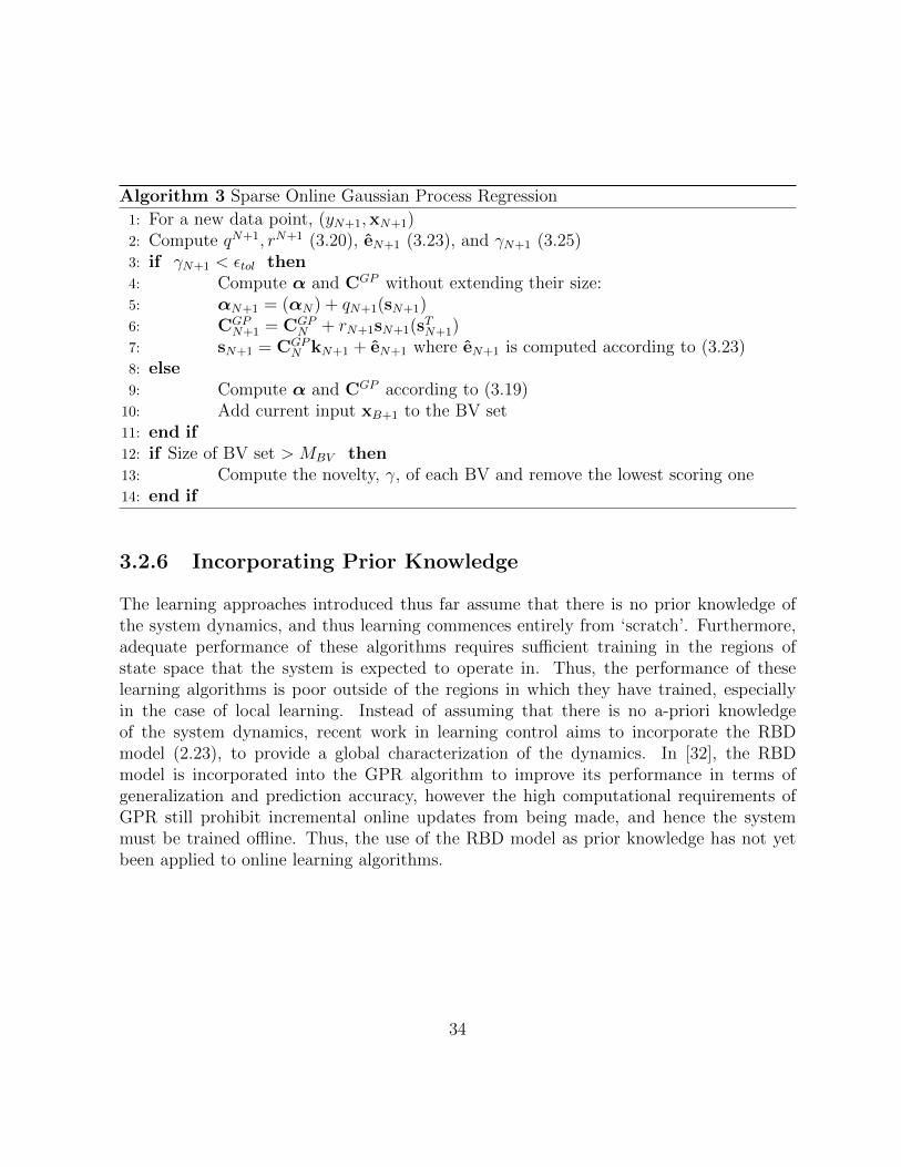
Algorithm 3 Sparse Online Gaussian Process Regression

1: For a new data point, (yN+1,xN+1)2: Compute qN+1, rN+1 (3.20), eN+1 (3.23), and γN+1 (3.25)3: if γN+1 < εtol then4: Compute α and CGP without extending their size:5: αN+1 = (αN) + qN+1(sN+1)6: CGP

N+1 = CGPN + rN+1sN+1(sTN+1)

7: sN+1 = CGPN kN+1 + eN+1 where eN+1 is computed according to (3.23)

8: else9: Compute α and CGP according to (3.19)

10: Add current input xB+1 to the BV set11: end if12: if Size of BV set > MBV then13: Compute the novelty, γ, of each BV and remove the lowest scoring one14: end if

3.2.6 Incorporating Prior Knowledge

The learning approaches introduced thus far assume that there is no prior knowledge ofthe system dynamics, and thus learning commences entirely from ‘scratch’. Furthermore,adequate performance of these algorithms requires sufficient training in the regions ofstate space that the system is expected to operate in. Thus, the performance of theselearning algorithms is poor outside of the regions in which they have trained, especiallyin the case of local learning. Instead of assuming that there is no a-priori knowledgeof the system dynamics, recent work in learning control aims to incorporate the RBDmodel (2.23), to provide a global characterization of the dynamics. In [32], the RBDmodel is incorporated into the GPR algorithm to improve its performance in terms ofgeneralization and prediction accuracy, however the high computational requirements ofGPR still prohibit incremental online updates from being made, and hence the systemmust be trained offline. Thus, the use of the RBD model as prior knowledge has not yetbeen applied to online learning algorithms.

34

Chapter 4

Comparison of Model-Based andLearning controllers

While much progress has been made in the field of adaptive control and the more recentlearning approaches to dealing with model uncertainty, little work has been carried outto compare the two. Burdet and Codourey [11] present a comparison between variouslearning approaches (such as Neural Networks and and ILC) and model-based adaptivecontrollers. Since then, there has not been any work in comparing the newer generationof regression-based learning (LWPR, SVM, GPR) techniques to the classical model-basedcontrol strategies. This chapter 1 focuses on evaluating Locally Weighted Projection Re-gression (LWPR) as an alternative to the model-based techniques such as computed torque(CT) or adaptive computed torque (ACT) control. Simulations are carried out in order toevaluate the position and orientation tracking performance of each controller while varyingtrajectory velocities, end-effector loading and errors in the known parameters.

In order to evaluate the performance of the LWPR learning controller, two model-basedcontrollers were also implemented: the computed torque (CT) controller in (2.41) and theadaptive computed torque (ACT) controller as described in Equation 3.2. The performanceof these controllers was evaluated in simulation using MATLAB/Simulink, the RoboticsToolbox (RTB) [13] and the open source LWPR code [55]. LWPR was used to learn thejoint space dynamics of a standard 6 DOF Puma 560 with the kinematic and dynamicparameters obtained from the RTB. The control loop executed at 1ms while the model wasupdated every 5ms for both the LWPR and ACT algorithms.

1A version of this chapter has been published. J. Sun de la Cruz, D. Kulic and W. Owen, A Compar-ison of Classical and Learning Controllers, World Congress of the International Federation of AutomaticControl, pp. 1102-1107, 2011.

35

4.1 Trajectories

In order to properly assess the performance of the model-based controllers, a trajectorywhich excites the dynamics of the system caused by inertia, gravity and Coriolis/centripetaleffects in (2.23) must be tracked. The figure-8 trajectory [31] is used, as it includes bothstraight and curved sections which induce significant torques from Coriolis/centripetal ef-fects. The figure-8 trajectory, as seen in Figure 4.1, is described by the following task spaceequations:

xd =w8

2sin(

2π

Kc

t) + xi

yd =l82

cos(4π

Kc

t) + yi −l82

zd = zi

(4.1)

where pd = [xd yd zd]T is the vector of the desired end-effector task space position, [xi yi zi]

is the desired Cartesian initial position, 2π/Kc is the desired duration of one cycle of thefigure-8 in seconds, and w8 and l8 are the width and length of the trajectory. The task-space trajectory in Equation 6.1 is converted to a joint space trajectory at a samplingrate of 1ms through the inverse kinematics algorithm in Chapter 2. Desired velocity andacceleration terms are generated through numerical differentiation also with a 1ms timestep using Matlab. All trajectory generation was carried out offline.

In addition to the figure-8 trajectory, a persistently exciting (PE) trajectory [14] is usedto provide sufficient excitation of the dynamics. This trajectory was designed directly inthe joint space as a linear combination of sinusoids given by:

qi = ai + bi

3∑l=1

(sin(wPEt) + cos(2wPEt)) (4.2)

where qi is the ith joint angle, ai and bi are constant scalars, and wPE is proportional tothe fundamental frequency. The resulting task space trajectory is a cardioid-like shape, asseen in Figure 4.6.

Simulation I

The first simulation compares the performance of the LWPR controller to the fixed param-eter computed torque controller at varying trajectory velocities. The figure-8 trajectory

36

in Equation (4.1) is tracked with parameters w8 = l8 = 0.2, [xi yi zi] = [−0.3, 0.1, 0]. Tovary the trajectory velocities, values of Kc = 1.57 and Kc = 2.09 were used, correspondingto frequencies of 0.25 and 0.3Hz. To evaluate orientation control, a sinusoidal signal wasinput as the desired orientation of the end-effector. The LWPR controller was trained for60s on the 0.25Hz trajectory, after which training was stopped and tracking performancewas evaluated. The system was then allowed to train for another 120s. Next the trajectoryfrequency was increased to 0.3Hz, and the system was trained for an additional 30s, afterwhich tracking performance was evaluated. These results are then compared against theCT controller. The durations of training were determined by observing the mean squarederror (MSE) of the predicted torques from the LWPR controller. Training was stoppedwhen asymptotic convergence of the MSE was observed. Since no parameter perturba-tion was introduced yet, only the CT and LWPR controllers are compared in the firstsimulation.

Simulation II

The second simulation evaluates tracking of the figure-8 pattern with varied end-effectorloads, thereby introducing model parameter errors. The trained system from the firstsimulation (0.25Hz and 180s training) was used to track the figure-8 trajectory, but withadditional end-effector masses of 0.5 and 1kg. The same conditions were repeated on theACT and CT controller. After 30s of training time for the LWPR controller and ACTcontroller, the performance of all three controllers was evaluated.

Simulation III

The third simulation adds varying amounts of error to the inertia parameters of the modelwhile observing the resulting performance of the three controllers when tracking the figure-8trajectory. Training of these models was done in the same manner as above.

Simulation IV

The fourth simulation introduces friction in addition to inertia parameter uncertainty whiletracking the persistently exciting (PE) trajectory in Equation (4.2) This trajectory is usedfor two reasons. Firstly, by using a trajectory with significant frequency content, the effectof persistence of excitation on the tracking and performance of ACT can be evaluated.Secondly, by shifting the operating range of the manipulator away from that of the figure 8

37

trajectory, the generalization performance of LWPR is tested. Furthermore, both Coulomband viscous friction are introduced into the simulation. In order to assess the ACT con-troller’s ability to cope with unmodeled dynamics, two cases are tested: one in which bothCoulomb and viscous friction (2.26) are modeled, and one in which only Coulomb frictionis modeled in the controller, but both types of friction are modeled in the plant. Thefriction constants were obtained from the defaults for the Puma 560 in the RTB.

4.2 Parameter Tuning and Initialization

Adaptive Computed Torque

The stability of the ACT controller was found to be highly sensitive to the adaptive gainparameter, γ (3.2). While a higher value of γ generally results in faster adaptation time,it increases the system’s sensitivity to noise and numerical errors from integration of thetime derivative of the estimated parameters (3.2). An adaptive gain of 0.01 was found tobe the best tradeoff.

LWPR

Although LWPR incorporates many algorithms which enable the system to automaticallyadjust its parameters for optimal performance, initial values of these parameters can sig-nificantly impact the convergence rate. The initial value for the distance parameter D(3.6) dictates how large a receptive field is upon initialization. Too small a value of D(corresponding to large receptive fields) tends to delay convergence while a larger value ofD results in overfitting of the data [55]. This parameter was generally tuned through atrial-and-error process which involved monitoring the MSE of the predicted values duringthe training phase. The initial performance of the LWPR controller is also highly depen-dent upon the data sets that are used to train the LWPR model. Because LWPR is a locallearning approach, it must be trained in the region(s) of input space that the manipulatorwill be operating in. In order to train the model, a low-gain PD controller was used totrack the desired trajectory while the LWPR model obtained training data. The initialvalue of the distance parameter D was set to 0.05 for each input dimension.

38

4.3 Results

Simulation I

The LWPR model was trained on the figure-8 trajectory at 0.25Hz, enabling it to predictthe necessary torques for tracking at frequencies near 0.25Hz. As seen in Figure 4.1 andTable 5.1, after an additional training period of 40s, the LWPR controller compensated forthe 0.3Hz trajectory, allowing it to perform nearly as well as the ideal CT controller. Thisillustrates the ability of the LWPR controller to rapidly adjust to changes in its operatingconditions. However, frequencies greater than 0.3Hz were sufficient to push the system farenough from the trained region of input space, eventually resulting in LWPR predicting ofzero for all the joint torques, causing the system to rely entirely on the feedback componentof the control law. This result highlights the sensitivity of the LWPR controller to the initialtraining set. A potential solution is a more complete initial training of the LWPR model. Ifthe initial training set were to include a larger subset of the input space obtained throughmotor babbling [39] for example, it is expected that the LWPR controller would be ableto handle larger perturbations.

−0.4 −0.35 −0.3 −0.25 −0.2

0

0.05

0.1

0.15

0.2

X [m]

Y [m

]

−1 0 1

x 10−3

0

0.05

0.1

0.15

0.2

Z [m]

RefCTLWPR InitialLWPR Final

Figure 4.1: Position Tracking at 0.25Hz

39

Frequency0.25Hz 0.3Hz

[mm] [deg] [mm] [deg]PD 4.07 0.89 5.54 2.89CT 1.80 0.15 2.03 0.22

LWPR Initial 3.56 1.67 4.68 2.54LWPR, 60s 2.71 1.31 / /LWPR, 180s 1.95 0.25 2.20 0.42

Table 4.1: Frequency - RMS position error [mm], orientation error [deg]

Simulation II

The second simulation evaluated the ability of the controllers to handle unmodeled end-effector loads. As seen in Table 5.2 and Figures 4.2 and 4.3, due to the unknown massof the end-effector, imperfect linearization and decoupling cause a decrease in trackingperformance of the CT controller. Both the LWPR and ACT controller are able to outper-form the CT controller after 30s of additional training. Although the ACT controller hasa-priori knowledge of the structure of the dynamic equation of the manipulator, it does notperform any better than the LWPR controller in position tracking after the same length ofadaptation time. This is due to the slow convergence of estimated masses to their actualvalues, which can in turn be explained by the relatively low adaptive gain and the lack ofa PE trajectory. However, as seen in the orientation results in Table 5.2, when trackingsinusoidal angular velocities on each joint of the wrist, the ACT controller yields better ori-entation tracking as compared to the LWPR controller, illustrating the importance of PEtrajectories in the performance of the ACT controller. The LWPR controller was able tolearn the inverse dynamics for both the 0.5kg and 1kg payload. However, masses greaterthan 1kg were sufficient to push the system to operate in a region outside its training,causing the controller to rely entirely on the feedback component of the control law. Inthis case, the performance of the LWPR controller was unable to converge due to the factthat the system was now operating so far from the desired trajectory that the receptivefields corresponding to the desired trajectory were never updated with new data.

Simulation III

Simulation three introduces parameter estimate errors into all the link masses, centreof mass locations and the moments of inertia of each link. Table 4.3 and Figures 4.4and 4.5 illustrate that inaccurate knowledge of the dynamic parameters causes significant

40

−0.4 −0.35 −0.3 −0.25 −0.20

0

0.05

0.1

0.15

0.2

X [m]

Y [m

]

RefCTLWPR 30sACT 30s

−5 0 5

x 10−3

0

0.05

0.1

0.15

0.2

Z [m]

Figure 4.2: Position Tracking with 0.5kg Load

Payload+0.5 kg +1kg

[mm] [deg] [mm] [deg]PD 7.34 0.92 19.07 3.39CT 4.95 0.60 16.45 2.15

ACT, 30s 4.44 0.44 2.70 1.26LWPR, +30s 4.16 0.65 7.01 1.29

Table 4.2: Payload - RMS position error [mm], orientation error [deg]

degradation in performance for the CT controller, due to the imperfect linearization ofthe system dynamics. As seen in Table 4.3, the performance of the ACT controller wasparticularly poor in comparison to the LWPR controller, and even the CT controller. Thiscan be explained by the fact that the perturbation of the inertia parameters was appliedto all the joints of the manipulator, unlike the case of end-effector loading where only theparameters of one link were perturbed. Hence, it is expected that the adaptive controllerwould require both a persistently exciting trajectory, which excites all the dynamic modes ofthe structure, [14] and a longer adaptation time than 30s to yield better tracking results inthis scenario. The importance of PE trajectories will be illustrated in the next simulation.For the LWPR controller, similar findings to that of simulations one and two were observedin that inertia parameter perturbations greater than 10% were sufficient to prevent LWPRfrom predicting accurate joint torques, causing the system to rely entirely on the feedbackportion of the control law.

41

−0.4 −0.35 −0.3 −0.25 −0.2

0

0.05

0.1

0.15

0.2

X [m]

Y [m

]

RefCTLWPR 30sACT 30s

−10 −5 0 5

x 10−3

0

0.05

0.1

0.15

0.2

Z [m]

Figure 4.3: Position Tracking with 1kg Load

Parameter Error+1% +5%

[mm] [deg] [mm] [deg]PD 4.56 1.32 4.56 1.32CT 2.15 0.25 2.65 0.30

ACT, 40s 2.20 0.12 2.75 0.15LWPR, +40s 1.55 0.75 1.66 0.86

Table 4.3: Parameter Error - RMS position error [mm], orientation error [deg]

Simulation IV

Simulation four introduces the PE trajectory and Coulomb and viscous friction in addi-tion to inertia parameter error. As seen in Table 4.3, the CT controller performed thepoorest due to the error in its model parameters. When the ACT is implemented with thefull friction model, the resulting tracking performance is significantly better than the CTcontroller, as also shown in Table 4.3.

However, when only partial knowledge of the model is available (in this case only viscousfriction), the performance gain is no longer observed. The ACT controller outperforms theLWPR controller only if the friction model is fully known. This illustrates the importanceof: 1) a persistently exciting trajectory and 2) accurate knowledge of structure of thedynamic model when using adaptive control.

The PE trajectory was also chosen to be significantly different from the figure 8 in order

42

−0.4 −0.35 −0.3 −0.25 −0.2

0

0.05

0.1

0.15

0.2

X [m]

Y [m

]

RefCTLWPR 30sACT 30s

−2 0 2

x 10−3

0

0.05

0.1

0.15

0.2

Z [m]

Figure 4.4: Position Tracking with 1% Parameter Error

to test the generalization of the LWPR model. The first test involved using the model thatwas learned in simulation three to attempt to track the PE trajectory. This model hadseen roughly 10,000 training points, all of which were localized to the figure 8 trajectory.As expected, this LWPR model was unable to predict torques in the operating range ofthe PE trajectory. Hence, the LWPR model had to be re-trained on the PE trajectory,taking roughly 240 seconds to achieve good performance in the presence of friction.This simulation was then repeated with a model that was initialized through the use ofmotor babbling [39]. Here, a joint space trajectory was made by randomly selecting apoint in the robot’s expected operating range about which small sinusoidal trajectorieswere executed by the joints. This sequence was repeated at different points until sufficientcoverage of the operating range was seen. Roughly 10,000 training points were generatedfrom motor babbling. A PD controller was then used to track this trajectory and theresulting data was used to train the LWPR model. As seen in Table 4.3, by initializing theLWPR model this way, good performance on the PE trajectory could be learned in halfthe time compared to the case without motor babbling.

Even without any a-priori knowledge of the structure or parameters of the dynamics,LWPR is able to learn the inverse dynamics function of a manipulator accurately enough toyield near-optimal control results within minutes of training. Unlike the adaptive controllerwhich relies on persistence of excitation for tracking performance, the LWPR approach canbe trained on an arbitrary trajectory provided that it is given sufficient time to learn.

When tracking a PE trajectory with a known dynamic model, the ACT clearly outper-forms the LWPR controller in terms of tracking accuracy and adaptation time, which is

43

−0.4 −0.35 −0.3 −0.25 −0.2

0

0.05

0.1

0.15

0.2

X [m]

Y [m

]

RefCTLWPR 30sACT 30s

−2 −1 0 1

x 10−3

0

0.05

0.1

0.15

0.2

Z [m]

Figure 4.5: Position Tracking with 5% Parameter Error

Parameter Error+1% +5%

[mm] [deg] [mm] [deg]PD 4.12 0.95 4.12 0.95CT 2.45 0.55 3.10 0.80

ACT, partial friction, 40s 2.0 0.40 2.1 0.45ACT, full friction, 40s 1.65 0.30 1.70 0.32

LWPR, 240s 1.75 0.45 1.80 0.50LWPR, motor babbling, 120s 1.82 0.50 1.85 0.55

Table 4.4: Parameter Error and Friction - RMS position error [mm], orientation error [deg]

expected due to its incorporation of a-priori knowledge. However, if LWPR is presentedwith sufficient time to learn, its performance will closely approach that of ACT, but will notsurpass it due to the use of local linear approximations of the system dynamics. However,the ACT controller is at a disadvantage since not all trajectories meet the PE requirement.For this reason, the identification of system parameters is often done offline on a prede-termined trajectory which is optimized to yield the best parameter estimates [24]. Whilethis may yield results better than the LWPR controller, the benefits of online, incrementallearning are lost, where LWPR excels.

The performance of LWPR outside of areas in which it has trained is poor. Thiswas clearly illustrated when a large perturbation to the inertia parameters caused themanipulator to move outside its trained region, rendering the system completely reliant

44

−0.3 −0.2 −0.1 0 0.1 0.2 0.3−0.2

−0.1

0

0.1

0.2

0.3

0.4

0.5

X [m]

Y [m

]

0 0.1 0.2 0.3 0.4−0.2

−0.1

0

0.1

0.2

0.3

0.4

0.5

Z[m]

RefCTLWPRACT

Figure 4.6: PE Trajectory - 5% inertia and friction error

upon the feedback portion of the control law. This problem can be overcome throughproper initialization of the model through motor babbling. However, for applications inwhich the manipulator workspace is large, significant amounts of training covering therobot’s entire workspace must be carried out in order to achieve good results. This is notan issue for the adaptive controller, as it incorporates a-priori knowledge of the systemdynamics, which is applicable to the entire workspace of the robot.

4.4 Summary

These simulations indicate that the performance of the CT control scheme is highly de-pendent upon accurate knowledge of the dynamic parameters of the system. A slightperturbation from the actual inertia and friction parameters of the system caused a de-crease in performance, while the LWPR and ACT performance remained more consistentunder the same conditions.

The ACT approach was able to outperform the CT controller in most scenarios due toits ability to generate online estimates of the actual inertia parameters of the system. It wasshown that when the trajectory is persistently exciting and the structure of the dynamics is

45

well known, the ACT controller also outperforms the LWPR. However, in practice, not alltrajectories are PE and the structure of the friction model may not be known well. Hence,it is expected that when dealing with a physical robot, the simplified models of frictionused in this paper will further degrade the performance of the ACT controller while theLWPR will be able to learn the additional nonlinearities present in the physical robot.

Lastly, although the LWPR controller was able to handle parametric uncertainty with-out any a-priori knowledge of the system, its greatest limitation is its local learning, whichdictates that successful performance requires adequate initial training of the system. Sig-nificant perturbations caused the system to operate outside of its trained region, resultingin the system relying solely on the feedback component of the control law for trackingperformance. Initializing the model through motor babbling can partially mitigate thisissue, but the larger the workspace of the robot, the larger the training data set must be.

46

Chapter 5

Incorporating Prior Knowledge

In the previous chapter, the ability of learning controllers to cope with varying levels andsources of parametric uncertainty was illustrated. However, this performance is contingentupon the availability of large amounts of relevant training data for the algorithm, especiallyfor the case of local learning techniques such as LWPR. This chapter 1 presents two types ofonline, incremental learning algorithms which incorporate prior knowledge to improve thegeneralization performance of the machine learning algorithms. An approach is developedfor incorporating prior knowledge for both local (LWPR) and global (GPR) learning. Priorknowledge is incorporated into the LWPR framework by initializing the local linear modelswith a first order approximation of the available prior information. Prior knowledge isincorporated into the mean function of Sparse Pseudo Input Gaussian Processes (SPGP)and Sparse Online Gaussian Process (SOGP) regression, and a modified version of thealgorithms is proposed to allow for online, incremental updates. It is shown that theproposed approaches allow the system to operate well even without any initial trainingdata, and further improve performance with additional online training.

5.1 Prior Knowledge

The RBD equation (2.23) provides a globally valid model representing the dynamics of arobot manipulator. Hence, providing the RBD equation as prior knowledge to the learning

1A version of this chapter has been published. J. Sun de la Cruz, D. Kulic and W. Owen, OnlineIncremental Learning of Inverse Dynamics Incorporating Prior Knowledge, International Conference ofAutonomous and Intelligent Systems, pp. 167-176, 2011.

47

controllers would greatly improve their generalization performance. However, due to thecomplexity of robotic systems, obtaining a complete and accurate RBD model can bedifficult and tedious. Therefore, even if partial knowledge of the RBD model is available,this information should be incorporated into the learning algorithms to potentially boostperformance. The simplest term of the RBD model in (2.23) is the gravity loading vector,G(q) (2.22), as it depends upon the least number of inertial parameters of the systemcompared to the inertia and centripetal/Coriolis terms of the model [45]. In this chapter,techniques for incorporating partial prior knowledge to reduce training requirements forlearning controllers are developed.

5.2 LWPR

Although LWPR has the ability to learn in an online, incremental manner due to its locallearning approach, performance deteriorates quickly as the system moves outside of theregion of state space it has been trained in, as demonstrated in Chapter 4. In order toimprove the generalization performance of LWPR, an algorithm for incorporating a-prioriknowledge from the RBD model (2.23) into the LWPR algorithm is proposed. This is doneby initializing the receptive fields in the LWPR model with a first order approximation ofthe available RBD model:

β ← ∂τ

∂xx=x∗ (5.1)

where x∗ is a new query point for which no previous training data has been observed andτ(x∗) is the known or partially known dynamics. Equation 5.1 represents the linearizationof the known system dynamics about a particular state of the system known as the querypoint, x∗. Although expressions for this linearization can be derived analytically, dueto the complexity of the system dynamics, linearization is performed through numericalperturbation about the query point x∗:

βik =τi(x

∗k−tol)− τi(x∗)

tol(5.2)

where βik is the slope of the linearized model relating the ith output dimension to the kth

input dimension, x∗k−tol is the perturbed query point where tol is subtracted from the kth

element of the query vector x∗, and tol is the perturbation tolerance, which is set to asmall value for accuracy, i.e. tol = 10−5.

For a query point x∗ and the known RBD equation τ (x), the algorithm shown inAlgorithm 4 for initializing the LWPR model is added to the standard prediction procedure

48

of LWPR:

Algorithm 4 LWPR with Prior Knowledge

1: if there is no existing RF centered near x∗ then2: Compute (β) according to (5.1)3: Initialize a new RF centered at x∗ with hyperparameters β4: else5: Compute prediction with standard LWPR procedure (3.2.1)6: end if

The determination of whether an existing RF is centered near x∗ is made in the sameway as determining whether a new RF should be added, as described in Section 3.2.1, i.e.,if there is no existing RF that produces a weight (3.6) greater than wgen given x∗, theinitialization procedure is applied.

By evaluating the partial derivative of the RBD equation (2.23) at the query point, afirst-order linear approximation of the system dynamics is obtained, and is used to initializethe model at that point. The size of the receptive field is initially set as a tunable parameter,and is eventually learned optimally through gradient descent as outlined in Chapter 3.

5.3 GPR Approaches

With Gaussian process regression techniques, including the SPGP and SOGP algorithmsdescribed in Sections 3.2.4 and 3.2.5, typically a zero mean function for the Gaussianprocess is assumed, and hence predictions in areas of the workspace where few trainingpoints have been observed are inaccurate. A simple method of incorporating a-prioriknowledge is to set the mean function in Equation (3.10) equal to the available model ofthe system, thus biasing the system towards the specified a-priori knowledge [32].

While the mean function is biased towards the prior knowledge, the covariance functionk (3.10) still requires adaptation to the data that is observed. Specifically, the hyperpa-rameters of the covariance function, as described in Section 3.2.3 must be optimized tothe incoming training data. Nonlinear conjugate gradient descent (NCG) [46] is used tominimize the negative log marginal likelihood with respect to the hyperparameters, Θ.As an iterative gradient-based optimization technique, NCG requires the specification ofan initial guess of Θ, which is determined by performing the optimization on a batch oftraining data collected from the system during motor babbling in Chapter 4.

49

With standard gradient descent optimization, the location, χ, of the extremum of afunction, f , is found by iteratively taking steps in the direction of the gradient of thefunction at the current point. That is:

χi+1 = χi + aidi (5.3)

where χi is the current solution (ith iteration) to the optimization problem, ai representsthe length of the step to be taken, and di is the step direction. This iterative procedureoften results in steps being taken in the same direction as in earlier steps resulting in aslower convergence. By employing NCG, this repetition is avoided by ensuring that allsearch directions are conjugate, or A-orthogonal, and that the necessary step lengths aretaken such that only one step must be taken in each search direction to arrive at theextremum for that direction. Thus, the convergence of NCG is better than or at leastthe same as standard gradient descent. A comparison between the convergence of NCGand standard gradient descent is illustrated in Figure 5.1, where a 2-dimensional exampleis given, where the green lines represent gradient descent convergence and the red linesrepresent NCG.

Figure 5.1: Convergence of Gradient Descent vs NCG

Two vectors, di and dj, are conjugate, or A-orthogonal, if they have the followingproperty:

dTi Adj = 0 (5.4)

where A is a positive semi-definite matrix. In order to find the set of conjugate search

50

directions, d, the Polak-Ribiere formula is used to generate coefficients ξ:

ξi+1 =rTi+1(ri+1 − ri)

rTi ri(5.5)

where i represents the current iteration, and the residual r is set to the negation of thegradient at the current location χi, i.e. r = −f ′(χi). Thus, the conjugate search directions,d, can be determined:

di+1 = ri+1 + ξi+1di (5.6)

With the selection of the step direction, di, the problem is reduced to a one-dimensionaloptimization case which involves finding the best step length, a, to take in direction di. Thisis done by through the use of a line search procedure which finds the ai that minimizes f(χi+aidi). The interpolation method of line searching achieves this by firstly approximatingthe function f(χ + ad) as a polynomial through a Taylor series expansion. Here we dropthe iteration index for simplicity:

f(χ+ ad) ≈f(χ) + a[d

daf(χ+ ad)]a=0 +

a2

2[d2

da2f(χ+ ad)]a=0

=f(χ) + a[f ′(χ)]Td +a2

2dT f ′′(χ)d

(5.7)

The secant method is then used to approximate the second derivative, f ′′, as a finitedifference equation of the first derivative f ′ evaluated at two points, a = 0 and a = σ:

d2

da2≈ 1

σ[f ′(χ+ σd)]Td− [f ′(χ)]Td (5.8)

where σ is a non-zero number such that the closer σ is to 0, the better the approximationof the second derivative. Substituting this expression into (5.7) and differentiating:

d

daf(χ+ ad) ≈ [f ′(χ)]Td +

a

σ

[f ′(χ+ σd)]Td− [f ′(χ)]Td

(5.9)

Minimization of f(χ + ad) can then be achieved by equating its derivative to zero andrearranging for a:

a = −σ ζ

ζprev − ζ(5.10)

where ζprev = [f ′(χ+ σd)]Td and ζ = [f ′(χ)]Td. This process is then repeated, with thecurrent χ equated to the value of χ + ad calculated in the previous iteration. The stop

51

condition for the line search is based on the gradient approaching orthogonality with thecurrent search direction, i.e. f ′ Td ≈ 0. High tolerances for this term have been foundto be too computationally inefficient for the relatively small gain in accuracy [46] that isachieved.

Algorithm 5 Nonlinear Conjugate Gradient Optimization

1: given: initial guess χ, maximum allowable CG and line search iterations, εCG, εLS2: initialize: r← −f ′(χ), d← r, i← 03: while i < imax and ‖ri‖ ≤ εCG‖r0‖ do4: initialize: j ← 05: ζprev ← [f ′(χ+ σd)]Td6: do7: ζ ← [f ′(χ)]Td8: a← −σ ζ

ζprev−ζ9: χ← χ+ adi

10: ζprev ← ζ11: j ← j + 112: while j < jmax and ‖ad‖ ≤ εLS13: rprev ← r14: r← −f ′(χ)

15: ξ ← rT (r−rprev)

rTprevrprev

16: d← r + ξd17: i← i+ 118: end while

In order to test the effects of limiting the maximum number of line search iterationson the accuracy of the SPGP algorithm, the system was trained on data sets obtainedfrom the simulations in Chapter 4 and the MSE of prediction was monitored. In thefirst case, illustrated at the top of Figure 5.2, up to 50 line search iterations were allowed(i.e. jmax = 50), and below in the second graph, 25 iterations were allowed. Despite thisdifference, the final MSE of both cases is nearly identical. The only noticeable discrepancyis the initially slower rate of convergence of the joints in the case of early line searchtermination. Joint 1 also exhibits non-monotonic convergence initially. However, due tothe lower number of allowable line search iterations, the computational burden is reducedand thus the frequency at which the overall hyperparameter updates are performed can beincreased. Hence, for the simulations, less accurate, but more frequent line searches wereused by terminating the search after 25 iterations.

52

0 1000 2000 3000 4000 5000 60000

10

20

30

40

50

Pre

dict

ion

MS

E

Maximum 50 Line Search Iterations

Joint 1Joint 2Joint 3

0 1000 2000 3000 4000 5000 60000

10

20

30

40

50

Sample [Ts = 0.001s]

Pre

dict

ion

MS

E

Maximum 25 Line Search Iterations

Figure 5.2: Prediction MSE

Despite its improved convergence over standard gradient descent, each call to NCGoptimization requires a significant number of time steps of the control loop to compute.Thus, the code is broken down into a sequence of smaller, ‘atomic’ code segments, so thatthe computation of NCG occurs over multiple controller time steps. This was done sothat each code segment would have at most one call to evaluate the function derivative f ′.Based on Algorithm 5, the code segments are separated into lines 1 : 2, 3 : 5, 6 : 12 and13 : 18, with each code segment being executed over a single time step of the controller.The optimized location of the hyperparameters, represented by χ, is not used in the controlloop until the entire algorithm has been executed.

5.3.1 Simulation Setup

The proposed approaches are evaluated in simulation on a 6-DOF Puma 560 robot usingthe Robotics Toolbox (RTB) [13]. The open-source LWPR [55], SPGP [50] and SOGP[16] code were modified to incorporate a-priori knowledge and incremental updating asdescribed above. In order to simulate the nonlinearities present in a physical robot, theeffects of Coloumb and viscous friction were simulated according to Equation 2.26, with thefriction constants obtained from the defaults for the Puma 560 in the RTB. Furthermore,to simulate the effects of imprecise knowledge of the inertial parameters of the robot, a10% percent error in the inertial parameters of the a-priori knowledge was introduced. ForLWPR, the tunable parameters were set to the same values as determined in Chapter 4.

53

For SPGP and SOGP, the maximum size of the sparse subset of datapoints, M , was setto 35. This number was determined by trial-and-error to be the smallest possible valuebefore a noticeable degradation in prediction performance was introduced.

A-priori knowledge from the full RBD model in (2.23), or partial knowledge from thegravity loading vector (2.22) are used to initialize each algorithm. Standard computedtorque control (2.41) is also implemented for comparison.

Tracking performance of the controllers is evaluated on a ‘star-like’ asterisk pattern [31].The asterisk trajectory is a more challenging trajectory than the figure-8 due to the highcomponents of velocity and acceleration, and thus requires model-based control for goodtracking accuracy. Illustrated in Figure 5.3, this trajectory is formed in the horizontal XYplane, by first moving in a straight line outwards from a centre point, then retracing backinwards to the centre, repeating this pattern in eight different directions in a sequentialmanner. The inverse kinematics algorithm presented in Chapter 2 is used to convert thistrajectory from task to joint space.

0 0.05 0.1 0.15 0.2

−0.5

−0.45

−0.4

−0.35

−0.3

X [m]

Y [m

]

Figure 5.3: ‘Asterisk’ trajectory

54

1 2 3 4 5 6 7 8 9 100.8

0.9

1

1.1

1.2

1.3

1.4

1.5

Time [s]

Join

t Ang

le [r

ad]

RefCTLWPR RBD InitSPGP RBD InitSOGP RBD InitLWPR No PriorSPGP No PriorSOGP No Prior

Figure 5.4: Initial Tracking Performance for Joint 2 with full RBD Prior and No Prior

5.3.2 Results

Full Knowledge of RBD

Figure 5.4 depicts the joint space tracking performance of the computed torque (CT)controller using a model with 10% error in the inertial and friction parameters of thesystem. As seen from the figure, the parameter error causes poor tracking results. The sameRBD model is used to initialize both GP and LWPR models, and the resulting controllersare trained online while tracking the asterisk trajectory. Figure 5.4 and Table 5.1 showthe joint space tracking performance after one cycle of the trajectory. The performanceof the GP controllers is very similar to that of the computed torque controller, as theyare initialized with the same RBD equation. On the other hand, as the LWPR model isinitialized with a set of linear approximations of RBD equation, the initial performance ofLWPR is not as good as the GP or the CT methods.

Figure 5.5 and Table 5.1 show the results after 90 seconds of additional training. Dueto the high computational efficiency of LWPR, incremental updates are made at a rate of400 Hz, while the more computationally taxing GP algorithms limit updates to a rate of100 Hz. Hence, as time progresses, LWPR is able to accumulate more training data thanthe GP controllers, eventually performing nearly as well as SPGP and SOGP. Initially,SPGP performs better than SOGP due to the fact that SPGP uses the full M = 35 sparseinputs from the start, whereas SOGP is initialized with M = 1 and adds sparse inputsas data is incrementally processed until the limit M = 35 is reached. Thus, after seeing

55

1 2 3 4 5 6 7 8 9 100.95

1

1.05

1.1

1.15

1.2

1.25

Time [s]

Join

t Ang

le [r

ad]

RefCTLWPR RBD FinalSPGP RBD FinalSOGP RBD Final

Figure 5.5: Final Tracking Performance for Joints 2 with full RBD Prior

significant amounts of training data, both SOGP and SPGP perform very similarly. Lastly,given sufficient data, all three learning controllers are able to outperform the CT methodby learning the nonlinear behaviour of Coloumb and viscous friction and compensating forthe initial inaccurate knowledge of the RBD equation.

Joint 1 2 3 4 5 6 AvgLWPR, Initial 1.25 2.26 1.74 0.65 0.75 0.80 1.24

LWPR, 90s 0.75 0.94 0.82 0.25 0.38 0.45 0.60SPGP, Initial 1.10 1.75 1.55 0.60 0.68 0.75 1.07

SPGP, 90s 0.70 0.85 0.78 0.22 0.32 0.45 0.55SOGP, Initial 1.21 1.88 1.60 0.63 0.70 0.82 1.14

SOGP, 90s 0.72 0.84 0.80 0.22 0.32 0.47 0.56

Table 5.1: RMS tracking error with full knowledge (deg)

Partial Knowledge of RBD

Figure 5.6 and Table 5.2 illustrate the joint space tracking performance of the SPGP,SOGP and LWPR models when initialized with only the gravity loading vector (2.22) ofthe RBD equation. In this case, LWPR outperforms SPGP during the first cycle. Thiscan be attributed to the higher update rate of LWPR, allowing the model to adapt more

56

quickly to the data it receives. After multiple cycles through the trajectory, this advantageof LWPR vanishes, as the GP models have then observed enough training data across theentire asterisk trajectory to learn a more accurate model. Figure 5.7 and Table 5.2 illustratethe performance after 150 seconds of training. Similarly to the case of full knowledge ofthe RBD, the learning controllers have all compensated for friction and clearly outperformthe CT controller. However, since the system was initialized with only partial knowledgeof the RBD equation, it has taken longer for both models to achieve the same trackingperformance in the case of full RBD knowledge. Similarly to the case of full knowledge ofRBD, SPGP initially performs better than SOGP, but after training this discrepancy isminimized.

0 1 2 3 4 5 6 7 8 9 100.8

0.9

1

1.1

1.2

1.3

1.4

1.5

1.6

Time [s]

Join

t Ang

le [r

ad]

RefCTLWPR Grav InitSPGP Grav InitSOGP Grav InitLWPR No PriorSPGP No PriorSOGP No Prior

Figure 5.6: Initial Tracking Performance for Joint 2 with Gravity Prior and No Prior

Joint 1 2 3 4 5 6 AvgLWPR, Initial 2.57 4.78 3.62 0.95 0.80 0.75 2.25LWPR, 150s 0.80 0.95 0.80 0.22 0.41 0.44 0.60SPGP, Initial 0.48 6.66 5.29 0.05 0.12 0.27 2.15SPGP, 150s 0.75 0.84 0.75 0.25 0.30 0.40 0.55

SOGP, Initial 0.50 6.75 5.43 0.10 0.14 0.30 2.20SOGP, 150s 0.77 0.83 0.76 0.25 0.32 0.39 0.55

Table 5.2: RMS tracking error with partial knowledge (deg)

Without the use of a-priori knowledge, learning algorithms were typically initializedwith large training data sets obtained through motor babbling [55], [39], [33] in order to

57

0 1 2 3 4 5 6 7 8 9 100.95

1

1.05

1.1

1.15

1.2

1.25

1.3

Time [s]

Join

t Ang

le [r

ad]

RefCTLWPR Grav FinalSPGP Grav FinalSOGP Grav Final

Figure 5.7: Final Tracking Performance for Joints 2 with Gravity Prior

achieve decent tracking performance after initialization. By incorporating a-priori knowl-edge of the RBD equation, whether partial or full, it is shown in these results that theproposed systems are able to perform reasonably well from the start, even without under-going such an initialization procedure.

Algorithm Computation Time

In order to evaluate the computational efficiency of LWPR, SPGP and SOGP, each al-gorithm was trained on data sets of varying size (2,4,6,8,10,12 and 14 thousand trainingpoints) obtained from the simulation work in this chapter. Figure 5.8 illustrates the compu-tation time required to compute a single torque prediction given an input x∗ as a functionof the number of training data points that the algorithm has processed. The results wereobtained on a PC running Windows XP with a CPU clock speed of 2.66 GHz and 4 GBof RAM. For SOGP and SPGP, the maximum size of the sparse representation set waslimited to 35.

As seen in Figure 5.8, LWPR has the lowest computational cost which remains relativelyconstant with an increasing data set size. This is due to the fact that LWPR does notexplicitly store the entire training set, but rather incorporates them into local linear models.For the sparse GP techniques, SOGP clearly outperforms SPGP. This can be attributedto the online procedure of SOGP which allows data points to be processed incrementally.Although SPGP also uses a sparse representation, data is still processed in batches, and

58

no provision for incremental updates is provided. Because of this, the computation timefor a single prediction from SPGP increases much more rapidly than SOGP as the numberof training points increases.

Although the simulation results presented in this chapter show that the SPGP controllermarginally outperforms the SOGP controller in terms of tracking performance (see Tables5.1 and 5.2), the performance gains from SPGP are not significant enough to offset thehigher computational costs which increase significantly as the training data set increases.Although the simulation platform was able to handle the computational requirements forSPGP while maintaining near-real time performance, it should be noted that this wasonly for 150 seconds of operation (corresponding to 15,000 training points). For long-termincremental learning, it is expected that the computational requirements of SPGP willprohibit real-time control. Thus, for the following chapters, SOGP is chosen over SPGP.

2000 4000 6000 8000 10000 12000 140000

2

4

6

8

10

12

14

16

Number of training points

Com

puta

tion

time

[ms]

LWPRSOGPSPGP

Figure 5.8: Computation time required for a single prediction

59

Chapter 6

Experimental Work

The results presented in Chapters 4 and 5 are all carried out in simulation using MAT-LAB/Simulink. In order to closely simulate the nonlinear dynamics present in a physicalsystem, the effects of Coulomb and viscous friction were introduced in simulation. In thischapter, the results of experimental work on a physical robot, in addition to simulations, arereported to fully evaluate the performance of the proposed methods. Experimental workwas conducted at the Collaborative Advanced Robotics and Intelligent Systems (CARIS)Laboratory at the University of British Columbia.

6.1 Experimental Platform

All experimental work was carried out on a CRS A460 robotic manipulator with a customdesigned open-architecture controller [21] developed and fabricated in the UBC CARISlab. Use of the CARIS open-architecture controller was necessary to bypass the defaultfactory PID control architecture, allowing voltage commands to be issued to the DC servomotors actuating the arm. The open-architecture controller is illustrated in Figure 6.1and consists of a custom motor amplifier unit and a PC with a processor speed of 2.4GHzand 2 GB of RAM running Windows XP. The Ardence RTX real-time kernel [1] is usedto allow RTX processes to take priority over Windows processes during CPU scheduling,thus allowing real-time performance of the control system. Quanser’s Wincon software [2]allows Simulink-coded controllers to be compiled into C code which can then be executedon a Wincon client running as an RTX kernel process. The controller sampling time is setto 1 ms, which is the lowest setting achievable by the Wincon system.

60

Figure 6.1: CRS Open-Control Architecture, adapted from [2]

Due to the requirements of the Wincon system, the algorithms written in C/C++ code(LWPR, SOGP, and RNE) were wrapped in C-coded S-functions and called as Simulinkfunction blocks. The multi-rate block sampling function of the Simulink engine allowedthe computationally-expensive functions to be executed at a slower sampling rate. For theLWPR experiments, updates to the learned model are processed at a frequency of 100 Hz,or at every 10th sample of the global 1ms sample time. These were the maximum updaterates and settings achievable by the controller hardware. Due to the limited availabilityof the CRS arm at the CARIS lab, experimental work for the SOGP controller couldnot be completed, and simulation results (indicated by SIM ) are presented for the SOGPcontroller instead. For these simulations, the same global time step of 1ms was used, theupdates are processed at a frequency of 10 Hz, and hyperparameter updates are completedat a rate of 1 Hz. The number of basis vectors for SOGP was set to 35.

6.2 Dynamic Parameters

The dynamic parameters for the CRS arm (link mass, location of centre of mass and inertiamatrix values) were obtained from the results presented in [40] which were determinedoffline through the procedure of dynamic parameter identification as described briefly inChapter 3. The identified parameters were manually checked and corrected to ensure thatthey made physical sense. For example, the location of the centre of mass location for link2 was identified in [40] as being outside the volume of the link itself. Thus, the identifiedvalue was replaced with the approximate location of the volumetric centroid of the link,as physically measured by the author. These parameters were then used to calculatethe RBD model (2.23) and the gravity vector (2.22) for initialization of LWPR. The motor

61

parameters (rotor inertia, damping and torque constant) for the joint motors were obtaineddirectly from the manufacturer specification sheet.

For the SOGP simulations, the CRS A460 arm was modeled using the kinematic pa-rameters supplied in the user’s manual. The same dynamic parameters obtained above forthe LWPR experiments are used for the SOGP controller. For the plant model used in theSOGP simulations, the available dynamic parameters of the CRS arm were perturbed untilthe performance of the experimentally implemented FF controller matched that of the sim-ulated FF controller as closely as possible. This was done so that the results in simulationwould be comparable to the experimental results obtained for the LWPR controller.

6.3 Experiments

The following test cases were carried out for the Feedforward (FF), LWPR, and SOGPcontrollers in order to evaluate their ability to deal with uncertainty in the dynamic model:

1. Tracking a figure-8 trajectory by initializing the system through Motor Babbling(MB), rigid body dynamics (RBD) and gravity loading information

2. Tracking a figure-8 trajectory at different frequencies and varied end-effector masses

The FF and LWPR controllers were tested experimentally on the CRS A460 arm whilethe tests for the SOGP controller were carried out in simulation as described above. Asseen in Figure 6.2, a figure-8 trajectory in the horizontal XY plane, covering a length andwidth of approximately 0.2m x 0.4m, is used to test the trajectory-following capabilities ofthe controllers. Due to the limited processing power of the control PC for the CRS arm,only the first three degrees of freedom of the manipulator were used - corresponding toposition-only control.

The task space equations for ‘the figure 8’ trajectory are as follows:

xd = 0.1 sin(2π

Tct)− 0.47

yd = 0.2 cos(4π

Tct)

zd = 0.29

(6.1)

where pd = [xd yd zd]T is the vector of the desired end-effector task space position, and

Tc is the desired duration of one cycle of the figure-8 in seconds. Desired velocity andacceleration terms are generated through numerical differentiation as in Chapter 4.

62

Figure 6.2: Figure-8 trajectory

The simulation work carried out in Chapter 4 assumed that the commands to jointactuators were issued directly as torques. However, with the open-architecture controller,motor commands are issued in voltages and not torques. Thus, the LWPR and simu-lated SOGP controllers were used to learn both the dynamics of the arm (2.23) as wellas the motor dynamics (2.27). The mapping to be learned by LWPR and SOGP is given by:

(q, q, qd) 7→ vm (6.2)

where vm is the vector of motor voltages for each joint.

6.3.1 Feedforward vs Computed Torque

Both the feedforward (FF) and Computed Torque (CT) controllers presented in Chapter2 were implemented experimentally to determine which control strategy is the most effec-tive. For the FF controller, desired joint velocities and accelerations were computed offlinethrough numerical differentiation of the desired joint angles. For the CT controller, some

63

form of state estimation [37], [57] was required to determine the joint velocity and acceler-ation signals given the joint angles as measured by the encoders. Numerical differentiationwas also used for the CT controller. However, due to the quantization of the joint encoders,significant amounts of noise were introduced into the differentiated signals. To solve this,a second-order Butterworth filter was used to smooth out the noise caused by numericaldifferentiation. The filter was designed using the Filter design toolbox in MATLAB andwas implemented at 1KHz, which is the smallest allowable sampling time in Wincon. Boththe FF and CT controller were used to track the figure-8 trajectory in Equation 6.1. Asseen in Figure 6.3 and Table 6.1, the FF controller is able to outperform the CT controller.Part of the reason for this discrepancy in performance is likely due to the use of the But-terworth filter at 1KHz, which injects a significant delay into the resulting filtered signalsof the desired velocity and acceleration. If the experimental system was able to operateat a higher frequency, or if sufficient computational resources were available to implementa non-linear observer [37], the CT controller may have been able to outperform the FFcontroller, as the cancelation of the nonlinear dynamics would be more accurate about theactual, rather than the desired trajectory.

0.45 0.5 0.55 0.6 0.65−0.25

−0.2

−0.15

−0.1

−0.05

0

0.05

0.1

0.15

0.2

0.25

X [m]

Y [m

]

RefCTFF

Figure 6.3: FF vs CT Tracking Performance

64

Joint 1 2 3 Avg

FF 1.75 0.88 1.51 1.38CT 1.82 1.05 1.78 1.55

Table 6.1: FF vs CT RMS Joint Space Error (deg)

6.3.2 Initialization Technique

The effects of different initialization strategies on LWPR tracking performance are shownin Figure 6.6. For this experiment, LWPR was initialized either through motor babbling,or through full or partial knowledge of the RBD equation as outlined in Chapter 5. Thesame motor babbling strategy as in Chapter 4 was applied for this experiment, resultingin roughly 50,000 initial training points from motor babbling. For LWPR, the full 50,000training points were used for initialization. Initially, the performance of LWPR with motorbabbling initialization is consistently better than both RBD and gravity vector initializa-tion for all three joints. This is due to the inaccuracy in the dynamic parameters used toinitialize the models, whereas the motor babbling initialization is based on data collectedfrom the physical system. Initialization with the RBD model consistently outperformsgravity-only initialization, as expected due to the initial lack of compensation for the iner-tia, M(q), and Coriolis/centripetal, C(q, q), terms in 2.23. However, after repeating thetrajectory for 50 cycles, the performance of all three initialization cases converges.

RMS Error (mm) x y z Avg

RBD Initial 5.21 19.45 0.51 8.39RBD Final 4.17 14.33 0.35 6.28Grav Initial 6.55 19.91 0.78 9.08Grav Final 4.21 15.12 0.37 6.57MB Initial 4.78 16.54 0.52 7.28MB Final 4.20 14.25 0.33 6.26

Table 6.2: LWPR Initialization - Task Space Error

65

5 10 15 20 25 30 35 40 45 501

1.2

1.4

1.6

1.8

2

2.2

Cycle

Join

t 1 R

MS

Cyc

le E

rror

[deg

]

FFLWPR RBDLWPR GravLWPR MB

5 10 15 20 25 30 35 40 45 500.65

0.7

0.75

0.8

0.85

0.9

0.95

1

Cycle

Join

t 2 R

MS

Cyc

le E

rror

[deg

]

5 10 15 20 25 30 35 40 45 50

1

1.2

1.4

1.6

Cycle

Join

t 3 R

MS

Cyc

le E

rror

[deg

]

Figure 6.4: LWPR Initialization - Joint Space Per Cycle Average Error

66

RMS Error (mm) x y z Avg

RBD Initial 5.17 19.33 0.49 8.33RBD Final 4.05 11.57 0.31 5.31Grav Initial 8.54 21.34 1.52 10.47Grav Final 4.01 12.01 0.32 5.45MB Initial 4.51 15.50 0.39 6.80MB Final 4.00 11.78 0.31 5.36

Table 6.3: (SIM ) SOGP Initialization - Task Space Error

5 10 15 20 25 30 35 40 45 501

1.2

1.4

1.6

1.8

2

2.2

Cycle

Join

t 1 R

MS

Cyc

le E

rror

[deg

]

FFSOGP RBDSOGP GravSOGP MB

5 10 15 20 25 30 35 40 45 50

0.7

0.8

0.9

1

1.1

Cycle

Join

t 2 R

MS

Cyc

le E

rror

[deg

]

FFSOGP RBDSOGP GravSOGP MB

5 10 15 20 25 30 35 40 45 50

1

1.2

1.4

1.6

1.8

Cycle

Join

t 3 R

MS

Cyc

le E

rror

[deg

]

FFSOGP RBDSOGP GravSOGP MB

Figure 6.5: (SIM ) SOGP Initialization - Joint Space Per Cycle Average Error

67

Although the same RBD model is used for the FF controller and for initializing LWPR,the FF controller initially outperforms LWPR with RBD initialization. As with the simu-lation work in Chapter 5, this can be explained by the fact that LWPR is initialized withlinear approximations of the RBD equation and hence, cannot outperform the nonlinearRBD function in the FF controller. LWPR initialization with motor babbling data givesthe best initial performance, as the motor babbling data is collected from the actual sys-tem. However, the FF controller with an inaccurate system model still outperforms LWPRinitially. This is due to the local learning nature of LWPR, whereby the model learnedfrom motor babbling cannot be completely generalized to the necessary regions of statespace required to track the figure-8 trajectory.

The SOGP controller was evaluated in simulation using the same initialization strategiesas with LWPR. For the simulated SOGP controller with motor babbling initialization, itwas found that only 5,000 points were necessary to initially outperform the RBD or gravityvector initialized cases. This can be seen in Table 6.3 and Figure 6.7 where the root-mean-squared (RMS) error of each cycle through the trajectory per joint is illustrated. Theperformance of the model-based FF controller is also included for comparison. The 5,000points for SOGP were selected by uniformly sampling every 10th point of the full motorbabbling training set. With SOGP, because the mean function of the Gaussian Processis equated to the available RBD model, the initial performance of SOGP is equivalent tothe FF controller. Through additional training, the performance of all three initializationstrategies begins to converge and exceed that of the FF controller. For SOGP, the initialperformance of the system trained through motor babbling is significantly better than theFF controller, as the motor babbling data is obtained from the actual system.

Tables 6.2 and 6.3 give the initial and final tracking error of the end-effector in Cartesianspace. Most notably, the error in the y-direction is much higher than the other directions.This can be explained by examining the Cartesian equation for the reference trajectory(6.1) and noting that the frequency of the sinusoid for the y-direction is twice as fast as thatof the x-direction, thus requiring the robot to move up to twice as fast in the y-directioncompared to the x-direction.

For both learning controllers, the eventual improvement of tracking error over the FFcontroller illustrates the impact of inaccuracies in the dynamic model, and also highlightsthe ability of learning algorithms to account for these inaccuracies. Lastly, it should benoted that the initial performance of the learning controllers initialized through motorbabbling is heavily dependent upon the trajectory used for motor babbling. Althoughthe FF controller initially outperforms LWPR with motor babbling, it is expected that ifenough relevant training data is seen by the LWPR through motor babbling, it could alsooutperform the FF controller from the start.

68

6.3.3 Comparison with PD Control

Figure 6.6 compares the performance of LWPR initialized with the full RBD model andthe performance of a PD controller while tracking a figure-8 trajectory with a period of 8seconds (Tc = 8). As seen in the ZY graph of the figures, the PD controller performanceis worst in the z-direction, which is expected as the system is not gravity compensated.Because the LWPR controller is initialized with the full RBD model, its initial performancein the z-direction is much better than the PD controller, indicating that gravity is beingcompensated for. However, when viewed from the XY plane, it is evident that the initialLWPR performance is not noticeably better than the PD controller. This is due to twofactors which cause poor initial performance. First, the use of inaccurate dynamic param-eters of the CRS arm in initializing the LWPR system, and second, the use of first-orderapproximations of the dynamics. The issue of inaccurately known parameters is compen-sated for by further training of the system for an additional 50 cycles. This allows theLWPR system to obtain 40,000 training points to improve the tracking performance.

Figure 6.6: PD vs LWPR with RBD Init. - Task Space

The same test case was applied to SOGP and a PD controller in simulation. As seen inFigure (6.7), the performance of SOGP initialized with the RBD model results in an initialperformance in the XY plane that is better than the PD controller. Similar to LWPR,the issue of inaccurately known parameters is compensated for by further training of theSOGP system for an additional 50 cycles. This allows the simulated SOGP system toobtain 4,000 training points, thus improving the tracking performance.

69

0.5 0.55 0.6 0.65 0.7−0.2

−0.15

−0.1

−0.05

0

0.05

0.1

0.15

0.2

X [m]

Y [m

]

0.29 0.3−0.2

−0.15

−0.1

−0.05

0

0.05

0.1

0.15

0.2

Z [m]

Y [m

]

RefSOGP FinalPDSOGP Initial

Figure 6.7: (SIM ) PD vs SOGP with RBD Init. - Task Space

6.3.4 Unknown Payload

In order to simulate the case of unknown payloads on the end-effector, the learning con-trollers were initialized with the RBD (2.23) model corresponding to an unloaded end-effector. Two different masses - 1.1kg and 1.6kg, or equivalently 55% and 80% of the ratedend-effector loading (2kg) were attached to the end-effector and the figure-8 trajectorywas tracked as before using LWPR and the FF controller, also based on a model withan unloaded end-effector. The same scenario was simulated with the SOGP controller.Figure 6.8 and Table 6.4 show the effect of the unknown masses on the performance ofthe base joint 1 (Figure 6.2) for the LWPR controller. From these results, it is clear thatthe end-effector mass does not have a significant effect on the tracking performance forjoint 1, as indicated by the relatively small change in performance of both the FF andlearning controllers. This can be explained by the fact that the additional masses on theend-effector only change the dynamics of the inertia matrix M(q), whereas the gravityloading vector, G(q) and Coriolis/centripetal terms C(q, q) corresponding to joint 1 arenot significant due to the orientation of joint 1. Furthermore, the additional mass of 1.6kgis not significant when considering the entire mass of the arm which must be acceleratedby joint 1. A similar trend is observed for the simulated SOGP controller, as shown inFigure 6.10 and Table 6.5.

70

5 10 15 20 25 30 35 40 45 50

1.3

1.4

1.5

1.6

1.7

1.8

1.9

2

Cycle

Join

t 1 R

MS

Cyc

le E

rror

[deg

]

FF No LoadFF 55% LoadFF 80% LoadLWPR 55% LoadLWPR 80% LoadLWPR No Load

Figure 6.8: LWPR Payload - Joint 1 Per Cycle Average Error

RMS Error (mm) x y z Avg

No Load Initial 5.12 19.33 0.49 8.31No Load Final 4.01 13.21 0.34 5.85

55% Initial 5.29 19.47 0.89 8.5555% Final 4.08 13.74 0.44 6.0880% Initial 5.62 20.05 0.99 8.8980% Final 4.2 14.06 0.45 6.23

Table 6.4: LWPR End-Effector Loading - Task Space Error

71

5 10 15 20 25 30 35 40 45 50

0.65

0.7

0.75

0.8

0.85

0.9

Join

t 2 R

MS

Cyc

le E

rror

[deg

]

FF No LoadFF 55% LoadFF 80% LoadLWPR 80% LoadLWPR 55% LoadLWPR No Load

5 10 15 20 25 30 35 40 45 50

1.3

1.4

1.5

1.6

1.7

Cycle

Join

t 3 R

MS

Cyc

le E

rror

[deg

]

FF No LoadFF 55% LoadFF 80% LoadLWPR 55% LoadLWPR No LoadLWPR 80% Load

Figure 6.9: LWPR Payload - Joints 2,3 Per Cycle Average Error

RMS Error (mm) x y z Avg

No Load Initial 5.31 19.42 0.53 8.42No Load Final 3.65 11.03 0.32 5.00

55% Initial 5.19 18.47 0.89 8.5555% Final 3.81 11.14 0.34 5.0980% Initial 5.95 21.05 1.02 9.3480% Final 3.61 10.95 0.30 4.95

Table 6.5: (SIM ) SOGP End-Effector Loading - Task Space Error

72

5 10 15 20 25 30 35 40 45 501

1.2

1.4

1.6

1.8

2

Cycle

Join

t 1 R

MS

Cyc

le E

rror

[deg

]

FF No LoadFF 55% LoadFF 80% LoadSOGP 50% LoadSOGP 80% LoadSOGP No Load

5 10 15 20 25 30 35 40 45 50

0.7

0.8

0.9

1

1.1

Join

t 2 R

MS

Cyc

le E

rror

[deg

]

FF No LoadFF 55% LoadFF 80% LoadSOGP 80% LoadSOGP 55% LoadSOGP No Load

5 10 15 20 25 30 35 40 45 501

1.1

1.2

1.3

1.4

1.5

1.6

1.7

1.8

Cycle

Join

t 3 R

MS

Cyc

le E

rror

[deg

]

FF No LoadFF 55% LoadFF 80% LoadSOGP 80% LoadSOGP 55% LoadSOGP No Load

Figure 6.10: (SIM ) SOGP Payload - Per Cycle Average Error

Contrary to joint 1, joint 2 and particularly joint 3 are more significantly impactedby the addition of end-effector masses, as seen in Figure 6.9 and Tables 6.4 and 6.5. Forjoint 2, the initial performance of the learning controllers is noticeably impacted by theadditional masses at the end-effector. However, after 50 cycles of training, the error hasconverged close to that of the no-load scenario. In the case of joint 3, whose dynamicparameters are effectively altered through the additional mass, the tracking performanceis most affected out of all three joints. Although LWPR quickly outperforms FF throughadditional training, the convergence of the tracking error when compared to the no-loadcase is much slower, and even after 50 cycles of training, there still exists a significant

73

discrepancy in tracking performance. However, the per cycle error of both the 55% and80% loading cases appear to be decreasing steadily even at 50 cycles, whereas the no-loadscenario seems to have converged to a steady-state. Thus, this discrepancy in performancecan likely be solved through further training. Similar behaviour for joints 1,2 and 3 isobserved in the simulation results for SOGP, as indicated in Figure 6.10 and Table 6.5.

In order to further test the ability of the learning controllers to cope with uncertaintydue to changing payloads, the payload experiment was repeated for LWPR using the modellearned from the 1.6kg load case, but with the mass removed from the end-effector. Thesame test was performed in simulation for the SOGP controller. As seen in Figure 6.11the initial performance of the LWPR controller is no longer as good as FF control, as themodel corresponding to an end-effector mass of 1.6kg was learned previously. However, inthis case, the convergence rate of LWPR is much better than the first payload experiment.This is because LWPR automatically places a higher weight on the most recently observeddata while updating its individual receptive fields. Furthermore, because learning withLWPR is highly localized to a specific region of state space, there is a decreased risk ofnegative inference when observing data that is contrary to what has already been learned.For the case of simulated SOGP, convergence of the tracking error takes just as long asthe original case where the no-load model was used to learn the model for the 1.6kg load,as seen in Figure 6.12. This is due to the global learning over the input space, wherea change in the system dynamics reflected in the observed data may conflict with thepreviously constructed model. Thus, SOGP must re-learn the dynamics by re-optimizingboth the location of the basis vectors as well as the hyperparameters (3.11) of the covariancefunction.

5 10 15 20 25 30 35 40 45 50

1.3

1.4

1.5

1.6

1.7

X: 50Y: 1.218

Cycle

Join

t 3 R

MS

Cyc

le E

rror

[deg

]

FF 80% LoadLWPR 80% LoadFF No LoadLWPR No Load (Trained on 80% Load)

Figure 6.11: LWPR Payload Change - Joint 3 Per Cycle Average Error

74

5 10 15 20 25 30 35 40 45 50

1.1

1.2

1.3

1.4

1.5

1.6

1.7

1.8

Cycle

Join

t 3 R

MS

Cyc

le E

rror

[deg

]

FF No LoadFF 80% LoadSOGP 80% LoadSOGP No Load (Trained on 80% Load)

Figure 6.12: (SIM ) SOGP Payload Change - Joint 3 Per Cycle Average Error

6.3.5 Trajectory Speed

The final experiment involves increasing the speed of the figure-8 trajectory by decreasingthe period, Tc from 8 seconds to 5 seconds. The learned models for LWPR with RBD andgravity only initialization from the no-load experiment were used in tracking the fast figure-8. The same experiment was repeated in simulation for the case of the SOGP controller.The results are shown in Figure 6.13 and Table 6.6. The performance of LWPR with gravityinitialization is consistently worse than that of the full RBD initialization, even though thesystem was previously trained and had achieved performance similar to the case of RBDinitialization on the slower trajectory. This can be explained by the fact that duringinitialization, only the gravity loading vector was used, neglecting the Coriolis/centripetalC(q, q) term. When the system was trained online on the slow trajectory, the effects ofthe Coriolis/centripetal term was learned, however it was localized about the specific q, qstate associated with the slow trajectory. When the same system was asked to track thefast trajectory, q was increased, and the dynamic behaviour learned for the compensationof the Coriolis/centripetal terms on a smaller q was no longer covered by the same localmodel. Hence, LWPR with gravity initialization required more training to improve itsperformance again.

75

5 10 15 20 25 30 35 40

1.5

2

2.5

3

3.5

4

Cycle

Join

t 1 R

MS

Cyc

le E

rror

[deg

]

FFLWPR GravLWPR RBD

5 10 15 20 25 30 35 40

0.8

1

1.2

1.4

1.6

Cycle

Join

t 2 R

MS

Cyc

le E

rror

[deg

]

FFLWPR GravLWPR RBD

5 10 15 20 25 30 35 401

1.5

2

2.5

Cycle

Join

t 3 R

MS

Cyc

le E

rror

[deg

]

FFLWPR GravLWPR RBD

Figure 6.13: LWPR Fast Trajectory - Joint Space Per Cycle Average Error

For LWPR with RBD initialization, the dynamic effect of the Coriolis/centripetal termis already compensated for, but this is done with an inaccurate dynamic model. Similarlyto the gravity initialized case, the RBD initialized LWPR controller had already compen-sated for inaccurate dynamic parameters, but this learning was localized around the slowtrajectory, and hence the system had to retrain to compensate for inaccurate dynamicparameters. For the simulated SOGP controller, similar trends to that of the LWPR con-troller are observed, as indicated in Figure 6.15 and Table 6.15, and the same reasoningcan be applied to explain these trends.

76

RMS Error (mm) x y z Avg

RBD Initial 6.72 20.05 0.65 9.14RBD Final 4.12 18.45 0.34 7.63Grav Initial 8.11 29.95 0.89 12.98Grav Final 4.23 19.06 0.44 7.91

Table 6.6: LWPR Fast Trajectory - Task Space Error

5 10 15 20 25 30 35 40

1.5

2

2.5

3

3.5

4

Cycle

Join

t 1 R

MS

Cyc

le E

rror

[deg

]

FFSOGP GravSOGP RBD

5 10 15 20 25 30 35 400.6

0.8

1

1.2

1.4

1.6

Cycle

Join

t 2 R

MS

Cyc

le E

rror

[deg

]

FFSOGP GravSOGP RBD

Figure 6.14: (SIM ) SOGP Fast Trajectory - Joints 1,2 Per Cycle Average Error

Comparing the FF and final LWPR and SOGP performance on the fast trajectoryin Tables 6.6 and 6.7 to the same controllers on the slower trajectory in Tables 6.2 and6.3, it is clear that there is a significant degradation in tracking performance when the fasttrajectory is tracked, even though the dynamics of the arm are being compensated for by thecontrollers. This discrepancy in error between the fast and the slow trajectories is primarilyseen in the y-direction, which suggests that the desired velocity of the trajectory in they-direction exceeds that of the physical velocity limits of the CRS arm. This reasoning isfurther strengthened by the fact that the discrepancy in the performance between fast andslow trajectories is not as large when considering the simulated SOGP case compared to

77

the experimental results of LWPR, as no limitations on the performance of the arm wereimposed in simulation.

5 10 15 20 25 30 35 40

1

1.5

2

2.5

Cycle

Join

t 3 R

MS

Cyc

le E

rror

[deg

]

FFSOGP GravSOGP RBD

Figure 6.15: (SIM ) SOGP Fast Trajectory - Joint 3 Per Cycle Average Error

RMS Error (mm) x y z Avg

RBD Initial 6.61 19.25 0.52 8.79RBD Final 4.12 12.94 0.40 5.82Grav Initial 7.83 28.17 0.82 12.27Grav Final 4.20 13.06 0.41 5.89

Table 6.7: (SIM ) SOGP Fast Trajectory - Task Space Error

78

Chapter 7

Conclusions and Future Work

This thesis analyzed the performance of model-based controllers for multi-DOF manipula-tors, and presented strategies for control and initialization when the model parameters andstructure were not fully known. A comparison between a fixed model-based control strat-egy, an adaptive controller and the LWPR learning controller was presented to characterizethe performance of the various controllers in the presence of modeling uncertainty and er-ror. Simulations were carried out in order to evaluate the position and orientation trackingperformance of each controller under varied end effector loading, trajectory velocities andinaccuracies in the known dynamic parameters. Both the adaptive controller and LWPRcontroller were shown to have comparable performance in the presence of parametric uncer-tainty. However, the LWPR controller was unable to generalize well outside of the regionsin which it had been trained. To address the issue of poor generalization performance, twonew methods which learn the inverse dynamics function in an online, incremental mannerwhile incorporating a-priori knowledge of the system were presented. First, the method ofLWPR was initialized with first-order approximations of the available rigid body dynamics(RBD) equation. Second, a-priori knowledge was included in the GPR framework and itsvariants by biasing the mean function towards the RBD equations. These approaches werefirstly validated in simulation using MATLAB/Simulink. Experimental validation for afixed model-based controller and the LWPR algorithm was then conducted on the CRSA460 robot arm at the University of British Columbia (UBC), supplemented by simulationwork for the SOGP controller. Details of the findings of this thesis are presented below.

79

7.1 Summary of Findings

The performance of the standard model-based feedforward (FF) control scheme was foundto be dependent upon accurate knowledge of the dynamic parameters of the system. Aslight perturbation from the actual inertia and friction parameters of the system causeda decrease in performance, while the learning controllers and the simulated adaptive con-troller were able to compensate for the parameter errors, thus yielding better trackingperformance. It was shown that when the trajectory is persistently exciting (PE) and thestructure of the dynamics is well known, the ACT controller can outperform the LWPRlearning controller. However, in practice, not all trajectories are PE and the structure ofthe dynamics may not be known well. Hence, it is expected that when dealing with aphysical robot, the simplified models of friction used in this paper will further degrade theperformance of the ACT controller while the LWPR will be able to learn the additionalnonlinearities present in the physical robot.

Although the LWPR controller was able to handle parametric uncertainty without anya-priori knowledge of the system, its greatest limitation is its local learning, which dictatesthat successful performance requires adequate initial training of the system. It was foundthat significant perturbations to the system from unmodeled dynamics or changes in thetrajectory speed were able to push the system to operate far enough outside of its trainedregion. Initializing the model through motor babbling was shown to partially mitigate thisissue, but the larger the workspace of the robot, the larger the training data set must be.

Two incremental, online learning methods were proposed for approximating the inversedynamics equation while incorporating full or partial knowledge of the RBD equation.First, prior knowledge was incorporated into the LWPR framework by initializing the localmodels with a first-order approximation of the RBD equation. Second, prior knowledgewas incorporated into the SOGP framework by setting the mean function equal to theRBD equation. The incorporation of prior knowledge into these two algorithms improvedtheir generalization performance, as the models are able to outperform independent jointPD control without having seen any relevant training data beforehand.

Online learning with SOGP was achieved by spreading out the optimization phase ofthe algorithm over several timesteps, allowing the system to train itself at a rate of 10Hz. Although the greater computational efficiency of LWPR allows updates to occur at arate of 100 Hz, after a short period of training, the performance of LWPR and SOGP wasnearly identical in simulation, even though LWPR had accumulated more training data.This is due to the global nature of GPR techniques, which have been found to yield betteraccuracy compared to the local learning of LWPR under the same conditions [33]. Both

80

approaches are able to compensate for the nonlinear effects of friction, as well as the initialinaccuracy in the known inertial parameters.

Experimental validation of the FF and LWPR controllers was carried out on the CRSA460 robot arm, and due to limited access to the equipment, further simulation work waspresented for the case of SOGP. Both LWPR and SOGP were allowed to learn the motordynamics in addition to the RBD dynamics of the arm. For the LWPR experiments, theinitial performance with motor babbling was consistently better than initialization withthe RBD equation or the gravity loading vector, due to the inaccurate knowledge of themodel parameters. However, given sufficient training time, the performance of all threeinitialization methods converged to the same value, which was significantly better thanthe FF controller, illustrating the advantage of learning control in dealing with parameteruncertainty. LWPR was also shown to be capable of handling parametric uncertaintyarising from unknown end-effector loads and an increased trajectory velocity. The sametest cases were carried out in simulation for the SOGP controller, and similar trends werefound. For both cases, incorporation of a-priori knowledge allowed the system to performwell without having seen any relevant training data beforehand. The simulation resultssuggest that the convergence of tracking error with SOGP is faster than LWPR due tothe global learning nature of GPR as opposed to the highly localized learning of LWPR.However, this must be verified experimentally.

7.2 Future Work

The directions for future work are primarily focused in two areas. First, further valida-tion of the proposed algorithms presented in this thesis is required through more extensivesimulation and experimental work. Second, investigation of other supervised learning al-gorithms is recommended.

7.2.1 Simulations

More extensive test cases are required to draw stronger conclusions about the ability of thelearning controllers to deal with various trajectories and model uncertainty. For example,to test the effect of parameter uncertaintly, random samples from the space of parametersin a predefined ‘error set’ could be taken and the resulting mean tracking error and variancecould be reported. To generalize the trajectory-following capabilities, random samples oftrajectories could be taken and the results could be compared through a Monte Carlo

81

simulation. In addition to testing the controllers under various scenarios, the long-termbehaviour of the learning algorithms must also be verified by allowing the system to trainfor longer periods of time.

7.2.2 Experiments

More experimental work is required to fully evaluate the proposed learning control methods.Specifically, the SOGP algorithm must be tested experimentally so that a direct comparisonto LWPR can be made. The simulation work for SOGP in Chapters 5 and 6 suggests thatSOGP will yield tracking results that are very similar to LWPR, but the rate of convergenceof the error will be much faster for SOGP. In addition to this, it would be beneficial toimplement the ACT controller presented in Chapter 4 experimentally, as the performanceof this controller was found in simulation to be very sensitive to the accuracy of the modelstructure. It is expected that a large discrepancy between the simple model of friction usedin simulation and the actual effects of friction in real life would cause degradation in theperformance of the ACT controller. However, this must also be verified experimentally.

7.2.3 Other Supervised Learning Algorithms

Aside from LWPR and GPR, regression with Support Vector Machines (SVM) has beenof recent interest to the robotics community, and some work has already been carried outusing SVM to learn inverse dynamics [35]. Further work in exploring the advantages anddisadvantages of this method as well as methods of incorporating a-priori knowledge intothe SVM framework would be beneficial.

82

References

[1] Ardence RTX, http://www.intervalzero.com/. 60

[2] Wincon 5.0 user’s guide, quanser consulting. xi, 60, 61

[3] C. Abdallah, D.M. Dawson, P. Dorato, and M. Jamshidi. Survey of robust control forrigid robots. Control Systems Magazine, IEEE, 11(2):24–30, Feb 1991. 22, 24

[4] C.H. An, C.G. Atkeson, J.D. Griffiths, and J.M. Hollerbach. Experimental evalua-tion of feedforward and computed torque control. Robotics and Automation, IEEETransactions on, 5(3):368 –373, jun 1989. 16, 25

[5] Suguru Arimoto, Sadao Kawamura, and Fumio Miyazaki. Bettering operation ofrobots by learning. Journal of Robotic Systems, 1(2):123–140, 1984. 24

[6] Brian Armstrong-Helouvry, Pierre Dupont, and Carlos Canudas de Wit. A survey ofmodels, analysis tools and compensation methods for the control of machines withfriction. Automatica, 30(7):1083–1138, 1994. 19, 24

[7] C.G. Atkeson. Using locally weighted regression for robot learning. 2:958–963, Apr1991. 25

[8] Ko Ayusawa, G. Venture, and Y. Nakamura. Identification of humanoid robots dy-namics using floating-base motion dynamics. In IEEE/RSJ Int Conf on IntelligentRobots and Systems, pages 2854–2859, Sept. 2008. 1, 19, 21

[9] Christopher M. Bishop. Pattern Recognition and Machine Learning. Springer, 2ndedition, 2007. 24

[10] D. Bristow, M. Tharayil, and A. Alleyne. A survey of iterative learning control. IEEEControl Systems Magazine, 26(3):96–114, 2006. 24

83

[11] E. Burdet and A. Codourey. Evaluation of parametric and nonparametric nonlinearadaptive controllers. Robotica, 16(1):59–73, 1998. 23, 24, 35

[12] C. Canudas, K. Astrom, and K. Braun. Adaptive friction compensation in dc motordrives. 3:1556 – 1561, Apr 1986. 24

[13] P.I. Corke. A robotics toolbox for MATLAB. IEEE Robotics and Automation Maga-zine, 3(1):24–32, March 1996. 35, 53

[14] J. Craig, Ping Hsu, and S. Sastry. Adaptive control of mechanical manipulators. IntJournal of Robotics Research, 6(2):16–28, June 1987. 1, 17, 22, 23, 36, 41

[15] Lehel Csato. Gaussian Processes - Iterative Sparse Approximations. PhD thesis, AstonUniversity, 2002. 32

[16] Lehel Csato and Manfred Opper. Sparse on-line gaussian processes. Neural Compu-tation, 14(3):641–668, 2002. 2, 30, 32, 33, 53

[17] J. Denavit and R. S. Hartenberg. A kinematic notation for lower-pair mechanismsbased on matrices. J. Appl. Mechanics, 22:215–221, 1955. 5

[18] Yaakov Engel, Shie Mannor, and Ron Meir. Sparse online greedy support vectorregression. In 13th European Conference on Machine Learning, pages 84–96, 2002. 29

[19] M.S. Fadali, M. Zohdy, and B. Adamczyk. Robust pole assignment for computedtorque robotic manipulators control. In American Control Conf, 1989, pages 37–41,June 1989. 22

[20] Simon Haykin. Neural Networks: A Comprehensive Foundation. Prentice Hall, 1999.28, 29

[21] J. Ho. Open architecture controller for the crs a465 robot arm. Technical report, 2003.60

[22] P. Ioannou and B. Fidan. Adaptive Control Tutorial. SIAM, 2006. 24

[23] M. Kalakrishnan, S. Chitta, E. Theodorou, P. Pastor, and S. Schaal. Stomp: Stochas-tic trajectory optimization for motion planning. In IEEE Int Conf on Robotics andAutomation, 2011, pages 4569 – 4574, 2011. 24

[24] P.K. Khosla. Categorization of parameters in the dynamic robot model. IEEE Transon Robotics and Automation, 5(3):261 –268, Jun 1989. 1, 21, 44

84

[25] Jens Kober and Jan Peters. Learning motor primitives for robotics. In Robotics andAutomation, 2009. ICRA ’09. IEEE International Conference on, pages 2112 –2118,may 2009. 24

[26] I.D. Landau and R. Horowitz. Synthesis of adaptive controllers for robot manipula-tors using a passive feedback systems approach. In IEEE Int Conf on Robotics andAutomation, pages 1028 –1033, Apr 1988. 23

[27] Frank L. Lewis. Neural network control of robot manipulators. IEEE Expert: Intelli-gent Systems and Their Applications, 11:64–75, June 1996. 28, 29

[28] R. H. Middleton and G. C. Goodwin. Adaptive computed torque control for rigid linkmanipulations. Systems and Control Letters, 10(1):9 – 16, 1988. 23

[29] Kian Ming, A. Chai, Christopher K. I. Williams, Stefan Klanke, and Sethu Vijayaku-mar. Multi-task gaussian process learning of robot inverse dynamics. In Advances inNeural Information Processing Systems, 2009. 30

[30] Kohl N. and Stone P. Machine learning for fast quadrupedal locomotion. In AAAI’04,pages 611–616, 2004. 24

[31] Jun Nakanishi, Rick Cory, Michael Mistry, Jan Peters, and Stefan Schaal. OperationalSpace Control: A Theoretical and Empirical Comparison. Int Journal of RoboticsResearch, 27(6):737–757, 2008. 36, 54

[32] D. Nguyen-Tuong and J. Peters. Using model knowledge for learning inverse dynamics.In IEEE Int Conf on Robotics and Automation, pages 2677–2682, 2010. 2, 34, 49

[33] D. Nguyen-Tuong, J. Peters, M. Seeger, B. Schlkopf, and M. Verleysen. Learninginverse dynamics: A comparison. Technical report, 2008. 30, 57, 80

[34] Duy Nguyen-Tuong and Jan Peters. Learning robot dynamics for computed torquecontrol using local gaussian processes regression. In Proceedings of the 2008 ECSISSymposium on Learning and Adaptive Behaviors for Robotic Systems, pages 59–64,2008. 30

[35] Duy Nguyen-Tuong, Bernhard Scholkopf, and Jan Peters. Sparse online model learningfor robot control with support vector regression. In IEEE/RSJ Int Conf on IntelligentRobots and Systems, pages 3121–3126, Oct. 2009. 1, 16, 19, 25, 29, 82

85

[36] Duy Nguyen-tuong, Matthias Seeger, and Jan Peters. Computed torque control withnonparametric regression models. In Proceedings of the 2008 American Control Con-ference, pages 212–217, 2008. 2, 17, 30

[37] R. Ortega and M.W. Spong. Adaptive motion control of rigid robots: a tutorial. InIEEE Conf on Decision and Control, pages 1575–1584, Dec 1988. 1, 23, 64

[38] H.D. Patino, R. Carelli, and B.R. Kuchen. Neural networks for advanced control ofrobot manipulators. Neural Networks, IEEE Transactions on, 13(2):343 –354, mar2002. 24, 29

[39] Jan Peters and Stefan Schaal. Learning to Control in Operational Space. Int Journalof Robotics Research, 27(2):197–212, 2008. 2, 39, 43, 57

[40] K. Radkhah, D. Kulic, and E. Croft. Dynamic parameter identification for the crs a460robot. In Intelligent Robots and Systems, 2007. IROS 2007. IEEE/RSJ InternationalConference on, pages 3842 –3847, Nov 2007. 21, 61

[41] C.E. Rasmussen and C.K. Williams. Gaussian Processes for Machine Learning. TheMIT Press, 2006. 25, 29, 30

[42] J.S. Reed and P.A. Ioannou. Instability analysis and robust adaptive control of roboticmanipulators. Robotics and Automation, IEEE Transactions on, 5(3):381 –386, Jun1989. 24

[43] S. Schaal, C.G. Atkeson, and S. Vijayakumar. Scalable techniques from nonparametricstatistics for real time robot learning. Appl. Intelligence, 16:49–60, 2002. 2, 25, 26,27, 28

[44] Stefan Schaal and Christopher G. Atkeson. Constructive incremental learning fromonly local information. Neural Computation, 10(8):2047–2084, 1998. 25

[45] L. Sciavicco and B. Scicliano. Modelling and Control of Robot Manipulators. Springer,2nd edition, 2000. 1, 9, 11, 13, 14, 16, 17, 18, 21, 48

[46] Jonathan R. Shewchuk. An Introduction to the Conjugate Gradient Method Withoutthe Agonizing Pain. Technical report, Pittsburgh, PA, USA, 1994. 49, 52

[47] J.-J. E. Slotine and W. Li. On the adaptive control of robot manipulators. Int Journalof Robotics Research, 6(3):49–59, 1987. 23

86

[48] Jean-Jacques E. Slotine. The robust control of robot manipulators. Int Journal ofRobotics Research, 4(2):49–64, 1985. 22

[49] Alex J. Smola and Bernhard Schlkopf. A tutorial on support vector regression. Statis-tics and Computing, 14:199–222, August 2004. 29

[50] E. Snelson and Z. Ghahramani. Sparse gaussian processes using pseudo-inputs. InAdvances in Neural Information Processing Systems, pages 1257–1264. MIT press,2006. 2, 30, 31, 53

[51] M. Spong and M. Vidyasagar. Robust linear compensator design for nonlinear roboticcontrol. Robotics and Automation, IEEE Journal of, 3(4):345–351, August 1987. 22,23

[52] M. Spong and M. Vidyasagar. Robust linear compensator design for nonlinear roboticcontrol. Robotics and Automation, IEEE Journal of, 3(4):345–351, August 1987.

[53] Richard S. Sutton and Andrew G. Barto. Introduction to Reinforcement Learning.MIT Press, Cambridge, MA, USA, 1st edition, 1998. 24

[54] M. Tedrakem, R. Zhang, and S. Seung. Learning to walk in 20 minutes. In FourteenthYale Workshop on Adaptive and Learning Systems, 2005. 24

[55] Sethu Vijayakumar, Aaron D’souza, and Stefan Schaal. Incremental online learningin high dimensions. Neural Computation, 17(12):2602–2634, 2005. 1, 2, 24, 25, 26, 35,38, 53, 57

[56] L.L. Whitcomb, A.A. Rizzi, and D.E. Koditschek. Comparative experiments with anew adaptive controller for robot arms. IEEE Trans on Robotics and Automation,9(1):59–70, Feb 1993. 19

[57] H. Yu and S. Lloyd. Adaptive control of robot manipulators including motor dynamics.In Proceedings of the American Control Conf, pages 3803 –3807, Jun 1995. 23, 24, 64

87