E.M. Clarke, A. Platzer, P. Zuliani

School of Computer Science

Carnegie Mellon University

Bayesian Statistical

Model Checking

Problem

Verification of Stochastic Systems

Uncertainties in the system environment, modeling a fault,

stochastic processors, biological signaling pathways ...

Modeling uncertainty with a distribution → Stochastic systems

Models:

for example, Discrete, Continuous Time Markov Chains

Property specification:

“does the system fulfill a request within 1.2 ms with probability at least

.99”?

If Ф = “system fulfills request within 1.2 ms”, decide between:

P≥.99 (Ф) or P<.99 (Ф)

Equivalently

A biased coin (Bernoulli random variable):

Prob (Head) = p Prob (Tail) = 1-p

p is unknown

Question: Is p ≥ θ ? (for a fixed 0<θ<1)

A solution: flip the coin a number of times, collect the

outcomes, and use:

Statistical hypothesis testing: returns yes/no

Statistical estimation: returns “p in (a,b)” (and compare a with θ)

Key idea

Suppose system behavior w.r.t. a (fixed) property Ф can be

modeled by a Bernoulli random variable of parameter p:

System satisfies Ф with (unknown) probability p

Questions: P≥θ (Ф)? (for a fixed 0<θ<1)

Draw a sample of system simulations and use:

Statistical hypothesis testing: Null vs. Alternative hypothesis

Statistical estimation: returns “p in (a,b)” (and compare a with θ)

Statistical Model Checking

Motivation

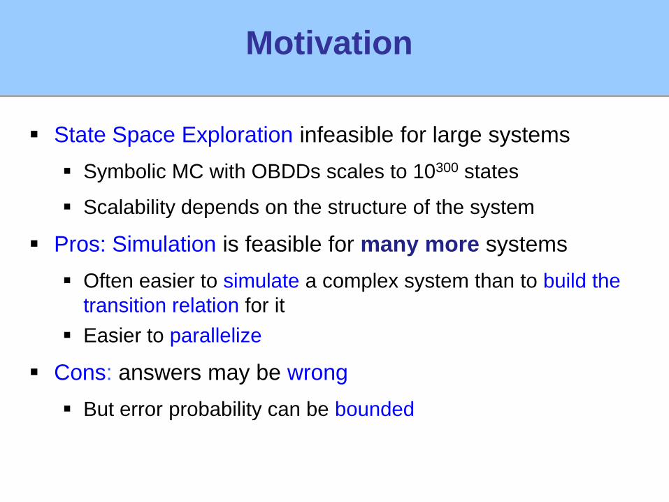
State Space Exploration infeasible for large systems

Symbolic MC with OBDDs scales to 10300 states

Scalability depends on the structure of the system

Pros: Simulation is feasible for many more systems

Often easier to simulate a complex system than to build the

transition relation for it

Easier to parallelize

Cons: answers may be wrong

But error probability can be bounded

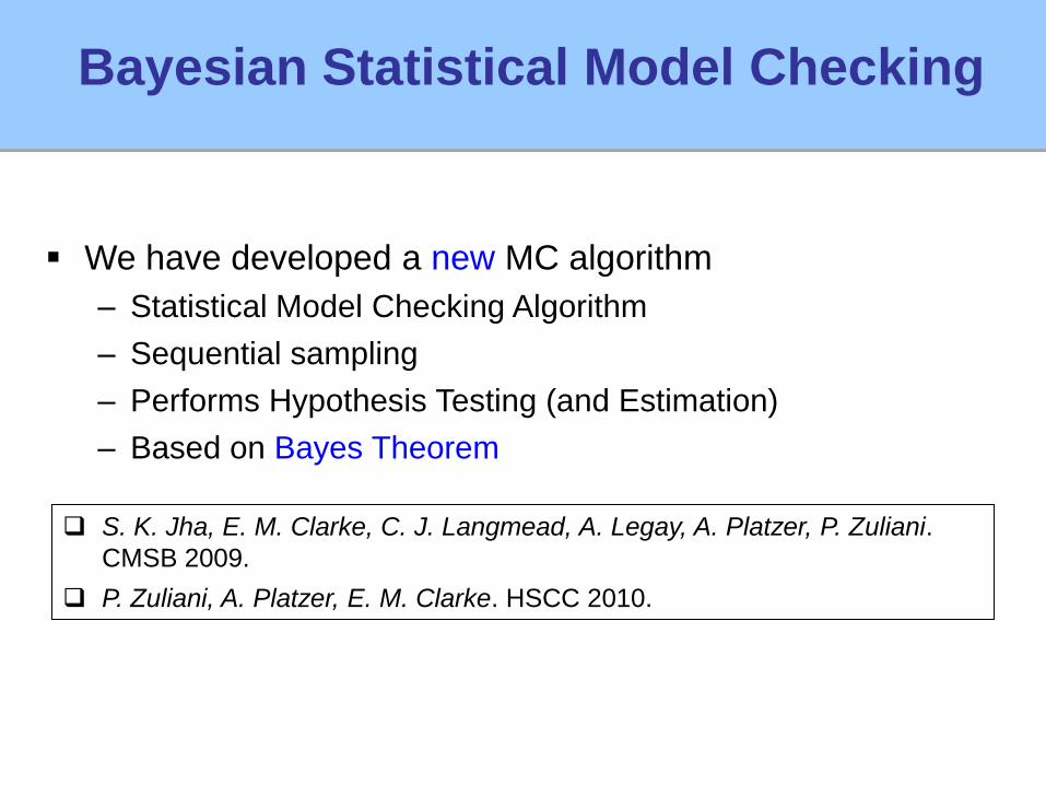
We have developed a new MC algorithm

– Statistical Model Checking Algorithm

– Sequential sampling

– Performs Hypothesis Testing (and Estimation)

– Based on Bayes Theorem

Bayesian Statistical Model Checking

S. K. Jha, E. M. Clarke, C. J. Langmead, A. Legay, A. Platzer, P. Zuliani.

CMSB 2009.

P. Zuliani, A. Platzer, E. M. Clarke. HSCC 2010.

Bayesian Statistics

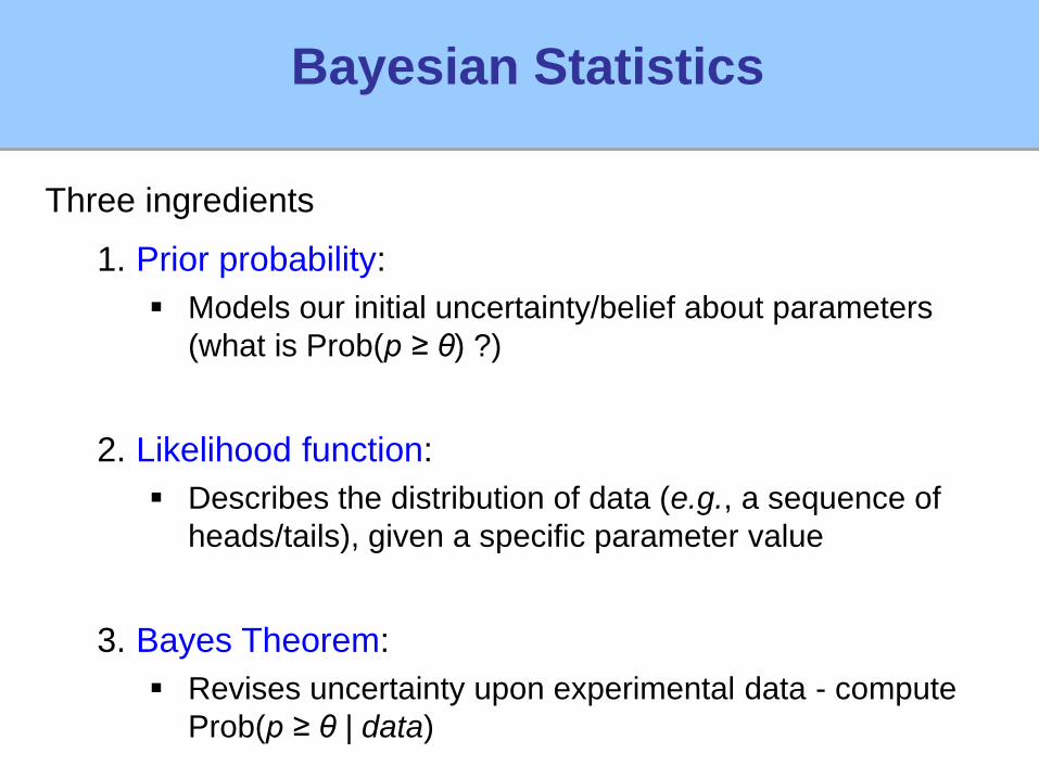
Three ingredients

1. Prior probability:

Models our initial uncertainty/belief about parameters

(what is Prob(p ≥ θ) ?)

2. Likelihood function:

Describes the distribution of data (e.g., a sequence of

heads/tails), given a specific parameter value

3. Bayes Theorem:

Revises uncertainty upon experimental data - compute

Prob(p ≥ θ | data)

Bounded Linear Temporal Logic

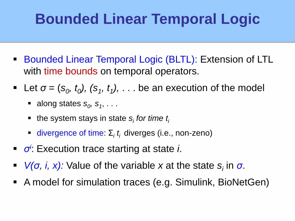
Bounded Linear Temporal Logic (BLTL): Extension of LTL

with time bounds on temporal operators.

Let σ = (s0, t0), (s1, t1), . . . be an execution of the model

along states s0, s1, . . .

the system stays in state si for time ti

divergence of time: Σi ti diverges (i.e., non-zeno)

σi: Execution trace starting at state i.

V(σ, i, x): Value of the variable x at the state si in σ.

A model for simulation traces (e.g. Simulink, BioNetGen)

Semantics of BLTL

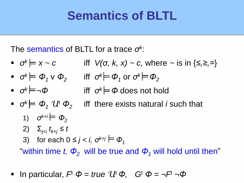
The semantics of BLTL for a trace σk:

σk x ~ c iff V(σ, k, x) ~ c, where ~ is in {≤,≥,=}

σk Φ1 v Φ2 iff σk Φ1 or σk Φ2

σk ¬Φ iff σk Φ does not hold

σk Φ1 Ut Φ2 iff there exists natural i such that

1) σk+i Φ2

2) Σj<i tk+j ≤ t

3) for each 0 ≤ j < i, σk+j Φ1

“within time t, Φ2 will be true and Φ1 will hold until then”

In particular, Ft Φ = true Ut Φ, Gt Φ = ¬Ft ¬Φ

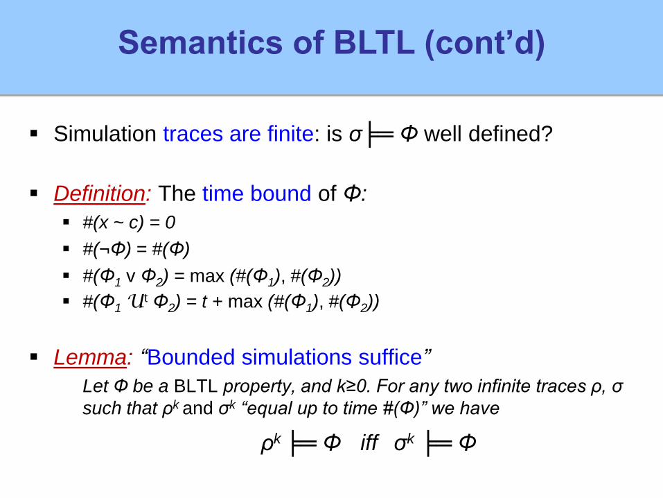
Simulation traces are finite: is σ╞═ Φ well defined?

Definition: The time bound of Φ:

#(x ~ c) = 0

#(¬Φ) = #(Φ)

#(Φ1 v Φ2) = max (#(Φ1), #(Φ2))

#(Φ1 Ut Φ2) = t + max (#(Φ1), #(Φ2))

Lemma: “Bounded simulations suffice”

Let Ф be a BLTL property, and k≥0. For any two infinite traces ρ, σ

such that ρk and σk “equal up to time #(Ф)” we have

ρk ╞═ Φ iff σk ╞═ Φ

Semantics of BLTL (cont’d)

Sequential Bayesian Statistical MC - I

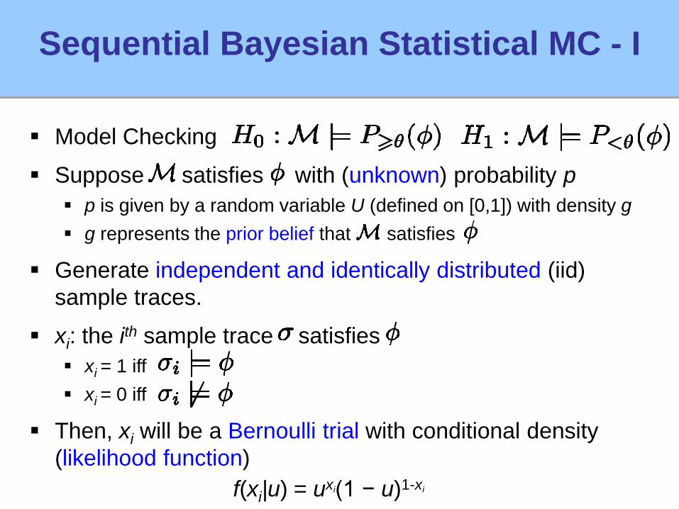
Model Checking

Suppose satisfies with (unknown) probability p

p is given by a random variable U (defined on [0,1]) with density g

g represents the prior belief that satisfies

Generate independent and identically distributed (iid)

sample traces.

xi: the ith sample trace satisfies

xi = 1 iff

xi = 0 iff

Then, xi will be a Bernoulli trial with conditional density

(likelihood function)

f(xi|u) = uxi(1 − u)1-xi

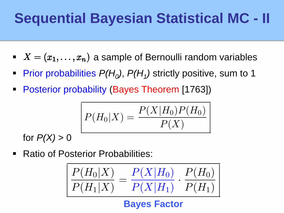
a sample of Bernoulli random variables

Prior probabilities P(H0), P(H1) strictly positive, sum to 1

Posterior probability (Bayes Theorem [1763])

for P(X) > 0

Ratio of Posterior Probabilities:

Bayes Factor

Sequential Bayesian Statistical MC - II

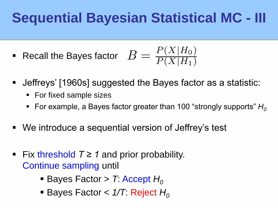
Sequential Bayesian Statistical MC - III

Recall the Bayes factor

Jeffreys’ [1960s] suggested the Bayes factor as a statistic:

For fixed sample sizes

For example, a Bayes factor greater than 100 “strongly supports” H0

We introduce a sequential version of Jeffrey’s test

Fix threshold T ≥ 1 and prior probability.

Continue sampling until

Bayes Factor > T: Accept H0

Bayes Factor < 1/T: Reject H0

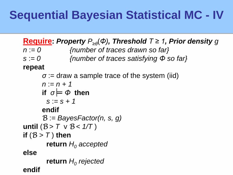
Require: Property P≥θ(Φ), Threshold T ≥ 1, Prior density g

n := 0 {number of traces drawn so far}

s := 0 {number of traces satisfying Φ so far}

repeat

σ := draw a sample trace of the system (iid)

n := n + 1

if σ Φ then

s := s + 1

endifB := BayesFactor(n, s, g)

until (B > T v B < 1/T )

if (B > T ) then

return H0 accepted

else

return H0 rejected

endif

Sequential Bayesian Statistical MC - IV

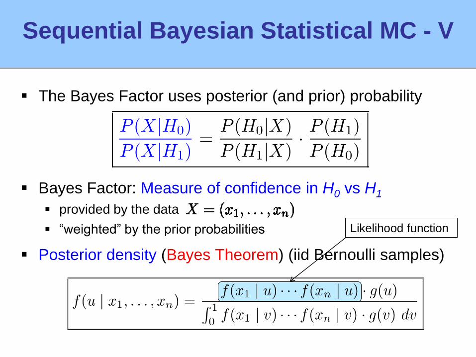
The Bayes Factor uses posterior (and prior) probability

Bayes Factor: Measure of confidence in H0 vs H1

provided by the data

“weighted” by the prior probabilities

Posterior density (Bayes Theorem) (iid Bernoulli samples)

07/16/0907/16/0907/16/0907/16/0907/16/0907/16/09

Sequential Bayesian Statistical MC - V

Likelihood function

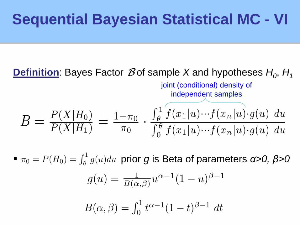
Sequential Bayesian Statistical MC - VI

Definition: Bayes Factor B of sample X and hypotheses H0, H1

prior g is Beta of parameters α>0, β>0

joint (conditional) density of

independent samples

07/16/0907/16/0907/16/0907/16/0907/16/0907/16/09

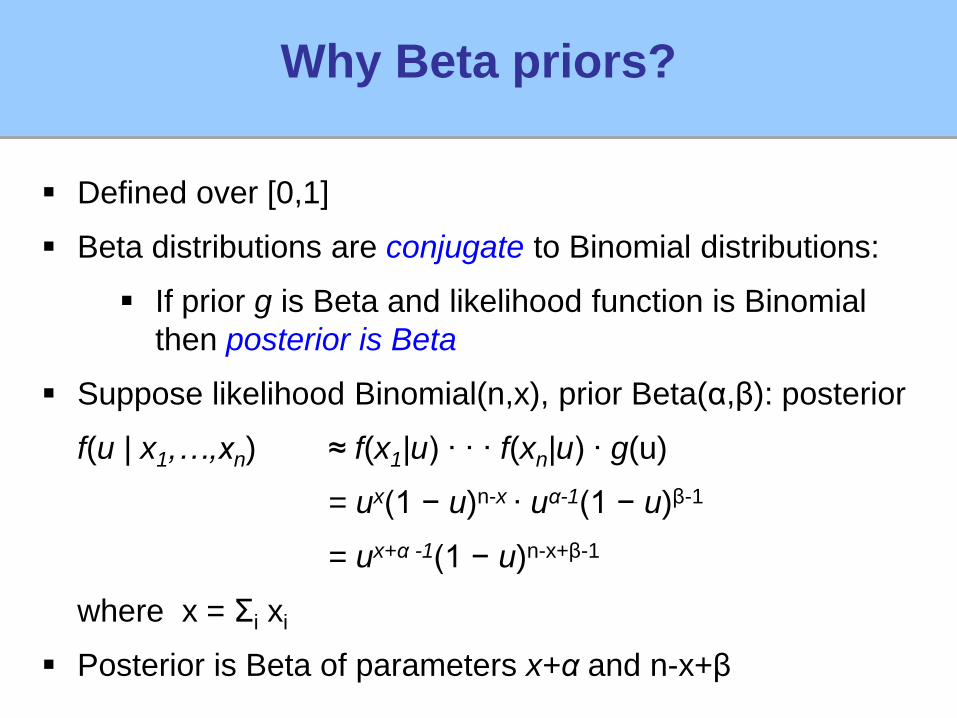
Why Beta priors?

Defined over [0,1]

Beta distributions are conjugate to Binomial distributions:

If prior g is Beta and likelihood function is Binomial

then posterior is Beta

Suppose likelihood Binomial(n,x), prior Beta(α,β): posterior

f(u | x1,…,xn) ≈ f(x1|u) ∙ ∙ ∙ f(xn|u) ∙ g(u)

= ux(1 − u)n-x ∙ uα-1(1 − u)β-1

= ux+α -1(1 − u)n-x+β-1

where x = Σi xi

Posterior is Beta of parameters x+α and n-x+β

0 0.1 0.2 0.3 0.4 0.5 0.6 0.7 0.8 0.9 10.5

1

1.5

2

2.5

3

3.5

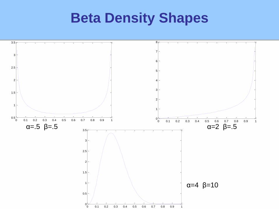
α=.5 β=.5 0 0.1 0.2 0.3 0.4 0.5 0.6 0.7 0.8 0.9 1

0

1

2

3

4

5

6

7

8

α=2 β=.5

0 0.1 0.2 0.3 0.4 0.5 0.6 0.7 0.8 0.9 10

0.5

1

1.5

2

2.5

3

3.5

α=4 β=10

Beta Density Shapes

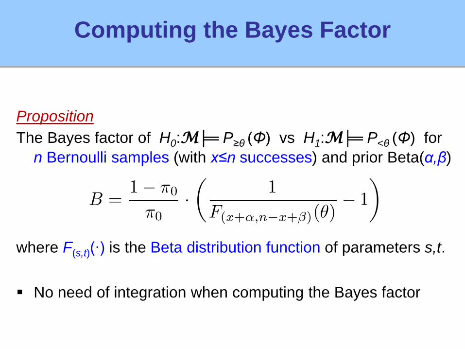
Proposition

The Bayes factor of H0:M╞═ P≥θ (Φ) vs H1:M╞═ P<θ (Φ) for

n Bernoulli samples (with x≤n successes) and prior Beta(α,β)

where F(s,t)(∙) is the Beta distribution function of parameters s,t.

No need of integration when computing the Bayes factor

Computing the Bayes Factor

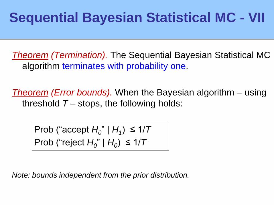
Theorem (Termination). The Sequential Bayesian Statistical MC

algorithm terminates with probability one.

Theorem (Error bounds). When the Bayesian algorithm – using

threshold T – stops, the following holds:

Prob (“accept H0” | H1) ≤ 1/T

Prob (“reject H0” | H0) ≤ 1/T

Note: bounds independent from the prior distribution.

Sequential Bayesian Statistical MC - VII

Fuel Control System - I

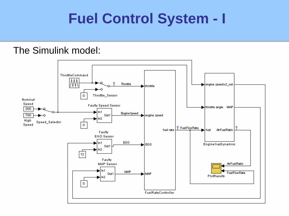
The Simulink model:

Fuel Control System - II

Ratio between air mass flow rate and fuel mass flow rate

Stoichometric ratio is 14.6

Senses amount of oxygen in exhaust gas, pressure,

engine speed and throttle to compute correct fuel rate.

Single sensor faults are compensated by switching to a higher

oxygen content mixture.

Multiple sensor faults force engine shutdown.

07/16/09

Fuel Control System - III

Stateflow part of the model has 24 locations

grouped in 6 simultaneously active states

Simulink part of the model is rich

Several nonlinear equations

Linear ODE

Probabilistic behavior because of random faults

in the EGO (oxygen), pressure and speed sensors.

Faults modeled by three independent Poisson processes

We did not change the speed or throttle inputs.

07/16/09

Fuel Control System - IV

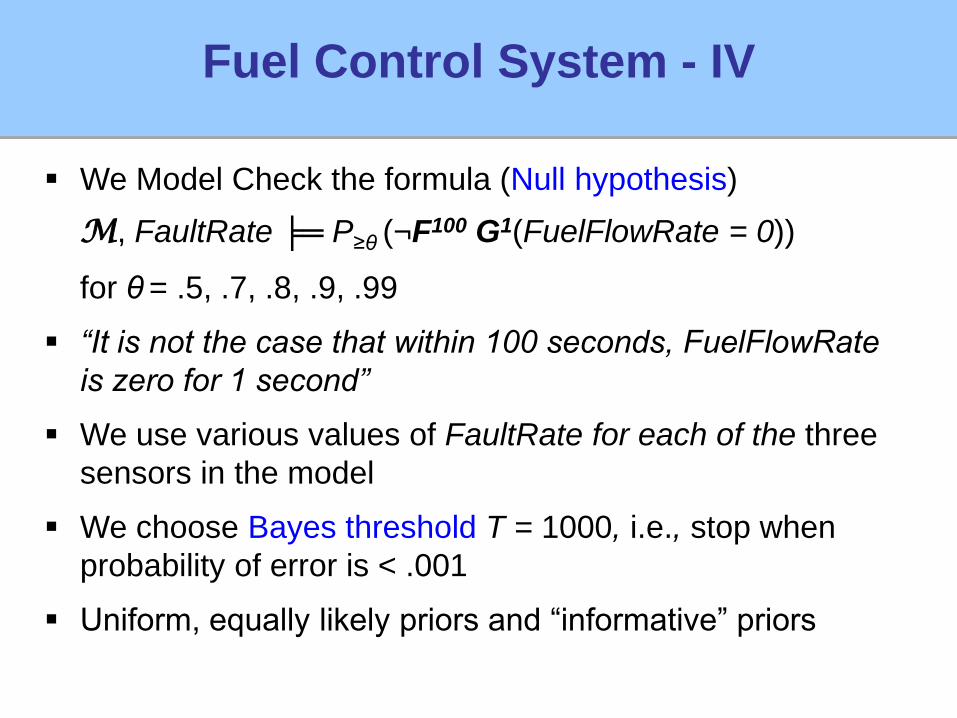
We Model Check the formula (Null hypothesis)

M, FaultRate ╞═ P≥θ (¬F100 G1(FuelFlowRate = 0))

for θ = .5, .7, .8, .9, .99

“It is not the case that within 100 seconds, FuelFlowRate

is zero for 1 second”

We use various values of FaultRate for each of the three

sensors in the model

We choose Bayes threshold T = 1000, i.e., stop when

probability of error is < .001

Uniform, equally likely priors and “informative” priors

Fuel Control System: results

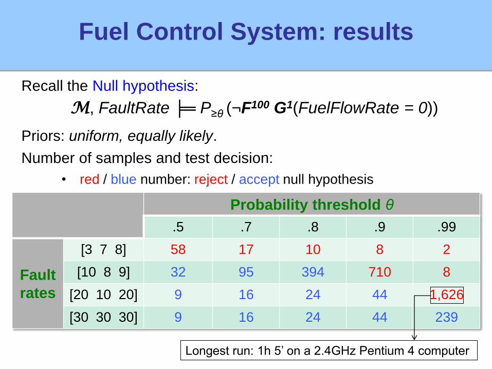
Recall the Null hypothesis:

M, FaultRate ╞═ P≥θ (¬F100 G1(FuelFlowRate = 0))

Priors: uniform, equally likely.

Number of samples and test decision:

• red / blue number: reject / accept null hypothesis

Probability threshold θ

.5 .7 .8 .9 .99

Fault

rates

[3 7 8] 58 17 10 8 2

[10 8 9] 32 95 394 710 8

[20 10 20] 9 16 24 44 1,626

[30 30 30] 9 16 24 44 239

Longest run: 1h 5’ on a 2.4GHz Pentium 4 computer

07/16/0907/16/0907/16/0907/16/0907/16/0907/16/09

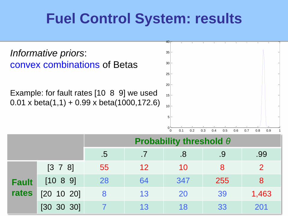
Fuel Control System: results

Probability threshold θ

.5 .7 .8 .9 .99

Fault

rates

[3 7 8] 55 12 10 8 2

[10 8 9] 28 64 347 255 8

[20 10 20] 8 13 20 39 1,463

[30 30 30] 7 13 18 33 201

0 0.1 0.2 0.3 0.4 0.5 0.6 0.7 0.8 0.9 10

5

10

15

20

25

30

35

40

Informative priors:

convex combinations of Betas

Example: for fault rates [10 8 9] we used

0.01 x beta(1,1) + 0.99 x beta(1000,172.6)

07/16/0907/16/0907/16/0907/16/0907/16/0907/16/09

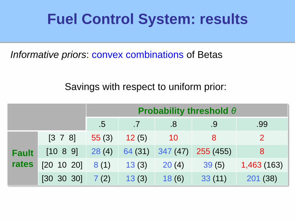
Fuel Control System: results

Probability threshold θ

.5 .7 .8 .9 .99

Fault

rates

[3 7 8] 55 (3) 12 (5) 10 8 2

[10 8 9] 28 (4) 64 (31) 347 (47) 255 (455) 8

[20 10 20] 8 (1) 13 (3) 20 (4) 39 (5) 1,463 (163)

[30 30 30] 7 (2) 13 (3) 18 (6) 33 (11) 201 (38)

Informative priors: convex combinations of Betas

Savings with respect to uniform prior:

CMACS interactions

Verification of Pancreatic Cancer models:

James Faeder and Haijun Gong (tomorrow)

Rule-based models

Full integration of BLTL trace verifier with BioNetGen

Can use Statistical Model Checking

Probabilistic Boolean Network models

Work in progress

Atrial fibrillation (Flavio Fenton et al.)

CMACS interactions

Hybrid Systems:

Embed BLTL checker in Simulink

Run-time verification (Klaus Havelund)

Requirements in automotive (Rance Cleveland)

Theory: stochastic hybrid systems (Steve Marcus)

Rare event simulation, nondeterminism

Model Checking: abstraction (Patrick Cousot)

Speed-up simulation while preserving temporal logic

properties

The End

Questions?

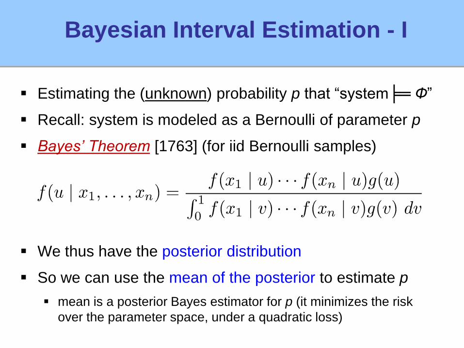
Bayesian Interval Estimation - I

Estimating the (unknown) probability p that “system╞═ Ф”

Recall: system is modeled as a Bernoulli of parameter p

Bayes’ Theorem [1763] (for iid Bernoulli samples)

We thus have the posterior distribution

So we can use the mean of the posterior to estimate p

mean is a posterior Bayes estimator for p (it minimizes the risk

over the parameter space, under a quadratic loss)

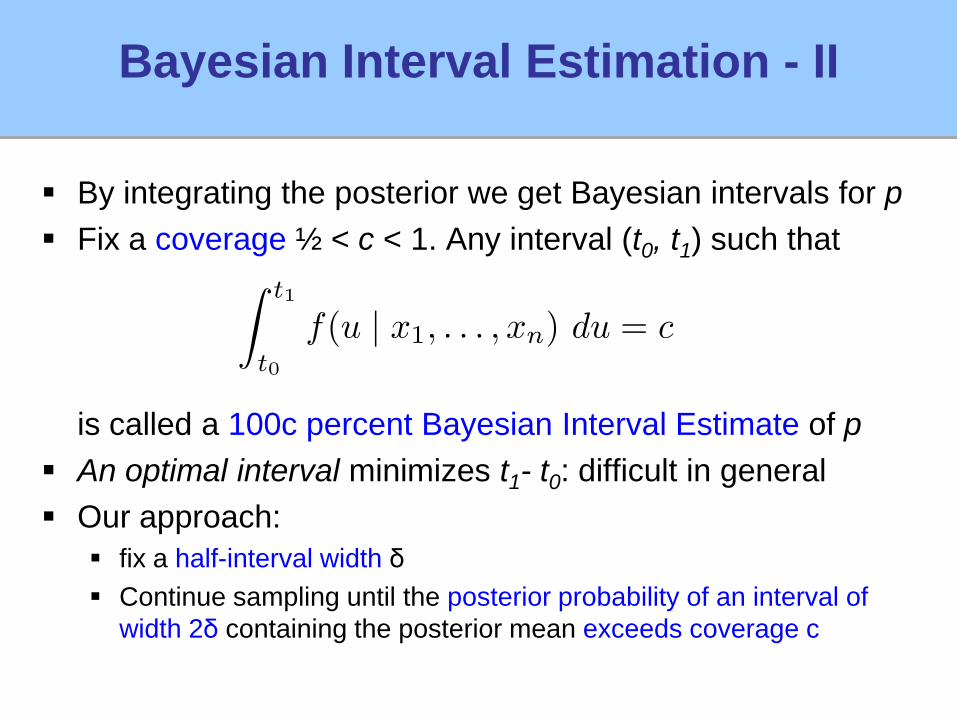
By integrating the posterior we get Bayesian intervals for p

Fix a coverage ½ < c < 1. Any interval (t0, t1) such that

is called a 100c percent Bayesian Interval Estimate of p

An optimal interval minimizes t1- t0: difficult in general

Our approach:

fix a half-interval width δ

Continue sampling until the posterior probability of an interval of

width 2δ containing the posterior mean exceeds coverage c

Bayesian Interval Estimation - II

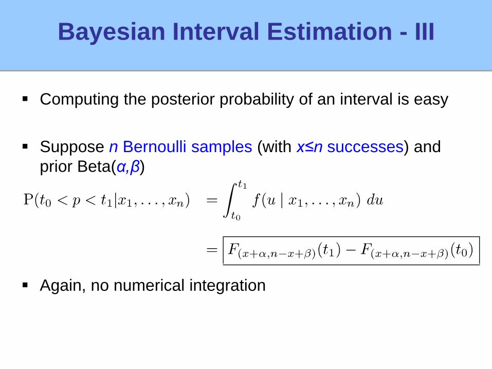
Computing the posterior probability of an interval is easy

Suppose n Bernoulli samples (with x≤n successes) and

prior Beta(α,β)

Again, no numerical integration

Bayesian Interval Estimation - III

0 0.1 0.2 0.3 0.4 0.5 0.6 0.7 0.8 0.9 10

5

10

15

20

25

30

35

40

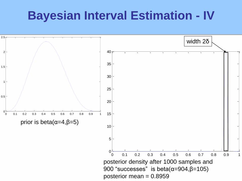
Bayesian Interval Estimation - IV

0 0.1 0.2 0.3 0.4 0.5 0.6 0.7 0.8 0.9 10

0.5

1

1.5

2

2.5

prior is beta(α=4,β=5)

posterior density after 1000 samples and

900 “successes” is beta(α=904,β=105)

posterior mean = 0.8959

width 2δ

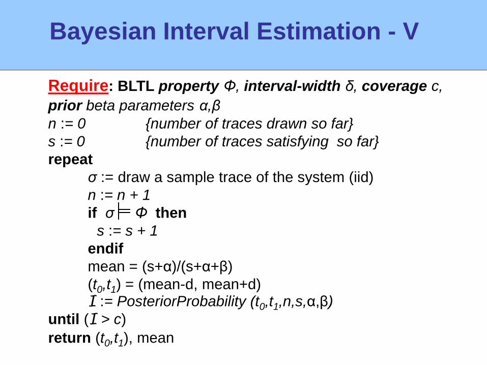
Require: BLTL property Φ, interval-width δ, coverage c,

prior beta parameters α,β

n := 0 {number of traces drawn so far}

s := 0 {number of traces satisfying so far}

repeat

σ := draw a sample trace of the system (iid)

n := n + 1

if σ Φ then

s := s + 1

endif

mean = (s+α)/(s+α+β)

(t0,t1) = (mean-d, mean+d)I := PosteriorProbability (t0,t1,n,s,α,β)

until (I > c)

return (t0,t1), mean

Bayesian Interval Estimation - V

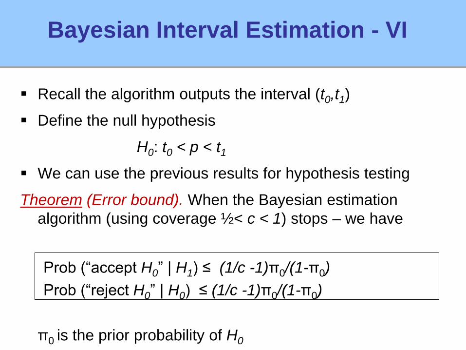
Recall the algorithm outputs the interval (t0,t1)

Define the null hypothesis

H0: t0 < p < t1

We can use the previous results for hypothesis testing

Theorem (Error bound). When the Bayesian estimation

algorithm (using coverage ½< c < 1) stops – we have

Prob (“accept H0” | H1) ≤ (1/c -1)π0/(1-π0)

Prob (“reject H0” | H0) ≤ (1/c -1)π0/(1-π0)

π0 is the prior probability of H0

Bayesian Interval Estimation - VI

07/16/0907/16/0907/16/0907/16/0907/16/0907/16/09

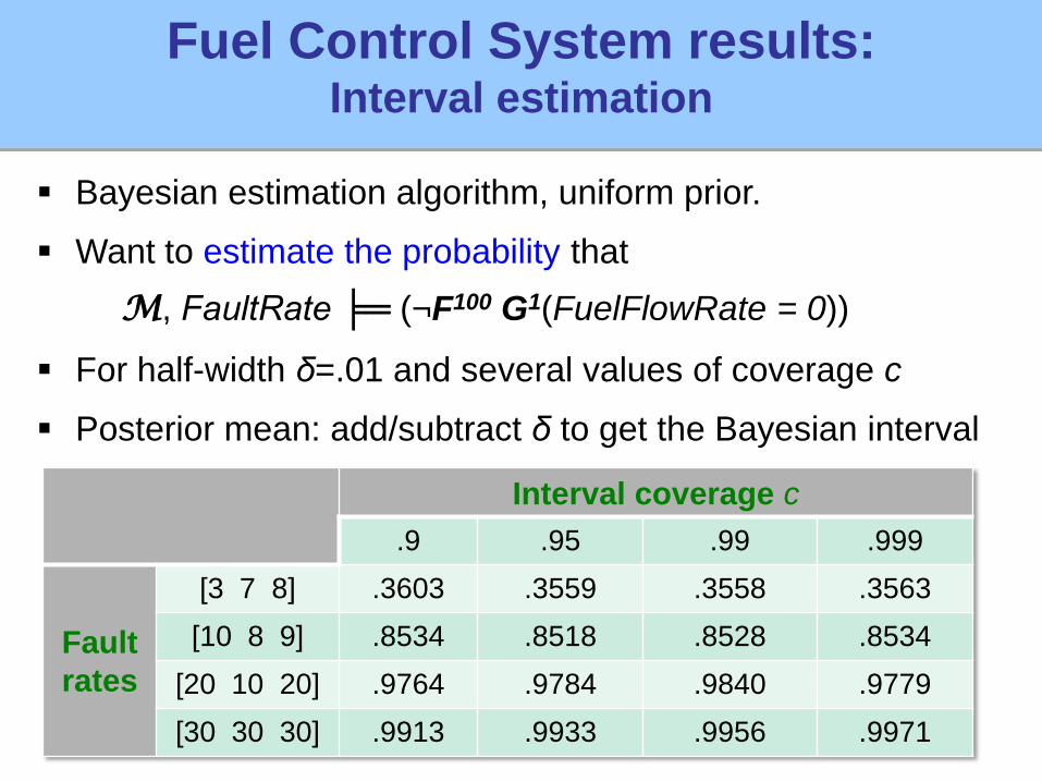
Fuel Control System results:Interval estimation

Interval coverage c

.9 .95 .99 .999

Fault

rates

[3 7 8] .3603 .3559 .3558 .3563

[10 8 9] .8534 .8518 .8528 .8534

[20 10 20] .9764 .9784 .9840 .9779

[30 30 30] .9913 .9933 .9956 .9971

Bayesian estimation algorithm, uniform prior.

Want to estimate the probability that

M, FaultRate ╞═ (¬F100 G1(FuelFlowRate = 0))

For half-width δ=.01 and several values of coverage c

Posterior mean: add/subtract δ to get the Bayesian interval

07/16/0907/16/0907/16/0907/16/0907/16/0907/16/09

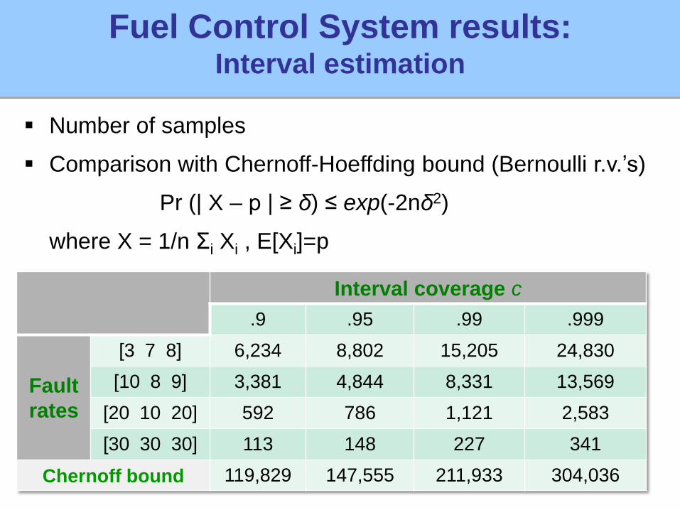
Interval coverage c

.9 .95 .99 .999

Fault

rates

[3 7 8] 6,234 8,802 15,205 24,830

[10 8 9] 3,381 4,844 8,331 13,569

[20 10 20] 592 786 1,121 2,583

[30 30 30] 113 148 227 341

Chernoff bound 119,829 147,555 211,933 304,036

Number of samples

Comparison with Chernoff-Hoeffding bound (Bernoulli r.v.’s)

Pr (| X – p | ≥ δ) ≤ exp(-2nδ2)

where X = 1/n Σi Xi , E[Xi]=p

Fuel Control System results:Interval estimation

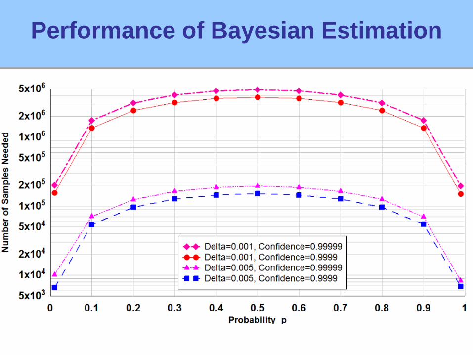
Performance of Bayesian Estimation

07/16/09

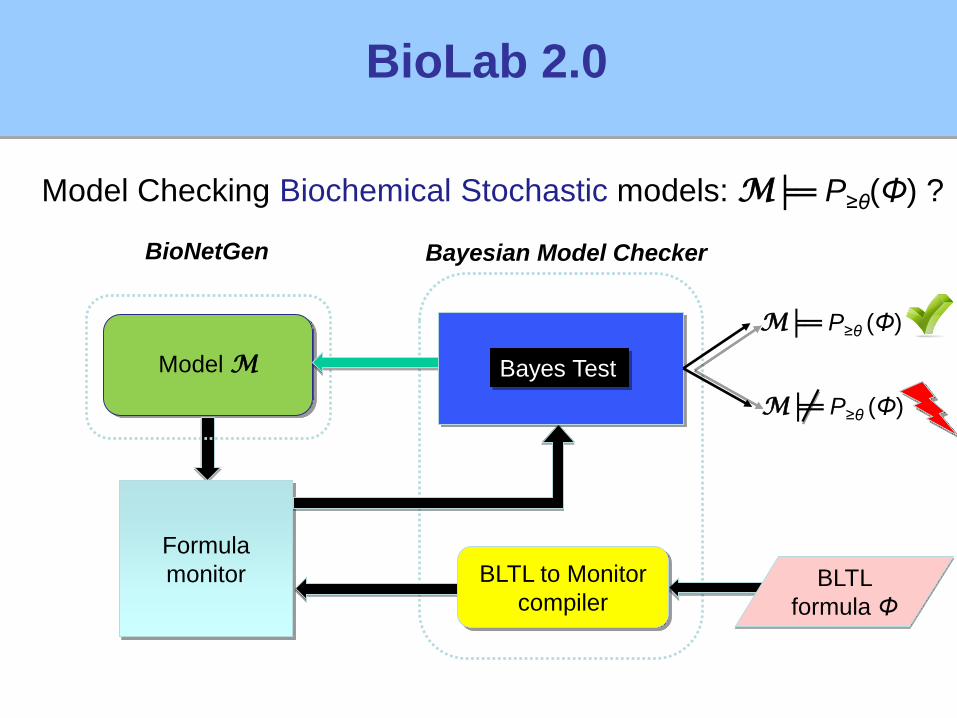
BioLab 2.0

Model Checking Biochemical Stochastic models: M╞═ P≥θ(Φ) ?

Model M

BioNetGen Bayesian Model Checker

BLTL

formula Φ

BLTL to Monitor

compiler

Formula

monitor

M╞═ P≥θ (Φ)

Bayes Test

M╞═ P≥θ (Φ)