bayesian analysis of multinomial n-mixture models in · pdf filebayesian analysis of...
TRANSCRIPT

Bayesian Analysis of Multinomial N-mixture models in BUGS
Multinomial N-mixture in BUGS
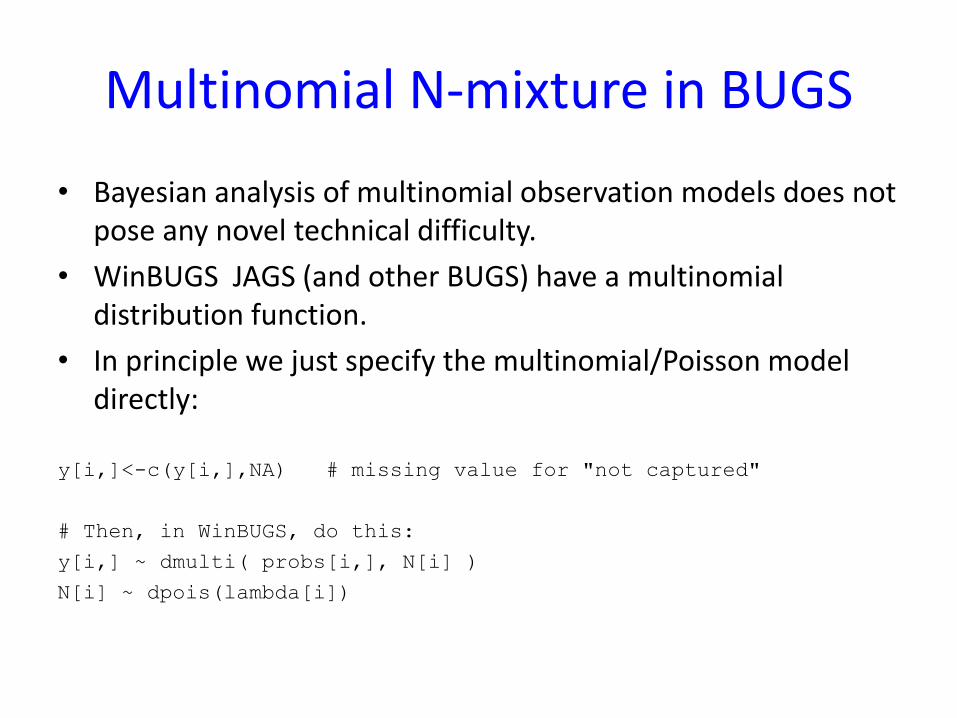
• Bayesian analysis of multinomial observation models does not pose any novel technical difficulty.
• WinBUGS JAGS (and other BUGS) have a multinomial distribution function.
• In principle we just specify the multinomial/Poisson model directly:
y[i,]<-c(y[i,],NA) # missing value for "not captured"
# Then, in WinBUGS, do this:
y[i,] ~ dmulti( probs[i,], N[i] )
N[i] ~ dpois(lambda[i])
Multinomial N-mixture in BUGS
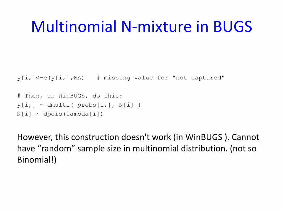
y[i,]<-c(y[i,],NA) # missing value for "not captured"
# Then, in WinBUGS, do this:
y[i,] ~ dmulti( probs[i,], N[i] )
N[i] ~ dpois(lambda[i])
However, this construction doesn't work (in WinBUGS ). Cannot have “random” sample size in multinomial distribution. (not so Binomial!)
Approaches to Bayesian analysis
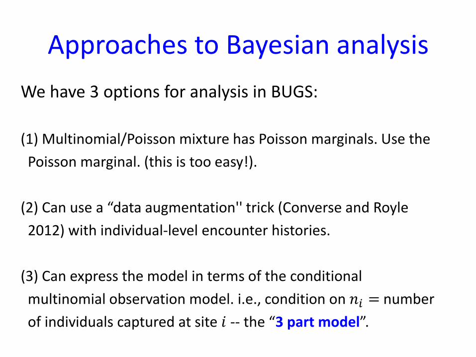
We have 3 options for analysis in BUGS:
(1) Multinomial/Poisson mixture has Poisson marginals. Use the
Poisson marginal. (this is too easy!).
(2) Can use a “data augmentation'' trick (Converse and Royle
2012) with individual-level encounter histories.
(3) Can express the model in terms of the conditional
multinomial observation model. i.e., condition on 𝑛𝑖 = number
of individuals captured at site 𝑖 -- the “3 part model”.
Topics in Bayesian analysis
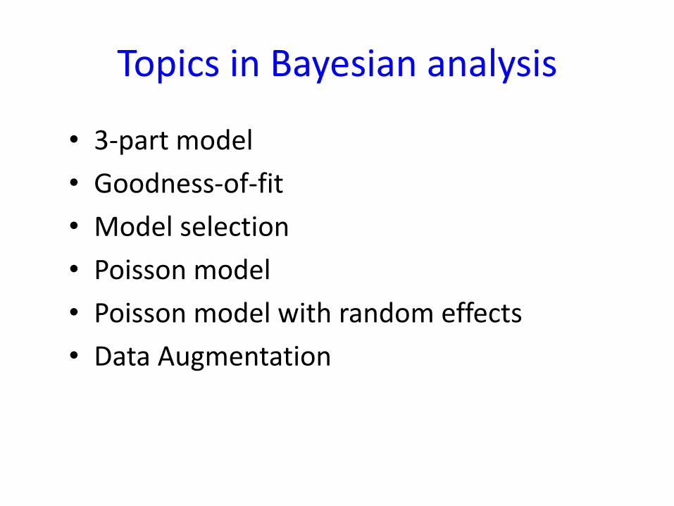
• 3-part model
• Goodness-of-fit
• Model selection
• Poisson model
• Poisson model with random effects
• Data Augmentation
The 3-part (conditional multinomial) model
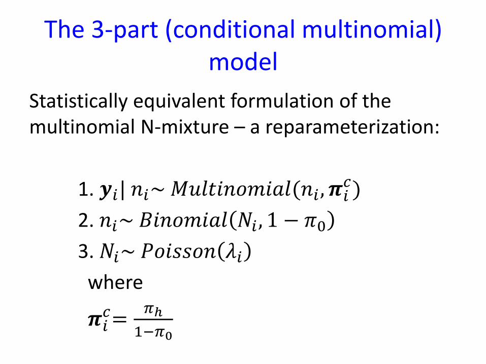
Statistically equivalent formulation of the multinomial N-mixture – a reparameterization:
1. 𝒚𝑖| 𝑛𝑖~ 𝑀𝑢𝑙𝑡𝑖𝑛𝑜𝑚𝑖𝑎𝑙(𝑛𝑖 , 𝝅𝑖𝑐)
2. 𝑛𝑖~ 𝐵𝑖𝑛𝑜𝑚𝑖𝑎𝑙 𝑁𝑖 , 1 − 𝜋0
3. 𝑁𝑖~ 𝑃𝑜𝑖𝑠𝑠𝑜𝑛 𝜆𝑖
where
𝝅𝑖𝑐=
𝜋ℎ
1−𝜋0

model {
# Prior distributions
p0 ~ dunif(0,1)
alpha0 <- logit(p0)
alpha1 ~ dnorm(0, 0.01)
beta0 ~ dnorm(0, 0.01)
beta1 ~ dnorm(0, 0.01)
beta2 ~ dnorm(0, 0.01)
beta3 ~ dnorm(0, 0.01)
for(i in 1:M){ # Loop over sites
# Conditional multinomial cell probabilities
pi[i,1] <- p[i]
pi[i,2] <- p[i]*(1-p[i])
pi[i,3] <- p[i]*(1-p[i])*(1-p[i])
pi[i,4] <- p[i]*(1-p[i])*(1-p[i])*(1-p[i])
pi0[i] <- 1 - (pi[i,1] + pi[i,2] + pi[i,3] + pi[i,4])
pcap[i] <- 1 - pi0[i]
for(j in 1:4){
pic[i,j] <- pi[i,j] / pcap[i]
}
# logit-linear model for detection: understory cover effect
logit(p[i]) <- alpha0 + alpha1 * X[i,1]
# Model specification, three parts:
y[i,1:4] ~ dmulti(pic[i,1:4], n[i]) # component 1 uses the
# conditional cell probabilities
n[i] ~ dbin(pcap[i], N[i]) # component 2 is a model
# for the observed sample size
N[i] ~ dpois(lambda[i]) # part 3 is the process model
# log-linear model for abundance: UFC + TRBA + UFC:TRBA
log(lambda[i])<- beta0 + beta1*X[i,1] + beta2*X[i,2] + beta3*X[i,2]*X[i,1]
}
}
Have to write out the cell probabilities explicitly
Goodness-of-fit Using Bayesian p-values
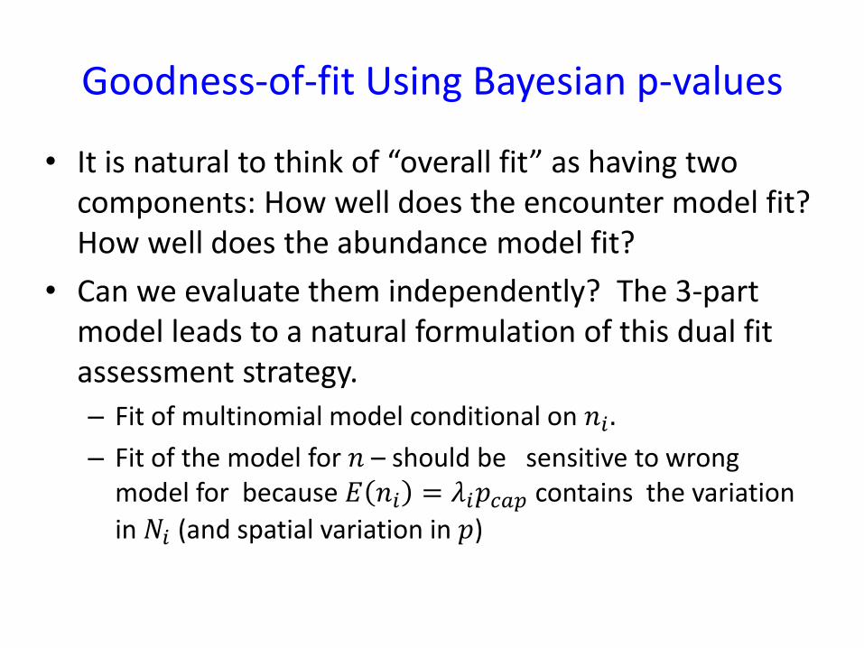
• It is natural to think of “overall fit” as having two components: How well does the encounter model fit? How well does the abundance model fit?
• Can we evaluate them independently? The 3-part model leads to a natural formulation of this dual fit assessment strategy.
– Fit of multinomial model conditional on 𝑛𝑖 .
– Fit of the model for 𝑛 – should be sensitive to wrong model for because 𝐸 𝑛𝑖 = 𝜆𝑖𝑝𝑐𝑎𝑝 contains the variation
in 𝑁𝑖 (and spatial variation in 𝑝)

Implementation of 2-part GoF idea
for(i in 1:nsites){
ncap.fit[i] ~ dbin(pcap[i],N[i])
y.fit[i,1:4] ~ dmulti(muc[i,1:4],ncap[i])
for(t in 1:4){
e1[i,t]<- muc[i,t]*ncap[i] # Expected value
resid1[i,t]<- pow(pow(y[i,t],0.5)-pow(e1[i,t],0.5),2)
resid1.fit[i,t]<- pow(pow(y.fit[i,t],0.5) - pow(e1[i,t],0.5),2)
}
e2[i]<- pcap[i]*lambda[i] # Expected value
resid2[i]<- pow( pow(ncap[i],0.5) - pow(e2[i],0.5),2)
resid2.fit[i]<- pow( pow(ncap.fit[i],0.5) - pow(e2[i],0.5),2)
}
fit1.data<- sum(resid1[,])
fit1.post<- sum(resid1.fit[,])
fit2.data<- sum(resid2[])
fit2.post<- sum(resid2.fit[])
Goodness-of-fit Using Bayesian p-values
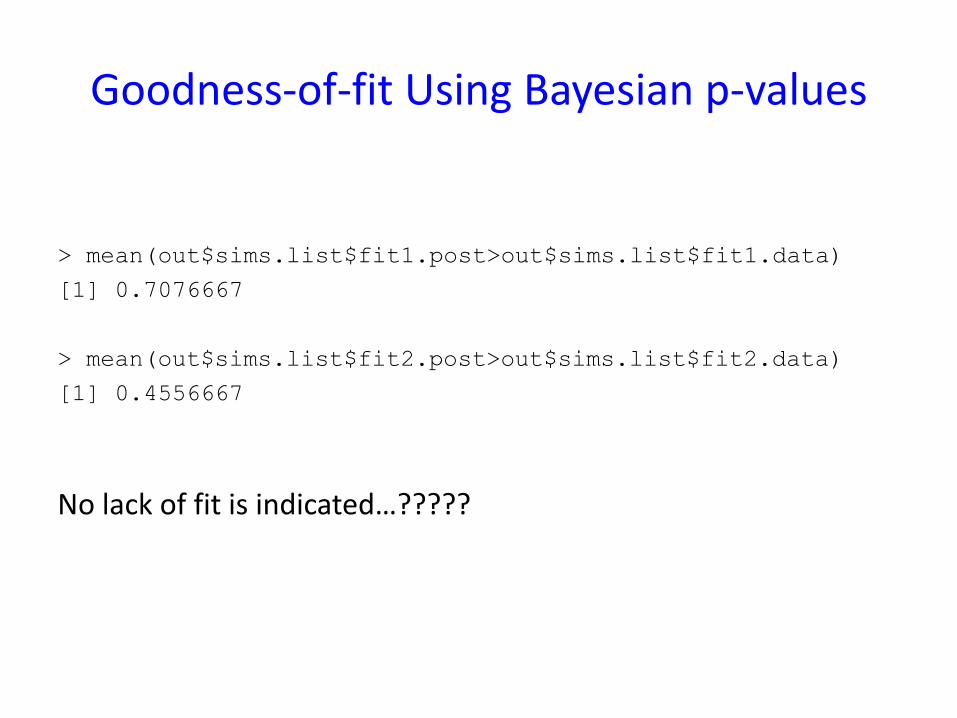
> mean(out$sims.list$fit1.post>out$sims.list$fit1.data)
[1] 0.7076667
> mean(out$sims.list$fit2.post>out$sims.list$fit2.data)
[1] 0.4556667
No lack of fit is indicated…?????

Goodness-of-fit: Research Question
The power of any particular fit statistic to any particular departure from the model is unknown and no studies have been published.
Model Selection in BUGS: Computing posterior model probabilities
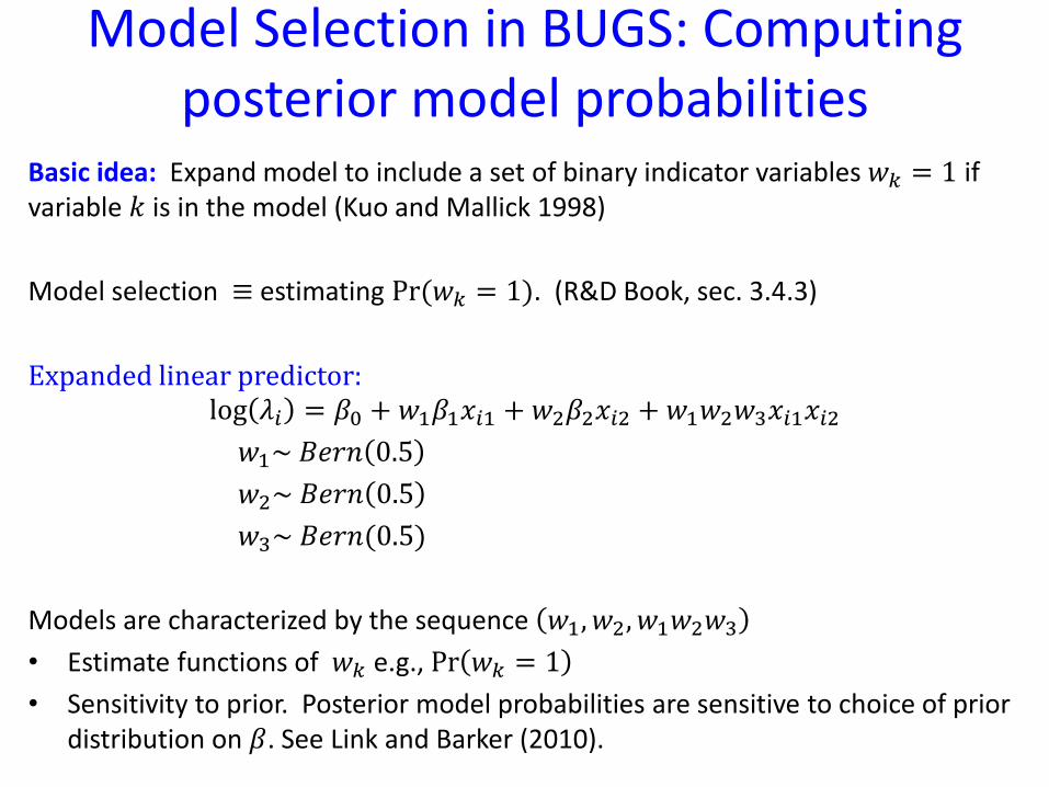
Basic idea: Expand model to include a set of binary indicator variables 𝑤𝑘 = 1 if variable 𝑘 is in the model (Kuo and Mallick 1998)
Model selection ≡ estimating Pr (𝑤𝑘 = 1). (R&D Book, sec. 3.4.3)
Expanded linear predictor: log 𝜆𝑖 = 𝛽0 + 𝑤1𝛽1𝑥𝑖1 + 𝑤2𝛽2𝑥𝑖2 + 𝑤1𝑤2𝑤3𝑥𝑖1𝑥𝑖2
𝑤1~ 𝐵𝑒𝑟𝑛 0.5
𝑤2~ 𝐵𝑒𝑟𝑛 0.5
𝑤3~ 𝐵𝑒𝑟𝑛(0.5)
Models are characterized by the sequence 𝑤1, 𝑤2, 𝑤1𝑤2𝑤3
• Estimate functions of 𝑤𝑘 e.g., Pr 𝑤𝑘 = 1
• Sensitivity to prior. Posterior model probabilities are sensitive to choice of prior distribution on 𝛽. See Link and Barker (2010).
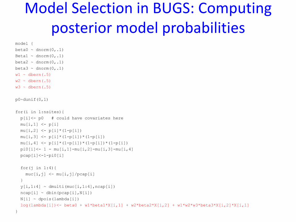
Model Selection in BUGS: Computing posterior model probabilities
model {
beta0 ~ dnorm(0,.1)
Beta1 ~ dnorm(0,.1)
beta2 ~ dnorm(0,.1)
beta3 ~ dnorm(0,.1)
w1 ~ dbern(.5)
w2 ~ dbern(.5)
w3 ~ dbern(.5)
p0~dunif(0,1)
for(i in 1:nsites){
p[i]<- p0 # could have covariates here
mu[i,1] <- p[i]
mu[i,2] <- p[i]*(1-p[i])
mu[i,3] <- p[i]*(1-p[i])*(1-p[i])
mu[i,4] <- p[i]*(1-p[i])*(1-p[i])*(1-p[i])
pi0[i]<- 1 - mu[i,1]-mu[i,2]-mu[i,3]-mu[i,4]
pcap[i]<-1-pi0[i]
for(j in 1:4){
muc[i,j] <- mu[i,j]/pcap[i]
}
y[i,1:4] ~ dmulti(muc[i,1:4],ncap[i])
ncap[i] ~ dbin(pcap[i],N[i])
N[i] ~ dpois(lambda[i])
log(lambda[i])<- beta0 + w1*beta1*X[i,1] + w2*beta2*X[i,2] + w1*w2*w3*beta3*X[i,2]*X[i,1]
}
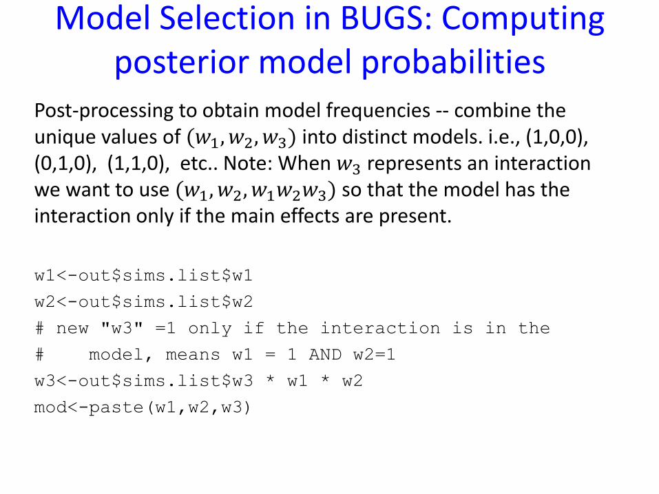
Model Selection in BUGS: Computing posterior model probabilities
Post-processing to obtain model frequencies -- combine the unique values of (𝑤1, 𝑤2, 𝑤3) into distinct models. i.e., (1,0,0), (0,1,0), (1,1,0), etc.. Note: When 𝑤3 represents an interaction we want to use (𝑤1, 𝑤2, 𝑤1𝑤2𝑤3) so that the model has the interaction only if the main effects are present.
w1<-out$sims.list$w1
w2<-out$sims.list$w2
# new "w3" =1 only if the interaction is in the
# model, means w1 = 1 AND w2=1
w3<-out$sims.list$w3 * w1 * w2
mod<-paste(w1,w2,w3)
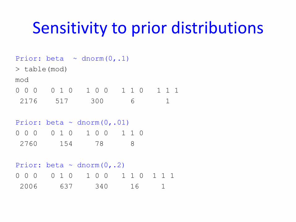
Sensitivity to prior distributions
Prior: beta ~ dnorm(0,.1)
> table(mod)
mod
0 0 0 0 1 0 1 0 0 1 1 0 1 1 1
2176 517 300 6 1
Prior: beta ~ dnorm(0,.01)
0 0 0 0 1 0 1 0 0 1 1 0
2760 154 78 8
Prior: beta ~ dnorm(0,.2)
0 0 0 0 1 0 1 0 0 1 1 0 1 1 1
2006 637 340 16 1
Model selection summary
Model selection based on posterior model probabilities, when models represent different fixed covariates, is easy to accomplish using variable weights.
The prior makes a difference, so be careful.
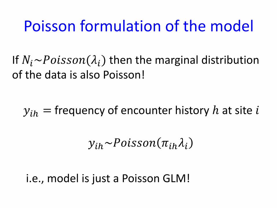
Poisson formulation of the model
If 𝑁𝑖~𝑃𝑜𝑖𝑠𝑠𝑜𝑛(𝜆𝑖) then the marginal distribution of the data is also Poisson!
𝑦𝑖ℎ = frequency of encounter history ℎ at site 𝑖
𝑦𝑖ℎ~𝑃𝑜𝑖𝑠𝑠𝑜𝑛 𝜋𝑖ℎ𝜆𝑖
i.e., model is just a Poisson GLM!
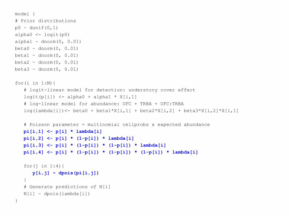
model {
# Prior distributions
p0 ~ dunif(0,1)
alpha0 <- logit(p0)
alpha1 ~ dnorm(0, 0.01)
beta0 ~ dnorm(0, 0.01)
beta1 ~ dnorm(0, 0.01)
beta2 ~ dnorm(0, 0.01)
beta3 ~ dnorm(0, 0.01)
for(i in 1:M){
# logit-linear model for detection: understory cover effect
logit(p[i]) <- alpha0 + alpha1 * X[i,1]
# log-linear model for abundance: UFC + TRBA + UFC:TRBA
log(lambda[i])<- beta0 + beta1*X[i,1] + beta2*X[i,2] + beta3*X[i,2]*X[i,1]
# Poisson parameter = multinomial cellprobs x expected abundance
pi[i,1] <- p[i] * lambda[i]
pi[i,2] <- p[i] * (1-p[i]) * lambda[i]
pi[i,3] <- p[i] * (1-p[i]) * (1-p[i]) * lambda[i]
pi[i,4] <- p[i] * (1-p[i]) * (1-p[i]) * (1-p[i]) * lambda[i]
for(j in 1:4){
y[i,j] ~ dpois(pi[i,j])
}
# Generate predictions of N[i]
N[i] ~ dpois(lambda[i])
}
Poisson model with random effects
• [see R script]
Data Augmentation (DA) Motivation
• ovenbird, ALFL, MHB data are all classical “capture-recapture” data/models but for those we formulated the model in terms of encounter frequencies for each site (a multinomial vector that is site specific). We modeled the latent 𝑁𝑖 variables as Poisson (or NB, etc..)
• In those models there is no INDIVIDUAL IDENTITY (only a site identity)
• DA gives us an alternative formulation of the model that preserves individual identity so that we may model individual effects in addition to site effects
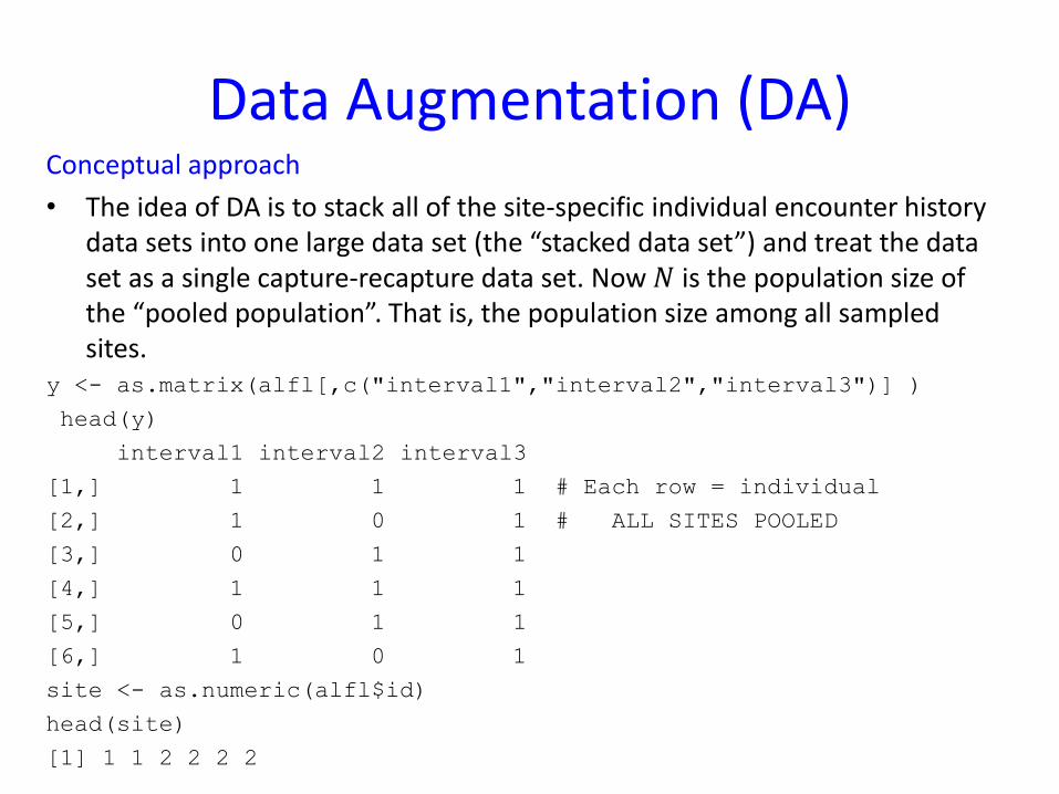
Data Augmentation (DA) Conceptual approach
• The idea of DA is to stack all of the site-specific individual encounter history data sets into one large data set (the “stacked data set”) and treat the data set as a single capture-recapture data set. Now 𝑁 is the population size of the “pooled population”. That is, the population size among all sampled sites.
y <- as.matrix(alfl[,c("interval1","interval2","interval3")] )
head(y)
interval1 interval2 interval3
[1,] 1 1 1 # Each row = individual
[2,] 1 0 1 # ALL SITES POOLED
[3,] 0 1 1
[4,] 1 1 1
[5,] 0 1 1
[6,] 1 0 1
site <- as.numeric(alfl$id)
head(site)
[1] 1 1 2 2 2 2

Data Augmentation (DA)
Conceptual approach
• What is the model for the “stacked” data set?
• Main technical challenge: 𝑁 is unknown! DA is meant primarily to deal with the unknown 𝑁 problem.
• First we switch topics and talk about analyzing “basic” capture-recapture models using DA to make the core methodological idea clear.
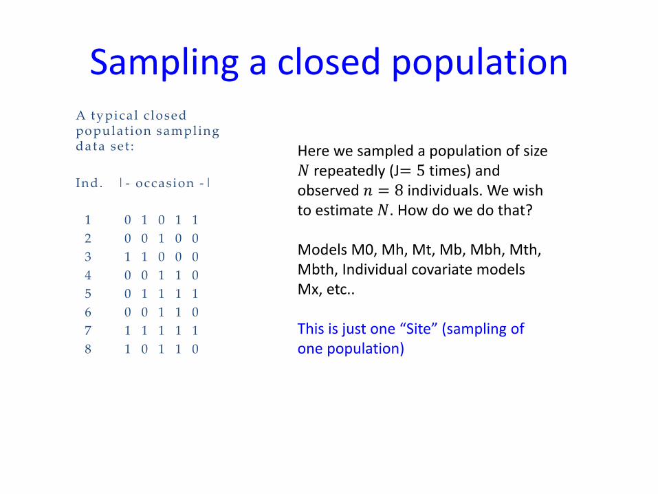
Sampling a closed population A typica l c losed populat ion sampling data set :
Ind. | - occasion -|
1 0 1 0 1 1
2 0 0 1 0 0
3 1 1 0 0 0
4 0 0 1 1 0
5 0 1 1 1 1
6 0 0 1 1 0
7 1 1 1 1 1
8 1 0 1 1 0
Here we sampled a population of size 𝑁 repeatedly (J= 5 times) and observed 𝑛 = 8 individuals. We wish to estimate 𝑁. How do we do that? Models M0, Mh, Mt, Mb, Mbh, Mth, Mbth, Individual covariate models Mx, etc.. This is just one “Site” (sampling of one population)
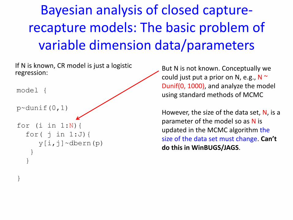
If N is known, CR model is just a logistic regression:
model {
p~dunif(0,1)
for (i in 1:N){
for( j in 1:J){
y[i,j]~dbern(p)
}
}
}
Bayesian analysis of closed capture-recapture models: The basic problem of
variable dimension data/parameters But N is not known. Conceptually we could just put a prior on N, e.g., N ~ Dunif(0, 1000), and analyze the model using standard methods of MCMC However, the size of the data set, N, is a parameter of the model so as N is updated in the MCMC algorithm the size of the data set must change. Can’t do this in WinBUGS/JAGS.

• Prior distributions: – N ~ Dunif(0, M), for M some big number (Fixed)
– p ~ uniform(0,1)
• Not amenable to a naïve implementation by MCMC (esp in BUGs/JAGS) because N, a parameter, which is the size of the data set, which has to be fixed! Also “variable dimension parameter space”
– Therefore:
• RJMCM/”Trans-dimensional” Gibbs sampling • Data augmentation <- easier, can be done in BUGS
Bayesian analysis of closed population models
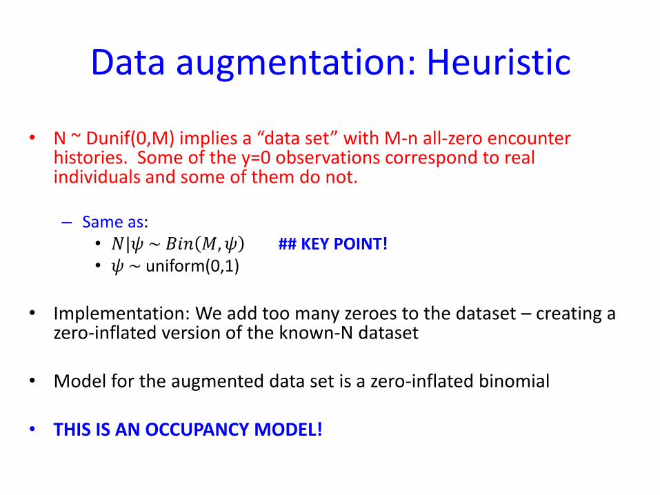
• N ~ Dunif(0,M) implies a “data set” with M-n all-zero encounter histories. Some of the y=0 observations correspond to real individuals and some of them do not.
– Same as:
• 𝑁|𝜓 ~ 𝐵𝑖𝑛 𝑀, 𝜓 ## KEY POINT! • 𝜓 ~ uniform(0,1)
• Implementation: We add too many zeroes to the dataset – creating a
zero-inflated version of the known-N dataset
• Model for the augmented data set is a zero-inflated binomial
• THIS IS AN OCCUPANCY MODEL!
Data augmentation: Heuristic
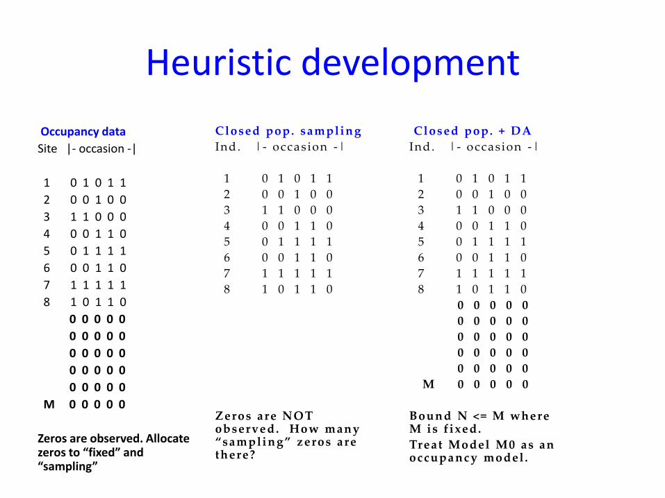
Occupancy data
Site |- occasion -|
1 0 1 0 1 1
2 0 0 1 0 0
3 1 1 0 0 0
4 0 0 1 1 0
5 0 1 1 1 1
6 0 0 1 1 0
7 1 1 1 1 1
8 1 0 1 1 0
0 0 0 0 0
0 0 0 0 0
0 0 0 0 0
0 0 0 0 0
0 0 0 0 0
M 0 0 0 0 0
Zeros are observed. Allocate zeros to “fixed” and “sampling”
Heuristic development
Closed pop. sampling
Ind. | - occas ion -|
1 0 1 0 1 1
2 0 0 1 0 0
3 1 1 0 0 0
4 0 0 1 1 0
5 0 1 1 1 1
6 0 0 1 1 0
7 1 1 1 1 1
8 1 0 1 1 0
Zeros are NOT observed. How many “sampling” zeros are there?
Closed pop. + DA
Ind. | - occas ion -|
1 0 1 0 1 1
2 0 0 1 0 0
3 1 1 0 0 0
4 0 0 1 1 0
5 0 1 1 1 1
6 0 0 1 1 0
7 1 1 1 1 1
8 1 0 1 1 0
0 0 0 0 0
0 0 0 0 0
0 0 0 0 0
0 0 0 0 0
0 0 0 0 0
M 0 0 0 0 0
Bound N <= M where M is f ixed.
Treat Model M0 as an occupancy model .
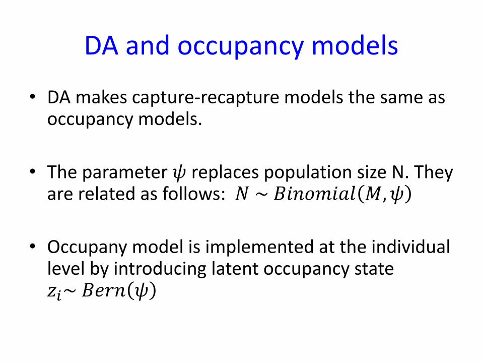
• DA makes capture-recapture models the same as occupancy models.
• The parameter 𝜓 replaces population size N. They are related as follows: 𝑁 ~ 𝐵𝑖𝑛𝑜𝑚𝑖𝑎𝑙 𝑀, 𝜓
• Occupany model is implemented at the individual level by introducing latent occupancy state 𝑧𝑖~ 𝐵𝑒𝑟𝑛 𝜓
DA and occupancy models
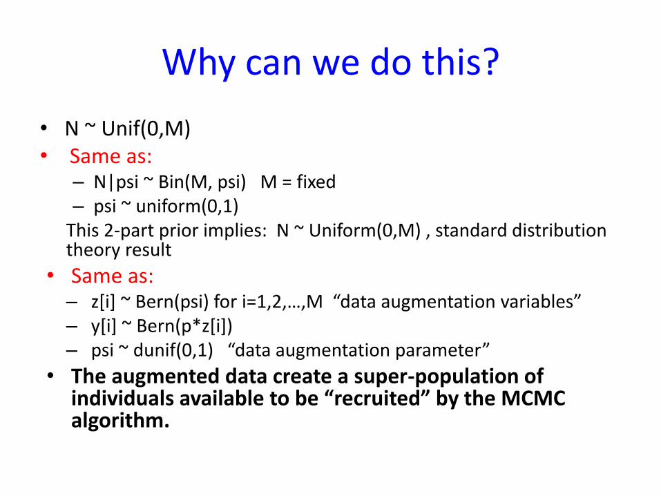
• N ~ Unif(0,M) • Same as:
– N|psi ~ Bin(M, psi) M = fixed – psi ~ uniform(0,1)
This 2-part prior implies: N ~ Uniform(0,M) , standard distribution theory result
• Same as: – z[i] ~ Bern(psi) for i=1,2,…,M “data augmentation variables” – y[i] ~ Bern(p*z[i]) – psi ~ dunif(0,1) “data augmentation parameter”
• The augmented data create a super-population of individuals available to be “recruited” by the MCMC algorithm.
Why can we do this?
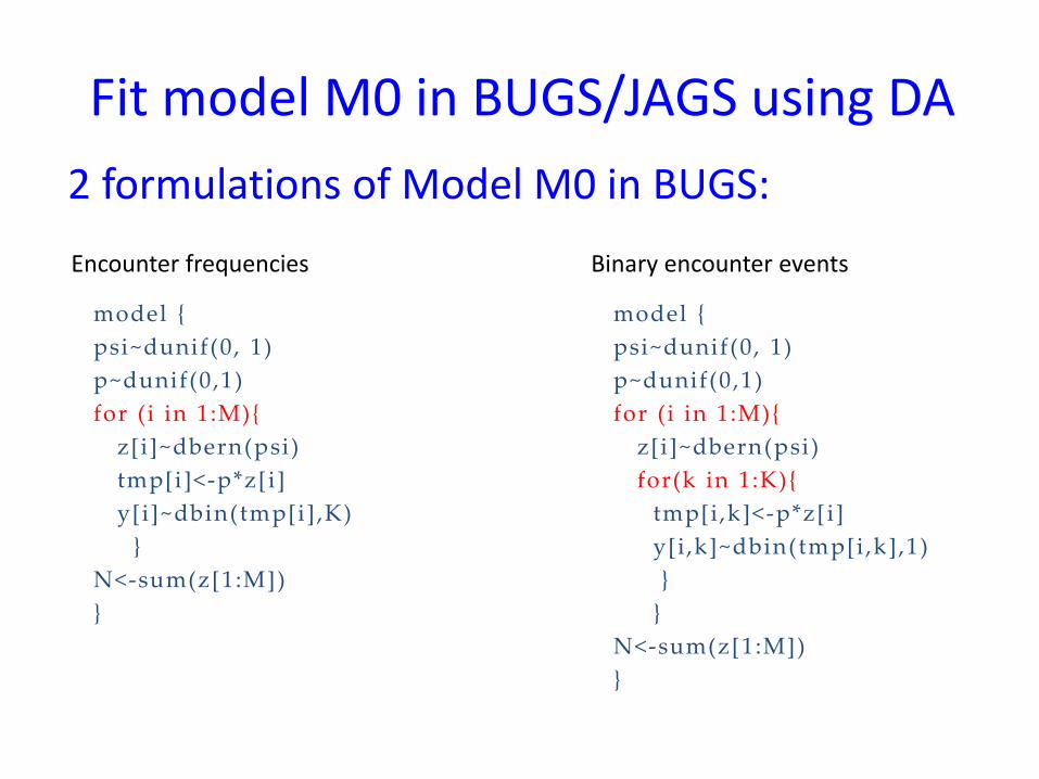
2 formulations of Model M0 in BUGS:
Fit model M0 in BUGS/JAGS using DA
model {
psi~dunif(0, 1)
p~dunif(0,1)
for (i in 1:M){
z[i]~dbern(psi)
tmp[i]<-p*z[i]
y[i]~dbin(tmp[i] ,K)
}
N<-sum(z[1:M])
}
model {
psi~dunif(0, 1)
p~dunif(0,1)
for (i in 1:M){
z[i]~dbern(psi)
for(k in 1:K){
tmp[i,k]<-p*z[i]
y[i ,k]~dbin(tmp[i ,k],1)
}
}
N<-sum(z[1:M])
}
Encounter frequencies Binary encounter events
Data Augmentation (DA)
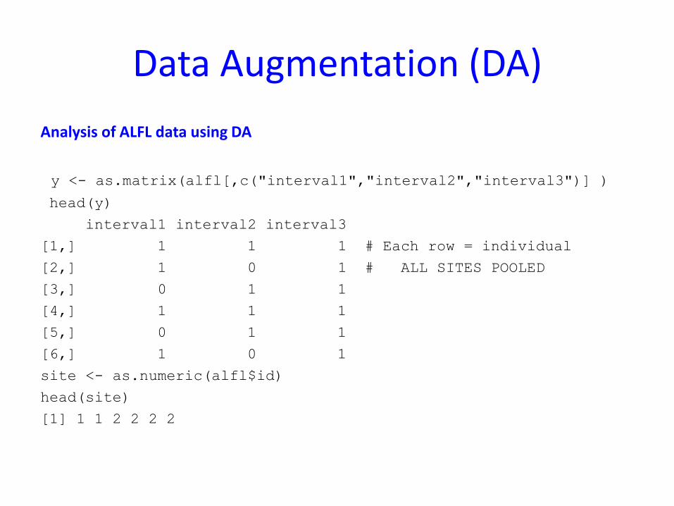
Analysis of ALFL data using DA
y <- as.matrix(alfl[,c("interval1","interval2","interval3")] )
head(y)
interval1 interval2 interval3
[1,] 1 1 1 # Each row = individual
[2,] 1 0 1 # ALL SITES POOLED
[3,] 0 1 1
[4,] 1 1 1
[5,] 0 1 1
[6,] 1 0 1
site <- as.numeric(alfl$id)
head(site)
[1] 1 1 2 2 2 2

Work session
• Analysis of the ALFL data by data augmentation
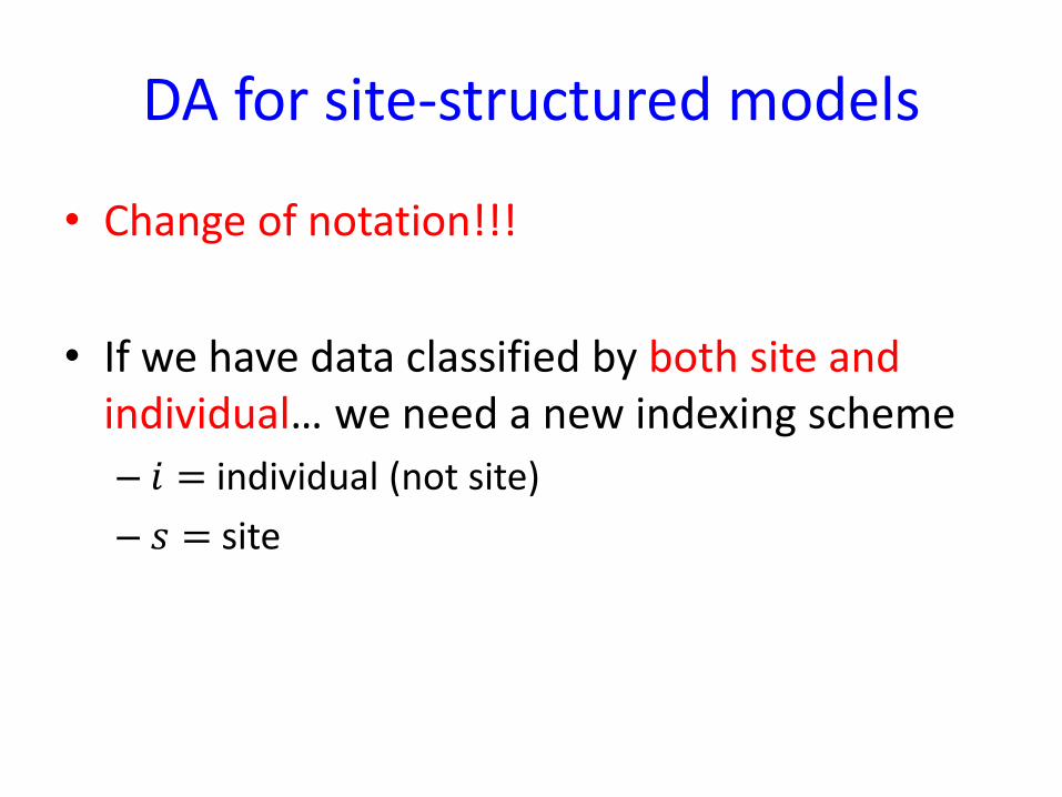
DA for site-structured models
• Change of notation!!!
• If we have data classified by both site and individual… we need a new indexing scheme
– 𝑖 = individual (not site)
– 𝑠 = site
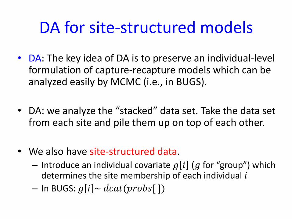
DA for site-structured models
• DA: The key idea of DA is to preserve an individual-level formulation of capture-recapture models which can be analyzed easily by MCMC (i.e., in BUGS).
• DA: we analyze the “stacked” data set. Take the data set from each site and pile them up on top of each other.
• We also have site-structured data. – Introduce an individual covariate 𝑔 𝑖 (𝑔 for “group”) which
determines the site membership of each individual 𝑖
– In BUGS: 𝑔 𝑖 ~ 𝑑𝑐𝑎𝑡(𝑝𝑟𝑜𝑏𝑠[ ])
DA for site-structured models
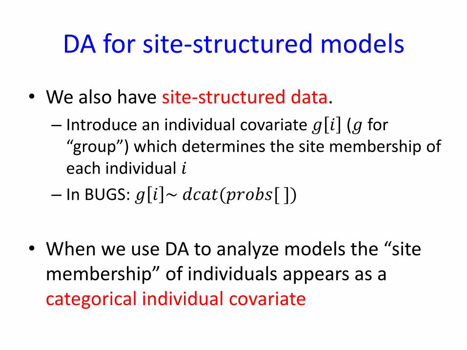
• We also have site-structured data.
– Introduce an individual covariate 𝑔 𝑖 (𝑔 for “group”) which determines the site membership of each individual 𝑖
– In BUGS: 𝑔 𝑖 ~ 𝑑𝑐𝑎𝑡(𝑝𝑟𝑜𝑏𝑠[ ])
• When we use DA to analyze models the “site membership” of individuals appears as a categorical individual covariate

DA for site-structured models
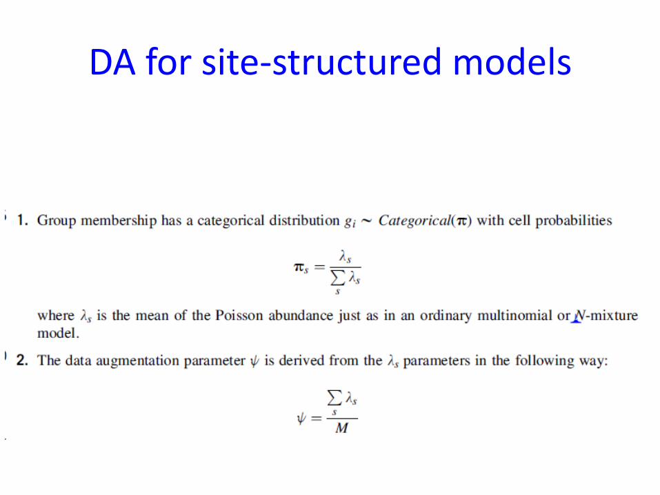
• Individual 𝑠𝑖𝑡𝑒 𝑐𝑜𝑣𝑎𝑟𝑖𝑎𝑡𝑒: 𝑔 𝑖 ~ 𝑑𝑐𝑎𝑡(𝑝𝑟𝑜𝑏𝑠[ ])
• What is 𝑝𝑟𝑜𝑏𝑠[] ????
• Derives from the assumption for 𝑁𝑠
DA for site-structured models

The end