basics of spreadsheet - national institute of open schooling 6.pdf · basics of spreadsheet ......

106 :: Data Entry Operations

Basics of Spreadsheet

6.1 INTRODUCTION

A spreadsheet is a large sheet having data and information

arranged in rows and columns. As you know, Excel is one of the

most widely used spreadsheet applications. It is a part of

Microsoft Office suite. Spreadsheet is quite useful in entering,

editing, analysing and storing data. Arithmatic operations with

numerical data such as addition, subtraction, multiplication and

division can be done using Excel. You can sort numbers/

characters according to some given criteria (like ascending,

descending etc.) and use simple financial, mathematical and

statistical formulas.

6.2 OBJECTIVES

After going through this lesson you would be able to:

l explain the basic features of MS Excel 2007

l set up pages and their printing

l modify a worksheet

l enter and edit data in a worksheet

l work on keyboard shortcuts

6

Basics of Spreadsheet :: 107

6.3 FEATURES OF SPREADSHEETS

There are a number of features that are available in Excel to

make your task easier. Some of the main features are:

1. AutoSum - helps you to add the contents of a cluster ofadjacent cells.

2. List AutoFill - automatically extends cell formatting whena new item is added to the end of a list.

3. AutoFill - allows you to quickly fill cells with repetitive orsequential data such as chronological dates or numbers,and repeated text. AutoFill can also be used to copyfunctions. You can also alter text and numbers with thisfeature.

4. AutoShapes toolbar will allow you to draw a number ofgeometrical shapes, arrows, flowchart elements, stars andmore. With these shapes you can draw your own graphs.

5. Wizard - guides you to work effectively while you work bydisplaying various helpful tips and techniques based onwhat you are doing.

6. Drag and Drop - it will help you to reposition the data andtext by simply dragging the data with the help of mouse.

7. Charts - it will help you in presenting a graphicalrepresentation of your data in the form of Pie, Bar, Linecharts and more.

8. PivotTable - it flips and sums data in seconds and allowsyou to perform data analysis and generating reports likeperiodic financial statements, statistical reports, etc. Youcan also analyse complex data relationships graphically.

9. Shortcut Menus - the commands that are appropriate tothe task that you are doing will appear by clicking the right

mouse button.

6.4 FEATURES OF MS EXCEL 2007

(a) Results-oriented user interface

The new results-oriented user interface makes it easy for you to

work in Microsoft Office Excel. Commands and features that were

often buried in complex menus and toolbars are now easier to

find on task-oriented tabs that contain logical groups ofcommands and features. Many dialog boxes are replaced with


drop-down galleries that display the available options, and

descriptive tooltips or sample previews are provided to help you

choose the right option.

(b) More rows and columns, and other new limits

The grid of Excel 2007 is having 1,048,576 rows and 16,384

columns. Thus it provides a user with 1,500% more rows and

6,300% more columns than the Microsoft Office Excel 2003. The

last column in Excel 2007, is XFD instead of IV in Excel 2003. The

number of cell references per cell is increased to limit as

maximum available memory. The formatting types are also

increased to unlimited number in the same workbook as

compared to the earlier limit of four thousand types of formatting.

(c) Office themes and Excel styles

By the help of a specific style, in Excel 2007, the data can be

quickly formatted in the worksheet by the help of a theme. You

can share themes across other releases of Office 2007 e.g. Word

2007, Power point 2007.

Applying a theme: Themes are used to make great-looking

documents. A theme is defined as a predefined set of colors,

lines, fonts and fills effects. Theme can be applied to a specific

item like tables, charts or it can also be applied to entire

workbook.

Using styles: A predefined theme based format is called style.

It can be applied to change the appearance of Excel charts, tables,

PivotTables, diagrams or shapes. Styles can be customized to

meet user specific requirements. It is important to note that in

case of charts you cannot create your own styles, but you can use

preexisting styles.

(d) Rich conditional formatting

It is easy to use and apply conditional formats. A few tricks are

required to observe the relationships in data, which helps to great

extent for analysis purposes.

Important data trends and exceptions can be easily observed by

the help of implementation and management of multiple


conditional formatting rules which apply rich visual formatting in

the form of data bars, gradient colors, and icon sets to data that

meets those rules.

(e) Easy formula writing

Some improvements that make formula writing much easier are

as given below

Resizable formula bar: To prevent the formulas to cover the other

data in worksheet, the formula bar automatically resizes to

accommodate complex, long formulas. More levels of nesting can

be used to write longer formulas as an enhanced feature of earlier

versions of Excel.

Function AutoComplete: Function AutoComplete feature helps

to write the proper formula syntax more quickly. It helps in

detecting the functions that you want to use and helps in

completing the formula.

Structured references: Excel 2007 provides structured

references to refer the named ranges and tables in a formula. This

is in addition to the cell references, like D1 and A1C1.

Easy access to named ranges: You can organize, update and

handle multiple named ranges in a central location by the help

of Excel 2007. This helps you to work on your worksheet,

interpret its data and formulas.

(f) Improved sorting and filtering

Enhanced filtering and sorting techniques of Excel can be used

to arrange worksheet data more quickly to find the desired

answers. In Excel 2007 you can sort data by color and by more

than 3 levels.

You can also filter data by color or by dates, display more than

1000 items in the AutoFilter drop-down list, select multiple items

to filter, and filter data in PivotTables.


Microsoft

Excel 2007

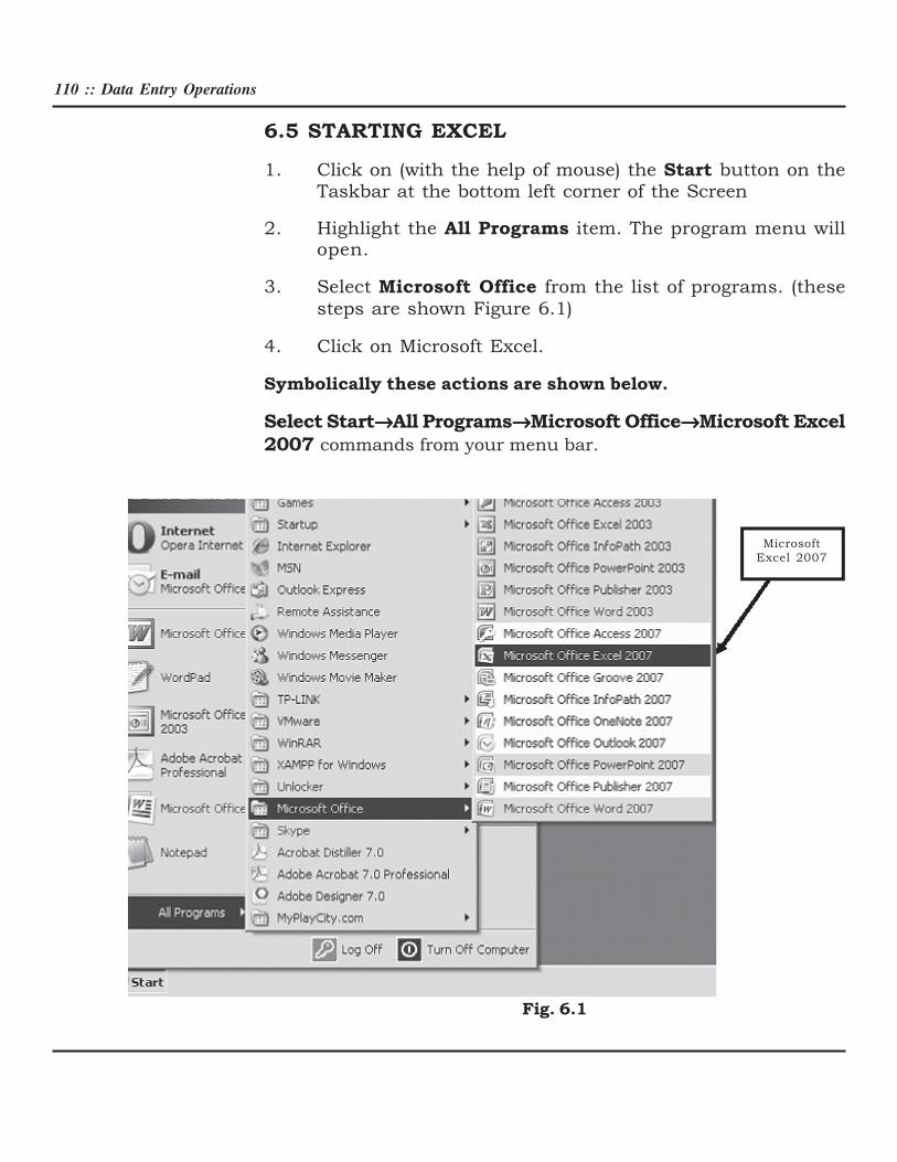
6.5 STARTING EXCEL

1. Click on (with the help of mouse) the Start button on theTaskbar at the bottom left corner of the Screen

2. Highlight the All Programs item. The program menu willopen.

3. Select Microsoft Office from the list of programs. (these

steps are shown Figure 6.1)

4. Click on Microsoft Excel.

Symbolically these actions are shown below.

Select Start→→→→→All Programs→→→→→Microsoft Office→→→→→Microsoft Excel

2007 commands from your menu bar.

Fig. 6.1


Throughout the text of your lessons on MS Excel we will be

showing the symbol→to indicate the direction (steps) you have

to follow.

You can also start Excel 2007 through run menu as shown below

in figure 6.2.

Fig. 6.2

Type excel in the open text box and click OK button. It will start

MS Excel 2007.


6.6 EXCEL WORKSHEET

Excel allows you to create worksheets much like paper ledgers

that can perform automatic calculations. Each Excel file is a

workbook that can hold many worksheets. The worksheet is a

grid of columns (designated by letters) and rows (designated by

numbers). The letters and numbers of the columns and rows

(called labels) are displayed in gray buttons across the top and

left side of the worksheet. The intersection of a column and a row

is called a cell. Each cell on the spreadsheet has a cell address

that is the column letter and the row number. Cells can contain

text, numbers, or mathematical formulas.

Fig. 6.3


6.6.1 Selecting, Adding and Renaming Worksheets

The worksheets in a workbook are accessible by clicking the

worksheet tabs just above the status bar. By default, three

worksheets are included in each workbook. One can add more

worksheet in a workbook also. To do that

Insert a new worksheet

To quickly insert a new worksheet at the end of existing

worksheets

Click the Insert Worksheet tab as shown below (encircled with

blue circle)

Fig. 6.4

To insert a new worksheet before an existing worksheet,

Select the worksheet before which you want to insert a new

worksheet then follow steps as

1. Select Home tab

2. Click cells Group

3. Click Insert

4. Click Insert Sheet

Say if you want to insert a new worksheet before a sheet name

Physics

New Worksheet


Fig. 6.5


A new sheet by the name sheet1 is added before the work sheet

named Physics.

Alternative Method to Insert a new worksheet

Right click on the sheet before which you want to insert a new

sheet

Select Insert Option from Pop up Menu

Fig. 6.6


To rename a worksheet

1. To rename a worksheet follow the steps as

2. Right click on the worksheet tab which you want to rename

3. Select rename from the Pop Up menu

4. Type new name for the Worksheet (Chemistry in our

example)

Fig. 6.7


6.7 SELECTING CELLS AND RANGES

To enter data into your worksheet you must first have a cell or

range selected. When you open an Excel worksheet, cell A1 is

already active. An active cell will appear to have a darker border

around it than other cells on the worksheet. The simplest way to

select a cell is with your mouse pointer. Move your mouse to the

desired cell and click on it with right button. Whatever you type

goes into the cell. To select a range of cells, click on one cell, hold

down the left mouse button and drag the mouse pointer to the

last cell of the range you want to select. You can also use keyboard

shortcuts given at the end of this lesson for selecting cells.

Another way to select particular range of cells is

1. Go to Name Box

2. Select range by typing (A1:C5)

3. Press Enter

4. All the cells between range A1 to C5 will be selected.

Steps are explained pictorially as


Fig. 6.8

6.8 NAVIGATING THE WORKSHEET

You can advance through your worksheet by rows with the

vertical scrollbar or by columns with the horizontal scrollbar.

When you click and drag the thumb tab on the scrollbar, a Screen

Tip will appear alongside the bar identifying the row or column

to which your view is advancing.


Move or scroll through a worksheet

We can scroll through worksheet by different ways. One can usemouse, scroll bar or arrow keys to move between cells and todifferent areas of the worksheet.

To move between cells on a worksheet, click any cell or use thearrow keys. When you move to a cell, it becomes the active cell.

Scroll and zoom by using the mouse

Some mouse devices and other pointing devices, such as theMicrosoft IntelliMouse pointing device, have built-in scrolling andzooming capabilities that you can use to move around and zoomin or out on your worksheet or chart sheet (chart sheet: A sheetin a workbook that contains only a chart. A chart sheet isbeneficial when you want to view a chart or a PivotChart reportseparately from worksheet data or a PivotTable report.). You canalso use the mouse to scroll in dialog boxes that have drop-downlists with scroll bars.

6.9 DATA ENTRY

You can enter various kinds of data in a cell.

1. Numbers: Your numbers can be from the entire range ofnumeric values: whole numbers (example, 25), decimals(example, 25.67) and scientific notation (example,0.2567E+2). Excel displays scientific notation automaticallyif you enter a number that is too long to be viewed in itsentirety in a cell. You may also see number signs (# # # # ##) when a cell entry is too long. Widening the column thatcontains the cell with the above signs will allow you to readthe number.

2. Text: First select the cell in which data has to be enteredand type the text. Press ENTER key to finish your text entry.The text will be displayed in the active cell as well as in theFormula bar. If you have numbers to be treated as text usean apostrophe (‘) as the first character. You cannot docalculations with these kind of data entry.

3. Date and Time: When you enter dates and times, Excelconverts these entries into serial numbers and kept asbackground information. However, the dates and times willbe displayed to you on the worksheet in a format opted byyou.


4. Data in Series: You can fill a range of cells either with the

same value or with a series of values with the help of

AutoFill.

6.10 EDITING DATA

Editing your Excel worksheet data is very easy. You can edit your

data by any of the following ways:

1. Select the cell containing data to be edited. Press F2. Use

Backspace key and erase the wrong entry. Retype the

correct entry.

2. Select the cell and simply retype the correct entry.

3. If you want only to clear the contents of the cell, select the

cell and press Delete key.

4. To bring back the previous entry, either click on Undo

button on standard Toolbar or select Edit→→→→→Undo command

or use keyboard shortcuts CTRL+Z.

6.11 CELL REFERENCES

Each worksheet contains a number of columns and rows. Each

cell of the worksheet has a unique reference. For example, A8,

refers to the cell containing column number A and row number 8.

6.12 FIND AND REPLACE DATA IN A WORKSHEET

You may want to locate a number or text that is already typed in

the worksheet. This is done through Home Tab→→→→→Find. You can

also locate your data and replace with new data with Home

Tab→→→→→Find→→→→→Replace.

Fig. 6.9


6.13 MODIFYING A WORKSHEET

6.13.1 Insert Cells, Rows, Columns and Delete Cells

Insert blank cells on a worksheet

l Select the cell or the range (range: Two or more cells on a

sheet. The cells in a range can be adjacent or nonadjacent.)

of cells where you want to insert the new blank cells. Select

the same number of cells as you want to insert. For

example, to insert five blank cells, you need to select five

cells.

l On the Home tab, in the Cells group, click the arrow next

to Insert, and then click Insert Cells.

l You can also right-click the selected cells and

then click Insert on the shortcut menu.

l In the Insert dialog box, click the direction in

which you want to shift the surrounding cells.

Insert rows on a worksheet

1. Do one of the following:

l To insert a single row, select the row or a cell in the

row above which you want to insert the new row. For

example, to insert a new row above row 5, click a cell

in row 5.

l To insert multiple rows, select the rows above which

you want to insert rows. Select the same number of

rows as you want to insert. For example, to insert

three new rows, you need to select three rows.

l To insert nonadjacent rows, hold down

CTRL while you select nonadjacent rows.

2. On the Home tab, in the Cells group, click the

arrow next to Insert, and then click Insert

Sheet Rows.

Insert columns on a worksheet


l To insert a single column, select the column or a cell

in the column immediately to the right of where you


want to insert the new column. For example, to insert

a new column to the left of column B, click a cell in

column B.

l To insert multiple columns, select the columns

immediately to the right of where you want to insert

columns. Select the same number of columns as you

want to insert. For example, to insert three new

columns, you need to select three columns.

l To insert nonadjacent columns, hold down CTRL

while you select nonadjacent columns.

2. On the Home tab, in the Cells group, click the

arrow next to Insert, and then click Insert

Sheet Columns.

Delete cells, rows, or columns

1. Select the cells, rows, or columns that you want to delete.

2. On the Home tab, in the Cells group, do one of the following:

l To delete selected cells, click the arrow

next to Delete, and then click Delete

Cells.

l To delete selected rows, click the arrow

next to Delete, and then click Delete

Sheet Rows.

l To delete selected columns, click the arrow next to

Delete, and then click Delete Sheet Columns.

3. If you are deleting a cell or a range of cells, in the Delete

dialog box, click Shift cells left, Shift cells up, Entire row,

or Entire column.

6.13.2 Resizing Rows and Columns

Set a column to a specific width

1. Select the column or columns that you want to

change.

2. On the Home tab, in the Cells group, click

Format.


3. Under Cell Size, click Column Width.

4. In the Column width box, type the value that you want.

Change the column width to fit the contents

1. Select the column or columns that you want to change.


Format.

3. Under Cell Size, click AutoFit Column Width.

To quickly autofit all columns on the worksheet,

click the Select All button and then double-

click any boundary between two column

headings.

Match the column width to another column

1. Select a cell in the column.

2. On the Home tab, in the Clipboard group, click

Copy, and then select the target column.


the arrow below Paste, and then click Paste

Special.

4. Under Paste, select Column widths.

Change the width of columns by using the mouse

Do one of the following:

l To change the width of one column, drag the boundary on

the right side of the column heading until the column width

changes to the desiredsize that you want.

l To change the width of multiple columns, select the

columns that you want to change, and then drag a

boundary to the right of a selected column heading.

l To change the width of columns to fit the

contents, select the column or columns

that you want to change, and then double-

click the boundary to the right of a selected

column heading.


l To change the width of all columns on the worksheet, click

the Select All button, and then drag the boundary of any

column heading.

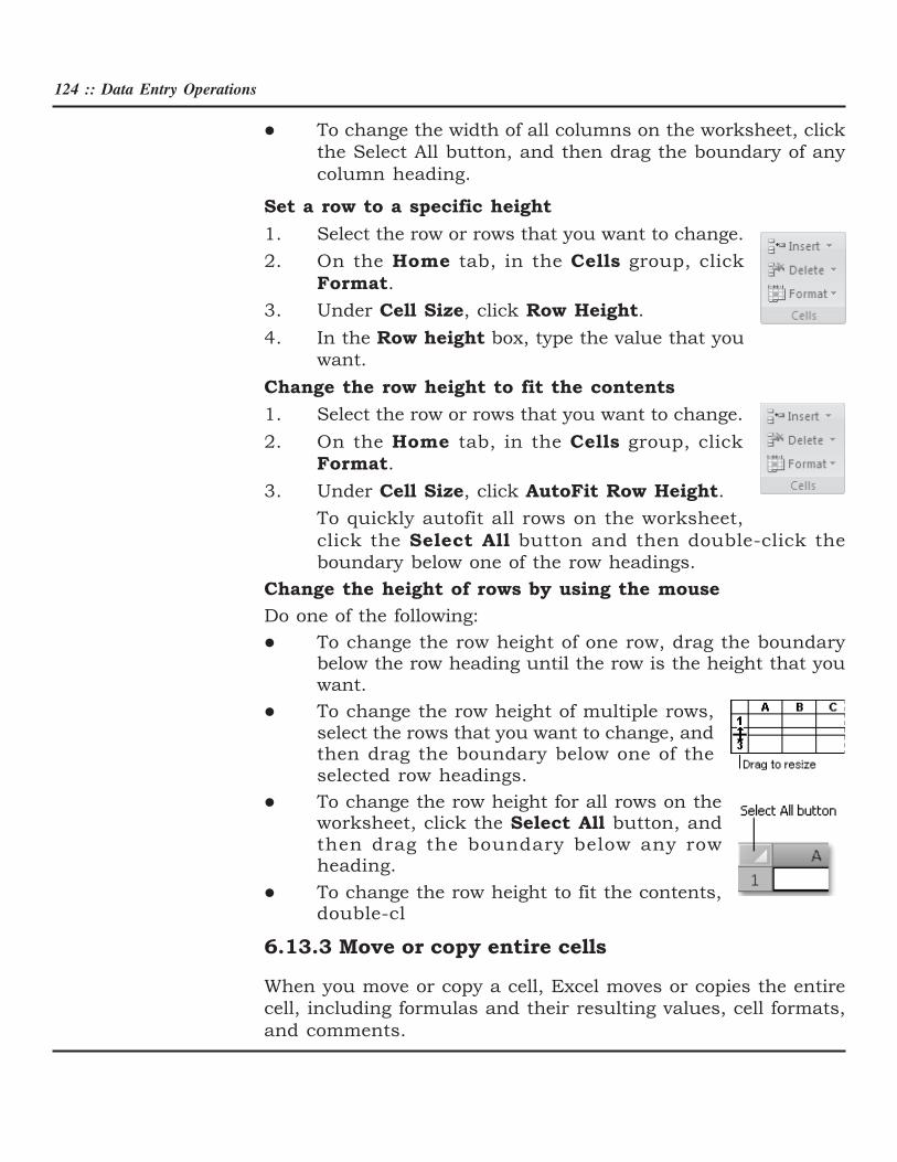
Set a row to a specific height

1. Select the row or rows that you want to change.


Format.

3. Under Cell Size, click Row Height.

4. In the Row height box, type the value that you

want.

Change the row height to fit the contents

1. Select the row or rows that you want to change.


Format.

3. Under Cell Size, click AutoFit Row Height.

To quickly autofit all rows on the worksheet,

click the Select All button and then double-click the

boundary below one of the row headings.

Change the height of rows by using the mouse

Do one of the following:

l To change the row height of one row, drag the boundarybelow the row heading until the row is the height that youwant.

l To change the row height of multiple rows,select the rows that you want to change, andthen drag the boundary below one of theselected row headings.

l To change the row height for all rows on theworksheet, click the Select All button, andthen drag the boundary below any rowheading.

l To change the row height to fit the contents,double-cl

6.13.3 Move or copy entire cells

When you move or copy a cell, Excel moves or copies the entire

cell, including formulas and their resulting values, cell formats,

and comments.


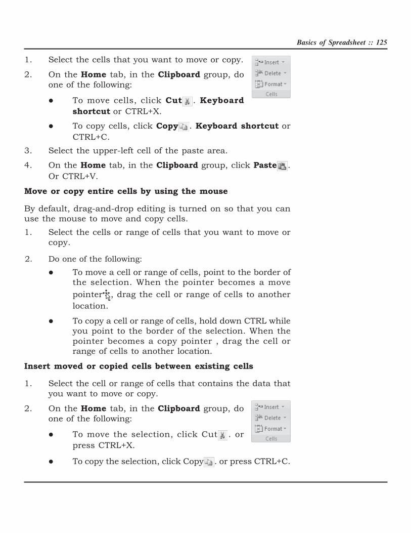
1. Select the cells that you want to move or copy.

2. On the Home tab, in the Clipboard group, do

one of the following:

l To move cells, click Cut . Keyboard

shortcut or CTRL+X.

l To copy cells, click Copy . Keyboard shortcut or

CTRL+C.

3. Select the upper-left cell of the paste area.

4. On the Home tab, in the Clipboard group, click Paste .

Or CTRL+V.

Move or copy entire cells by using the mouse

By default, drag-and-drop editing is turned on so that you can

use the mouse to move and copy cells.

1. Select the cells or range of cells that you want to move or

copy.


l To move a cell or range of cells, point to the border of

the selection. When the pointer becomes a move

pointer , drag the cell or range of cells to another

location.

l To copy a cell or range of cells, hold down CTRL while

you point to the border of the selection. When the

pointer becomes a copy pointer , drag the cell or

range of cells to another location.

Insert moved or copied cells between existing cells

1. Select the cell or range of cells that contains the data that

you want to move or copy.

2. On the Home tab, in the Clipboard group, do

one of the following:

l To move the selection, click Cut . or

press CTRL+X.

l To copy the selection, click Copy . or press CTRL+C.


3. Right-click the upper-left cell of the paste area, and then

click Insert Cut Cells or Insert Copied Cells on the

shortcut menu.

4. In the Insert Paste dialog box, click the direction in which

you want to shift the surrounding cells.

Prevent copied blank cells from replacing data

1. Select the rangeof cells that contains blank cells.

2. On the Home tab, in the Clipboard group, click Copy .

Keyboard shortcut You can also press

CTRL+C.

3. Select the upper-left cell of the paste area.


the arrow below Paste , and then click Paste

Special.

5. Select the Skip blanks check box.

Move or copy the contents of a cell

1. Double-click the cell that contains the data that you want

to move or copy.

2. In the cell, select the characters that you want to move or

copy.

To select the Do this

contents of a cell

In the cell Double-click the cell, and then drag across the

contents of the cell that you want to select.

In the formula bar Click the cell, and then drag across the contents of the

cell that you want to select in the formula bar.

By using the keyboard Press F2 to edit the cell, use the arrow keys to position

the insertion point, and then press SHIFT+ARROW key

to select the contents.

3. On the Home tab, in the Clipboard group, do one of the

following:

l To move the selection, click Cut .

l To copy the selection, click Copy .

4. In the cell, click where you want to paste the


characters, or double-click another cell to move or copy the

data.

5. On the Home tab, in the Clipboard group, click Paste .

6. Press ENTER.

Copy cell values, cell formats, or formulas only

When you paste copied data, you can do any of the following:

l Convert any formulas in the cell to the calculated values

without overwriting the existing formatting.

l Paste only the cell formatting, such as font color or fill color

(and not the contents of the cells).

l Paste only the formulas (and not the calculated values).

1. Select the cell or range of cells that contains the values, cell

formats, or formulas that you want to copy.

2. On the Home tab, in the Clipboard group, click Copy .

3. Select the upper-left cell of the paste area or the

cell where you want to paste the value, cell

format, or formula.


the arrow below Paste , and then do one of the

following:

l To paste values only, click Paste Values.

l To paste cell formats only, click Paste Special, and then

click Formats under Paste.

l To paste formulas only, click Formulas.

Drag and Drop

If you are moving the cell contents only a short distance, the drag-

and-drop method may be easier. Simply drag the highlighted

border of the selected cell to the destination cell with the mouse.

Freeze Panes

If you have a large worksheet with column and row headings,

those headings will disappear as the worksheet is scrolled. By

using the Freeze Panes feature, the headings can be visible at

all times.


1. Click the label of the row below the row that should remain

frozen at the top of the worksheet.

2. Select View Tab→→→→→Window Group on ribbon→→→→→Freeze

Panes→→→→→Freeze Panes

3. To remove the frozen panes, View Tab→→→→→Window Group on

ribbon→→→→→Freeze Panes→→→→→Unfreeze Panes

Fig. 6.10

Freeze panes has been added to row 2 in the image above. Notice

that the row numbers skip from 1 to 11. As the worksheet is

scrolled, rows 1 will remain stationary while the remaining rows

will move. Following similar steps you can Freeze or Unfreeze

selected columns.


Fig. 6.11

Unfreeze Panes option will come only if the respective panes are

already Freeze.

6.14 PAGE BREAKS

To set page breaks within the worksheet, select the row you want

to appear just below the page break by clicking the row’s label.

Then choose Page Layout→→→→→Setup Group→→→→→Breaks→→→→→Input Page

Break. Excel will start a new page from the row selected.

Fig. 6.12


6.15 PAGE SETUP

Select File→Page Setup from the menu bar to format the page,

set margins, and add headers and footers.

1. Page: The page option allows you to set the paper size,

orientation of the data, scaling of the area, print quality, etc.

Select the Orientation under the Page tab in the Page Setup

window to make the page Landscape or Portrait. The size

of the worksheet on the page can also be formatted using

Scaling. To force a worksheet to print only one page wide

so that all the columns appear on the same page, select Fit

to 1 page(s) wide.

Fig. 6.13


2. Margins: Change the top, bottom, left, and right margins

by selecting Margins from the page setup group of age

Layout Tab. Enter values in the header and footer fields to

indicate how far from the edge of the page this text should

appear. Check the boxes for centering horizontally or

vertically on the page.

Fig. 6.14

There are three predefined margin settings. You can choose from

them or you can also customize the margins as shown by the

following diagram.

Fig. 6.15


3. Add or change the header or footer text: For worksheets,

you can work with headers and footers in Page Layout view.

For other sheet types, such as chart sheets or for embedded

charts, you can work with headers and footers in the Page

Setup dialog box.

Add or change the header or footer text for a worksheet in

Page Layout view

1. Click the worksheet to which you want to add headers or

footers, or that contains headers or footers that you want

to change.

2. On the Insert tab, in the Text

group, click Header & Footer.


l To add a header or footer, click the left, center, or right

header or footer text box at the top or at the bottom

of the worksheet page.

l To change a header or footer, click the header or

footer text box at the top or at the bottom of the

worksheet page that contains header or footer text,

and then select the text that you want to change.

4. Type the text that you want.

To close the headers or footers, click anywhere in the

worksheet, or press ESC.

5. Sheet tab has the option to select the area to be printed

(that is, range of cells). Check Gridlines if you want the

gridlines dividing the cells to be printed on the page. If the

worksheet is several pages long and only the first page

includes titles for the columns, select Rows to repeat at

top to choose a title row that will be printed at the top of

each page.


Fig. 6.16

6.16 PRINT PREVIEW

Print preview helps to view the worksheet before the final printout

is taken. It helps to edit the worksheet if required as per the need.

The steps to see the print view of document

1. Select Print from Office Button .

2. Select print

3. Click Print Preview.


Fig. 6.17

Click the buttons like Next and Previous with respect to Print

Preview Tab. Select the Zoom button to view the pages closer.

Make page layout modifications needed by clicking the Page

Setup button. Click Close to return to the worksheet or Print to

continue printing.

6.17 PRINT

To print the worksheet, select Print from Office Button .


Fig. 6.18

1. Print Range - Select either all pages or a range of pages to

print.

2. Print What - Select selection of cells highlighted on the

worksheet, the active worksheet, or all the worksheets in

the entire workbook.

3. Copies - Choose the number of copies that should be

printed. Check the Collate box if the pages should remain

in order.

4. Click OK to print.

6.18 FILE OPEN, SAVE AND CLOSE

(A) You can open an existing File by several methods:

1. Go to windows explorer and find out the file you want

to open. Double-click on the file.

2. Start MS Excel. Click on office button on the drop-

down menue click 'open'. select the file you want to

open from the pop-up menu.

(B) When you have finished your work on the file you can save

it by either clicking on the 'file save' icon at the top left


corner or Click on office button →→→→→ click on save at the drop-

down menu.

(C) When you are saving the worksheet for the first time follow

the steps given below:

1. Click office button

2. Select 'file save as'on the drop-down menu.

3. On the pop-up menu select the location where you

want to save the file.

4. Type the file name

5. Click on 'save'in the pop-up menu.

(D) When your work is finished and it has been saved properly:

Select Print from Office Button

1. Select (Click) Close Command to close your file

2. Select (Click) Exit Excel Command to exit from MS

Excel

Fig. 6.19


6.19 WORKBOOK PROTECTION

Set a password for a workbook

1. Click the Microsoft Office Button , and then click Save

As.

2. Click Tools, and then click General Options.

3. Do one or both of the following:

l If you want reviewers to enter a password before they

can view the workbook, type a password in the

Password to open box.

l If you want reviewers to enter a password before they

can save changes to the workbook, type a password

in the Password to modify box.

4. If you don’t want content reviewers to accidentally modify

the file, select the Read-only recommended check box.

When opening the file, reviewers will be asked whether or

not they want to open the file as read-only.

5. Click OK.

6. When prompted, retype your passwords to confirm them,

and then click OK.

7. Click Save.

8. If prompted, click Yes to replace the existing workbook.

INTEXT QUESTIONS

1. Write True or False for the following statements

(a) To modify a preset header or footer click the custom

header and custom footer buttons.

(b) Autofill helps you to add the contents of a cluster of

adjacent cells.

(c) Charts features help you in presenting a graphical

representation of data.

(d) Click the edit button to print the worksheet.

(e) Pivot table allows you to perform data analysis.


2. Fill in the blanks

(a) When the active document is protected the command

name changes to ________________ workbook.

(b) Select __________________ from the menu bar to view

how the worksheet will look when printed.

(c) _________ toolbar allows to draw a number of

geometrical shapes, arrows, flow chart elements etc.

(d) Check ______________ if you want the gridlines

dividing the cells to be printed on the page.

6.20 WHAT YOU HAVE LEARNT

In this lesson you learnt about starting Excel and working on a

worksheet. You can select a cell or a range of cells. Also you can

enter data in a worksheet. You can define the size of a page by

going to page set up and insert a page break. You have learnt

about page-preview which gives an idea on how the print out will

look like.

6.21 TERMINAL QUESTIONS

1. What are the main features of MS Excel?

2. Differentiate between a worksheet and a workbook?

3. What are the different types of data that can be entered into

worksheet cells?

4. Explain three different ways you protect your workbook.

5. How do you find a single number or name you want in a

large worksheet containing thousands of numbers and

names? Is it possible to replace a name or number with

some other name or number? How?

6. How do you select a single cell, a single column, a single

row, a cluster of cells, and a entire worksheet?

7. Difference between Move cells and Copy cells

8. What are the different features available in Page setting

command?


8. Explain the different features available in Print command?

10. Define the following:

(a) Navigating worksheet

(b) Editing data

(c) Insert cells and rows

(d) Drag and drop

(e) Workbook protection

6.22 FEEDBACK TO INTEXT QUESTIONS

1. (a) True (b) False (c) True (d) False (e) True

2. (a) Unprotect (b) Print preview (c) Autoshapes

(d) gridlines

basics of spreadsheet - national institute of open schooling 6.pdf · basics of spreadsheet ......

Documents