attitude toward statistic in college students (an ... 2_1_4.pdf · universidad politécnica de...

Journal of Statistical and Econometric Methods, vol. 2, no.1, 2013, 43-60

ISSN: 2051-5057 (print version), 2051-5065(online)

Scienpress Ltd, 2013

Attitude toward Statistic in College Students

(An Empirical Study in Public University)

Arturo García-Santillán1, Francisco Venegas-Martinez

2, Milka Elena Escalera

Chávez3 and Arturo Córdova-Rangel

4

Abstract

This study aims to measure student’s attitude towards statistics through a model that

considers the variables proposed by Auzmendi (1992). Was examined whether the

constructs: usefulness, motivation, likeness, confidence and anxiety influence the

student's attitude towards statistics. Were surveyed face to face 328 students at the

Universidad Politécnica de Aguascalientes using the questionnaire proposed by

Auzmendi. The statistical procedure used was factorial analysis with an extracted

principal component. The Statistics Hypothesis: Ho: ρ = 0 has no correlation, while Ha: ρ

≠ 0 does. Statistics test to prove: Χ2, Bartlett‟s test of sphericity, KMO (Kaiser-

Meyer_Olkin) Significance level: α = 0.05; p < 0.01 The results obtained from the

sphericity test of Bartlett KMO (0.592), Chi square X2 390.552 df 10, Sig. 0.00 < p 0.01,

MSA (Usefulness 0.656, Motivation 0.552, Likeness 0.705, Confidence 0.633 and

Anxiety 0.507). With all this we obtained significant evidence in order to reject Ho.

Finally we obtained two factors that explain attitude toward statistic in college students:

One of them is composed by three elements: Confidence (.852), Likeness (.818) and

Usefulness (.768) and the other is composed by two elements: Anxiety (.837) and

Motivation (.800). Their explanatory power for each factor is expressed by their

Eigenvalue: 2.170 and 1.383 (with % variance 43.39 and 27.67 respectively, Total

variance explained 71.05%).

Keywords: Components, usefulness, motivation, likeness, confidence and anxiety

1Administrative-Economic Research Center at Cristóbal Colón University (Mexico)

e-mail: [email protected] 2School of Economy at National Polytechnic Institute (IPN Mexico)

e-mail: [email protected] 3Multidisciplinary Unit Middle Zone at Autonomous University of San Luis Potosí, (SLP-México)

e-mail: [email protected] 4Business Research Center at Universidad Politécnica de Aguascalientes (Mexico)

e-mail: [email protected]

Article Info: Received : November 15, 2012. Revised : December 18, 2012.

Published online : March 1, 2013

mailto:[email protected]




44 Arturo García-Santillán et al.

1 Introduction

1.1 Attitude towards Statistic

As refers García-Santillán, Venegas-Martinez and Escalera-Chávez (2013), in the

academic institutions, the great majority of the courses offering similar services within the

undergraduate and posdegree graduate have been integrated in the curriculums, of

mathematics subjects, such as: statistics, calculus, financial engineering and more. As a

result, thousands of students in degrees and other specialties not mathematically oriented,

continue taken statistics courses worldwide, all this like say Blanco (2008). Also in

several studies have been reported: emotional reactions, attitudes and negative beliefs

from students towards statistics and with little interest in this subject and a limited

quantitative training (Blanco, 2004). It is therefore necessary to continue to explore about

this issue, in order to provide empirical evidence that may contributing to the redefinition

of the teaching strategies in the teaching-learning process in this regard.

One of the first operative definition and measure about attitude toward statistics is the test

of Roberts and Bildderbach (1980) denominated Statistics Attitudes Survey (SAS). It’s

considered the first measure about construct called “Attitude toward statistics” in fact,

was made with the intention of providing a focused test in statistics field in order to

measure this subject, from the tradition and professional work of students. In this order of

ideas, some arguments exposed in Garcia-Santillán, Venegas-Martinez and Escalera-

Chávez (2013) refers that, into the educational research, statistical level has justified the

need to pay attention to students’ attitude mainly because they have an important

influence on the process of teaching and learning and the same way, the immediate

academic performance (such as variable input and process).

In the same sense, the argument exposed by Auzmendi (1992), Gal & Ginsburg (1994)

and Ginsburg & Schau (1997) about students’ attitude toward statistic; they point out that,

the attitude is an essential component of the background of student with which, after its

university training, may carry out academic and professional activities (cited in Blanco

2008). Other research (Mondejar, Vargas and Bayot, 2008) developed a test based on the

methodological principles of Wise (1985) attitude toward statistic (ATS) and scale

attitude toward statistics (SATS) of Auzmendi (1992).

About scale ATS, is structured of 29 items grouped in two scales, one that measures the

affective relationship with learning and cognitive measures the perception of the student

with the use of statistics. Mondéjar et al (2008) refer to that initially validation was based

on a sample very small, and was with subsequent studies such as Mondejar et al (2009) or

Woehlke (1991) who´s corroborated this structure, and the work of Gil (1999) choose to

use an structure with five factors: one of the emotional factor and the remaining four

factors related cognitive component. The objectives were to develop a test on students

‘attitude statistic and his analyze on influence in the form to study. Mondéjar et al (2008)

describe the psychometric properties of this new scale to measuring attitude toward

statistics; the result obtained is the creation of a good tool to measuring or quantifying the

students´ affective factors. Besides, the result may show the level of nervousness and

anxiety and other factors: such a gender and how the course studied may affect the study

process. All this could affect students´ attitude like say Phillips (1980), he refers to, that

the students’ attitude can suppose an obstacle or constituted and advantages for their

learning.

Attitude toward Statistic in College Students 45

Meanwhile, Roberts and Saxe (1982); Beins (1985); Wise (1985); Katz and Tomezik

(1988); Vanhoof et al (2006) and Evans (2007) showed the relationship between attitude

toward statistic and academic outcomes or the professional use of this tool. They have

demonstrated the existence of positive correlation among college students’ attitudes and

their performance in this matter.

Similar are the studies in Spain performed by Auzmendi (1992), Sánchez-López (1996)

and Gil (1999) that also have demonstrated that there are a positive correlation among

attitude of college student and their performance. Important background is the work of

Wise (1985) and Auzmendi (1992) with the scales ATS y SATS, who have tried to

measure the job that underlies this issue. They obtained the most important

characteristics of the students regarding their attitude toward statistics, their difficulties

with the mathematical component and the prejudice to this issue. To this argument,

similarly, there are added the works of Elmore and Lewis (1991) and Schau et al (1995).

Finally we can say that the review of literature about this subject, Blanco (2008) it carried

out a critical review on research on students’ attitude toward statistics and describe, some

inventories test that measure specifically the students’ attitude statistic. In his study refer

the research of Cherian and Glencross (1997) who cited the most important studies in the

Anglo-Saxon context such as: Statistics Attitudes Survey- SAS Roberts & Bilderback

(1980), Roberts & Reese, (1987), Attitudes toward Statistics- ATS Wise (1985 ), Statistics

Attitude Scale McCall, Belli & Madjini (1991), Statistics Attitude Inventory (Zeidner,

1991), Students´Attitudes Toward Statistics Sutarso (1992 ), Attitude Toward Statistics

Miller, Behrens, Green and Newman (1993), Survey of Attitudes Toward Statistics –SATS

Schau, Stevens, Dauphinee and Del Vecchio (1995), Quantitative Attitudes Questionnaire

Chang (1996) among other.

With the above, and considering that we find answers to the research questions about

attitude towards statistic in engineering undergraduate students, we use the scale proposed

by Auzmendi. Thus, it set the following:

1.2 Question Research, Objective and Hypothesis

RQ1. Which the attitude toward statistic in college students?

RQ2. What factors can help explain the attitude toward statistic in college students?

Objectives

So1. Determine the level attitude toward statistic in college students.

So2. Identify which are the factors that explain attitude toward statistic in college students.

The following hypotheses were established from the previously exposed questions:

H1: Likeness is the factor that most explained the student’s attitude towards statistic

H2: Anxiety is the factor that most explained the student’s attitude towards statistic

H3: Confidence is the factor that most explained the student’s attitude towards statistic

H4: Motivation is the factor that most explained the student’s attitude towards statistic

H5: Usefulness is the factor that most explained the student’s attitude towards statistic


2 Materials and Methods

2.1 Design Methodology, Population and Sample

This study is non experimental, transeccional-descriptive, because we need to know the

attitude toward statistics in college students at Universidad Politécnica de Aguascalientes.

The sample was selected for the trial of non-probability sampling. Were surveyed face to

face 328 students at Universidad Politécnica de Aguascalientes from several profiles, as;

Engineering in Mechanical, Mecatrónic, Industrial, Strategic System of Information and

finally, Business and Management.

The selection criteria were to include students who have completed at least one field of

statistics in the degree program they were studying and were available at the institution to

implement the survey. The instrument used was a survey of attitudes toward statistics or

SATS (Auzmendi, 1992). The scale proposed by Auzmendi indicates the existence of five

factors: usefulness, anxiety, confidence, pleasure and motivation. The usefulness factor

indicators are: Item 1, 6, 11, 16, 21; anxiety factor indicators are: Item 2, 7, 12, 17, 22; the

confidence factor are: items 3, 8, 13, 18, 23; likeness factor indicators are: Item 4, 9, 14,

19, 24. Finally indicators belonging to motivational factor are: items 5, 10, 15, 20, 25. The

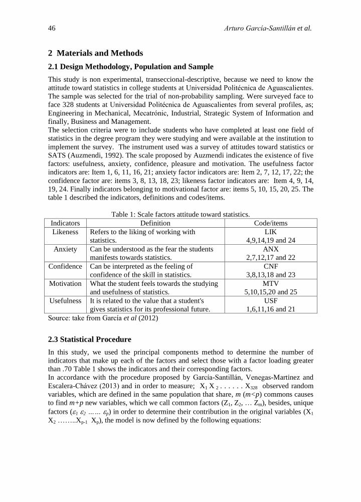
table 1 described the indicators, definitions and codes/items.

Table 1: Scale factors attitude toward statistics.

Indicators Definition Code/items

Likeness Refers to the liking of working with

statistics.

LIK

4,9,14,19 and 24

Anxiety Can be understood as the fear the students

manifests towards statistics.

ANX

2,7,12,17 and 22

Confidence Can be interpreted as the feeling of

confidence of the skill in statistics.

CNF

3,8,13,18 and 23

Motivation What the student feels towards the studying

and usefulness of statistics.

MTV

5,10,15,20 and 25

Usefulness It is related to the value that a student's

gives statistics for its professional future.

USF

1,6,11,16 and 21

Source: take from García et al (2012)

2.3 Statistical Procedure

In this study, we used the principal components method to determine the number of

indicators that make up each of the factors and select those with a factor loading greater

than .70 Table 1 shows the indicators and their corresponding factors.

In accordance with the procedure proposed by García-Santillán, Venegas-Martinez and

Escalera-Chávez (2013) and in order to measure; X1 X 2 . . . . . . X328 observed random

variables, which are defined in the same population that share, m (m<p) commons causes

to find m+p new variables, which we call common factors (Z1, Z2, … Zm), besides, unique

factors (1 2 …… p) in order to determine their contribution in the original variables (X1

X2 ……..Xp-1 Xp), the model is now defined by the following equations:


1 11 1 12 2 1m m 1 1

2 21 1 22 2 2m m 2 2

p p1 1 p2 2 pm m p p

X = a Z + a Z +..........a Z + b ξ

X = a Z + a Z +..........a Z + b ξ

.......................................................................

X = a Z + a Z +..........a Z + b ξ

(1)

Where:

Z1, Z2, … Zm are common factors

1 2 …… p are unique factors

Thus, 1 2 …… p have influence in all variables Xi ( i=1 ………p) i

ξ influence in

Xi(i=1……..p)

Model equations can be expressed in matrix form as follow:

=

.

(2)

Therefore, the resulting model can be expressed in a condensed form as:

i

X AZ ξ (3)

Where, we assume that m<p because they want to explain the variables through a small

number of new random variables and all of the (m + p) factors are correlated variables,

that is, that the variability explained by a variable factor, have not relation with the other

factors.

We know that the each observed variable of model is a result of lineal combination of

each common factor with different weights (aia), those weights are called saturations, but

one of part of xi is not explained for common factors. As we know, all problems intuitive

can be inconsistent when obtaining solutions and therefore, we require the approach of

hypothesis; hence, in the factor model we used the following assumptions:

H1: The factors are typified random variables, and inter correlated, like:

iE Z =0 i

E ξ =0 i iE Z Z =1

i iE ξ ξ =1 ,

i i

E Z Z =0 , i i

E ξ ξ =0

i iE Z ξ =0

Further, we must consider that the factors have a primary goal to study and simplify the

correlations between variables, measures, through the correlation matrix, then, we will

understand that:

H2: The original variables could be typified by transforming these variables of type -

i

i

x

x - xx =

σ (4)

Therefore, and considering the variance property we have:


2 2 2 2

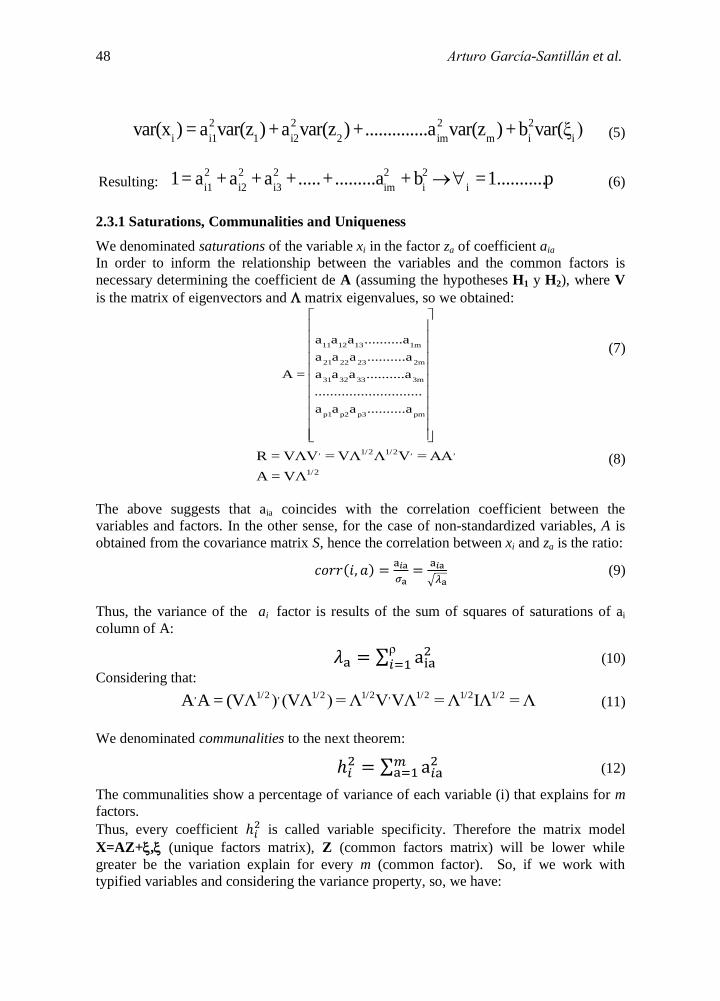
i i1 1 i2 2 im m i ivar(x ) = a var(z ) +a var(z ) +..............a var(z ) + b var(ξ ) (5)

Resulting: 2 2 2 2 2

i1 i2 i3 im i i1= a + a + a +.....+.........a + b =1...........p (6)

2.3.1 Saturations, Communalities and Uniqueness

We denominated saturations of the variable xi in the factor za of coefficient aia

In order to inform the relationship between the variables and the common factors is

necessary determining the coefficient de A (assuming the hypotheses H1 y H2), where V

is the matrix of eigenvectors and matrix eigenvalues, so we obtained:

11 12 13 1m

21 22 23 2m

31 32 33 3m

p1 p2 p3 pm

a a a ..........a

a a a ..........a

A = a a a ..........a

............................

a a a ..........a

(7)

, 1/2 1/2 , ,

1/2

R = VΛV = VΛ Λ V = AA

A = VΛ

(8)

The above suggests that aia coincides with the correlation coefficient between the

variables and factors. In the other sense, for the case of non-standardized variables, A is

obtained from the covariance matrix S, hence the correlation between xi and za is the ratio:

=

=

(9)

Thus, the variance of the ai factor is results of the sum of squares of saturations of ai

column of A:

= ρ

(10)

Considering that: , 1/2 , 1/2 1/2 , 1/2 1/2 1/2A A = (VΛ ) (VΛ ) = Λ V VΛ = Λ IΛ = Λ (11)

We denominated communalities to the next theorem:

=

(12)

The communalities show a percentage of variance of each variable (i) that explains for m

factors.

Thus, every coefficient is called variable specificity. Therefore the matrix model

X=AZ+, (unique factors matrix), Z (common factors matrix) will be lower while

greater be the variation explain for every m (common factor). So, if we work with

typified variables and considering the variance property, so, we have:


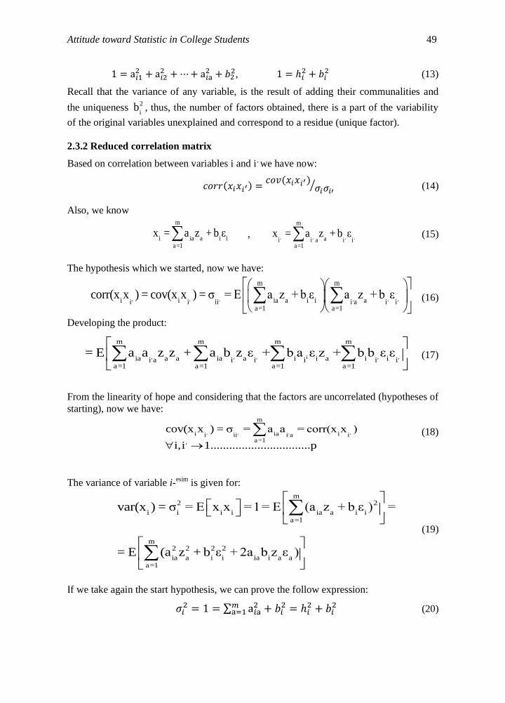
1 =

, 1 =

(13)

Recall that the variance of any variable, is the result of adding their communalities and

the uniqueness 2

ib , thus, the number of factors obtained, there is a part of the variability

of the original variables unexplained and correspond to a residue (unique factor).

2.3.2 Reduced correlation matrix

Based on correlation between variables i and i, we have now:

=

(14)

Also, we know m

i ia a i ia=1

x = a z + b ε ,

m

ai i a i ia=1

x = a z + b ε, , , , (15)

The hypothesis which we started, now we have:

, , , , , ,

m m

i i ia a i i ai i ii i a i ia=1 a=1

corr(x x ) = cov(x x ) = σ = E a z + b ε a z + b ε (16)

Developing the product:

, , , i , ,

m m m m

ia a a ia a i i a i ii a i i i i ia=1 a=1 a=1 a=1

= E a a z z + a b z ε + b a ε z + b b ε ε (17)

From the linearity of hope and considering that the factors are uncorrelated (hypotheses of

starting), now we have:

, , , ,

m

i ia ii ii i a ia=1,

cov(x x ) = σ = a a = corr(x x )

i,i 1................................p

(18)

The variance of variable i-esim is given for:

m2 2

i i i i ia a i ia=1

m2 2 2 2

ia a i i ia i a aa=1

var(x ) = σ = E x x =1= E (a z + b ε ) =

= E (a z + b ε + 2a b z ε )

(19)

If we take again the start hypothesis, we can prove the follow expression:

= 1 =

=

(20)


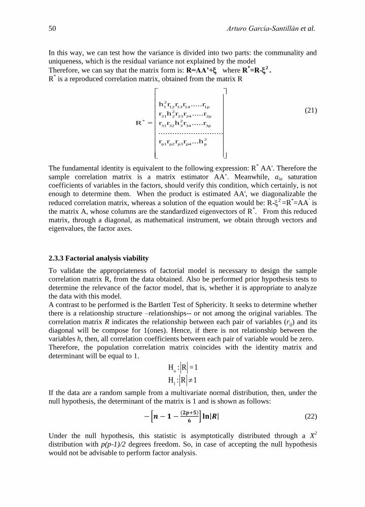
In this way, we can test how the variance is divided into two parts: the communality and

uniqueness, which is the residual variance not explained by the model

Therefore, we can say that the matrix form is: R=AA’+ where R*=R-

2 .

R* is a reproduced correlation matrix, obtained from the matrix R

2

1 12 13 14 1p

2

21 2 23 24 2p

* 2

31 32 3 34 3p

2

p1 p2 p3 p4 p

h r r r .....r

r h r r .....r

R = r r h r .....r

............................

r r r r ...h

(21)

The fundamental identity is equivalent to the following expression: R* AA'. Therefore the

sample correlation matrix is a matrix estimator AA’. Meanwhile, aia saturation

coefficients of variables in the factors, should verify this condition, which certainly, is not

enough to determine them. When the product is estimated AA', we diagonalizable the

reduced correlation matrix, whereas a solution of the equation would be: R-2

=R*=AA

’ is

the matrix A, whose columns are the standardized eigenvectors of R*. From this reduced

matrix, through a diagonal, as mathematical instrument, we obtain through vectors and

eigenvalues, the factor axes.

2.3.3 Factorial analysis viability

To validate the appropriateness of factorial model is necessary to design the sample

correlation matrix R, from the data obtained. Also be performed prior hypothesis tests to

determine the relevance of the factor model, that is, whether it is appropriate to analyze

the data with this model.

A contrast to be performed is the Bartlett Test of Sphericity. It seeks to determine whether

there is a relationship structure –relationships-- or not among the original variables. The

correlation matrix R indicates the relationship between each pair of variables (rij) and its

diagonal will be compose for 1(ones). Hence, if there is not relationship between the

variables h, then, all correlation coefficients between each pair of variable would be zero.

Therefore, the population correlation matrix coincides with the identity matrix and

determinant will be equal to 1.

o

1

H : R =1

H : R 1

If the data are a random sample from a multivariate normal distribution, then, under the

null hypothesis, the determinant of the matrix is 1 and is shown as follows:

(22)

Under the null hypothesis, this statistic is asymptotically distributed through a X2

distribution with p(p-1)/2 degrees freedom. So, in case of accepting the null hypothesis

would not be advisable to perform factor analysis.


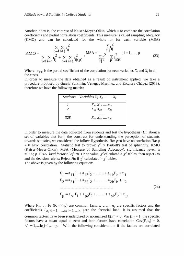
Another index is, the contrast of Kaiser-Meyer-Olkin, which is to compare the correlation

coefficients and partial correlation coefficients. This measure is called sampling adequacy

(KMO) and can be calculated for the whole or for each variable (MSA)

2rijj i i j

KMO =2 2

r + rij ij(p)j i i j j i i j

,

2riji¹j

MSA = ;i = 1,....., p2 2

r + rij ij(p)i¹j i¹j

(23)

Where: rij (p) is the partial coefficient of the correlation between variables Xi and Xj in all

the cases.

In order to measure the data obtained as a result of instrument applied, we take a

procedure proposed by García-Santillán, Venegas-Martinez and Escalera-Chávez (2013),

therefore we have the following matrix:

Students Variables X1 X2 . . . . . Xp

1

2

…..

328

X11 X12 …. x1p

X21 X22 …. x2p

………..

Xn1 Xn2 …. xnp

In order to measure the data collected from students and test the hypothesis (Hi) about a

set of variables that form the construct for understanding the perception of students

towards statistics, we considered the follow Hypothesis: Ho: ρ=0 have no corelation Ha: ρ

≠ 0 have correlation. Statistic test to prove: χ2, y Bartlett's test of sphericity, KMO

(Kaiser-Meyer-Olkin), MSA (Measure of Sampling Adecuacy), significancy level: α

=0.05; p <0.05 load factorial of .70 Critic value: 2 calculated > 2

tables, then reject Ho

and the decision rule is: Reject Ho if 2 calculated > 2

tables.

The above is given by the following equation:

X = a F + a F + .......... + a F + u1 11 1 12 2 11k k

X = a F + a F + .......... + a F + u2 21 1 22 2 22k k

....................................................................

X = a F + a F + .......... + a F + up pp1 1 p2 2 pk k

(24)

Where F1,. . . Fk (K << p) are common factors, u1,.... up are specific factors and the

coefficients ija ; i =1, . . . . ,p; j=1,....,k are the factorial load. It is assumed that the

common factors have been standardized or normalized E(Fi) = 0, Var (fi) = 1, the specific

factors have a mean equal to zero and both factors have correlation Cov(Fi,uj) = 0,

i=1,...,k; j=1,….,p. With the following consideration: if the factors are correlated


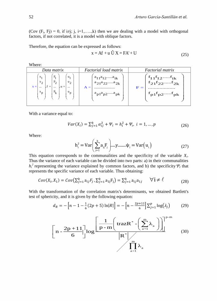
(Cov (Fi, Fj) = 0, if i≠j; j, i=1,…..,k) then we are dealing with a model with orthogonal

factors, if not correlated, it is a model with oblique factors.

Therefore, the equation can be expressed as follows:

x = Af + u Û X = FA' + U (25)

Where:

Data matrix Factorial load matrix Factorial matrix

x F u1 1 1

x F u2 2 2

, f = ,u =... ... ..x .

x F up pk

=

a a .....a11 12 ik

a a .....a21 22 2k

...................

a a .....ap1 p2 p

A =

k

f f .....f11 12 ik

f f .....f21 22 2k

...................

f f .....fp1 p2 p

F =

k

With a variance equal to:

= =

= 1 (26)

Where:

k2

i ij j i ij=1

h = Var a F .....y........ψ =V r u (27)

This equation corresponds to the communalities and the specificity of the variable Xi.

Thus the variance of each variable can be divided into two parts: a) in their communalities

hi2

representing the variance explained by common factors, and b) the specificityI that

represents the specific variance of each variable. Thus obtaining:

=

=

i (28)

With the transformation of the correlation matrix's determinants, we obtained Bartlett's

test of sphericity, and it is given by the following equation:

= 1

=

(29)

p-m

m*

aa=1

*

m

aa=1

1trazR - λ

p - m2p +11n - log

6 R

λ

(30)


3 Empirical Study

3.1 Finding and Discussions

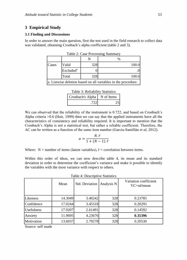
In order to answer the main question, first the test used in the field research to collect data

was validated, obtaining Cronbach’s alpha coefficient (table 2 and 3).

Table 2: Case Processing Summary

N %

Cases Valid 328 100.0

Excludeda 0 .0

Total 328 100.0

a. Listwise deletion based on all variables in the procedure.

Table 3: Reliability Statistics

Cronbach's Alpha N of Items

.722 25

We can observed that the reliability of the instrument is 0.722, and based on Cronbach’s

Alpha criteria >0.6 (Hair, 1999) then we can say that the applied instruments have all the

characteristics of consistency and reliability required. It is important to mention that the

Cronbach’s Alpha is not a statistical test, but rather a reliable coefficient. Therefore, the

AC can be written as a function of the same item number (García-Santillán et al, 2012).

=

1 1

Where: N = number of items (latent variables), ř = correlation between items.

Within this order of ideas, we can now describe table 4, its mean and its standard

deviation in order to determine the coefficient’s variance and make it possible to identify

the variables with the most variance with respect to others.

Table 4: Descriptive Statistics

Mean

Std. Deviation

Analysis N

Variation coefficient

VC=sd/mean

Likeness 14.3049 3.40242 328 0.23785

Confidence 17.0244 3.45518 328 0.20295

Usefulness 17.9207 2.61491 328 0.14592

Anxiety 11.9695 4.23676 328 0.35396

Motivation 13.6037 2.79278 328 0.20530

Source: self made


Based on the results described in Table 4, it can be seen that the variable ANXIETY

(35.39%) is the largest compared to the rest of the variables that show similar behavior

(among 14.59% to 23.78%). After collecting the data, and in order to validate whether the

statistical technique of factor analysis can explain the phenomena studied, we first

conducted a contrast from Bartlett's test of sphericity with Kaiser (KMO) and Measure

Sample Adequacy (MSA) to determine whether there is a correlation between the

variables studied and whether the factor analysis technique should be used in this case.

Table 5 shows the results.

Table 5: KMO and Bartlett's Test

Kaiser-Meyer-Olkin Measure of Sampling Adequacy. .592

Bartlett's Test of Sphericity Approx. Chi-Square 390.552

df 10

Sig. 0.000

Source: self made

As we already know, Bartlett’s test of sphericity allows the null hypothesis that the

correlation matrix is an identity matrix, whose acceptance involves rethinking the use of

principal component analysis as the KMO is > 0.5, in which case the factor analysis

procedure should not be used. Now, observing the results in the table above; the KMO

statistic has a value of 0.592 which is more than >0.5 and Bartlett sphericity test with X2

=390.552 with 10 df and sig. 0.000, indicating that the data is adequate to perform a factor

analysis. Therefore a factor analysis can be made that allows answering the research

question.

The results obtained from the correlation matrix are shown in Table 6; we observe the

behavior of each variable with respect to others. The criteria for determining low

correlation is the higher number, lower versus higher determining the correlation, then

one can predict the degree of intercorrelation between the variables.

Table 6: Correlation Matrixa

Likeness Anxiety Confidence Motivation Usefulness

Correlation Likeness 1.000

Anxiety -.153 1.000

Confidence .540 -.321 1.000

Motivation .304 .354 .154 1.000

Usefulness .463 -.053 .542 .131 1.000

a. Determinant = .300

Source: self made

In the above table we see that the determinant is high (0.300) indicating a low degree of

intercorrelation between the variables (<0.5) however, it shows a positive correlation

(except: anxiety vs. likeness -.153; anxiety vs. confidence -.321 and anxiety vs. usefulness

-0.053), this should be taken with caution when wording the conclusions. Just to mention

some examples of significant correlations (the highest) should be correlated: Confidence


vs. Likeness (0,540), Confidence vs. Usefulness (0,542) and the rest of the variables are

presented in the order of 0.13 to 0.46 their respective correlations between the variables

involved in this study.

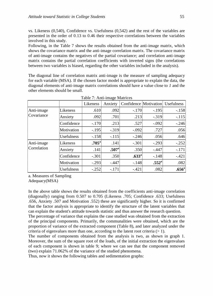
Following, in the Table 7 shows the results obtained from the anti-image matrix, which

shows the covariance matrix and the anti-image correlation matrix. The covariance matrix

of anti-image contains the negatives of the partial covariance; and correlation anti-image

matrix contains the partial correlation coefficients with inverted signs (the correlations

between two variables is biased, regarding the other variables included in the analysis).

The diagonal line of correlation matrix anti-image is the measure of sampling adequacy

for each variable (MSA). If the chosen factor model is appropriate to explain the data, the

diagonal elements of anti-image matrix correlations should have a value close to 1 and the

other elements should be small.

Table 7: Anti-image Matrices

Likeness Anxiety Confidence Motivation Usefulness

Anti-image

Covariance

Likeness .610 .092 -.170 -.195 -.158

Anxiety .092 .701 .213 -.319 -.115

Confidence -.170 .213 .527 -.092 -.246

Motivation -.195 -.319 -.092 .727 .056

Usefulness -.158 -.115 -.246 .056 .646

Anti-image

Correlation

Likeness .705a .141 -.301 -.293 -.252

Anxiety .141 .507a .350 -.447 -.171

Confidence -.301 .350 .633a -.148 -.421

Motivation -.293 -.447 -.148 .552a .082

Usefulness -.252 -.171 -.421 .082 .656a

a. Measures of Sampling

Adequacy(MSA)

In the above table shows the results obtained from the coefficients anti-image correlation

(diagonally) ranging from 0.507 to 0.705 (Likeness .705; Confidence .633; Usefulness

.656, Anxiety .507 and Motivation .552) these are significantly higher. So it is confirmed

that the factor analysis is appropriate to identify the structure of the latent variables that

can explain the student's attitude towards statistic and thus answer the research question.

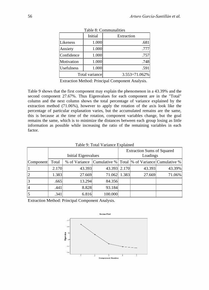
The percentage of variance that explains the case studied was obtained from the extraction

of the principal components. Primarily, the communalities were obtained, which are the

proportion of variance of the extracted component (Table 8), and later analyzed under the

criteria of eigenvalues more than one, according to the latent root criteria (> 1).

The number of components obtained from the analysis is two, as shown in graph 1.

Moreover, the sum of the square root of the loads, of the initial extraction the eigenvalues

of each component is shown in table 9; where we can see that the component removed

(two) explain 71.062% of the variance of the studied phenomena.

Thus, now it shows the following tables and sedimentation graphs:


Table 8: Communalities

Initial Extraction

Likeness 1.000 .681

Anxiety 1.000 .777

Confidence 1.000 .757

Motivation 1.000 .748

Usefulness 1.000 .591

Total variance 3.553=71.062%

Extraction Method: Principal Component Analysis.

Table 9 shows that the first component may explain the phenomenon in a 43.39% and the

second component 27.67%. Thus Eigenvalues for each component are in the "Total"

column and the next column shows the total percentage of variance explained by the

extraction method (71.06%), however to apply the rotation of the axis look like the

percentage of particular explanation varies, but the accumulated remains are the same,

this is because at the time of the rotation, component variables change, but the goal

remains the same, which is to minimize the distances between each group losing as little

information as possible while increasing the ratio of the remaining variables in each

factor.

Table 9: Total Variance Explained

Component

Initial Eigenvalues

Extraction Sums of Squared

Loadings

Total % of Variance Cumulative % Total % of Variance Cumulative %

1 2.170 43.393 43.393 2.170 43.393 43.39%

2 1.383 27.669 71.062 1.383 27.669 71.06%

3 .665 13.294 84.356

4 .441 8.828 93.184

5 .341 6.816 100.000

Extraction Method: Principal Component Analysis.


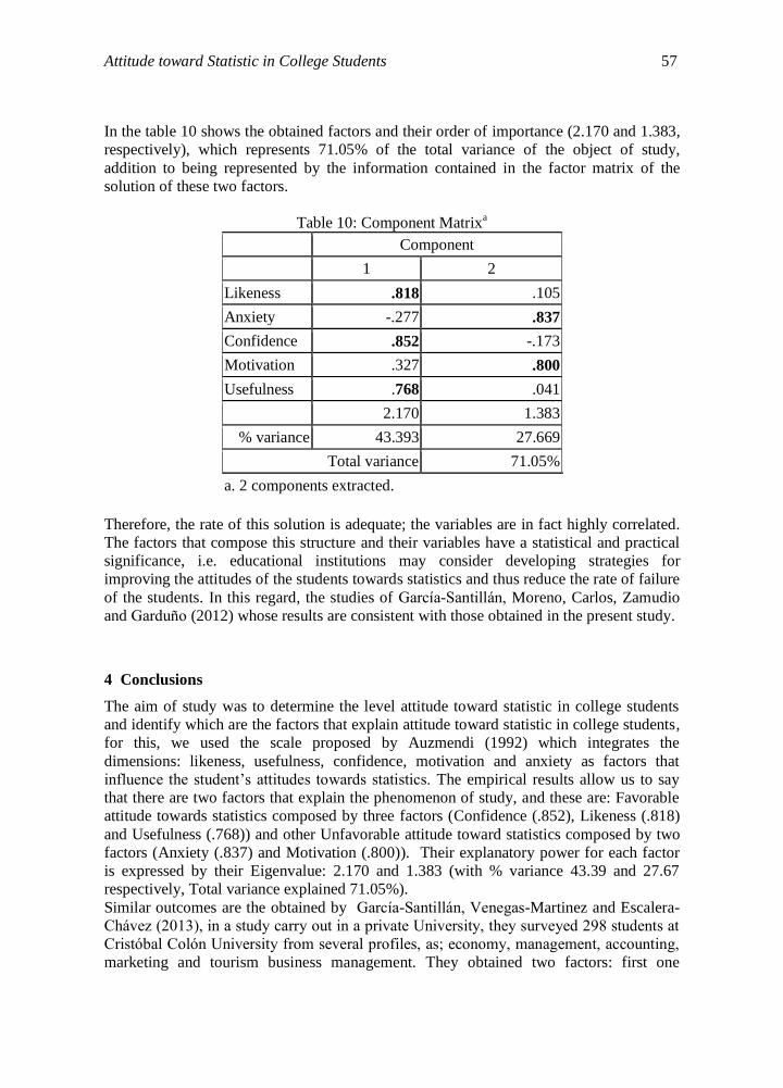
In the table 10 shows the obtained factors and their order of importance (2.170 and 1.383,

respectively), which represents 71.05% of the total variance of the object of study,

addition to being represented by the information contained in the factor matrix of the

solution of these two factors.

Table 10: Component Matrixa

Component

1 2

Likeness .818 .105

Anxiety -.277 .837

Confidence .852 -.173

Motivation .327 .800

Usefulness .768 .041

2.170 1.383

% variance 43.393 27.669

Total variance 71.05%

a. 2 components extracted.

Therefore, the rate of this solution is adequate; the variables are in fact highly correlated.

The factors that compose this structure and their variables have a statistical and practical

significance, i.e. educational institutions may consider developing strategies for

improving the attitudes of the students towards statistics and thus reduce the rate of failure

of the students. In this regard, the studies of García-Santillán, Moreno, Carlos, Zamudio

and Garduño (2012) whose results are consistent with those obtained in the present study.

4 Conclusions

The aim of study was to determine the level attitude toward statistic in college students

and identify which are the factors that explain attitude toward statistic in college students,

for this, we used the scale proposed by Auzmendi (1992) which integrates the

dimensions: likeness, usefulness, confidence, motivation and anxiety as factors that

influence the student’s attitudes towards statistics. The empirical results allow us to say

that there are two factors that explain the phenomenon of study, and these are: Favorable

attitude towards statistics composed by three factors (Confidence (.852), Likeness (.818)

and Usefulness (.768)) and other Unfavorable attitude toward statistics composed by two

factors (Anxiety (.837) and Motivation (.800)). Their explanatory power for each factor

is expressed by their Eigenvalue: 2.170 and 1.383 (with % variance 43.39 and 27.67

respectively, Total variance explained 71.05%).

Similar outcomes are the obtained by García-Santillán, Venegas-Martinez and Escalera-

Chávez (2013), in a study carry out in a private University, they surveyed 298 students at

Cristóbal Colón University from several profiles, as; economy, management, accounting,

marketing and tourism business management. They obtained two factors: first one


composed of three elements: usefulness, confidence, liking and other incorporates two

elements: anxiety and motivation. The values of this last factor indicate if the student

anxiety increased, decreased motivation and their explanatory power for each factor are

expressed by their Eigenvalue 2.351 and 1.198 (with % variance 47.016 and 23.964

respectively, Total variance 71.08%)

These results are consistent with those presented by Auzmendi (1992) who notes that the

factors that have the greatest influence are those related to motivation, liking and the

utility.

Finally, the factor the most explained the student attitude toward statistic is: Confidence,

following of Likeness and Usefulness that integrate the first component that explain

43.39% of variance and Anxiety and Motivation that integrate the second component that

explain 27.67% of total variance.

ACKNOWLEDGEMENTS: The authors are very grateful to the anonymous reviewer

for suggestions and Universidad Politécnica de Aguascalientes for all their help and

support.

References

[1] Auzmendi, E. (1991). Evaluación de las actitudes hacia la estadística en alumnos

universitarios y factores que las determinan. Tesis doctoral (no publicada).

Universidad de Deusto, Bilbao.

[2] Beins, B.C. (1985). Teaching the relevance of statistics trough consumer-oriented

research. Teaching of Psychology 12,168-169

[3] Blanco, A. (2004). Enseñar y aprender estadística en las titulaciones universitarias

de ciencias sociales: apuntes sobre el problema desde una perspectiva pedagógica,

“Hacia una Enseñanza Universitaria Centrada en el Aprendizaje”, Universidad

Pontificia de Comillas, Madrid, España.

[4] Blanco, A. (2008). Una revisión crítica de la investigación sobre las actitudes de los

estudiantes universitarios hacia la Estadística. Revista Complutense de Educación,

19 (2), 311-330.

[5] Chang, A. S. (1990, July). Streaming and Learning Behavior. Paper presented at the

Annual Convention of the International Council of Psychologists, Tokyo, Japan

(ERIC Reproduction Service No. ED 324092).

[6] Cherian, V. I., y Glencross, M. J. (1997). Sex, socio-economic status, and attitude

toward applied statistics among postgraduate education students. Psychological

Reports, 80, 1385-1386.

[7] Elmore, P.B. y Lewis, E.L. (1991). Statistics and computer attitudes and

achievement of students enrolled in applied statistrics: Effect of a Computer

laboratory. Chicago: American Educational Research Association Annual Meeting.

[8] Gal, I. y Ginsburg, L. (1994). The Role of Beliefs and Attitudes in Learning

Statistics: Towards an Assesment Framework. Journal of Statistics Education, 2, (2)

Obtained of: http://www.amstat.org/publications/jse/v2n2/gal.html.

[9] Gal, I., Ginsburg, L. y Schau, C. (1997). Monitoring Attitudes and Beliefs in

Statistics Education. En Gal, I. y Garfield, J. (Eds.) (1997). The Assessment


Challenge in Statistics Education. Amsterdam, IOS Press and International

Statistical Institute.

[10] García-Santillán, A.; Escalera-Chávez, M.; and Córdova Rangel, A.; (2012).

Variables to measure interaction among mathematics and computer through

structural equation modeling. Journal of Applied Mathematics and Bioinformatics

2(3), 51-67.

[11] García-Santillán, A.; Moreno, E.; Carlos, J.; Zamudio, J. & Garduño, J. (2012).

Cognitive, Affective and Behavioral Components that explain Attitude toward

Statistics. Journal of Mathematics Research. 4(5), 8-16.

[12] García-Santillán, A.; Venegas-Martínez, F.; Escalera-Chávez, M. (2013). An

exploratory factorial analysis to measure attitude toward statistic. Empirical study in

undergraduate students. International Journal of Research and Reviews in Applied

Sciences, 14, (2), 356-366.

[13] Katz, B. M. y Tomazic, T.C. (1988). Changing student’s attitude toward statistics

through a nonquatitative approach. Psichological Reports, 62, 658.

[14] McLeod D. (1992). Research on affect in mathematics education: a

reconceptualization, in .Grows (Ed.), Handbook of Research on Mathematics

Teaching and Learning (pp.575-596). McMillan Publishing Company.

[15] Mondéjar, J., Vargas, M., & Bayot, A. (2008). Measuring attitude toward statistics:

the influence of study processes. Electronic Journal of Research in Educational

Psychology, 6(3), 729-748.

[16] Phillips, J.L. (1980): La lógica del pensamiento estadístico. México, el Manual

Moderno.

[17] Roberts, D.M. y Bilderback, E.M. (1980). Realibility and Validity of a "Statistics

Attitude Survey". Educational and Psychological Measurement, 40, 235-238.

[18] Roberts, D.M. y Saxe, J.E. (1982). Validity of Statistics Attitude Survey: A Follow-

Up Stuty. Educational and Psychological Measurement, 42, 907-912.

[19] Roberts, D.M. y Reese, C.M. (1987). A Comparison of Two Scales Measuring

Attitudes Towards Statistics. Educational and Psychological Measurement, 47, 759-

764.

[20] Sánchez-López, C.R. (1996). Validación y análisis ipsativo de la Escala de

Actitudes hacia la Estadística (EAE). Análisis y modificación de conducta, 22, 799-

819.

[21] Schau, C., Stevens, J., Dauphinee, T.L. and Del Vecchio, A. (1995). The

development and validation of the Survey Attitudes Toward Statistics. Educational

and Psychological Measurement, 55(5), 868-875.

[22] Schutz, P.A.; Drogosz, L.M.; White, V.E. and Diestefano, C. (1997). Prior

Knowledge, Attitude and Strategy Use in an Introduction to Statistics Course. Paper

presented at the Annual Meeting of the American Educational Research Association.

Chicago.

[23] Sutarso, T. (1992). Some variables in relation to students´anxiety in learning

statistics. Paper presented at the Annual Meeting of the Mid-South Educational

Research Association, Knoxville (ERIC Document Reproduction Service nº

ED353334).

[24] Vanhoof, S., Castro, A.E., Onghena, P., Verschaffel, L., Van Dooren, W y Van Den

Noortgate, W. (2006). Attitudes toward statistics and their relationship with short-

and long-term exam results Journal of Statistics Education, 14(3). Obtained of:

www.amstat.org/publications/jse/v14n3/vanhoof.html.

http://www.amstat.org/publications/jse/v14n3/vanhoof.html


[25] Wise, S.L. (1985). The development and validation of a scale measuring attitudes

toward statistics. Educational and Psychological Measurement, 45, 401-405.

[26] Woehlke, P.L. (1991). An examination of the factor structure of Wise’s Attitude

Toward Statistics scale. Annual Meeting of the American Educational Research

Association, Chicago, IL, USA. (ERIC Document Reproduction Service No.

ED337500).

attitude toward statistic in college students (an ... 2_1_4.pdf · universidad politécnica de...

Documents