atek adr 10 series - kanooneabzar.com

OPERATION

MANUAL

Atek ADR 10 Series

HIGH PERFORMANCE

DIGITAL READOUT

فروشگاه کانون ابزارتلفن : 00 39 39 66 021موبایل : 3023 147 0912

www.ali5.ir

[1]

Index 1. ATEK DIGITAL READOUT SYSTEMS........................................................................................................................... 3

1.1. ATEK linear encoder and digital coordinate readout unite usage advantages ................................................. 3

1.2. ATEK Magnetic Linear Encoder ......................................................................................................................... 3

2. TECHNICAL PARAMETERS......................................................................................................................................... 4

3. SYSTEM SETUP .......................................................................................................................................................... 8

3.1. Language Selection ........................................................................................................................................... 8

3.2. Resolution Setup ............................................................................................................................................... 8

3.3. Direction Setup ................................................................................................................................................. 9

3.4. Machine Tool Selection ..................................................................................................................................... 9

3.5. Compansation Selection ................................................................................................................................... 9

3.6. Advanced Settings ............................................................................................................................................. 9

3.6.1. Digit On-Off ............................................................................................................................................. 10

3.6.2. Axis Addition ........................................................................................................................................... 10

3.6.3. 4. Axis Type ............................................................................................................................................. 10

3.6.4. Calculator Decimal Setup ........................................................................................................................ 10

3.6.5. Probe Logic Level Setup .......................................................................................................................... 11

3.6.6. Buzzer Close ............................................................................................................................................ 11

3.6.7. Return to Factory Settings ...................................................................................................................... 11

3.7. Test .................................................................................................................................................................. 11

3.7.1. Display Test ............................................................................................................................................. 11

3.7.2. Eeprom Test ............................................................................................................................................ 12

3.7.3. Keyboard Test ......................................................................................................................................... 12

3.7.4. CPU Test .................................................................................................................................................. 12

3.7.5. Relay Test ................................................................................................................................................ 12

4. Basic Functions ....................................................................................................................................................... 13

4.1. Measurement System Change ........................................................................................................................ 13

4.2. Operation Mode Selection .............................................................................................................................. 13

4.3. Quick Zero Axis Values .................................................................................................................................... 13

4.4. Manuel Value Setting for Each Axis: ............................................................................................................... 13

4.5. Setting Half Value of The Display Value (Milling, Bohrwerk) .......................................................................... 14

4.6. Diameter Mode (Lathe):.................................................................................................................................. 14

4.7. Center Find (Milling, Bohrwerk) ...................................................................................................................... 14

4.8. Simple Calculation on Axis Values:.................................................................................................................. 16

4.9. Undo Function ................................................................................................................................................. 16

4.10. Activate the 4th Axis ................................................................................................................................... 16

4.11. Display Angle on the 4th Axis ...................................................................................................................... 17

[2]

4.12. Sleep Mode: ................................................................................................................................................ 17

5. ADVANCED FUNCTIONS ......................................................................................................................................... 18

5.1. To Find Zero Point of the Machine Tool.......................................................................................................... 18

5.1.1. Ruler Zero Point: ..................................................................................................................................... 18

5.1.2. Mechanical Zero Point: ........................................................................................................................... 19

5.2. Error Compensation Function: ........................................................................................................................ 20

5.2.1. Linear Error Compensation Function: ..................................................................................................... 20

5.2.2. Segmented Error Compansation Function: ............................................................................................. 21

5.3. Travel Limit: ..................................................................................................................................................... 23

5.4. Axis Addition (Lathe, Bohrwerk) ..................................................................................................................... 24

5.5. Shrink Function: .............................................................................................................................................. 25

5.6. Calculator Function: ........................................................................................................................................ 26

5.6.1. To Transfer the Calculated Values To The Axes: ..................................................................................... 26

5.6.2. To Transfer The Axis Values To Calculator: ............................................................................................. 27

5.7. Datum Point Memory: .................................................................................................................................... 28

5.8. Bolt Hole Circle (Divisor) (Milling) ................................................................................................................... 32

5.9. Bolt Hole Line Function (Milling) ..................................................................................................................... 34

5.10. Smooth Radius (Milling) .............................................................................................................................. 36

5.11. Simple Radius (Milling) ................................................................................................................................ 39

5.12. Linear Hole Patterns (Milling) ..................................................................................................................... 41

5.13. Frame Hole Patterns (Milling) ..................................................................................................................... 43

5.14. Rectangular Pocket (Milling) ....................................................................................................................... 45

5.15. Work Piece Angle Measuring (Milling) ........................................................................................................ 47

5.16. Touch Probe (Milling, Bohrwerk) ................................................................................................................ 48

5.16.1. Zero the Axis / Setting Half Value of the Display Value .......................................................................... 48

5.16.2. Find Center .............................................................................................................................................. 49

5.16.3. Measurement .......................................................................................................................................... 50

5.17. Tool Diameter Compansation (Milling) ....................................................................................................... 52

5.18. Tool Storeroom (Lathe) .............................................................................................................................. 53

5.19. Taper Angle Measurement (Lathe) ............................................................................................................. 56

5.20. Digital Filter (Vibration Filter) ..................................................................................................................... 57

5.21. Inclined Z Axis Machining (Milling) ............................................................................................................. 58

5.22. EDM Depth Control Function (Erosion) ...................................................................................................... 60

5.23. HOLD Function ............................................................................................................................................ 62

5.24. Data Transfer by RS – 232 Port ................................................................................................................... 63


www.ali5.ir

[3]

1. ATEK DIGITAL READOUT SYSTEMS

1.1. ATEK linear

encoder and

digital

coordinate

readout unit

usage

advantages

1.2. ATEK Magnetic

Linear Encoder

New 2, 3 and 4 axis available ADR 10 Series Digital Readouts can meet the

application in all machine tools with maximum performance and it includes

features that are essential for increasing productivity. With high-capacity

memory it is possible to save 1000 pcs programs and for the lathes 1000

pcs tool memory. 5 different language choices are existed as Turkish,

English, German, Spanish and Portuguese. Connection opportunity by

contact probe is also available. With 8+1 digit display and standard

resolution values with user designated resolution, ADR10 is designed for

your all requires.

ADR 10;

- Minimizing production time, increasing productivity.

- Scrap Cost Saving.

- More Accurate Positioning.

- More Quality Parts.

- 80% Reduced Process time.

- Amortizing in a Short Time.

For the best performance please use ATEK Linear Encoders. ATEK MLC

Series magnetic linear scales presents to their user’s high accuracy and

usage advantages. The magnetic systems never influenced negatively from

the environmental conditions as dust, chip, humidity and cutting fluid, they

work without any problem. Because of the contactless working there is no

friction, they have unlimited lead time mechanically, they work without

any mechanical problem and maintenance.

Visit our web site for linear scale options and details.

www.ateksensor.com


www.ali5.ir

http://www.ateksensor.com/

[4]

1. TECHNICAL PARAMETERS

TECHNICAL SPECIFICATIONS

Axis Number 2, 3, 4

Display 8 Digit + 1 Sign (-) Digit, Green, Touring (-) Sign

Display Resolution 0.1 µm, 0.2 µm, 0.5 µm, 1 µm, 5 µm, 10 µm, 25 µm

Or the user can designate as requested.

Input Signal Available Push Pull or TTL

A,B,Z (Line Driver A, B, Z, /A, /B, /Z) Incremental Encoder Signals

Mass 3 Kg

Power Supply Voltage 85 – 265 V AC 50/60Hz.

Storage Temperature - 25 ~ 65 °C

Operation Temperature -10 ~ 45 °C

Relative Humidity %20 - %85

Protection Class IP54

Dimensions( H x W x T ) 202mm x 320mm x 84mm

Housing Aluminum Injection Housing

Diameter Limits - 99999,999 mm ~ 99999,999 mm

320

202

[5]

Metric / Inch

measurement selection Absolute / Incremental

Mode Selection Shrink

X Axis Zero Button Y Axis Zero Button Z Axis Zero Button

W Axis Zero Button

X Axis Selection Y Axis Selection Z Axis Selection

W Axis Selection

Addition Multipication Substraction Button Division

Square Root Button Equal

ENTER

Sign Changing Button

½ Function Button

Divisor

4 Axis Activation

Button

Calculator

- Numeric Buttons

Undo

Sleep Mode

X Axis

(Axis 1)

Y Axis

(Axis 2)

Z Axis

(Axis 3)

Info Screen

and W axis

(Axis 4)

Cosinus Function Sinus Function Tangant Function

Tool Enter Button

(Lathe)

Screen Renew Ratio and

EDM Function

User Zeros

Recall (lathe) Trape Angle and

Eccentricity Measurement

Bolt Hole Line Radius Functions

Travelling Button

Clear Button Delete Arc Trigonometric

Function

Decimal Point button


www.ali5.ir

[6]

While Connection;

▪ Never Make Connection Under Energy.

▪ Check the On / Off Switch is “Off”.

▪ Check the power voltage if convenient values.

▪ Use only the power cable which is given with the product.

▪ Check the ground connections.

▪ Don’t use in strong magnetic field.

▪ Don’t use in high temperature and humidity environments.

▪ Install the display as vertical in the high which user can use the keyboard and see the screen.

Note: 4 Axis ADR 10-4 Type DRO Gear Panel View.

Contact

Probe

connection

Encoder

Connection

RS -232

Connection

Ground

Connection

Buzzer

Voice

Power Cable

Connection

On / Off

Switch

1A Insure

WARNING!

While installation of the device, please switch all

machine energy off and follow the manual directions.

[7]

Encoder Connections (Differential)

Encoder Connections

RS – 232 Output Port Connection

Contact Probe Connection

Note: While using single contact probe “Signal-” pin must be empty.

Pin Number 1 2 3 4 5 6 7 8 9

Signal A /B +V 0V /A B /Z Z Shield

Pin Number 1 2 3 4 5 6 7 8 9

Signal A Empty +V 0V Empty B Empty Z Shield

Pin Number 1 2 3 4 5 6 7 8 9

Signal Empty Rx Tx Empty 0V Empty Empty Empty Shield

Pin Number 1 2 3 4 5 6 7 8 9

Signal Signal+ Empty +V 0V Signal- Empty Empty Empty Shield

Signal (for SINO) Empty 0V Empty Empty Empty Signal+ +V Signal- Shield

1 2 3 4 5

6 7 8 9

1 2 3 4 5

6 7 8 9

1 2 3 4 5

6 7 8 9

1 2 3 4 5

6 7 8 9


www.ali5.ir

[8]

2. SYSTEM SETUP

To enter system setup, when ADR-10 first energized (power connections completed and on/off switch turned “on”)

press “ENTER” button ( ) for a while. You will see “LANGUAGE” word as first when you are in system setup menu.

For MENU traveling buttons can be used.

3.1. Language Selection It is the first selection of system setup. The numeric buttons can be used for language selection.

In data display “LANGUAGE” and in X axis display language options are written. Language selection can be done by

numeric buttons. After selection please press “ENTER” to save.

3.2. Resolution Setup

After selection language, by pressing button you can enter the resolution setup for X axis. The included

resolution options are displayed as first.

In data screen “RESOLION X” words are seen while the resolution value is seen on X axis. To save the resolutions

please press to enter.

* “9” button is used for user determinate resolution.

To enter user determinate resolution after pressing “9” button please press “ENTER” button. To enter a value press

“Sx” button and enter the resolution value and press enter to save.

You can turn to system setup menu by button.

For the other axes you can repeat the same operation for resolution setup.

Numeric Button 0 1 2 3 4

Language Option Turkish English German Spanish Portuguese

Numeric Button 0 1 2 3 4 5 6 7 8 9

Resolution 5 µm 1 µm 2 µm 10 µm 25 µm 0,1 µm 0,2 µm 0,5 µm *

[9]

Using 4th Axis for Angle Display

For angle measurement with 4th axis (W axis) when you are in “RESOLION W” please press “9” button and press

“ENTER” to enter the pulse number of the encoder. Press “ENTER” again to save. After this in “ADVANCED” menu “W

TYPE” option must be select as 1 – rotary. “ADVANCED” menu will be told detailed in the fallowing pages.

2.3. Direction Setup It determinates the measuring direction according to encoder movement direction.

For positive measuring direction, press “1” button. You will see “1” value in X axis. For negative measuring

direction, please press “0” button. “-1” value will be seen on X axis. Press “ENTER” to save.

You can repeat the same buttons for the other axes.

2.4. Machine Tool Selection This menu is used to select the type of the machine tool which Digital Readout used on.

Please press “ENTER” button after machine tool selection.

2.5. Compansation Selection Compansation selection is setup by system setup menu.

By up-down button the “COMPNSTN” writing is found please select linear compensation by “0” button and select

segmented compensation by “1” button. Save the selected compensation by pressing “ENTER” button.

2.6. Advanced Settings You can receive to Advanced Settings by “System Setup” menu.

After see “ADVANCED” writing, press “ENTER” to enter the menu.

Numeric Button 0 1 2 3 4

Machine Type Milling Lathe Grinding Bohrwerk Spark

Erosion

[10]

2.6.1. Digit On-Off

It is in the “Advanced Setting” menu.

You can determine the closed digit number by “Hide X” menu. You can close digit numbers up to 5 digits. Please

enter the digit number which will be closed by keyboard and press “ENTER” to save

Please repeat the same way for the other axes.

2.6.2. Axis Addition

Only for lathe and bohrwerk machine tools the axis addition can be used.

You can use this option by “Advanced Setting”

By “1” button you can active and “0” button you can passive. On lathes it adds and Z axis. On bohrwerk machine

tools it adds Z and W axis.

In this menu if addition is active, on lathes Z axis, on Bohrwerks W axis can’t be change by manuel.

2.6.3. 4th Axis Type

The encoder type which will be used on 4th axis means W axis must be enter.

If a rotary encoder will be used press “1” button. On X axis “1” writing and on Y axis “rot” writing will be seen. If a

linear encoder will be used “0” button must be pressed. On X axis “0” writing and on Y axis “Lin” writing will be seen.

2.6.4. Calculator Decimal Setup

This menu determines the decimal number of the calculations on the calculator.

3 or 4 digits can be seen after point. The decimal number can be entering by keyboard. After press “ENTER” to save

the value.

[11]

2.6.5. Probe Logic Level Setup

It can be needed to change according to used probe.

If there is a signal after probe contact (High-Active) must change as “1”, if there is no any signal (Low-Active) must be

change as “0”. Press “ENTER” to save.

2.6.6. Buzzer Close

Buzzer voice can be closed by this menu.

It can be closed by “1” button and can be opened by “0” button.

2.6.7. Return to Factory Settings It is used to reset all functions changes.

In the menu, to return factory settings please press to “Enter” button. “SURE” writing is seen. Press again to

“ENTER”. “WAIT” writing is seen and after a while it turns to fabric setup.

2.7. Test In system setup menu the device can be tested. You can make display, eeprom test, CPU test, and Relay Test.

Press “Enter” button to enter the menu.

2.7.1. Display Test

It exists in test menu. It can be active by “ENTER” button.

After pressing “Enter” button it clicks all the LED and display segments. Only “Probe” LED can’t be test. To stop the

testing press button.

[12]

2.7.2. Eeprom Test

If Eeprom Works correct when you press “ENTER” button you will see “1” writing.

2.7.3. Keyboard Test

It exists in test menu. You can active it by “ENTER” button.

After activation you have to see different number by for each pressed buttons. To turn back, press button.

2.7.4. CPU Test

When you press “Enter” button CPU data can be seen.

On X axis, it shows drawer speed in Hertz unit, on Y axis drawer flash memory in Byte unit, on Z axis RAM in byte

unit.

2.7.5. Relay Test

By pressing “Enter” button this test can be done.

For each “ENTER” pressing the relay will be push and pull.

[13]

4. Basic Functions 4.1. Measurement System Change

By the button on the keyboard the measurement unit as Metric or Inch system can be selected.

Fort his operation button is used. For each pressing the measurement system is changed. The used

measurement systems can be transfer to the user by LED’s.

Example:

Using Metric Measurement System → Using Inch Measurement System→

4.2. Operation Mode Selection

Operation Mode can be selected by ABS/INC button on the keyboard. 2 different coordinate display systems are

supported.

- Absolute Operation Mode

- Incremental Operation Mode

For each pressing the operation mode is changed. The used measurement system is transfer to user by

LED’s. In the same time it is showed on data display.

Example:

Using Absolute Operation Mode →

Using Incremental Operation Mode →

4.3. Quick Zero Axis Values

Axis values can be zero by the zero buttons of the ach axes.

To zero X axis button is used, To zero Y axis button is used, to zero Z axis, button is used and to zero W

axis button is used.

Example: To zero X axis;

→ →

4.4. Manuel Value Setting for Each Axis:

It is used to setting value to the axes as manuel.

The axis which will be value setting should be selected by the “Axis Selection Button, the value should be set and

ENTER button should be pressed. To select X axis , to select Y axis to select Z axis and to select W axis

nx button should be pressed and enter is pressed.

[14]

Example: To setting 26.100 mm for X axis;

→ →

4.5. Setting Half Value of the Display Value (Milling, Bohrwerk)

With the included keyboard you can get the half value of the axis you want. Firstly the select the axis which you want

to get half value and press ½ function button.

Example: To get half value of the X axis which shows 50.000;

→ →

4.6. Diameter Mode (Lathe):

With this mode, designed for lathe machines the measured value is showed as 2 times. It is valid on X axis. To

activate this function X axis is selected and ½ button is pressed. When the function is activated, “Diameter Mode”

LED signs.

Example: On X axis which shows 50.000 value to activate diameter mode;

→ →

4.7. Center Find (Milling, Bohrwerk) It is used to find centre of the work piece on XY plane according to teached points. The 4 point of the work piece

must be teached.

Please press “5” button and press enter to enter the function. Contact the tool edge on the first point on X axis as

“Position 1” and press enter to save. Contact the tool edge on Point 2 for position 2 and press enter. For 3 point

contact the tool edge to Point 3 on Y axis for position 3 and press enter. As last contact the tool edge for Point 4 and

press enter to save. You will see “OK” writing on the screen. When you press enter you will see the coordinates to

find the centre by moving. When you move the table up to make zero the coordinates you will be found the centre.

X

Position 4

Position 3

Position 1 Position 2

Position 4

Position 3


X

Y Y

[15]

Example:

→ → →

→ →

→ →

→ →

→ →

→ →

→ When you move up to reset axis value zero you can find the centre of the work piece.

To find the centre of the drawing on the

left.

Position 4

Position 3


Y

Tool edge is bringed to

“Position 1”


“Position 2”


“Position 3”


“Position 4”

[16]

4.8. Simple Calculation on Axis Values:

It is possible to make simple calculation as addition, subtraction, division and multiplication on axis values. It can be

done without activation of calculator. Firstly the axis which the calculation will be done must be selected. Press the

calculation button (+,-,/,* ). And then;

Example: To divide by 3 the X axis value;

→ →

4.9. Undo Function

After transferring the axis value as manuel or after making simple calculations to return the last value this function is

used. For this function firstly select the axis and press button and press enter. If you press button again you

will be canceled the operation.

Example: To turn to old values on X axis;

→ →

4.10. Activate the 4th Axis

In 4 axis digital readouts you can activate or deactivate the 4th axis. The axis 4 button is used for this operation

Example: To activate the 4th axis;

→ →

Example: To deactivate the 4th axis;

→ →

[17]

4.11. Display Angle on the 4th Axis To display angle on 4th axis by “system setting” menu the encoder pulse number must be entered as W resolution.

And again by “system setting” menu, rotary type must be selected. You can also see this setting on system setting as

detailed.

The angle can be set as Degree or Degree.minute.second. To make passing please press “Sw” button and “Tan/F3”

button accordingly.

Example: To Change Degree Angle as Degree.minute.second;

→ →

4.12. Sleep Mode: When the screen is on sleepy mode all the buttons are turned off except “HOLD” button. By this way 3th person

interfere will be prevented. Although the buttons are turned off, the signals will be process. If you change the table

place it senses this changing and if in the normal mode it uses the last position.

In the brake times and after works the device can be sleepy mode until beginning to work again.

You can pass “Sleepy Mode” by “HOLD” button and it is possible to exit by the same “HOLD” button.

Example: To pass to “Sleepy” mode and to exit;

→ →

→

[18]

5. ADVANCED FUNCTIONS

5.1. To Find Zero Point of the Machine Tool It is used not to lost time by measuring the work pieces one by one. The zero point will not be deleted after energy

cuttings. But for the high accuracy it will be better to revise for each new starts.

5.1.1. Ruler Zero Point: To set the ruler zero press the button which selects the axis and press the button

. You will see the compensation screen. To pass this screen press button. On the information

screen you will see the “RULER ZERO” writing. Please press enter and move the scale to see “OK”

writing on the screen and you will exit in one second from the function.

Example: To find ruler zero point on X axis;

→

→

→ → →

The zero point will be found by these steps.

Move the scale to find the zero point

[19]

5.1.2. Mechanical Zero Point: Please select the axis which will be zero and press button. You will

see the compensation screen. To pass please press button. When you see “RULER ZERO” writing

press “HOLD” button. Then you will see “MACH. ZERO” writing. Move the scale the end point of left

side and press “ENTER” to save.

→ →

→ →

→

→ →

→ →

The mechanical zero point will be found by these steps.

Move the

scale to end

of left side

[20]

5.2. Error Compensation Function: It is used to compensate the errors on the machine tools. Error compensation function can be used as linear or

segmented. You can set this function only in metric system but it can be used both in measuring systems.

5.2.1. Linear Error Compensation Function: Linear Error compensation function can be generating by

setting different error values for each axis. The linear errors increase as linear proportion with the

distance. In the “System Setting” menu compensation function would be set as “Linear”.

Error

Distance

For linear error compensation only one value would be entered as “Correction Factor” to each axis. Correction

Factor can be calculated according to which value is showed for 1000 mm (1 meter).

L = Real Measured Value

L = Value on the screen

To activate the function, the measuring system must be in ABS mode. Please select the axis and press button.

Then please press button enter the Correction Factor. To make active the function, measuring system must be

in ABS mode. By the axis selection button select the axis and press button. Press enter to button and enter the

correction factor. Press enter to save. Press button to exit. To close the linear compensation functions repeat

same operations and enter the affirmation factor as “0”.

Example: On Y axis the real measurement value is 50 mm but the screen shows 45 mm. To activate linear

compensation;

L

xLFactorCorrection

1000=

50

100045x=

50

45000= = 900

→ →

→ →

L

xLFactorCorrection

1000=

[21]

5.2.2. Segmented Error Compansation Function: If the scale makes errors in different dimensions this

function is used for compensation. It can make compensation up to 100 point. Please select

segmented option from system setting menu.

Please move the scale to reference point and enter the points in definite distances.

To make active the function the device must be on ABS mode. The axis which will be correct must be selected and

press button. Enter the segment number. Press enter. Enter the distance as mm and press enter again to save.

There is possible to pass this step as two selection. First selection is adjustment of scale zero. To adjust the scale zero

when there is writting “RULER ZERO” press enter. By moving the scale please provide to send zero signal to the

device. When the zero signal is received the system pass to second step automatically. Second selection is

adjustment of mechanical zero point. When there is writting “RULER ZERO” on the screen press “HOLD” button.

There will be writting “MACH. ZERO” on the info screen. Move the scale to left end and press enter to save.

After adjustment of scale zero point enter the first correction point. Move the table according to distance which

entered before. You will see the error value on the screen. Press Sy button and enter the correct value and press

ente to save. After saving the value you will see the error value on the screen again. Pass to 2. Point by buttton

and make the same operations for the other points. Afetr finishing all points press button to exit.

Example:

On Z axis the errors are determined with 50 mm distances. To compensate the error;

→

1 2

3

4

5

6 7

Error

0

Start Point

Distance

Affirmation Points

1. Point Read Value: 52.285 mm



Error

2

Distance

1 3

50mm 100mm 200mm

[22]

→ →

→ →

→

→

→ → →

→ → → →

→ → → →

→ (To exit from the function)

By exiting from the function the segmented error compensation will be active.

The scale is moved up to sense the

zero point

The scale is

moved 50 mm.

52,285 will be

screened.

The scale is

moved 100

mm. 98,750 will

be screened.

The scale is

moved 150 mm.

154,045 will be

screened.

[23]

5.3. Travel Limit: A limit value must be determined to move in positive or negative direction. Different travel limit is determined for

each axis.

To use travel limit function select the axis which you apply limit. To adjust + direction limit press “Cos / F1” button or

to adjust negative direction limit press “Sin/F2” button. Press Sx button and enter the limit value. Press button

to exit. Please repeat the same steps for each limit values.

Example: On X axis for positive direction 100 mm and negative direction 100 mm, on Y axis positive direction 50 mm

and negative direction 50 mm;

→

→ →

→

▪ → →

→

→ →

→

→ →

After designation of limit values, if the X axis pass the limit values;

[24]

5.4. Axis Addition (Lathe, Bohrwerk) Axis addition function is designed for lathe and bohrwerk machines. When it is made active on lathe machines it

sums the values of Y and Z axis and writes the value on Y axis. On Bohrwerk machines it sums the Z and W axis values

and writes on Z axis.

To use axis addition function firstly you must make active the axis addition in adjusted functions systems. System

setting is clarified on the manuel largely.

To open or close the Axis addition function “ARC” button is used. If the Axis addition is active then the “Axis Sum” led

will be active too.

Example: On Lathe machine to make active the axis addition function:

→ →

Example: On bohrwerk machines to make active the axis addition function:

→ →

[25]

5.5. Shrink Function:

After the injection of the materials as plastic there can be shrink on the dimensions. So the molding dimensions must

be larger in definite ratios. By shrink function you can enter this value to adjust the tolerance. Press “SHR” button

and enter the extension ratio by numeric buttons. Press enter to save. To close this function you have to make “1”

the extension ratio. It is also possible to close the function by entering “0”, “1”, or pressing Sx and enter without any

value. When the function is active the “SHR” led will be signed. For each opening and closing the function please find

the zero of the part.

Entered Value > 1: Work piece externs.

Entered Value = 1: Same dimensions.

Entered Value < 1: Work piece shrinks.

Example: To adjust the shrink ratio as 0,005 in plastic injection machines;

→→

→ →

To close shrink function;

→

[26]

5.6. Calculator Function:

All logical calculations can be done by included keyboard. Near addition, subtraction, division and multiplication also

trigonometric functions and sin, cos, tan and square root calculation can be done. Please press “Cal” button to enter

or exit to calculator function.

Example: To find square root of 30 number by the calculator;

→ →

→ →

Example: To divide 25 number by 4 by calculator;

→ →

→

Example: To find “arctan” of 30 number by calculator:

→ →

→

5.6.1. To Transfer the Calculated Values to the Axes: The calculated values can be transfer to the

axes. After calculation please press button and select the axis and press enter. Or press the

axis select button. When you exit from calculation function the value will be seen on the axis.

Example: To transfer the calculate value to Y axis:

→ →

→

[27]

Or:

→

5.6.2. To Transfer the Axis Values to Calculator: To make calculation the axis values can be

transferred to calculator. Press “Cal” button to enter the function and press button and press

the axis which the value you would like to deal. Or press axis zero button. When the value is seen

press enter.

Example: To Transfer the value on Z axis to calculator;

→

→

Or:

→

[28]

5.7. Datum Point Memory: On digital readout display you can save 1.000 different datum point memory. By this way you don’t need to set

coordinates again and again.

The coordinate axis can be set in memory after moving the machine tablet he definite coordinates. It can be done by

two different ways. As first please press button and enter the coordinate number and press enter to save.

Again please press button to exit. As the second way please press “ZERO” button and enter the coordinate

number, after that please press axis zero button. To enter Absolute mode press please press “ABS/INC” button.

Example: X: 26,380 Y: 42,490 Z: -19,345 values are seen on the axes. To set number 50 coordinate memory:

Way 1:

→ →

→ → →

Way 2:

→

→ →

[29]

• Also the coordinate memory can be set by manuel one by one. To save the coordinate points in memory press

“ZERO” button, enter the memory number and press “ENTER”. To enter to X coordinate press “Sx”, to enter to

Y coordinate press “Ys” , to enter Z coordinate press “Sx” and to enter Z coordinate press “Sw” button and

enter the coordinate value by numeric buttons.

When you are in ABS mode if you press “.” button 10 times all coordinate points memory will be zero.

You can receive the coordinate points by buttons.

The coordinate points in memory get reference the “absolute” operation mode.

Example: In Absolute mode the values: X: 10,000 Y: 0,000 Z: -10,000

On 10th coordinate point memory X: 20,000 Y: 20,000 Z: 20,000 coordinate points

are set;

→ → → →

→

→ →

→

After turning to

ABS screen, when

you add 5 mm for

each axis:

[30]

Example: X: 5,650 Y: -12,750 Z: 8,225

X: -2,500 Y: 5,400 Z: 5,000

X: 9,300 Y: 3,295 Z: -8,755 to add the values to coordinate memory;

→ → →

→

→→

→

→ → →

For the other coordinate points, after pressing “ZERO” button the

different memory numbers are set, the same things are done.

Screen is seen as 5 mm

added to coordinate

memory values.

[31]

→ →

→ →

After turning to ABS mode, the changes on X axis

are seen on the set coordinate point. In the

example 10 mm is added to X axis so 10 mm will

be also added to X axis automatically.

[32]

5.8. Bolt Hole Circle (Divisor) (Milling) Bolt hole circle function is used to hole on the circle with the same distance. The start and finish angle will be

determine by the user. When you enter angle value more then 360, system will calculate the value according to 360

degree and make the operation with this value. (Example: when you enter 390, it senses as 30 degree.) Divisor can

be done between two axes as you want.

To enter to divisor function button is pressed. By the buttons, the operation axes are selected and

“enter” button is pressed. The distance between operation axes of circle centre and 0 point are selected and the

selection buttons are pressed to enter these values. To pass to following step button is pressed. This step the

diameter is set and “enter” is pressed. Enter the hole number and press “Enter” again. Set the first hole angle and

press enter. Set last hole diameter and press enter again. To make zero the coordinates as “0,000” move the table.

And machine the first hole. By button the second hole coordinates will be screened. And the same operation will

be repeat. After getting all the holes you can exit from the function by the button.

Example: On XZ coordinate plane,

Distance to X axis= 100 mm Distance to Z axis= 80mm

Circle Diameter= 50 mm

Hole Number= 3

Start Angle= 20° Finished Angle= 160°

With this information to use divisor function:

→ → →

20 °

X

50 mm

Z

Circle

Centre

0 100 mm

80 mm

Find “PCD XZ”

Start axis

First Hole

Diameter

1st Axis

2nd Axis

Circle

Centre

0 The distance of

centre to 1st

axis

The distance of

Centre to 2nd

Axis

[33]

→

→ →

→ →

→ →

→ →

→ → →

→ → → →

To make zero all axis

displays the table make

move and drilling

operation is done.

For point 2 the distance values are

screened and up to making zero the

axis value, the table make moved

and the 2nd hole drilling operation

is done.

For point 3 the distance values are

screened and up to making zero the

axis value, the table make moved

and the 3rd Hole drilling operation is

done.

[34]

5.9. Bolt Hole Line Function (Milling) This function is used to make holes on a line with the equal distances.

To use this function, the machine tool is moved to reference point which the first hole will be drilled. With the

button you can enter the function. With buttons the operation axes are selected and enter is pressed. After

this there are two options for user as “STEP” and “LENGTH”. User section can be changed with buttons. In the

“STEP” section distance between 2 holes and in “LENGTH” section the distance between the first and last hole must

be entered. After setting the distance press enter. Enter the angle value and press enter again to save. Enter the hole

number. Press enter to save. You will see the reference point axis values. The value will be 0 because the machine

tool is already on reference point. After drilling press button and pass to 2nd point axis values. Move the table

up to see 0 values. After drilling press button and repeat the same operations. After all drilling operations press

button to exit.

Example: On XY Coordinate Plane,

20 mm step distance,

45° Angle, to drill 3 pieces linear holes;

→ → →

→ → →

→ →

→ →

Angle

Step

Referance

Point

1st Axis

2nd Axis

45°

20 mm

Referance

Point

X

Y

Find “LINE XY” by

this button.

Find “STEP” by this

button.

[35]

→ → →

→ → → →

Table is on Referance

point so all the values

are “0”

For Point 2 the moving distance is

screened. The table is moved up to

make zero all axis values and 2nd

hole will be drilled.

For Point 3 the moving distance is

screened. The table is moved up to

make zero all axis values and 3th

hole will be drilled.

[36]

5.10. Smooth Radius (Milling) This function is used to accurate circular cutting operation. In this operation the user determines the start and finish

angle. This function provides accurate operation and also it provides better time and decrease the scraps amount

While the radius operation if the arch includes 90° or the multiplies of spherical tool must be used.

To enter to “Smooth Radius” function please press button and find button to see “RADIUS” writing on the

screen. And press “enter” to enter the function.

By buttons the axis which the radius will be done, must be selected. Press enter. Press axis selection

buttons to enter the distance of axis to centre and press enter. Enter the radius and press enter to save. Enter

the cutting tool radius. Press enter to save. Enter the maximum distance between 2 points as “maximum

cutting”. Press enter to save. Enter the reference angle and press angle to save. Enter the finish angle. Press

enter to save. In this step you can add or subtract the tool diameter from radius.

XY Plane YZ Plane

XZ Plane

Tool Diameter

Referance Angle

First Hole

Radius

1st Axis

2nd Axis

Circle

Centre

0 Distance between

centre and 1st axis

Distance

between centre

and 2nd axis

Max. Cutting

[37]

As on the work piece 1 convex would be given R+ Tool should be used. You can travel by button. After selection

please press enter to save.

When there is writing “POINT 1” on the info screen, the 1st Point distance which will be drill on the axis will be

determined. The table will be moved up to make zero the values and 1st Hole will be drilled. By button the 2nd

Point distance will be screened. The table will be moved up to make zero the values and 2nd Hole will be drilled. For

the next hole button is used and the sane operations are done up to finish all holes. Please press button to

exit.

Example:

→

On XY plane, distance of circle centre to X axis is 550 mm, to Y axis is 450 mm, radius is 300 mm, tool diameter 8 mm,

max. Cutting distance 45 mm, reference angle 20°finished angle 80°and to applicate smooth radius function:

→ → →

→ →

300 mm

X

Y

Circle

Centre

0 550 mm

450 mm

45 mm

20°

Find “RADIUS” with

this button.

Select the axis with

this button.

R+Tool

R-Tool

Tool Edge

Workpiece 1

R + Tool Usage

Workpiece 2

R – Tool Usage

Work piece

Cutted Part

[38]

→

→ →

→ →

→ →

→ →

→ →

→ → →

→ → →

→ Point 2 values are screened. The table moved up to making zero all axis values and drilling operation is done. By

button the fallowing point is passed. For all points the same operations are done.

→After all points, by button you can exit from the function.

Select “R- Tool”

(concave).

The table is moved up to

making zero all the screen

values and drilling

operation is done.

[39]

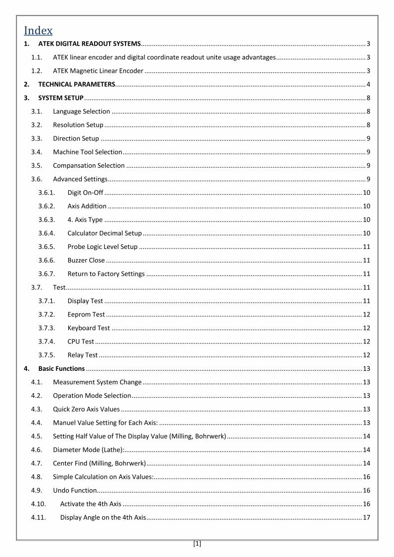
5.11. Simple Radius (Milling) This function is used to make accurate circle cutting on the work piece. The difference of the smooth function and

simple function is, in simple function you don’t give reference angle and finish angle, you only choice the needed one

from 8 quarter circle. The present positions evaluates as circle centre.

button is used to enter to the function. By button find the “Simple R.” writing. Press enter and find the plane

by buttons. Press enter to save. On the info screen after “TOOL PATH” writing, select one of the 8 tool ways.

After writing the number as 1 to 8 press enter to save. Enter the circle Radius. Press enter to save. Enter “Maximum

cutting distance and press enter. Determine if the tool diameter must be add or subtract.

If convex radius will be done as work piece 1 “R+ Tool” must be selected. If the radius will be done concave as work

piece 2 “R-Tool” must be selected. Press enter to save.

On info screen “POINT 1” will be written and on the axes the distances of the point 1 will be seen. Up to make zero

all axes the table is moved. And the Hole 1 is drilled. By button the point 2 distances will be seen. Up to make

zero all axes the table is moved. And hole 2 is drilled. By button the next point is passed. Up to drill all holes the

same operations will repeat. Please press button axis.

1 2 3 4

5 6 7 8

R+Tool

R-Tool

Tool Edge

Work piece 1

R + Tool must be used

Work piece 2

R – Tool must be used

[40]

Example: On XZ plane 50 mm diameter,

6 mm tool diameter and 12 mm max. cutting distance

simple radius as the picture direction;

→ → →

→ → →

→ →

→ →

→ →

→ →

→ → →

→ → →

→Point 2 values are seen. The table is moved up to zero the values. Drilling operation is done. The next point is

passed by button. The same operations are repeated for all points.

→After all points button is pressed to exit.

Find “Simple R” by

this button

Find XZ by this button

Select R-TOOL

(concave)

Move the table up to

make zero all axis values

on the screen and make

drilling.

50

mm

[41]

5.12. Linear Hole Patterns (Milling) Linear Hole Patterns Function is used to drill holes on the work piece as grid which includes requested line and

column number by user.

To make active linear hole patterns function the table is moved to first hole which will be drilled. button is

pressed and “Cos / F1” button is pressed. On the info screen there will be writing “LIN.ARRAY”. Press enter to make

active. By buttons the plane is selected. Press enter to save. Please select the “STEP” or “LENGTH” from two

options by buttons. Select the distance and press enter to save. Press enter to pass the other step. Press Sx

and enter the angle value. Press enter to save. Enter the column numbers. Press enter to save. Press Sy to enter the

line numbers. Press enter to save. You will see the distance for the first hole. It will be “0”. After drilling press

button you will see the distance for the 2nd hole. Move the table up to make zero the values and make drilling. Press

button to pass fallowing holes.and repeat the same opeartions. Press button to exit.

Example: XY plane,

Distance between column: 50mm

Line Distance: 40mm

Angle: 20°

Column quantity: 3

Line quantity: 2

To use linear hole patterns function by the givens;

→ → →

X

Y

50mm

40 mm 20°

First Hole

1. Eksen

2nd Axis

Step 1

Step 2

Length 1

Length 2

Angle

First Hole

1st Axis

[42]

→ → →

→ → →

→ → →

→ →

→ → →

→ →

→By button the coordinates are screened. All operations repeat for all points.

→ After drilling of all points you can exit by button.

Select “XY” plane by

these buttons

Select “ STEP”

by this button.

The first point is on reference

point so the value will be “0”.

Make drilling.

Move the table up to making zero the values

and make drilling.

[43]

5.13. Frame Hole Patterns (Milling) Frame hole patterns function is used fort o make a frame which created by the holes on the determined plane of the

work piece. The edge hole numbers must be determine by the user.

To active the function move the tablet o the first hole point. Press button and press “Sin / F2” button. You will

see “FRAME” writing on the screen. Press enter to open the function. Select the plane by the buttons. And

press enter button. The user has 2 options here. He can choice the distance between 2 holes as “STEP” or choice the

distance between the first hole and last hole as “length”. Use buttons for this choice. Enter the lenght / step

value and press enter to save. Enter the angle value. Press enter value. Press button and press Sx button again to

enter the clounm number. Press enter to save. Press Sy button to enter the line number. Enter the value and press

enter to save. Press button and see the distance value on the screen . For the first hole the value will be “0” .

After drilling press button and see the dşistance for the 2. Hole. Move the table to up to make zero the value

anddrill the 2. Hole. By . Button the next step is passed. These operations must be repeat for all holes and press

button to exit.

Example: On XY Plane,

Column Length: 60mm

Line Length: 90mm

Angle: 30°v

Column Number: 4

Line Number: 3

To use the function with the above data;

→ → →

→ → →

Select “XY” plane.

1st Axis

2nd Axis

Step 1

Step 2

Length 1

Length 2

Angle

First Hole

X First Hole

Y

90mm

60 mm

30°

X

[44]

→ → →

→ → →

→ →

→ → →

→ →

→ Pass to next hole. Repeat the operations for all holes.

→Press button to exit after all holes are drilled.

Select

“LENGTH”

It is the first hole so the

values are “0”.

Move the table up ro make “0” all values

[45]

5.14. Rectangular Pocket (Milling) When a rectangular hole is need on the work piece this function is used. It is good for a quality rectangular hole and

a better working time. The reference point is centre of the rectangular hole.

To use the function, press “Cos/F1” button. After pressing Sx button enter the tool diameter. Press enter to save. If

the tool is with Radius press “1” button to see “L-1” on the screen. If there is not Radius, press “0” to see “L-0” on

the screen. Press button to pass next step. Press Sx button and enter the distance of the X axis to the reference

point. Press enter to save. Press Sy and enter the distance of reference point to Y axis. Press enter to save. Press

button and Sx button and enter the length of X axis. Press enter to save. Press Sy button and enter the length of Y

axis and press enter to save. Press button to screen the moving distances. The table is moved up to making zero

the values. Press button and repeat the same operations for the other points. Press button to exit.

Example: Tool diameter: 8mm, no radius

Start point distance to X axis: 110 mm

Start point distance to Y axis: 90 mm

Rectangular Pocket X axis dimension: 100mm

Rectangular Pocket Y axis dimension: 80mm

Finish Depth: 3mm

To use rectangular pocket function with these data;

→ → → →

X

Y

0 110 mm

90 mm 80 mm

100 mm

See L-0 by pressing “0”

button because no

radius on insert tools.

X

Y

X

Y

0 Distance of centre to

X axis

Distance of

centre to Y axis. Y

X

[46]

→→ →

→ →

→ →

→ → →

→ →

→ →

Move the table up to make zero all

values and make drilling.

Move the table up to

make zero all values.

Next step is passed by this

button

After the operation press button

to exit.


www.ali5.ir

[47]

5.15. Work Piece Angle Measuring (Milling) By angle measuring function it is possible to measure the work piece angle.

For measuring the tool edge is moved to “Point 1” position. Then press button to enter the function. By

buttons select the axes which will be measure and press enter to save. When the tool edge moved to Point 2 on the

upper line there is written the angle. On the second line degree.minute.second values are screened by button

you can exit.

Example: To find the angle of the work piece as the left side;

→ →

→ → →

Axis 1

Axis 2

Point 1

Point 2

Açı

Work piece

X

Y

Point 1

Point 2

Angle?

Workpiece

Move the tool edge to

point 1.

Select “XY” plane by

these buttons.

Move the tool edge to

Point 2

See the angle as 29.998°.

[48]

5.16. Touch Probe (Milling, Bohrwerk) To ADR 10 series digital coordinate readout displays touch probe can be provided. When the contact probe contacts

to metal work piece the probe leds sign and probe menu is entered. By touch probe it is possible to make axis zero /

setting half value of the axis value, find center, measurement functions. Touch probe function can be opened by

pressing 10 times to x button on calculator and it is closed as the same way.

5.16.1. Zero the Axis / Setting Half Value of the Display Value

When the contact probe is contacted with the work piece find the “ZERO” selection by buttons. Press axis

selection button. When you cut the contact it zeros the axis and exit from the function automatically. Setting half

value of the display value, when you are on “ZERO” menu, select the axis and press “1/2” button.

Example: For setting half value of the Y axis value;

→ →

→ → →

→

X

Y

Find

“ZERO”

X

Y

X

Y


www.ali5.ir

[49]

5.16.2. Find Center

To find the work piece centre by contact probe, probe is contacted to first reference point of work piece on X axis

and when the menu is opened find the “CENTRE FND” option by buttons and press enter to open the

function. The probe uncontact to work piece and it is contacted to 2nd reference point on X axis and probe

uncontact. The first reference point of Y axis is contacted and uncontacted. Then the probe is contacted to 2nd

reference point and uncontact. After seeing “OK” writing on the screen press enter to see the distance to work piece

centre.

Example: To find the centre of the work piece by probe as below;

→

→ →

→

→

→

Contact the probe to

reference point 1

Find “CENTRE

FND”

Contact the

probe to

reference

point 2


reference point 3

X

Y

5mm 15mm

3mm

9mm

1 2

4

3

4,5mm

10mm


reference point 4

[50]

→ →

When the work pieces are moved up to make zero all axes you will find the work piece centre.

5.16.3. Measurement

To measure with contact probe when the probe is contacted to the work piece on the opened menu find

“MEASURE“ section by buttons and press enter to select. Probe must be contacted to Point 1.

On the opened function menu, the measure effect of probe is adjusted. If the measure of the work piece will be

taken as in the Picture 1 press “1” button and see “+DIAMETER” writing on the screen. If the measure of the work

piece will be taken as Picture 2 press “0” button and see “-DIAMETER” writing on the screen. Press “Sx” button and

enter probe diameter and press enter to save. Press button to see “POINT 1” writing. Press button of the axis

selection. When you uncontact the probe device, save Point 1. When you contact Point 2 the length will be deal to

user.

Example:

→ →

5 mm

Lenght?

As the left side picture to find inner dimesions of Y

axis

First contact Position;

X: 26.110 Y: 61.200 Z: 0.000 )

Point 1

Find

“MEASURE”

Şekil 1 Şekil 2

Point 1 Point 1 Point2 Point2

Probe diameter

[51]

→ →

→

→ → →

→

→

The length is calculated as 75 mm. Please press button to exit.

Point2

[52]

5.17. Tool Diameter Compansation (Milling) Tool diameter compensation is used to prevent the machining errors because of the tool diameter effects.

As example the 1st work piece wants to be machined. If you consider only a and b dimensions, because of the tool

effect the work piece will be machines wrongly. It is also important which work piece will be machined on which

side.

For Tool Diameter Compansation function moves the tool edge to the start point which the machining will be

started. And Tan / F3 button is pressed. On work piece the machining side must be selected by numeric buttons. By

button the next stepped is passed. Enter tool diameter. The table is moved up to seen the values of the real

dimensions of the work piece.

Example:

Move the tool to start point;

→ →

→

→

1 2 3

4 6

7 8 9

6

8

2

4

9

1

7

3

100 mm

Tool Diameter : 8mm

To machine the workpiece as the left picture;

Press “6” ( machining

direction of the workpiece)

The work piece will be machined up to

the X axis values are 100.000.

1 2 3

Φ Tool Diameter

Φ Tool Diameter

a

b

[53]

5.18. Tool Storeroom (Lathe) While machining the different work piece or different surfaces of the work piece, the different machine tools may be

needed. So you will need to change the machine tools. ADR10 digital coordinate readout has 1000 pcs tool

memories. By this way you don’t need to get zero point for each tool changing.

The tool must be open to use this function. To open the tool button must be pressed 10 times to open the too.

The registration of the tools can be made by automatically or manuel. For automatic registration please press

button and “Tool” button. The memory number must be set. On the zero point of X axis “Sx” button is pressed. On

the Y axis “Sy” button is pressed accordingly.

For manuel setting of tool memory “Tool” button is pressed and “Zero” button is pressed accordingly. Then the

memory number is set and “enter”. Sx button is pressed and X axis length is entered. Sy button is pressed and Y axis

length is entered button is pressed. You can exit by button. To make easier generally “0” is used for memory

number. For reference number of the tool dimensions “0” can be used for easy.

Example:

Tool Memory Setting First Way (Automatically):

10 x → →

Y1 Y2

X1 X2

Tool1 Tool 2

To memory; 2 different tool and to set

tool1 as reference and tool2 as

selection as left drawing

10 mm 12mm

3mm 5mm

Tool 1 Tool 2


www.ali5.ir

[54]

→ →

→ → →

→ → →

→ →

→ →

Tool Memory Setting Second Way ( Manuel): Move Y axis to zero point.

10 x → →

Determine X

axis as

referance

point.

Move Y axis to

zero point.

Install

2nd tool

Move X axis to

zero point.

Move Y axis to

zero point.

[55]

→

→ →

Selection of used tool and reference tool:

→ →

→ →

→

[56]

5.19. Taper Angle Measurement (Lathe) This function is designed for Lathe Machines to measure the Taper Object Hill Angle.

To taper object angle measure the tool edge moved to reference point and button is pressed. Then move the

tool edge to 2nd reference point and press enter. On X axis 2α angle and on Y axis α angle is seen.

Example: To measure the angle of taper work piece which connected to the lathe;

→ →

→ → →

α = 36,746 ° 2α = 73,492°

α

2α

α

Point 1 Point 2

Tool moves to 1st

reference point.

Tool moves to 2nd

reference point.

[57]

5.20. Digital Filter (Vibration Filter) In some applications because of vibration or scale the values of the display can be always change. For example in

grinding application because of the grinding machine vibration the values of the DRO display can be always change.

It disturbs the user. So we have added vibration filter function to the device. By this function renewing ratio of the

display is delayed and it makes easy usage for user. This delay never caused the position errors. The values are not

error, they are always correct position values. To change the display renewing ratio “EDM” button is pressed. Then

the renew time is set and “enter” is pressed to save the value. If the screen type is selected as “erosion” type, please

use “tool” button instead of “EDM” button to enter the function. The renew time must be between 10ms and 500

ms. The vibration decreases by the value. To exit, please press button.

Example: To make 100 ms the renew time of the screen;

→ →

→ → →

[58]

5.21. Inclined Z Axis Machining (Milling) This function is used to make inclined on the Z axis. This function is made on XZ or YZ plane.

The tool edge is moved to start point and press “Sin / F2” button and by buttons and the plane is selected.

Press enter to save. Enter angle (α) and press enter to save. Enter Z axis step distance (ΔZ) and press enter. If the

step distance is upper side save it possitive or if it is down side save it as negative. When you press button you

will see the firsyt point coordinates on the screen. If you select “YZ” plane the coordinates of X and Z axis will be

changed or İf you select XZ plane Y and Z axis coordinaates will be changed. Move the table up to make zero the axis

values. Press button for following steps.

tgA

ZIX

=)( ZxIIZ =)(

tgA

ZX

=

I: Step Number

ΔX: X Axis Step Distance

ΔZ: Z Axis Step Distance

* Inclined Z axis machining function is used as 4 different way. Before useing the function enter the “α“ value as

angle value.

YZ Plane XZ Plane

1 X/Y

Z Z

ΔX

ΔZ

X/Y

α α

2

X/Y

Z

α X/Y

Z

α

3 4

Z(I)

X(I)

[59]

Example:

→ → →

→

→

→

XZ Plane

30 °

To machine the workpiece as left Picture, on XZ

plane, 30° angle and 0,1 mm Z axis. 0,1mm Z axis

steps;

Select “XZ” Plane

by these buttons.

The workpiece is machined up to axis values are zero. By

button the next coordinate is screened. Up to machine whole

part these operations are repeated. Press button to exit.

[60]

5.22. EDM Depth Control Function (Erosion) This function is used for depth control on the erosion machines the work piece which will be machined Z axis. To

enter of the offset values is also possible to compensation of the electrode errors. Also two different modes can be

adjusted. When “MODE 0” is adjusted relay will be on and it continues up to requested depth. Also the device will

warn you when the requested depth is received.

When the electrode contact with the work piece the axis values will be zero. Press EDM button to enter the function.

On info screen you will see “DEPTH” writing. Press Sx and enter the depth value. Press enter to save. By button

you will see “Offset” writing on the info screen. Press Sx and enter the error value which would be occurring by

electrode. Press enter to save. This value will be added to depth distance. Press button again and press 1 or 0

button to select operation mode and press enter to save. When you select Mode 0 the relays will be on up to

requested depth. If you select Mode 1 relays will start with the normal position and it will be on when the requested

depth is received. After mode selection please press enter to save. Enter the axis to use EDM relay. (1 – X Axis, 2 – Y

Axis, 3 – Z Axis, 4 – W Axis)

While operation the “Z” led will be sign. On X axis the value which will be continue without offset is seen and on Y

axis you will see the max depth value. On Z axis you will see the present value.

Description Pin Number Function

P1 1 Standard Open Pin C1 2 Common Edge P2 3 Standard Closed Pin C2 4 Screen

Example:

The workpiece wants to be machined up to

50 mm depth as the left side picture.

Because of the electrode abrasion the

dimension decrease 3 mm. The relay wants

to be changed the position when the

requested depth is received. To use this EDM

function to control the depth; (On X Axis)

Electrode

Workpiece 0

Z

Electrode

Workpiece

e

0

Z

[61]

→ →

→ →

→ →

→ →

→

It shows 3 mm deficient

so 3mm is added. If it

shows 3 mm over the

offset value will be

enter -3.

When 50 mm + 3 mm (Offset) depth value is received the relay

changes its position and digital readout warns the user both by

written and sounds. To exit press EDM button or enter or

button. If the Mode 0 would be used the function would be

exited automatically.

Electrode

Workpiece 0

Z

50

[62]

5.23. HOLD Function You can freeze the values open the requested axis. After freezing the axis value if you move the tablet he axis value

can continue with the new position of the table. Or it can continue with the frozen values.

To activate the function select the axis which will be frozen and press “HOLD” button. Press again “HOLD” button

and you can move the table. The axis will be continued with the last position value. If you exit by button if the

table position is changed the axis value continues with the new value.

Example: Hold function for Y axis;

→

→ →

→

Way 1: Way 2:

→ →

X

Y

40

40

X

Y

50

50

When the workpiece possition is changed;

X:50 Y:50

2 ways for exit

[63]

5.24. Data Transfer by RS – 232 Port There is RS – 232 port on ADR 10 digital readout. By this way the coordinate data can be followed by computer. It

transfers the same coordinate informations if the DRO has how many coordinates. RS-232 port can transfer the

values up to 15 meters far. (Baud rate: 57.600, Parity None, Stop Bit:1)

A : Position Information CR LF

For X axis, axis number is 0

For Y axis, axis number is 1

For Z axis, axis number is 2

For W axis, axis number is 3

Example: The signals of ADR10 3 axis DRO RS – 232 output port.

0: 26.610

1: 6638.425

2: -42.890

Axis

Number

Bracket

Position

Information

Carriage Return

Character

Line Feed

Character

[64]

ATEK ELEKTRONİK SENSÖR TEKNOLOJİLERİ SANAYİ VE TİCARET A.Ş.

Gebze OSB, 800. Sokak, No:814 Gebze/KOCAELİ/TURKEY

Tel: +90 262 673 76 00

Fax : +90 262 673 76 08

Web: www.ateksensor.com

E-Mail: [email protected]


www.ali5.ir

http://www.ateksensor.com/

mailto:[email protected]

atek adr 10 series - kanooneabzar.com

Documents