at01 vam uncertainty
TRANSCRIPT
8/3/2019 At01 VAM Uncertainty
http://slidepdf.com/reader/full/at01-vam-uncertainty 1/90
VAM Project 3.2.1
Development andHarmonisat ion ofMeasurementUncertainty Principles
Part (d): Protocol for
uncertainty evaluation f romvalidation data
V J Barwick and S L R Ellison
January 2000
LGC/VAM/1998/088
Version 5.1

8/3/2019 At01 VAM Uncertainty
http://slidepdf.com/reader/full/at01-vam-uncertainty 2/90
Protocol for uncertaint yevaluat ion f romvalidat ion data
V J BarwickS L R Ellison
January 2000
Report No: LGC/VAM/1998/088
Cont act Point :
Vicki Barwick
Tel: 020 8943 7421
Prepared by:
Vicki Barwick
The wor k described in t his report was supported undercontract with the Department of Trade and Industry aspart of the National Measurement Systems ValidAnalyti cal M easurement (VAM) Programm e
Milestone ref: 3.2.1dLGC/VAM/1998/088
© LGC (Teddington) Limited 2000

8/3/2019 At01 VAM Uncertainty
http://slidepdf.com/reader/full/at01-vam-uncertainty 3/90
Version 5.1
LGC/VAM/1998/088 Page i
Contents
1. Int roduct ion 1
2. St ructure of the guide 2
3. Ident if icat ion of sources of uncertainty 6
4. Quant if icat ion of uncertainty cont ribut ions 8
4.1 Precision study 9
4.1.1 Single typical sample 9
4.1.2 Range of samples covering the method scope 10
4.2 Trueness study 13
4.2.1 Estimating Rm
and u( Rm
) using a representative certified reference material 16
4.2.2 Estimating Rm
and u( Rm
) from a spiking study at a single concentration on a single matrix 16
4.2.3 Estimating Rm
and u( Rm
) by comparison with a standard method 19
4.2.4 Other methods for estimating Rm
and u( Rm
) 19
4.2.5 Estimating the contribut ion of Rm
to u( R) 21
4.2.6 Estimating Rs and u( Rs) from spiking studies 22
4.2.7 Estimating Rrep and u( Rrep) 23
4.2.8 Calculating R and u( R) 24
4.3 Evaluation of other sources of uncertainty 25
4.3.1 Calibration certificates and manufacturers’ specifications 25
4.3.2 Published data 25
4.3.3 Experimental studies 26
5. Calculat ion of combined standard and expanded uncertaint ies 30
5.1 Combined standard uncertainty 30
5.1.1 All sources of uncertainty are proportional to the analyte concentration 30
5.1.2 Some sources of uncertainty are independent of analyte concentration 30
5.2 Expanded uncertainty 31
6. Report ing uncertainty 33
6.1 Reporting expanded uncertainty 336.2 Reporting standard uncertainty 33
6.3 Documentation 33
Annex 1: Cause and Effect Analysis 34
Annex 2: Calculating standard uncertainties 36
Annex 3: Definitions 37
Annex 4: Worked examples 41
Annex 5: Proforma for documenting uncertainty 82
Annex 6: References 86

8/3/2019 At01 VAM Uncertainty
http://slidepdf.com/reader/full/at01-vam-uncertainty 4/90
Version 5.1
LGC/VAM/1998/088 Page 1
1. IntroductionIt is now widely recognised that the evaluation of the uncertainty associated with a result
is an essential part of any quantitative analysis. Without knowledge of the measurement
uncertainty†, the statement of an analytical result cannot be considered complete. The
“Guide to the Expression of Uncertainty in Measurement”[1]
published by the
International Organisation for Standardisation (ISO) establishes general rules for
evaluating and expressing uncertainty for a wide range of measurements. The ISO guide
has subsequently been interpreted for analytical chemistry by Eurachem.[2]
The
Eurachem guide sets out procedures for the evaluation of uncertainty in analytical
chemistry. The main stages in the process are identified as:
• specification - write down a clear statement of what is being measured, including
the full expression used to calculate the result;• identify uncertainty sources - produce a list of all the sources of uncertainty
associated with the method;
• quantify uncertainty components - measure or estimate the magnitude of the
uncertainty associated with each potential source of uncertainty identified;
• calculate total uncertainty - combine the individual uncertainty components,
following the appropriate rules, to give the combined standard uncertainty for
the method; apply the appropriate coverage factor to give the expanded
uncertainty.
This guide focuses on the second and third stages outlined above, and in particular gives
guidance on how uncertainty estimates can be obtained from method validation
experiments. The guide does not offer definitive guidance on the requirements for
method validation, for which other texts are available.[3]
Instead, it recognises that key
studies routinely undertaken for validation purposes, namely precision studies, trueness
studies and ruggedness tests, can if properly planned and executed, also provide much of
the data required to produce an estimate of measurement uncertainty. Figure 1 illustrates
the key stages in the uncertainty estimation process. The purpose of this guide is
therefore to give guidance on the planning of suitable experiments that will meet therequirements of both method validation and uncertainty estimation. The procedures
described are illustrated by worked examples.
†
An alphabetical list of definitions is contained in Annex 3. Each term is highlighted in bold upon its firstoccurrence in the main body of the text.
8/3/2019 At01 VAM Uncertainty
http://slidepdf.com/reader/full/at01-vam-uncertainty 5/90
Version 5.1
LGC/VAM/1998/088 Page 2
Identify sources of
uncertainty (3)
Plan and carry out
precision study (4.1)
Plan and carry out
trueness study (4.2)
Identify additional sources of
uncertainty and evaluate (4.3)
Combine individual uncertainty
estimates to give standard and
expanded uncertainties for themethod (5)
Report and document
the uncertainty (6)
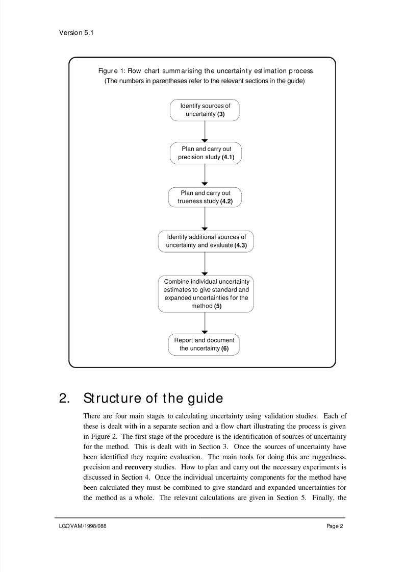
Figure 1: Flow chart summarising the uncertain ty est imat ion process
(The numbers in parentheses refer to the relevant sections in the guide)
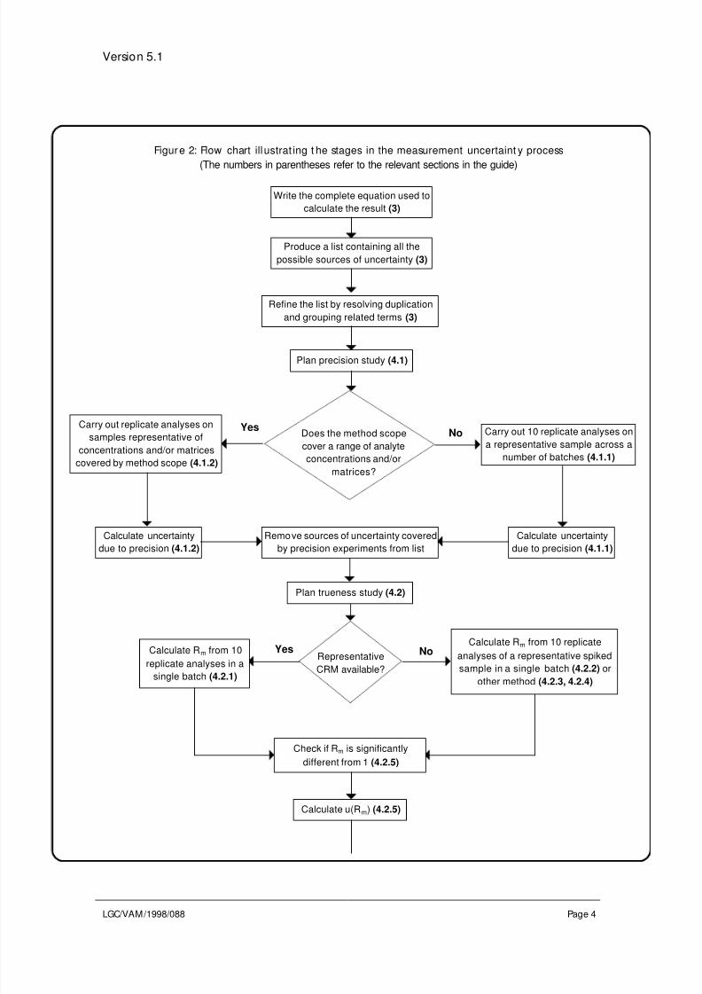
2. Structure of the guideThere are four main stages to calculating uncertainty using validation studies. Each of
these is dealt with in a separate section and a flow chart illustrating the process is given
in Figure 2. The first stage of the procedure is the identification of sources of uncertainty
for the method. This is dealt with in Section 3. Once the sources of uncertainty have
been identified they require evaluation. The main tools for doing this are ruggedness,
precision and recovery studies. How to plan and carry out the necessary experiments is
discussed in Section 4. Once the individual uncertainty components for the method have
been calculated they must be combined to give standard and expanded uncertainties for
the method as a whole. The relevant calculations are given in Section 5. Finally, the

8/3/2019 At01 VAM Uncertainty
http://slidepdf.com/reader/full/at01-vam-uncertainty 6/90
Version 5.1
LGC/VAM/1998/088 Page 3
standard and expanded uncertainties need to be reported and documented in an
appropriate way. This is discussed in Section 6. In addition to the sections mentioned
above, the guide also contains a number of annexes. Guidance on calculating standard
uncertainties from various sources of information, for example calibration certificates, is
given in Annex 2. Definitions are contained in Annex 3, worked examples are given in
Annex 4 and Annex 5 contains a proforma for documenting uncertainties.
8/3/2019 At01 VAM Uncertainty
http://slidepdf.com/reader/full/at01-vam-uncertainty 7/90
Version 5.1
LGC/VAM/1998/088 Page 4
Write the complete equation used to
calculate the result (3)
Produce a list containing all the
possible sources of uncertainty (3)
Refine the list by resolving duplication
and grouping related terms (3)
Plan precision study (4.1)
YesCarry out replicate analyses on
samples representative of
concentrations and/or matrices
covered by method scope (4.1.2)
Calculate uncertainty
due to precision (4.1.2)
Plan trueness study (4.2)
NoYesRepresentative
CRM available?
Calculate u(Rm) (4.2.5)
Does the method scope
cover a range of analyte
concentrations and/or
matrices?
No Carry out 10 replicate analyses on
a representative sample across a
number of batches (4.1.1)
Calculate uncertainty
due to precision (4.1.1)
Remove sources of uncertainty covered
by precision experiments from list
Check if Rm is significantly
different from 1 (4.2.5)
Calculate Rm from 10
replicate analyses in a
single batch (4.2.1)
Calculate Rm from 10 replicate
analyses of a representative spiked
sample in a single batch (4.2.2) or
other method (4.2.3, 4.2.4)
Figure 2: Flow chart ill ustrat ing t he stages in the measurement uncertaint y process
(The numbers in parentheses refer to the relevant sections in the guide)

8/3/2019 At01 VAM Uncertainty
http://slidepdf.com/reader/full/at01-vam-uncertainty 8/90
Version 5.1
LGC/VAM/1998/088 Page 5
Existing data
available?
Calculate uncertainty
(4.3.1, 4.3.2)
NoYes Carry out ruggedness
test (4.3.3.1)
No
Yes
Estimate uncertainty from
results of ruggedness test
(4.3.3.2)
Combine precision, recovery andadditional uncertainties to give
combined standard uncertainty (5.1)
Calculate uncertainty
(4.3.3.3)
Calculate the expanded
uncertainty (5.2)
Report and document
the uncertainty (6)
Identify sources of uncertainty not covered
by precision/trueness studies (4.3)
Does parameter have
a significant effect on
result? (4.3.3.1)
Figure 2 continued
Remove sources of uncertainty covered
by trueness study from list
No
Combine all recovery
uncertainties to give R and u(R)
(4.2.8)
Does the method scope
cover a range of analyte
concentrations and/or
matrices?
No
Yes Calculate Rrep and
u(Rrep) (4.2.7)Spiking study used
to estimate Rm?
YesCalculate Rs and u(Rs)
(4.2.6)
Use data from ruggedness
study/ carry out additional
experiments (4.3.3.3)

8/3/2019 At01 VAM Uncertainty
http://slidepdf.com/reader/full/at01-vam-uncertainty 9/90
Version 5.1
LGC/VAM/1998/088 Page 6
3. Ident if icat ion of sources of uncertaint yOne of the critical stages of any uncertainty study is the identification of all the possible
sources of uncertainty. The aim is to produce a list containing all the possible sources of
uncertainty for the method. At this stage it is not necessary to be concerned about the
quantification of the individual components; the aim is to be clear about what needs to be
considered in the uncertainty budget. The Eurachem Guide discusses the process of
identifying sources of uncertainty and a number of typical sources of uncertainty are
given, including:
• Sampling - where sampling forms part of the procedure, effects such as random
variations between different samples and any bias in the sampling procedure
need to be considered.
• Instrument bias - e.g., calibration of analytical balances.
• Reagent purity - e.g., the purity of reagents used to prepare calibration standards
will contribute to the uncertainty in the concentration of the standards.
• Measurement conditions - e.g., volumetric glassware may be used at
temperatures different from that at which it was calibrated.
• Sample effects - The recovery of an analyte from the sample matrix, or an
instrument response, may be affected by other components in the matrix. When
a spike is used to estimate recovery, the recovery of the analyte from the sample
may differ from the recovery of the spike, introducing an additional source of
uncertainty.
• Computational effects - e.g., using an inappropriate calibration model.
• Random effects - random effects contribute to the uncertainty associated with all
stages of a procedure and should be included in the list as a matter of course.
A simple approach to identifying the sources of uncertainty is as follows:
3.1 Write down the complete calculation involved in obtaining the result, including all
intermediate measurements. List the parameters involved.
3.2 Study the method, step by step, and identify any other factors acting on the result.
Add these to the list. For example, ambient conditions such as temperature and
pressure affect many results.
3.3 Consider factors which will affect the parameters identified in 3.1 and 3.2 and add
them to the list. Continue the process until the effects become too remote to be
worth consideration.
3.4 Resolve any duplicate entries in the list. Listing uncertainty contributions
separately for every input parameter will result in duplications in the list. Three
cases arise and the following rules should be applied to resolve duplication:
8/3/2019 At01 VAM Uncertainty
http://slidepdf.com/reader/full/at01-vam-uncertainty 10/90
Version 5.1
LGC/VAM/1998/088 Page 7
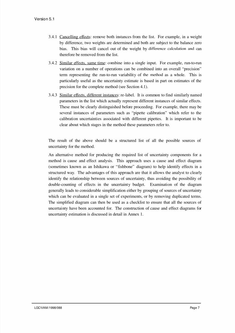
3.4.1 Cancelling effects: remove both instances from the list. For example, in a weight
by difference, two weights are determined and both are subject to the balance zero
bias. This bias will cancel out of the weight by difference calculation and can
therefore be removed from the list.
3.4.2 Similar effects, same time: combine into a single input. For example, run-to-run
variation on a number of operations can be combined into an overall “precision”
term representing the run-to-run variability of the method as a whole. This is
particularly useful as the uncertainty estimate is based in part on estimates of the
precision for the complete method (see Section 4.1).
3.4.3 Similar effects, different instances: re-label. It is common to find similarly named
parameters in the list which actually represent different instances of similar effects.
These must be clearly distinguished before proceeding. For example, there may be
several instances of parameters such as “pipette calibration” which refer to the
calibration uncertainties associated with different pipettes. It is important to be
clear about which stages in the method these parameters refer to.
The result of the above should be a structured list of all the possible sources of
uncertainty for the method.
An alternative method for producing the required list of uncertainty components for a
method is cause and effect analysis. This approach uses a cause and effect diagram
(sometimes known as an Ishikawa or “fishbone” diagram) to help identify effects in a
structured way. The advantages of this approach are that it allows the analyst to clearly
identify the relationship between sources of uncertainty, thus avoiding the possibility of
double-counting of effects in the uncertainty budget. Examination of the diagram
generally leads to considerable simplification either by grouping of sources of uncertainty
which can be evaluated in a single set of experiments, or by removing duplicated terms.
The simplified diagram can then be used as a checklist to ensure that all the sources of
uncertainty have been accounted for. The construction of cause and effect diagrams for
uncertainty estimation is discussed in detail in Annex 1.

8/3/2019 At01 VAM Uncertainty
http://slidepdf.com/reader/full/at01-vam-uncertainty 11/90
Version 5.1
LGC/VAM/1998/088 Page 8
4. Quant if icat ion of uncertaintycontributionsThe next stage in the process is the planning of experiments which will provide the
information required to obtain an estimate of the combined uncertainty for the method.
Initially, two sets of experiments are carried out - a precision study and a trueness study.
These experiments should be planned in such a way that as many of the sources of
uncertainty identified in the list obtained in Section 3 as possible are covered. The
contributions covered by the precision and trueness studies can then be removed from the
list. Those parameters not adequately covered by these experiments are evaluated
separately. This section discusses the types of experiments required and gives details of
how the data obtained are used to calculate uncertainty. The results from such studies
will also be required as part of a validation exercise. However, the experiments givenhere do not necessarily form a complete validation study and further experiments may be
required, for example, linearity or detection limit studies.[3]
The stages in the quantification of measurement uncertainty are as follows:
• precision study;
• trueness study;
• identification of other uncertainty contributions not adequately covered by the
precision and trueness studies;
• evaluation of the other uncertainty contributions.
Each of these stages is discussed below. The simplest case is the estimation of precision
from the replicate analysis of a single typical sample and the estimation of trueness from
the analysis of a representative certified reference material (CRM). The appropriate
experiments are described in 4.1.1 and 4.2.1 below. However, for many methods the
situation will be more complex than this and the procedures for dealing with a number of
common situations are outlined in Sections 4.1, 4.2 and 4.3.
When deciding which experiments are appropriate for the evaluation of a particular
method, it is important to keep in mind one of the key principles of method validation and
uncertainty estimation: the studies must be representative of normal operation of the
method. That is the studies must cover the complete method, a representative range of
sample matrices and a representative range of analyte concentrations. In other words,
they must cover the full scope of the method.
8/3/2019 At01 VAM Uncertainty
http://slidepdf.com/reader/full/at01-vam-uncertainty 12/90
Version 5.1
LGC/VAM/1998/088 Page 9
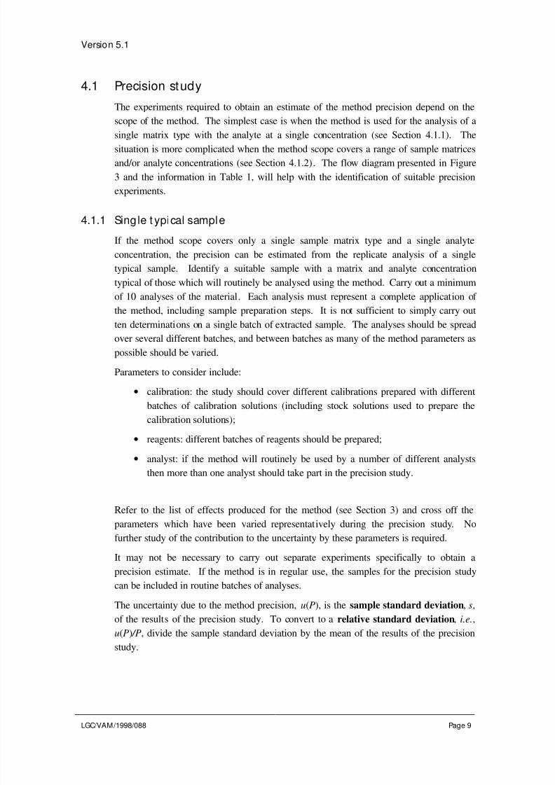
4.1 Precision study
The experiments required to obtain an estimate of the method precision depend on the
scope of the method. The simplest case is when the method is used for the analysis of a
single matrix type with the analyte at a single concentration (see Section 4.1.1). Thesituation is more complicated when the method scope covers a range of sample matrices
and/or analyte concentrations (see Section 4.1.2). The flow diagram presented in Figure
3 and the information in Table 1, will help with the identification of suitable precision
experiments.
4.1.1 Single t ypical sample
If the method scope covers only a single sample matrix type and a single analyte
concentration, the precision can be estimated from the replicate analysis of a single
typical sample. Identify a suitable sample with a matrix and analyte concentration
typical of those which will routinely be analysed using the method. Carry out a minimum
of 10 analyses of the material. Each analysis must represent a complete application of
the method, including sample preparation steps. It is not sufficient to simply carry out
ten determinations on a single batch of extracted sample. The analyses should be spread
over several different batches, and between batches as many of the method parameters as
possible should be varied.
Parameters to consider include:
• calibration: the study should cover different calibrations prepared with different
batches of calibration solutions (including stock solutions used to prepare the
calibration solutions);
• reagents: different batches of reagents should be prepared;
• analyst: if the method will routinely be used by a number of different analysts
then more than one analyst should take part in the precision study.
Refer to the list of effects produced for the method (see Section 3) and cross off the
parameters which have been varied representatively during the precision study. No
further study of the contribution to the uncertainty by these parameters is required.
It may not be necessary to carry out separate experiments specifically to obtain a
precision estimate. If the method is in regular use, the samples for the precision study
can be included in routine batches of analyses.
The uncertainty due to the method precision, u(P), is the sample standard deviation, s,
of the results of the precision study. To convert to a relative standard deviation, i.e.,
u(P) /P, divide the sample standard deviation by the mean of the results of the precision
study.

8/3/2019 At01 VAM Uncertainty
http://slidepdf.com/reader/full/at01-vam-uncertainty 13/90
Version 5.1
LGC/VAM/1998/088 Page 10
4.1.2 Range of samples covering the method scope
In many cases a method will be used for the determination of an analyte at a range of
concentrations in a range of matrices. In such cases the precision study must consider a
range of representative samples. It may be possible to use a single uncertainty estimate
that covers all the sample types specified in the method scope, if there is evidence to
suggest that the uncertainties are comparable. However, it may be found that different
sample matrices and/or analyte concentrations behave differently so in some cases
separate uncertainty estimates will be required.
4.1.2.1 Single analyt e concentration, range of sample mat rices
Identify samples representative of each of the matrices covered by the method scope. If
the method has a broad scope it may not be practical to analyse, in replicate, a sample of
each matrix type. In such cases it is up to the analyst to decide on the appropriate
number and type of samples to be analysed. Analyse each sample in replicate. Ideally,
at least 10 replicate analyses should be carried out for each sample. However, if a large
number of matrices are being investigated this may be impractical, depending on the
method. A minimum of four replicates per sample is therefore recommended. The
replicates for each sample should be spread across different batches of analyses (see
Section 4.1.1).
Calculate the standard deviation of the results obtained for each sample. If the standard
deviations are not significantly different, they can be pooled to give a single estimate of
precision which can be applied to all the matrices covered by the precision study (seeEq. 4.1). However, if one or more of the matrices produce standard deviations which are
very different, it will be necessary to calculate separate uncertainty budgets for these
matrices.
Deciding whether or not there is a “significant” difference between the standard
deviations obtained for each sample is ultimately up to the analyst. Statistical tests can
be used but their value depends very much on the number of results available for each
sample. If 10 or more replicates have been made for each sample, the standard
deviations can be compared using F-tests[4]
. If a smaller number of results are available
for each sample then it is more appropriate for the analyst to decide whether to pool the
standard deviations or not. In making this decision, the contribution of the uncertainty
due to precision to the combined uncertainty for the method as whole should be borne in
mind. If the precision uncertainty is a dominant contribution it follows that the estimate
used will have a significant effect on the combined uncertainty. Therefore, pooling
precision estimates which cover a wide range of values may lead to a substantial
underestimate in the combined uncertainty for some matrices and an overestimate for
others. If, however, the precision uncertainty is not a major component of the combined
uncertainty, its value will have less of an impact. Therefore, pooling the precision
estimates should not lead to a significant over or underestimate of the combined
uncertainty for a particular matrix.
8/3/2019 At01 VAM Uncertainty
http://slidepdf.com/reader/full/at01-vam-uncertainty 14/90
Version 5.1
LGC/VAM/1998/088 Page 11
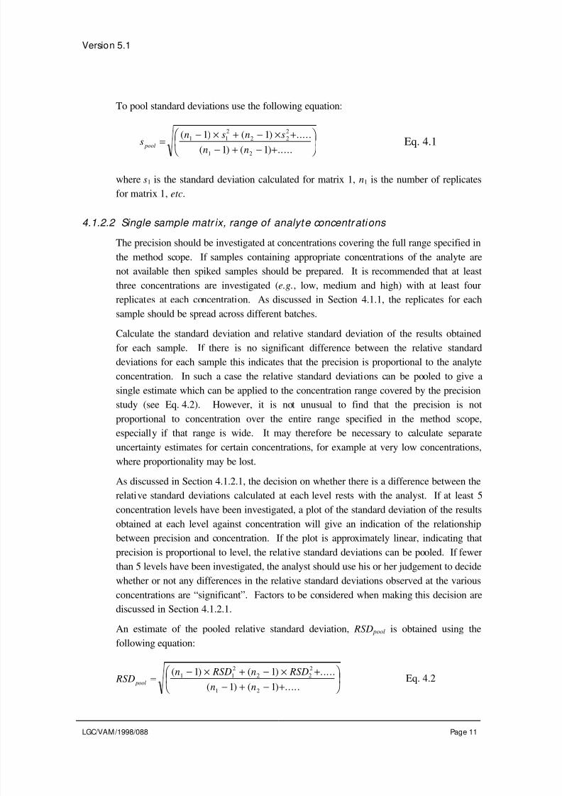
To pool standard deviations use the following equation:
s n s n sn n
pool = − × + − × +− + − + ( ) ( ) .....( ) ( ) .....
1
2
2
2
1 2
1 2
1 11 1
Eq. 4.1
where s1 is the standard deviation calculated for matrix 1, n1 is the number of replicates
for matrix 1, etc.
4.1.2.2 Single sample matr ix, range of analyte concentrations
The precision should be investigated at concentrations covering the full range specified in
the method scope. If samples containing appropriate concentrations of the analyte are
not available then spiked samples should be prepared. It is recommended that at least
three concentrations are investigated (e.g., low, medium and high) with at least four
replicates at each concentration. As discussed in Section 4.1.1, the replicates for each
sample should be spread across different batches.
Calculate the standard deviation and relative standard deviation of the results obtained
for each sample. If there is no significant difference between the relative standard
deviations for each sample this indicates that the precision is proportional to the analyte
concentration. In such a case the relative standard deviations can be pooled to give a
single estimate which can be applied to the concentration range covered by the precision
study (see Eq. 4.2). However, it is not unusual to find that the precision is not
proportional to concentration over the entire range specified in the method scope,especially if that range is wide. It may therefore be necessary to calculate separate
uncertainty estimates for certain concentrations, for example at very low concentrations,
where proportionality may be lost.
As discussed in Section 4.1.2.1, the decision on whether there is a difference between the
relative standard deviations calculated at each level rests with the analyst. If at least 5
concentration levels have been investigated, a plot of the standard deviation of the results
obtained at each level against concentration will give an indication of the relationship
between precision and concentration. If the plot is approximately linear, indicating that
precision is proportional to level, the relative standard deviations can be pooled. If fewer
than 5 levels have been investigated, the analyst should use his or her judgement to decide
whether or not any differences in the relative standard deviations observed at the various
concentrations are “significant”. Factors to be considered when making this decision are
discussed in Section 4.1.2.1.
An estimate of the pooled relative standard deviation, RSD pool is obtained using the
following equation:
RSDn RSD n RSD
n n pool
=− × + − × +
− + − +
( ) ( ) .....
( ) ( ) .....
1 1
2
2 2
2
1 2
1 1
1 1Eq. 4.2
8/3/2019 At01 VAM Uncertainty
http://slidepdf.com/reader/full/at01-vam-uncertainty 15/90
Version 5.1
LGC/VAM/1998/088 Page 12
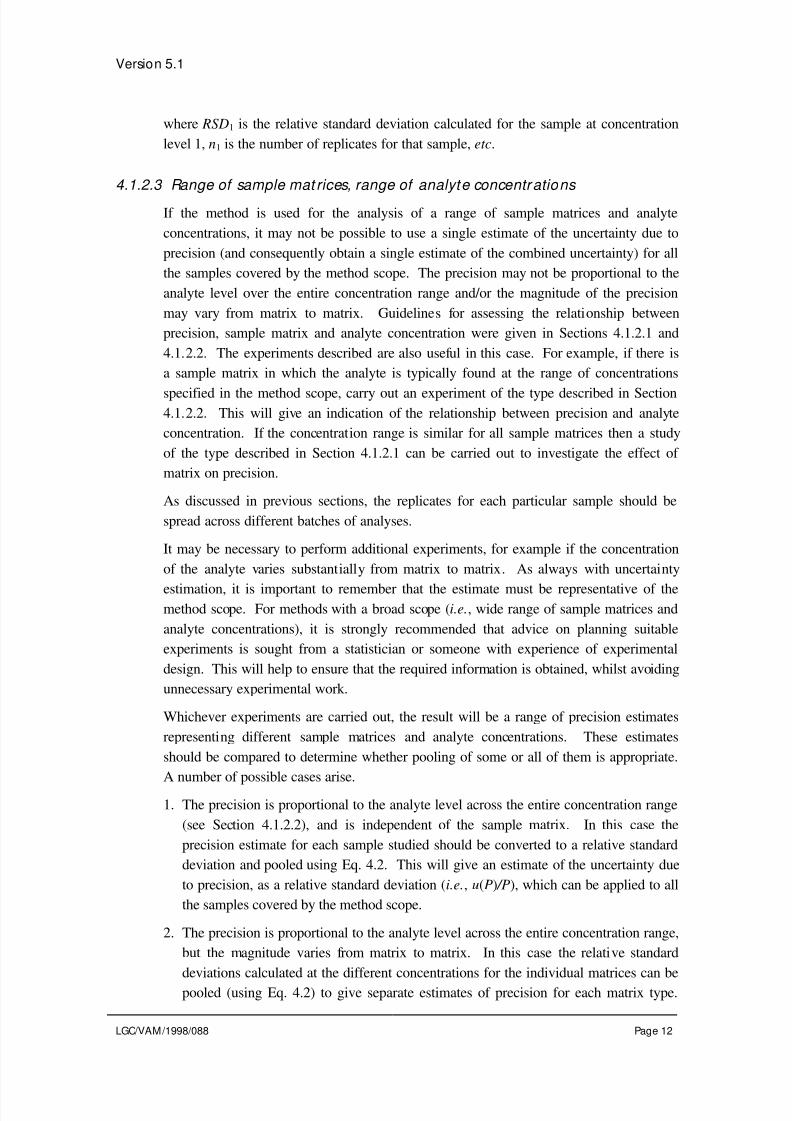
where RSD1 is the relative standard deviation calculated for the sample at concentration
level 1, n1 is the number of replicates for that sample, etc.
4.1.2.3 Range of sample mat rices, range of analyte concentrations
If the method is used for the analysis of a range of sample matrices and analyte
concentrations, it may not be possible to use a single estimate of the uncertainty due to
precision (and consequently obtain a single estimate of the combined uncertainty) for all
the samples covered by the method scope. The precision may not be proportional to the
analyte level over the entire concentration range and/or the magnitude of the precision
may vary from matrix to matrix. Guidelines for assessing the relationship between
precision, sample matrix and analyte concentration were given in Sections 4.1.2.1 and
4.1.2.2. The experiments described are also useful in this case. For example, if there is
a sample matrix in which the analyte is typically found at the range of concentrations
specified in the method scope, carry out an experiment of the type described in Section4.1.2.2. This will give an indication of the relationship between precision and analyte
concentration. If the concentration range is similar for all sample matrices then a study
of the type described in Section 4.1.2.1 can be carried out to investigate the effect of
matrix on precision.
As discussed in previous sections, the replicates for each particular sample should be
spread across different batches of analyses.
It may be necessary to perform additional experiments, for example if the concentration
of the analyte varies substantially from matrix to matrix. As always with uncertainty
estimation, it is important to remember that the estimate must be representative of themethod scope. For methods with a broad scope (i.e., wide range of sample matrices and
analyte concentrations), it is strongly recommended that advice on planning suitable
experiments is sought from a statistician or someone with experience of experimental
design. This will help to ensure that the required information is obtained, whilst avoiding
unnecessary experimental work.
Whichever experiments are carried out, the result will be a range of precision estimates
representing different sample matrices and analyte concentrations. These estimates
should be compared to determine whether pooling of some or all of them is appropriate.
A number of possible cases arise.
1. The precision is proportional to the analyte level across the entire concentration range
(see Section 4.1.2.2), and is independent of the sample matrix. In this case the
precision estimate for each sample studied should be converted to a relative standard
deviation and pooled using Eq. 4.2. This will give an estimate of the uncertainty due
to precision, as a relative standard deviation (i.e., u(P) /P), which can be applied to all
the samples covered by the method scope.
2. The precision is proportional to the analyte level across the entire concentration range,
but the magnitude varies from matrix to matrix. In this case the relative standard
deviations calculated at the different concentrations for the individual matrices can be
pooled (using Eq. 4.2) to give separate estimates of precision for each matrix type.

8/3/2019 At01 VAM Uncertainty
http://slidepdf.com/reader/full/at01-vam-uncertainty 16/90
Version 5.1
LGC/VAM/1998/088 Page 13
This will in turn lead to separate estimates of the combined uncertainty for each
matrix.
3. The precision is not proportional to the analyte level over the entire concentration
range. The experimental studies may show that the precision is proportional to theconcentration over only a limited concentration range, or not at all. In addition, this
may vary from matrix to matrix. In such cases it may be possible to pool some of the
precision estimates to give estimates of u(P) for particular groups of sample matrices
and/or concentration ranges. For example, for a particular method it was observed
that at low concentrations the standard deviation was similar for a range of sample
matrices and remained fixed over a narrow concentration range. This indicates that
the precision is independent of both the matrix and analyte level for the concentration
range studied. In such a case the standard deviations observed for each sample can be
pooled using Eq. 4.1 to give a single estimate of precision that can be applied to that
particular group of samples.
In summary, when the method scope covers a range of sample matrices and analyte
concentrations, the aim should be to pool precision estimates were appropriate. If the
precision is proportional to the concentration of the analyte the precision estimates should
be pooled as relative standard deviations using Eq. 4.2. If the precision is found to be
independent of the analyte concentration then the estimates should be pooled as standard
deviations using Eq. 4.2. As discussed in Sections 4.1.2.1 and 4.1.2.2, the decision on
whether or not it is appropriate to pool precision estimates rests with the analyst. Factors
to be considered and suitable statistical tests are given in these sections.
4.2 Trueness study
In this protocol, trueness is estimated in terms of overall recovery, i.e., the ratio of the
observed value to the expected value. The closer the ratio is to 1, the smaller the bias in
the method. Recovery can be evaluated in a number of ways, for example the analysis of
certified reference materials (CRMs) or spiked samples. The experiments required to
evaluate recovery and its uncertainty will depend on the scope of the method and the
availability, or otherwise, of suitable CRMs. The recovery for a particular sample, R,
can be considered as comprising three components:
• Rm
is an estimate of the mean method recovery obtained from, for example, the
analysis of a CRM or a spiked sample. The uncertainty in Rmis composed of
the uncertainty in the reference value (e.g., the uncertainty in the certified value
of a reference material) and the uncertainty in the observed value (e.g., the
standard deviation of the mean of replicate analyses). The contribution of Rmto
the overall uncertainty of the method depends on whether it is significantly
different from 1, and if so, whether a correction is applied.

8/3/2019 At01 VAM Uncertainty
http://slidepdf.com/reader/full/at01-vam-uncertainty 17/90
Version 5.1
LGC/VAM/1998/088 Page 14
• Rs is a correction factor to take account of differences in the recovery for a
particular sample compared to the recovery observed for the material used to
estimate Rm .
• Rrep is a correction factor to take account of the fact that a spiked sample maybehave differently to a real sample with incurred analyte.
These three elements are combined multiplicatively to give an estimate of the recovery for
a particular sample, i.e., R R R Rm s rep= × × . It therefore follows that the uncertainty in
R, u( R), will have contributions from u Rm
( ) , u( Rs) and u( Rrep). How each of these
components and their uncertainties are evaluated will depend on the method scope and the
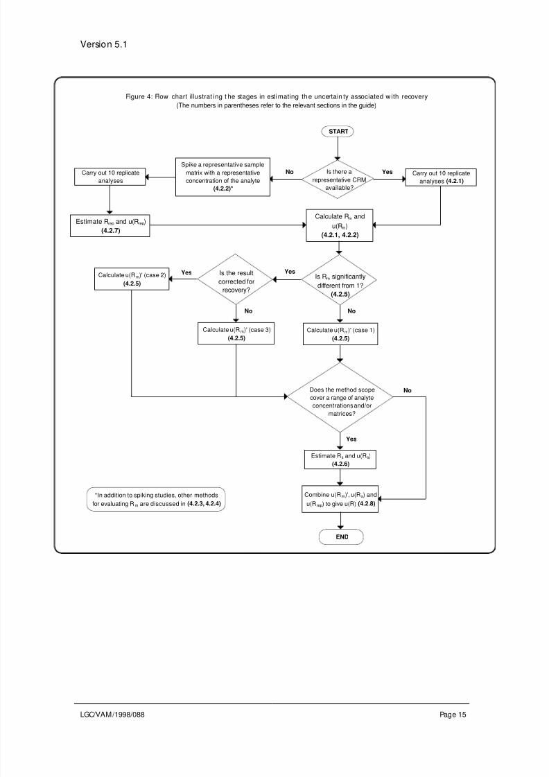
availability of reference materials. The various options are summarised in Figure 4 and
Table 2.
Approaches to estimating recovery, together with worked examples, are discussed inmore detail elsewhere.
[5, 6]
8/3/2019 At01 VAM Uncertainty
http://slidepdf.com/reader/full/at01-vam-uncertainty 18/90
Version 5.1
LGC/VAM/1998/088 Page 15
Calculate Rm and
u(Rm)
(4.2.1, 4.2.2)
START
Is there a
representative CRM
available?
YesNo Carry out 10 replicate
analyses (4.2.1)
Is Rm significantly
different from 1?
(4.2.5)
No
Yes
No
Yes
Calculate u(Rm)' (case 1)
(4.2.5)
Calculate u(Rm)' (case 3)
(4.2.5)
Calculate u(Rm)' (case 2)
(4.2.5)
Does the method scope
cover a range of analyte
concentrations and/ormatrices?
No
END
Yes
Spike a representative sample
matrix with a representative
concentration of the analyte
(4.2.2)*
Carry out 10 replicate
analyses
Estimate Rrep and u(Rrep)
(4.2.7)
Is the resultcorrected for
recovery?
Estimate Rs and u(Rs)
(4.2.6)
Combine u(Rm)', u(Rs) and
u(Rrep) to give u(R) (4.2.8)
*In addition to spiking studies, other methods
for evaluating Rm are discussed in (4.2.3, 4.2.4)
Figure 4: Flow chart illustrat ing t he stages in esti mating th e uncertain ty associated w ith recovery
(The numbers in parentheses refer to the relevant sections in the guide)

8/3/2019 At01 VAM Uncertainty
http://slidepdf.com/reader/full/at01-vam-uncertainty 19/90
Version 5.1
LGC/VAM/1998/088 Page 16
4.2.1 Estimating R m and u( R m ) using a representat ive cert if ied reference
material
Identify a certified reference material with a matrix and analyte concentrationrepresentative of those which will routinely be analysed using the method. Analyse at
least 10 portions of the reference material in a single batch.‡
Each portion must be taken
through the entire analytical procedure. Calculate the mean recovery, Rm
, as follows:
RC
C m
obs
CRM
= Eq. 4.3
where C obs
is the mean of the replicate analyses of the CRM and C CRM is the certified
value for the CRM.
Calculate the uncertainty in the recovery, u Rm( ) , using:
u R Rs
n C
u C
C m m
obs
obs
CRM
CRM
( )( )
= ××
+
2
2
2
Eq. 4.4
where sobs is the standard deviation of the results from the replicate analyses of the CRM,
n is the number of replicates and u(C CRM ) is the standard uncertainty in the certified value
for the CRM. See Annex 2 for information on calculating standard uncertainties from
reference material certificates.
The above calculation provides an estimate of the mean method recovery and itsuncertainty. The contribution of recovery and its uncertainty to the combined uncertainty
for the method depends on whether the recovery is significantly different from 1, and if
so, whether or not a correction is made. Section 4.2.5 gives guidance on estimating the
contribution of recovery to the combined uncertainty.
4.2.2 Estimating R m and u( R m ) f rom a spiking study at a single
concentration on a single mat rix
If there is no appropriate CRM available then Rm
and u Rm
( ) can be estimated from a
spiking study, i.e., the addition of the analyte to a previously studied material. Thespiked sample should be prepared in such a way as to represent a test sample as closely
as possible. There are several approaches to this, depending on whether a “blank”
sample matrix, free from the analyte of interest is available.
‡
If it is impractical to carry out 10 analyses in a single batch, the replicates should be analysed in the minimumnumber of batches possible over a short period of time.
8/3/2019 At01 VAM Uncertainty
http://slidepdf.com/reader/full/at01-vam-uncertainty 20/90
Version 5.1
LGC/VAM/1998/088 Page 17
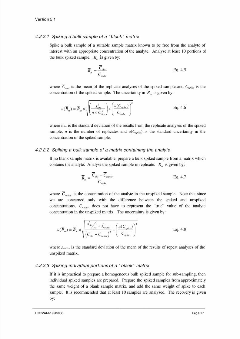
4.2.2.1 Spiking a bulk sample of a “ blank” matrix
Spike a bulk sample of a suitable sample matrix known to be free from the analyte of
interest with an appropriate concentration of the analyte. Analyse at least 10 portions of
the bulk spiked sample. Rm is given by:
RC
C m
obs
spike
= Eq. 4.5
where C obs
is the mean of the replicate analyses of the spiked sample and C spike is the
concentration of the spiked sample. The uncertainty in Rm
is given by:
u R Rs
n C
u C
C m m
obs
obs
spike
spike
( )( )
= ××
+
2
2
2
Eq. 4.6
where sobs is the standard deviation of the results from the replicate analyses of the spiked
sample, n is the number of replicates and u(C spike) is the standard uncertainty in the
concentration of the spiked sample.
4.2.2.2 Spiking a bulk sample of a matrix containing the analyte
If no blank sample matrix is available, prepare a bulk spiked sample from a matrix which
contains the analyte. Analyse the spiked sample in replicate. Rm
is given by:
RC C
C m
obs native
spike=
−Eq. 4.7
where C native
is the concentration of the analyte in the unspiked sample. Note that since
we are concerned only with the difference between the spiked and unspiked
concentrations, C native
does not have to represent the “true” value of the analyte
concentration in the unspiked matrix. The uncertainty is given by:
( )u R R
sn
s
C C
u C
C m m
obsnative
obs native
spike
spike
( )( )
= ×+
−+
22
2
2
Eq. 4.8
where snative is the standard deviation of the mean of the results of repeat analyses of the
unspiked matrix.
4.2.2.3 Spiking individual port ions of a “ blank” matrix
If it is impractical to prepare a homogeneous bulk spiked sample for sub-sampling, then
individual spiked samples are prepared. Prepare the spiked samples from approximately
the same weight of a blank sample matrix, and add the same weight of spike to each
sample. It is recommended that at least 10 samples are analysed. The recovery is given
by:

8/3/2019 At01 VAM Uncertainty
http://slidepdf.com/reader/full/at01-vam-uncertainty 21/90
Version 5.1
LGC/VAM/1998/088 Page 18
Rm
mm
obs
spike
= Eq. 4.9
where mobs is the mean weight of the spike recovered from the samples and mspike is theweight of the spike added to each sample. u R
m( ) is given by:
u R Rs
n m
u m
mm m
m
obs
spike
spike
obs( )( )
= ××
+
2
2
2
Eq. 4.10
where smobsis the standard deviation of the results obtained from the spiked samples, n is
the number of spiked samples analysed and u(mspike) is the uncertainty in the amount of
spike added to each sample.
4.2.2.4 Spiking indiv idual portions of a matrix containing the analyte
If the spiked samples are prepared from a sample matrix which contains the analyte the
situation is somewhat more complex. The recovery for each sample, Rm(i), is given by:
RC C
C m i
obs i native
spike i
( )
( )
( )
=−
Eq. 4.11
where C obs(i) is the concentration of the analyte observed for sample i and C spike(i) is the
concentration of the spike added to sample i.
The mean recovery, Rm , is given by:
Rn
C C
C m
obs i native
spike ii
n
=−
=∑1
1
( )
( )
Eq. 4.12
The uncertainty, u Rm
( ) , is given by:
( )
u Rn C
u C n C
u C
n
C C
C u C
m
spike i
obs i
spike ii
n
native
i
n
obs i native
spike i
spike i
i
n
( ) ( ) ( )
( )
( )
( )
( )
( )
( )
( )
2
2
1
2
2
1
2
2
1
1 1 1 1
1
= × ×
+
×
+ × − ×
==
=
∑∑
∑
Eq. 4.13
However, if the following conditions are met, Eq. 4.13 simplifies and Eq. 4.14 can be
used:
• u(C spike(i)) is much smaller than u(C obs(i)) and u(C native). This is often the case, as
spiking is generally achieved by adding an aliquot of a solution or a known
weight of the analyte. The uncertainties associated with such operations are
usually small compared to the uncertainties associated with the observation of the
amount of the analyte in a sample.
8/3/2019 At01 VAM Uncertainty
http://slidepdf.com/reader/full/at01-vam-uncertainty 22/90
Version 5.1
LGC/VAM/1998/088 Page 19
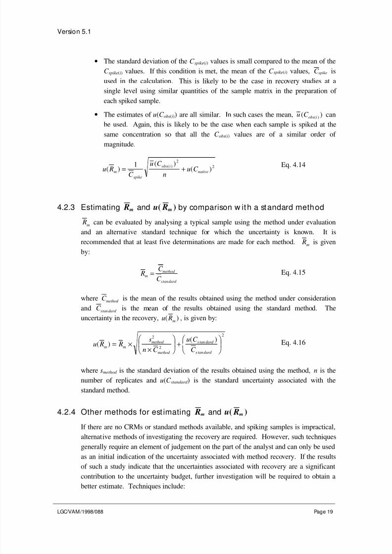
• The standard deviation of the C spike(i) values is small compared to the mean of the
C spike(i) values. If this condition is met, the mean of the C spike(i) values, C spike is
used in the calculation. This is likely to be the case in recovery studies at a
single level using similar quantities of the sample matrix in the preparation of
each spiked sample.
• The estimates of u(C obs(i)) are all similar. In such cases the mean, u C obs i( )( ) can
be used. Again, this is likely to be the case when each sample is spiked at the
same concentration so that all the C obs(i) values are of a similar order of
magnitude.
u RC
u C
nu C m
spike
obs i
native( )( )
( )( )= +
12
2 Eq. 4.14
4.2.3 Estimating R m and u( R m ) by comparison w ith a standard method
Rm
can be evaluated by analysing a typical sample using the method under evaluation
and an alternative standard technique for which the uncertainty is known. It is
recommended that at least five determinations are made for each method. Rm
is given
by:
RC
C m
method
s dard
=tan
Eq. 4.15
where C method
is the mean of the results obtained using the method under consideration
and C s dard tan
is the mean of the results obtained using the standard method. The
uncertainty in the recovery, u Rm
( ) , is given by:
u R Rs
n C
u C
C m m
method
method
s dard
s dard
( )( )
= ××
+
2
2
2
tan
tan
Eq. 4.16
where smethod is the standard deviation of the results obtained using the method, n is the
number of replicates and u(C standard ) is the standard uncertainty associated with the
standard method.
4.2.4 Other methods for est imating R m and u( R m )
If there are no CRMs or standard methods available, and spiking samples is impractical,
alternative methods of investigating the recovery are required. However, such techniques
generally require an element of judgement on the part of the analyst and can only be used
as an initial indication of the uncertainty associated with method recovery. If the results
of such a study indicate that the uncertainties associated with recovery are a significant
contribution to the uncertainty budget, further investigation will be required to obtain a
better estimate. Techniques include:

8/3/2019 At01 VAM Uncertainty
http://slidepdf.com/reader/full/at01-vam-uncertainty 23/90
Version 5.1
LGC/VAM/1998/088 Page 20
4.2.4.1 Invest igating extract ion behaviour
One technique is the re-extraction of samples either under the same experimental
conditions, or preferably with a more vigorous extraction system (e.g., a stronger
extraction solvent). The amount of analyte extracted under the normal method conditionsis compared with the total amount extracted (amount extracted initially plus the amount
extracted by subsequent re-extractions). Rm
is the ratio of these estimates. If re-
extraction was achieved using the same conditions as the initial extraction, the difference
between the true recovery and the assumed value of 1 is known to be at least 1- Rm
. The
difference could be greater, as repeated extractions under the same experimental
conditions may not quantitatively recover all of the analyte from the sample. It is
therefore recommended that that uncertainty, u Rm
( ) , associated with the assumed value
of Rm
= 1 be estimated as (1- Rm
). If repeat extractions were carried out using a more
vigorous extraction system, the confidence about the difference between Rm
and the
assumed value of 1 is greater, as it is more likely that repeat extractions will havequantitatively recovered the analyte. In such cases it is recommended that u R
m( ) is
estimated as (1- Rm
)/ k , where k is the coverage factor that will be used to calculate the
expanded uncertainty.
In these cases it is already assumed that Rm
is equal to 1 and the uncertainty has been
estimated accordingly. There is therefore no need to follow the procedures outlined in
Section 4.2.5.
Another technique involves monitoring the extraction procedure with time and using the
information to predict how much of the analyte present has been extracted. This
technique is described in detail elsewhere.[5, 7]
4.2.4.2 Analysis of a “ w orst case” CRM
If a CRM is available which has a matrix known to be more difficult to extract the
analyte from compared to test samples, the recovery observed for the CRM can provide a
worst case estimate on which to base the recovery for real samples. If the matrix is
known to be extreme, compared to test samples, it is reasonable to assume that recoveries
for test samples are more likely to be closer to 1 than to RCRM , the recovery for the CRM.
It is therefore appropriate to take RCRM
as representing the lower limit of a triangular
distribution. As a first estimate, Rm
is assumed to equal 1, with an uncertainty, u Rm
( ) ,
of:
u RR
mCRM ( ) =
−1
6Eq. 4.17
Note that if there is no evidence to suggest where in the range 1- RCRM the recovery for
test samples is likely to lie, a rectangular distribution should be assumed. u Rm
( ) is
therefore given by 1- Rm / √3.
Since assumptions about Rm
and u Rm
( ) have been made at this stage, there is no need to
follow the procedures outlined in Section 4.2.5.
8/3/2019 At01 VAM Uncertainty
http://slidepdf.com/reader/full/at01-vam-uncertainty 24/90
Version 5.1
LGC/VAM/1998/088 Page 21
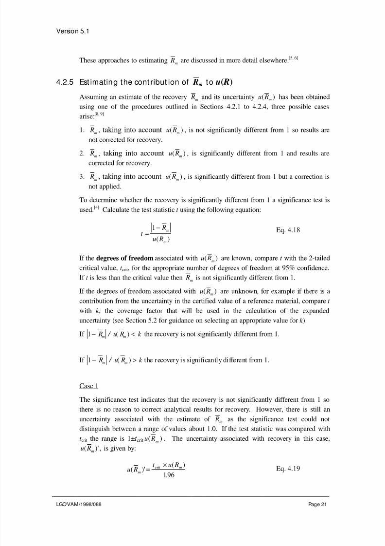
These approaches to estimating Rm
are discussed in more detail elsewhere.[5, 6]
4.2.5 Est imating the cont ribut ion of R m to u( R)
Assuming an estimate of the recovery Rm and its uncertainty u Rm( ) has been obtained
using one of the procedures outlined in Sections 4.2.1 to 4.2.4, three possible cases
arise:[8, 9]
1. Rm
, taking into account u Rm
( ) , is not significantly different from 1 so results are
not corrected for recovery.
2. Rm
, taking into account u Rm
( ) , is significantly different from 1 and results are
corrected for recovery.
3. Rm
, taking into account u Rm
( ) , is significantly different from 1 but a correction is
not applied.
To determine whether the recovery is significantly different from 1 a significance test is
used.[4]
Calculate the test statistic t using the following equation:
t R
u R
m
m
=−1
( )
Eq. 4.18
If the degrees of freedom associated with u Rm
( ) are known, compare t with the 2-tailed
critical value, t crit, for the appropriate number of degrees of freedom at 95% confidence.
If t is less than the critical value then Rm
is not significantly different from 1.
If the degrees of freedom associated with u Rm
( ) are unknown, for example if there is a
contribution from the uncertainty in the certified value of a reference material, compare t
with k , the coverage factor that will be used in the calculation of the expanded
uncertainty (see Section 5.2 for guidance on selecting an appropriate value for k ).
If 1− < R u R k m m / ( ) the recovery is not significantly different from 1.
If 1 − > R u R k m m / ( ) the recovery is significantly different from 1.
Case 1
The significance test indicates that the recovery is not significantly different from 1 so
there is no reason to correct analytical results for recovery. However, there is still an
uncertainty associated with the estimate of Rm
as the significance test could not
distinguish between a range of values about 1.0. If the test statistic was compared with
t crit the range is 1±t crit u Rm( ) . The uncertainty associated with recovery in this case,
u Rm
( )' , is given by:
u Rt u R
m
m( )'( )
.
crit=×
196
Eq. 4.19

8/3/2019 At01 VAM Uncertainty
http://slidepdf.com/reader/full/at01-vam-uncertainty 25/90
Version 5.1
LGC/VAM/1998/088 Page 22
If the test statistic was compared with the coverage factor k , the range is1 ± ×k u Rm
( ) .
In this case the uncertainty associated with Rm
is taken as u Rm
( ) .
To convert to a relative standard deviation divide u Rm
( ) or u Rm
( )' by the assumed value
of Rm . In this case Rm = 1 so the standard deviation is equivalent to the relativestandard deviation.
Case 2
As a correction factor is being applied, Rm
is explicitly included in the calculation of the
result. u Rm
( ) is therefore included in the overall uncertainty calculation as the term
u Rm
( ) / Rm
since the correction is multiplicative (see Section 5).
Case 3
In this case the recovery is statistically significantly different from 1, but in the normal
application of the method no correction is applied (i.e., Rm is assumed to equal 1). Theuncertainty must be increased to take account of the fact that the recovery has not been
corrected for. The increased uncertainty, u Rm
( )' ' , is given by:
u RR
k u R
m
m
m( )' ' ( )=
−
+
12
2 Eq. 4.20
where k is the coverage factor which will be used in the calculation of the expanded
uncertainty.
u Rm( )' ' is expressed as a relative standard deviation by dividing by the assumed value of R
m as in case 1.
4.2.6 Estimating R s and u( R s) f rom spiking studies
Where the method scope covers a range of sample matrices and/or analyte concentrations
an additional uncertainty term is required to take account of differences in the recovery of
a particular sample type, compared to the material used to estimate Rm
. This is can be
evaluated by analysing a representative range of spiked samples, covering typical
matrices and analyte concentrations, in replicate. The number of matrices and levels
examined, and the number of replicates for each sample will depend on the method scope.The same guidelines apply as for the precision studies discussed in Section 4.1.
Calculate the mean recovery for each sample (see Eq. 4.12). Rs is assumed to be equal to
1.0, however there will be an uncertainty in this assumption. This appears in the spread
of mean recoveries observed for the different spiked samples. The uncertainty, u( Rs), is
therefore the standard deviation of the mean recoveries for each sample type.
8/3/2019 At01 VAM Uncertainty
http://slidepdf.com/reader/full/at01-vam-uncertainty 26/90
Version 5.1
LGC/VAM/1998/088 Page 23
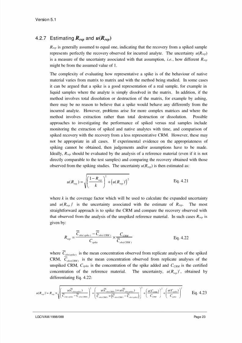
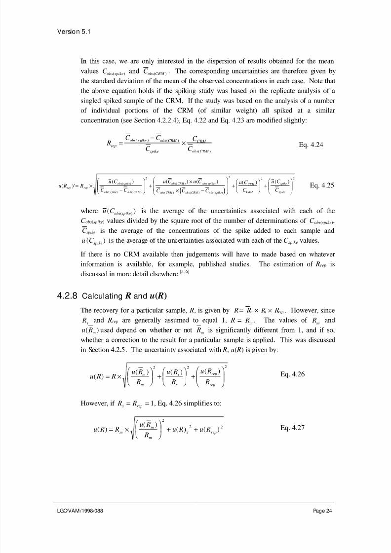
4.2.7 Estimating R rep and u( R rep)
Rrep is generally assumed to equal one, indicating that the recovery from a spiked sample
represents perfectly the recovery observed for incurred analyte. The uncertainty u( Rrep)
is a measure of the uncertainty associated with that assumption, i.e., how different Rrep
might be from the assumed value of 1.
The complexity of evaluating how representative a spike is of the behaviour of native
material varies from matrix to matrix and with the method being studied. In some cases
it can be argued that a spike is a good representation of a real sample, for example in
liquid samples where the analyte is simply dissolved in the matrix. In addition, if the
method involves total dissolution or destruction of the matrix, for example by ashing,
there may be no reason to believe that a spike would behave any differently from the
incurred analyte. However, problems arise for more complex matrices and where the
method involves extraction rather than total destruction or dissolution. Possible
approaches to investigating the performance of spiked versus real samples include
monitoring the extraction of spiked and native analytes with time, and comparison of
spiked recovery with the recovery from a less representative CRM. However, these may
not be appropriate in all cases. If experimental evidence on the appropriateness of
spiking cannot be obtained, then judgements and/or assumptions have to be made.
Ideally, Rrep should be evaluated by the analysis of a reference material (even if it is not
directly comparable to the test samples) and comparing the recovery obtained with those
observed from the spiking studies. The uncertainty u( Rrep) is then estimated as:
( )u R Rk
u Rreprep
rep( ) ( )'= − +1
2
2 Eq. 4.21
where k is the coverage factor which will be used to calculate the expanded uncertainty
and u Rrep( ') is the uncertainty associated with the estimate of Rrep. The most
straightforward approach is to spike the CRM and compare the recovery observed with
that observed from the analysis of the unspiked reference material. In such cases Rrep is
given by:
RC C
C
C
C rep
obs spike obs CRM
spike
CRM
obs CRM
=−
×( ) ( )
( )
Eq. 4.22
where C obs spike( ) is the mean concentration observed from replicate analyses of the spiked
CRM, C obs CRM ( ) is the mean concentration observed from replicate analyses of the
unspiked CRM, C spike is the concentration of the spike added and C CRM is the certified
concentration of the reference material. The uncertainty, u Rrep( )' , obtained by
differentiating Eq. 4.22:
( )u R R
u C
C C
u C u C
C C C
u C
C
u C
C rep rep
obs spike
obs s pi ke obs CRM
obs CRM obs spike
obs CRM obs CRM obs spike
CRM
CRM
spike
spike
( )'( ) ( ) ( ) ( ) ( )
( )
( ) ( )
( ) ( )
( ) ( ) ( )
= ×−
+
×
× −
+
+
2 22 2
Eq. 4.23
8/3/2019 At01 VAM Uncertainty
http://slidepdf.com/reader/full/at01-vam-uncertainty 27/90

8/3/2019 At01 VAM Uncertainty
http://slidepdf.com/reader/full/at01-vam-uncertainty 28/90
Version 5.1
LGC/VAM/1998/088 Page 25
4.3 Evaluation of other sources of uncertaint y
Sources of uncertainty not adequately covered by the precision and trueness experiments
require separate evaluation. For example, a method may require that the sample is
heated to a particular temperature. The method may specify a permitted range about thistemperature, e.g., heat to 100±5 °C. During the precision study the temperature may not
have been varied sufficiently to cover the full range of temperatures permitted in the
method specification. Alternatively there may be no method specification for a particular
parameter. In both cases the effect of changes in the parameter on the result of the
analysis needs to be evaluated. Other sources of uncertainty which may require
evaluation include:
• purity of standards, e.g., if a single batch of material has been used to prepare all
the standards used during the precision study;
• calibration of glassware, e.g., if a single pipette was used throughout theprecision study;
• calibration e.g., if the same set of calibration standards was used throughout the
precision studies.
There are three main sources of data: calibration certificates and manufacturers’
specifications; data published in the literature; specially designed experimental studies.
Each of these is discussed below.
4.3.1 Calibrat ion cert if icates and manufacturers’ specif ications
For many sources of uncertainty, calibration certificates or suppliers’ catalogues provide
the required information:
• Tolerances for volumetric glassware can be obtained from catalogues or the
literature supplied with the item.
• Data on the purity of standards and other reagents can be obtained from the
supplier.
• Calibration uncertainties for balances can be obtained from the calibration
certificate.
Note that the information presented on calibration certificates, etc. may not be in the
form of a standard uncertainty and must therefore be converted before combining with
other uncertainty estimates. Details of how to do this are given in Annex 2.
4.3.2 Publ ished data
As the aim of this guide is to give guidance on obtaining uncertainty estimates during the
method validation stage, it might be expected that very little published data would be
available for a new procedure. This obviously depends on the method, but it may be that

8/3/2019 At01 VAM Uncertainty
http://slidepdf.com/reader/full/at01-vam-uncertainty 29/90
Version 5.1
LGC/VAM/1998/088 Page 26
particular stages of the method have been investigated in the context of other methods so
some data may be available. For example, a sample pre-treatment step such a grinding
or extraction may be common to a number of different methods; or the stability of
samples or reagents used in a procedure may already have been investigated.
4.3.3 Experimental stud ies
If no existing data are available then the uncertainty must be investigated experimentally.
As part of method development and validation, key method parameters are studied to
determine the effect of variations in them on the outcome of the analysis. If a significant
effect is observed for a particular parameter, appropriate control limits are set such that
variations within the limits will not have a significant effect on the outcome of the
analysis. Alternatively, the method is improved by concentrating on the stages of the
method identified as critical. A common method of identifying the critical method
parameters is the ruggedness test. This involves making deliberate variations in themethod and investigating the effect on the result. An established technique for
ruggedness testing is described by the AOAC.[10]
Such a test is also useful for
uncertainty estimation. The results from ruggedness studies can be used in the evaluation
of uncertainties associated with method parameters not adequately covered by the
precision and trueness studies. Such studies can also be used to identify significant
sources of uncertainty which require further study. Suggested procedures for estimating
uncertainty via ruggedness testing are given in the following sections.
4.3.3.1 Designing a ruggedness test
The ruggedness testing procedure described by the AOAC[10]
uses Plackett-Burman
experimental designs.[11]
Such designs allow the investigation of a number of method
parameters in a limited number of experiments. This section focuses on the experimental
design used for investigating seven experimental parameters.
Each of the seven parameters are investigated at two levels. Let A, B, C , D, E , F , G
represent one set of values for the parameters under investigation. Let a, b, c, d , e, f , g
represent the alternative values for the parameters. If control limits have been set in the
method for a parameter (e.g., heat at 100±5 °C) the parameter should be investigated at
the extremes of the permitted range (i.e., 95 °C and 105 °C in the example given). If no
control limits have been specified it is up to the analyst to choose suitable values for the
ruggedness test. This can be based on knowledge gained from similar methods or during
the development of the method being studied, or from knowledge of the normal variation
of the parameter. For example, the method may require that the sample is left to stand at
ambient temperature. The analyst knows that the maximum variation in the laboratory
temperature is 20±5 °C. In the ruggedness test the sample would be left to stand at 15
°C or 25 °C as required by the experimental design.
Variables such as temperature and time are known as continuous variables. Ruggedness
tests can also be used to evaluate the effects of changes in non-continuous variables such
as the type of HPLC column used (e.g., C8 vs.C18).

8/3/2019 At01 VAM Uncertainty
http://slidepdf.com/reader/full/at01-vam-uncertainty 30/90
Version 5.1
LGC/VAM/1998/088 Page 27
The ruggedness test should be carried out on a representative sample. If it is suspected
that particular types of sample may behave in different ways, for example from data
collected in the recovery and precision studies or during the development of the method,
they should be investigated separately and, if possible, the reasons for the differing
response identified.
To investigate seven parameters, a minimum of 8 experiments are required using the
following experimental design:
Determinat ion number
Parametervalue
1 2 3 4 5 6 7 8
A or a A A A A a a a a
B or b B B b b B B b b
C or c C c C c C c C c
D or d D D d d d d D D
E or e E e E e e E e E
F or f F f f F F f f F
G or g G g g G g G G g
Observedresult
s t u v w x y z
The effect of a particular parameter is estimated by subtracting the mean of the resultsobtained with the parameter at the alternative value from the mean of the results obtained
with it at the initial value. For example, for parameter A the difference, D x A, is
calculated from:
D x A =( ) ( )s t u v w x y z+ + +
−+ + +
4 4Eq. 4.28
Calculate the differences for all seven parameters and list them in order of magnitude.
Note that the signs of the differences are unimportant. If variations in one or two
parameters are affecting the analysis then their differences will be substantially larger
than those for the other parameters. To determine whether variations in a parameter have
a significant effect on the result, a significance test is used to determine if the difference
calculated above is significantly different from zero. The procedure is as follows:
1. Obtain an estimate of the within batch method precision, as a standard deviation, from
replicate analysis of a representative sample over a short period of time.
2. Calculate the test statistic t :[12]
t n Dx
s
i=×
×2
Eq. 4.29

8/3/2019 At01 VAM Uncertainty
http://slidepdf.com/reader/full/at01-vam-uncertainty 31/90
Version 5.1
LGC/VAM/1998/088 Page 28
where s is the estimate of the method precision calculated in (1) above, n is the number of
experiments carried out at each level for each parameter (n = 4 for the design given
above), and D xi is the difference calculated for parameter xi.
Compare t with the 2-tailed critical value, t crit, for N -1 degrees of freedom at 95%confidence, where N is the number of determinations used in the estimation of s.
Case 1: If t is less than t crit the difference is not significantly different from zero.
Therefore, variations in the parameter do not have a significant effect on the method
performance.
Case 2: If t is greater than t crit the difference is significantly different from zero.
Therefore, variations in the parameter have a significant effect on the method
performance.
In both cases there is an uncertainty associated with the parameter. Procedures for
estimating the uncertainties are given in the following sections.
4.3.3.2 Calculating uncertainties for case 1 parameters
Although the ruggedness study indicated that variations in the parameter do not
significantly affect the method (i.e., the change in results on varying the parameter is not
significantly different from zero), the significance test could not have distinguished
between values in the range 0±(√2 × t crit × s)/ √n). The uncertainty associated with the
final result y due to parameter xi, is given by:
u y xt s
ni( ( )) crit real
test
=× ×
××
2
196.
δδ
Eq. 4.30
where δreal is the change in the parameter which would be expected when the method is
operating under control in routine use and δtest is the change in parameter that was
specified in the ruggedness test. This term is required to take account of the fact that the
change in a parameter used in the ruggedness test may be much greater than that
observed during normal operation of the method.
If the effect is proportional to the analyte concentration then the uncertainty should be
converted to a relative standard deviation by dividing by an estimate of the mean obtained
from replicate analysis of the sample used in the study under normal conditions, or if this
is not available, by the average of the eight results obtained in the ruggedness test. If,
however, the effect is independent of analyte concentration the uncertainty should be
expressed as a standard deviation (see Section 5).

8/3/2019 At01 VAM Uncertainty
http://slidepdf.com/reader/full/at01-vam-uncertainty 32/90
Version 5.1
LGC/VAM/1998/088 Page 29
4.3.3.3 Calculating uncertainties for case 2 parameters
To calculate the uncertainty for a particular parameter, xi, an estimate of the sensitivity
coefficient, ci, and the uncertainty in the parameter, u( xi), is required.
4.3.3.3.1 Estimating u( xi): For example, a method states that the sample must bedistilled for 120 minutes. The analyst estimates that the variation in the
distillation time in routine application of the method will be ±5 minutes. The
uncertainty in the distillation time is therefore 2.9 minutes (see Annex 2 for
information on calculating standard uncertainties). Alternatively, control
limits can be set for the parameter to ensure that the resulting contribution to
the overall uncertainty is acceptable. If a parameter is already controlled by
specification (such as specifying a temperature as 4 ± 1°C), the specification
limit represents the relevant uncertainty in the parameter, and should be
converted to a standard deviation.
4.3.3.3.2 Estimating ci: If the ruggedness test indicates that the parameter has a
significant effect on the result, the sensitivity coefficient can be estimated
from the results of the study:
cObserved change in result
Change in parameter i
=
Eq. 4.31
If the parameter is found to be a significant source of uncertainty, or if a
better estimate of the effect of the parameter on the result is required, further
experimental study is needed. Evaluate the rate of change of the result with
changes in the parameter by carrying out a number of experiments with the
parameter at a range of different values. Plot a graph of the result versus the
value of the parameter. If the relationship is approximately linear, the
sensitivity coefficient is equivalent to the gradient of the best fit line.
4.3.3.3.3 Calculate the uncertainty in the final result due to parameter xi, u( y( xi)),
using:
u( y( xi)) = u( xi) × ci Eq. 4.32
If the effect is proportional to analyte concentration, convert the uncertainty toa relative standard deviation by dividing u( y( xi)) by y, where y is the result
obtained with the parameter at the value specified in the method.
8/3/2019 At01 VAM Uncertainty
http://slidepdf.com/reader/full/at01-vam-uncertainty 33/90
Version 5.1
LGC/VAM/1998/088 Page 30
5. Calculat ion of combined standard andexpanded uncertaint ies
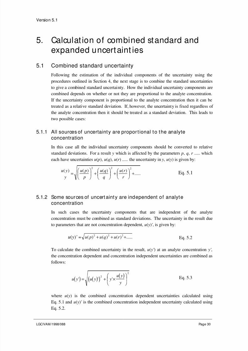
5.1 Combined standard uncertainty
Following the estimation of the individual components of the uncertainty using the
procedures outlined in Section 4, the next stage is to combine the standard uncertainties
to give a combined standard uncertainty. How the individual uncertainty components are
combined depends on whether or not they are proportional to the analyte concentration.
If the uncertainty component is proportional to the analyte concentration then it can be
treated as a relative standard deviation. If, however, the uncertainty is fixed regardless of
the analyte concentration then it should be treated as a standard deviation. This leads to
two possible cases:
5.1.1 All sources of uncertainty are propor t ional to the analyte
concentration
In this case all the individual uncertainty components should be converted to relative
standard deviations. For a result y which is affected by the parameters p, q, r ..... which
each have uncertainties u( p), u(q), u(r ) ..... the uncertainty in y, u( y) is given by:
u y
y
u p
p
u q
q
u r
r
( ) ( ) ( ) ( ).....=
+
+
+
2 2 2
Eq. 5.1
5.1.2 Some sources of uncert ainty are independent of analyteconcentration
In such cases the uncertainty components that are independent of the analyte
concentration must be combined as standard deviations. The uncertainty in the result due
to parameters that are not concentration dependent, u( y)' , is given by:
u( y)' = u p u q u r ( ) ( ) ( ) .....2 2 2+ + + Eq. 5.2
To calculate the combined uncertainty in the result, u( y' ) at an analyte concentration y' ,
the concentration dependent and concentration independent uncertainties are combined as
follows:
( ) ( )( )( )
u y u y yu y
y' ' ' = + ×
2
2
Eq. 5.3
where u( y) is the combined concentration dependent uncertainties calculated using
Eq. 5.1 and u( y)' is the combined concentration independent uncertainty calculated using
Eq. 5.2.
8/3/2019 At01 VAM Uncertainty
http://slidepdf.com/reader/full/at01-vam-uncertainty 34/90
Version 5.1
LGC/VAM/1998/088 Page 31
Note that when the uncertainty estimate is required for a single analyte concentration, the
uncertainty components can be combined as either standard deviations or relative
standard deviations; it will make no difference to the final answer.
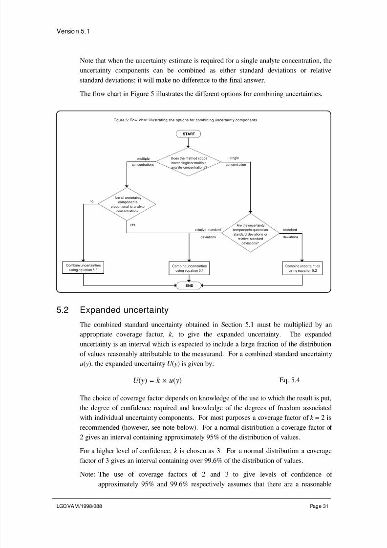
The flow chart in Figure 5 illustrates the different options for combining uncertainties.
no
multiple
concentrations
single
concentration
Does the method scope
cover single or multiple
analyte concentrations?
Are all uncertainty
components
proportional to analyte
concentration?
Are the uncertainty
components quoted as
standard deviations or
relative standard
deviations?
Combine uncertainties
using equation 5.1
Combine uncertainties
using equation 5.2
Combine uncertainties
using equation 5.3
relative standard
yes
standard
Figure 5: Flow chart il lustrating t he options for combining uncertainty components
deviations deviations
START
END
5.2 Expanded uncertainty
The combined standard uncertainty obtained in Section 5.1 must be multiplied by an
appropriate coverage factor, k , to give the expanded uncertainty. The expanded
uncertainty is an interval which is expected to include a large fraction of the distribution
of values reasonably attributable to the measurand. For a combined standard uncertainty
u( y), the expanded uncertainty U ( y) is given by:
U ( y) = k × u( y) Eq. 5.4
The choice of coverage factor depends on knowledge of the use to which the result is put,
the degree of confidence required and knowledge of the degrees of freedom associated
with individual uncertainty components. For most purposes a coverage factor of k = 2 is
recommended (however, see note below). For a normal distribution a coverage factor of
2 gives an interval containing approximately 95% of the distribution of values.
For a higher level of confidence, k is chosen as 3. For a normal distribution a coverage
factor of 3 gives an interval containing over 99.6% of the distribution of values.
Note: The use of coverage factors of 2 and 3 to give levels of confidence of
approximately 95% and 99.6% respectively assumes that there are a reasonable
8/3/2019 At01 VAM Uncertainty
http://slidepdf.com/reader/full/at01-vam-uncertainty 35/90
Version 5.1
LGC/VAM/1998/088 Page 32
number of degrees of freedom associated with the estimates of the major
contributions to the uncertainty budget. In this guide it is recommended that at
least 10 determinations are carried out in the precision and trueness studies. If it is
not possible to obtain this many replicates and either of these factors dominate the
uncertainty budget, the coverage factor should be obtained from the table of
critical values for the Student t test. For example, if the dominant contribution to
the uncertainty budget was based on only 4 determinations this would give 3
degrees of freedom. The 2-tailed t crit value at the 95% confidence level is 3.182. It
can therefore be seen that using uncertainty estimates based on only a small
number of determinations will have a significant effect on the coverage factor and
hence on the expanded uncertainty.

8/3/2019 At01 VAM Uncertainty
http://slidepdf.com/reader/full/at01-vam-uncertainty 36/90
Version 5.1
LGC/VAM/1998/088 Page 33
6. Report ing uncertaint y
6.1 Report ing expanded uncertainty
The Eurachem Guide[2]
gives the following guidance:
Unless otherwise required, the result y should be stated together with the expanded
uncertainty, U ( y), calculated using a coverage factor of k = 2 (or other appropriate
coverage factor, see Section 5.2). The following form is recommended:
“(result): y ± U ( y) (units)
[where] the reported uncertainty is [an expanded uncertainty as defined in the
International Vocabulary of Basic and General terms in Metrology, 2nd, ed., ISO, 1993]calculated using a coverage factor of 2, [which gives a level of confidence of
approximately 95%.]”
Terms in [ ] may be omitted or abbreviated as appropriate.
6.2 Report ing standard uncertainty
The Eurachem Guide[2]
gives the following guidance:
When uncertainty is expressed as the combined standard uncertainty u( y) the following
form is recommended:
“(result): y (units) [with a] standard uncertainty of u( y) (units) [where standard
uncertainty is defined in the International Vocabulary of Basic and General terms in
Metrology, 2nd, ed., ISO, 1993 and corresponds to one standard deviation.]”
The use of the symbol ± is not recommended when using standard uncertainty.
6.3 Documentation
A simple proforma for summarising uncertainty budgets is given in Annex 5. This can
be used to summarise details of the sources of uncertainty included in the budget, how
they were estimated and their magnitudes. There is also a section for the combined
standard and expanded uncertainty.

8/3/2019 At01 VAM Uncertainty
http://slidepdf.com/reader/full/at01-vam-uncertainty 37/90
Version 5.1
LGC/VAM/1998/088 Page 34
Annex 1: Cause and Ef fect Analysis
As discussed in Section 3, uncertainty estimation requires the production of a structured list of
possible sources of uncertainty. One way of producing such a list is cause and effect
analysis.[13]
The principles of the construction of cause and effect diagrams are described fully
elsewhere,[13]
and detailed discussions of their application to uncertainty estimation, with
examples, have been published.[14, 15]
The use of cause and effect diagrams has three main
stages: construction, refinement and experimental design (also called reconciliation). An outline
of the process is presented below.
A1.1 Construction of a cause and eff ect diagram
A cause and effect diagram consists of a hierarchical structure of “causes” which culminate in a
single outcome or “effect”. A typical diagram for an analytical method is given in Figure A1.1.
In terms of uncertainty estimation, the “effect” is the result obtained from the analysis. The
main branches feeding into it represent the parameters used in the calculation of the result.
Combining the uncertainties associated with these parameters will give the uncertainty in the
final result. The stages in the construction are:
A1.1.1 Write the complete equation used to calculate the result, including any intermediate
calculations. The parameters in the equation form the main branches of the diagram. It is
almost always necessary to add a main branch representing overall bias, usually as recovery.
A1.1.2 Consider each branch in turn and add additional branches representing effects which will
contribute to the uncertainties in the parameters identified in A1.1.1. For example, theuncertainty in the weight of sample taken for analysis will have contributions from the balance
precision and calibration. Branches representing these terms should therefore feed into the main
branch representing the sample weight.
A1.1.3 For each branch added in A1.1.2, add further branches representing any additional contributory
factors. Continue the process until the effects become sufficiently remote.
A1.2 Refinement of the cause and effect diagram
Refinement of the diagram involves the resolution of duplicate terms and rearrangement of the
branches to clarify contributions and group related causes. This process results in a simplified
cause and effect diagram which can be used as a checklist to ensure that all sources of
uncertainty have been considered in the uncertainty budget. Duplications of terms in the
diagram are resolved using the rules given in Section 3.4.
Figure A1.2 shows a typical cause and effect diagram after refinement.
A1.3 Experimental design
The final stage in the process is the planning of experiments which will provide the information
required to obtain an estimate of the combined uncertainty for the method. Initially, two sets of
experiments are carried out - a precision study and a trueness study. These experiments are

8/3/2019 At01 VAM Uncertainty
http://slidepdf.com/reader/full/at01-vam-uncertainty 38/90
Version 5.1
LGC/VAM/1998/088 Page 35
planned in such a way that as many of the sources of uncertainty identified in the cause and
effect diagram as possible are covered. The diagram is used as a checklist, and those
parameters not adequately covered by the precision and trueness experiments are evaluated
separately. Section 4 discusses the types of experiments required and gives details of how the
data obtained are used to calculate uncertainty.
Key to Figure A1.1 and Figure A1.2
Equation used to calculate the concentration of all-trans retinol, Call trans− in µg 100 g-1
, in a
sample of infant formula:
CA V C
A Wal l t rans
S F STD
STD S
− =× ×
×
where:
AS is the peak area recorded for the sample solution;
ASTD is the peak area recorded for the standard solution;
VF is the final volume of the sample solution (ml);
WS is the weight of sample taken for analysis (g);
CSTD is the concentration of the standard solution (µg ml-1).
In the cause and effect diagrams:
C flask/pipette calibration;
T temperature effects;
BC balance calibration;
L balance linearity.
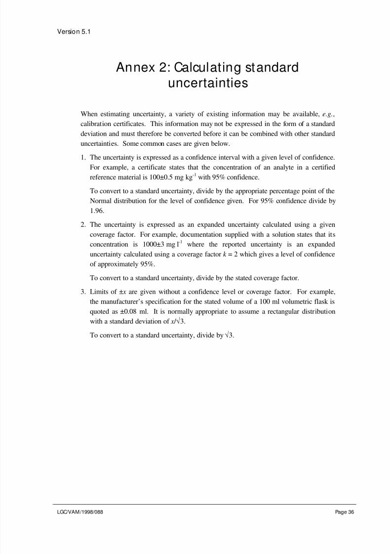
8/3/2019 At01 VAM Uncertainty
http://slidepdf.com/reader/full/at01-vam-uncertainty 39/90
Version 5.1
LGC/VAM/1998/088 Page 36
Annex 2: Calculating standarduncertainties
When estimating uncertainty, a variety of existing information may be available, e.g.,
calibration certificates. This information may not be expressed in the form of a standard
deviation and must therefore be converted before it can be combined with other standard
uncertainties. Some common cases are given below.
1. The uncertainty is expressed as a confidence interval with a given level of confidence.
For example, a certificate states that the concentration of an analyte in a certified
reference material is 100±0.5 mg kg-1
with 95% confidence.
To convert to a standard uncertainty, divide by the appropriate percentage point of theNormal distribution for the level of confidence given. For 95% confidence divide by
1.96.
2. The uncertainty is expressed as an expanded uncertainty calculated using a given
coverage factor. For example, documentation supplied with a solution states that its
concentration is 1000±3 mg l-1
where the reported uncertainty is an expanded
uncertainty calculated using a coverage factor k = 2 which gives a level of confidence
of approximately 95%.
To convert to a standard uncertainty, divide by the stated coverage factor.
3. Limits of ± x are given without a confidence level or coverage factor. For example,the manufacturer’s specification for the stated volume of a 100 ml volumetric flask is
quoted as ±0.08 ml. It is normally appropriate to assume a rectangular distribution
with a standard deviation of x / √3.
To convert to a standard uncertainty, divide by √3.

8/3/2019 At01 VAM Uncertainty
http://slidepdf.com/reader/full/at01-vam-uncertainty 40/90
Version 5.1
LGC/VAM/1998/088 Page 37
Annex 3: Def init ions
Bias
The difference between the expectation of the test results and an accepted reference
value.[16]
Note: Bias is the total systematic error as contrasted to random error. There may be one or
more systematic error components contributing to the bias. A larger systematic
difference from the accepted reference value is reflected by a larger bias value.
Coverage factor
The numerical factor, k , used as a multiplier of the combined standard uncertainty in
order to obtain an expanded uncertainty.
[1]
Note: A coverage factor is typically in the range 2 to 3. A coverage factor of 2 gives a level of
confidence of approximately 95%.
Crit ical value
The critical value (e.g. t crit in a t -test) is the tabulated value of the test statistic obtained in
a significance test. The critical value is obtained from statistical tables by reading the
value given for the appropriate number of degrees of freedom and the desired level of
confidence.[4]
In this guide, two-tailed t crit values at the 95% confidence level are always
used.
Degrees of f reedom
The term n-1 in the expression for the sample standard deviation, s, is called the number
of degrees of freedom (abbreviated to dof or ν in statistical tables). In general it is the
number of data points, n, less the number of parameters already estimated from the data.
In the expression for the sample standard deviation the number of degrees of freedom is
n-1 as the mean has already been estimated from the data. Knowledge of the number of
degrees of freedom is needed for obtaining the appropriate critical value from statistical
tables for significance tests. In general it is equivalent to n-1.
Expanded uncertainty
Quantity defining an interval about the result of a measurement that may be expected to
encompass a large fraction of the distribution of values that could reasonably be
attributed to the measurand.[1]
The expanded uncertainty, U ( y), is calculated from the
combined standard uncertainty u( y) and a coverage factor k using:
U ( y) = k × u( y)
8/3/2019 At01 VAM Uncertainty
http://slidepdf.com/reader/full/at01-vam-uncertainty 41/90
Version 5.1
LGC/VAM/1998/088 Page 38
F-test
The F-test is a significance test used to compare two variances, s1
2and s2
2, where s is
the standard deviation. Calculate the test statistic:
F =s
s
1
2
2
2
where s1
2is the larger of the two variances (this will guarantee that F≥1). Compare F
with the appropriate critical value, Fcrit, at n1-1 and n2-1 degrees of freedom. If F is less
than Fcrit there is no significant difference between the variances. For a 2-tailed test at the
95% confidence level, the appropriate critical value is obtained from statistical tables for
the 97.5% confidence level.[4]
Measurement uncertainty
Parameter associated with the result of a measurement, that characterises the dispersion
of values that could reasonably be attributed to the measurand.[17]
Note: The parameter may be, for example, a standard deviation (or given multiple of it), or the
width of a confidence interval. Uncertainty of measurement comprises, in general, many
components. Some of these components may be evaluated from the distribution of the
results of a series of measurements and can be characterised by experimental standard
deviations. The other components, which can also be characterised by standard
deviations, are evaluated from assumed probability distributions based on experience or
other information. It is understood that the result of the measurement is the best
estimate of the value of the measurand and that all components of uncertainty, including
those arising from systematic effects, contribute to the dispersion.
Precision
The closeness of agreement between independent test results obtained under stipulated
conditions.[16]
Note: Precision depends only on the distribution of random errors and does not relate to the
true value or specified value. The measure of precision is usually expressed in terms of
imprecision and calculated as a standard deviation of the test results.
Recovery
The ratio of the observed value to the expected value.
Note: The expected value can be either the certified value of a reference material or the
concentration of a fortified or spiked sample. In analytical chemistry, recovery is often
used as a measure of the trueness of a method.

8/3/2019 At01 VAM Uncertainty
http://slidepdf.com/reader/full/at01-vam-uncertainty 42/90
Version 5.1
LGC/VAM/1998/088 Page 39
Relative standard deviat ion
The relative standard deviation, RSD, of a set of results with standard deviation s and
mean x is given by:
RSDs
x=
Sample standard deviat ion
The standard deviation of n results with a mean x is given by:
s x x
n
i
i
n
= −−
=∑ ( )2
1
1
Sensit ivi ty coeff icient
The sensitivity coefficient describes how the observed output varies with changes in the
input parameter. For example, for a result y and a parameter xi, the sensitivity
coefficient ci describing the effect of changes in xi on y is given by:
cObserved change in y
Change in xi
i
=
Signif icance test
A statistical test used to decide whether there are significant differences between the
properties of different sets of data at a given level of confidence. A test statistic is
calculated and compared with a tabulated critical value. If the test statistic is greater
than the critical value this indicates a significant difference between the properties being
compared. Examples of significance tests include the t -test which can be used to
compare the mean of a set of results with a stated value, or to compare the means of two
independent sets of results; and the F-test which is used to compare the variances of two
sets of data.[4]

8/3/2019 At01 VAM Uncertainty
http://slidepdf.com/reader/full/at01-vam-uncertainty 43/90
Version 5.1
LGC/VAM/1998/088 Page 40
Standard deviation of the mean
The standard deviation of the mean, s x
, of n samples with standard deviation s is given
by:
ss
n x
=
Standard uncertainty
Uncertainty of the result of a measurement expressed as a standard deviation.[1]
For a
result xi, the standard uncertainty is u( xi).
Trueness
The closeness of agreement between the average value obtained from a large set of test
results and an accepted reference value.[16]
Note: The measure of trueness is normally expressed in terms of bias.
Uncertainty budget
List of parameters and their associated uncertainties which contribute to the uncertainty
for the method as a whole. The individual uncertainties in the uncertainty budget are
combined to give the standard and expanded uncertainties for the method.

8/3/2019 At01 VAM Uncertainty
http://slidepdf.com/reader/full/at01-vam-uncertainty 44/90
Version 5.1
LGC/VAM/1998/088 Page 41
Annex 4: Worked examples
A4.1 The determination of vitamin A and vitamin E in infant formula
A4.1.1 Outline of method
The method was developed for the determination of tocopherol, retinol and carotene
isomers in a range of food stuffs. This example considers the validation and calculation
of an uncertainty estimate specifically for the determination of all-trans retinol (vitamin
A) and α-tocopherol (vitamin E) in infant formula. The homogenised sample is
hydrolysed to release the retinol and tocopherol isomers. These are then extracted into
mixed ethers and the extract concentrated. Portions of the extract are chromatographed
on different HPLC systems to separate and quantify the isomers required. A normalphase system is used for the determination of α-tocopherol whilst a reversed phase
system is used for the determination of all-trans retinol. In each case calibration is by
means of a single standard prepared by serial dilution of a stock solution. The
concentration of the analyte in a sample, C vit, is given by:
C vitS F STD
STD S
A V C
A W=
× ××
where:
AS is the peak area recorded for the sample solution;ASTDis the peak area recorded for the standard solution;
VF is the final volume of the sample solution (ml);
WS is the weight of sample taken for analysis (g);
CSTD is the concentration of the standard solution (µg ml-1
).
A flow diagram illustrating the stages in the method is presented in Figure A4.1 and
cause and effect diagrams are given in Annex 1.
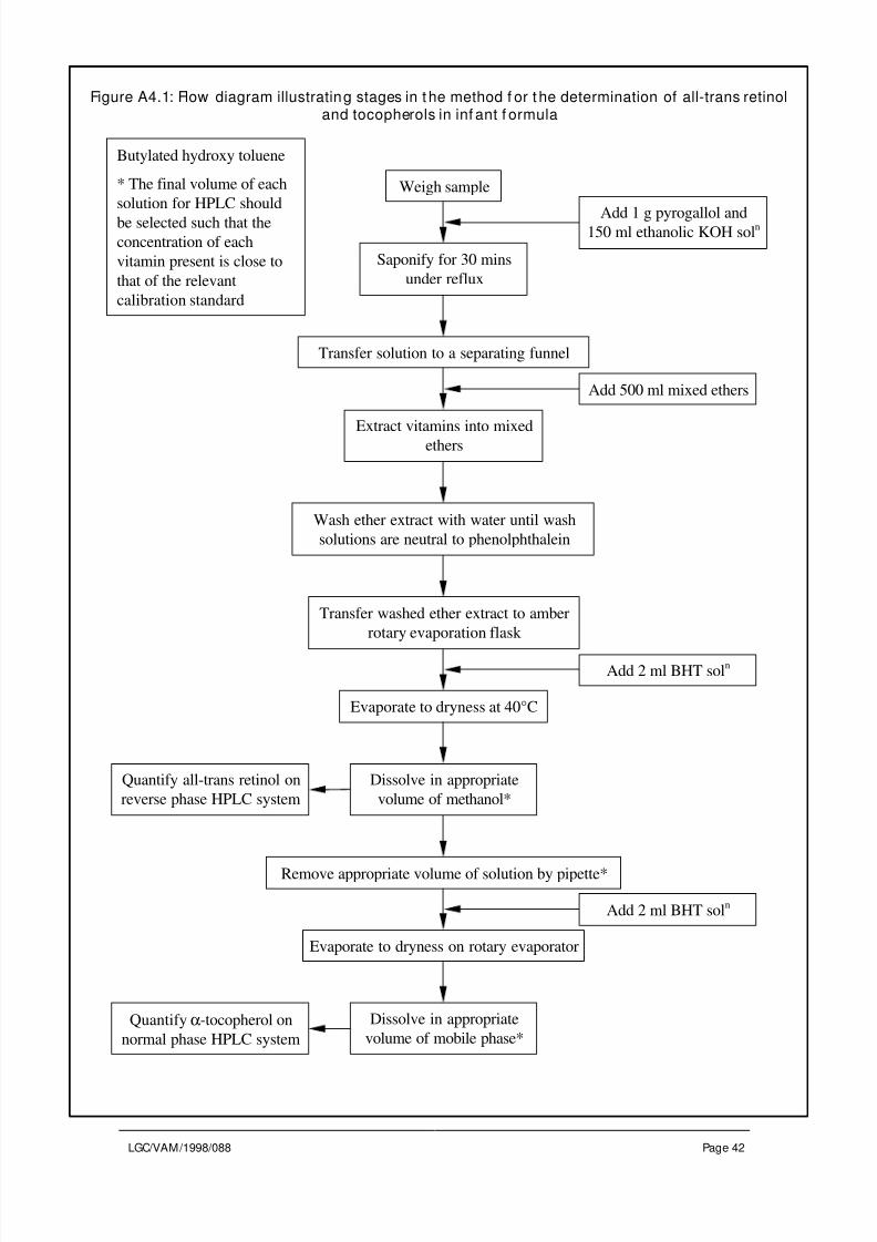
8/3/2019 At01 VAM Uncertainty
http://slidepdf.com/reader/full/at01-vam-uncertainty 45/90
LGC/VAM/1998/088 Page 42
Weigh sample
Saponify for 30 mins
under reflux
Add 1 g pyrogallol and150 ml ethanolic KOH sol
n
Transfer solution to a separating funnel
Add 500 ml mixed ethers
Extract vitamins into mixed
ethers
Wash ether extract with water until wash
solutions are neutral to phenolphthalein
Transfer washed ether extract to amber
rotary evaporation flask
Add 2 ml BHT soln
Evaporate to dryness at 40°C
Dissolve in appropriate
volume of methanol*
Quantify all-trans retinol on
reverse phase HPLC system
Remove appropriate volume of solution by pipette*
Add 2 ml BHT soln
Evaporate to dryness on rotary evaporator
Dissolve in appropriate
volume of mobile phase*
Quantify α-tocopherol on
normal phase HPLC system
Butylated hydroxy toluene
* The final volume of each
solution for HPLC should
be selected such that the
concentration of each
vitamin present is close to
that of the relevant
calibration standard
Figure A4.1: Flow diagram illustrating stages in t he method f or t he determination of all-trans retinoland tocopherols in inf ant f ormula

8/3/2019 At01 VAM Uncertainty
http://slidepdf.com/reader/full/at01-vam-uncertainty 46/90
Version 5.1
LGC/VAM/1998/088 Page 43
A4.1.2 Precision study
A survey of the nutritional labelling of commercially available infant formula indicated
that that they were all of broadly comparable composition (fat, protein and carbohydrate
levels) and contained similar concentrations of vitamin A and vitamin E. Three samples
were chosen to cover the widest possible range of vitamin concentrations. Each sample
was analysed a total of four times, in four separate extraction and HPLC runs. For each
HPLC run fresh calibration standards and mobile phase were prepared. In addition, a
certified reference material (SRM 1846) was analysed in replicate for the estimation of
Rm
(see below). These results were included in the precision study. The results are
summarised in Table A4.1.§
Table A4.1: Summary o f result s from precision studies on the determination o f all-trans retinol andα-tocopherol
all-trans ret inol α-tocopherol
Sample mean(mg kg-1)
standarddeviation(mg kg-1)
relativestandarddeviation
n mean(mg kg-1)
standarddeviation(mg kg-1)
relativestandarddeviation
n
Infant formula A 9.67 0.146 0.0151 4 64.08 2.411 0.0376 4
Infant formula B 10.40 0.247 0.0238 4 69.05 2.156 0.0312 4
Infant formula C 6.67 0.217 0.0325 4 171.93 7.959 0.0463 4
SRM 1846 5.32 0.285 0.0536 6 278.51 10.663 0.0383 6
The standard deviations observed for all-trans retinol were of a similar order of
magnitude. This indicates that within the range of analyte concentrations studied, the
standard deviation is independent of analyte concentration. In this case, the uncertainty
associated with method precision, u(P), for samples with all-trans retinol concentrations
ranging from approximately 5 mg kg-1
to 10 mg kg-1
, was estimated as the pooled
standard deviation. This was obtained using Eq. 4.1:
( ) ( ) ( ) ( )s pool =
× + × + × + ×
+ +
=
3 0146 3 0 247 3 0 217 5 0 285
3 3 3 50238
2 2 2 2. .
+
. ..
u(P) for all-trans retinol is therefore 0.238 mg kg-1
.
§
Note: The examples given in Annex 4 were calculated using a spreadsheet. The values presented in
the tables and equations have been rounded. Reproducing the calculations with the values given maytherefore result in slightly differing answers.

8/3/2019 At01 VAM Uncertainty
http://slidepdf.com/reader/full/at01-vam-uncertainty 47/90
Version 5.1
LGC/VAM/1998/088 Page 44
For α-tocopherol, the relative standard deviations observed for the different samples were
all of a similar order of magnitude. This indicates that the standard deviation is
approximately proportional to analyte concentration, across the range studied. In such
cases it is appropriate to pool the relative standard deviations to obtain the estimate of
u(P), using Eq. 4.2:
( ) ( ) ( ) ( ) RSD
pool=
× + × + × + ×
+ + +
=
3 00376 3 0 0312 3 0 0463 5 0 0383
3 3 3 500387
2 2 2 2. . .
..
u(P)/ P for α-tocopherol is therefore 0.0387 as a relative standard deviation.
A4.1.3 Trueness study
Calculation of R m and u( R m )
In this case a certified reference material, SRM 1846 produced by the National Institute
of Standards and Technology (NIST), was available. The CRM is an infant formula
certified for a number of vitamins, including all-trans retinol and α-tocopherol. Six
portions of the CRM were analysed. The results, together with the certified values for
the material, are summarised in Table A4.2.
Table A4.2: Result s from the analysis of inf ant formula SRM 1846
Cert if ied values Observed values
Analyte Concentrat ion
C CRM
(mg kg-1)
Quoteduncertainty
(mg kg-1)1
Standarduncertainty
u(C CRM )(mg kg-1)2
Mean
C obs
(mg kg-1)
standarddeviation
s obs
(mg kg-1)
all-trans retinol 5.84 0.68 0.35 5.32 0.285
α-tocopherol 271 25 12.8 278.51 10.663
1The quoted uncertainty is an expanded uncertainty given at the 95% confidence level.
2
The standard uncertainty is obtained by dividing the expanded uncertainty by 1.96.
Eq. 4.3 and Eq. 4.4 were used to calculate Rm
and u Rm
( ) respectively.
For all-trans retinol:
Rm
= =5 32 584 0 911. / . .

8/3/2019 At01 VAM Uncertainty
http://slidepdf.com/reader/full/at01-vam-uncertainty 48/90
Version 5.1
LGC/VAM/1998/088 Page 45
u Rm( ) = ××
+
=0911
0 285
6 5 32
0 35
5840 0581
2
2
2
..
.
.
..
Similar calculations for α-tocopherol gave values of Rm = 1.028 and u Rm( ) = 0.0511.
To determine the contribution of Rm
to the combined uncertainty, the value calculated
above was compared with 1, using Eq. 4.18. For all-trans retinol:
t =−
=1 0 911
00581153
.
..
In this case, t was compared with the coverage factor, k = 2. As t is less than two there
is no evidence to suggest that Rm
is significantly different from 1. Rm
was therefore
assumed to equal 1 with an uncertainty, u Rm( ) , of 0.0581 (see Section 4.2.5, case 1). Asimilar calculation for α-tocopherol also indicated that R
mwas not significantly different
from 1. u Rm
( ) was therefore estimated as 0.0511.
Calculation of u( R s)
Rs was estimated from spiking studies on infant formula A used in the precision study. It
was not possible to produce a homogeneous bulk spiked sample so individual portions of
the infant formula were spiked at the required concentration. Samples were prepared at
the concentrations indicated in Table A4.3. Four samples were analysed at each
concentration, in separate extraction and HPLC batches. The samples were spiked byadding solutions of all-trans retinol and α-tocopherol to approximately 10 g of sample in
a saponification flask, prior to the addition of any other reagents. The mean recovery for
each sample was calculated using Eq. 4.12. C native was taken as the mean of the results
obtained from the precision study. The results are summarised in Table A4.3.
Table A4.3: Summary of results from the study of R s for t he determination of all-trans retino l
and α-tocopherol
all-trans retinol α-tocopherol
Spiking level Approxtarget
concentration(mg kg-1)
Meanrecovery
n Approxtarget
concentration(mg kg-1)
Meanrecovery
n
1 14.0 0.981 4 84.0 1.028 4
2 18.0 0.991 4 99.0 1.103 4
3 22.0 0.996 4 114.0 1.167 4
u( R s ) 0.00767 u( R s ) 0.0696
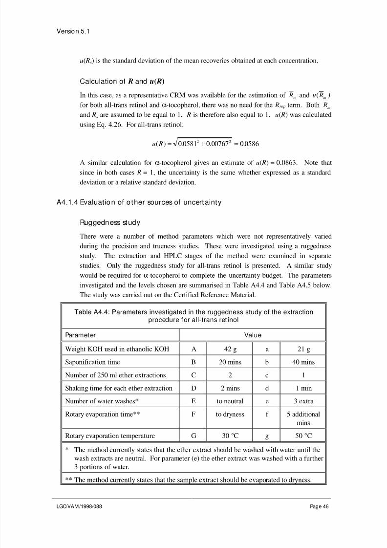
8/3/2019 At01 VAM Uncertainty
http://slidepdf.com/reader/full/at01-vam-uncertainty 49/90
Version 5.1
LGC/VAM/1998/088 Page 46
u( Rs) is the standard deviation of the mean recoveries obtained at each concentration.
Calculation of R and u( R)
In this case, as a representative CRM was available for the estimation of Rm and u Rm( )for both all-trans retinol and α-tocopherol, there was no need for the Rrep term. Both R
m
and Rs are assumed to be equal to 1. R is therefore also equal to 1. u( R) was calculated
using Eq. 4.26. For all-trans retinol:
u R( ) = + =0 0581 0 00767 0 05862 2. . .
A similar calculation for α-tocopherol gives an estimate of u( R) = 0.0863. Note that
since in both cases R = 1, the uncertainty is the same whether expressed as a standard
deviation or a relative standard deviation.
A4.1.4 Evaluation of o ther sources of uncertainty
Ruggedness study
There were a number of method parameters which were not representatively varied
during the precision and trueness studies. These were investigated using a ruggedness
study. The extraction and HPLC stages of the method were examined in separate
studies. Only the ruggedness study for all-trans retinol is presented. A similar study
would be required for α-tocopherol to complete the uncertainty budget. The parameters
investigated and the levels chosen are summarised in Table A4.4 and Table A4.5 below.The study was carried out on the Certified Reference Material.
Table A4.4: Parameters investigated in the ruggedness study of the extractionprocedure for all-trans ret inol
Parameter Value
Weight KOH used in ethanolic KOH A 42 g a 21 g
Saponification time B 20 mins b 40 mins
Number of 250 ml ether extractions C 2 c 1
Shaking time for each ether extraction D 2 mins d 1 min
Number of water washes* E to neutral e 3 extra
Rotary evaporation time** F to dryness f 5 additional
mins
Rotary evaporation temperature G 30 °C g 50 °C
* The method currently states that the ether extract should be washed with water until the
wash extracts are neutral. For parameter (e) the ether extract was washed with a further
3 portions of water.
** The method currently states that the sample extract should be evaporated to dryness.

8/3/2019 At01 VAM Uncertainty
http://slidepdf.com/reader/full/at01-vam-uncertainty 50/90
Version 5.1
LGC/VAM/1998/088 Page 47
For parameter (f) the evaporation was continued for a further 5 minutes after dryness
had been reached.
Table A4.5: Parameters investigated in the ruggedness study of the HPLC procedurefor the determination of all-trans retinol
Parameter Value
Column age A' new a' old
Flow rate B' 0.8 ml min-1
b' 1.2 ml min-1
Dummy variable C' + c' -
Mobile phase composition
(methanol/water)
D' 90/10 d' 95/5
Injection volume E' 15 µl e' 25 µl
Detection wavelength F' 320 nm f' 330 nm
Column temperature G' 30 °C g' oven off
Results
The results from the ruggedness studies were evaluated as described in Section 4.3.3.
Ext ract ion and clean-up stage
The results obtained from the ruggedness testing of the extraction procedure for all-trans
retinol are presented in Table A4.6. The differences for each parameter, D x A to D xG,
were calculated as described in Section 4.3.3.1.
Table A4.6: Results form the ruggedness testing of the extraction of all-transretinol from infant formula
Observed result (mg kg -1)
s t u v w x y z
5.25 3.98 4.22 4.43 5.51 4.78 4.35 4.96
Calculated di f ferences
D x A D x B D xC D x D D x E D x F D xG
-0.4329 0.3898 0.2948 -0.1009 0.2387 0.7036 0.03608
The precision for the method had previously been estimated as 0.238 mg kg-1
with 14
degrees of freedom (see Section A4.1.2). Using Eq. 4.29, t values were calculated for

8/3/2019 At01 VAM Uncertainty
http://slidepdf.com/reader/full/at01-vam-uncertainty 51/90
Version 5.1
LGC/VAM/1998/088 Page 48
each parameter. These were then compared with the critical value t crit = 2.145 (2-tailed,
ν = 14, 95% confidence). The results are presented below:
Table A4.7: Identif ication of parameters having a signif icant effect onthe extraction of all-trans retinol f rom infant formula
Parameter t value Significanteffect at 95%confidence?
Weight KOH used in ethanolic KOH 2.573 Yes
Saponification time 2.316 Yes
Number of 250 ml ether extractions 1.752 No
Shaking time for each ether extraction 0.599 No
Number of water washes 1.419 No
Rotary evaporation time 4.181 Yes
Rotary evaporation temperature 0.214 No
In cases where the effect of a parameter was found not to be significant, Eq. 4.30 was
used to calculate the uncertainty:
u y xireal
test
real
test
( ( )) = × ×× × = ×2 2 145 0 2384 196
0184. ..
.δδ δδ
Number of ether ext ract ions
The method specifies two ether extractions. In the ruggedness study, the effect of using
only one ether extraction was investigated. The results indicated that using only one
extraction reduced the recovery of all-trans retinol, although the effect was not
significant. If the method is applied correctly it is unlikely that δreal would equal δtest.
However, there is likely to be some variation in the efficiency of the extractions from
analysis to analysis, due to variations in the vigour with which the mixture is shaken.
This effect will be covered by the estimate of uncertainty associated with precision. For
these reasons, an additional uncertainty has not been included for this parameter.
Shaking t ime for ether ext ract ions
The method was developed using a shaking time of 2 minutes per extraction. In the
ruggedness test this was reduced to 1 minute. δtest is therefore equal to 1 minute. It is
estimated that during normal operation of the method, the shaking time might vary
between 1.5 minutes and 2.5 minutes. δreal is therefore also 1 minute. u( y( x D)) is
therefore 0.184 mg kg-1
.

8/3/2019 At01 VAM Uncertainty
http://slidepdf.com/reader/full/at01-vam-uncertainty 52/90
Version 5.1
LGC/VAM/1998/088 Page 49
Number of w ater w ashes
The method currently specifies that the ether extract should be washed with 150 ml
portions of water until the wash solution is neutral to phenolphthalein. The results of the
ruggedness test indicate that additional washes of the extract beyond this leads to lower
results. In the ruggedness study the effect of three extra washes was investigated
(δtest = 3). During routine use of the method it was considered unlikely that as many as
three extra washes would be carried out. However, one additional wash may be likely,
particularly if neutrality has only just been reached on the previous wash. δreal was
therefore estimated as being equal to 1. The uncertainty, u( y( x E )), is therefore 0.0613.
Rotary evaporation t emperature
The method has been developed using a rotary evaporation temperature of 40°C. It is
estimated that this is controlled to ±2°C in normal use ( i.e., δreal = 4°C). In the
ruggedness test the temperature was set at 30°C and 50°C, giving a δtest value of 20°C.u( y( xG)) is therefore 0.0368 mg kg
-1.
For parameters identified as having a significant effect on the extraction, the procedure
described in Section 4.3.3.3 was followed.
Weight of potassium hydroxide used to prepare ethanolic potassium hydroxide solution
Under normal operating conditions, 42±0.1 g potassium hydroxide is used in the
preparation of the ethanolic potassium hydroxide solution required for the saponification
reaction. In the ruggedness study the amount of potassium hydroxide used was reduced
by 21 g. This resulted in a difference, D x A, of -0.4329 mg kg-1. Using Eq. 4.31, thesensitivity coefficient, c A, was calculated as:
c A = =0 4329
210 0206
.. mg kg
-1g
-1
The uncertainty in the parameter, u( x A), was obtained from the control limit on the weight
of potassium hydroxide specified in the method, assuming a rectangular distribution.
Therefore, u( x A) = 0.1/ √3 = 0.0577 g. The uncertainty in the final result due to
variations in parameter A, u( y( x A)) was calculated using Eq. 4.32:
u y x A
( ( )) = × =0 0577 0 0206 0 00119. . . mg kg-1
Saponif ication t ime
The method was developed using a saponification time of 30 minutes. It is estimated that
during routine use of the method this will vary by ±5 minutes, giving an uncertainty, u B,
of 2.89 minutes (assuming a rectangular distribution). In the ruggedness study the
parameter was varied from 20 minutes to 40 minutes. This resulted in a difference, D x B,
of 0.3898 mg kg-1
. The sensitivity coefficient, c B, is therefore 0.0195 mg kg-1
min-1
. The
uncertainty in the final result due to variation in this parameter, u( y( x B)), is therefore
0.0564 mg kg
-1
.
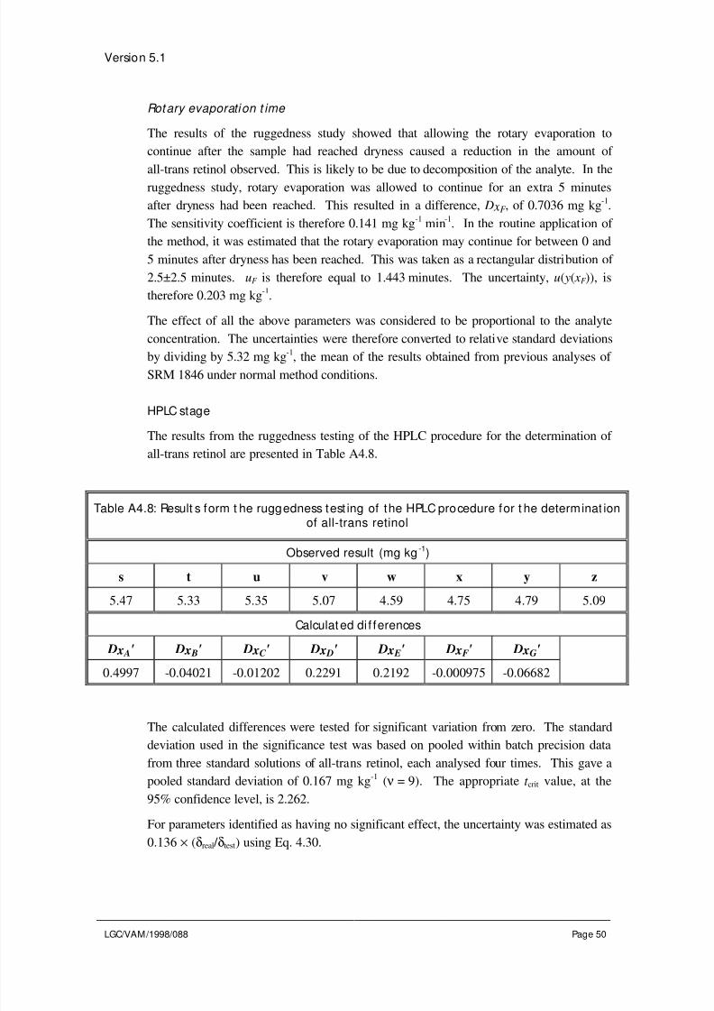
8/3/2019 At01 VAM Uncertainty
http://slidepdf.com/reader/full/at01-vam-uncertainty 53/90
Version 5.1
LGC/VAM/1998/088 Page 50
Rotary evaporation t ime
The results of the ruggedness study showed that allowing the rotary evaporation to
continue after the sample had reached dryness caused a reduction in the amount of
all-trans retinol observed. This is likely to be due to decomposition of the analyte. In the
ruggedness study, rotary evaporation was allowed to continue for an extra 5 minutes
after dryness had been reached. This resulted in a difference, D xF , of 0.7036 mg kg-1
.
The sensitivity coefficient is therefore 0.141 mg kg-1
min-1
. In the routine application of
the method, it was estimated that the rotary evaporation may continue for between 0 and
5 minutes after dryness has been reached. This was taken as a rectangular distribution of
2.5±2.5 minutes. uF is therefore equal to 1.443 minutes. The uncertainty, u( y( xF )), is
therefore 0.203 mg kg-1
.
The effect of all the above parameters was considered to be proportional to the analyte
concentration. The uncertainties were therefore converted to relative standard deviations
by dividing by 5.32 mg kg-1, the mean of the results obtained from previous analyses of
SRM 1846 under normal method conditions.
HPLC stage
The results from the ruggedness testing of the HPLC procedure for the determination of
all-trans retinol are presented in Table A4.8.
Table A4.8: Result s form t he ruggedness test ing of the HPLC procedure for t he determinat ionof all-trans retinol
Observed result (mg kg -1)
s t u v w x y z
5.47 5.33 5.35 5.07 4.59 4.75 4.79 5.09
Calculated di f ferences
D x A' D x B' D xC ' D x D' D x E' D x F' D xG'
0.4997 -0.04021 -0.01202 0.2291 0.2192 -0.000975 -0.06682
The calculated differences were tested for significant variation from zero. The standard
deviation used in the significance test was based on pooled within batch precision data
from three standard solutions of all-trans retinol, each analysed four times. This gave a
pooled standard deviation of 0.167 mg kg-1
( ν = 9). The appropriate t crit value, at the
95% confidence level, is 2.262.
For parameters identified as having no significant effect, the uncertainty was estimated as
0.136 × (δreal / δtest) using Eq. 4.30.

8/3/2019 At01 VAM Uncertainty
http://slidepdf.com/reader/full/at01-vam-uncertainty 54/90
Version 5.1
LGC/VAM/1998/088 Page 51
Flow rate
The method has been developed using a flow rate of 1 ml min-1
. Information in the
literature suggests that a typical variation in flow rate is ±0.3 %. This corresponds to
0.003 ml min-1
in this case.
δreal is therefore equal to 0.006 ml min
-1. In the ruggedness
study the flow rate was changed from 0.8 ml min-1
to 1.2 ml min-1
. δtest is therefore
0.4 ml min-1
. The uncertainty in the final result due to variations in the flow rate,
u( y( x B' )) is therefore 0.00204 mg kg-1
.
Mobile phase compositi on
The method specifies a mobile phase composition of methanol:water (90:10 v/v). From
the literature it is estimated that the variation in mixing the mobile phase is unlikely to
exceed more than ±1 % in either of the components. In the ruggedness study the
composition was changed to 95:5 (v/v) methanol:water, a much larger change than would
be expected in the normal application of the method. As a first estimate, it was assumedthat, during normal use of the method, the effect on the final result due to variations in
the mobile phase composition would be one tenth of that observed in the ruggedness test.
The uncertainty, u( y( x D' )), is therefore 0.0136 mg kg-1
.
Injection volume
Information in the literature indicates 1.5% to be a typical coefficient of variation for the
volume delivered by an auto sampler. The method specifies an injection volume of 20 µl.
δreal is therefore 0.6 µl. In the ruggedness study the injection volume was varied by 10 µl
(δtest). The uncertainty, u( y( x E ' )), is therefore 0.00816 mg kg-1
.
Detection wavelength
In the ruggedness study the detection wavelength was varied by 10 nm. Based on
information in the literature, a wavelength accuracy of ±2 nm is assumed. The
uncertainty, u( y( xF ' )), is 0.0544 mg kg-1
.
Column temperature
As part of the ruggedness study, the effect of using an un-thermostatted column was
investigated. During the study the laboratory temperature averaged at 22.2°C with a
%CV of 1%. The column is normally maintained at 30°C. It is estimated that this is
controlled to within ±1°C. δreal and δtest are therefore equal to 2°C and 7.8°Crespectively. The uncertainty, u( y( xG' )), is therefore 0.0349 mg kg
-1.
The effect of all the above parameters was considered to be proportional to the analyte
concentration. The uncertainties were therefore converted to relative standard deviations
by dividing by 5.32 mg kg-1
Only one parameter was found to be having a significant effect on the method
performance - the age of the column. A lower result was obtained when an old column
was used compared to a brand new one. Further investigation of the data revealed that
this was due to the peak area for the standard increasing on the old column, whilst the
peak area for the sample decreased, leading to a decrease in the calculated concentration.

8/3/2019 At01 VAM Uncertainty
http://slidepdf.com/reader/full/at01-vam-uncertainty 55/90
Version 5.1
LGC/VAM/1998/088 Page 52
The results of the ruggedness test indicate that as the column ages the method
performance will change. During routine application of the method this should be
monitored using an HPLC QC standard. Only when this is performing adequately (after
adjustment of the HPLC conditions if necessary) will sample extracts be presented for
analysis. Due to the relatively short timescale it is unlikely that the precision study
undertaken as part of the validation study would include variability in method
performance due to column ageing. However, when the method is in routine use a check
sample will be analysed and data collected over a period of time. The variation observed
in these results will include the variability due to changes in the column performance,
within the bounds permitted by the HPLC QC standard. If the long term precision
estimate obtained from the QC sample is significantly different from that obtained from
the precision study described earlier, then it can be used to generate a revised uncertainty
estimate at a later data. For the above reasons, an estimate of the uncertainty due to
ageing of the HPLC column has not been included in the present uncertainty budget.
Remaining sources of uncertainty
The precision and trueness studies were designed to cover as many of the sources of
uncertainty as possible (see cause and effect diagram, Figures A1.1 and A1.2), for
example, by analysing a range of concentration levels, and by preparing new standards
and HPLC mobile phase for each batch of analyses. Parameters which were not
adequately varied during these experiments, such as the extraction and HPLC conditions,
were investigated in the ruggedness tests. There are however, a small number of
parameters which were not covered by the above experiments. These generally related to
the calibration of volumetric glassware and balances used in the preparation of the
standards and samples. For example, during this study the same balance was used to
weigh out all the samples. Although the precision associated with this operation is
included in the overall precision estimate, the effect of the accuracy of the balance has
not been included in the uncertainty budget so far. The balance used in the study may
typically have a positive bias of 0.0001 g. In the future a different balance, or the same
balance after re-calibration, may have a negative bias of 0.0001 g. Since this possible
variation is not already included in the uncertainty budget it should be considered
separately. However, previous experience[18]
has shown us that uncertainties associated
with the calibration of analytical balances and volumetric glassware are generally small
compared to other sources of uncertainty such as overall precision and recovery.
Additional uncertainty estimates for these parameters have not therefore been included in
the uncertainty budget.

8/3/2019 At01 VAM Uncertainty
http://slidepdf.com/reader/full/at01-vam-uncertainty 56/90
Version 5.1
LGC/VAM/1998/088 Page 53
A4.1.5 Calculation of combined and expanded uncertainties
Table A4.9 presents the magnitudes of the individual uncertainty components for the
determination of all-trans retinol in infant formula.
Table A4.9: Uncertainty budget f or t he determination of all-trans retinolin infant f ormula
Parameter Standard uncertainty
Precision u(P) 0.238 mg kg-1
Recovery u( R) 0.0586
Weight KOH used in ethanolic KOH u( y( x A)) 0.000224
Saponification time u( y( x B)) 0.0106Shaking time for each ether extraction u( y( x D)) 0.0346
Number of water washes u( y( x E )) 0.0115
Rotary evaporation time u( y( xF )) 0.0382
Rotary evaporation temperature u( y( xG)) 0.00692
Flow rate u( y( x B' )) 0.000383
Mobile phase composition u( y( x D' )) 0.00256
Injection volume u( y( x E ' )) 0.00153
Detection wavelength u( y( xF ' )) 0.0103
Column temperature u( y( xG' )) 0.00656
Note that standard uncertainties given without units are expressed as relative
standard deviations.
The sources of uncertainty that were identified as being proportional to analyte
concentration were combined by calculating the root sum of squares as in Eq. 5.1:
u y y( ) = 0 0809.
This was combined with the uncertainty associated with method precision, which was
found to be independent of analyte concentration, using Eq. 5.3. For example, for a
sample containing 5 mg kg-1
all-trans retinol:
( )u y( )' . . .= + × =0 238 5 0 0809 0 472 2
mg kg-1
Similar calculations lead to the following estimates of uncertainty for a range of typical
all-trans retinol concentrations:

8/3/2019 At01 VAM Uncertainty
http://slidepdf.com/reader/full/at01-vam-uncertainty 57/90
Version 5.1
LGC/VAM/1998/088 Page 54
Table A4.10: Standard uncertainty estimates for the determination ofall-trans retinol in inf ant formula
Concentration(mg kg-1)
Standard uncertainty(mg kg-1)
Relative standarduncertainty
5 0.47 0.094
7.5 0.65 0.087
10 0.84 0.084
Expanded uncertainties were obtained by multiplying the standard uncertainties by a
coverage factor, k = 2, which gives a level of confidence of approximately 95%:
Table A4.11: Expanded uncertainty estimates for the determinationof all-trans retinol in infant formula
Concentration(mg kg-1)
Expandeduncertainty
(mg kg-1)
Relative expandeduncertainty
5 0.94 0.19
7.5 1.30 0.17
10 1.69 0.17
Comments on uncertaint y budget
Figure A4.2 illustrates the contributions to the measurement uncertainty for the
determination of all-trans retinol in infant formula at a concentration of 5 mg kg-1
. The
vertical line indicates one third of the magnitude of the largest contribution to the
uncertainty budget (in this case recovery). Only parameters with uncertainties greater
than this value need to be considered as significant sources of uncertainty for the method.
In this case the four major contributions were identified as precision and recovery for theentire method, and the effects of the length of time each ether extract is shaken with water
and of evaporating the ether extract to dryness. Both the latter uncertainties were
evaluated using data from the ruggedness test. The test is designed to highlight the
parameters which have a significant effect on method performance and also to give an
initial uncertainty estimate for each parameter. If the uncertainty estimate so obtained is
a significant contribution to the uncertainty estimate, ideally the effects of changes in that
parameter should be investigated further. In this case, for example, that could involve
separate studies to investigate the effect of shaking time and rotary evaporation
conditions on the result of the analysis. It will then be possible to include a refined
uncertainty estimate in the uncertainty budget. If the uncertainties associated with these

8/3/2019 At01 VAM Uncertainty
http://slidepdf.com/reader/full/at01-vam-uncertainty 58/90
Version 5.1
LGC/VAM/1998/088 Page 55
parameters are unacceptably large, the parameters will have to be more strictly controlled
in the method protocol, for example by specifying a shaking time of 2 minutes±10
seconds. If it is not possible to control the parameter sufficiently, i.e., if the control
limits required would be so tight as to be impossible to achieve during routine application
of the method, then further method development will be required.
0 0.005 0.01 0.015 0.02 0.025 0.03 0.035 0.04 0.045 0.05 0.055 0.06
Uncertainty as a relative standard deviation
Precision
Recovery
Weight KOH
Saponification time
Shaking time
No. water washes
Rotary evaporation time
Rotary evaporation temp
Flow rate
Mobile phase composition
Injection volume
Detection wavelength
Column temp
P a r a m e t e r
Figure A4.2: Cont ribut ions to t he measuremrnt uncertainty fo r t he
determination of all-trans retinol in inf ant f ormula
(analyte concentration 5 mg kg -1)
1/3rd largest uncertainty
component
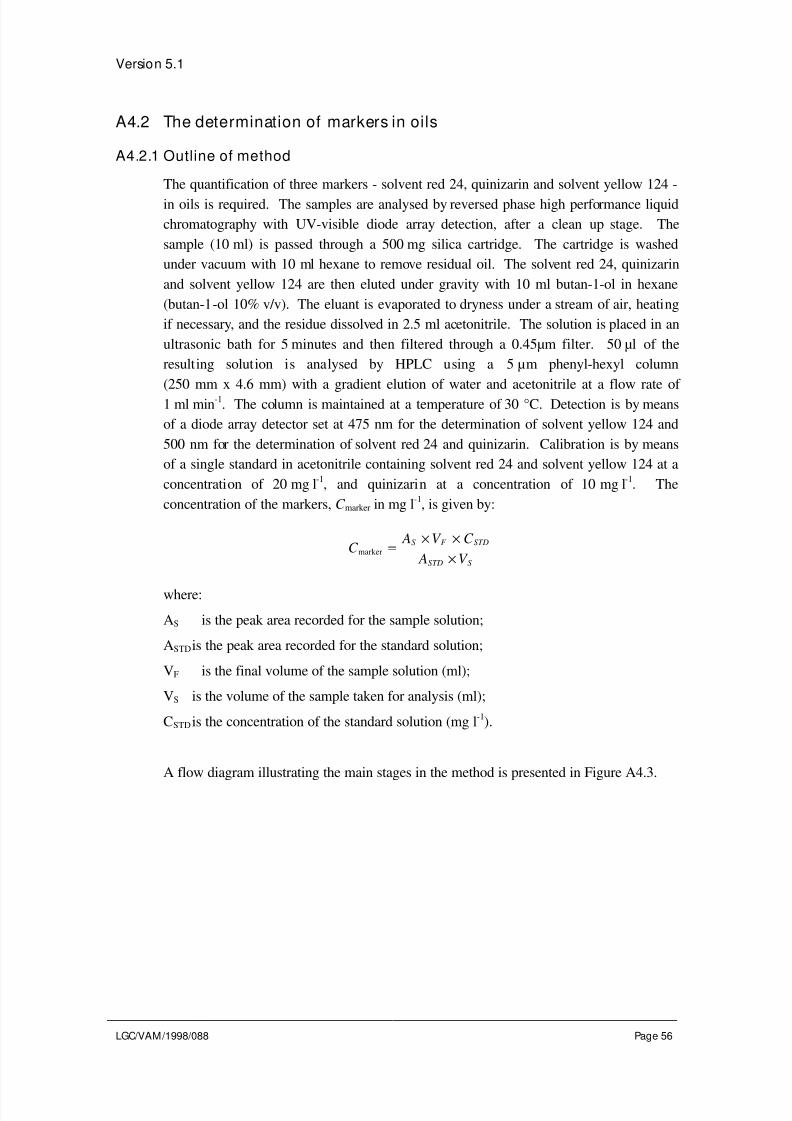
8/3/2019 At01 VAM Uncertainty
http://slidepdf.com/reader/full/at01-vam-uncertainty 59/90
Version 5.1
LGC/VAM/1998/088 Page 56
A4.2 The determination of markers in oils
A4.2.1 Outline of method
The quantification of three markers - solvent red 24, quinizarin and solvent yellow 124 -
in oils is required. The samples are analysed by reversed phase high performance liquid
chromatography with UV-visible diode array detection, after a clean up stage. The
sample (10 ml) is passed through a 500 mg silica cartridge. The cartridge is washed
under vacuum with 10 ml hexane to remove residual oil. The solvent red 24, quinizarin
and solvent yellow 124 are then eluted under gravity with 10 ml butan-1-ol in hexane
(butan-1-ol 10% v/v). The eluant is evaporated to dryness under a stream of air, heating
if necessary, and the residue dissolved in 2.5 ml acetonitrile. The solution is placed in an
ultrasonic bath for 5 minutes and then filtered through a 0.45µm filter. 50 µl of the
resulting solution is analysed by HPLC using a 5 µm phenyl-hexyl column
(250 mm x 4.6 mm) with a gradient elution of water and acetonitrile at a flow rate of
1 ml min-1
. The column is maintained at a temperature of 30 °C. Detection is by means
of a diode array detector set at 475 nm for the determination of solvent yellow 124 and
500 nm for the determination of solvent red 24 and quinizarin. Calibration is by means
of a single standard in acetonitrile containing solvent red 24 and solvent yellow 124 at a
concentration of 20 mg l-1
, and quinizarin at a concentration of 10 mg l-1
. The
concentration of the markers, C marker in mg l-1
, is given by:
C A V C
A V
S F STD
STD S
marker =× ×
×
where:
AS is the peak area recorded for the sample solution;
ASTDis the peak area recorded for the standard solution;
VF is the final volume of the sample solution (ml);
VS is the volume of the sample taken for analysis (ml);
CSTD is the concentration of the standard solution (mg l-1
).
A flow diagram illustrating the main stages in the method is presented in Figure A4.3.

8/3/2019 At01 VAM Uncertainty
http://slidepdf.com/reader/full/at01-vam-uncertainty 60/90
Version 5.1
LGC/VAM/1998/088 Page 57
Transfer 10 ml sample by pipette onto a
500 mg silica SPE cartridge
Drain under vacuum until cartridge is dry
Wash cartridge under vacuum
with 10 ml hexane
Elute markers from cartridge under gravity
with 10 ml butan-1-ol in hexane (10% v/v)
Evaporate eluant to dryness under air
stream, heating if necessary
Dissolve residue in 2.5 ml acetonitrile
Filter solution through
0.45µm filter
Quantify markers using reverse phase
HPLC with diode array detection
Figure A4.3: Flow diagram illustrating the stages in t he method f or t hedetermination of markers in diesel oil
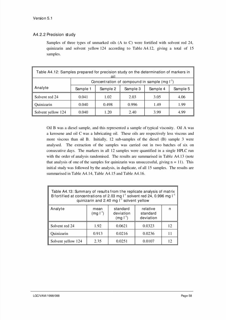
8/3/2019 At01 VAM Uncertainty
http://slidepdf.com/reader/full/at01-vam-uncertainty 61/90
Version 5.1
LGC/VAM/1998/088 Page 58
A4.2.2 Precision study
Samples of three types of unmarked oils (A to C) were fortified with solvent red 24,
quinizarin and solvent yellow 124 according to Table A4.12, giving a total of 15
samples.
Table A4.12: Samples prepared for precision study on the determination of markers inoi l
Concent ration of compound in sample (mg l-1)
Analyte Sample 1 Sample 2 Sample 3 Sample 4 Sample 5
Solvent red 24 0.041 1.02 2.03 3.05 4.06
Quinizarin 0.040 0.498 0.996 1.49 1.99
Solvent yellow 124 0.040 1.20 2.40 3.99 4.99
Oil B was a diesel sample, and this represented a sample of typical viscosity. Oil A was
a kerosene and oil C was a lubricating oil. These oils are respectively less viscous and
more viscous than oil B. Initially, 12 sub-samples of the diesel (B) sample 3 were
analysed. The extraction of the samples was carried out in two batches of six on
consecutive days. The markers in all 12 samples were quantified in a single HPLC run
with the order of analysis randomised. The results are summarised in Table A4.13 (note
that analysis of one of the samples for quinizarin was unsuccessful, giving n = 11). This
initial study was followed by the analysis, in duplicate, of all 15 samples. The results aresummarised in Table A4.14, Table A4.15 and Table A4.16.
Table A4.13: Summary of result s f rom t he replicate analysis of mat rixB fort if ied at concentrati ons of 2.03 mg l-1 solvent red 24, 0.996 mg l -1
quinizarin and 2.40 mg l-1 solvent yellow
Analyte mean(mg l-1)
standarddeviation
(mg l-1)
relativestandarddeviation
n
Solvent red 24 1.92 0.0621 0.0323 12
Quinizarin 0.913 0.0216 0.0236 11
Solvent yellow 124 2.35 0.0251 0.0107 12

8/3/2019 At01 VAM Uncertainty
http://slidepdf.com/reader/full/at01-vam-uncertainty 62/90
Version 5.1
LGC/VAM/1998/088 Page 59
Table A4.14: Summary of result s f rom t he duplicate analysis of oil samples spikedw ith solvent red 24 at a range of concentrations
Mat rix Target conc(mg l-1)
Observed conc(mg l-1)
mean Dif ference Normaliseddifference
A 0.041 0.033 0.036 0.035 -0.003 -0.0883
A 1.02 0.989 0.969 0.979 0.019 0.0199
A 2.03 1.96 1.98 1.97 -0.016 -0.00837
A 3.05 2.98 2.88 2.93 0.098 0.0334
A 4.06 3.99 4.01 4.00 -0.019 -0.00474
B 0.041 0.044 0.036 0.040 0.007 0.181
B 1.02 0.945 0.927 0.936 0.018 0.0191B 2.03 1.98 1.96 1.97 0.013 0.00669
B 3.05 2.83 2.90 2.87 -0.065 -0.0226
B 4.06 3.90 3.88 3.89 0.025 0.00650
C 0.041 0.039 0.040 0.040 -0.001 -0.0195
C 1.02 0.921 0.963 0.942 -0.043 -0.0455
C 2.03 1.93 1.87 1.90 0.064 0.0339
C 3.05 2.96 3.02 2.99 -0.061 -0.0205
C 4.03 3.92 4.04 3.98 -0.120 -0.0302
s 0.0532 0.0585
s / √2 0.0376 0.0414

8/3/2019 At01 VAM Uncertainty
http://slidepdf.com/reader/full/at01-vam-uncertainty 63/90
Version 5.1
LGC/VAM/1998/088 Page 60
Table A4.15: Summary of result s f rom t he duplicate analysis of oil samples spikedwith quinizarin at a range of concentrations
Mat rix Target conc(mg l-1)
Observed conc(mg l-1)
mean Dif ferences Normaliseddifference
A 0.040 0.030 0.029 0.030 0.001 0.0398
A 0.498 0.359 0.360 0.360 -0.002 -0.00422
A 0.996 0.743 0.700 0.722 0.042 0.0587
A 1.49 0.999 1.13 1.07 -0.135 -0.127
A 1.99 1.58 1.59 1.58 -0.013 -0.00815
B 0.040 0.030 0.027 0.029 0.003 0.100
B 0.498 0.421 0.443 0.432 -0.023 -0.0529
B 0.996 0.909 0.892 0.900 0.018 0.0196
B 1.49 1.37 1.35 1.36 0.022 0.0160
B 1.99 1.88 1.87 1.88 0.010 0.00533
C 0.040 0.034 0.031 0.032 0.003 0.0954
C 0.498 0.355 0.248 0.302 0.107 0.354
C 0.996 0.779 0.665 0.722 0.114 0.158
C 1.49 1.20 1.11 1.16 0.089 0.0769
C 1.99 1.53 1.63 1.58 -0.095 -0.0602
s 0.0664 0.111
s / √2 0.0470 0.0788
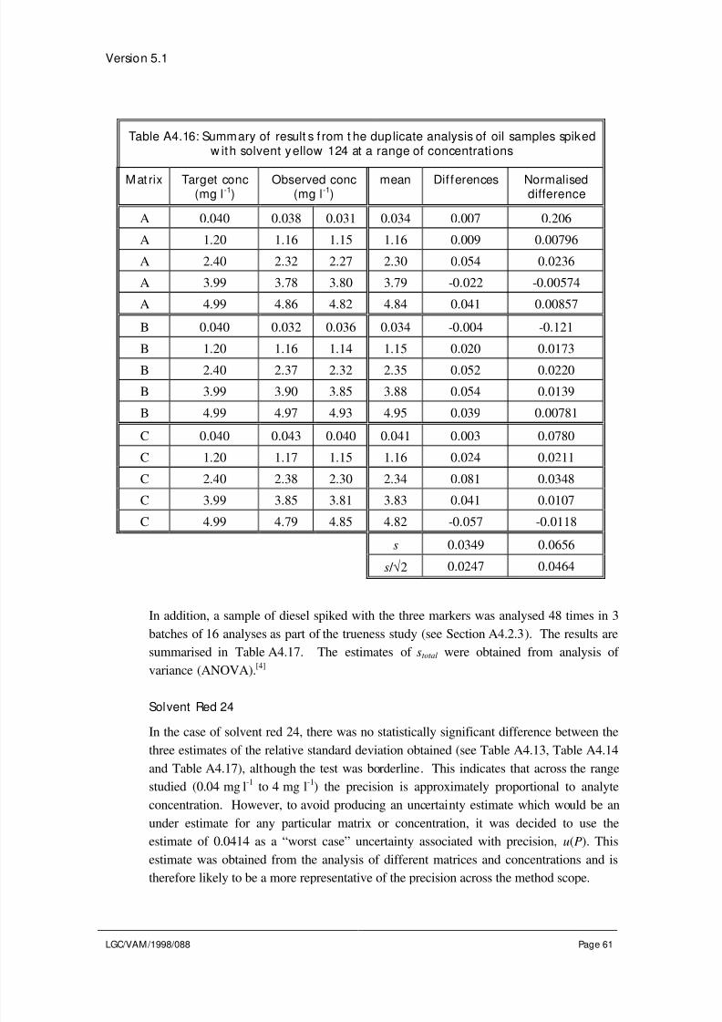
8/3/2019 At01 VAM Uncertainty
http://slidepdf.com/reader/full/at01-vam-uncertainty 64/90
Version 5.1
LGC/VAM/1998/088 Page 61
Table A4.16: Summary of result s f rom t he duplicate analysis of oil samples spikedw ith solvent yellow 124 at a range of concentrations
Mat rix Target conc(mg l-1)
Observed conc(mg l-1)
mean Dif ferences Normaliseddifference
A 0.040 0.038 0.031 0.034 0.007 0.206
A 1.20 1.16 1.15 1.16 0.009 0.00796
A 2.40 2.32 2.27 2.30 0.054 0.0236
A 3.99 3.78 3.80 3.79 -0.022 -0.00574
A 4.99 4.86 4.82 4.84 0.041 0.00857
B 0.040 0.032 0.036 0.034 -0.004 -0.121
B 1.20 1.16 1.14 1.15 0.020 0.0173
B 2.40 2.37 2.32 2.35 0.052 0.0220
B 3.99 3.90 3.85 3.88 0.054 0.0139
B 4.99 4.97 4.93 4.95 0.039 0.00781
C 0.040 0.043 0.040 0.041 0.003 0.0780
C 1.20 1.17 1.15 1.16 0.024 0.0211
C 2.40 2.38 2.30 2.34 0.081 0.0348
C 3.99 3.85 3.81 3.83 0.041 0.0107
C 4.99 4.79 4.85 4.82 -0.057 -0.0118
s 0.0349 0.0656
s / √2 0.0247 0.0464
In addition, a sample of diesel spiked with the three markers was analysed 48 times in 3
batches of 16 analyses as part of the trueness study (see Section A4.2.3). The results are
summarised in Table A4.17. The estimates of stotal were obtained from analysis of
variance (ANOVA).[4]
Solvent Red 24
In the case of solvent red 24, there was no statistically significant difference between the
three estimates of the relative standard deviation obtained (see Table A4.13, Table A4.14
and Table A4.17), although the test was borderline. This indicates that across the range
studied (0.04 mg l-1
to 4 mg l-1
) the precision is approximately proportional to analyte
concentration. However, to avoid producing an uncertainty estimate which would be an
under estimate for any particular matrix or concentration, it was decided to use the
estimate of 0.0414 as a “worst case” uncertainty associated with precision, u(P). This
estimate was obtained from the analysis of different matrices and concentrations and is
therefore likely to be a more representative of the precision across the method scope.
8/3/2019 At01 VAM Uncertainty
http://slidepdf.com/reader/full/at01-vam-uncertainty 65/90
Version 5.1
LGC/VAM/1998/088 Page 62
Quinizarin
The various estimates of the standard deviation and relative standard deviation were not
comparable. In particular, the estimates obtained from the duplicate results were
significantly different from the other estimates. However, there were no obvious patterns
in the data so no particular matrix and/or concentration could be identified as being the
cause of the variability. There was therefore no justification for removing any data and
restricting the coverage of the uncertainty estimate, as in the case of solvent yellow 124
(see below). The results of the precision studies indicate that the method is more variable
across different matrices and analyte concentrations for quinizarin than for the other
markers. The uncertainty associated with the precision was therefore taken as the
estimate of the relative standard deviation obtained from the duplicate results, 0.0788.
This represents a worst case estimate but it should ensure that the uncertainty is not
underestimated for any given matrix or concentration (although it may result in an
overestimate in some cases).
Solvent yellow 124
There was no significant difference between the estimates of the relative standard
deviation obtained for samples at concentrations of 2.4 mg l-1
and 4.99 mg l-1
. However,
the estimate obtained from the duplicate analyses was significantly greater than the other
estimates. Inspection of that data revealed that the normalised differences observed for
the samples at a concentration of 0.04 mg l-1
were substantially larger than those
observed at the other concentrations. Removing these data points gave a revised estimate
of the relative standard deviation of 0.00903. This was in agreement with the other
estimates obtained (F-tests, 95% confidence). The three estimates were therefore pooled
using Eq. 4.2 to give a single estimate of the relative standard deviation of 0.0114. As it
stands, the uncertainty estimate cannot be applied to samples with concentrations below
1.2 mg l-1
. Further study would be required to investigate in more detail the precision at
these low levels.
A4.2.3 Trueness study
Calculation of R m and u( R m )
In this case there was no suitable CRM available for the evaluation of Rm . The best
option available was to use spiked samples. In this example, the behaviour of spiked
samples is likely to be a good representation of that of test samples, as oils are marked
simply by adding and mixing in the required amount of the markers. A 2000 ml sample
of unmarked BP diesel was spiked with standards in toluene containing solvent red 24,
quinizarin and solvent yellow 124 at concentrations of 0.996 mg ml-1
, 1.02 mg ml-1
and
1.97 mg ml-1
respectively to give concentrations in the diesel of 4.06 mg l-1
, 1.99 mg l-1
and 4.99 mg l-1
respectively. Forty-eight aliquots of this sample were analysed in three
batches of 16 analyses. The results are summarised in Table A4.17.

8/3/2019 At01 VAM Uncertainty
http://slidepdf.com/reader/full/at01-vam-uncertainty 66/90
Version 5.1
LGC/VAM/1998/088 Page 63
Table A4.17: Result s f rom the replicate analysis of a diesel oil spiked w ith solvent red 24,quinizarin and solvent yellow 124
Analyte Target
concentrationC spike
(mg l-1)
Mean
C obs
(mg l-1)
Standard
deviation ofthe mean,
s mean
(mg l-1)a
Total
standarddeviation,
s total (mg l-1)b
Relative
standarddeviation
Solvent red 24 4.06 3.88 0.0360 0.112 0.0289
Quinizarin 1.99 1.89 0.00370 0.0256 0.0136
Solvent yellow 124 4.99 4.99 0.0167 0.0618 0.0124
aEstimated from ANOVA of 3 groups of 16 replicates according to ISO 5725:1994
[19]
bEstimated from ANOVA
[4]
Rm
was calculated as described in Section 4.2.2.1. The mean recovery and its
uncertainty were calculated using Eq. 4.5 and Eq. 4.6 respectively, where smean given in
Table A4.17 is equivalent to sobs / √n.
For solvent red 24:
Rm = =388 4 06 0 956. / . .
Based on information on the purity of the material used to prepare the spiked sample, and
the accuracy and precision of volumetric glassware and analytical balances used, the
uncertainty in the concentration of solvent red 24 in the sample, u(C spike), was estimated
as 0.05 mg l-1
.**
The uncertainty in Rm
is therefore given by:
u Rm( ) = ×
+
=0956
0 0360
388
0 05
4 0600148
2 2
..
.
.
..
The uncertainties associated with the concentration of quinizarin and solvent yellow 124
in the spiked sample were estimated as 0.025 mg l-1
and 0.062 mg l-1
respectively.
Similar calculations as above for quinizarin and solvent yellow 124 produced the
following estimates:
quinizarin: Rm
= 0.949, u Rm
( ) = 0.0121
solvent yellow 124, Rm
= 1.00, u Rm
( ) = 0.0129
To determine the contribution of Rm
to the combined uncertainty, the value calculated
above was compared with 1, using Eq. 4.18. For solvent red 24:
**Detailed information on the estimation of uncertainties of this type is presented in reference 2
8/3/2019 At01 VAM Uncertainty
http://slidepdf.com/reader/full/at01-vam-uncertainty 67/90
Version 5.1
LGC/VAM/1998/088 Page 64
t =−
=1 0 956
0 01482 97
.
..
In this case, t was compared with coverage factor, k = 2. A t value greater than two
suggests that Rm is significantly different from 1. However, in the normal application of the method, no correction will be made to take account of the fact that the method
recovery is significantly different from 1. This is an example of case 3 discussed in
Section 4.2.5. Accordingly, Eq. 4.20 was used to calculate the uncertainty u Rm
( )' ' :
u Rm( )' ' =−
+ =
1 0 956
20 0148 0 0262
2
2.. .
The significance test also indicated that the recovery of quinizarin was significantly
different from 1. Applying Eq. 4.20 gives a value of u Rm
( )'' of 0.0283. In the case of
solvent yellow 124, the significance test indicated that Rm was not significantly different
from 1. This is an example of case 1 discussed in Section 4.2.5. In such cases the
uncertainty associated with Rm
is the value of u Rm
( ) calculated above (i.e., 0.0129).
Calculation of R s
Rs was calculated using the results from the samples analysed in the precision study and
the data from the determination of Rm
. u( Rs) is the standard deviation of the mean
recoveries obtained for the different matrices and analyte concentrations. The data are
summarised in Table A4.18 to Table A4.20.
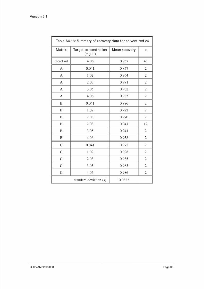
8/3/2019 At01 VAM Uncertainty
http://slidepdf.com/reader/full/at01-vam-uncertainty 68/90
Version 5.1
LGC/VAM/1998/088 Page 65
Table A4.18: Summary of recovery data for solvent red 24
Matrix Target concent rat ion(mg l-1)
Mean recovery n
diesel oil 4.06 0.957 48
A 0.041 0.857 2
A 1.02 0.964 2
A 2.03 0.971 2
A 3.05 0.962 2
A 4.06 0.985 2
B 0.041 0.986 2
B 1.02 0.922 2
B 2.03 0.970 2
B 2.03 0.947 12
B 3.05 0.941 2
B 4.06 0.958 2
C 0.041 0.975 2
C 1.02 0.928 2
C 2.03 0.935 2
C 3.05 0.983 2
C 4.06 0.986 2
standard deviation (s) 0.0322
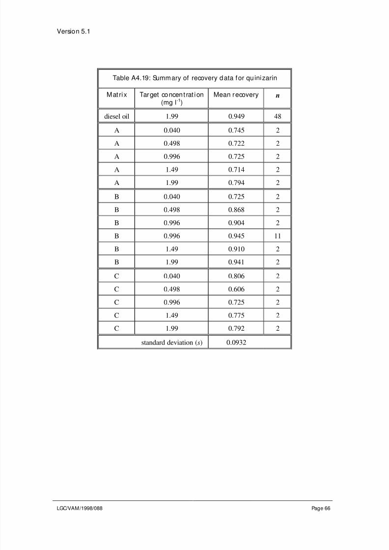
8/3/2019 At01 VAM Uncertainty
http://slidepdf.com/reader/full/at01-vam-uncertainty 69/90
Version 5.1
LGC/VAM/1998/088 Page 66
Table A4.19: Summary of recovery data for qu inizarin
Matrix Target concent rat ion(mg l-1)
Mean recovery n
diesel oil 1.99 0.949 48
A 0.040 0.745 2
A 0.498 0.722 2
A 0.996 0.725 2
A 1.49 0.714 2
A 1.99 0.794 2
B 0.040 0.725 2
B 0.498 0.868 2
B 0.996 0.904 2
B 0.996 0.945 11
B 1.49 0.910 2
B 1.99 0.941 2
C 0.040 0.806 2
C 0.498 0.606 2
C 0.996 0.725 2
C 1.49 0.775 2
C 1.99 0.792 2
standard deviation (s) 0.0932

8/3/2019 At01 VAM Uncertainty
http://slidepdf.com/reader/full/at01-vam-uncertainty 70/90
Version 5.1
LGC/VAM/1998/088 Page 67
Table A4.20: Summary of recovery data f orsolvent yellow 124
Matrix Target concent rat ion(mg l-1)
Mean recovery n
diesel oil 4.99 1.00 48
A 0.040 0.857 2
A 1.20 0.966 2
A 2.40 0.959 2
A 3.99 0.949 2
A 4.99 0.970 2
B 0.040 0.841 2
B 1.20 0.957 2
B 2.40 0.979 2
B 2.40 0.978 12
B 3.99 0.971 2
B 4.99 0.992 2
C 0.040 1.04 2
C 1.20 0.969 2
C 2.40 0.977 2
C 3.99 0.958 2
C 4.99 0.966 2
standard deviation (s) 0.0426
s excluding recoveries at 0.04 mg l-1
0.0138
For solvent red 24, the standard deviation of the mean recoveries obtained at variousconcentrations and from various matrices was calculated as 0.0322. As discussed in
Section 4.2.6, this was used as the estimate of u( Rs).
In the case of quinizarin, the standard deviation of the mean recoveries was 0.0932. The
large standard deviation is due to the fact that the recoveries obtained for matrix B were
generally higher than those obtained for matrices A or C. In this example, a single
uncertainty estimate will be reported for all the matrices studied. However, if this
estimate was found to be unsatisfactory for future applications of the method, separate
budgets could be calculated for individual matrices.
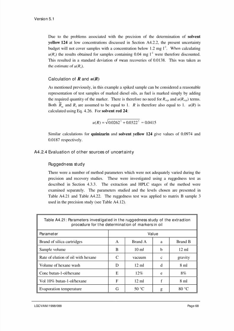
8/3/2019 At01 VAM Uncertainty
http://slidepdf.com/reader/full/at01-vam-uncertainty 71/90
Version 5.1
LGC/VAM/1998/088 Page 68
Due to the problems associated with the precision of the determination of solvent
yellow 124 at low concentrations discussed in Section A4.2.2, the present uncertainty
budget will not cover samples with a concentration below 1.2 mg l-1
. When calculating
u( Rs) the results obtained for samples containing 0.04 mg l-1
were therefore discounted.
This resulted in a standard deviation of mean recoveries of 0.0138. This was taken as
the estimate of u( Rs).
Calculation of R and u( R)
As mentioned previously, in this example a spiked sample can be considered a reasonable
representation of test samples of marked diesel oils, as fuel is marked simply by adding
the required quantity of the marker. There is therefore no need for Rrep and u( Rrep) terms.
Both Rm
and Rs are assumed to be equal to 1. R is therefore also equal to 1. u( R) is
calculated using Eq. 4.26. For solvent red 24:
u R( ) = + =0 0262 0 0322 0 04152 2. . .
Similar calculations for quinizarin and solvent yellow 124 give values of 0.0974 and
0.0187 respectively.
A4.2.4 Evaluation of o ther sources of uncertainty
Ruggedness study
There were a number of method parameters which were not adequately varied during theprecision and recovery studies. These were investigated using a ruggedness test as
described in Section 4.3.3. The extraction and HPLC stages of the method were
examined separately. The parameters studied and the levels chosen are presented in
Table A4.21 and Table A4.22. The ruggedness test was applied to matrix B sample 3
used in the precision study (see Table A4.12).
Table A4.21: Parameters invest igated in t he ruggedness study of the extract ionprocedure for t he determinat ion of markers in oil
Parameter Value
Brand of silica cartridges A Brand A a Brand B
Sample volume B 10 ml b 12 ml
Rate of elution of oil with hexane C vacuum c gravity
Volume of hexane wash D 12 ml d 8 ml
Conc butan-1-ol/hexane E 12% e 8%
Vol 10% butan-1-ol/hexane F 12 ml f 8 ml
Evaporation temperature G 50 °C g 80 °C

8/3/2019 At01 VAM Uncertainty
http://slidepdf.com/reader/full/at01-vam-uncertainty 72/90
Version 5.1
LGC/VAM/1998/088 Page 69
Table A4.22: Parameters investigated in t he ruggedness study of the HPLCprocedure for t he determinat ion of markers in oil
Parameter Value
Grade of acetonitrile in mobile phase A' Far UV a' HPLC
Flow rate B' 0.8 ml min-1
b' 1.2 ml min-1
Injection volume C' 40 µl c' 60 µl
Column temperature D' 25 °C d' 35 °C
Detector wavelength (A) E' 465 nm e' 485 nm
Mobile phase degassing F' degassed f' not degassed
Detector wavelength (B) G' 490 nm g' 510 nm
Results
The results from the ruggedness studies were evaluated as described in Section 4.3.3.
Extraction stage
The results obtained from the ruggedness testing of the extraction procedure for solvent
red 24, quinizarin and solvent yellow 124 are presented in Table A4.23. The differences
for each parameter, D x A to D xG were calculated as described in Section 4.3.3.1.

8/3/2019 At01 VAM Uncertainty
http://slidepdf.com/reader/full/at01-vam-uncertainty 73/90
Version 5.1
LGC/VAM/1998/088 Page 70
Table A4.23: Results form the ruggedness testing of the extraction of solvent red 24,quinizarin and solvent yellow 124 from fuel
Solvent red 24
Observed result (mg l -1)
s t u v w x y z
2.02 2.00 2.12 2.17 1.87 1.71 2.34 2.36
Calculated di f ferences
D x A D x B D xC D x D D x E D x F D xG
0.0075 -0.3525 0.0275 0.2125 -0.0425 0.0625 -0.0275
Quinizarin
Observed result (mg l -1)
s t u v w x y z
1.10 1.06 1.15 1.01 0.96 0.86 1.28 1.26
Calculated di f ferences
D x A D x B D xC D x D D x E D x F D xG
-0.0075 -0.18 0.07 0.1775 0.0175 -0.005 -0.0425
Solvent yellow 124 (mg l-1)
Observed result
s t u v w x y z
2.41 2.38 2.52 2.66 2.19 2.15 2.76 2.87
Calculated di f ferences
D x A D x B D xC D x D D x E D x F D xG
-0.0025 -0.4225 -0.02 0.225 -0.01 0.08 0.0075
The precision of the method for the analysis of the sample used in the ruggedness studyhad previously been estimated as:
solvent red 24: 0.0621 mg l-1
( ν = 11)
quinizarin: 0.0216 mg l-1
( ν = 10)
solvent yellow 124: 0.0251 mg l-1
( ν = 11)
Using Eq. 4.29, t values were calculated for each parameter and each analyte. These
were compared with the appropriate critical values of t at 95% confidence (t crit = 2.201
for solvent red 24 and solvent yellow 124, and 2.228 for quinizarin).
8/3/2019 At01 VAM Uncertainty
http://slidepdf.com/reader/full/at01-vam-uncertainty 74/90
Version 5.1
LGC/VAM/1998/088 Page 71
Solvent red 24
In cases were the effect of a parameter was found not to be significant, Eq. 4.30 was
used to calculate the uncertainty:
u y xireal
test
real
test
( ( )) =× ×
×× = ×
2 2 201 0 0621
4 1960 0493
. .
..
δδ
δδ
Brand of sil ica cart ridge
The ruggedness test investigated the effect of changing between brands of silica cartridge.
Since this is likely to happen during the routine application of the method, δreal can be
considered as being equal to δtest. The uncertainty, u( y( x A)), is therefore 0.0493 mg l-1
.
Rate of elution of oil w ith hexane
The effect of the rate of elution of oil by hexane from the cartridge was investigated by
comparing the difference between elution under a vacuum and elution under gravity.
When the method is used routinely, the oil will be eluted under vacuum. Variations in the
vacuum applied from one extraction to another will affect the rate of elution of the oil
and the amount of oil eluted. However, the effect of variations in the vacuum will be
small compared to the effect of having no vacuum present. It can therefore be assumed
that variations in the observed concentration of the markers, due to variability in the
vacuum, will be small compared to the differences observed in the ruggedness test. As a
first estimate, the effect of variation in the vacuum during routine application of the
method was estimated as one tenth of that observed during the ruggedness study.
Concentration of butan-1-ol in hexane
The method was developed using a concentration of 10% (v/v) butan-1-ol in hexane.
Based on the manufacturers’ specification and typical precision data for the volumetric
glassware used to prepare the solution, it was estimated that the concentration may vary
by ±0.1% (v/v), i.e., δreal is 0.2% (v/v). From the ruggedness test, δtest is equal to
4% (v/v). The uncertainty, u( y( x E )), is therefore 0.00247 mg l-1.
Volume of 10% (v/v) butan-1-ol in hexane
The method was developed using 10 ml of 10% (v/v) butan-1-ol in hexane for elution of
the markers. The likely variation in this volume was estimated as ±0.04 ml (based on the
manufacturer’s specification for the pipette and typical precision data for pipettes of this
type). In the ruggedness test, the volume was changed by 4 ml. δreal and δtest are therefore
equal to 0.08 ml and 4 ml respectively. The uncertainty, u( y( xF )), is therefore
0.000986 mg l-1
.

8/3/2019 At01 VAM Uncertainty
http://slidepdf.com/reader/full/at01-vam-uncertainty 75/90
Version 5.1
LGC/VAM/1998/088 Page 72
Evaporation temperature
The method currently specifies that samples are evaporated to dryness at 50°C. The
uncertainty in this value during routine use of the method was estimated as ±5°C. δreal is
therefore 10°C.
δtest was 30°C. The uncertainty u(y( xG)) is therefore 0.0164 mg l
-1.
For parameters identified as having a significant effect on the extraction, the procedure
described in Section 4.3.3.3 was followed.
Sample volume
In the routine application of the method, 10 ml of sample is taken for analysis using an
automatic pipette. The uncertainty associated with this volume was estimated as
0.04 ml. In the ruggedness test, the volume was increased to 12 ml. This resulted in a
difference, D B, of -0.3525 mg l-1
. The sensitivity coefficient, c B, is therefore
0.1763 mg l-1
ml-1
. The uncertainty, u( y( x B)), was therefore calculated as 0.00705 mg l-1
.
Volume of hexane wash
The method was developed using 10 ml hexane (added by pipette) to wash the silica
cartridge. The uncertainty associated with the volume delivered was estimated as
0.04 ml. This is u( x D). Eq. 4.31 was used to calculate the sensitivity coefficient, c D:
c D = =02125
40 05313
.. mg l
-1ml
-1
The uncertainty in the final result due to variation in parameter D, u( y( x D)) was
calculated using Eq. 4.32:
u y x D( ( )) . . .= × =0 04 0 05313 0 00213 mg l -1
The effect of all these parameters was considered to be proportional to the analyte
concentration. The uncertainty was therefore converted to a relative standard deviation
by dividing by, 1.92 mg l-1
, the mean of the results obtained from previous analyses of
the sample under normal method conditions.
Quinizarin
For the parameters identified as not having a significant effect on the method
performance, u( y( xi)) was calculated as 0.0174 × (δreal / δtest) using Eq. 4.30. The
uncertainties were converted to relative standard deviations by dividing by 0.909 mg l-1
.
Brand of sil ica cart ridge
Using the same arguments applied in the case of solvent red 24, the uncertainty was
calculated as 0.0174 mg l-1
.
Concentration of butan-1-ol in hexane
8/3/2019 At01 VAM Uncertainty
http://slidepdf.com/reader/full/at01-vam-uncertainty 76/90
Version 5.1
LGC/VAM/1998/088 Page 73
Again applying the same reasoning as in the case of solvent red 24, the uncertainty was
estimated as 0.000868 mg l-1
.
Volume of 10% (v/v) butan-1-ol in hexane
The uncertainty was calculated as 0.000347 mg l-1, as discussed previously.
For the parameters identified as being significant, the following uncertainty estimates
were calculated:
Sample volume
The uncertainty was calculated as 0.00360 mg l-1
, using the same reasoning as applied to
solvent red 24.
Rate of elution of oil w ith hexane
As discussed above, the effect on the final result of variations in the vacuum when eluting
the oil from the cartridge with hexane was estimated as one tenth that observed in the
ruggedness test. The uncertainty, u( y( xC )) was therefore estimated as 0.0070 mg l-1
.
Volume of hexane wash
The uncertainty was evaluated as described in the case of solvent red 24. This resulted in
an uncertainty of 0.00177 mg l-1
.
Evaporation temperature
The uncertainty in the evaporation temperature was based on the assumption that the
temperature could be controlled to ±5 °C. This was taken as a rectangular distribution
and converted to a standard uncertainty by dividing by √3. The uncertainty u( y( xG)) is
therefore 0.00409 mg l-1
.
Solvent yellow 124
For the parameters identified as not having a significant effect on the method
performance, u( y( xi)) was calculated as 0.0199 × (δreal / δtest) using Eq. 4.30. The
uncertainties were converted to relative standard deviations by dividing by 2.35 mg l-1
.
Brand of sil ica cart ridge
Using the same arguments applied in the case of solvent red 24, the uncertainty was
calculated as 0.0199 mg l-1
.
Rate of elution of oil w ith hexane
This was treated as for solvent red 24, giving an uncertainty of 0.00199 mg l-1
.
Concentration of butan-1-ol in hexane
Again applying the same reasoning as in the case of solvent red 24, the uncertainty was
estimated as 0.0010 mg l-1.

8/3/2019 At01 VAM Uncertainty
http://slidepdf.com/reader/full/at01-vam-uncertainty 77/90
Version 5.1
LGC/VAM/1998/088 Page 74
Evaporation temperature
The uncertainty was calculated as 0.00663 mg l-1
, following the reasoning given for
solvent red 24.
For the parameters identified as being significant, the following uncertainty estimates
were calculated:
Sample volume
The uncertainty was calculated as 0.00845 mg l-1
, using the same reasoning as applied to
solvent red 24.
Volume of hexane wash
As for the other two markers, the volume of the hexane wash clearly influences the
recovery of solvent yellow 124. Using the procedure described for solvent red 24, the
uncertainty u( y( x D)) was calculated as 0.00225 mg l-1
.
Volume of 10% (v/v) butan-1-ol in hexane
The results indicate that the volume of butan-1-ol/hexane used to elute the marker has a
significant effect on recovery. As in the case of the hexane wash, the solution was added
by automatic pipette. The uncertainty u( y( xF )) was therefore calculated in the same way.
u( y( xF )) is therefore equal to 0.00080 mg l-1
.
HPLC stage
The results obtained from the ruggedness testing of the HPLC procedure for solvent
red 24, quinizarin and solvent yellow 124 are presented in Table A4.24. The differences
for each parameter, D x A' to D xG' were calculated as described in Section 4.3.3.1.

8/3/2019 At01 VAM Uncertainty
http://slidepdf.com/reader/full/at01-vam-uncertainty 78/90
Version 5.1
LGC/VAM/1998/088 Page 75
Table A4.24: Result s form t he ruggedness test ing of the HPLC procedure for t hedetermination of solvent red 24, quinizarin and solvent yellow 124 in fuel
Solvent red 24
Observed result (mg l -1)
s t u v w x y z
1.82 1.39 1.87 1.86 1.82 1.81 1.81 1.80
Calculated di f ferences
D x A' D x B' D xC ' D x D' D x E' D x F' D xG'
-0.0748 -0.1236 0.1152 -0.1303 0.1036 0.1082 0.1047
QuinizarinObserved result (mg l -1)
s t u v w x y z
0.947 0.911 0.846 0.915 1.02 1.00 0.932 1.07
Calculated di f ferences
D x A' D x B' D xC ' D x D' D x E' D x F' D xG'
-0.1014 0.0283 -0.0406 0.0201 0.0239 0.0641 -0.0112
Solvent yellow 124
Observed result (mg l -1)
s t u v w x y z
1.87 1.83 1.89 1.91 1.89 1.86 1.95 1.89
Calculated di f ferences
D x A' D x B' D xC ' D x D' D x E' D x F' D xG'
-0.0228 -0.0465 0.0284 -0.0023 -0.0161 0.0091 0.0198
Previous replicate analyses of a standard solution of the three markers gave the followingestimates of the precision of the HPLC system:
solvent red 24: 0.0363 mg l-1
(n = 69)
quinizarin: 0.0107 mg l-1
(n = 69)
solvent yellow 124: 0.0196 mg l-1
(n = 69)
Using Eq. 4.29, t values were calculated for each parameter and each analyte. These
were compared with the appropriate critical value of t at 95% confidence (t crit = 1.995,
ν = 68).

8/3/2019 At01 VAM Uncertainty
http://slidepdf.com/reader/full/at01-vam-uncertainty 79/90
Version 5.1
LGC/VAM/1998/088 Page 76
Solvent red 24
All the parameters studied had a significant effect on the concentration of solvent red 24
observed. The relevant uncertainties were calculated using the procedure outlined in
Section 4.3.3.3.
Flow rate
In the ruggedness test the flow rate was varied by 0.4 ml min-1. This resulted in a
difference of -0.1236 mg l-1
. The sensitivity coefficient, c B' , is therefore 0.309. The
uncertainty in the flow rate was estimated as 0.00173 ml min-1
(see section on all-trans
retinol ruggedness test). The uncertainty, u( y( x B' )), is therefore 0.000535 mg l-1
.
Injection volume
The method specifies an injection volume of 50 µl. The uncertainty associated with this
was estimated as 0.75 µl (see all-trans retinol ruggedness test). The sensitivitycoefficient, cC ' , was calculated as 0.00576. The uncertainty, u( y( xC ' )), is therefore
0.00432 mg l-1.
Column temperature
During routine use of the method, the column is thermostatted at 30°C. The uncertainty
associated with this was estimated as ±1°C (see section on all-trans retinol ruggedness
test). In the ruggedness test the temperature was varied from 25°C to 35°C which
resulted in a difference of 0.1303 mg l-1
. The sensitivity coefficient is therefore 0.01303
and the uncertainty, u( y( x D' )), is 0.00752 mg l-1
.
Channel A wavelength
The wavelength for detector channel A is specified in the method as 475 nm. The
uncertainty associated with this was estimated as ±2 nm (assuming a rectangular
distribution). In the ruggedness study, a change in wavelength of 20 nm resulted in a
difference of 0.1036 mg l-1
. The uncertainty, u( y( x E ' )), is therefore 0.00598 mg l-1.
Channel B wavelength
The wavelength for detector channel B is specified in the method as 500 nm. In the
ruggedness study a change of 20 nm resulted in a difference of 0.1047 mg l-1
. The
uncertainty is therefore 0.00604 mg l-1.
All the above uncertainties were converted to relative standard deviations by dividing by
1.92 mg l-1
.
Two other parameters also had a significant effect on the method performance: the type
of acetonitrile used in the mobile phase and whether or not the mobile phase was
degassed. The method was developed using HPLC grade acetonitrile. The ruggedness
test indicated that changing to far-UV grade results in a lower recovery. The method

8/3/2019 At01 VAM Uncertainty
http://slidepdf.com/reader/full/at01-vam-uncertainty 80/90
Version 5.1
LGC/VAM/1998/088 Page 77
protocol will therefore specify that for routine use, HPLC grade must be used. The
ruggedness test also indicated that not degassing the mobile phase causes a reduction in
recovery. The method was developed using degassed mobile phase, and the method
protocol will specify that this must be the case during future use of the method. As these
two parameters are being controlled in the method protocol, uncertainty terms have not
been included.
Quinizarin
The results of the ruggedness test indicated that the following parameters have a
significant effect on the method performance:
Flow rate
Using the procedure discussed in the case of solvent red 24, the uncertainty was
calculated as 0.000122 mg l-1
.
Injection volume
The uncertainty was calculated as 0.00152 mg l-1
(see solvent red 24 example).
Column temperature
The uncertainty was calculated as 0.00116 mg l-1
(see solvent red 24 example).
Channel A wavelength
Following the solvent red 24 example, the uncertainty was calculated as 0.00138 mg l-1
.
As in the case of solvent red 24, no additional uncertainties associated with the grade of
acetonitrile used and the degassing of the mobile phase were included.
Channel B wavelength
The ruggedness test indicated that this parameter does not have a significant effect on the
result of the analysis. The uncertainty was therefore evaluated using Eq. 4.30. δreal and
δtest are equal to 4 nm and 20 nm respectively. The uncertainty was therefore calculated
as 0.00154 mg l-1
.
All the uncertainties were converted to relative standard deviations by dividing by
0.909 mg l-1
.

8/3/2019 At01 VAM Uncertainty
http://slidepdf.com/reader/full/at01-vam-uncertainty 81/90
Version 5.1
LGC/VAM/1998/088 Page 78
Solvent yellow 124
The results of the ruggedness test indicated that the following parameters have a
significant effect on the method performance:
Flow rate
The uncertainty was calculated as 0.00020 mg l-1
(see solvent red 24 example).
Injection volume
The uncertainty was calculated as 0.00107 mg l-1
(see solvent red 24 example).
As in the case of solvent red 24 and quinizarin, no additional uncertainties associated
with the grade of acetonitrile used and the degassing of the mobile phase were included.
The results of the study indicated that remaining parameters do not have a significant
effect on the method performance. The uncertainty was therefore calculated using
Eq. 4.30 which gives 0.0141 × (δtrue / δtest).
Column temperature
δtrue and δtest are equal to 2°C and 10°C respectively. The uncertainty is therefore
0.00282 mg l-1.
Channel A wavelength
δtrue and δtest are equal to 4 nm and 20 nm respectively. The uncertainty is therefore
0.00282 mg l-1.
Channel B wavelength
As in the case of the channel A wavelength, the uncertainty was calculated as
0.00282 mg l-1.
The above uncertainties were converted to relative standard deviations by dividing by
2.35 mg l-1
.
Remaining sources of uncertainty
As discussed in Section A4.1.4 the uncertainties associated with a number of parameters,
such as the calibration of the pipette used to dispense the samples, have not yet been
considered. However, as these uncertainties are generally small, no additional
contributions to the uncertainty budget have been included.

8/3/2019 At01 VAM Uncertainty
http://slidepdf.com/reader/full/at01-vam-uncertainty 82/90
Version 5.1
LGC/VAM/1998/088 Page 79
A4.2.5 Calculation of combined and expanded uncertainties
Table A4.25 summarises the magnitudes of the individual uncertainty components for the three
makers.
Table A4.25: Uncertainty budget f or t he determination of markers in oi l
Standard uncertainties as relative standard deviations
Parameter Solvent red 24
(0.04 - 4 mg l -1)Quinizarin
(0.04 - 2 mg l -1)Solvent yellow(1.2 - 5 mg l-1)
Precision u(P) 0.0414 0.0788 0.0114
Recovery u( R) 0.0415 0.0974 0.0187
Brand of cartridge u( y( x A)) 0.0257 0.0190 0.00848
Sample volume u( y( x B)) 0.00367 0.00394 0.00360
Rate of elution of oil
with hexane
u( y( xC )) 0.00257 0.00767 0.000848
Volume of hexane wash u( y( x D)) 0.00111 0.00195 0.000957
Concentration of
butan-1-ol/hexane
u( y( x E )) 0.00128 0.000951 0.000424
Volume of
butan-1-ol/hexane
u( y( xF )) 0.000514 0.000380 0.000340
Evaporation
temperature
u( y( xG)) 0.00856 0.00480 0.00283
Flow rate u( y( x B' )) 0.000279 0.000134 0.000855
Injection volume u( y( xC ' )) 0.00225 0.00167 0.000455
Column temperature u( y( x D' )) 0.00392 0.00128 0.00120
Detector channel A
wavelength
u( y( x E ' )) 0.00311 0.00152 0.00120
Detector channel B
wavelength
u( y( xG' )) 0.00315 0.00169 0.00120
For all three analytes, the sources of uncertainty were considered to be proportional to
analyte concentration. The combined uncertainty was therefore calculated using Eq. 5.1:
solvent red 24: u( y)/ y = 0.065
quinizarin: u( y)/ y = 0.13
solvent yellow 124: u( y)/ y = 0.024

8/3/2019 At01 VAM Uncertainty
http://slidepdf.com/reader/full/at01-vam-uncertainty 83/90
Version 5.1
LGC/VAM/1998/088 Page 80
Table A4.26 to Table A4.28 gives standard and expanded uncertainties for typical
concentrations of the three markers. The expanded uncertainties were calculated using a
coverage factor of k = 2 which gives a confidence level of approximately 95%.
Table A4.26: Standard and expanded uncertaint y estimates forthe determination of solvent red 24 in oil
Concentration(mg l-1)
Standarduncertainty
(mg l-1)
Relativestandard
uncertainty
Expandeduncertainty
(mg l-1)
0.04 0.0026 0.065 0.0052
1.5 0.098 0.065 0.20
2 0.13 0.065 0.264 0.26 0.065 0.52
Table A4.27: Standard and expanded uncertaint y estimates forthe determination of quinizarin in oil
Concentration(mg l-1)
Standarduncertainty
(mg l-1)
Relativestandard
uncertainty
Expandeduncertainty
(mg l-1)
0.04 0.0052 0.13 0.010
1.0 0.13 0.13 0.26
1.5 0.19 0.13 0.39
2 0.26 0.13 0.52
Table A4.28: Standard and expanded uncertaint y estimates forthe determination of solvent yellow 124 in oil
Concentration(mg l-1) Standarduncertainty(mg l-1)
Relativestandarduncertainty
Expandeduncertainty(mg l-1)
1.5 0.036 0.024 0.072
2 0.048 0.024 0.096
4 0.096 0.024 0.19
5 0.12 0.024 0.24
8/3/2019 At01 VAM Uncertainty
http://slidepdf.com/reader/full/at01-vam-uncertainty 84/90
Version 5.1
LGC/VAM/1998/088 Page 81
Comments on uncertaint y budget
Solvent red 24 and solvent yellow 124
In the case of solvent red 24 and solvent yellow 124, the significant contributions to the
uncertainty budget arose from overall precision and recovery, and the brand of the solid
phase extraction cartridge used. If a reduction in the overall uncertainty of the method
was required, useful approaches would be to specify a particular brand of cartridge in the
method protocol, or to adopt matrix specific recovery corrections for test samples.
Quinizarin
The combined uncertainty for quinizarin, which is significantly greater than that
calculated for the other markers, is dominated by the precision and recovery terms. The
results of the precision study indicated variable method performance across different
matrices and analyte concentrations. The uncertainty, u( Rs), associated with the variation
in recovery from sample to sample was the major contribution to the recovery
uncertainty, u( R). This was due to the fact that the recoveries obtained for matrix B were
generally higher than those obtained for matrices A and C. However, in this study, a
single uncertainty estimate for all the matrices and analyte concentrations studied was
required. It was therefore necessary to use “worst case” estimates of the uncertainties for
precision and recovery to adequately cover all sample types. If this estimate was found to
be unsatisfactory for future applications of the method, separate budgets could be
calculated for individual matrices and concentration ranges.
8/3/2019 At01 VAM Uncertainty
http://slidepdf.com/reader/full/at01-vam-uncertainty 85/90
Version 5.1
LGC/VAM/1998/088 Page 82
Annex 5: Proforma for document inguncertainty

8/3/2019 At01 VAM Uncertainty
http://slidepdf.com/reader/full/at01-vam-uncertainty 86/90
Page..........of..........
Uncertainty Budget
MethodTitle:
Ref:
Scope:
Sources of Uncertaint y
1. Precision
Samples analysed
Matrix Concent rat ion No.replicates
Standarddeviation
Analyst/ date
u( P)

8/3/2019 At01 VAM Uncertainty
http://slidepdf.com/reader/full/at01-vam-uncertainty 87/90
Page..........of..........
Uncertainty Budget
Method Tit le: Ref:
2. Trueness
Samples analysed
Matrix (CRM/spike?) Concent rat ion No.replicates
Result Recovery Analyst / date
Rm
u Rm
( ) Rm
different
from 1?
Correctionapplied?
u Rm( )' u( Rs) u( Rs) Rrep
u( Rrep) R u( R)

8/3/2019 At01 VAM Uncertainty
http://slidepdf.com/reader/full/at01-vam-uncertainty 88/90
Page..........of..........
Uncertainty Budget
MethodTitle:
Ref:
3. Other
Source of Uncertainty Standard
Uncertainty
Method of evaluat ion Analyst /
date
Combined standarduncertainty
Expanded uncert ainty
Coverage factor applied andlevel o f conf idence
Prepared by: Date:

8/3/2019 At01 VAM Uncertainty
http://slidepdf.com/reader/full/at01-vam-uncertainty 89/90
Version 5.1
LGC/VAM/1998/088 Page 86
Annex 6: References
1 Guide to the Expression of Uncertainty in Measurement , ISO, Geneva, Switzerland 1993.
ISBN 92-67-10188-9.2 Eurachem: Quantifying Uncertainty in Analytical Measurement , Laboratory of the
Government Chemist, London, UK, 1995. ISBN 0-948926-08-2.
3 The Fitness for Purpose of Analytical Methods, A Laboratory Guide to Method Validation
and Related Topics, Eurachem Guide, Edition 1, 1998. ISBN 0-948926-12-0.
4 Practical Statistics for the Analytical Scientist, A Bench Guide, T. J. Farrant, Royal Society of
Chemistry, Cambridge, UK, 1997. ISBN 0-85404 442 6.
5V. J. Barwick and S. L. R. Ellison, Evaluating uncertainties associated with recovery, 1998,
VAM Technical Report, LGC/VAM/1998/052.
6 V. J. Barwick and S. L. R. Ellison, Analyst , 1999, 124, 981.7
K. D. Bartle, A. A. Clifford, S. B. Hawthorne, J. J. Langenfeld, D. J. Miller, R. Robinson,
Journal of Supercritical Fluids, 1990, 3, 143.
8S. L. R. Ellison, Accred. Qual. Assur., 1998, 3, 95.
9S. L. R. Ellison and A. Williams in The use of recovery factors in trace analysis, M. Parkany
(Ed), Royal Society of Chemistry, Cambridge, UK, 1996. ISBN 0-85404-736-0.
10 Statistical Manual of the Association of Official Analytical Chemists, W. J. Youden and E. H.
Steiner, Association of Official Analytical Chemist, Arlington, VA, 1975.
ISBN 0-935584-15-3.
11 R. L. Plackett and J. P. Burman, Biometrika, 33, 305, 1946.12
Y. Vander Heyden, K. Luypaert, C. Hartmann, D. L. Massart, J. Hoogmartens, J. De Beer,
Anal. Chim. Acta, 1995, 312, 245.
13ISO 9004-4:1993, Total Quality Management Part 2. Guidelines for quality improvement.
14S. L. R. Ellison, V. J. Barwick, Accred. Qual. Assur., 1998, 3, 101.
15S. L. R. Ellison, V. J. Barwick, Analyst , 1998, 123, 1387.
16ISO 3534-1:1993. Statistics - Vocabulary and Symbols - Part 1: Probability and general
statistical terms.
17
International Vocabulary of basic and general standard terms in Metrology, ISO, Geneva,Switzerland 1993. ISBN 92-67-10175-1.
18V. J. Barwick, S. L. R. Ellison, Anal Comm., 1998, 35,377.
19ISO 5725:1994 Accuracy (Trueness and Precision) of Measurement Methods and Results.
ISO, Geneva, Switzerland.

8/3/2019 At01 VAM Uncertainty
http://slidepdf.com/reader/full/at01-vam-uncertainty 90/90
Version 5.1
Index
B
Bias • 13, 37
C
Calibration certificates • 25
Cause and effectanalysis • 7
diagram • 34
Coverage factor • 31, 37
Critical value • 37
D
Degrees of freedom • 37
E
Expanded uncertaintycalculating • 31, 54
definition • 37
reporting • 33
F
F-testapplication • 10
definition • 38
M
Mean recovery • 13, 16
Measurement uncertaintybackground • 1
budget • 40, 53, 79definition • 38
experiments • 8–13, 43, 58
pooling estimates • 11, 43
Published data • 25
R
Recoverydefinition • 38
experiments • 13–24, 44, 62
uncertainty • 13–24
Rectangular distribution • 36
Reference materialsuse of • 16, 44, 62
Relative standard deviation • 39
Ruggedness testapplication • 26–29, 46, 68
design • 26
S
Sample standard deviation • 39
Sensitivity coefficientdefinition • 39
estimation • 29
Significance testsapplication • 10, 21, 28
definition • 39
Standard deviation of the mean • 40
Standard uncertaintycalculating • 36
combined • 30, 53
definition • 40
reporting • 33
T
Truenessdefinition • 40