vam project 3.2.1 development and harmonisation of measurement uncertainty...

VAM Project 3.2.1Development andHarmonisation ofMeasurementUncertainty Principles

Part (d): Protocol foruncertainty evaluation fromvalidation data

V J Barwick and S L R Ellison

January 2000

LGC/VAM/1998/088

Version 5.1

Protocol for uncertaintyevaluation fromvalidation data

V J BarwickS L R Ellison

January 2000

Report No: LGC/VAM/1998/088

Contact Point:

Vicki Barwick

Tel: 020 8943 7421

Prepared by:

Vicki Barwick

The work described in this report was supported undercontract with the Department of Trade and Industry aspart of the National Measurement Systems ValidAnalytical Measurement (VAM) Programme

Milestone ref: 3.2.1dLGC/VAM/1998/088© LGC (Teddington) Limited 2000

Version 5.1

LGC/VAM/1998/088 Page i

Contents

1. Introduction 1

2. Structure of the guide 2

3. Identification of sources of uncertainty 6

4. Quantification of uncertainty contributions 84.1 Precision study 9

4.1.1 Single typical sample 9

4.1.2 Range of samples covering the method scope 10

4.2 Trueness study 13

4.2.1 Estimating Rm and u( Rm ) using a representative certified reference material 16

4.2.2 Estimating Rm and u( Rm ) from a spiking study at a single concentration on a single matrix 16

4.2.3 Estimating Rm and u( Rm ) by comparison with a standard method 19

4.2.4 Other methods for estimating Rm and u( Rm ) 19

4.2.5 Estimating the contribution of Rm to u(R) 21

4.2.6 Estimating Rs and u(Rs) from spiking studies 22

4.2.7 Estimating Rrep and u(Rrep) 23

4.2.8 Calculating R and u(R) 24

4.3 Evaluation of other sources of uncertainty 25

4.3.1 Calibration certificates and manufacturers’ specifications 25

4.3.2 Published data 25

4.3.3 Experimental studies 26

5. Calculation of combined standard and expanded uncertainties 305.1 Combined standard uncertainty 30

5.1.1 All sources of uncertainty are proportional to the analyte concentration 30

5.1.2 Some sources of uncertainty are independent of analyte concentration 30

5.2 Expanded uncertainty 31

6. Reporting uncertainty 336.1 Reporting expanded uncertainty 33

6.2 Reporting standard uncertainty 33

6.3 Documentation 33

Annex 1: Cause and Effect Analysis 34

Annex 2: Calculating standard uncertainties 36

Annex 3: Definitions 37

Annex 4: Worked examples 41

Annex 5: Proforma for documenting uncertainty 82

Annex 6: References 86

Version 5.1

LGC/VAM/1998/088 Page 1

1. IntroductionIt is now widely recognised that the evaluation of the uncertainty associated with a resultis an essential part of any quantitative analysis. Without knowledge of the measurementuncertainty†, the statement of an analytical result cannot be considered complete. The“Guide to the Expression of Uncertainty in Measurement”[1] published by theInternational Organisation for Standardisation (ISO) establishes general rules forevaluating and expressing uncertainty for a wide range of measurements. The ISO guidehas subsequently been interpreted for analytical chemistry by Eurachem.[2] TheEurachem guide sets out procedures for the evaluation of uncertainty in analyticalchemistry. The main stages in the process are identified as:

• specification - write down a clear statement of what is being measured, includingthe full expression used to calculate the result;

• identify uncertainty sources - produce a list of all the sources of uncertaintyassociated with the method;

• quantify uncertainty components - measure or estimate the magnitude of theuncertainty associated with each potential source of uncertainty identified;

• calculate total uncertainty - combine the individual uncertainty components,following the appropriate rules, to give the combined standard uncertainty forthe method; apply the appropriate coverage factor to give the expandeduncertainty.

This guide focuses on the second and third stages outlined above, and in particular givesguidance on how uncertainty estimates can be obtained from method validationexperiments. The guide does not offer definitive guidance on the requirements formethod validation, for which other texts are available.[3] Instead, it recognises that keystudies routinely undertaken for validation purposes, namely precision studies, truenessstudies and ruggedness tests, can if properly planned and executed, also provide much ofthe data required to produce an estimate of measurement uncertainty. Figure 1 illustratesthe key stages in the uncertainty estimation process. The purpose of this guide istherefore to give guidance on the planning of suitable experiments that will meet therequirements of both method validation and uncertainty estimation. The proceduresdescribed are illustrated by worked examples.

† An alphabetical list of definitions is contained in Annex 3. Each term is highlighted in bold upon its firstoccurrence in the main body of the text.

Version 5.1


Identify sources of uncertainty (3)

Plan and carry out precision study (4.1)

Plan and carry out trueness study (4.2)

Identify additional sources of uncertainty and evaluate (4.3)

Combine individual uncertainty estimates to give standard and expanded uncertainties for the

method (5)

Report and document the uncertainty (6)

Figure 1: Flow chart summarising the uncertainty estimation process(The numbers in parentheses refer to the relevant sections in the guide)

2. Structure of the guideThere are four main stages to calculating uncertainty using validation studies. Each ofthese is dealt with in a separate section and a flow chart illustrating the process is givenin Figure 2. The first stage of the procedure is the identification of sources of uncertaintyfor the method. This is dealt with in Section 3. Once the sources of uncertainty havebeen identified they require evaluation. The main tools for doing this are ruggedness,precision and recovery studies. How to plan and carry out the necessary experiments isdiscussed in Section 4. Once the individual uncertainty components for the method havebeen calculated they must be combined to give standard and expanded uncertainties forthe method as a whole. The relevant calculations are given in Section 5. Finally, the

Version 5.1


standard and expanded uncertainties need to be reported and documented in anappropriate way. This is discussed in Section 6. In addition to the sections mentionedabove, the guide also contains a number of annexes. Guidance on calculating standarduncertainties from various sources of information, for example calibration certificates, isgiven in Annex 2. Definitions are contained in Annex 3, worked examples are given inAnnex 4 and Annex 5 contains a proforma for documenting uncertainties.

Version 5.1


Write the complete equation used to calculate the result (3)

Produce a list containing all the possible sources of uncertainty (3)

Refine the list by resolving duplication and grouping related terms (3)

Plan precision study (4.1)

YesCarry out replicate analyses on samples representative of

concentrations and/or matrices covered by method scope (4.1.2)

Calculate uncertainty due to precision (4.1.2)

Plan trueness study (4.2)

NoYesRepresentative CRM available?

Calculate u(Rm) (4.2.5)

Does the method scope cover a range of analyte concentrations and/or

matrices?

No Carry out 10 replicate analyses on a representative sample across a

number of batches (4.1.1)

Calculate uncertainty due to precision (4.1.1)

Remove sources of uncertainty covered by precision experiments from list

Check if Rm is significantly different from 1 (4.2.5)

Calculate Rm from 10 replicate analyses in a

single batch (4.2.1)

Calculate Rm from 10 replicate analyses of a representative spiked sample in a single batch (4.2.2) or

other method (4.2.3, 4.2.4)

Figure 2: Flow chart illustrating the stages in the measurement uncertainty process(The numbers in parentheses refer to the relevant sections in the guide)

Version 5.1


Existing data available?

Calculate uncertainty (4.3.1, 4.3.2)

NoYes Carry out ruggedness test (4.3.3.1)

No

Yes

Estimate uncertainty from results of ruggedness test

(4.3.3.2)

Combine precision, recovery and additional uncertainties to give

combined standard uncertainty (5.1)

Calculate uncertainty (4.3.3.3)

Calculate the expanded uncertainty (5.2)

Report and document the uncertainty (6)

Identify sources of uncertainty not covered by precision/trueness studies (4.3)

Does parameter have a significant effect on

result? (4.3.3.1)

Figure 2 continued

Remove sources of uncertainty covered by trueness study from list

No

Combine all recovery uncertainties to give R and u(R)

(4.2.8)


matrices?

No

Yes Calculate Rrep and u(Rrep) (4.2.7)

Spiking study used to estimate Rm?

YesCalculate Rs and u(Rs)

(4.2.6)

Use data from ruggedness study/ carry out additional

experiments (4.3.3.3)

Version 5.1


3. Identification of sources of uncertaintyOne of the critical stages of any uncertainty study is the identification of all the possiblesources of uncertainty. The aim is to produce a list containing all the possible sources ofuncertainty for the method. At this stage it is not necessary to be concerned about thequantification of the individual components; the aim is to be clear about what needs to beconsidered in the uncertainty budget. The Eurachem Guide discusses the process ofidentifying sources of uncertainty and a number of typical sources of uncertainty aregiven, including:

• Sampling - where sampling forms part of the procedure, effects such as randomvariations between different samples and any bias in the sampling procedureneed to be considered.

• Instrument bias - e.g., calibration of analytical balances.

• Reagent purity - e.g., the purity of reagents used to prepare calibration standardswill contribute to the uncertainty in the concentration of the standards.

• Measurement conditions - e.g., volumetric glassware may be used attemperatures different from that at which it was calibrated.

• Sample effects - The recovery of an analyte from the sample matrix, or aninstrument response, may be affected by other components in the matrix. Whena spike is used to estimate recovery, the recovery of the analyte from the samplemay differ from the recovery of the spike, introducing an additional source ofuncertainty.

• Computational effects - e.g., using an inappropriate calibration model.

• Random effects - random effects contribute to the uncertainty associated with allstages of a procedure and should be included in the list as a matter of course.

A simple approach to identifying the sources of uncertainty is as follows:

3.1 Write down the complete calculation involved in obtaining the result, including allintermediate measurements. List the parameters involved.

3.2 Study the method, step by step, and identify any other factors acting on the result.Add these to the list. For example, ambient conditions such as temperature andpressure affect many results.

3.3 Consider factors which will affect the parameters identified in 3.1 and 3.2 and addthem to the list. Continue the process until the effects become too remote to beworth consideration.

3.4 Resolve any duplicate entries in the list. Listing uncertainty contributionsseparately for every input parameter will result in duplications in the list. Threecases arise and the following rules should be applied to resolve duplication:

Version 5.1


3.4.1 Cancelling effects: remove both instances from the list. For example, in a weightby difference, two weights are determined and both are subject to the balance zerobias. This bias will cancel out of the weight by difference calculation and cantherefore be removed from the list.

3.4.2 Similar effects, same time: combine into a single input. For example, run-to-runvariation on a number of operations can be combined into an overall “precision”term representing the run-to-run variability of the method as a whole. This isparticularly useful as the uncertainty estimate is based in part on estimates of theprecision for the complete method (see Section 4.1).

3.4.3 Similar effects, different instances: re-label. It is common to find similarly namedparameters in the list which actually represent different instances of similar effects.These must be clearly distinguished before proceeding. For example, there may beseveral instances of parameters such as “pipette calibration” which refer to thecalibration uncertainties associated with different pipettes. It is important to beclear about which stages in the method these parameters refer to.

The result of the above should be a structured list of all the possible sources ofuncertainty for the method.

An alternative method for producing the required list of uncertainty components for amethod is cause and effect analysis. This approach uses a cause and effect diagram(sometimes known as an Ishikawa or “fishbone” diagram) to help identify effects in astructured way. The advantages of this approach are that it allows the analyst to clearlyidentify the relationship between sources of uncertainty, thus avoiding the possibility ofdouble-counting of effects in the uncertainty budget. Examination of the diagramgenerally leads to considerable simplification either by grouping of sources of uncertaintywhich can be evaluated in a single set of experiments, or by removing duplicated terms.The simplified diagram can then be used as a checklist to ensure that all the sources ofuncertainty have been accounted for. The construction of cause and effect diagrams foruncertainty estimation is discussed in detail in Annex 1.

Version 5.1


4. Quantification of uncertaintycontributionsThe next stage in the process is the planning of experiments which will provide theinformation required to obtain an estimate of the combined uncertainty for the method.Initially, two sets of experiments are carried out - a precision study and a trueness study.These experiments should be planned in such a way that as many of the sources ofuncertainty identified in the list obtained in Section 3 as possible are covered. Thecontributions covered by the precision and trueness studies can then be removed from thelist. Those parameters not adequately covered by these experiments are evaluatedseparately. This section discusses the types of experiments required and gives details ofhow the data obtained are used to calculate uncertainty. The results from such studieswill also be required as part of a validation exercise. However, the experiments givenhere do not necessarily form a complete validation study and further experiments may berequired, for example, linearity or detection limit studies.[3]

The stages in the quantification of measurement uncertainty are as follows:

• precision study;

• trueness study;

• identification of other uncertainty contributions not adequately covered by theprecision and trueness studies;

• evaluation of the other uncertainty contributions.

Each of these stages is discussed below. The simplest case is the estimation of precisionfrom the replicate analysis of a single typical sample and the estimation of trueness fromthe analysis of a representative certified reference material (CRM). The appropriateexperiments are described in 4.1.1 and 4.2.1 below. However, for many methods thesituation will be more complex than this and the procedures for dealing with a number ofcommon situations are outlined in Sections 4.1, 4.2 and 4.3.

When deciding which experiments are appropriate for the evaluation of a particularmethod, it is important to keep in mind one of the key principles of method validation anduncertainty estimation: the studies must be representative of normal operation of themethod. That is the studies must cover the complete method, a representative range ofsample matrices and a representative range of analyte concentrations. In other words,they must cover the full scope of the method.

Version 5.1


4.1 Precision studyThe experiments required to obtain an estimate of the method precision depend on thescope of the method. The simplest case is when the method is used for the analysis of asingle matrix type with the analyte at a single concentration (see Section 4.1.1). Thesituation is more complicated when the method scope covers a range of sample matricesand/or analyte concentrations (see Section 4.1.2). The flow diagram presented in Figure3 and the information in Table 1, will help with the identification of suitable precisionexperiments.

4.1.1 Single typical sample

If the method scope covers only a single sample matrix type and a single analyteconcentration, the precision can be estimated from the replicate analysis of a singletypical sample. Identify a suitable sample with a matrix and analyte concentrationtypical of those which will routinely be analysed using the method. Carry out a minimumof 10 analyses of the material. Each analysis must represent a complete application ofthe method, including sample preparation steps. It is not sufficient to simply carry outten determinations on a single batch of extracted sample. The analyses should be spreadover several different batches, and between batches as many of the method parameters aspossible should be varied.

Parameters to consider include:

• calibration: the study should cover different calibrations prepared with differentbatches of calibration solutions (including stock solutions used to prepare thecalibration solutions);

• reagents: different batches of reagents should be prepared;

• analyst: if the method will routinely be used by a number of different analyststhen more than one analyst should take part in the precision study.

Refer to the list of effects produced for the method (see Section 3) and cross off theparameters which have been varied representatively during the precision study. Nofurther study of the contribution to the uncertainty by these parameters is required.

It may not be necessary to carry out separate experiments specifically to obtain aprecision estimate. If the method is in regular use, the samples for the precision studycan be included in routine batches of analyses.

The uncertainty due to the method precision, u(P), is the sample standard deviation, s,of the results of the precision study. To convert to a relative standard deviation, i.e.,u(P)/P, divide the sample standard deviation by the mean of the results of the precisionstudy.

Version 5.1


4.1.2 Range of samples covering the method scope

In many cases a method will be used for the determination of an analyte at a range ofconcentrations in a range of matrices. In such cases the precision study must consider arange of representative samples. It may be possible to use a single uncertainty estimatethat covers all the sample types specified in the method scope, if there is evidence tosuggest that the uncertainties are comparable. However, it may be found that differentsample matrices and/or analyte concentrations behave differently so in some casesseparate uncertainty estimates will be required.

4.1.2.1 Single analyte concentration, range of sample matrices

Identify samples representative of each of the matrices covered by the method scope. Ifthe method has a broad scope it may not be practical to analyse, in replicate, a sample ofeach matrix type. In such cases it is up to the analyst to decide on the appropriatenumber and type of samples to be analysed. Analyse each sample in replicate. Ideally,at least 10 replicate analyses should be carried out for each sample. However, if a largenumber of matrices are being investigated this may be impractical, depending on themethod. A minimum of four replicates per sample is therefore recommended. Thereplicates for each sample should be spread across different batches of analyses (seeSection 4.1.1).

Calculate the standard deviation of the results obtained for each sample. If the standarddeviations are not significantly different, they can be pooled to give a single estimate ofprecision which can be applied to all the matrices covered by the precision study (seeEq. 4.1). However, if one or more of the matrices produce standard deviations which arevery different, it will be necessary to calculate separate uncertainty budgets for thesematrices.

Deciding whether or not there is a “significant” difference between the standarddeviations obtained for each sample is ultimately up to the analyst. Statistical tests canbe used but their value depends very much on the number of results available for eachsample. If 10 or more replicates have been made for each sample, the standarddeviations can be compared using F-tests[4]. If a smaller number of results are availablefor each sample then it is more appropriate for the analyst to decide whether to pool thestandard deviations or not. In making this decision, the contribution of the uncertaintydue to precision to the combined uncertainty for the method as whole should be borne inmind. If the precision uncertainty is a dominant contribution it follows that the estimateused will have a significant effect on the combined uncertainty. Therefore, poolingprecision estimates which cover a wide range of values may lead to a substantialunderestimate in the combined uncertainty for some matrices and an overestimate forothers. If, however, the precision uncertainty is not a major component of the combineduncertainty, its value will have less of an impact. Therefore, pooling the precisionestimates should not lead to a significant over or underestimate of the combineduncertainty for a particular matrix.

Version 5.1


To pool standard deviations use the following equation:

sn s n s

n npool = − × + − × +− + − +

( ) ( ) .....

( ) ( ) .....12

22

1 2

1 2

1 11 1

Eq. 4.1

where s1 is the standard deviation calculated for matrix 1, n1 is the number of replicatesfor matrix 1, etc.

4.1.2.2 Single sample matrix, range of analyte concentrations

The precision should be investigated at concentrations covering the full range specified inthe method scope. If samples containing appropriate concentrations of the analyte arenot available then spiked samples should be prepared. It is recommended that at leastthree concentrations are investigated (e.g., low, medium and high) with at least fourreplicates at each concentration. As discussed in Section 4.1.1, the replicates for eachsample should be spread across different batches.

Calculate the standard deviation and relative standard deviation of the results obtainedfor each sample. If there is no significant difference between the relative standarddeviations for each sample this indicates that the precision is proportional to the analyteconcentration. In such a case the relative standard deviations can be pooled to give asingle estimate which can be applied to the concentration range covered by the precisionstudy (see Eq. 4.2). However, it is not unusual to find that the precision is notproportional to concentration over the entire range specified in the method scope,especially if that range is wide. It may therefore be necessary to calculate separateuncertainty estimates for certain concentrations, for example at very low concentrations,where proportionality may be lost.

As discussed in Section 4.1.2.1, the decision on whether there is a difference between therelative standard deviations calculated at each level rests with the analyst. If at least 5concentration levels have been investigated, a plot of the standard deviation of the resultsobtained at each level against concentration will give an indication of the relationshipbetween precision and concentration. If the plot is approximately linear, indicating thatprecision is proportional to level, the relative standard deviations can be pooled. If fewerthan 5 levels have been investigated, the analyst should use his or her judgement to decidewhether or not any differences in the relative standard deviations observed at the variousconcentrations are “significant”. Factors to be considered when making this decision arediscussed in Section 4.1.2.1.

An estimate of the pooled relative standard deviation, RSDpool is obtained using thefollowing equation:

RSDn RSD n RSD

n npool = − × + − × +− + − +

( ) ( ) .....

( ) ( ) .....1 1

22 2

2

1 2

1 11 1

Eq. 4.2

Version 5.1


where RSD1 is the relative standard deviation calculated for the sample at concentrationlevel 1, n1 is the number of replicates for that sample, etc.

4.1.2.3 Range of sample matrices, range of analyte concentrations

If the method is used for the analysis of a range of sample matrices and analyteconcentrations, it may not be possible to use a single estimate of the uncertainty due toprecision (and consequently obtain a single estimate of the combined uncertainty) for allthe samples covered by the method scope. The precision may not be proportional to theanalyte level over the entire concentration range and/or the magnitude of the precisionmay vary from matrix to matrix. Guidelines for assessing the relationship betweenprecision, sample matrix and analyte concentration were given in Sections 4.1.2.1 and4.1.2.2. The experiments described are also useful in this case. For example, if there isa sample matrix in which the analyte is typically found at the range of concentrationsspecified in the method scope, carry out an experiment of the type described in Section4.1.2.2. This will give an indication of the relationship between precision and analyteconcentration. If the concentration range is similar for all sample matrices then a studyof the type described in Section 4.1.2.1 can be carried out to investigate the effect ofmatrix on precision.

As discussed in previous sections, the replicates for each particular sample should bespread across different batches of analyses.

It may be necessary to perform additional experiments, for example if the concentrationof the analyte varies substantially from matrix to matrix. As always with uncertaintyestimation, it is important to remember that the estimate must be representative of themethod scope. For methods with a broad scope (i.e., wide range of sample matrices andanalyte concentrations), it is strongly recommended that advice on planning suitableexperiments is sought from a statistician or someone with experience of experimentaldesign. This will help to ensure that the required information is obtained, whilst avoidingunnecessary experimental work.

Whichever experiments are carried out, the result will be a range of precision estimatesrepresenting different sample matrices and analyte concentrations. These estimatesshould be compared to determine whether pooling of some or all of them is appropriate.A number of possible cases arise.

1. The precision is proportional to the analyte level across the entire concentration range(see Section 4.1.2.2), and is independent of the sample matrix. In this case theprecision estimate for each sample studied should be converted to a relative standarddeviation and pooled using Eq. 4.2. This will give an estimate of the uncertainty dueto precision, as a relative standard deviation (i.e., u(P)/P), which can be applied to allthe samples covered by the method scope.

2. The precision is proportional to the analyte level across the entire concentration range,but the magnitude varies from matrix to matrix. In this case the relative standarddeviations calculated at the different concentrations for the individual matrices can bepooled (using Eq. 4.2) to give separate estimates of precision for each matrix type.

Version 5.1


This will in turn lead to separate estimates of the combined uncertainty for eachmatrix.

3. The precision is not proportional to the analyte level over the entire concentrationrange. The experimental studies may show that the precision is proportional to theconcentration over only a limited concentration range, or not at all. In addition, thismay vary from matrix to matrix. In such cases it may be possible to pool some of theprecision estimates to give estimates of u(P) for particular groups of sample matricesand/or concentration ranges. For example, for a particular method it was observedthat at low concentrations the standard deviation was similar for a range of samplematrices and remained fixed over a narrow concentration range. This indicates thatthe precision is independent of both the matrix and analyte level for the concentrationrange studied. In such a case the standard deviations observed for each sample can bepooled using Eq. 4.1 to give a single estimate of precision that can be applied to thatparticular group of samples.

In summary, when the method scope covers a range of sample matrices and analyteconcentrations, the aim should be to pool precision estimates were appropriate. If theprecision is proportional to the concentration of the analyte the precision estimates shouldbe pooled as relative standard deviations using Eq. 4.2. If the precision is found to beindependent of the analyte concentration then the estimates should be pooled as standarddeviations using Eq. 4.2. As discussed in Sections 4.1.2.1 and 4.1.2.2, the decision onwhether or not it is appropriate to pool precision estimates rests with the analyst. Factorsto be considered and suitable statistical tests are given in these sections.

4.2 Trueness studyIn this protocol, trueness is estimated in terms of overall recovery, i.e., the ratio of theobserved value to the expected value. The closer the ratio is to 1, the smaller the bias inthe method. Recovery can be evaluated in a number of ways, for example the analysis ofcertified reference materials (CRMs) or spiked samples. The experiments required toevaluate recovery and its uncertainty will depend on the scope of the method and theavailability, or otherwise, of suitable CRMs. The recovery for a particular sample, R,can be considered as comprising three components:

• Rm is an estimate of the mean method recovery obtained from, for example, theanalysis of a CRM or a spiked sample. The uncertainty in Rm is composed ofthe uncertainty in the reference value (e.g., the uncertainty in the certified valueof a reference material) and the uncertainty in the observed value (e.g., thestandard deviation of the mean of replicate analyses). The contribution of Rm tothe overall uncertainty of the method depends on whether it is significantlydifferent from 1, and if so, whether a correction is applied.

Version 5.1


• Rs is a correction factor to take account of differences in the recovery for aparticular sample compared to the recovery observed for the material used toestimate Rm .

• Rrep is a correction factor to take account of the fact that a spiked sample maybehave differently to a real sample with incurred analyte.

These three elements are combined multiplicatively to give an estimate of the recovery fora particular sample, i.e., R R R Rm s rep= × × . It therefore follows that the uncertainty inR, u(R), will have contributions from u Rm( ) , u(Rs) and u(Rrep). How each of thesecomponents and their uncertainties are evaluated will depend on the method scope and theavailability of reference materials. The various options are summarised in Figure 4 andTable 2.

Approaches to estimating recovery, together with worked examples, are discussed inmore detail elsewhere.[5, 6]

Version 5.1


Calculate Rm and u(Rm)

(4.2.1, 4.2.2)

START

Is there a representative CRM

available?

YesNo Carry out 10 replicate analyses (4.2.1)

Is Rm significantly different from 1?

(4.2.5)

No

Yes

No

Yes

Calculate u(Rm)' (case 1) (4.2.5)




matrices?

No

END

Yes

Spike a representative sample matrix with a representative concentration of the analyte

(4.2.2)*

Carry out 10 replicate analyses

Estimate Rrep and u(Rrep) (4.2.7)

Is the result corrected for

recovery?

Estimate Rs and u(Rs) (4.2.6)

Combine u(Rm)', u(Rs) and u(Rrep) to give u(R) (4.2.8)

*In addition to spiking studies, other methods for evaluating Rm are discussed in (4.2.3, 4.2.4)

Figure 4: Flow chart illustrating the stages in estimating the uncertainty associated with recovery(The numbers in parentheses refer to the relevant sections in the guide)

Version 5.1


4.2.1 Estimating Rm and u( Rm ) using a representative certified referencematerial

Identify a certified reference material with a matrix and analyte concentrationrepresentative of those which will routinely be analysed using the method. Analyse atleast 10 portions of the reference material in a single batch.‡ Each portion must be takenthrough the entire analytical procedure. Calculate the mean recovery, Rm , as follows:

RCCm

obs

CRM

= Eq. 4.3

where Cobs is the mean of the replicate analyses of the CRM and CCRM is the certifiedvalue for the CRM.

Calculate the uncertainty in the recovery, u Rm( ) , using:

u R Rs

n Cu C

Cm mobs

obs

CRM

CRM

( )( )= ×

×

+

2

2

2

Eq. 4.4

where sobs is the standard deviation of the results from the replicate analyses of the CRM,n is the number of replicates and u(CCRM) is the standard uncertainty in the certified valuefor the CRM. See Annex 2 for information on calculating standard uncertainties fromreference material certificates.

The above calculation provides an estimate of the mean method recovery and itsuncertainty. The contribution of recovery and its uncertainty to the combined uncertaintyfor the method depends on whether the recovery is significantly different from 1, and ifso, whether or not a correction is made. Section 4.2.5 gives guidance on estimating thecontribution of recovery to the combined uncertainty.

4.2.2 Estimating Rm and u( Rm ) from a spiking study at a singleconcentration on a single matrix

If there is no appropriate CRM available then Rm and u Rm( ) can be estimated from aspiking study, i.e., the addition of the analyte to a previously studied material. Thespiked sample should be prepared in such a way as to represent a test sample as closelyas possible. There are several approaches to this, depending on whether a “blank”sample matrix, free from the analyte of interest is available.

‡ If it is impractical to carry out 10 analyses in a single batch, the replicates should be analysed in the minimumnumber of batches possible over a short period of time.

Version 5.1


4.2.2.1 Spiking a bulk sample of a “blank” matrix

Spike a bulk sample of a suitable sample matrix known to be free from the analyte ofinterest with an appropriate concentration of the analyte. Analyse at least 10 portions ofthe bulk spiked sample. Rm is given by:

RCCm

obs

spike

= Eq. 4.5

where Cobs is the mean of the replicate analyses of the spiked sample and Cspike is theconcentration of the spiked sample. The uncertainty in Rm is given by:

u R Rs

n Cu C

Cm mobs

obs

spike

spike

( )( )

= ××

+

2

2

2

Eq. 4.6

where sobs is the standard deviation of the results from the replicate analyses of the spikedsample, n is the number of replicates and u(Cspike) is the standard uncertainty in theconcentration of the spiked sample.

4.2.2.2 Spiking a bulk sample of a matrix containing the analyte

If no blank sample matrix is available, prepare a bulk spiked sample from a matrix whichcontains the analyte. Analyse the spiked sample in replicate. Rm is given by:

RC C

Cmobs native

spike

= − Eq. 4.7

where Cnative is the concentration of the analyte in the unspiked sample. Note that sincewe are concerned only with the difference between the spiked and unspikedconcentrations, Cnative does not have to represent the “true” value of the analyteconcentration in the unspiked matrix. The uncertainty is given by:

( )u R Rs

n s

C C

u CCm m

obsnative

obs native

spike

spike

( )( )

= ×+

−+

22

2

2

Eq. 4.8

where snative is the standard deviation of the mean of the results of repeat analyses of theunspiked matrix.

4.2.2.3 Spiking individual portions of a “blank” matrix

If it is impractical to prepare a homogeneous bulk spiked sample for sub-sampling, thenindividual spiked samples are prepared. Prepare the spiked samples from approximatelythe same weight of a blank sample matrix, and add the same weight of spike to eachsample. It is recommended that at least 10 samples are analysed. The recovery is givenby:

Version 5.1


Rmmm

obs

spike

= Eq. 4.9

where mobs is the mean weight of the spike recovered from the samples and mspike is theweight of the spike added to each sample. u Rm( ) is given by:

u R Rs

n mu m

mm mm

obs

spike

spike

obs( )( )

= ××

+

2

2

2

Eq. 4.10

where smobs is the standard deviation of the results obtained from the spiked samples, n is

the number of spiked samples analysed and u(mspike) is the uncertainty in the amount ofspike added to each sample.

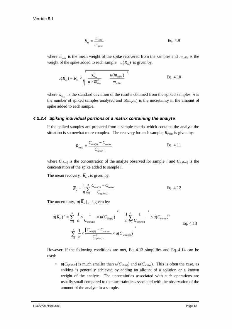
4.2.2.4 Spiking individual portions of a matrix containing the analyte

If the spiked samples are prepared from a sample matrix which contains the analyte thesituation is somewhat more complex. The recovery for each sample, Rm(i), is given by:

RC C

Cm iobs i native

spike i( )

( )

( )

=− Eq. 4.11

where Cobs(i) is the concentration of the analyte observed for sample i and Cspike(i) is theconcentration of the spike added to sample i.

The mean recovery, Rm , is given by:

Rn

C CCm

obs i native

spike ii

n

=−

=∑1

1

( )

( )

Eq. 4.12

The uncertainty, u Rm( ) , is given by:

( )

u Rn C

u Cn C

u C

n

C C

Cu C

mspike i

obs ispike ii

n

nativei

n

obs i native

spike ispike i

i

n

( ) ( ) ( )

( )

( )( )

( )

( )

( )( )

2

2

1

2

2

1

2

2

1

1 1 1 1

1

= × ×

+

×

+ ×−

×

==

=

∑∑

∑Eq. 4.13

However, if the following conditions are met, Eq. 4.13 simplifies and Eq. 4.14 can beused:

• u(Cspike(i)) is much smaller than u(Cobs(i)) and u(Cnative). This is often the case, asspiking is generally achieved by adding an aliquot of a solution or a knownweight of the analyte. The uncertainties associated with such operations areusually small compared to the uncertainties associated with the observation of theamount of the analyte in a sample.

Version 5.1


• The standard deviation of the Cspike(i) values is small compared to the mean of theCspike(i) values. If this condition is met, the mean of the Cspike(i) values, Cspike isused in the calculation. This is likely to be the case in recovery studies at asingle level using similar quantities of the sample matrix in the preparation ofeach spiked sample.

• The estimates of u(Cobs(i)) are all similar. In such cases the mean, u Cobs i( )( ) canbe used. Again, this is likely to be the case when each sample is spiked at thesame concentration so that all the Cobs(i) values are of a similar order ofmagnitude.

u RC

u Cn

u Cmspike

obs inative( )

( )( )( )= +1 2

2 Eq. 4.14

4.2.3 Estimating Rm and u( Rm ) by comparison with a standard method

Rm can be evaluated by analysing a typical sample using the method under evaluationand an alternative standard technique for which the uncertainty is known. It isrecommended that at least five determinations are made for each method. Rm is givenby:

RCCm

method

s dard

=tan

Eq. 4.15

where Cmethod is the mean of the results obtained using the method under considerationand Cs dardtan is the mean of the results obtained using the standard method. Theuncertainty in the recovery, u Rm( ) , is given by:

u R Rs

n Cu C

Cm mmethod

method

s dard

s dard

( )( )= ×

×

+

2

2

2

tan

tan

Eq. 4.16

where smethod is the standard deviation of the results obtained using the method, n is thenumber of replicates and u(Cstandard) is the standard uncertainty associated with thestandard method.

4.2.4 Other methods for estimating Rm and u( Rm )

If there are no CRMs or standard methods available, and spiking samples is impractical,alternative methods of investigating the recovery are required. However, such techniquesgenerally require an element of judgement on the part of the analyst and can only be usedas an initial indication of the uncertainty associated with method recovery. If the resultsof such a study indicate that the uncertainties associated with recovery are a significantcontribution to the uncertainty budget, further investigation will be required to obtain abetter estimate. Techniques include:

Version 5.1


4.2.4.1 Investigating extraction behaviour

One technique is the re-extraction of samples either under the same experimentalconditions, or preferably with a more vigorous extraction system (e.g., a strongerextraction solvent). The amount of analyte extracted under the normal method conditionsis compared with the total amount extracted (amount extracted initially plus the amountextracted by subsequent re-extractions). Rm is the ratio of these estimates. If re-extraction was achieved using the same conditions as the initial extraction, the differencebetween the true recovery and the assumed value of 1 is known to be at least 1- Rm . Thedifference could be greater, as repeated extractions under the same experimentalconditions may not quantitatively recover all of the analyte from the sample. It istherefore recommended that that uncertainty, u Rm( ) , associated with the assumed valueof Rm = 1 be estimated as (1- Rm ). If repeat extractions were carried out using a morevigorous extraction system, the confidence about the difference between Rm and theassumed value of 1 is greater, as it is more likely that repeat extractions will havequantitatively recovered the analyte. In such cases it is recommended that u Rm( ) isestimated as (1- Rm )/k, where k is the coverage factor that will be used to calculate theexpanded uncertainty.

In these cases it is already assumed that Rm is equal to 1 and the uncertainty has beenestimated accordingly. There is therefore no need to follow the procedures outlined inSection 4.2.5.

Another technique involves monitoring the extraction procedure with time and using theinformation to predict how much of the analyte present has been extracted. Thistechnique is described in detail elsewhere.[5, 7]

4.2.4.2 Analysis of a “worst case” CRM

If a CRM is available which has a matrix known to be more difficult to extract theanalyte from compared to test samples, the recovery observed for the CRM can provide aworst case estimate on which to base the recovery for real samples. If the matrix isknown to be extreme, compared to test samples, it is reasonable to assume that recoveriesfor test samples are more likely to be closer to 1 than to RCRM, the recovery for the CRM.It is therefore appropriate to take RCRM

as representing the lower limit of a triangulardistribution. As a first estimate, Rm is assumed to equal 1, with an uncertainty, u Rm( ) ,of:

u RR

mCRM( ) = −16

Eq. 4.17

Note that if there is no evidence to suggest where in the range 1-RCRM the recovery fortest samples is likely to lie, a rectangular distribution should be assumed. u Rm( ) istherefore given by 1- Rm /√3.

Since assumptions about Rm and u Rm( ) have been made at this stage, there is no need tofollow the procedures outlined in Section 4.2.5.

Version 5.1


These approaches to estimating Rm are discussed in more detail elsewhere.[5, 6]

4.2.5 Estimating the contribution of Rm to u(R)

Assuming an estimate of the recovery Rm and its uncertainty u Rm( ) has been obtainedusing one of the procedures outlined in Sections 4.2.1 to 4.2.4, three possible casesarise:[8, 9]

1. Rm , taking into account u Rm( ) , is not significantly different from 1 so results arenot corrected for recovery.

2. Rm , taking into account u Rm( ) , is significantly different from 1 and results arecorrected for recovery.

3. Rm , taking into account u Rm( ) , is significantly different from 1 but a correction isnot applied.

To determine whether the recovery is significantly different from 1 a significance test isused.[4] Calculate the test statistic t using the following equation:

tR

u Rm

m

=−1

( )Eq. 4.18

If the degrees of freedom associated with u Rm( ) are known, compare t with the 2-tailedcritical value, tcrit, for the appropriate number of degrees of freedom at 95% confidence.If t is less than the critical value then Rm is not significantly different from 1.

If the degrees of freedom associated with u Rm( ) are unknown, for example if there is acontribution from the uncertainty in the certified value of a reference material, compare twith k, the coverage factor that will be used in the calculation of the expandeduncertainty (see Section 5.2 for guidance on selecting an appropriate value for k).

If 1 − <R u R km m/ ( ) the recovery is not significantly different from 1.

If 1 − >R u R km m/ ( ) the recovery is significantly different from 1.

Case 1

The significance test indicates that the recovery is not significantly different from 1 sothere is no reason to correct analytical results for recovery. However, there is still anuncertainty associated with the estimate of Rm as the significance test could notdistinguish between a range of values about 1.0. If the test statistic was compared withtcrit the range is 1±tcrit u Rm( ) . The uncertainty associated with recovery in this case,u Rm( )' , is given by:

u Rt u R

mm( )'

( ).

crit= ×196

Eq. 4.19

Version 5.1


If the test statistic was compared with the coverage factor k, the range is1± ×k u Rm( ) .In this case the uncertainty associated with Rm is taken as u Rm( ) .

To convert to a relative standard deviation divide u Rm( ) or u Rm( )' by the assumed valueof Rm . In this case Rm = 1 so the standard deviation is equivalent to the relativestandard deviation.

Case 2

As a correction factor is being applied, Rm is explicitly included in the calculation of theresult. u Rm( ) is therefore included in the overall uncertainty calculation as the termu Rm( ) / Rm since the correction is multiplicative (see Section 5).

Case 3

In this case the recovery is statistically significantly different from 1, but in the normalapplication of the method no correction is applied (i.e., Rm is assumed to equal 1). Theuncertainty must be increased to take account of the fact that the recovery has not beencorrected for. The increased uncertainty, u Rm( )' ' , is given by:

u RR

ku Rm

mm( )' ' ( )= −

+12

2 Eq. 4.20

where k is the coverage factor which will be used in the calculation of the expandeduncertainty.

u Rm( )' ' is expressed as a relative standard deviation by dividing by the assumed value ofRm as in case 1.

4.2.6 Estimating Rs and u(Rs) from spiking studies

Where the method scope covers a range of sample matrices and/or analyte concentrationsan additional uncertainty term is required to take account of differences in the recovery ofa particular sample type, compared to the material used to estimate Rm . This is can beevaluated by analysing a representative range of spiked samples, covering typicalmatrices and analyte concentrations, in replicate. The number of matrices and levelsexamined, and the number of replicates for each sample will depend on the method scope.The same guidelines apply as for the precision studies discussed in Section 4.1.Calculate the mean recovery for each sample (see Eq. 4.12). Rs is assumed to be equal to1.0, however there will be an uncertainty in this assumption. This appears in the spreadof mean recoveries observed for the different spiked samples. The uncertainty, u(Rs), istherefore the standard deviation of the mean recoveries for each sample type.

Version 5.1


4.2.7 Estimating Rrep and u(Rrep)Rrep is generally assumed to equal one, indicating that the recovery from a spiked samplerepresents perfectly the recovery observed for incurred analyte. The uncertainty u(Rrep)is a measure of the uncertainty associated with that assumption, i.e., how different Rrep

might be from the assumed value of 1.

The complexity of evaluating how representative a spike is of the behaviour of nativematerial varies from matrix to matrix and with the method being studied. In some casesit can be argued that a spike is a good representation of a real sample, for example inliquid samples where the analyte is simply dissolved in the matrix. In addition, if themethod involves total dissolution or destruction of the matrix, for example by ashing,there may be no reason to believe that a spike would behave any differently from theincurred analyte. However, problems arise for more complex matrices and where themethod involves extraction rather than total destruction or dissolution. Possibleapproaches to investigating the performance of spiked versus real samples includemonitoring the extraction of spiked and native analytes with time, and comparison ofspiked recovery with the recovery from a less representative CRM. However, these maynot be appropriate in all cases. If experimental evidence on the appropriateness ofspiking cannot be obtained, then judgements and/or assumptions have to be made.Ideally, Rrep should be evaluated by the analysis of a reference material (even if it is notdirectly comparable to the test samples) and comparing the recovery obtained with thoseobserved from the spiking studies. The uncertainty u(Rrep) is then estimated as:

( )u RRk

u Rreprep

rep( ) ( )'=−

+

1 22 Eq. 4.21

where k is the coverage factor which will be used to calculate the expanded uncertaintyand u Rrep( ') is the uncertainty associated with the estimate of Rrep. The moststraightforward approach is to spike the CRM and compare the recovery observed withthat observed from the analysis of the unspiked reference material. In such cases Rrep isgiven by:

RC C

CC

Crepobs spike obs CRM

spike

CRM

obs CRM

=−

×( ) ( )

( )Eq. 4.22

where Cobs spike( ) is the mean concentration observed from replicate analyses of the spikedCRM, Cobs CRM( ) is the mean concentration observed from replicate analyses of theunspiked CRM, Cspike is the concentration of the spike added and CCRM is the certifiedconcentration of the reference material. The uncertainty, u Rrep( )' , obtained bydifferentiating Eq. 4.22:

( )u R Ru C

C Cu C u C

C C Cu C

Cu C

Crep repobs spike

obs spike obs CRM

obs CRM obs spike

obs CRM obs CRM obs spike

CRM

CRM

spike

spike

( )'( ) ( ) ( ) ( ) ( )( )

( ) ( )

( ) ( )

( ) ( ) ( )

= ×−

+

×× −

+

+

2 2 2 2

Eq. 4.23

Version 5.1


In this case, we are only interested in the dispersion of results obtained for the meanvalues Cobs spike( ) and Cobs CRM( ) . The corresponding uncertainties are therefore given bythe standard deviation of the mean of the observed concentrations in each case. Note thatthe above equation holds if the spiking study was based on the replicate analysis of asingled spiked sample of the CRM. If the study was based on the analysis of a numberof individual portions of the CRM (of similar weight) all spiked at a similarconcentration (see Section 4.2.2.4), Eq. 4.22 and Eq. 4.23 are modified slightly:

RC C

CC

Crepobs spike obs CRM

spike

CRM

obs CRM

=−

×( ) ( )

( )Eq. 4.24

( )u R Ru C

C Cu C u C

C C Cu C

Cu C

Crep repobs spike

obs spike obs CRM

obs CRM obs spike

obs CRM obs CRM obs spike

CRM

CRM

spike

spike

( )'( ) ( ) ( ) ( ) ( )( )

( ) ( )

( ) ( )

( ) ( ) ( )

= ×−

+

×× −

+

+

2 2 2 2

Eq. 4.25

where u Cobs spike( )( ) is the average of the uncertainties associated with each of theCobs(spike) values divided by the square root of the number of determinations of Cobs(spike),Cspike is the average of the concentrations of the spike added to each sample andu Cspike( ) is the average of the uncertainties associated with each of the Cspike values.

If there is no CRM available then judgements will have to made based on whateverinformation is available, for example, published studies. The estimation of Rrep isdiscussed in more detail elsewhere.[5, 6]

4.2.8 Calculating R and u(R)The recovery for a particular sample, R, is given by R R R Rm s rep= × × . However, sinceRs and Rrep are generally assumed to equal 1, R = Rm . The values of Rm andu Rm( ) used depend on whether or not Rm is significantly different from 1, and if so,whether a correction to the result for a particular sample is applied. This was discussedin Section 4.2.5. The uncertainty associated with R, u(R) is given by:

u R Ru R

Ru R

Ru R

Rm

m

s

s

rep

rep

( )( ) ( ) ( )

= ×

+

+

2 2 2

Eq. 4.26

However, if R Rs rep= = 1 , Eq. 4.26 simplifies to:

u R Ru R

Ru R u Rm

m

ms rep( )

( )( ) ( )= ×

+ +

22 2 Eq. 4.27

Version 5.1


4.3 Evaluation of other sources of uncertaintySources of uncertainty not adequately covered by the precision and trueness experimentsrequire separate evaluation. For example, a method may require that the sample isheated to a particular temperature. The method may specify a permitted range about thistemperature, e.g., heat to 100±5 °C. During the precision study the temperature may nothave been varied sufficiently to cover the full range of temperatures permitted in themethod specification. Alternatively there may be no method specification for a particularparameter. In both cases the effect of changes in the parameter on the result of theanalysis needs to be evaluated. Other sources of uncertainty which may requireevaluation include:

• purity of standards, e.g., if a single batch of material has been used to prepare allthe standards used during the precision study;

• calibration of glassware, e.g., if a single pipette was used throughout theprecision study;

• calibration e.g., if the same set of calibration standards was used throughout theprecision studies.

There are three main sources of data: calibration certificates and manufacturers’specifications; data published in the literature; specially designed experimental studies.Each of these is discussed below.

4.3.1 Calibration certificates and manufacturers’ specifications

For many sources of uncertainty, calibration certificates or suppliers’ catalogues providethe required information:

• Tolerances for volumetric glassware can be obtained from catalogues or theliterature supplied with the item.

• Data on the purity of standards and other reagents can be obtained from thesupplier.

• Calibration uncertainties for balances can be obtained from the calibrationcertificate.

Note that the information presented on calibration certificates, etc. may not be in theform of a standard uncertainty and must therefore be converted before combining withother uncertainty estimates. Details of how to do this are given in Annex 2.

4.3.2 Published data

As the aim of this guide is to give guidance on obtaining uncertainty estimates during themethod validation stage, it might be expected that very little published data would beavailable for a new procedure. This obviously depends on the method, but it may be that

Version 5.1


particular stages of the method have been investigated in the context of other methods sosome data may be available. For example, a sample pre-treatment step such a grindingor extraction may be common to a number of different methods; or the stability ofsamples or reagents used in a procedure may already have been investigated.

4.3.3 Experimental studies

If no existing data are available then the uncertainty must be investigated experimentally.As part of method development and validation, key method parameters are studied todetermine the effect of variations in them on the outcome of the analysis. If a significanteffect is observed for a particular parameter, appropriate control limits are set such thatvariations within the limits will not have a significant effect on the outcome of theanalysis. Alternatively, the method is improved by concentrating on the stages of themethod identified as critical. A common method of identifying the critical methodparameters is the ruggedness test. This involves making deliberate variations in themethod and investigating the effect on the result. An established technique forruggedness testing is described by the AOAC.[10] Such a test is also useful foruncertainty estimation. The results from ruggedness studies can be used in the evaluationof uncertainties associated with method parameters not adequately covered by theprecision and trueness studies. Such studies can also be used to identify significantsources of uncertainty which require further study. Suggested procedures for estimatinguncertainty via ruggedness testing are given in the following sections.

4.3.3.1 Designing a ruggedness test

The ruggedness testing procedure described by the AOAC[10] uses Plackett-Burmanexperimental designs.[11] Such designs allow the investigation of a number of methodparameters in a limited number of experiments. This section focuses on the experimentaldesign used for investigating seven experimental parameters.

Each of the seven parameters are investigated at two levels. Let A, B, C, D, E, F, Grepresent one set of values for the parameters under investigation. Let a, b, c, d, e, f, grepresent the alternative values for the parameters. If control limits have been set in themethod for a parameter (e.g., heat at 100±5 °C) the parameter should be investigated atthe extremes of the permitted range (i.e., 95 °C and 105 °C in the example given). If nocontrol limits have been specified it is up to the analyst to choose suitable values for theruggedness test. This can be based on knowledge gained from similar methods or duringthe development of the method being studied, or from knowledge of the normal variationof the parameter. For example, the method may require that the sample is left to stand atambient temperature. The analyst knows that the maximum variation in the laboratorytemperature is 20±5 °C. In the ruggedness test the sample would be left to stand at 15°C or 25 °C as required by the experimental design.

Variables such as temperature and time are known as continuous variables. Ruggednesstests can also be used to evaluate the effects of changes in non-continuous variables suchas the type of HPLC column used (e.g., C8 vs.C18).

Version 5.1


The ruggedness test should be carried out on a representative sample. If it is suspectedthat particular types of sample may behave in different ways, for example from datacollected in the recovery and precision studies or during the development of the method,they should be investigated separately and, if possible, the reasons for the differingresponse identified.

To investigate seven parameters, a minimum of 8 experiments are required using thefollowing experimental design:

Determination number

Parametervalue

1 2 3 4 5 6 7 8

A or a A A A A a a a a

B or b B B b b B B b b

C or c C c C c C c C c

D or d D D d d d d D D

E or e E e E e e E e E

F or f F f f F F f f F

G or g G g g G g G G g

Observedresult

s t u v w x y z

The effect of a particular parameter is estimated by subtracting the mean of the resultsobtained with the parameter at the alternative value from the mean of the results obtainedwith it at the initial value. For example, for parameter A the difference, DxA, iscalculated from:

DxA = ( ) ( )s t u v w x y z+ + +

−+ + +

4 4Eq. 4.28

Calculate the differences for all seven parameters and list them in order of magnitude.Note that the signs of the differences are unimportant. If variations in one or twoparameters are affecting the analysis then their differences will be substantially largerthan those for the other parameters. To determine whether variations in a parameter havea significant effect on the result, a significance test is used to determine if the differencecalculated above is significantly different from zero. The procedure is as follows:

1. Obtain an estimate of the within batch method precision, as a standard deviation, fromreplicate analysis of a representative sample over a short period of time.

2. Calculate the test statistic t:[12]

tn Dx

si=

××2

Eq. 4.29

Version 5.1


where s is the estimate of the method precision calculated in (1) above, n is the number ofexperiments carried out at each level for each parameter (n = 4 for the design givenabove), and Dxi is the difference calculated for parameter xi.

Compare t with the 2-tailed critical value, tcrit, for N-1 degrees of freedom at 95%confidence, where N is the number of determinations used in the estimation of s.

Case 1: If t is less than tcrit the difference is not significantly different from zero.Therefore, variations in the parameter do not have a significant effect on the methodperformance.

Case 2: If t is greater than tcrit the difference is significantly different from zero.Therefore, variations in the parameter have a significant effect on the methodperformance.

In both cases there is an uncertainty associated with the parameter. Procedures forestimating the uncertainties are given in the following sections.

4.3.3.2 Calculating uncertainties for case 1 parameters

Although the ruggedness study indicated that variations in the parameter do notsignificantly affect the method (i.e., the change in results on varying the parameter is notsignificantly different from zero), the significance test could not have distinguishedbetween values in the range 0±(√2 × tcrit × s)/√n). The uncertainty associated with thefinal result y due to parameter xi, is given by:

u y xt s

ni( ( )) crit real

test

= × ××

×2196.

δδ

Eq. 4.30

where δreal is the change in the parameter which would be expected when the method isoperating under control in routine use and δtest is the change in parameter that wasspecified in the ruggedness test. This term is required to take account of the fact that thechange in a parameter used in the ruggedness test may be much greater than thatobserved during normal operation of the method.

If the effect is proportional to the analyte concentration then the uncertainty should beconverted to a relative standard deviation by dividing by an estimate of the mean obtainedfrom replicate analysis of the sample used in the study under normal conditions, or if thisis not available, by the average of the eight results obtained in the ruggedness test. If,however, the effect is independent of analyte concentration the uncertainty should beexpressed as a standard deviation (see Section 5).

Version 5.1


4.3.3.3 Calculating uncertainties for case 2 parameters

To calculate the uncertainty for a particular parameter, xi, an estimate of the sensitivitycoefficient, ci, and the uncertainty in the parameter, u(xi), is required.

4.3.3.3.1 Estimating u(xi): For example, a method states that the sample must bedistilled for 120 minutes. The analyst estimates that the variation in thedistillation time in routine application of the method will be ±5 minutes. Theuncertainty in the distillation time is therefore 2.9 minutes (see Annex 2 forinformation on calculating standard uncertainties). Alternatively, controllimits can be set for the parameter to ensure that the resulting contribution tothe overall uncertainty is acceptable. If a parameter is already controlled byspecification (such as specifying a temperature as 4 ± 1°C), the specificationlimit represents the relevant uncertainty in the parameter, and should beconverted to a standard deviation.

4.3.3.3.2 Estimating ci: If the ruggedness test indicates that the parameter has asignificant effect on the result, the sensitivity coefficient can be estimatedfrom the results of the study:

c Observed change in resultChange in parameteri =

Eq. 4.31

If the parameter is found to be a significant source of uncertainty, or if abetter estimate of the effect of the parameter on the result is required, furtherexperimental study is needed. Evaluate the rate of change of the result withchanges in the parameter by carrying out a number of experiments with theparameter at a range of different values. Plot a graph of the result versus thevalue of the parameter. If the relationship is approximately linear, thesensitivity coefficient is equivalent to the gradient of the best fit line.

4.3.3.3.3 Calculate the uncertainty in the final result due to parameter xi, u(y(xi)),using:

u(y(xi)) = u(xi) × ci Eq. 4.32

If the effect is proportional to analyte concentration, convert the uncertainty toa relative standard deviation by dividing u(y(xi)) by y, where y is the resultobtained with the parameter at the value specified in the method.

Version 5.1


5. Calculation of combined standard andexpanded uncertainties

5.1 Combined standard uncertaintyFollowing the estimation of the individual components of the uncertainty using theprocedures outlined in Section 4, the next stage is to combine the standard uncertaintiesto give a combined standard uncertainty. How the individual uncertainty components arecombined depends on whether or not they are proportional to the analyte concentration.If the uncertainty component is proportional to the analyte concentration then it can betreated as a relative standard deviation. If, however, the uncertainty is fixed regardless ofthe analyte concentration then it should be treated as a standard deviation. This leads totwo possible cases:

5.1.1 All sources of uncertainty are proportional to the analyteconcentration

In this case all the individual uncertainty components should be converted to relativestandard deviations. For a result y which is affected by the parameters p, q, r ..... whicheach have uncertainties u(p), u(q), u(r) ..... the uncertainty in y, u(y) is given by:

u yy

u pp

u qq

u rr

( ) ( ) ( ) ( ).....=

+

+

+

2 2 2

Eq. 5.1

5.1.2 Some sources of uncertainty are independent of analyteconcentration

In such cases the uncertainty components that are independent of the analyteconcentration must be combined as standard deviations. The uncertainty in the result dueto parameters that are not concentration dependent, u(y)', is given by:

u(y)' = u p u q u r( ) ( ) ( ) .....2 2 2+ + + Eq. 5.2

To calculate the combined uncertainty in the result, u(y') at an analyte concentration y',the concentration dependent and concentration independent uncertainties are combined asfollows:

( ) ( )( ) ( )u y u y y

u yy

' ' '= + ×

2

2

Eq. 5.3

where u(y) is the combined concentration dependent uncertainties calculated usingEq. 5.1 and u(y)' is the combined concentration independent uncertainty calculated usingEq. 5.2.

Version 5.1


Note that when the uncertainty estimate is required for a single analyte concentration, theuncertainty components can be combined as either standard deviations or relativestandard deviations; it will make no difference to the final answer.

The flow chart in Figure 5 illustrates the different options for combining uncertainties.

no

multiple

concentrations

single

concentration

Does the method scope cover single or multiple analyte concentrations?

Are all uncertainty components

proportional to analyte concentration?

Are the uncertainty components quoted as standard deviations or

relative standard deviations?

Combine uncertainties using equation 5.1



relative standard yes

standard

Figure 5: Flow chart illustrating the options for combining uncertainty components

deviations deviations

START

END

5.2 Expanded uncertaintyThe combined standard uncertainty obtained in Section 5.1 must be multiplied by anappropriate coverage factor, k, to give the expanded uncertainty. The expandeduncertainty is an interval which is expected to include a large fraction of the distributionof values reasonably attributable to the measurand. For a combined standard uncertaintyu(y), the expanded uncertainty U(y) is given by:

U(y) = k × u(y) Eq. 5.4

The choice of coverage factor depends on knowledge of the use to which the result is put,the degree of confidence required and knowledge of the degrees of freedom associatedwith individual uncertainty components. For most purposes a coverage factor of k = 2 isrecommended (however, see note below). For a normal distribution a coverage factor of2 gives an interval containing approximately 95% of the distribution of values.

For a higher level of confidence, k is chosen as 3. For a normal distribution a coveragefactor of 3 gives an interval containing over 99.6% of the distribution of values.

Note: The use of coverage factors of 2 and 3 to give levels of confidence ofapproximately 95% and 99.6% respectively assumes that there are a reasonable

Version 5.1


number of degrees of freedom associated with the estimates of the majorcontributions to the uncertainty budget. In this guide it is recommended that atleast 10 determinations are carried out in the precision and trueness studies. If it isnot possible to obtain this many replicates and either of these factors dominate theuncertainty budget, the coverage factor should be obtained from the table ofcritical values for the Student t test. For example, if the dominant contribution tothe uncertainty budget was based on only 4 determinations this would give 3degrees of freedom. The 2-tailed tcrit value at the 95% confidence level is 3.182. Itcan therefore be seen that using uncertainty estimates based on only a smallnumber of determinations will have a significant effect on the coverage factor andhence on the expanded uncertainty.

Version 5.1


6. Reporting uncertainty

6.1 Reporting expanded uncertaintyThe Eurachem Guide[2] gives the following guidance:

Unless otherwise required, the result y should be stated together with the expandeduncertainty, U(y), calculated using a coverage factor of k = 2 (or other appropriatecoverage factor, see Section 5.2). The following form is recommended:

“(result): y ± U(y) (units)

[where] the reported uncertainty is [an expanded uncertainty as defined in theInternational Vocabulary of Basic and General terms in Metrology, 2nd, ed., ISO, 1993]calculated using a coverage factor of 2, [which gives a level of confidence ofapproximately 95%.]”

Terms in [ ] may be omitted or abbreviated as appropriate.

6.2 Reporting standard uncertaintyThe Eurachem Guide[2] gives the following guidance:

When uncertainty is expressed as the combined standard uncertainty u(y) the followingform is recommended:

“(result): y (units) [with a] standard uncertainty of u(y) (units) [where standarduncertainty is defined in the International Vocabulary of Basic and General terms inMetrology, 2nd, ed., ISO, 1993 and corresponds to one standard deviation.]”

The use of the symbol ± is not recommended when using standard uncertainty.

6.3 DocumentationA simple proforma for summarising uncertainty budgets is given in Annex 5. This canbe used to summarise details of the sources of uncertainty included in the budget, howthey were estimated and their magnitudes. There is also a section for the combinedstandard and expanded uncertainty.

Version 5.1


Annex 1: Cause and Effect Analysis

As discussed in Section 3, uncertainty estimation requires the production of a structured list ofpossible sources of uncertainty. One way of producing such a list is cause and effectanalysis.[13] The principles of the construction of cause and effect diagrams are described fullyelsewhere,[13] and detailed discussions of their application to uncertainty estimation, withexamples, have been published.[14, 15] The use of cause and effect diagrams has three mainstages: construction, refinement and experimental design (also called reconciliation). An outlineof the process is presented below.

A1.1 Construction of a cause and effect diagram

A cause and effect diagram consists of a hierarchical structure of “causes” which culminate in asingle outcome or “effect”. A typical diagram for an analytical method is given in Figure A1.1.In terms of uncertainty estimation, the “effect” is the result obtained from the analysis. Themain branches feeding into it represent the parameters used in the calculation of the result.Combining the uncertainties associated with these parameters will give the uncertainty in thefinal result. The stages in the construction are:

A1.1.1 Write the complete equation used to calculate the result, including any intermediatecalculations. The parameters in the equation form the main branches of the diagram. It isalmost always necessary to add a main branch representing overall bias, usually as recovery.

A1.1.2 Consider each branch in turn and add additional branches representing effects which willcontribute to the uncertainties in the parameters identified in A1.1.1. For example, theuncertainty in the weight of sample taken for analysis will have contributions from the balanceprecision and calibration. Branches representing these terms should therefore feed into the mainbranch representing the sample weight.

A1.1.3 For each branch added in A1.1.2, add further branches representing any additional contributoryfactors. Continue the process until the effects become sufficiently remote.

A1.2 Refinement of the cause and effect diagram

Refinement of the diagram involves the resolution of duplicate terms and rearrangement of thebranches to clarify contributions and group related causes. This process results in a simplifiedcause and effect diagram which can be used as a checklist to ensure that all sources ofuncertainty have been considered in the uncertainty budget. Duplications of terms in thediagram are resolved using the rules given in Section 3.4.

Figure A1.2 shows a typical cause and effect diagram after refinement.

A1.3 Experimental design

The final stage in the process is the planning of experiments which will provide the informationrequired to obtain an estimate of the combined uncertainty for the method. Initially, two sets ofexperiments are carried out - a precision study and a trueness study. These experiments are

Version 5.1


planned in such a way that as many of the sources of uncertainty identified in the cause andeffect diagram as possible are covered. The diagram is used as a checklist, and thoseparameters not adequately covered by the precision and trueness experiments are evaluatedseparately. Section 4 discusses the types of experiments required and gives details of how thedata obtained are used to calculate uncertainty.

Key to Figure A1.1 and Figure A1.2

Equation used to calculate the concentration of all-trans retinol, C all trans− in µg 100 g-1, in asample of infant formula:

CA V C

A Wall transS F STD

STD S− = × ×

×

where:

AS is the peak area recorded for the sample solution;

ASTD is the peak area recorded for the standard solution;

VF is the final volume of the sample solution (ml);

WS is the weight of sample taken for analysis (g);

CSTD is the concentration of the standard solution (µg ml-1).

In the cause and effect diagrams:

C flask/pipette calibration;

T temperature effects;

BC balance calibration;

L balance linearity.

Version 5.1


Annex 2: Calculating standarduncertainties

When estimating uncertainty, a variety of existing information may be available, e.g.,calibration certificates. This information may not be expressed in the form of a standarddeviation and must therefore be converted before it can be combined with other standarduncertainties. Some common cases are given below.

1. The uncertainty is expressed as a confidence interval with a given level of confidence.For example, a certificate states that the concentration of an analyte in a certifiedreference material is 100±0.5 mg kg-1 with 95% confidence.

To convert to a standard uncertainty, divide by the appropriate percentage point of theNormal distribution for the level of confidence given. For 95% confidence divide by1.96.

2. The uncertainty is expressed as an expanded uncertainty calculated using a givencoverage factor. For example, documentation supplied with a solution states that itsconcentration is 1000±3 mg l-1 where the reported uncertainty is an expandeduncertainty calculated using a coverage factor k = 2 which gives a level of confidenceof approximately 95%.

To convert to a standard uncertainty, divide by the stated coverage factor.

3. Limits of ±x are given without a confidence level or coverage factor. For example,the manufacturer’s specification for the stated volume of a 100 ml volumetric flask isquoted as ±0.08 ml. It is normally appropriate to assume a rectangular distributionwith a standard deviation of x/√3.

To convert to a standard uncertainty, divide by √3.

Version 5.1


Annex 3: Definitions

Bias

The difference between the expectation of the test results and an accepted referencevalue.[16]

Note: Bias is the total systematic error as contrasted to random error. There may be one ormore systematic error components contributing to the bias. A larger systematicdifference from the accepted reference value is reflected by a larger bias value.

Coverage factor

The numerical factor, k, used as a multiplier of the combined standard uncertainty inorder to obtain an expanded uncertainty.[1]

Note: A coverage factor is typically in the range 2 to 3. A coverage factor of 2 gives a level ofconfidence of approximately 95%.

Critical value

The critical value (e.g. tcrit in a t-test) is the tabulated value of the test statistic obtained ina significance test. The critical value is obtained from statistical tables by reading thevalue given for the appropriate number of degrees of freedom and the desired level ofconfidence.[4] In this guide, two-tailed tcrit values at the 95% confidence level are alwaysused.

Degrees of freedom

The term n-1 in the expression for the sample standard deviation, s, is called the numberof degrees of freedom (abbreviated to dof or ν in statistical tables). In general it is thenumber of data points, n, less the number of parameters already estimated from the data.In the expression for the sample standard deviation the number of degrees of freedom isn-1 as the mean has already been estimated from the data. Knowledge of the number ofdegrees of freedom is needed for obtaining the appropriate critical value from statisticaltables for significance tests. In general it is equivalent to n-1.

Expanded uncertainty

Quantity defining an interval about the result of a measurement that may be expected toencompass a large fraction of the distribution of values that could reasonably beattributed to the measurand.[1] The expanded uncertainty, U(y), is calculated from thecombined standard uncertainty u(y) and a coverage factor k using:

U(y) = k × u(y)

Version 5.1


F-test

The F-test is a significance test used to compare two variances, s12 and s2

2 , where s isthe standard deviation. Calculate the test statistic:

F = ss

12

22

where s12 is the larger of the two variances (this will guarantee that F≥1). Compare F

with the appropriate critical value, Fcrit, at n1-1 and n2-1 degrees of freedom. If F is lessthan Fcrit there is no significant difference between the variances. For a 2-tailed test at the95% confidence level, the appropriate critical value is obtained from statistical tables forthe 97.5% confidence level.[4]

Measurement uncertainty

Parameter associated with the result of a measurement, that characterises the dispersionof values that could reasonably be attributed to the measurand.[17]

Note: The parameter may be, for example, a standard deviation (or given multiple of it), or thewidth of a confidence interval. Uncertainty of measurement comprises, in general, manycomponents. Some of these components may be evaluated from the distribution of theresults of a series of measurements and can be characterised by experimental standarddeviations. The other components, which can also be characterised by standarddeviations, are evaluated from assumed probability distributions based on experience orother information. It is understood that the result of the measurement is the bestestimate of the value of the measurand and that all components of uncertainty, includingthose arising from systematic effects, contribute to the dispersion.

Precision

The closeness of agreement between independent test results obtained under stipulatedconditions.[16]

Note: Precision depends only on the distribution of random errors and does not relate to thetrue value or specified value. The measure of precision is usually expressed in terms ofimprecision and calculated as a standard deviation of the test results.

Recovery

The ratio of the observed value to the expected value.

Note: The expected value can be either the certified value of a reference material or theconcentration of a fortified or spiked sample. In analytical chemistry, recovery is oftenused as a measure of the trueness of a method.

Version 5.1


Relative standard deviation

The relative standard deviation, RSD, of a set of results with standard deviation s andmean x is given by:

RSDsx

=

Sample standard deviation

The standard deviation of n results with a mean x is given by:

sx x

n

ii

n

=−

−=∑ ( )2

1

1

Sensitivity coefficient

The sensitivity coefficient describes how the observed output varies with changes in theinput parameter. For example, for a result y and a parameter xi, the sensitivitycoefficient ci describing the effect of changes in xi on y is given by:

c Observed change in yChange in xi

i

=

Significance test

A statistical test used to decide whether there are significant differences between theproperties of different sets of data at a given level of confidence. A test statistic iscalculated and compared with a tabulated critical value. If the test statistic is greaterthan the critical value this indicates a significant difference between the properties beingcompared. Examples of significance tests include the t-test which can be used tocompare the mean of a set of results with a stated value, or to compare the means of twoindependent sets of results; and the F-test which is used to compare the variances of twosets of data.[4]

Version 5.1


Standard deviation of the mean

The standard deviation of the mean, sx , of n samples with standard deviation s is givenby:

s snx =

Standard uncertainty

Uncertainty of the result of a measurement expressed as a standard deviation.[1] For aresult xi, the standard uncertainty is u(xi).

Trueness

The closeness of agreement between the average value obtained from a large set of testresults and an accepted reference value.[16]

Note: The measure of trueness is normally expressed in terms of bias.

Uncertainty budget

List of parameters and their associated uncertainties which contribute to the uncertaintyfor the method as a whole. The individual uncertainties in the uncertainty budget arecombined to give the standard and expanded uncertainties for the method.

Version 5.1


Annex 4: Worked examples

A4.1 The determination of vitamin A and vitamin E in infant formula

A4.1.1 Outline of method

The method was developed for the determination of tocopherol, retinol and caroteneisomers in a range of food stuffs. This example considers the validation and calculationof an uncertainty estimate specifically for the determination of all-trans retinol (vitaminA) and α-tocopherol (vitamin E) in infant formula. The homogenised sample ishydrolysed to release the retinol and tocopherol isomers. These are then extracted intomixed ethers and the extract concentrated. Portions of the extract are chromatographedon different HPLC systems to separate and quantify the isomers required. A normalphase system is used for the determination of α-tocopherol whilst a reversed phasesystem is used for the determination of all-trans retinol. In each case calibration is bymeans of a single standard prepared by serial dilution of a stock solution. Theconcentration of the analyte in a sample, Cvit, is given by:

CvitS F STD

STD S

A V CA W

= × ××

where:


ASTDis the peak area recorded for the standard solution;


WS is the weight of sample taken for analysis (g);

CSTD is the concentration of the standard solution (µg ml-1).

A flow diagram illustrating the stages in the method is presented in Figure A4.1 andcause and effect diagrams are given in Annex 1.


Weigh sample

Saponify for 30 minsunder reflux

Add 1 g pyrogallol and150 ml ethanolic KOH soln

Transfer solution to a separating funnel

Add 500 ml mixed ethers

Extract vitamins into mixedethers

Wash ether extract with water until washsolutions are neutral to phenolphthalein

Transfer washed ether extract to amberrotary evaporation flask

Add 2 ml BHT soln

Evaporate to dryness at 40°C

Dissolve in appropriatevolume of methanol*

Quantify all-trans retinol onreverse phase HPLC system

Remove appropriate volume of solution by pipette*

Add 2 ml BHT soln

Evaporate to dryness on rotary evaporator

Dissolve in appropriatevolume of mobile phase*

Quantify α-tocopherol onnormal phase HPLC system

Butylated hydroxy toluene

* The final volume of eachsolution for HPLC shouldbe selected such that theconcentration of eachvitamin present is close tothat of the relevantcalibration standard

Figure A4.1: Flow diagram illustrating stages in the method for the determination of all-trans retinoland tocopherols in infant formula

Version 5.1


A4.1.2 Precision study

A survey of the nutritional labelling of commercially available infant formula indicatedthat that they were all of broadly comparable composition (fat, protein and carbohydratelevels) and contained similar concentrations of vitamin A and vitamin E. Three sampleswere chosen to cover the widest possible range of vitamin concentrations. Each samplewas analysed a total of four times, in four separate extraction and HPLC runs. For eachHPLC run fresh calibration standards and mobile phase were prepared. In addition, acertified reference material (SRM 1846) was analysed in replicate for the estimation ofRm (see below). These results were included in the precision study. The results aresummarised in Table A4.1.§

Table A4.1: Summary of results from precision studies on the determination of all-trans retinol andα-tocopherol

all-trans retinol α-tocopherol

Sample mean(mg kg-1)

standarddeviation(mg kg-1)

relativestandarddeviation

n mean(mg kg-1)

standarddeviation(mg kg-1)


n

Infant formula A 9.67 0.146 0.0151 4 64.08 2.411 0.0376 4

Infant formula B 10.40 0.247 0.0238 4 69.05 2.156 0.0312 4

Infant formula C 6.67 0.217 0.0325 4 171.93 7.959 0.0463 4

SRM 1846 5.32 0.285 0.0536 6 278.51 10.663 0.0383 6

The standard deviations observed for all-trans retinol were of a similar order ofmagnitude. This indicates that within the range of analyte concentrations studied, thestandard deviation is independent of analyte concentration. In this case, the uncertaintyassociated with method precision, u(P), for samples with all-trans retinol concentrationsranging from approximately 5 mg kg-1 to 10 mg kg-1, was estimated as the pooledstandard deviation. This was obtained using Eq. 4.1:

( ) ( ) ( ) ( )spool =

× + × + × + ×+ +

=

3 0146 3 0 247 3 0 217 5 0 285

3 3 3 50 238

2 2 2 2. .

+

. ..

u(P) for all-trans retinol is therefore 0.238 mg kg-1.

§ Note: The examples given in Annex 4 were calculated using a spreadsheet. The values presented inthe tables and equations have been rounded. Reproducing the calculations with the values given maytherefore result in slightly differing answers.

Version 5.1


For α-tocopherol, the relative standard deviations observed for the different samples wereall of a similar order of magnitude. This indicates that the standard deviation isapproximately proportional to analyte concentration, across the range studied. In suchcases it is appropriate to pool the relative standard deviations to obtain the estimate ofu(P), using Eq. 4.2:

( ) ( ) ( ) ( )RSDpool =

× + × + × + ×+ + +

=

3 0 0376 3 0 0312 3 0 0463 5 0 0383

3 3 3 50 0387

2 2 2 2. . ..

.

u(P)/P for α-tocopherol is therefore 0.0387 as a relative standard deviation.

A4.1.3 Trueness study

Calculation of Rm and u( Rm )

In this case a certified reference material, SRM 1846 produced by the National Instituteof Standards and Technology (NIST), was available. The CRM is an infant formulacertified for a number of vitamins, including all-trans retinol and α-tocopherol. Sixportions of the CRM were analysed. The results, together with the certified values forthe material, are summarised in Table A4.2.

Table A4.2: Results from the analysis of infant formula SRM 1846

Certified values Observed values

Analyte ConcentrationCCRM

(mg kg-1)

Quoteduncertainty(mg kg-1)1

Standarduncertainty

u(CCRM)(mg kg-1)2

MeanCobs

(mg kg-1)

standarddeviation

sobs(mg kg-1)

all-trans retinol 5.84 0.68 0.35 5.32 0.285

α-tocopherol 271 25 12.8 278.51 10.6631 The quoted uncertainty is an expanded uncertainty given at the 95% confidence level.2 The standard uncertainty is obtained by dividing the expanded uncertainty by 1.96.

Eq. 4.3 and Eq. 4.4 were used to calculate Rm and u Rm( ) respectively.

For all-trans retinol:

Rm = =532 584 0 911. / . .

Version 5.1


u Rm( ) = ××

+

=0 911

0 2856 5 32

0 35584

0 05812

2

2

..

...

.

Similar calculations for α-tocopherol gave values of Rm = 1.028 and u Rm( ) = 0.0511.

To determine the contribution of Rm to the combined uncertainty, the value calculatedabove was compared with 1, using Eq. 4.18. For all-trans retinol:

t = − =1 0 9110 0581

153.

..

In this case, t was compared with the coverage factor, k = 2. As t is less than two thereis no evidence to suggest that Rm is significantly different from 1. Rm was thereforeassumed to equal 1 with an uncertainty, u Rm( ) , of 0.0581 (see Section 4.2.5, case 1). Asimilar calculation for α-tocopherol also indicated that Rm was not significantly differentfrom 1. u Rm( ) was therefore estimated as 0.0511.

Calculation of u(Rs)

Rs was estimated from spiking studies on infant formula A used in the precision study. Itwas not possible to produce a homogeneous bulk spiked sample so individual portions ofthe infant formula were spiked at the required concentration. Samples were prepared atthe concentrations indicated in Table A4.3. Four samples were analysed at eachconcentration, in separate extraction and HPLC batches. The samples were spiked byadding solutions of all-trans retinol and α-tocopherol to approximately 10 g of sample ina saponification flask, prior to the addition of any other reagents. The mean recovery foreach sample was calculated using Eq. 4.12. Cnative was taken as the mean of the resultsobtained from the precision study. The results are summarised in Table A4.3.

Table A4.3: Summary of results from the study of Rs for the determination of all-trans retinoland α-tocopherol

all-trans retinol α-tocopherol

Spiking level Approxtarget

concentration(mg kg-1)

Meanrecovery

n Approxtarget

concentration(mg kg-1)

Meanrecovery

n

1 14.0 0.981 4 84.0 1.028 4

2 18.0 0.991 4 99.0 1.103 4

3 22.0 0.996 4 114.0 1.167 4

u(Rs ) 0.00767 u(Rs ) 0.0696

Version 5.1


u(Rs) is the standard deviation of the mean recoveries obtained at each concentration.

Calculation of R and u(R)

In this case, as a representative CRM was available for the estimation of Rm and u Rm( )for both all-trans retinol and α-tocopherol, there was no need for the Rrep term. Both Rm

and Rs are assumed to be equal to 1. R is therefore also equal to 1. u(R) was calculatedusing Eq. 4.26. For all-trans retinol:

u R( ) = + =0 0581 0 00767 0 05862 2. . .

A similar calculation for α-tocopherol gives an estimate of u(R) = 0.0863. Note thatsince in both cases R = 1, the uncertainty is the same whether expressed as a standarddeviation or a relative standard deviation.

A4.1.4 Evaluation of other sources of uncertainty

Ruggedness study

There were a number of method parameters which were not representatively variedduring the precision and trueness studies. These were investigated using a ruggednessstudy. The extraction and HPLC stages of the method were examined in separatestudies. Only the ruggedness study for all-trans retinol is presented. A similar studywould be required for α-tocopherol to complete the uncertainty budget. The parametersinvestigated and the levels chosen are summarised in Table A4.4 and Table A4.5 below.The study was carried out on the Certified Reference Material.

Table A4.4: Parameters investigated in the ruggedness study of the extractionprocedure for all-trans retinol

Parameter Value

Weight KOH used in ethanolic KOH A 42 g a 21 g

Saponification time B 20 mins b 40 mins

Number of 250 ml ether extractions C 2 c 1

Shaking time for each ether extraction D 2 mins d 1 min

Number of water washes* E to neutral e 3 extra

Rotary evaporation time** F to dryness f 5 additionalmins

Rotary evaporation temperature G 30 °C g 50 °C

* The method currently states that the ether extract should be washed with water until thewash extracts are neutral. For parameter (e) the ether extract was washed with a further3 portions of water.

** The method currently states that the sample extract should be evaporated to dryness.

Version 5.1


For parameter (f) the evaporation was continued for a further 5 minutes after drynesshad been reached.

Table A4.5: Parameters investigated in the ruggedness study of the HPLC procedurefor the determination of all-trans retinol

Parameter Value

Column age A' new a' old

Flow rate B' 0.8 ml min-1 b' 1.2 ml min-1

Dummy variable C' + c' -

Mobile phase composition(methanol/water)

D' 90/10 d' 95/5

Injection volume E' 15 µl e' 25 µl

Detection wavelength F' 320 nm f' 330 nm

Column temperature G' 30 °C g' oven off

Results

The results from the ruggedness studies were evaluated as described in Section 4.3.3.

Extraction and clean-up stage

The results obtained from the ruggedness testing of the extraction procedure for all-transretinol are presented in Table A4.6. The differences for each parameter, DxA to DxG,were calculated as described in Section 4.3.3.1.

Table A4.6: Results form the ruggedness testing of the extraction of all-transretinol from infant formula

Observed result (mg kg-1)

s t u v w x y z

5.25 3.98 4.22 4.43 5.51 4.78 4.35 4.96

Calculated differences

DxA DxB DxC DxD DxE DxF DxG

-0.4329 0.3898 0.2948 -0.1009 0.2387 0.7036 0.03608

The precision for the method had previously been estimated as 0.238 mg kg-1 with 14degrees of freedom (see Section A4.1.2). Using Eq. 4.29, t values were calculated for

Version 5.1


each parameter. These were then compared with the critical value tcrit = 2.145 (2-tailed,ν = 14, 95% confidence). The results are presented below:

Table A4.7: Identification of parameters having a significant effect onthe extraction of all-trans retinol from infant formula

Parameter t value Significanteffect at 95%confidence?

Weight KOH used in ethanolic KOH 2.573 Yes

Saponification time 2.316 Yes

Number of 250 ml ether extractions 1.752 No

Shaking time for each ether extraction 0.599 No

Number of water washes 1.419 No

Rotary evaporation time 4.181 Yes

Rotary evaporation temperature 0.214 No

In cases where the effect of a parameter was found not to be significant, Eq. 4.30 wasused to calculate the uncertainty:

u y xireal

test

real

test

( ( )) = × ××

× = ×2 2145 0 2384 196

0184. .

..

δδ

δδ

Number of ether extractions

The method specifies two ether extractions. In the ruggedness study, the effect of usingonly one ether extraction was investigated. The results indicated that using only oneextraction reduced the recovery of all-trans retinol, although the effect was notsignificant. If the method is applied correctly it is unlikely that δreal would equal δtest.However, there is likely to be some variation in the efficiency of the extractions fromanalysis to analysis, due to variations in the vigour with which the mixture is shaken.This effect will be covered by the estimate of uncertainty associated with precision. Forthese reasons, an additional uncertainty has not been included for this parameter.

Shaking time for ether extractions

The method was developed using a shaking time of 2 minutes per extraction. In theruggedness test this was reduced to 1 minute. δtest is therefore equal to 1 minute. It isestimated that during normal operation of the method, the shaking time might varybetween 1.5 minutes and 2.5 minutes. δreal is therefore also 1 minute. u(y(xD)) istherefore 0.184 mg kg-1.

Version 5.1


Number of water washes

The method currently specifies that the ether extract should be washed with 150 mlportions of water until the wash solution is neutral to phenolphthalein. The results of theruggedness test indicate that additional washes of the extract beyond this leads to lowerresults. In the ruggedness study the effect of three extra washes was investigated(δtest = 3). During routine use of the method it was considered unlikely that as many asthree extra washes would be carried out. However, one additional wash may be likely,particularly if neutrality has only just been reached on the previous wash. δreal wastherefore estimated as being equal to 1. The uncertainty, u(y(xE)), is therefore 0.0613.

Rotary evaporation temperature

The method has been developed using a rotary evaporation temperature of 40°C. It isestimated that this is controlled to ±2°C in normal use (i.e., δreal = 4°C). In theruggedness test the temperature was set at 30°C and 50°C, giving a δtest value of 20°C.u(y(xG)) is therefore 0.0368 mg kg-1.

For parameters identified as having a significant effect on the extraction, the proceduredescribed in Section 4.3.3.3 was followed.

Weight of potassium hydroxide used to prepare ethanolic potassium hydroxidesolution

Under normal operating conditions, 42±0.1 g potassium hydroxide is used in thepreparation of the ethanolic potassium hydroxide solution required for the saponificationreaction. In the ruggedness study the amount of potassium hydroxide used was reducedby 21 g. This resulted in a difference, DxA, of -0.4329 mg kg-1. Using Eq. 4.31, thesensitivity coefficient, cA, was calculated as:

cA = =0 432921

0 0206.

. mg kg-1 g-1

The uncertainty in the parameter, u(xA), was obtained from the control limit on the weightof potassium hydroxide specified in the method, assuming a rectangular distribution.Therefore, u(xA) = 0.1/√3 = 0.0577 g. The uncertainty in the final result due tovariations in parameter A, u(y(xA)) was calculated using Eq. 4.32:

u y xA( ( )) = × =0 0577 0 0206 0 00119. . . mg kg-1

Saponification time

The method was developed using a saponification time of 30 minutes. It is estimated thatduring routine use of the method this will vary by ±5 minutes, giving an uncertainty, uB,of 2.89 minutes (assuming a rectangular distribution). In the ruggedness study theparameter was varied from 20 minutes to 40 minutes. This resulted in a difference, DxB,of 0.3898 mg kg-1. The sensitivity coefficient, cB, is therefore 0.0195 mg kg-1 min-1. Theuncertainty in the final result due to variation in this parameter, u(y(xB)), is therefore0.0564 mg kg-1.

Version 5.1


Rotary evaporation time

The results of the ruggedness study showed that allowing the rotary evaporation tocontinue after the sample had reached dryness caused a reduction in the amount ofall-trans retinol observed. This is likely to be due to decomposition of the analyte. In theruggedness study, rotary evaporation was allowed to continue for an extra 5 minutesafter dryness had been reached. This resulted in a difference, DxF, of 0.7036 mg kg-1.The sensitivity coefficient is therefore 0.141 mg kg-1 min-1. In the routine application ofthe method, it was estimated that the rotary evaporation may continue for between 0 and5 minutes after dryness has been reached. This was taken as a rectangular distribution of2.5±2.5 minutes. uF is therefore equal to 1.443 minutes. The uncertainty, u(y(xF)), istherefore 0.203 mg kg-1.

The effect of all the above parameters was considered to be proportional to the analyteconcentration. The uncertainties were therefore converted to relative standard deviationsby dividing by 5.32 mg kg-1, the mean of the results obtained from previous analyses ofSRM 1846 under normal method conditions.

HPLC stage

The results from the ruggedness testing of the HPLC procedure for the determination ofall-trans retinol are presented in Table A4.8.

Table A4.8: Results form the ruggedness testing of the HPLC procedure for the determinationof all-trans retinol

Observed result (mg kg-1)

s t u v w x y z

5.47 5.33 5.35 5.07 4.59 4.75 4.79 5.09


DxA' DxB' DxC' DxD' DxE' DxF' DxG'

0.4997 -0.04021 -0.01202 0.2291 0.2192 -0.000975 -0.06682

The calculated differences were tested for significant variation from zero. The standarddeviation used in the significance test was based on pooled within batch precision datafrom three standard solutions of all-trans retinol, each analysed four times. This gave apooled standard deviation of 0.167 mg kg-1 (ν = 9). The appropriate tcrit value, at the95% confidence level, is 2.262.

For parameters identified as having no significant effect, the uncertainty was estimated as0.136 × (δreal/δtest) using Eq. 4.30.

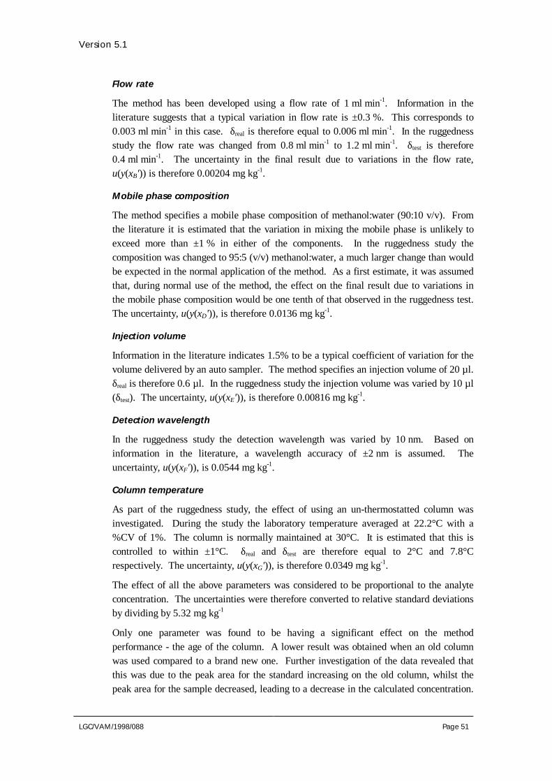
Version 5.1


Flow rate

The method has been developed using a flow rate of 1 ml min-1. Information in theliterature suggests that a typical variation in flow rate is ±0.3 %. This corresponds to0.003 ml min-1 in this case. δreal is therefore equal to 0.006 ml min-1. In the ruggednessstudy the flow rate was changed from 0.8 ml min-1 to 1.2 ml min-1. δtest is therefore0.4 ml min-1. The uncertainty in the final result due to variations in the flow rate,u(y(xB')) is therefore 0.00204 mg kg-1.

Mobile phase composition

The method specifies a mobile phase composition of methanol:water (90:10 v/v). Fromthe literature it is estimated that the variation in mixing the mobile phase is unlikely toexceed more than ±1 % in either of the components. In the ruggedness study thecomposition was changed to 95:5 (v/v) methanol:water, a much larger change than wouldbe expected in the normal application of the method. As a first estimate, it was assumedthat, during normal use of the method, the effect on the final result due to variations inthe mobile phase composition would be one tenth of that observed in the ruggedness test.The uncertainty, u(y(xD')), is therefore 0.0136 mg kg-1.

Injection volume

Information in the literature indicates 1.5% to be a typical coefficient of variation for thevolume delivered by an auto sampler. The method specifies an injection volume of 20 µl.δreal is therefore 0.6 µl. In the ruggedness study the injection volume was varied by 10 µl(δtest). The uncertainty, u(y(xE')), is therefore 0.00816 mg kg-1.

Detection wavelength

In the ruggedness study the detection wavelength was varied by 10 nm. Based oninformation in the literature, a wavelength accuracy of ±2 nm is assumed. Theuncertainty, u(y(xF')), is 0.0544 mg kg-1.

Column temperature

As part of the ruggedness study, the effect of using an un-thermostatted column wasinvestigated. During the study the laboratory temperature averaged at 22.2°C with a%CV of 1%. The column is normally maintained at 30°C. It is estimated that this iscontrolled to within ±1°C. δreal and δtest are therefore equal to 2°C and 7.8°Crespectively. The uncertainty, u(y(xG')), is therefore 0.0349 mg kg-1.

The effect of all the above parameters was considered to be proportional to the analyteconcentration. The uncertainties were therefore converted to relative standard deviationsby dividing by 5.32 mg kg-1

Only one parameter was found to be having a significant effect on the methodperformance - the age of the column. A lower result was obtained when an old columnwas used compared to a brand new one. Further investigation of the data revealed thatthis was due to the peak area for the standard increasing on the old column, whilst thepeak area for the sample decreased, leading to a decrease in the calculated concentration.

Version 5.1


The results of the ruggedness test indicate that as the column ages the methodperformance will change. During routine application of the method this should bemonitored using an HPLC QC standard. Only when this is performing adequately (afteradjustment of the HPLC conditions if necessary) will sample extracts be presented foranalysis. Due to the relatively short timescale it is unlikely that the precision studyundertaken as part of the validation study would include variability in methodperformance due to column ageing. However, when the method is in routine use a checksample will be analysed and data collected over a period of time. The variation observedin these results will include the variability due to changes in the column performance,within the bounds permitted by the HPLC QC standard. If the long term precisionestimate obtained from the QC sample is significantly different from that obtained fromthe precision study described earlier, then it can be used to generate a revised uncertaintyestimate at a later data. For the above reasons, an estimate of the uncertainty due toageing of the HPLC column has not been included in the present uncertainty budget.

Remaining sources of uncertainty

The precision and trueness studies were designed to cover as many of the sources ofuncertainty as possible (see cause and effect diagram, Figures A1.1 and A1.2), forexample, by analysing a range of concentration levels, and by preparing new standardsand HPLC mobile phase for each batch of analyses. Parameters which were notadequately varied during these experiments, such as the extraction and HPLC conditions,were investigated in the ruggedness tests. There are however, a small number ofparameters which were not covered by the above experiments. These generally related tothe calibration of volumetric glassware and balances used in the preparation of thestandards and samples. For example, during this study the same balance was used toweigh out all the samples. Although the precision associated with this operation isincluded in the overall precision estimate, the effect of the accuracy of the balance hasnot been included in the uncertainty budget so far. The balance used in the study maytypically have a positive bias of 0.0001 g. In the future a different balance, or the samebalance after re-calibration, may have a negative bias of 0.0001 g. Since this possiblevariation is not already included in the uncertainty budget it should be consideredseparately. However, previous experience[18] has shown us that uncertainties associatedwith the calibration of analytical balances and volumetric glassware are generally smallcompared to other sources of uncertainty such as overall precision and recovery.Additional uncertainty estimates for these parameters have not therefore been included inthe uncertainty budget.

Version 5.1


A4.1.5 Calculation of combined and expanded uncertainties

Table A4.9 presents the magnitudes of the individual uncertainty components for thedetermination of all-trans retinol in infant formula.

Table A4.9: Uncertainty budget for the determination of all-trans retinolin infant formula

Parameter Standard uncertainty

Precision u(P) 0.238 mg kg-1

Recovery u(R) 0.0586

Weight KOH used in ethanolic KOH u(y(xA)) 0.000224

Saponification time u(y(xB)) 0.0106

Shaking time for each ether extraction u(y(xD)) 0.0346

Number of water washes u(y(xE)) 0.0115

Rotary evaporation time u(y(xF)) 0.0382

Rotary evaporation temperature u(y(xG)) 0.00692

Flow rate u(y(xB')) 0.000383

Mobile phase composition u(y(xD')) 0.00256

Injection volume u(y(xE')) 0.00153

Detection wavelength u(y(xF')) 0.0103

Column temperature u(y(xG')) 0.00656

Note that standard uncertainties given without units are expressed as relativestandard deviations.

The sources of uncertainty that were identified as being proportional to analyteconcentration were combined by calculating the root sum of squares as in Eq. 5.1:

u yy( ) = 0 0809.

This was combined with the uncertainty associated with method precision, which wasfound to be independent of analyte concentration, using Eq. 5.3. For example, for asample containing 5 mg kg-1 all-trans retinol:

( )u y( )' . . .= + × =0 238 5 0 0809 0 472 2 mg kg-1

Similar calculations lead to the following estimates of uncertainty for a range of typicalall-trans retinol concentrations:

Version 5.1


Table A4.10: Standard uncertainty estimates for the determination ofall-trans retinol in infant formula

Concentration(mg kg-1)

Standard uncertainty(mg kg-1)

Relative standarduncertainty

5 0.47 0.094

7.5 0.65 0.087

10 0.84 0.084

Expanded uncertainties were obtained by multiplying the standard uncertainties by acoverage factor, k = 2, which gives a level of confidence of approximately 95%:

Table A4.11: Expanded uncertainty estimates for the determinationof all-trans retinol in infant formula

Concentration(mg kg-1)

Expandeduncertainty

(mg kg-1)

Relative expandeduncertainty

5 0.94 0.19

7.5 1.30 0.17

10 1.69 0.17

Comments on uncertainty budget

Figure A4.2 illustrates the contributions to the measurement uncertainty for thedetermination of all-trans retinol in infant formula at a concentration of 5 mg kg-1. Thevertical line indicates one third of the magnitude of the largest contribution to theuncertainty budget (in this case recovery). Only parameters with uncertainties greaterthan this value need to be considered as significant sources of uncertainty for the method.In this case the four major contributions were identified as precision and recovery for theentire method, and the effects of the length of time each ether extract is shaken with waterand of evaporating the ether extract to dryness. Both the latter uncertainties wereevaluated using data from the ruggedness test. The test is designed to highlight theparameters which have a significant effect on method performance and also to give aninitial uncertainty estimate for each parameter. If the uncertainty estimate so obtained isa significant contribution to the uncertainty estimate, ideally the effects of changes in thatparameter should be investigated further. In this case, for example, that could involveseparate studies to investigate the effect of shaking time and rotary evaporationconditions on the result of the analysis. It will then be possible to include a refineduncertainty estimate in the uncertainty budget. If the uncertainties associated with these

Version 5.1


parameters are unacceptably large, the parameters will have to be more strictly controlledin the method protocol, for example by specifying a shaking time of 2 minutes±10seconds. If it is not possible to control the parameter sufficiently, i.e., if the controllimits required would be so tight as to be impossible to achieve during routine applicationof the method, then further method development will be required.

0 0.005 0.01 0.015 0.02 0.025 0.03 0.035 0.04 0.045 0.05 0.055 0.06

Uncertainty as a relative standard deviation

Precision

Recovery

Weight KOH

Saponification time

Shaking time

No. water washes

Rotary evaporation time

Rotary evaporation temp

Flow rate

Mobile phase composition

Injection volume

Detection wavelength

Column temp

Par

amet

er

Figure A4.2: Contributions to the measuremrnt uncertainty for the determination of all-trans retinol in infant formula

(analyte concentration 5 mg kg-1)

1/3rd largest uncertainty component

Version 5.1


A4.2 The determination of markers in oils

A4.2.1 Outline of method

The quantification of three markers - solvent red 24, quinizarin and solvent yellow 124 -in oils is required. The samples are analysed by reversed phase high performance liquidchromatography with UV-visible diode array detection, after a clean up stage. Thesample (10 ml) is passed through a 500 mg silica cartridge. The cartridge is washedunder vacuum with 10 ml hexane to remove residual oil. The solvent red 24, quinizarinand solvent yellow 124 are then eluted under gravity with 10 ml butan-1-ol in hexane(butan-1-ol 10% v/v). The eluant is evaporated to dryness under a stream of air, heatingif necessary, and the residue dissolved in 2.5 ml acetonitrile. The solution is placed in anultrasonic bath for 5 minutes and then filtered through a 0.45µm filter. 50 µl of theresulting solution is analysed by HPLC using a 5 µm phenyl-hexyl column(250 mm x 4.6 mm) with a gradient elution of water and acetonitrile at a flow rate of1 ml min-1. The column is maintained at a temperature of 30 °C. Detection is by meansof a diode array detector set at 475 nm for the determination of solvent yellow 124 and500 nm for the determination of solvent red 24 and quinizarin. Calibration is by meansof a single standard in acetonitrile containing solvent red 24 and solvent yellow 124 at aconcentration of 20 mg l-1, and quinizarin at a concentration of 10 mg l-1. Theconcentration of the markers, Cmarker in mg l-1, is given by:

CA V C

A VS F STD

STD Smarker = × ×

×

where:


ASTDis the peak area recorded for the standard solution;


VS is the volume of the sample taken for analysis (ml);

CSTD is the concentration of the standard solution (mg l-1).

A flow diagram illustrating the main stages in the method is presented in Figure A4.3.

Version 5.1


Transfer 10 ml sample by pipette onto a500 mg silica SPE cartridge

Drain under vacuum until cartridge is dry

Wash cartridge under vacuumwith 10 ml hexane

Elute markers from cartridge under gravitywith 10 ml butan-1-ol in hexane (10% v/v)

Evaporate eluant to dryness under airstream, heating if necessary

Dissolve residue in 2.5 ml acetonitrile

Filter solution through0.45µm filter

Quantify markers using reverse phaseHPLC with diode array detection

Figure A4.3: Flow diagram illustrating the stages in the method for thedetermination of markers in diesel oil

Version 5.1


A4.2.2 Precision study

Samples of three types of unmarked oils (A to C) were fortified with solvent red 24,quinizarin and solvent yellow 124 according to Table A4.12, giving a total of 15samples.

Table A4.12: Samples prepared for precision study on the determination of markers inoil

Concentration of compound in sample (mg l-1)Analyte Sample 1 Sample 2 Sample 3 Sample 4 Sample 5

Solvent red 24 0.041 1.02 2.03 3.05 4.06

Quinizarin 0.040 0.498 0.996 1.49 1.99

Solvent yellow 124 0.040 1.20 2.40 3.99 4.99

Oil B was a diesel sample, and this represented a sample of typical viscosity. Oil A wasa kerosene and oil C was a lubricating oil. These oils are respectively less viscous andmore viscous than oil B. Initially, 12 sub-samples of the diesel (B) sample 3 wereanalysed. The extraction of the samples was carried out in two batches of six onconsecutive days. The markers in all 12 samples were quantified in a single HPLC runwith the order of analysis randomised. The results are summarised in Table A4.13 (notethat analysis of one of the samples for quinizarin was unsuccessful, giving n = 11). Thisinitial study was followed by the analysis, in duplicate, of all 15 samples. The results aresummarised in Table A4.14, Table A4.15 and Table A4.16.

Table A4.13: Summary of results from the replicate analysis of matrixB fortified at concentrations of 2.03 mg l-1 solvent red 24, 0.996 mg l-1

quinizarin and 2.40 mg l-1 solvent yellow

Analyte mean(mg l-1)

standarddeviation

(mg l-1)


n

Solvent red 24 1.92 0.0621 0.0323 12

Quinizarin 0.913 0.0216 0.0236 11

Solvent yellow 124 2.35 0.0251 0.0107 12

Version 5.1


Table A4.14: Summary of results from the duplicate analysis of oil samples spikedwith solvent red 24 at a range of concentrations

Matrix Target conc(mg l-1)

Observed conc(mg l-1)

mean Difference Normaliseddifference

A 0.041 0.033 0.036 0.035 -0.003 -0.0883

A 1.02 0.989 0.969 0.979 0.019 0.0199

A 2.03 1.96 1.98 1.97 -0.016 -0.00837

A 3.05 2.98 2.88 2.93 0.098 0.0334

A 4.06 3.99 4.01 4.00 -0.019 -0.00474

B 0.041 0.044 0.036 0.040 0.007 0.181

B 1.02 0.945 0.927 0.936 0.018 0.0191

B 2.03 1.98 1.96 1.97 0.013 0.00669

B 3.05 2.83 2.90 2.87 -0.065 -0.0226

B 4.06 3.90 3.88 3.89 0.025 0.00650

C 0.041 0.039 0.040 0.040 -0.001 -0.0195

C 1.02 0.921 0.963 0.942 -0.043 -0.0455

C 2.03 1.93 1.87 1.90 0.064 0.0339

C 3.05 2.96 3.02 2.99 -0.061 -0.0205

C 4.03 3.92 4.04 3.98 -0.120 -0.0302

s 0.0532 0.0585

s/√2 0.0376 0.0414

Version 5.1


Table A4.15: Summary of results from the duplicate analysis of oil samples spikedwith quinizarin at a range of concentrations



mean Differences Normaliseddifference

A 0.040 0.030 0.029 0.030 0.001 0.0398

A 0.498 0.359 0.360 0.360 -0.002 -0.00422

A 0.996 0.743 0.700 0.722 0.042 0.0587

A 1.49 0.999 1.13 1.07 -0.135 -0.127

A 1.99 1.58 1.59 1.58 -0.013 -0.00815

B 0.040 0.030 0.027 0.029 0.003 0.100

B 0.498 0.421 0.443 0.432 -0.023 -0.0529

B 0.996 0.909 0.892 0.900 0.018 0.0196

B 1.49 1.37 1.35 1.36 0.022 0.0160

B 1.99 1.88 1.87 1.88 0.010 0.00533

C 0.040 0.034 0.031 0.032 0.003 0.0954

C 0.498 0.355 0.248 0.302 0.107 0.354

C 0.996 0.779 0.665 0.722 0.114 0.158

C 1.49 1.20 1.11 1.16 0.089 0.0769

C 1.99 1.53 1.63 1.58 -0.095 -0.0602

s 0.0664 0.111

s/√2 0.0470 0.0788

Version 5.1


Table A4.16: Summary of results from the duplicate analysis of oil samples spikedwith solvent yellow 124 at a range of concentrations



mean Differences Normaliseddifference

A 0.040 0.038 0.031 0.034 0.007 0.206

A 1.20 1.16 1.15 1.16 0.009 0.00796

A 2.40 2.32 2.27 2.30 0.054 0.0236

A 3.99 3.78 3.80 3.79 -0.022 -0.00574

A 4.99 4.86 4.82 4.84 0.041 0.00857

B 0.040 0.032 0.036 0.034 -0.004 -0.121

B 1.20 1.16 1.14 1.15 0.020 0.0173

B 2.40 2.37 2.32 2.35 0.052 0.0220

B 3.99 3.90 3.85 3.88 0.054 0.0139

B 4.99 4.97 4.93 4.95 0.039 0.00781

C 0.040 0.043 0.040 0.041 0.003 0.0780

C 1.20 1.17 1.15 1.16 0.024 0.0211

C 2.40 2.38 2.30 2.34 0.081 0.0348

C 3.99 3.85 3.81 3.83 0.041 0.0107

C 4.99 4.79 4.85 4.82 -0.057 -0.0118

s 0.0349 0.0656

s/√2 0.0247 0.0464

In addition, a sample of diesel spiked with the three markers was analysed 48 times in 3batches of 16 analyses as part of the trueness study (see Section A4.2.3). The results aresummarised in Table A4.17. The estimates of stotal were obtained from analysis ofvariance (ANOVA).[4]

Solvent Red 24

In the case of solvent red 24, there was no statistically significant difference between thethree estimates of the relative standard deviation obtained (see Table A4.13, Table A4.14and Table A4.17), although the test was borderline. This indicates that across the rangestudied (0.04 mg l-1 to 4 mg l-1) the precision is approximately proportional to analyteconcentration. However, to avoid producing an uncertainty estimate which would be anunder estimate for any particular matrix or concentration, it was decided to use theestimate of 0.0414 as a “worst case” uncertainty associated with precision, u(P). Thisestimate was obtained from the analysis of different matrices and concentrations and istherefore likely to be a more representative of the precision across the method scope.

Version 5.1


Quinizarin

The various estimates of the standard deviation and relative standard deviation were notcomparable. In particular, the estimates obtained from the duplicate results weresignificantly different from the other estimates. However, there were no obvious patternsin the data so no particular matrix and/or concentration could be identified as being thecause of the variability. There was therefore no justification for removing any data andrestricting the coverage of the uncertainty estimate, as in the case of solvent yellow 124(see below). The results of the precision studies indicate that the method is more variableacross different matrices and analyte concentrations for quinizarin than for the othermarkers. The uncertainty associated with the precision was therefore taken as theestimate of the relative standard deviation obtained from the duplicate results, 0.0788.This represents a worst case estimate but it should ensure that the uncertainty is notunderestimated for any given matrix or concentration (although it may result in anoverestimate in some cases).

Solvent yellow 124

There was no significant difference between the estimates of the relative standarddeviation obtained for samples at concentrations of 2.4 mg l-1 and 4.99 mg l-1. However,the estimate obtained from the duplicate analyses was significantly greater than the otherestimates. Inspection of that data revealed that the normalised differences observed forthe samples at a concentration of 0.04 mg l-1 were substantially larger than thoseobserved at the other concentrations. Removing these data points gave a revised estimateof the relative standard deviation of 0.00903. This was in agreement with the otherestimates obtained (F-tests, 95% confidence). The three estimates were therefore pooledusing Eq. 4.2 to give a single estimate of the relative standard deviation of 0.0114. As itstands, the uncertainty estimate cannot be applied to samples with concentrations below1.2 mg l-1. Further study would be required to investigate in more detail the precision atthese low levels.

A4.2.3 Trueness study

Calculation of Rm and u( Rm )

In this case there was no suitable CRM available for the evaluation of Rm . The bestoption available was to use spiked samples. In this example, the behaviour of spikedsamples is likely to be a good representation of that of test samples, as oils are markedsimply by adding and mixing in the required amount of the markers. A 2000 ml sampleof unmarked BP diesel was spiked with standards in toluene containing solvent red 24,quinizarin and solvent yellow 124 at concentrations of 0.996 mg ml-1, 1.02 mg ml-1 and1.97 mg ml-1 respectively to give concentrations in the diesel of 4.06 mg l-1, 1.99 mg l-1

and 4.99 mg l-1 respectively. Forty-eight aliquots of this sample were analysed in threebatches of 16 analyses. The results are summarised in Table A4.17.

Version 5.1


Table A4.17: Results from the replicate analysis of a diesel oil spiked with solvent red 24,quinizarin and solvent yellow 124

Analyte Targetconcentration

Cspike(mg l-1)

MeanCobs

(mg l-1)

Standarddeviation ofthe mean,

smean(mg l-1)a

Totalstandard

deviation,stotal (mg l-1)b

Relativestandarddeviation

Solvent red 24 4.06 3.88 0.0360 0.112 0.0289

Quinizarin 1.99 1.89 0.00370 0.0256 0.0136

Solvent yellow 124 4.99 4.99 0.0167 0.0618 0.0124aEstimated from ANOVA of 3 groups of 16 replicates according to ISO 5725:1994[19]

bEstimated from ANOVA[4]

Rm was calculated as described in Section 4.2.2.1. The mean recovery and itsuncertainty were calculated using Eq. 4.5 and Eq. 4.6 respectively, where smean given inTable A4.17 is equivalent to sobs/√n.

For solvent red 24:

Rm = =388 4 06 0 956. / . .

Based on information on the purity of the material used to prepare the spiked sample, andthe accuracy and precision of volumetric glassware and analytical balances used, theuncertainty in the concentration of solvent red 24 in the sample, u(Cspike), was estimatedas 0.05 mg l-1.** The uncertainty in Rm is therefore given by:

u Rm( ) = ×

+

=0 956

0 0360388

0 054 06

0 01482 2

...

.

..

The uncertainties associated with the concentration of quinizarin and solvent yellow 124in the spiked sample were estimated as 0.025 mg l-1 and 0.062 mg l-1 respectively.Similar calculations as above for quinizarin and solvent yellow 124 produced thefollowing estimates:

quinizarin: Rm = 0.949, u Rm( ) = 0.0121

solvent yellow 124, Rm = 1.00, u Rm( ) = 0.0129

To determine the contribution of Rm to the combined uncertainty, the value calculatedabove was compared with 1, using Eq. 4.18. For solvent red 24:

** Detailed information on the estimation of uncertainties of this type is presented in reference 2

Version 5.1


t = − =1 0 9560 0148

2 97.

..

In this case, t was compared with coverage factor, k = 2. A t value greater than twosuggests that Rm is significantly different from 1. However, in the normal application ofthe method, no correction will be made to take account of the fact that the methodrecovery is significantly different from 1. This is an example of case 3 discussed inSection 4.2.5. Accordingly, Eq. 4.20 was used to calculate the uncertainty u Rm( )' ' :

u Rm( )' ' = −

+ =1 0 956

20 0148 0 0262

22.

. .

The significance test also indicated that the recovery of quinizarin was significantlydifferent from 1. Applying Eq. 4.20 gives a value of u Rm( )' ' of 0.0283. In the case ofsolvent yellow 124, the significance test indicated that Rm was not significantly differentfrom 1. This is an example of case 1 discussed in Section 4.2.5. In such cases theuncertainty associated with Rm is the value of u Rm( ) calculated above (i.e., 0.0129).

Calculation of Rs

Rs was calculated using the results from the samples analysed in the precision study andthe data from the determination of Rm . u(Rs) is the standard deviation of the meanrecoveries obtained for the different matrices and analyte concentrations. The data aresummarised in Table A4.18 to Table A4.20.

Version 5.1


Table A4.18: Summary of recovery data for solvent red 24

Matrix Target concentration(mg l-1)

Mean recovery n

diesel oil 4.06 0.957 48

A 0.041 0.857 2

A 1.02 0.964 2

A 2.03 0.971 2

A 3.05 0.962 2

A 4.06 0.985 2

B 0.041 0.986 2

B 1.02 0.922 2

B 2.03 0.970 2

B 2.03 0.947 12

B 3.05 0.941 2

B 4.06 0.958 2

C 0.041 0.975 2

C 1.02 0.928 2

C 2.03 0.935 2

C 3.05 0.983 2

C 4.06 0.986 2

standard deviation (s) 0.0322

Version 5.1


Table A4.19: Summary of recovery data for quinizarin


Mean recovery n

diesel oil 1.99 0.949 48

A 0.040 0.745 2

A 0.498 0.722 2

A 0.996 0.725 2

A 1.49 0.714 2

A 1.99 0.794 2

B 0.040 0.725 2

B 0.498 0.868 2

B 0.996 0.904 2

B 0.996 0.945 11

B 1.49 0.910 2

B 1.99 0.941 2

C 0.040 0.806 2

C 0.498 0.606 2

C 0.996 0.725 2

C 1.49 0.775 2

C 1.99 0.792 2


Version 5.1


Table A4.20: Summary of recovery data forsolvent yellow 124


Mean recovery n

diesel oil 4.99 1.00 48

A 0.040 0.857 2

A 1.20 0.966 2

A 2.40 0.959 2

A 3.99 0.949 2

A 4.99 0.970 2

B 0.040 0.841 2

B 1.20 0.957 2

B 2.40 0.979 2

B 2.40 0.978 12

B 3.99 0.971 2

B 4.99 0.992 2

C 0.040 1.04 2

C 1.20 0.969 2

C 2.40 0.977 2

C 3.99 0.958 2

C 4.99 0.966 2


s excluding recoveries at 0.04 mg l-1 0.0138

For solvent red 24, the standard deviation of the mean recoveries obtained at variousconcentrations and from various matrices was calculated as 0.0322. As discussed inSection 4.2.6, this was used as the estimate of u(Rs).

In the case of quinizarin, the standard deviation of the mean recoveries was 0.0932. Thelarge standard deviation is due to the fact that the recoveries obtained for matrix B weregenerally higher than those obtained for matrices A or C. In this example, a singleuncertainty estimate will be reported for all the matrices studied. However, if thisestimate was found to be unsatisfactory for future applications of the method, separatebudgets could be calculated for individual matrices.

Version 5.1


Due to the problems associated with the precision of the determination of solventyellow 124 at low concentrations discussed in Section A4.2.2, the present uncertaintybudget will not cover samples with a concentration below 1.2 mg l-1. When calculatingu(Rs) the results obtained for samples containing 0.04 mg l-1 were therefore discounted.This resulted in a standard deviation of mean recoveries of 0.0138. This was taken asthe estimate of u(Rs).

Calculation of R and u(R)

As mentioned previously, in this example a spiked sample can be considered a reasonablerepresentation of test samples of marked diesel oils, as fuel is marked simply by addingthe required quantity of the marker. There is therefore no need for Rrep and u(Rrep) terms.Both Rm and Rs are assumed to be equal to 1. R is therefore also equal to 1. u(R) iscalculated using Eq. 4.26. For solvent red 24:

u R( ) = + =0 0262 0 0322 0 04152 2. . .

Similar calculations for quinizarin and solvent yellow 124 give values of 0.0974 and0.0187 respectively.

A4.2.4 Evaluation of other sources of uncertainty

Ruggedness study

There were a number of method parameters which were not adequately varied during theprecision and recovery studies. These were investigated using a ruggedness test asdescribed in Section 4.3.3. The extraction and HPLC stages of the method wereexamined separately. The parameters studied and the levels chosen are presented inTable A4.21 and Table A4.22. The ruggedness test was applied to matrix B sample 3used in the precision study (see Table A4.12).

Table A4.21: Parameters investigated in the ruggedness study of the extractionprocedure for the determination of markers in oil

Parameter Value

Brand of silica cartridges A Brand A a Brand B

Sample volume B 10 ml b 12 ml

Rate of elution of oil with hexane C vacuum c gravity

Volume of hexane wash D 12 ml d 8 ml

Conc butan-1-ol/hexane E 12% e 8%

Vol 10% butan-1-ol/hexane F 12 ml f 8 ml

Evaporation temperature G 50 °C g 80 °C

Version 5.1


Table A4.22: Parameters investigated in the ruggedness study of the HPLCprocedure for the determination of markers in oil

Parameter Value

Grade of acetonitrile in mobile phase A' Far UV a' HPLC

Flow rate B' 0.8 ml min-1 b' 1.2 ml min-1

Injection volume C' 40 µl c' 60 µl

Column temperature D' 25 °C d' 35 °C

Detector wavelength (A) E' 465 nm e' 485 nm

Mobile phase degassing F' degassed f' not degassed

Detector wavelength (B) G' 490 nm g' 510 nm

Results

The results from the ruggedness studies were evaluated as described in Section 4.3.3.

Extraction stage

The results obtained from the ruggedness testing of the extraction procedure for solventred 24, quinizarin and solvent yellow 124 are presented in Table A4.23. The differencesfor each parameter, DxA to DxG were calculated as described in Section 4.3.3.1.

Version 5.1


Table A4.23: Results form the ruggedness testing of the extraction of solvent red 24,quinizarin and solvent yellow 124 from fuel

Solvent red 24

Observed result (mg l-1)

s t u v w x y z

2.02 2.00 2.12 2.17 1.87 1.71 2.34 2.36



0.0075 -0.3525 0.0275 0.2125 -0.0425 0.0625 -0.0275

Quinizarin


s t u v w x y z

1.10 1.06 1.15 1.01 0.96 0.86 1.28 1.26



-0.0075 -0.18 0.07 0.1775 0.0175 -0.005 -0.0425

Solvent yellow 124 (mg l-1)

Observed result

s t u v w x y z

2.41 2.38 2.52 2.66 2.19 2.15 2.76 2.87



-0.0025 -0.4225 -0.02 0.225 -0.01 0.08 0.0075

The precision of the method for the analysis of the sample used in the ruggedness studyhad previously been estimated as:

solvent red 24: 0.0621 mg l-1 (ν = 11)

quinizarin: 0.0216 mg l-1 (ν = 10)

solvent yellow 124: 0.0251 mg l-1 (ν = 11)

Using Eq. 4.29, t values were calculated for each parameter and each analyte. Thesewere compared with the appropriate critical values of t at 95% confidence (tcrit = 2.201for solvent red 24 and solvent yellow 124, and 2.228 for quinizarin).

Version 5.1


Solvent red 24

In cases were the effect of a parameter was found not to be significant, Eq. 4.30 wasused to calculate the uncertainty:

u y xireal

test

real

test

( ( )) = × ××

× = ×2 2 201 0 06214 196

0 0493. .

..

δδ

δδ

Brand of silica cartridge

The ruggedness test investigated the effect of changing between brands of silica cartridge.Since this is likely to happen during the routine application of the method, δreal can beconsidered as being equal to δtest. The uncertainty, u(y(xA)), is therefore 0.0493 mg l-1.

Rate of elution of oil with hexane

The effect of the rate of elution of oil by hexane from the cartridge was investigated bycomparing the difference between elution under a vacuum and elution under gravity.When the method is used routinely, the oil will be eluted under vacuum. Variations in thevacuum applied from one extraction to another will affect the rate of elution of the oiland the amount of oil eluted. However, the effect of variations in the vacuum will besmall compared to the effect of having no vacuum present. It can therefore be assumedthat variations in the observed concentration of the markers, due to variability in thevacuum, will be small compared to the differences observed in the ruggedness test. As afirst estimate, the effect of variation in the vacuum during routine application of themethod was estimated as one tenth of that observed during the ruggedness study.

Concentration of butan-1-ol in hexane

The method was developed using a concentration of 10% (v/v) butan-1-ol in hexane.Based on the manufacturers’ specification and typical precision data for the volumetricglassware used to prepare the solution, it was estimated that the concentration may varyby ±0.1% (v/v), i.e., δreal is 0.2% (v/v). From the ruggedness test, δtest is equal to4% (v/v). The uncertainty, u(y(xE)), is therefore 0.00247 mg l-1.

Volume of 10% (v/v) butan-1-ol in hexane

The method was developed using 10 ml of 10% (v/v) butan-1-ol in hexane for elution ofthe markers. The likely variation in this volume was estimated as ±0.04 ml (based on themanufacturer’s specification for the pipette and typical precision data for pipettes of thistype). In the ruggedness test, the volume was changed by 4 ml. δreal and δtest are thereforeequal to 0.08 ml and 4 ml respectively. The uncertainty, u(y(xF)), is therefore0.000986 mg l-1.

Version 5.1


Evaporation temperature

The method currently specifies that samples are evaporated to dryness at 50°C. Theuncertainty in this value during routine use of the method was estimated as ±5°C. δreal istherefore 10°C. δtest was 30°C. The uncertainty u(y(xG)) is therefore 0.0164 mg l-1.

For parameters identified as having a significant effect on the extraction, the proceduredescribed in Section 4.3.3.3 was followed.

Sample volume

In the routine application of the method, 10 ml of sample is taken for analysis using anautomatic pipette. The uncertainty associated with this volume was estimated as0.04 ml. In the ruggedness test, the volume was increased to 12 ml. This resulted in adifference, DB, of -0.3525 mg l-1. The sensitivity coefficient, cB, is therefore0.1763 mg l-1 ml-1. The uncertainty, u(y(xB)), was therefore calculated as 0.00705 mg l-1.

Volume of hexane wash

The method was developed using 10 ml hexane (added by pipette) to wash the silicacartridge. The uncertainty associated with the volume delivered was estimated as0.04 ml. This is u(xD). Eq. 4.31 was used to calculate the sensitivity coefficient, cD:

cD = =0 21254

0 05313.

. mg l-1 ml-1

The uncertainty in the final result due to variation in parameter D, u(y(xD)) wascalculated using Eq. 4.32:

u y xD( ( )) . . .= × =0 04 0 05313 0 00213 mg l -1

The effect of all these parameters was considered to be proportional to the analyteconcentration. The uncertainty was therefore converted to a relative standard deviationby dividing by, 1.92 mg l-1, the mean of the results obtained from previous analyses ofthe sample under normal method conditions.

Quinizarin

For the parameters identified as not having a significant effect on the methodperformance, u(y(xi)) was calculated as 0.0174 × (δreal/δtest) using Eq. 4.30. Theuncertainties were converted to relative standard deviations by dividing by 0.909 mg l-1.


Using the same arguments applied in the case of solvent red 24, the uncertainty wascalculated as 0.0174 mg l-1.


Version 5.1


Again applying the same reasoning as in the case of solvent red 24, the uncertainty wasestimated as 0.000868 mg l-1.


The uncertainty was calculated as 0.000347 mg l-1, as discussed previously.

For the parameters identified as being significant, the following uncertainty estimateswere calculated:

Sample volume

The uncertainty was calculated as 0.00360 mg l-1, using the same reasoning as applied tosolvent red 24.


As discussed above, the effect on the final result of variations in the vacuum when elutingthe oil from the cartridge with hexane was estimated as one tenth that observed in theruggedness test. The uncertainty, u(y(xC)) was therefore estimated as 0.0070 mg l-1.


The uncertainty was evaluated as described in the case of solvent red 24. This resulted inan uncertainty of 0.00177 mg l-1.


The uncertainty in the evaporation temperature was based on the assumption that thetemperature could be controlled to ±5 °C. This was taken as a rectangular distributionand converted to a standard uncertainty by dividing by √3. The uncertainty u(y(xG)) istherefore 0.00409 mg l-1.

Solvent yellow 124

For the parameters identified as not having a significant effect on the methodperformance, u(y(xi)) was calculated as 0.0199 × (δreal/δtest) using Eq. 4.30. Theuncertainties were converted to relative standard deviations by dividing by 2.35 mg l-1.


Using the same arguments applied in the case of solvent red 24, the uncertainty wascalculated as 0.0199 mg l-1.


This was treated as for solvent red 24, giving an uncertainty of 0.00199 mg l-1.


Again applying the same reasoning as in the case of solvent red 24, the uncertainty wasestimated as 0.0010 mg l-1.

Version 5.1



The uncertainty was calculated as 0.00663 mg l-1, following the reasoning given forsolvent red 24.

For the parameters identified as being significant, the following uncertainty estimateswere calculated:

Sample volume

The uncertainty was calculated as 0.00845 mg l-1, using the same reasoning as applied tosolvent red 24.


As for the other two markers, the volume of the hexane wash clearly influences therecovery of solvent yellow 124. Using the procedure described for solvent red 24, theuncertainty u(y(xD)) was calculated as 0.00225 mg l-1.


The results indicate that the volume of butan-1-ol/hexane used to elute the marker has asignificant effect on recovery. As in the case of the hexane wash, the solution was addedby automatic pipette. The uncertainty u(y(xF)) was therefore calculated in the same way.u(y(xF)) is therefore equal to 0.00080 mg l-1.

HPLC stage

The results obtained from the ruggedness testing of the HPLC procedure for solventred 24, quinizarin and solvent yellow 124 are presented in Table A4.24. The differencesfor each parameter, DxA' to DxG' were calculated as described in Section 4.3.3.1.

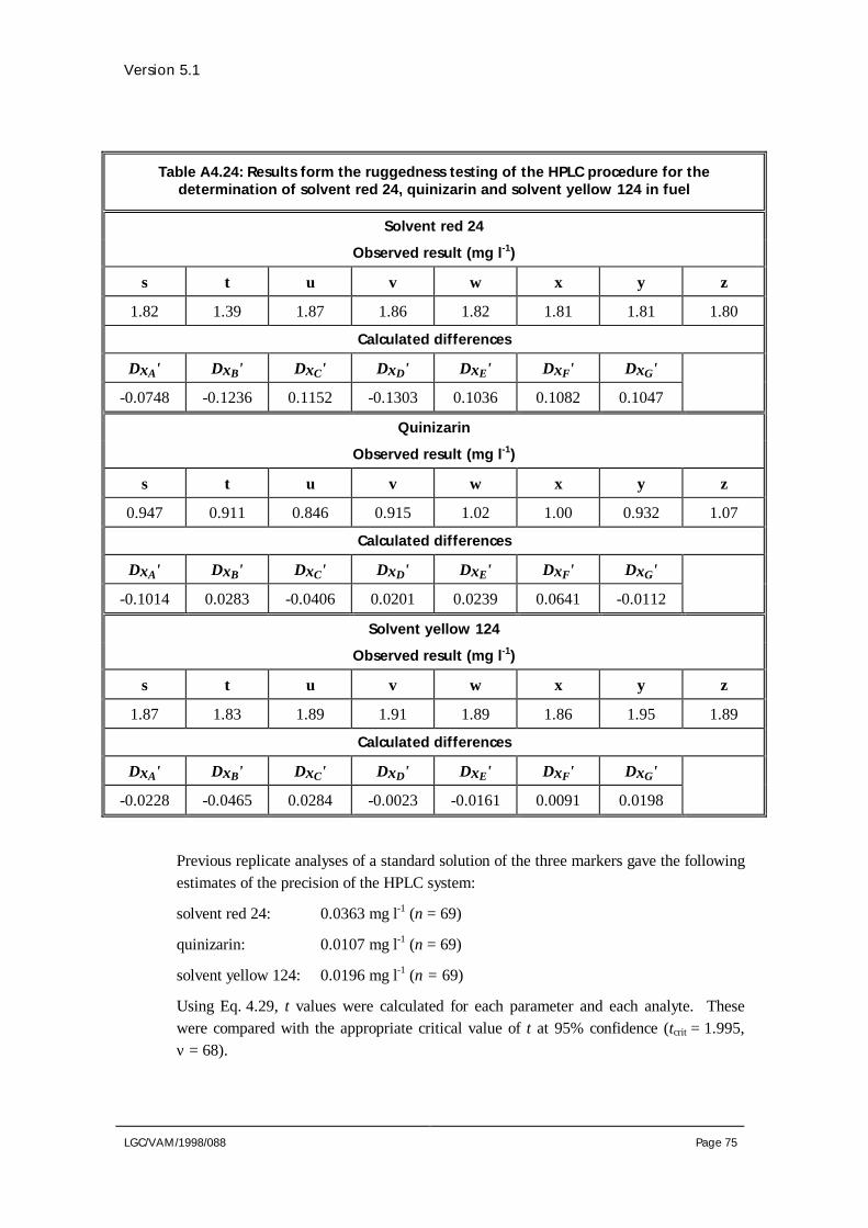
Version 5.1


Table A4.24: Results form the ruggedness testing of the HPLC procedure for thedetermination of solvent red 24, quinizarin and solvent yellow 124 in fuel

Solvent red 24


s t u v w x y z

1.82 1.39 1.87 1.86 1.82 1.81 1.81 1.80



-0.0748 -0.1236 0.1152 -0.1303 0.1036 0.1082 0.1047

Quinizarin


s t u v w x y z

0.947 0.911 0.846 0.915 1.02 1.00 0.932 1.07



-0.1014 0.0283 -0.0406 0.0201 0.0239 0.0641 -0.0112

Solvent yellow 124


s t u v w x y z

1.87 1.83 1.89 1.91 1.89 1.86 1.95 1.89



-0.0228 -0.0465 0.0284 -0.0023 -0.0161 0.0091 0.0198

Previous replicate analyses of a standard solution of the three markers gave the followingestimates of the precision of the HPLC system:

solvent red 24: 0.0363 mg l-1 (n = 69)

quinizarin: 0.0107 mg l-1 (n = 69)

solvent yellow 124: 0.0196 mg l-1 (n = 69)

Using Eq. 4.29, t values were calculated for each parameter and each analyte. Thesewere compared with the appropriate critical value of t at 95% confidence (tcrit = 1.995,ν = 68).

Version 5.1


Solvent red 24

All the parameters studied had a significant effect on the concentration of solvent red 24observed. The relevant uncertainties were calculated using the procedure outlined inSection 4.3.3.3.

Flow rate

In the ruggedness test the flow rate was varied by 0.4 ml min-1. This resulted in adifference of -0.1236 mg l-1. The sensitivity coefficient, cB', is therefore 0.309. Theuncertainty in the flow rate was estimated as 0.00173 ml min-1 (see section on all-transretinol ruggedness test). The uncertainty, u(y(xB')), is therefore 0.000535 mg l-1.

Injection volume

The method specifies an injection volume of 50 µl. The uncertainty associated with thiswas estimated as 0.75 µl (see all-trans retinol ruggedness test). The sensitivitycoefficient, cC', was calculated as 0.00576. The uncertainty, u(y(xC')), is therefore0.00432 mg l-1.

Column temperature

During routine use of the method, the column is thermostatted at 30°C. The uncertaintyassociated with this was estimated as ±1°C (see section on all-trans retinol ruggednesstest). In the ruggedness test the temperature was varied from 25°C to 35°C whichresulted in a difference of 0.1303 mg l-1. The sensitivity coefficient is therefore 0.01303and the uncertainty, u(y(xD')), is 0.00752 mg l-1.

Channel A wavelength

The wavelength for detector channel A is specified in the method as 475 nm. Theuncertainty associated with this was estimated as ±2 nm (assuming a rectangulardistribution). In the ruggedness study, a change in wavelength of 20 nm resulted in adifference of 0.1036 mg l-1. The uncertainty, u(y(xE')), is therefore 0.00598 mg l-1.

Channel B wavelength

The wavelength for detector channel B is specified in the method as 500 nm. In theruggedness study a change of 20 nm resulted in a difference of 0.1047 mg l-1. Theuncertainty is therefore 0.00604 mg l-1.

All the above uncertainties were converted to relative standard deviations by dividing by1.92 mg l-1.

Two other parameters also had a significant effect on the method performance: the typeof acetonitrile used in the mobile phase and whether or not the mobile phase wasdegassed. The method was developed using HPLC grade acetonitrile. The ruggednesstest indicated that changing to far-UV grade results in a lower recovery. The method

Version 5.1


protocol will therefore specify that for routine use, HPLC grade must be used. Theruggedness test also indicated that not degassing the mobile phase causes a reduction inrecovery. The method was developed using degassed mobile phase, and the methodprotocol will specify that this must be the case during future use of the method. As thesetwo parameters are being controlled in the method protocol, uncertainty terms have notbeen included.

Quinizarin

The results of the ruggedness test indicated that the following parameters have asignificant effect on the method performance:

Flow rate

Using the procedure discussed in the case of solvent red 24, the uncertainty wascalculated as 0.000122 mg l-1.

Injection volume

The uncertainty was calculated as 0.00152 mg l-1 (see solvent red 24 example).

Column temperature



Following the solvent red 24 example, the uncertainty was calculated as 0.00138 mg l-1.

As in the case of solvent red 24, no additional uncertainties associated with the grade ofacetonitrile used and the degassing of the mobile phase were included.


The ruggedness test indicated that this parameter does not have a significant effect on theresult of the analysis. The uncertainty was therefore evaluated using Eq. 4.30. δreal andδtest are equal to 4 nm and 20 nm respectively. The uncertainty was therefore calculatedas 0.00154 mg l-1.

All the uncertainties were converted to relative standard deviations by dividing by0.909 mg l-1.

Version 5.1


Solvent yellow 124

The results of the ruggedness test indicated that the following parameters have asignificant effect on the method performance:

Flow rate


Injection volume


As in the case of solvent red 24 and quinizarin, no additional uncertainties associatedwith the grade of acetonitrile used and the degassing of the mobile phase were included.

The results of the study indicated that remaining parameters do not have a significanteffect on the method performance. The uncertainty was therefore calculated usingEq. 4.30 which gives 0.0141 × (δtrue/δtest).

Column temperature

δtrue and δtest are equal to 2°C and 10°C respectively. The uncertainty is therefore0.00282 mg l-1.


δtrue and δtest are equal to 4 nm and 20 nm respectively. The uncertainty is therefore0.00282 mg l-1.


As in the case of the channel A wavelength, the uncertainty was calculated as0.00282 mg l-1.

The above uncertainties were converted to relative standard deviations by dividing by2.35 mg l-1.

Remaining sources of uncertainty

As discussed in Section A4.1.4 the uncertainties associated with a number of parameters,such as the calibration of the pipette used to dispense the samples, have not yet beenconsidered. However, as these uncertainties are generally small, no additionalcontributions to the uncertainty budget have been included.

Version 5.1


A4.2.5 Calculation of combined and expanded uncertainties

Table A4.25 summarises the magnitudes of the individual uncertainty components for the threemakers.

Table A4.25: Uncertainty budget for the determination of markers in oil

Standard uncertainties as relative standard deviations

Parameter Solvent red 24(0.04 - 4 mg l-1)

Quinizarin(0.04 - 2 mg l-1)

Solvent yellow(1.2 - 5 mg l-1)

Precision u(P) 0.0414 0.0788 0.0114

Recovery u(R) 0.0415 0.0974 0.0187

Brand of cartridge u(y(xA)) 0.0257 0.0190 0.00848

Sample volume u(y(xB)) 0.00367 0.00394 0.00360

Rate of elution of oilwith hexane

u(y(xC)) 0.00257 0.00767 0.000848

Volume of hexane wash u(y(xD)) 0.00111 0.00195 0.000957

Concentration ofbutan-1-ol/hexane

u(y(xE)) 0.00128 0.000951 0.000424

Volume ofbutan-1-ol/hexane

u(y(xF)) 0.000514 0.000380 0.000340

Evaporationtemperature

u(y(xG)) 0.00856 0.00480 0.00283

Flow rate u(y(xB')) 0.000279 0.000134 0.000855

Injection volume u(y(xC')) 0.00225 0.00167 0.000455

Column temperature u(y(xD')) 0.00392 0.00128 0.00120

Detector channel Awavelength

u(y(xE')) 0.00311 0.00152 0.00120

Detector channel Bwavelength

u(y(xG')) 0.00315 0.00169 0.00120

For all three analytes, the sources of uncertainty were considered to be proportional toanalyte concentration. The combined uncertainty was therefore calculated using Eq. 5.1:

solvent red 24: u(y)/y = 0.065

quinizarin: u(y)/y = 0.13

solvent yellow 124: u(y)/y = 0.024

Version 5.1


Table A4.26 to Table A4.28 gives standard and expanded uncertainties for typicalconcentrations of the three markers. The expanded uncertainties were calculated using acoverage factor of k = 2 which gives a confidence level of approximately 95%.

Table A4.26: Standard and expanded uncertainty estimates forthe determination of solvent red 24 in oil

Concentration(mg l-1)

Standarduncertainty

(mg l-1)

Relativestandard

uncertainty

Expandeduncertainty

(mg l-1)

0.04 0.0026 0.065 0.0052

1.5 0.098 0.065 0.20

2 0.13 0.065 0.26

4 0.26 0.065 0.52

Table A4.27: Standard and expanded uncertainty estimates forthe determination of quinizarin in oil


Standarduncertainty

(mg l-1)

Relativestandard

uncertainty

Expandeduncertainty

(mg l-1)

0.04 0.0052 0.13 0.010

1.0 0.13 0.13 0.26

1.5 0.19 0.13 0.39

2 0.26 0.13 0.52

Table A4.28: Standard and expanded uncertainty estimates forthe determination of solvent yellow 124 in oil


Standarduncertainty

(mg l-1)

Relativestandard

uncertainty

Expandeduncertainty

(mg l-1)

1.5 0.036 0.024 0.072

2 0.048 0.024 0.096

4 0.096 0.024 0.19

5 0.12 0.024 0.24

Version 5.1


Comments on uncertainty budget

Solvent red 24 and solvent yellow 124

In the case of solvent red 24 and solvent yellow 124, the significant contributions to theuncertainty budget arose from overall precision and recovery, and the brand of the solidphase extraction cartridge used. If a reduction in the overall uncertainty of the methodwas required, useful approaches would be to specify a particular brand of cartridge in themethod protocol, or to adopt matrix specific recovery corrections for test samples.

Quinizarin

The combined uncertainty for quinizarin, which is significantly greater than thatcalculated for the other markers, is dominated by the precision and recovery terms. Theresults of the precision study indicated variable method performance across differentmatrices and analyte concentrations. The uncertainty, u(Rs), associated with the variationin recovery from sample to sample was the major contribution to the recoveryuncertainty, u(R). This was due to the fact that the recoveries obtained for matrix B weregenerally higher than those obtained for matrices A and C. However, in this study, asingle uncertainty estimate for all the matrices and analyte concentrations studied wasrequired. It was therefore necessary to use “worst case” estimates of the uncertainties forprecision and recovery to adequately cover all sample types. If this estimate was found tobe unsatisfactory for future applications of the method, separate budgets could becalculated for individual matrices and concentration ranges.

Version 5.1


Annex 5: Proforma for documentinguncertainty

Page..........of..........

Uncertainty Budget

MethodTitle:

Ref:

Scope:

Sources of Uncertainty

1. Precision

Samples analysed

Matrix Concentration No.replicates

Standarddeviation

Analyst/date

u(P)

Page..........of..........

Uncertainty Budget

Method Title: Ref:

2. Trueness

Samples analysed

Matrix (CRM/spike?) Concentration No.replicates

Result Recovery Analyst/date

Rm u Rm( ) Rm differentfrom 1?

Correctionapplied?

u Rm( )' u(Rs) u(Rs) Rrep

u(Rrep) R u(R)

Page..........of..........

Uncertainty Budget

MethodTitle:

Ref:

3. Other

Source of Uncertainty StandardUncertainty

Method of evaluation Analyst/date

Combined standarduncertainty

Expanded uncertainty

Coverage factor applied andlevel of confidence

Prepared by: Date:

Version 5.1


Annex 6: References1 Guide to the Expression of Uncertainty in Measurement, ISO, Geneva, Switzerland 1993.

ISBN 92-67-10188-9.2 Eurachem: Quantifying Uncertainty in Analytical Measurement, Laboratory of the

Government Chemist, London, UK, 1995. ISBN 0-948926-08-2.3 The Fitness for Purpose of Analytical Methods, A Laboratory Guide to Method Validation

and Related Topics, Eurachem Guide, Edition 1, 1998. ISBN 0-948926-12-0.4 Practical Statistics for the Analytical Scientist, A Bench Guide, T. J. Farrant, Royal Society of

Chemistry, Cambridge, UK, 1997. ISBN 0-85404 442 6.5 V. J. Barwick and S. L. R. Ellison, Evaluating uncertainties associated with recovery, 1998,

VAM Technical Report, LGC/VAM/1998/052.6 V. J. Barwick and S. L. R. Ellison, Analyst, 1999, 124, 981.7 K. D. Bartle, A. A. Clifford, S. B. Hawthorne, J. J. Langenfeld, D. J. Miller, R. Robinson,

Journal of Supercritical Fluids, 1990, 3, 143.8 S. L. R. Ellison, Accred. Qual. Assur., 1998, 3, 95.9 S. L. R. Ellison and A. Williams in The use of recovery factors in trace analysis, M. Parkany

(Ed), Royal Society of Chemistry, Cambridge, UK, 1996. ISBN 0-85404-736-0.10 Statistical Manual of the Association of Official Analytical Chemists, W. J. Youden and E. H.

Steiner, Association of Official Analytical Chemist, Arlington, VA, 1975.ISBN 0-935584-15-3.

11 R. L. Plackett and J. P. Burman, Biometrika, 33, 305, 1946.12 Y. Vander Heyden, K. Luypaert, C. Hartmann, D. L. Massart, J. Hoogmartens, J. De Beer,

Anal. Chim. Acta, 1995, 312, 245.13 ISO 9004-4:1993, Total Quality Management Part 2. Guidelines for quality improvement.14 S. L. R. Ellison, V. J. Barwick, Accred. Qual. Assur., 1998, 3, 101.15 S. L. R. Ellison, V. J. Barwick, Analyst, 1998, 123, 1387.16 ISO 3534-1:1993. Statistics - Vocabulary and Symbols - Part 1: Probability and general

statistical terms.17 International Vocabulary of basic and general standard terms in Metrology, ISO, Geneva,

Switzerland 1993. ISBN 92-67-10175-1.18 V. J. Barwick, S. L. R. Ellison, Anal Comm., 1998, 35,377.19 ISO 5725:1994 Accuracy (Trueness and Precision) of Measurement Methods and Results.

ISO, Geneva, Switzerland.

Version 5.1


Index

BBias • 13, 37

CCalibration certificates • 25Cause and effect

analysis • 7diagram • 34

Coverage factor • 31, 37Critical value • 37

DDegrees of freedom • 37

EExpanded uncertainty

calculating • 31, 54definition • 37reporting • 33

FF-test

application • 10definition • 38

MMean recovery • 13, 16Measurement uncertainty

background • 1budget • 40, 53, 79definition • 38documentation • 33, 82

PPlackett-Burman experimental design • 26Precision

definition • 38

experiments • 8–13, 43, 58pooling estimates • 11, 43

Published data • 25

RRecovery

definition • 38experiments • 13–24, 44, 62uncertainty • 13–24

Rectangular distribution • 36Reference materials

use of • 16, 44, 62Relative standard deviation • 39Ruggedness test

application • 26–29, 46, 68design • 26

SSample standard deviation • 39Sensitivity coefficient

definition • 39estimation • 29

Significance testsapplication • 10, 21, 28definition • 39

Standard deviation of the mean • 40Standard uncertainty

calculating • 36combined • 30, 53definition • 40reporting • 33

TTrueness

definition • 40experiments • 13–24, 44, 62

t-testapplication • 21, 27definition • 39

vam project 3.2.1 development and harmonisation of measurement uncertainty...

Documents