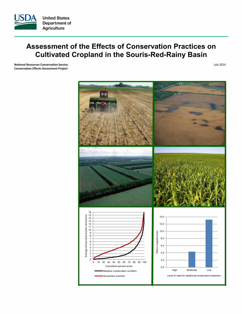
Assessment of the Effects of Conservation Practices on Cultivated Cropland in the Souris-Red-Rainy Basin

National Resources Conservation Service July 2014 Conservation Effects Assessment Project

0123456789

10111213141516

0 10 20 30 40 50 60 70 80 90 100

Aver

age

annu

al w

ind

eros

ion

(tons

/acr

e)

Cumulative percent acres

Baseline conservation condition

No-practice scenario

0.0

2.0

4.0

6.0

8.0

10.0

12.0

14.0

High Moderate Low

Mill

ion

crop

ped

acre

s

Level of need for additional conservation treatment

This page intentionally left blank.

Cover photos by (clockwise from top left) unknown, Don Poggensee, unknown, Scott Bauer, USDA Natural Resources Conservation Service

CEAP—Strengthening the science base for natural resource conservation The Conservation Effects Assessment Project (CEAP) was initiated by USDA’s Natural Resources Conservation Service (NRCS), Agricultural Research Service (ARS), and Cooperative State Research, Education, and Extension Service (CSREES—now National Institute of Food and Agriculture [NIFA]) in response to a general call for better accountability of how society would benefit from the 2002 Farm Bill’s substantial increase in conservation program funding (Mausbach and Dedrick 2004). The original goals of CEAP were to estimate conservation benefits for reporting at the national and regional levels and to establish the scientific understanding of the effects and benefits of conservation practices at the watershed scale. As CEAP evolved, the scope was expanded to provide research and assessment on how to best use conservation practices in managing agricultural landscapes to protect and enhance environmental quality. CEAP activities are organized into three interconnected efforts: • Bibliographies, literature reviews, and scientific workshops to establish what is known about the

environmental effects of conservation practices at the field and watershed scale. • National and regional assessments to estimate the environmental effects and benefits of conservation practices

on the landscape and to estimate conservation treatment needs. The four components of the national and regional assessment effort are Cropland; Wetlands; Grazing lands, including rangeland, pastureland, and grazed forest land; and Wildlife.

• Watershed studies to provide in-depth quantification of water quality and soil quality impacts of conservation

practices at the local level and to provide insight on what practices are the most effective and where they are needed within a watershed to achieve environmental goals.

Research and assessment efforts were designed to estimate the effects and benefits of conservation practices through a mix of research, data collection, model development, and model application. A vision for how CEAP can contribute to better and more effective delivery of conservation programs in the years ahead is addressed in Maresch, Walbridge, and Kugler (2008). Additional information on the scope of the project can be found at http://www.nrcs.usda.gov/wps/portal/nrcs/main/national/technical/nra/ceap/pub/.

1

This report was prepared by the Conservation Effects Assessment Project (CEAP) Cropland Modeling Team and published by the United States Department of Agriculture (USDA), Natural Resources Conservation Service (NRCS). The modeling team consists of scientists and analysts from NRCS, the Agricultural Research Service (ARS), Texas AgriLife Research, and the University of Massachusetts. Natural Resources Conservation Service, USDA

Daryl Lund, Project Coordinator, Beltsville, MD, Soil Scientist Jay D. Atwood, Temple, TX, Agricultural Economist Joseph K. Bagdon, Amherst, MA, Agronomist and Pest Management Specialist Jim Benson, Beltsville, MD, Program Analyst (retired) Jeff Goebel, Beltsville, MD, Statistician (retired) Kevin Ingram, Beltsville, MD, Agricultural Economist Mari-Vaughn V. Johnson, Temple, TX, Agronomist Robert L. Kellogg, Beltsville, MD, Agricultural Economist (retired, Earth Team Volunteer) Jerry Lemunyon, Fort Worth, TX, Agronomist and Nutrient Management Specialist (retired, Earth Team Volunteer) Lee Norfleet, Temple, TX, Soil Scientist Evelyn Steglich, Temple, TX, Natural Resource Specialist

Agricultural Research Service, USDA, Grassland Soil and Water Research Laboratory, Temple, TX

Jeff Arnold, Agricultural Engineer Mike White, Agricultural Engineer

Blackland Center for Research and Extension, Texas AgriLife Research, Temple, TX

Tom Gerik, Director Santhi Chinnasamy, Agricultural Engineer Mauro Di Luzio, Research Scientist Arnold King, Resource Conservationist David C. Moffitt, Environmental Engineer Kannan Narayanan, Agricultural Engineer Theresa Pitts, Programmer Xiuying (Susan) Wang, Agricultural Engineer Jimmy Williams, Agricultural Engineer

University of Massachusetts Extension, Amherst, MA Stephen Plotkin, Water Quality Specialist

The study was conducted under the direction of Mike Golden, Deputy Chief for Soil Science and Resource Assessment, Michele Laur, Director for Resource Assessment Division, and Douglas Lawrence, Wayne Maresch, William Puckett, and Maury Mausbach, former Deputy Chiefs for Soil Survey and Resource Assessment, NRCS. Executive support was provided by the current NRCS Chief, Jason Weller, and former NRCS Chiefs Dave White, Arlen Lancaster, and Bruce Knight. Acknowledgements The team thanks Alex Barbarika, Rich Iovanna, and Skip Hyberg USDA-Farm Service Agency, for providing data on Conservation Reserve Program (CRP) practices and making contributions to the report; Harold Coble and Danesha Carley, North Carolina State University, for assisting with the analysis of the integrated pest management (IPM) survey data; Dania Fergusson, Eugene Young, and Kathy Broussard, USDA-National Agricultural Statistics Service, for leading the survey data collection effort; Mark Siemers and Todd Campbell, CARD, Iowa State University, for providing I-APEX support; NRCS field offices for assisting in collection of conservation practice data; Dean Oman, USDA-NRCS, Beltsville, MD, for geographic information systems (GIS) analysis support; Melina Ball, Texas AgriLife Research, Temple, TX, for HUMUS graphics support; Peter Chen, Susan Wallace, George Wallace, and Karl Musser, Paradigm Systems, Beltsville, MD, for graphics support, National Resources Inventory (NRI) database support, Web site support, and calculation of standard errors; and many others who provided advice, guidance, and suggestions throughout the project. The team also acknowledges the many helpful and constructive suggestions and comments by reviewers who participated in the peer review of earlier versions of the report.

2

Foreword The United States Department of Agriculture has a rich tradition of working with farmers and ranchers to enhance agricultural productivity and environmental protection. Conservation pioneer Hugh Hammond Bennett worked tirelessly to establish a nationwide Soil Conservation Service along with a system of Soil and Water Conservation Districts. The purpose of these entities, now as then, is to work with farmers and ranchers and help them plan, select, and apply conservation practices to enable their operations to produce food, forage, and fiber while conserving the Nation’s soil and water resources. USDA conservation programs are voluntary. Many provide financial assistance to producers to help encourage adoption of conservation practices. Others provide technical assistance to design and install conservation practices consistent with the goals of the operation and the soil, climatic, and hydrologic setting. By participating in USDA conservation programs, producers are able to— • install structural practices such as riparian buffers, grass filter strips, terraces, grassed waterways, and contour farming to reduce

erosion, sedimentation, and nutrients leaving the field; • adopt conservation systems and practices such as conservation tillage, comprehensive nutrient management, integrated pest

management, and irrigation water management to conserve resources and maintain the long-term productivity of crop and pasture land; and

• retire land too fragile for continued agricultural production by planting and maintaining on them grasses, trees, or wetland vegetation.

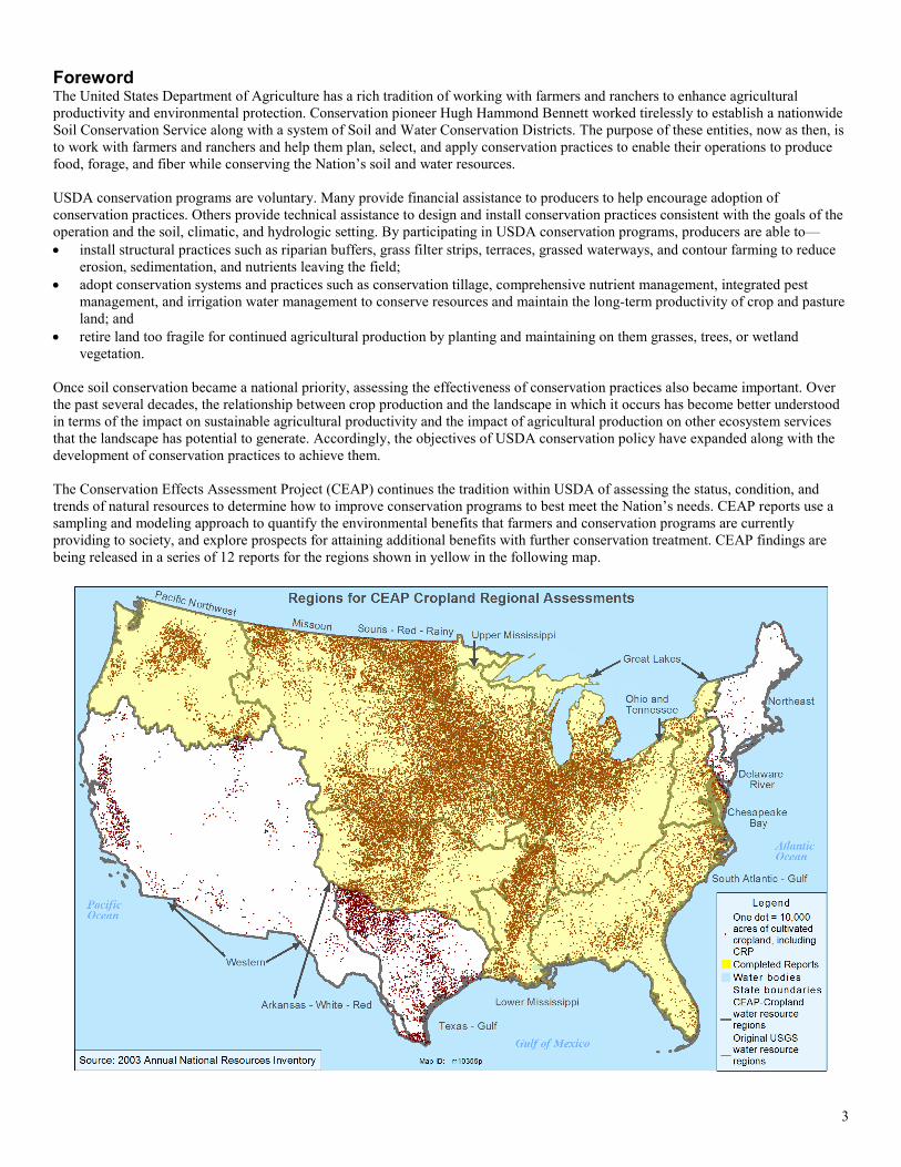
Once soil conservation became a national priority, assessing the effectiveness of conservation practices also became important. Over the past several decades, the relationship between crop production and the landscape in which it occurs has become better understood in terms of the impact on sustainable agricultural productivity and the impact of agricultural production on other ecosystem services that the landscape has potential to generate. Accordingly, the objectives of USDA conservation policy have expanded along with the development of conservation practices to achieve them. The Conservation Effects Assessment Project (CEAP) continues the tradition within USDA of assessing the status, condition, and trends of natural resources to determine how to improve conservation programs to best meet the Nation’s needs. CEAP reports use a sampling and modeling approach to quantify the environmental benefits that farmers and conservation programs are currently providing to society, and explore prospects for attaining additional benefits with further conservation treatment. CEAP findings are being released in a series of 12 reports for the regions shown in yellow in the following map.

3

Assessment of the Effects of Conservation Practices on Cultivated Cropland in the Souris-Red-Rainy Basin Contents Page Executive Summary 6 Chapter 1: Land Use and Agriculture in the Souris-Red-Rainy Basin

Land Use 11 Agriculture 11 Watersheds 14

Chapter 2: Overview of Sampling and Modeling Approach

Scope of Study 16 Sampling and Modeling Approach 16 The NRI and the CEAP Sample 17 The NRI-CEAP Cropland Survey 18 Estimated Acres 18 Cropping Systems in the Souris-Red-Rainy Basin 19 Simulating the Effects of Weather 20

Chapter 3: Evaluation of Conservation Practice Use—the Baseline Conservation Condition

Historical Context for Conservation Practice Use 22 Summary of Practice Use 22 Structural Conservation Practices 23 Residue and Tillage Management Practices 25 Conservation Crop Rotation 25 Cover Crops 28 Irrigation Management Practices 28 Nutrient Management Practices 28 Pesticide Management Practices 33 Conservation Cover Establishment 35

Chapter 4: Onsite (Field-Level) Effects of Conservation Practices

The Field-Level Cropland Model—APEX 36 Simulating the No-Practice Scenario 37 Effects of Practices on Fate and Transport of Water 43 Effects of Practices on Wind Erosion 48 Effects of Practices on Water Erosion and Sediment Loss 50 Effects of Practices on Soil Organic Carbon 54 Effects of Practices on Nitrogen Loss 57 Effects of Practices on Phosphorus Loss 64 Effects of Practices on Pesticide Residues and Environmental Risk 68

Chapter 5: Assessment of Conservation Treatment Needs

Conservation Treatment Levels 74 Inherent Vulnerability Factors 79 Evaluation of Conservation Treatment 86

Chapter 6: Offsite Water Quality Effects of Conservation Practices

The National Water Quality Model—HUMUS/SWAT 97 Source Loads and Instream Loads 102 Modeling Land Use 105 Loads Delivered from Cultivated Cropland to Rivers and Streams within the Region 106 Instream Loads from All Sources Exported from the Region 113

4

Chapter 7: Summary of Findings

Field Level Assessment 118 Loads Delivered to Rivers and Streams within the Region 120 Instream Loads from All Sources Exported from the Region 120

References 121 Appendix A: Estimates of Margins of Error for Selected Acre Estimates 123 Appendix B: Model Simulation Results for Subregions 0901 and 0902 in the Souris-Red-Rainy Basin 126 Documentation Reports There are a series of documentation reports and associated publications by the modeling team posted on the CEAP website at: http://www.nrcs.usda.gov/wps/portal/nrcs/main/national/technical/nra/ceap/pub/. (Click on “full list of modeling documentation reports.”) Included are the following reports that provide details on the modeling and databases used in this report:

• 0BThe HUMUS/SWAT National Water Quality Modeling System and Databases • 1BCalibration and Validation of CEAP-HUMUS • Delivery Ratios Used in CEAP Cropland Modeling • APEX Model Validation for CEAP • Pesticide Risk Indicators Used in CEAP Cropland Modeling • Integrated Pest Management (IPM) Indicator Used in CEAP Cropland Modeling • NRI-CEAP Cropland Survey Design and Statistical Documentation • Transforming Survey Data to APEX Model Input Files • Modeling Structural Conservation Practices for the Cropland Component of the National Conservation Effects Assessment

Project • APEX Model Upgrades, Data Inputs, and Parameter Settings for Use in CEAP Cropland Modeling • APEX Calibration and Validation Using Research Plots in Tifton, Georgia • The Agricultural Policy Environmental EXtender (APEX) Model: An Emerging Tool for Landscape and Watershed

Environmental Analyses • The Soil and Water Assessment Tool: Historical Development, Applications, and Future Research Directions • Historical Development and Applications of the EPIC and APEX Models • Assumptions and Procedures for Simulating the Natural Vegetation Background Scenario for the CEAP National Cropland

Assessment • Manure Loadings Used to Simulate Pastureland and Hayland in CEAP HUMUS/SWAT modeling • Adjustment of CEAP Cropland Survey Nutrient Application Rates for APEX Modeling

5

Assessment of the Effects of Conservation Practices on Cultivated Cropland in the Souris-Red-Rainy Basin

Executive Summary

Agriculture in the Souris-Red-Rainy Basin The Souris-Red-Rainy Basin consists of the drainage along the border with Canada in North Dakota and Minnesota that ultimately discharges into Lake Winnipeg and Hudson Bay in Canada. A small part of the northeast corner of South Dakota is also included in the basin. The basin extends into Canada but covers 59,460 square miles (38 million acres) within the United States. This study only includes the portion of the drainage area that is in the United States. Land cover in the basin is dominated by cultivated cropland in the west and forestland and wetlands in the east. Cultivated cropland is the dominant land use in two of the subregions. The Souris River drainage within the United States has 3.6 million acres of cultivated cropland, accounting for 62 percent of the total area in the subregion. The Red River drainage within the United States has 16.6 million acres of cultivated cropland, accounting for 66 percent of the total area within the subregion. The third subregion—the Rainy River and Lake of the Woods drainage within the United States—has less than 100,000 acres of cultivated cropland. Urban areas make up only about 4 percent of the basin. The major metropolitan area within the basin is Fargo, ND. The 2007 Census of Agriculture reported 30,330 farms in the Souris-Red-Rainy Basin, about 1 percent of the total number of farms in the United States. About 81 percent of Souris-Red-Rainy Basin farms primarily raise crops, about 14 percent are primarily livestock operations, and the remaining 5 percent produce a mix of livestock and crops. The Souris-Red-Rainy Basin accounted for about 3 percent of all U.S. crop sales in 2007, totaling $4.8 billion. Wheat, soybeans, and corn are the principal crops grown, accounting for 68 percent of harvested crop acreage in 2007. Barley, sugarbeets, alfalfa hay, and tame and wild hay are also important crops in the region. Farmers in the region produced 28 percent of all barley harvested in the United States in 2007, 19 percent of the national sugarbeet crop, and 13 percent of the national wheat crop. Focus of CEAP Study Is on Edge-Of-Field Losses from Cultivated Cropland The primary focus of the CEAP Souris-Red-Rainy Basin study is on the 20 million acres of cultivated cropland, including land in long-term conserving cover. The study was designed to quantify the effects of conservation practices commonly used on cultivated cropland in the Souris-Red-Rainy Basin during 2003–06 and evaluate the need for additional conservation treatment in the region on the basis of edge-of-field losses. The assessment uses a statistical sampling and modeling approach to estimate the effects of conservation practices. The National Resources Inventory, a statistical survey of conditions and trends in soil, water, and related resources on U.S. non-Federal land conducted by USDA’s Natural Resources Conservation Service, provides the statistical framework. Physical process simulation models were used to estimate the effects of conservation practices in use during the period 2003–06. Information on farming activities and conservation practices was obtained primarily from a farmer survey conducted as part of the study. The assessment includes not only practices associated with Federal conservation programs but also the conservation efforts of States, independent organizations, and individual landowners and farm operators. The analysis assumes that structural practices (such as buffers, terraces, and grassed waterways) reported in the farmer survey or obtained from other sources were appropriately designed, installed, and maintained. The assessment was done using a common set of criteria and protocols applied to all regions in the country to provide a systematic, consistent, and comparable assessment at the national level. The sample size of the farmer survey—18,700 sample points nationally with 476 sample points in the Souris-Red-Rainy Basin—is sufficient for reliable and defensible reporting for the two subregions where the cultivated cropland is the dominant land use—the

6

Souris River subregion and the Red River subregion. Because so few acres of cultivated cropland are in the Rainy River subregion, no survey samples were obtained for this region. Thus, the assessment of the effects of conservation practices and conservation treatment needs reported in this study apply only to the Souris and Red River subregions. Voluntary, Incentives-Based Conservation Approaches Are Achieving Results Results from the farmer survey show that farmers in the Souris-Red-Rainy Basin have made significant progress in reducing sediment, nutrient, and pesticide losses from farm fields through conservation practice adoption. Conservation Practice Use The farmer survey found, for the period 2003–06, that producers use either residue and tillage management practices or structural practices, or both, on 89 percent of the cropped acres. • Structural practices for controlling water erosion are in use on 18 percent of cropped acres. Thirteen percent of

cropped acres are designated as highly erodible land; structural practices designed to control water erosion are in use on 23 percent of these acres.

• Structural practices for controlling wind erosion are in use on 20 percent of cropped acres, including 26 percent of highly erodible land.

• Reduced tillage is common in the region; 72 percent of the cropped acres meet criteria for either no-till (17 percent) or mulch till (55 percent). All but 12 percent of the acres have evidence of some kind of reduced tillage on at least one crop in the rotation.

The use of nutrient management practices is more widespread in this region than other regions. The farmer survey found that the majority of acres have evidence of some nitrogen or phosphorus management. For example: • About 64 percent of cropped acres meet criteria for timing of nitrogen applications on all crops in the rotation,

78 percent meet criteria for method of application, and 71 percent meet criteria for rate of application. An additional 1 percent of cropped acres have no nitrogen applied.

• About 79 percent of cropped acres meet criteria for timing of phosphorus applications on all crops in the rotation, 83 percent meet criteria for method of application, and 55 percent meet criteria for rate of application. An additional 2 percent of cropped acres have no phosphorus applied.

There was less evidence, however, of consistent use of appropriate rates, timing, and method of nutrient application on each crop in every year of production. • Appropriate nitrogen application rates, timing of application, and application method for all crops during every

year of production are in use on 38 percent of cropped acres. • Good phosphorus management practices (appropriate rate, timing, and method) are in use on 43 percent of the

acres on all crops during every year of production. • About 25 percent of cropped acres meet nutrient management criteria for both nitrogen and phosphorus

management, including acres with no nutrient applications. Land in long-term conserving cover, as represented by enrollment in the CRP General Signup, consists of 2.3 million acres in the region, of which 29 percent is highly erodible land. Conservation Accomplishments at the Field Level Compared to a model scenario without conservation practices, field-level model simulations on cropped acres showed that conservation practice use during the period 2003–06 has— • reduced wind erosion by 52 percent; • reduced waterborne sediment loss from fields by 43 percent; • reduced nitrogen lost with windborne sediment by 45 percent; • reduced nitrogen lost with surface runoff (attached to sediment and in solution) by 67 percent; • reduced nitrogen loss in subsurface flows by 71 percent; • reduced total phosphorus loss (all loss pathways) from fields by 57 percent; and • reduced pesticide loss from fields to surface water, resulting in a 78-percent reduction in edge-of-field pesticide

risk (all pesticides combined) for aquatic ecosystems and a 74-percent reduction in edge-of-field surface water pesticide risk for humans.

7

In this region, conservation practices on cropped acres have a positive effect on soil organic carbon levels for most cropped acres. Conservation practice use in the region has resulted in an average annual gain in soil organic carbon of 77 pounds per acre per year on cropped acres. For land in long-term conserving cover (2.3 million acres), soil erosion and sediment loss have been almost completely eliminated. Compared to a cropped condition without conservation practices, total nitrogen loss has been reduced by 77 percent, total phosphorus loss has been reduced by 86 percent, and soil organic carbon has been increased by an average of 274 pounds per acre per year. If the 2003–06 level of conservation practice use is not maintained, some of these gains will be lost. Conservation Accomplishments at the Watershed Level Reductions in field-level losses due to conservation practices, including land in long-term conserving cover, are expected to reduce loads delivered from cultivated cropland to rivers and streams in the region. Edge-of-field losses of sediment, nitrogen, and phosphorus were incorporated into a national water quality model to estimate the extent to which conservation practices have reduced amounts of these contaminants delivered to rivers and streams throughout the region. Transport of sediment, nutrients, and pesticides from farm fields to streams and rivers involves a variety of processes and time-lags, and not all of the potential pollutants leaving fields contribute to loads delivered to rivers and streams. Model simulation results for the Souris and Red Rivers indicate that for the baseline conservation condition, sediment and nutrient loads delivered to rivers and streams from cultivated cropland sources per year, on average, are— • 371,000 tons of sediment (77 percent of loads from all sources); • 53.3 million pounds of nitrogen (83 percent of loads from all sources); and • 2.1 million pounds of phosphorus (57 percent of loads from all sources). Conservation practices in use on cultivated cropland in 2003–06, including land in long-term conserving cover, have reduced sediment and nutrient loads delivered to rivers and streams from cultivated cropland sources per year, on average, by 50 percent for sediment, 75 percent for nitrogen, and 52 percent for phosphorus. The effects of conservation practices are also estimated for instream loads from all sources. Conservation practices in use on cultivated cropland in 2003-06, including land in long-term conserving cover, have reduced annual instream loads from all sources delivered from the Souris River subregion, on average, by 20 percent for sediment 83 percent for nitrogen, and 33 percent for phosphorus. The percent reductions are similar for the Red River subregion. Conservation practices in use on cultivated cropland in 2003-06 have reduced annual instream loads from all sources delivered from the Red River subregion, on average, by 5 percent for sediment, 75 percent for nitrogen, and 38 percent for phosphorus.

Emerging technologies not evaluated in this study promise to provide even greater conservation benefits once their use becomes more widespread. These include— • innovations in implement design to enhance precise nutrient application and

placement, including variable rate technologies and improved manure application equipment;

• enhanced-efficiency nutrient application products such as slow or controlled-release fertilizers (for example: polymer-coated products, sulfur-coated products, etc.) and nitrogen stabilizers (for example: urease inhibitors and nitrification inhibitors);

• drainage water management that controls discharge of drainage water and treats contaminants, thereby reducing the levels of nitrogen and even some soluble phosphorus loss;

• constructed wetlands receiving surface water runoff and drainage water from farm fields prior to discharge to streams and rivers; and

8

Opportunities Exist to Further Reduce Sediment and Nutrient Losses from Cultivated Cropland The assessment of conservation treatment needs identifies significant opportunities to further reduce contaminant losses from farm fields. Simulation model results indicate that wind erosion is the principal conservation treatment need in this region. A total of 4.3 million acres need additional treatment for wind erosion, representing 25 percent of cropped acres in the region. These 4.3 million acres have an average wind erosion rate of 4.6 tons per acre per year and lose, on average, 18.8 pounds per acre of nitrogen and 3.2 pounds per acre of phosphorus with windborne sediment each year. Resource concerns related to water quality were not as pronounced in this region as in other regions of the country, in part because of the lower levels of precipitation, the short growing season, the preponderance of close grown crops in the cropping systems, and the widespread use of conservation practices throughout the region. Moreover, acres with a high or moderately high soil runoff or leaching potential represent a small minority of cropped acres in this region. No acres in the region exceeded the “acceptable levels” of loss for sediment (2 tons per acre per year), nitrogen in runoff (15 pounds per acre per year), and phosphorus (4 pounds per acre per year) based on the long-term average loss estimates. A small number of acres (about 300,000 acres, representing 2 percent of cropped acres) had average annual losses of nitrogen in subsurface flows above 25 pounds per acre per year, but these were not widespread enough to be detected as a significant conservation treatment need. The majority of cropped acres in this region—13.2 million acres, representing 75 percent of cropped acres—were determined to have a low level of conservation treatment need. Acres with a low level of need for conservation treatment consist of acres that are adequately treated with respect to the level of inherent vulnerability. In the Souris-Red-Rainy Basin, these 13.2 million acres have an average wind erosion rate of 1.5 tons per acre per year and lose (per acre per year, on average) only 0.05 ton of sediment by water erosion, 1.6 pounds of phosphorus, and 21 pounds of nitrogen. While gains can be attained by adding conservation practices to some of these acres with a low treatment need, additional conservation treatment would reduce average field losses by only a small amount. Most of the acres that need additional treatment for wind erosion are found in the Red River subregion. Twenty-eight percent of the cropped acres in this subregion (4.1 million acres) need additional treatment for wind erosion. Less than 300,000 acres need additional treatment in the Souris River subregion (9 percent of acres within subregion). These estimates of conservation treatment needs do not address ecological outcomes, nor were they specifically derived to attain Federal, State, or local water quality goals within the region. Ecosystem impacts related to water quality are specific to each water body. Water quality goals depend on the designated uses for each water body. The regional scale and statistical design of this study preclude assessment of the current state of the aquatic ecosystems. Conservation treatment needs, as reported here, were estimated to achieve “full treatment” from the field-level perspective, rather than to reduce instream loads to levels adequate for designated water uses. From this perspective, a field with adequate conservation treatment will have combinations of practices that address all the specific inherent vulnerability factors that determine the potential for sediment, nutrient, and pesticide losses. For purposes of this report, “full treatment” consists of a suite of practices that— • avoid or limit the potential for contaminant losses by using nutrient management practices (appropriate rate,

timing, and method) on all crops in the rotation; • control overland flow where needed; and • trap materials leaving the field using appropriate edge-of-field mitigation.

9

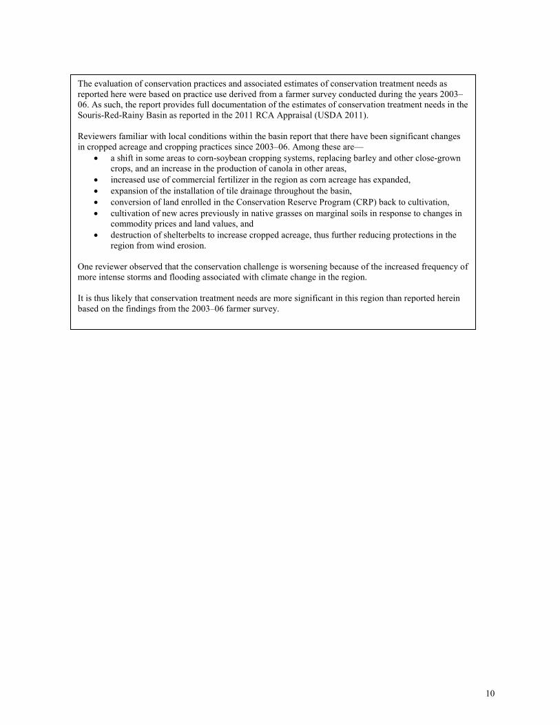
The evaluation of conservation practices and associated estimates of conservation treatment needs as reported here were based on practice use derived from a farmer survey conducted during the years 2003–06. As such, the report provides full documentation of the estimates of conservation treatment needs in the Souris-Red-Rainy Basin as reported in the 2011 RCA Appraisal (USDA 2011). Reviewers familiar with local conditions within the basin report that there have been significant changes in cropped acreage and cropping practices since 2003–06. Among these are—

• a shift in some areas to corn-soybean cropping systems, replacing barley and other close-grown crops, and an increase in the production of canola in other areas,

• increased use of commercial fertilizer in the region as corn acreage has expanded, • expansion of the installation of tile drainage throughout the basin, • conversion of land enrolled in the Conservation Reserve Program (CRP) back to cultivation, • cultivation of new acres previously in native grasses on marginal soils in response to changes in

commodity prices and land values, and • destruction of shelterbelts to increase cropped acreage, thus further reducing protections in the

region from wind erosion. One reviewer observed that the conservation challenge is worsening because of the increased frequency of more intense storms and flooding associated with climate change in the region. It is thus likely that conservation treatment needs are more significant in this region than reported herein based on the findings from the 2003–06 farmer survey.

10

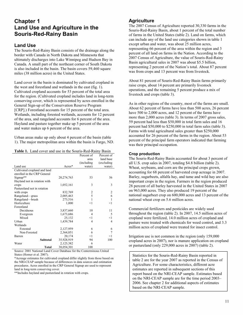
Chapter 1 Land Use and Agriculture in the Souris-Red-Rainy Basin Land Use The Souris-Red-Rainy Basin consists of the drainage along the border with Canada in North Dakota and Minnesota that ultimately discharges into Lake Winnipeg and Hudson Bay in Canada. A small part of the northeast corner of South Dakota is also included in the basin. The basin covers 59,460 square miles (38 million acres) in the United States. Land cover in the basin is dominated by cultivated cropland in the west and forestland and wetlands in the east (fig. 1). Cultivated cropland accounts for 53 percent of the total area for the region. (Cultivated cropland includes land in long-term conserving cover, which is represented by acres enrolled in the General Sign-up of the Conservation Reserve Program [CRP].) Forestland accounts for 15 percent of the total area. Wetlands, including forested wetlands, accounts for 12 percent of the area, and rangeland accounts for 6 percent of the area. Hayland and pasture together make up 5 percent of the area and water makes up 6 percent of the area. Urban areas make up only about 4 percent of the basin (table 1). The major metropolitan area within the basin is Fargo, ND. Table 1. Land cover and use in the Souris-Red-Rainy Basin

Land use Acres*

Percent of area

(including water)

Percent of land base

(excluding water)

Cultivated cropland and land enrolled in the CRP General Signup** 20,274,763 53 56 Hayland not in rotation with crops 1,052,161 3 3 Pastureland not in rotation with crops 832,769 2 2 Rangeland—grass 2,005,463 5 6 Rangeland—brush 273,516 1 1 Horticulture 1,000 <1 <1 Forestland

Deciduous 3,837,660 10 11 Evergreen 1,673,686 4 5 Mixed 25,132 <1 <1

Urban 1,439,784 4 4 Wetlands

Forested 2,127,959 6 6 Non-Forested 2,364,851 6 7

Barren 20,174 <1 <1 Subtotal 35,928,919 94 100

Water 2,125,382 6 Total 38,054,301 100

Source: 2001 National Land Cover Database for the Conterminous United States (Homer et al. 2007). *Acreage estimates for cultivated cropland differ slightly from those based on the NRI-CEAP sample because of differences in data sources and estimation procedures. Acres enrolled in the CRP General Signup are used to represent land in long-term conserving cover. **Includes hayland and pastureland in rotation with crops.

Agriculture The 2007 Census of Agriculture reported 30,330 farms in the Souris-Red-Rainy Basin, about 1 percent of the total number of farms in the United States (table 2). Land on farms, which can include any of the land use categories shown in table 1 except urban and water, was about 25 million acres, representing 66 percent of the area within the region and 3 percent of all land on farms in the Nation. According to the 2007 Census of Agriculture, the value of Souris-Red-Rainy Basin agricultural sales in 2007 was about $5.5 billion, representing 2 percent of the Nation’s total. About 87 percent was from crops and 13 percent was from livestock. About 81 percent of Souris-Red-Rainy Basin farms primarily raise crops, about 14 percent are primarily livestock operations, and the remaining 5 percent produce a mix of livestock and crops (table 3). As in other regions of the country, most of the farms are small. About 62 percent of farms have less than 500 acres, 26 percent have 500 to 2,000 acres, and 12 percent of the farms have more than 2,000 acres (table 3). In terms of 2007 gross sales, 59 percent had less than $50,000 in total farm sales and 16 percent had $50,000 to $250,000 in total farm sales (table 3). Farms with total agricultural sales greater than $250,000 accounted for 26 percent of the farms in the region. About 53 percent of the principal farm operators indicated that farming was their principal occupation. Crop production The Souris-Red-Rainy Basin accounted for about 3 percent of all U.S. crop sales in 2007, totaling $4.8 billion (table 2). Wheat, soybeans, and corn are the principal crops grown, accounting for 68 percent of harvested crop acreage in 2007. Barley, sugarbeets, alfalfa hay, and tame and wild hay are also important crops in the region. Farmers in the region produced 28 percent of all barley harvested in the United States in 2007 on 963,000 acres. They also produced 19 percent of the national sugarbeet crop on 600,000 acres and 13 percent of the national wheat crop on 5.6 million acres. Commercial fertilizers and pesticides are widely used throughout the region (table 2). In 2007, 14.5 million acres of cropland were fertilized, 14.0 million acres of cropland and pasture were treated with chemicals for weed control, and 3.3 million acres of cropland were treated for insect control. Irrigation use is not common in the region (only 159,000 cropland acres in 2007), nor is manure application on cropland or pastureland (only 229,000 acres in 2007) (table 2). .

Statistics for the Souris-Red-Rainy Basin reported in table 2 are for the year 2007 as reported in the Census of Agriculture. For some characteristics, different acre estimates are reported in subsequent sections of this report based on the NRI-CEAP sample. Estimates based on the NRI-CEAP sample are for the time period 2003–2006. See chapter 2 for additional aspects of estimates based on the NRI-CEAP sample.

11

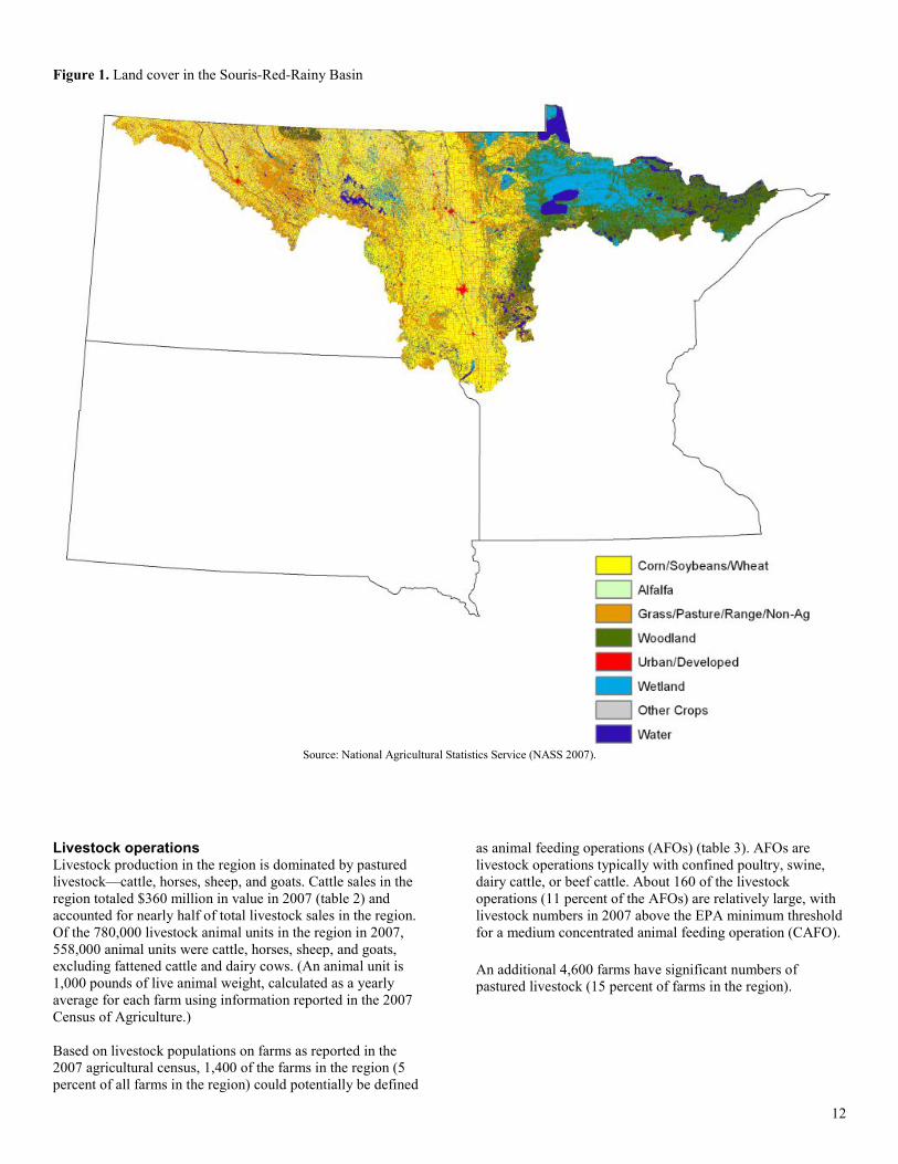
Figure 1. Land cover in the Souris-Red-Rainy Basin

Source: National Agricultural Statistics Service (NASS 2007).

Livestock operations Livestock production in the region is dominated by pastured livestock—cattle, horses, sheep, and goats. Cattle sales in the region totaled $360 million in value in 2007 (table 2) and accounted for nearly half of total livestock sales in the region. Of the 780,000 livestock animal units in the region in 2007, 558,000 animal units were cattle, horses, sheep, and goats, excluding fattened cattle and dairy cows. (An animal unit is 1,000 pounds of live animal weight, calculated as a yearly average for each farm using information reported in the 2007 Census of Agriculture.) Based on livestock populations on farms as reported in the 2007 agricultural census, 1,400 of the farms in the region (5 percent of all farms in the region) could potentially be defined

as animal feeding operations (AFOs) (table 3). AFOs are livestock operations typically with confined poultry, swine, dairy cattle, or beef cattle. About 160 of the livestock operations (11 percent of the AFOs) are relatively large, with livestock numbers in 2007 above the EPA minimum threshold for a medium concentrated animal feeding operation (CAFO). An additional 4,600 farms have significant numbers of pastured livestock (15 percent of farms in the region).

12

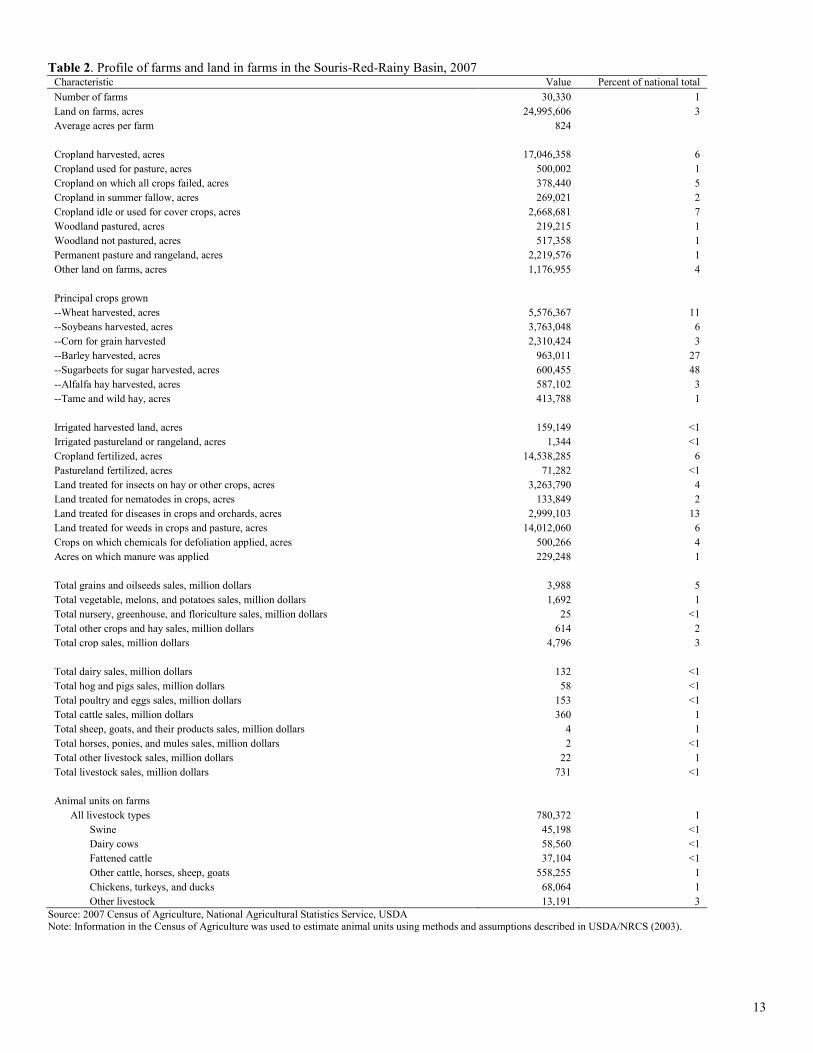
Table 2. Profile of farms and land in farms in the Souris-Red-Rainy Basin, 2007

Characteristic Value Percent of national total Number of farms 30,330 1 Land on farms, acres 24,995,606 3 Average acres per farm 824

Cropland harvested, acres 17,046,358 6 Cropland used for pasture, acres 500,002 1 Cropland on which all crops failed, acres 378,440 5 Cropland in summer fallow, acres 269,021 2 Cropland idle or used for cover crops, acres 2,668,681 7 Woodland pastured, acres 219,215 1 Woodland not pastured, acres 517,358 1 Permanent pasture and rangeland, acres 2,219,576 1 Other land on farms, acres 1,176,955 4

Principal crops grown --Wheat harvested, acres 5,576,367 11

--Soybeans harvested, acres 3,763,048 6 --Corn for grain harvested 2,310,424 3 --Barley harvested, acres 963,011 27 --Sugarbeets for sugar harvested, acres 600,455 48 --Alfalfa hay harvested, acres 587,102 3 --Tame and wild hay, acres 413,788 1

Irrigated harvested land, acres 159,149 <1 Irrigated pastureland or rangeland, acres 1,344 <1 Cropland fertilized, acres 14,538,285 6 Pastureland fertilized, acres 71,282 <1 Land treated for insects on hay or other crops, acres 3,263,790 4 Land treated for nematodes in crops, acres 133,849 2 Land treated for diseases in crops and orchards, acres 2,999,103 13 Land treated for weeds in crops and pasture, acres 14,012,060 6 Crops on which chemicals for defoliation applied, acres 500,266 4 Acres on which manure was applied 229,248 1

Total grains and oilseeds sales, million dollars 3,988 5 Total vegetable, melons, and potatoes sales, million dollars 1,692 1 Total nursery, greenhouse, and floriculture sales, million dollars 25 <1 Total other crops and hay sales, million dollars 614 2 Total crop sales, million dollars 4,796 3

Total dairy sales, million dollars 132 <1 Total hog and pigs sales, million dollars 58 <1 Total poultry and eggs sales, million dollars 153 <1 Total cattle sales, million dollars 360 1 Total sheep, goats, and their products sales, million dollars 4 1 Total horses, ponies, and mules sales, million dollars 2 <1 Total other livestock sales, million dollars 22 1 Total livestock sales, million dollars 731 <1

Animal units on farms All livestock types 780,372 1

Swine 45,198 <1 Dairy cows 58,560 <1 Fattened cattle 37,104 <1 Other cattle, horses, sheep, goats 558,255 1 Chickens, turkeys, and ducks 68,064 1 Other livestock 13,191 3

Source: 2007 Census of Agriculture, National Agricultural Statistics Service, USDA Note: Information in the Census of Agriculture was used to estimate animal units using methods and assumptions described in USDA/NRCS (2003).

13

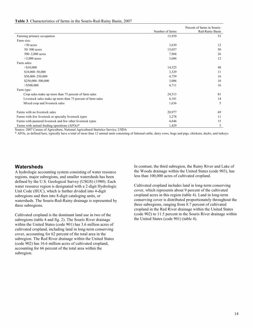
Table 3. Characteristics of farms in the Souris-Red-Rainy Basin, 2007

Number of farms

Percent of farms in Souris-Red-Rainy Basin

Farming primary occupation 15,939 53 Farm size:

<50 acres 3,639 12 50–500 acres 15,037 50 500–2,000 acres 7,968 26 >2,000 acres 3,686 12

Farm sales: <$10,000 14,525 48

$10,000–50,000 3,329 11 $50,000–250,000 4,759 16 $250,000–500,000 3,006 10 >$500,000 4,711 16

Farm type: Crop sales make up more than 75 percent of farm sales 24,513 81

Livestock sales make up more than 75 percent of farm sales 4,181 14 Mixed crop and livestock sales 1,636 5

Farms with no livestock sales 20,977 69 Farms with few livestock or specialty livestock types 3,278 11 Farms with pastured livestock and few other livestock types 4,646 15 Farms with animal feeding operations (AFOs)* 1,429 5

Source: 2007 Census of Agriculture, National Agricultural Statistics Service, USDA * AFOs, as defined here, typically have a total of more than 12 animal units consisting of fattened cattle, dairy cows, hogs and pigs, chickens, ducks, and turkeys. Watersheds A hydrologic accounting system consisting of water resource regions, major subregions, and smaller watersheds has been defined by the U.S. Geological Survey (USGS) (1980). Each water resource region is designated with a 2-digit Hydrologic Unit Code (HUC), which is further divided into 4-digit subregions and then into 8-digit cataloging units, or watersheds. The Souris-Red-Rainy drainage is represented by three subregions. Cultivated cropland is the dominant land use in two of the subregions (table 4 and fig. 2). The Souris River drainage within the United States (code 901) has 3.6 million acres of cultivated cropland, including land in long-term conserving cover, accounting for 62 percent of the total area in the subregion. The Red River drainage within the United States (code 902) has 16.6 million acres of cultivated cropland, accounting for 66 percent of the total area within the subregion.

In contrast, the third subregion, the Rainy River and Lake of the Woods drainage within the United States (code 903), has less than 100,000 acres of cultivated cropland. Cultivated cropland includes land in long-term conserving cover, which represents about 9 percent of the cultivated cropland acres in this region (table 4). Land in long-term conserving cover is distributed proportionately throughout the three subregions, ranging from 8.7 percent of cultivated cropland in the Red River drainage within the United States (code 902) to 11.5 percent in the Souris River drainage within the United States (code 901) (table 4).

14

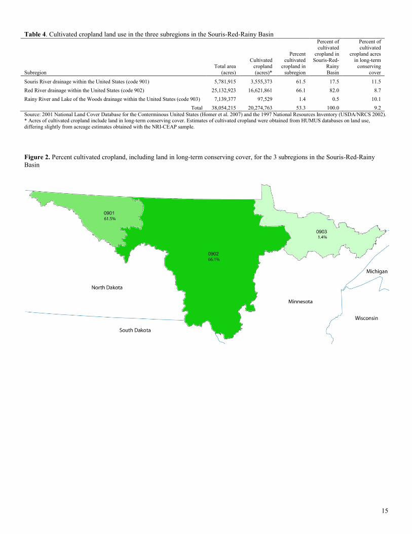
Table 4. Cultivated cropland land use in the three subregions in the Souris-Red-Rainy Basin

Subregion Total area

(acres)

Cultivated cropland (acres)*

Percent cultivated

cropland in subregion

Percent of cultivated

cropland in Souris-Red-

Rainy Basin

Percent of cultivated

cropland acres in long-term

conserving cover

Souris River drainage within the United States (code 901) 5,781,915 3,555,373 61.5 17.5 11.5 Red River drainage within the United States (code 902) 25,132,923 16,621,861 66.1 82.0 8.7 Rainy River and Lake of the Woods drainage within the United States (code 903) 7,139,377 97,529 1.4 0.5 10.1

Total 38,054,215 20,274,763 53.3 100.0 9.2 Source: 2001 National Land Cover Database for the Conterminous United States (Homer et al. 2007) and the 1997 National Resources Inventory (USDA/NRCS 2002). * Acres of cultivated cropland include land in long-term conserving cover. Estimates of cultivated cropland were obtained from HUMUS databases on land use, differing slightly from acreage estimates obtained with the NRI-CEAP sample. Figure 2. Percent cultivated cropland, including land in long-term conserving cover, for the 3 subregions in the Souris-Red-Rainy Basin

15

Chapter 2 Overview of Sampling and Modeling Approach Scope of Study This study was designed to evaluate the effects of conservation practices at the regional scale to provide a better understanding of how conservation practices are benefiting the environment and to determine what challenges remain. The report— • evaluates the extent of conservation practice use in the

region in 2003–06; • estimates the environmental benefits and effects of

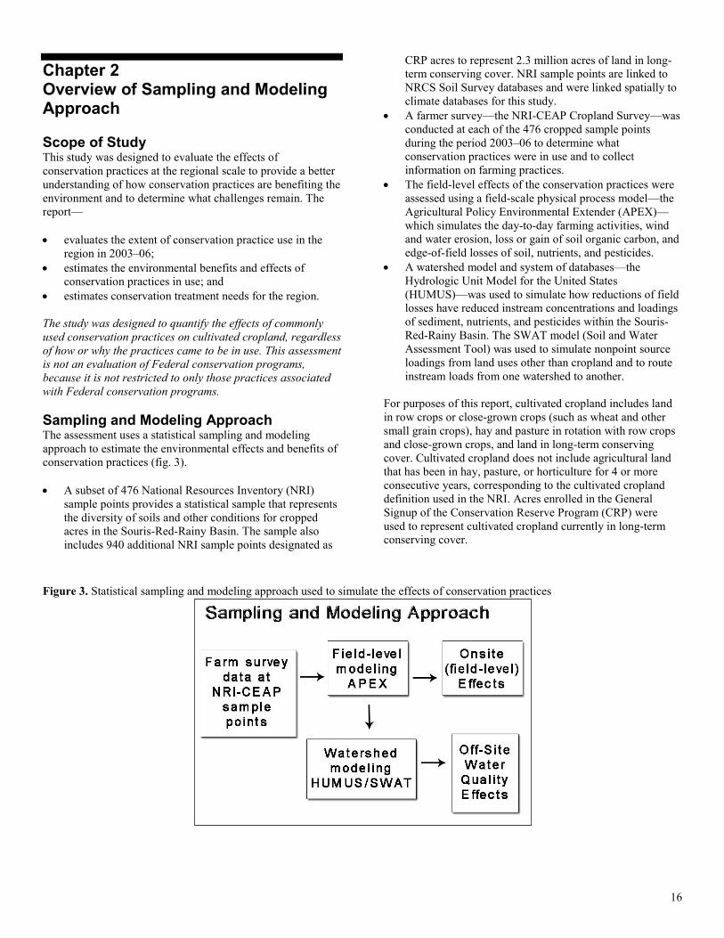
conservation practices in use; and • estimates conservation treatment needs for the region. The study was designed to quantify the effects of commonly used conservation practices on cultivated cropland, regardless of how or why the practices came to be in use. This assessment is not an evaluation of Federal conservation programs, because it is not restricted to only those practices associated with Federal conservation programs. Sampling and Modeling Approach The assessment uses a statistical sampling and modeling approach to estimate the environmental effects and benefits of conservation practices (fig. 3). • A subset of 476 National Resources Inventory (NRI)

sample points provides a statistical sample that represents the diversity of soils and other conditions for cropped acres in the Souris-Red-Rainy Basin. The sample also includes 940 additional NRI sample points designated as

CRP acres to represent 2.3 million acres of land in long-term conserving cover. NRI sample points are linked to NRCS Soil Survey databases and were linked spatially to climate databases for this study.

• A farmer survey—the NRI-CEAP Cropland Survey—was conducted at each of the 476 cropped sample points during the period 2003–06 to determine what conservation practices were in use and to collect information on farming practices.

• The field-level effects of the conservation practices were assessed using a field-scale physical process model—the Agricultural Policy Environmental Extender (APEX)—which simulates the day-to-day farming activities, wind and water erosion, loss or gain of soil organic carbon, and edge-of-field losses of soil, nutrients, and pesticides.

• A watershed model and system of databases—the Hydrologic Unit Model for the United States (HUMUS)—was used to simulate how reductions of field losses have reduced instream concentrations and loadings of sediment, nutrients, and pesticides within the Souris-Red-Rainy Basin. The SWAT model (Soil and Water Assessment Tool) was used to simulate nonpoint source loadings from land uses other than cropland and to route instream loads from one watershed to another.

For purposes of this report, cultivated cropland includes land in row crops or close-grown crops (such as wheat and other small grain crops), hay and pasture in rotation with row crops and close-grown crops, and land in long-term conserving cover. Cultivated cropland does not include agricultural land that has been in hay, pasture, or horticulture for 4 or more consecutive years, corresponding to the cultivated cropland definition used in the NRI. Acres enrolled in the General Signup of the Conservation Reserve Program (CRP) were used to represent cultivated cropland currently in long-term conserving cover.

Figure 3. Statistical sampling and modeling approach used to simulate the effects of conservation practices

16

The modeling strategy for estimating the effects of conservation practices consists of two model scenarios that are produced for each sample point. 1. A baseline scenario, the “baseline conservation condition”

scenario, provides model simulations that account for cropping patterns, farming activities, and conservation practices as reported in the NRI-CEAP Cropland Survey and other sources.

2. An alternative scenario, the “no-practice” scenario, simulates model results as if no conservation practices were in use but holds all other model inputs and parameters the same as in the baseline conservation condition scenario.

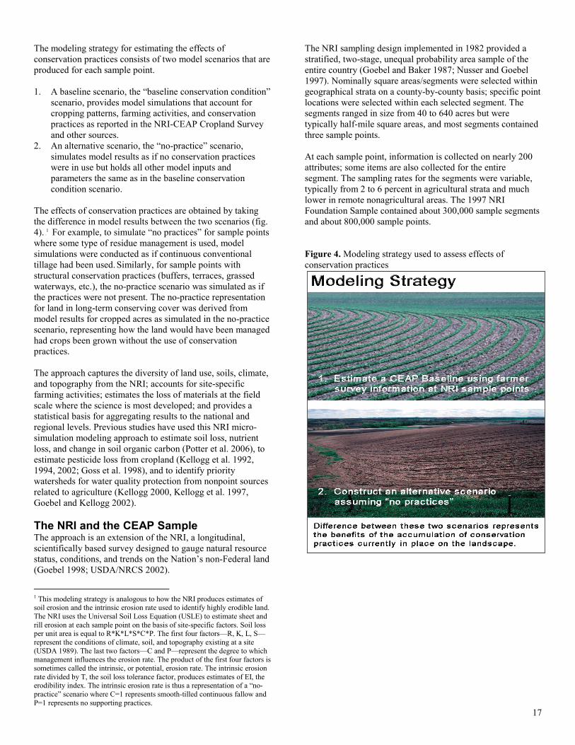
The effects of conservation practices are obtained by taking the difference in model results between the two scenarios (fig. 4).

0F

1 For example, to simulate “no practices” for sample points where some type of residue management is used, model simulations were conducted as if continuous conventional tillage had been used. Similarly, for sample points with structural conservation practices (buffers, terraces, grassed waterways, etc.), the no-practice scenario was simulated as if the practices were not present. The no-practice representation for land in long-term conserving cover was derived from model results for cropped acres as simulated in the no-practice scenario, representing how the land would have been managed had crops been grown without the use of conservation practices. The approach captures the diversity of land use, soils, climate, and topography from the NRI; accounts for site-specific farming activities; estimates the loss of materials at the field scale where the science is most developed; and provides a statistical basis for aggregating results to the national and regional levels. Previous studies have used this NRI micro-simulation modeling approach to estimate soil loss, nutrient loss, and change in soil organic carbon (Potter et al. 2006), to estimate pesticide loss from cropland (Kellogg et al. 1992, 1994, 2002; Goss et al. 1998), and to identify priority watersheds for water quality protection from nonpoint sources related to agriculture (Kellogg 2000, Kellogg et al. 1997, Goebel and Kellogg 2002). The NRI and the CEAP Sample The approach is an extension of the NRI, a longitudinal, scientifically based survey designed to gauge natural resource status, conditions, and trends on the Nation’s non-Federal land (Goebel 1998; USDA/NRCS 2002).

1 This modeling strategy is analogous to how the NRI produces estimates of soil erosion and the intrinsic erosion rate used to identify highly erodible land. The NRI uses the Universal Soil Loss Equation (USLE) to estimate sheet and rill erosion at each sample point on the basis of site-specific factors. Soil loss per unit area is equal to R*K*L*S*C*P. The first four factors—R, K, L, S—represent the conditions of climate, soil, and topography existing at a site (USDA 1989). The last two factors—C and P—represent the degree to which management influences the erosion rate. The product of the first four factors is sometimes called the intrinsic, or potential, erosion rate. The intrinsic erosion rate divided by T, the soil loss tolerance factor, produces estimates of EI, the erodibility index. The intrinsic erosion rate is thus a representation of a “no-practice” scenario where C=1 represents smooth-tilled continuous fallow and P=1 represents no supporting practices.

The NRI sampling design implemented in 1982 provided a stratified, two-stage, unequal probability area sample of the entire country (Goebel and Baker 1987; Nusser and Goebel 1997). Nominally square areas/segments were selected within geographical strata on a county-by-county basis; specific point locations were selected within each selected segment. The segments ranged in size from 40 to 640 acres but were typically half-mile square areas, and most segments contained three sample points. At each sample point, information is collected on nearly 200 attributes; some items are also collected for the entire segment. The sampling rates for the segments were variable, typically from 2 to 6 percent in agricultural strata and much lower in remote nonagricultural areas. The 1997 NRI Foundation Sample contained about 300,000 sample segments and about 800,000 sample points. Figure 4. Modeling strategy used to assess effects of conservation practices

17

NRCS made several significant changes to the NRI program over the past 10 years, including transitioning from a 5-year periodic survey to an annual survey. The NRI’s annual design is a supplemented panel design. 1F

2 A core panel of 41,000 segments is sampled each year, and rotation (supplemental) panels of 31,000 segments each vary by inventory year and allow an inventory to focus on an emerging issue. The core panel and the various supplemental panels are unequal probability subsamples from the 1997 NRI Foundation Sample. The CEAP cultivated cropland sample is a subset of NRI sample points from the 2003 NRI (USDA/NRCS 2007). The 2001, 2002, and 2003 Annual NRI surveys were used to draw the sample.2F

3 The sample is statistically representative of cultivated cropland and formerly cultivated land currently in long-term conserving cover. Nationally, there were over 30,000 samples in the original sample draw. A completed farmer survey was required to include the sample point in the CEAP sample. Some farmers declined to participate in the survey, others could not be located during the time period scheduled for implementing the survey, and other sample points were excluded for administrative reasons such as overlap with other USDA surveys. Some sample points were excluded because the surveys were incomplete or contained inconsistent information, land use found at the sample point had recently changed and was no longer cultivated cropland, or the crops grown were uncommon and model parameters for crop growth were not available. The national NRI-CEAP usable sample consists of about 18,700 NRI points representing cropped acres, and about 13,000 NRI points representing land enrolled in the General Signup of the CRP. The NRI-CEAP Cropland Survey A farmer survey—the NRI-CEAP Cropland Survey—was conducted to obtain the additional information needed for modeling the 476 sample points with crops.3F

4 The USDA National Agricultural Statistics Service (NASS) administered the survey. Farmer participation was voluntary, and the information gathered is confidential. The survey content was specifically designed to provide information on farming activities for use with a physical process model to estimate field-level effects of conservation practices. The survey obtained information on— • crops grown for the previous 3 years, including double

crops and cover crops; • field characteristics, such as proximity to a water body or

wetland and presence of tile or surface drainage systems; • conservation practices associated with the field; • crop rotation plan;

2 For more information on the NRI sample design, see www.nrcs.usda.gov/technical/NRI/. 3 Information about the CEAP sample design is in the documentation report “NRI-CEAP Cropland Survey Design and Statistical Documentation;” see page 5. 4 The surveys, enumerator instructions, and other documentation can be found at http://www.nrcs.usda.gov/wps/portal/nrcs/main/national/technical/nra/ceap/pub/.

• application of commercial fertilizers (rate, timing, method, and form) for crops grown the previous 3 years;

• application of manure (source and type, consistency, application rate, method, and timing) on the field over the previous 3 years;

• application of pesticides (chemical, rate, timing, and method) for the previous 3 years;

• pest management practices; • irrigation practices (system type, amount, and frequency); • timing and equipment used for all field operations (tillage,

planting, cultivation, harvesting) over the previous 3 years; and,

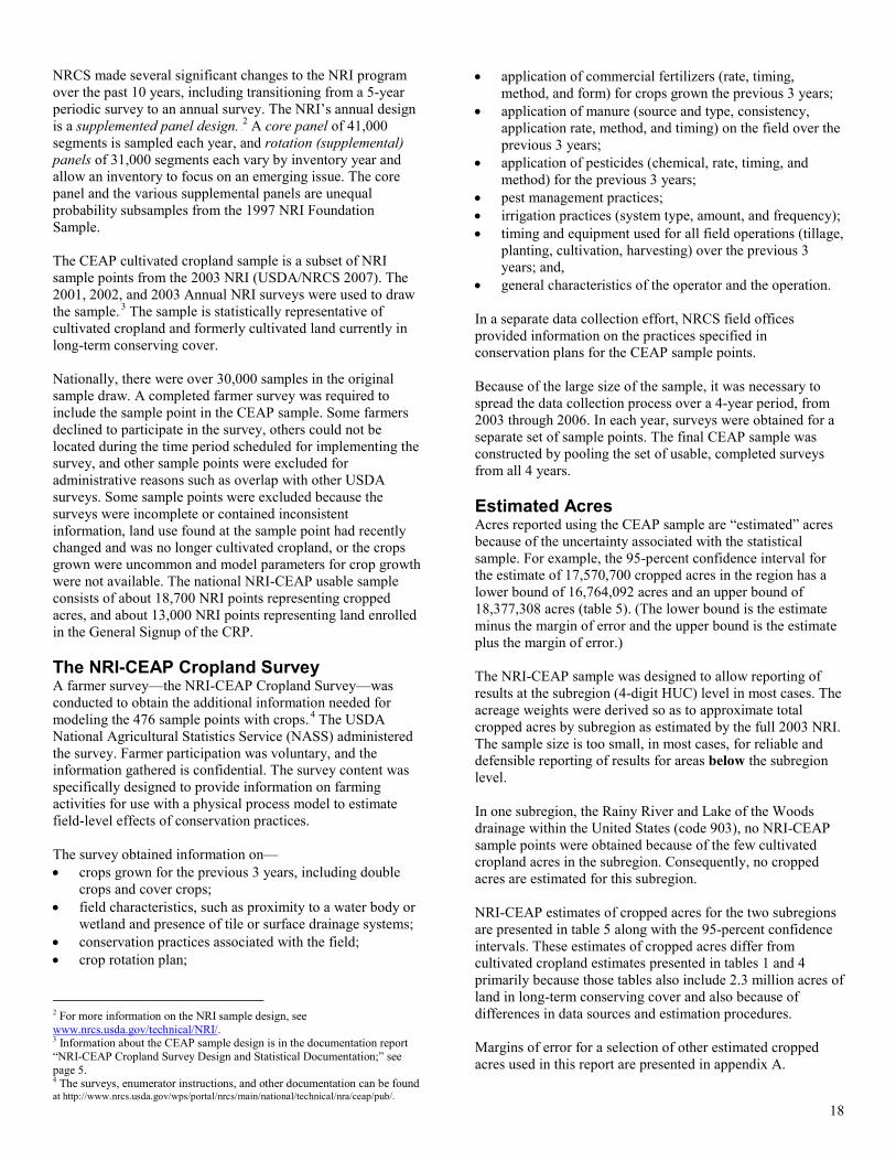
• general characteristics of the operator and the operation. In a separate data collection effort, NRCS field offices provided information on the practices specified in conservation plans for the CEAP sample points. Because of the large size of the sample, it was necessary to spread the data collection process over a 4-year period, from 2003 through 2006. In each year, surveys were obtained for a separate set of sample points. The final CEAP sample was constructed by pooling the set of usable, completed surveys from all 4 years. Estimated Acres Acres reported using the CEAP sample are “estimated” acres because of the uncertainty associated with the statistical sample. For example, the 95-percent confidence interval for the estimate of 17,570,700 cropped acres in the region has a lower bound of 16,764,092 acres and an upper bound of 18,377,308 acres (table 5). (The lower bound is the estimate minus the margin of error and the upper bound is the estimate plus the margin of error.) The NRI-CEAP sample was designed to allow reporting of results at the subregion (4-digit HUC) level in most cases. The acreage weights were derived so as to approximate total cropped acres by subregion as estimated by the full 2003 NRI. The sample size is too small, in most cases, for reliable and defensible reporting of results for areas below the subregion level. In one subregion, the Rainy River and Lake of the Woods drainage within the United States (code 903), no NRI-CEAP sample points were obtained because of the few cultivated cropland acres in the subregion. Consequently, no cropped acres are estimated for this subregion. NRI-CEAP estimates of cropped acres for the two subregions are presented in table 5 along with the 95-percent confidence intervals. These estimates of cropped acres differ from cultivated cropland estimates presented in tables 1 and 4 primarily because those tables also include 2.3 million acres of land in long-term conserving cover and also because of differences in data sources and estimation procedures. Margins of error for a selection of other estimated cropped acres used in this report are presented in appendix A.

18

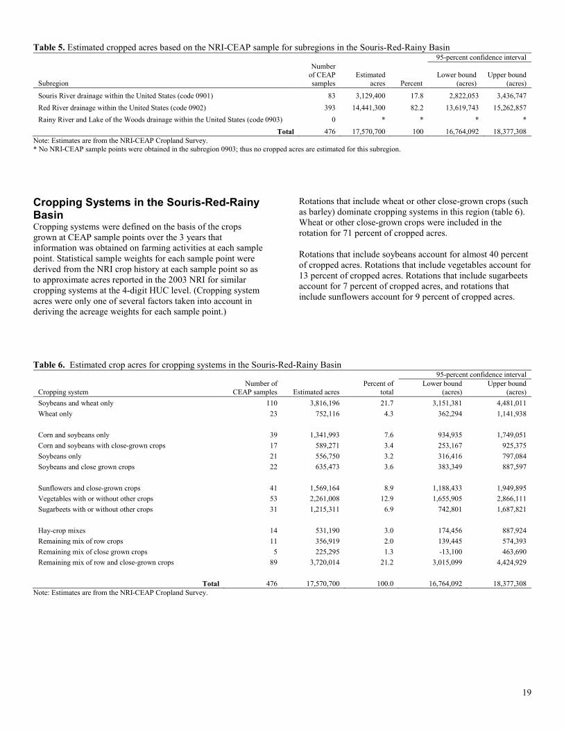
Table 5. Estimated cropped acres based on the NRI-CEAP sample for subregions in the Souris-Red-Rainy Basin

95-percent confidence interval

Subregion

Number of CEAP samples

Estimated acres Percent

Lower bound

(acres)

Upper bound

(acres)

Souris River drainage within the United States (code 0901) 83 3,129,400 17.8 2,822,053 3,436,747 Red River drainage within the United States (code 0902) 393 14,441,300 82.2 13,619,743 15,262,857 Rainy River and Lake of the Woods drainage within the United States (code 0903) 0 * * * *

Total 476 17,570,700 100 16,764,092 18,377,308 Note: Estimates are from the NRI-CEAP Cropland Survey. * No NRI-CEAP sample points were obtained in the subregion 0903; thus no cropped acres are estimated for this subregion. Cropping Systems in the Souris-Red-Rainy Basin Cropping systems were defined on the basis of the crops grown at CEAP sample points over the 3 years that information was obtained on farming activities at each sample point. Statistical sample weights for each sample point were derived from the NRI crop history at each sample point so as to approximate acres reported in the 2003 NRI for similar cropping systems at the 4-digit HUC level. (Cropping system acres were only one of several factors taken into account in deriving the acreage weights for each sample point.)

Rotations that include wheat or other close-grown crops (such as barley) dominate cropping systems in this region (table 6). Wheat or other close-grown crops were included in the rotation for 71 percent of cropped acres. Rotations that include soybeans account for almost 40 percent of cropped acres. Rotations that include vegetables account for 13 percent of cropped acres. Rotations that include sugarbeets account for 7 percent of cropped acres, and rotations that include sunflowers account for 9 percent of cropped acres.

Table 6. Estimated crop acres for cropping systems in the Souris-Red-Rainy Basin

95-percent confidence interval

Cropping system Number of

CEAP samples Estimated acres Percent of

total Lower bound

(acres) Upper bound

(acres) Soybeans and wheat only 110 3,816,196 21.7 3,151,381 4,481,011 Wheat only 23 752,116 4.3 362,294 1,141,938 Corn and soybeans only 39 1,341,993 7.6 934,935 1,749,051 Corn and soybeans with close-grown crops 17 589,271 3.4 253,167 925,375 Soybeans only 21 556,750 3.2 316,416 797,084 Soybeans and close grown crops 22 635,473 3.6 383,349 887,597 Sunflowers and close-grown crops 41 1,569,164 8.9 1,188,433 1,949,895 Vegetables with or without other crops 53 2,261,008 12.9 1,655,905 2,866,111 Sugarbeets with or without other crops 31 1,215,311 6.9 742,801 1,687,821 Hay-crop mixes 14 531,190 3.0 174,456 887,924 Remaining mix of row crops 11 356,919 2.0 139,445 574,393 Remaining mix of close grown crops 5 225,295 1.3 -13,100 463,690 Remaining mix of row and close-grown crops 89 3,720,014 21.2 3,015,099 4,424,929

Total 476 17,570,700 100.0 16,764,092 18,377,308 Note: Estimates are from the NRI-CEAP Cropland Survey.

19

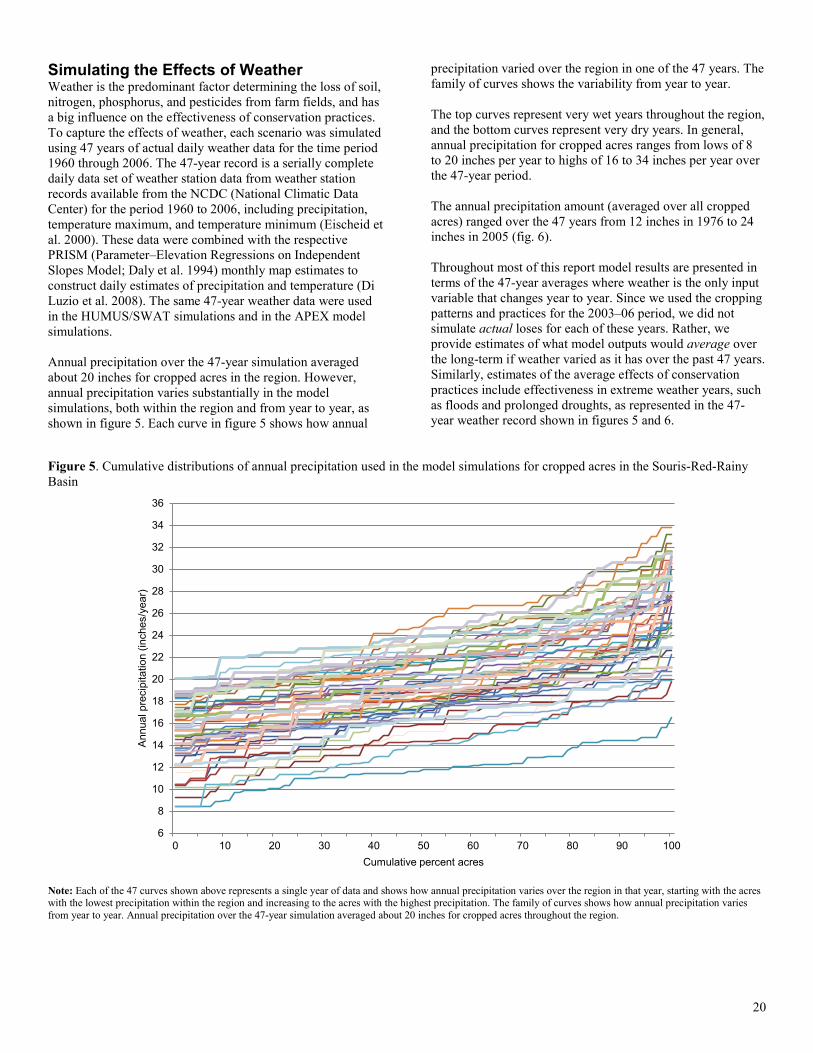
Simulating the Effects of Weather Weather is the predominant factor determining the loss of soil, nitrogen, phosphorus, and pesticides from farm fields, and has a big influence on the effectiveness of conservation practices. To capture the effects of weather, each scenario was simulated using 47 years of actual daily weather data for the time period 1960 through 2006. The 47-year record is a serially complete daily data set of weather station data from weather station records available from the NCDC (National Climatic Data Center) for the period 1960 to 2006, including precipitation, temperature maximum, and temperature minimum (Eischeid et al. 2000). These data were combined with the respective PRISM (Parameter–Elevation Regressions on Independent Slopes Model; Daly et al. 1994) monthly map estimates to construct daily estimates of precipitation and temperature (Di Luzio et al. 2008). The same 47-year weather data were used in the HUMUS/SWAT simulations and in the APEX model simulations. Annual precipitation over the 47-year simulation averaged about 20 inches for cropped acres in the region. However, annual precipitation varies substantially in the model simulations, both within the region and from year to year, as shown in figure 5. Each curve in figure 5 shows how annual

precipitation varied over the region in one of the 47 years. The family of curves shows the variability from year to year. The top curves represent very wet years throughout the region, and the bottom curves represent very dry years. In general, annual precipitation for cropped acres ranges from lows of 8 to 20 inches per year to highs of 16 to 34 inches per year over the 47-year period. The annual precipitation amount (averaged over all cropped acres) ranged over the 47 years from 12 inches in 1976 to 24 inches in 2005 (fig. 6). Throughout most of this report model results are presented in terms of the 47-year averages where weather is the only input variable that changes year to year. Since we used the cropping patterns and practices for the 2003–06 period, we did not simulate actual loses for each of these years. Rather, we provide estimates of what model outputs would average over the long-term if weather varied as it has over the past 47 years. Similarly, estimates of the average effects of conservation practices include effectiveness in extreme weather years, such as floods and prolonged droughts, as represented in the 47-year weather record shown in figures 5 and 6.

Figure 5. Cumulative distributions of annual precipitation used in the model simulations for cropped acres in the Souris-Red-Rainy Basin

Note: Each of the 47 curves shown above represents a single year of data and shows how annual precipitation varies over the region in that year, starting with the acres with the lowest precipitation within the region and increasing to the acres with the highest precipitation. The family of curves shows how annual precipitation varies from year to year. Annual precipitation over the 47-year simulation averaged about 20 inches for cropped acres throughout the region.

6

8

10

12

14

16

18

20

22

24

26

28

30

32

34

36

0 10 20 30 40 50 60 70 80 90 100

Ann

ual p

reci

pita

tion

(inch

es/y

ear)

Cumulative percent acres

20

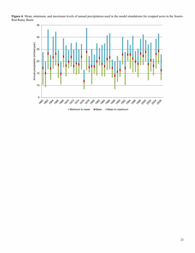
Figure 6. Mean, minimum, and maximum levels of annual precipitation used in the model simulations for cropped acres in the Souris-Red-Rainy Basin

5

10

15

20

25

30

35

Ann

ual p

reci

pita

tion

(inch

es/y

ear)

Minimum to mean Mean Mean to maximum

21

Chapter 3 Evaluation of Conservation Practice Use—the Baseline Conservation Condition This study assesses the use and effectiveness of conservation practices in the Souris-Red-Rainy Basin for the period 2003 to 2006 to determine the baseline conservation condition for the region. The baseline conservation condition provides a benchmark for estimating the effects of existing conservation practices as well as projecting the likely effects of alternative conservation treatment. Conservation practices that were evaluated include structural practices, annual practices, and long-term conserving cover. Structural conservation practices, once implemented, are usually kept in place for several years. Designed primarily for erosion control, they also mitigate edge-of-field nutrient and pesticide loss. Structural practices evaluated include— • in-field practices for water erosion control, divided into

two groups: o practices that control overland flow (terraces, contour

buffer strips, contour farming, stripcropping, contour stripcropping), and

o practices that control concentrated flow (grassed waterways, grade stabilization structures, diversions, and other structures for water control);

• edge-of-field practices for buffering and filtering surface runoff before it leaves the field (riparian forest buffers, riparian herbaceous cover, filter strips, field borders); and

• wind erosion control practices (windbreaks/shelterbelts, cross wind trap strips, herbaceous wind barriers, hedgerow planting).

Annual conservation practices are management practices conducted as part of the crop production system each year. These practices are designed primarily to promote soil quality, reduce in-field erosion, and reduce the availability of sediment, nutrients, and pesticides for transport by wind or water. They include— • residue and tillage management; • nutrient management practices; • irrigation water management; • pesticide management practices; and • cover crops.

Long-term conservation cover establishment consists of planting suitable native or domestic grasses, forbs, or trees on environmentally sensitive cultivated cropland. Historical Context for Conservation Practice Use The use of conservation practices in the Souris-Red-Rainy Basin closely reflects the history of Federal conservation programs and technical assistance. In the beginning the focus was almost entirely on reducing soil erosion and preserving the soil’s productive capacity. In the 1930s and 1940s, Hugh

Hammond Bennett, the founder and first chief of the Soil Conservation Service (now Natural Resources Conservation Service) instilled in the national ethic the need to treat every acre to its potential by controlling soil erosion and water runoff. Land shaping structural practices (such as terraces, contour farming, and stripcropping) and sediment control structures were widely adopted where appropriate. Conservation tillage emerged in the 1970s as a key management practice for enhancing soil quality and further reducing soil erosion. Conservation tillage, along with use of crop rotations and cover crops, was used either alone or in combination with structural practices. The conservation compliance provisions in the 1985 Farm Bill sharpened the focus to treatment of the most erodible acres, tying farm commodity payments to conservation treatment of highly erodible land. The Conservation Reserve Program was established to enroll the most erodible cropland acres in multi-year contracts to plant acres in long-term conserving cover. During the 1990s, the focus of conservation efforts began to shift from soil conservation and sustainability to reducing pollution impacts associated with agricultural production. Prominent among new concerns were the environmental effects of nutrient export from farm fields. Traditional conservation practices used to control surface water runoff and erosion control were mitigating a significant portion of these nutrient losses. Additional gains were being achieved using nutrient management practices—application of nutrients (appropriate timing, rate, method, and form) to minimize losses to the environment and maximize the availability of nutrients for crop growth. Summary of Practice Use The conservation practice information collected during the study was used to assess the extent of conservation practice use in the Souris-Red-Rainy Basin. Key findings are the following: • Structural practices for controlling water erosion are in

use on 18 percent of cropped acres. On the 13 percent of the acres designated as highly erodible land, structural practices designed to control water erosion are in use on 23 percent.

• Structural practices for controlling wind erosion are in use on 20 percent of cropped acres. On the 13 percent of the acres designated as highly erodible land, structural practices designed to control wind erosion are in use on 26 percent.

• Reduced tillage is common in the region; 72 percent of the cropped acres meet criteria for either no-till (17 percent) or mulch till (55 percent). All but 12 percent of the acres had evidence of some kind of reduced tillage on at least one crop.

• About 37 percent of cropped acres are gaining soil organic carbon.

• Producers use either residue and tillage management practices or structural practices, or both, on 89 percent of cropped acres.

• The use of nutrient management practices is more widespread in this region than in other regions.

22

o About 1 percent of cropped acres have no nitrogen

applied. An additional 64 percent of cropped acres meet criteria for timing of nitrogen applications on all crops in the rotation, 78 percent meet criteria for method of application, and 71 percent meet criteria for rate of application.

o About 2 percent of cropped acres have no phosphorus applied. An additional 79 percent of cropped acres meet criteria for timing of phosphorus applications on all crops in the rotation, 83 percent meet criteria for method of application, and 55 percent meet criteria for rate of application.

o Appropriate nitrogen application rates, timing of application, and application method for all crops during every year of production are in use on 38 percent of cropped acres.

o Good phosphorus management practices (appropriate rate, timing, and method) are in use on 43 percent of the acres on all crops during every year of production.

o About 25 percent of cropped acres meet nutrient management criteria for both nitrogen and phosphorus management, including acres with no nutrient applications.

• During the 2003–06 period of data collection, criteria for cover crops were not met on any CEAP sample points in this region.

• The Integrated Pest Management (IPM) indicator showed that about 19 percent of the acres were being managed with a relatively high level of IPM.

• Land in long-term conserving cover, as represented by enrollment in the CRP General Signup, consists of 2.3 million acres in the region, of which 29 percent is highly erodible land.

Structural Conservation Practices Data on structural practices for the farm field associated with each sample point were obtained from four sources: 1. The NRI-CEAP Cropland Survey included questions

about the presence of 12 types of structural practices: terraces, grassed waterways, vegetative buffers (in-field), hedgerow plantings, riparian forest buffers, riparian herbaceous buffers, windbreaks or herbaceous wind barriers, contour buffers (in-field), field borders, filter strips, critical area planting, and grade stabilization structures.

2. For fields with conservation plans, NRCS field offices provided data on all structural practices included in the plans.

3. The USDA-Farm Service Agency (FSA) provided practice information for fields that were enrolled in the Continuous CRP for these structural practices: contour grass strips, filter strips, grassed waterways, riparian buffers (trees), and field windbreaks (Alex Barbarika, USDA/FSA, personal communication).

4. The 2003 NRI provided additional information for practices that could be reliably identified from aerial photography as part of the NRI data collection process. These practices include contour buffer strips, contour

farming, contour stripcropping, field stripcropping, terraces, cross wind stripcropping, cross wind trap strips, diversions, field borders, filter strips, grassed waterways or outlets, hedgerow planting, herbaceous wind barriers, riparian forest buffers, and windbreak or shelterbelt establishment.

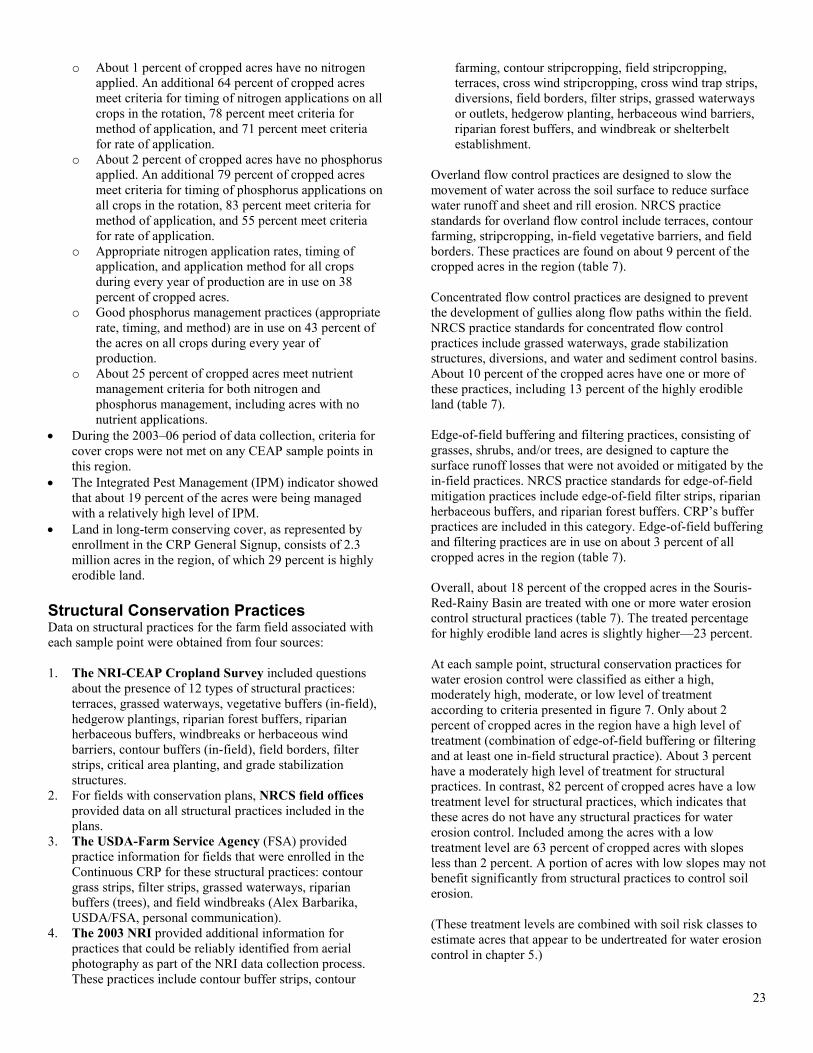
Overland flow control practices are designed to slow the movement of water across the soil surface to reduce surface water runoff and sheet and rill erosion. NRCS practice standards for overland flow control include terraces, contour farming, stripcropping, in-field vegetative barriers, and field borders. These practices are found on about 9 percent of the cropped acres in the region (table 7). Concentrated flow control practices are designed to prevent the development of gullies along flow paths within the field. NRCS practice standards for concentrated flow control practices include grassed waterways, grade stabilization structures, diversions, and water and sediment control basins. About 10 percent of the cropped acres have one or more of these practices, including 13 percent of the highly erodible land (table 7). Edge-of-field buffering and filtering practices, consisting of grasses, shrubs, and/or trees, are designed to capture the surface runoff losses that were not avoided or mitigated by the in-field practices. NRCS practice standards for edge-of-field mitigation practices include edge-of-field filter strips, riparian herbaceous buffers, and riparian forest buffers. CRP’s buffer practices are included in this category. Edge-of-field buffering and filtering practices are in use on about 3 percent of all cropped acres in the region (table 7). Overall, about 18 percent of the cropped acres in the Souris-Red-Rainy Basin are treated with one or more water erosion control structural practices (table 7). The treated percentage for highly erodible land acres is slightly higher—23 percent. At each sample point, structural conservation practices for water erosion control were classified as either a high, moderately high, moderate, or low level of treatment according to criteria presented in figure 7. Only about 2 percent of cropped acres in the region have a high level of treatment (combination of edge-of-field buffering or filtering and at least one in-field structural practice). About 3 percent have a moderately high level of treatment for structural practices. In contrast, 82 percent of cropped acres have a low treatment level for structural practices, which indicates that these acres do not have any structural practices for water erosion control. Included among the acres with a low treatment level are 63 percent of cropped acres with slopes less than 2 percent. A portion of acres with low slopes may not benefit significantly from structural practices to control soil erosion. (These treatment levels are combined with soil risk classes to estimate acres that appear to be undertreated for water erosion control in chapter 5.)

23

Table 7. Structural conservation practices in use for the baseline conservation condition, Souris-Red-Rainy Basin

Structural practice category Conservation practice in use

Percent of non-

HEL Percent of HEL

Percent of

cropped acres

Overland flow control practices Terraces, contour buffer strips, contour farming, stripcropping, contour

stripcropping, field border, in-field vegetative barriers 9 10 9

Concentrated flow control practices Grassed waterways, grade stabilization structures, diversions, other structures

for water control 9 13 10

Edge-of-field buffering and filtering practices Riparian forest buffers, riparian herbaceous buffers, filter strips 4 0 3

One or more water erosion control practices Overland flow, concentrated flow, or edge-of-field practice 18 23 18

Wind erosion control practices

Windbreaks/shelterbelts, cross wind trap strips, herbaceous windbreak, hedgerow planting 19 26 20

Note: About 13 percent of cropped acres in the Souris-Red-Rainy Basin are highly erodible land (HEL). Soils are classified as HEL if they have an erodibility index (EI) score of 8 or higher. A numerical expression of the potential of a soil to erode, EI considers the physical and chemical properties of the soil and climatic conditions where it is located. The higher the index, the greater the investment needed to maintain the sustainability of the soil resource base if intensively cropped. Figure 7. Percent of cropped acres at four conservation treatment levels for structural practices, baseline conservation condition, Souris-Red-Rainy Basin

Criteria for four levels of treatment with structural conservation practices are: • High treatment: Edge-of-field mitigation and at least one in-field structural practice (concentrated flow or overland flow practice) required. • Moderately high treatment: Either edge-of-field mitigation required or both concentrated flow and overland flow practices required. • Moderate treatment: No edge-of-field mitigation, either concentrated flow or overland flow practices required. • Low treatment: No edge-of-field or in-field structural practices. Note: See appendix B, table B3, for a breakdown of conservation treatment levels by subregion.

Low Moderate Moderatelyhigh High

Slope 2 percent or less 63.3 9.2 2.0 1.7Slope greater than 2 percent 18.4 4.4 0.7 0.2

81.7

13.6

2.8 1.9

0

10

20

30

40

50

60

70

80

90

Perc

ent o

f cro

pped

acr

es

24

Wind erosion control practices are designed to reduce the force of the wind on the field. NRCS structural practice standards for wind erosion control practices include cross wind ridges, cross wind trap strips, herbaceous wind barriers, and windbreak/shelterbelt establishment. Wind erosion is a resource concern for many cropped acres in this region. About 20 percent of the cropped acres in the region are treated for wind erosion using structural practices (table 7). Residue and Tillage Management Practices Simulations of the use of residue and tillage management practices were based on the field operations and machinery types reported in the NRI-CEAP Cropland Survey for each sample point. The survey obtained information on the timing, type, and frequency of each tillage implement used during the previous 3 years, including the crop to which the tillage operation applied. Model outcomes affected by tillage practices, such as erosion and runoff, were determined based on APEX processes of the daily tillage activities as reported in the survey. To evaluate the level of residue and tillage management, the Soil Tillage Intensity Rating (STIR) (USDA/NRCS 2007) was used for tillage intensity and gains or losses in soil organic carbon (based on model simulation results) were used as an indicator of residue management. STIR values represent the soil disturbance intensity, which was estimated for each crop at each sample point.4F

5 The soil disturbance intensity is a function of the kinds of tillage, the frequency of tillage, and the depth of tillage. STIR values were calculated for each crop and for each of the 3 years covered by the NRI-CEAP Cropland Survey (accounting for multiple crops or cover crops). By combining the STIR values for each crop year with model output on the long-term trend in soil organic carbon gain or loss, eight categories of residue and tillage management were identified.5F

6 Overall, 72 percent of cropped acres in the Souris-Red-Rainy Basin meet the tillage intensity rating for either no-till or mulch till (table 8). About 17 percent meet the criteria for no-till, and 55 percent meet the tillage intensity criteria for mulch till. About 17 percent of cropped acres do not meet criteria for mulch till or no-till but have reduced tillage on some crops in the rotation. Only 12 percent of the acres are conventionally tilled for all crops in the rotation. To evaluate the use of residue and tillage management practices, practice use was classified as high, moderately high, moderate, or low for each sample point according to criteria presented in figure 8. (These residue and tillage management treatment levels were combined with the use of structural

5 Percent residue cover was not used to evaluate no-till or mulch till because this criterion is not included in the current NRCS practice standard for Residue and Tillage Management. Residue is, however, factored into erosion and runoff estimates in APEX. 6 STIR values in combination with carbon trends are in line with the use of the Soil Conditioning Index (SCI), which approximates the primary criteria for NRCS residue management standards. The NRCS practice standard, as applied at the field, may include other considerations to meet site specific resource concerns that are not considered in this evaluation.

practices to estimate conservation treatment levels for water erosion control in chapter 5.) The high and moderately high treatment levels represent the 33 percent of cropped acres that meet tillage intensity criteria for either no-till or mulch till and are gaining soil organic carbon. The high treatment level, representing 28 percent of cropped acres, includes only those acres with gains in soil organic carbon and where the tillage intensity criteria are met for each crop in the rotation. About 5 percent of cropped acres have a moderately high treatment level, where the average annual tillage intensity meets criteria for mulch till or no-till and the crop rotation is gaining soil organic carbon. The majority of the cropped acres—58 percent—have a moderate level of treatment. Most of these acres meet tillage intensity for no-till or mulch till but are losing soil organic carbon. Other acres have reduced tillage but do not meet criteria for no-till or mulch till, or they are gaining soil organic carbon but tillage intensity exceeds criteria for mulch till (fig. 8). About 10 percent of the acres have a low treatment level, consisting of continuous conventional tillage for all crops in the rotation and loss of soil organic carbon. Structural practices and residue and tillage management practices influence losses of sediment, nutrients, and pesticides due to water erosion. Most of the cropped acres (89 percent) in the Souris-Red-Rainy Basin have one or both of these types of water erosion control practices (table 9). About 14 percent meet tillage intensity for no-till or mulch till and have structural practices, including 17 percent of HEL. About 57 percent of cropped acres meet tillage criteria for no-till or mulch till without structural practices in use. Only 1 percent have structural practices without any kind of residue or tillage management (table 9). Conservation Crop Rotation In the Souris-Red-Rainy Basin, nearly all crop rotations meet NRCS criteria for conservation crop rotations (NRCS practice code 328). This practice consists of growing different crops in a planned rotation to manage nutrient and pesticide inputs, enhance soil quality, or reduce soil erosion. Including a legume, hay, or close grown crop in the rotation can have a pronounced effect on long-term average field losses of sediment and nutrients, as well as enhancement of soil quality. In the Souris-Red-Rainy Basin, only 15 percent of cropped acres are in continuous row cropping. The model outputs reported in chapter 4 reflect the effects of conservation crop rotations, but the benefits of conservation crop rotation practices could not be assessed quantitatively in this study. First, it was not possible to differentiate conservation crop rotations from crop rotations for other purposes, such as the control of pests or in response to changing markets. Second, the “no-practice scenario” would require simulation of mono-cropping systems, which would require arbitrary decisions about which crops to simulate at each sample point to preserve the level of regional production.

25

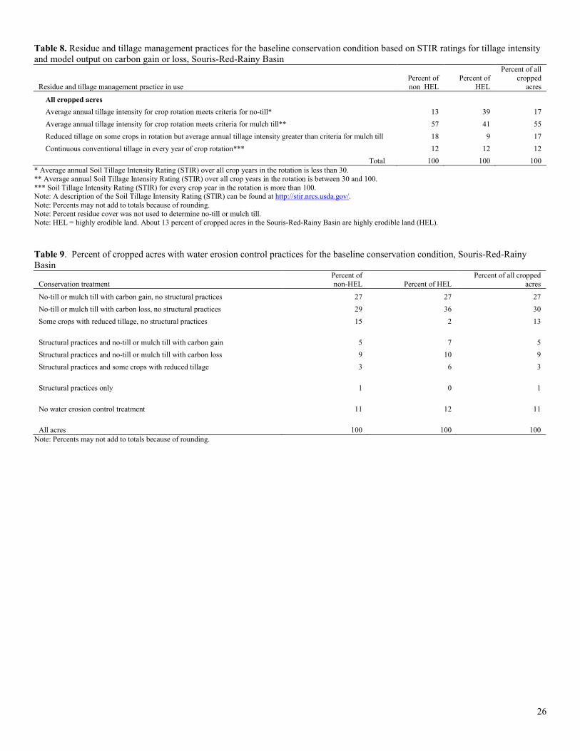
Table 8. Residue and tillage management practices for the baseline conservation condition based on STIR ratings for tillage intensity and model output on carbon gain or loss, Souris-Red-Rainy Basin

Residue and tillage management practice in use Percent of non_HEL

Percent of HEL

Percent of all cropped

acres

All cropped acres Average annual tillage intensity for crop rotation meets criteria for no-till* 13 39 17

Average annual tillage intensity for crop rotation meets criteria for mulch till** 57 41 55 Reduced tillage on some crops in rotation but average annual tillage intensity greater than criteria for mulch till 18 9 17 Continuous conventional tillage in every year of crop rotation*** 12 12 12

Total 100 100 100 * Average annual Soil Tillage Intensity Rating (STIR) over all crop years in the rotation is less than 30. ** Average annual Soil Tillage Intensity Rating (STIR) over all crop years in the rotation is between 30 and 100. *** Soil Tillage Intensity Rating (STIR) for every crop year in the rotation is more than 100. Note: A description of the Soil Tillage Intensity Rating (STIR) can be found at http://stir.nrcs.usda.gov/. Note: Percents may not add to totals because of rounding. Note: Percent residue cover was not used to determine no-till or mulch till. Note: HEL = highly erodible land. About 13 percent of cropped acres in the Souris-Red-Rainy Basin are highly erodible land (HEL). Table 9. Percent of cropped acres with water erosion control practices for the baseline conservation condition, Souris-Red-Rainy Basin

Conservation treatment Percent of non-HEL Percent of HEL

Percent of all cropped acres

No-till or mulch till with carbon gain, no structural practices 27 27 27 No-till or mulch till with carbon loss, no structural practices 29 36 30 Some crops with reduced tillage, no structural practices 15 2 13 Structural practices and no-till or mulch till with carbon gain 5 7 5 Structural practices and no-till or mulch till with carbon loss 9 10 9 Structural practices and some crops with reduced tillage 3 6 3 Structural practices only 1 0 1 No water erosion control treatment 11 12 11 All acres 100 100 100

Note: Percents may not add to totals because of rounding.

26

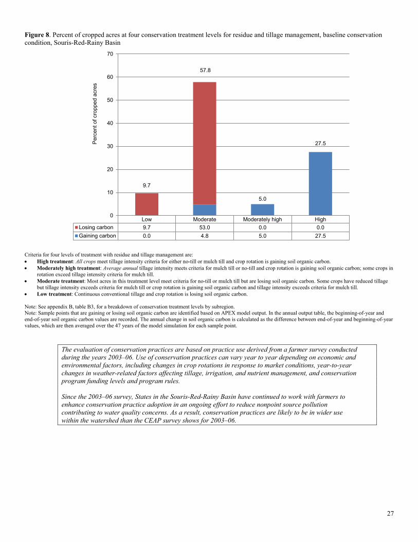
Figure 8. Percent of cropped acres at four conservation treatment levels for residue and tillage management, baseline conservation condition, Souris-Red-Rainy Basin

Criteria for four levels of treatment with residue and tillage management are: • High treatment: All crops meet tillage intensity criteria for either no-till or mulch till and crop rotation is gaining soil organic carbon. • Moderately high treatment: Average annual tillage intensity meets criteria for mulch till or no-till and crop rotation is gaining soil organic carbon; some crops in

rotation exceed tillage intensity criteria for mulch till. • Moderate treatment: Most acres in this treatment level meet criteria for no-till or mulch till but are losing soil organic carbon. Some crops have reduced tillage

but tillage intensity exceeds criteria for mulch till or crop rotation is gaining soil organic carbon and tillage intensity exceeds criteria for mulch till. • Low treatment: Continuous conventional tillage and crop rotation is losing soil organic carbon. Note: See appendix B, table B3, for a breakdown of conservation treatment levels by subregion. Note: Sample points that are gaining or losing soil organic carbon are identified based on APEX model output. In the annual output table, the beginning-of-year and end-of-year soil organic carbon values are recorded. The annual change in soil organic carbon is calculated as the difference between end-of-year and beginning-of-year values, which are then averaged over the 47 years of the model simulation for each sample point.

The evaluation of conservation practices are based on practice use derived from a farmer survey conducted during the years 2003–06. Use of conservation practices can vary year to year depending on economic and environmental factors, including changes in crop rotations in response to market conditions, year-to-year changes in weather-related factors affecting tillage, irrigation, and nutrient management, and conservation program funding levels and program rules. Since the 2003–06 survey, States in the Souris-Red-Rainy Basin have continued to work with farmers to enhance conservation practice adoption in an ongoing effort to reduce nonpoint source pollution contributing to water quality concerns. As a result, conservation practices are likely to be in wider use within the watershed than the CEAP survey shows for 2003–06.

Low Moderate Moderately high HighLosing carbon 9.7 53.0 0.0 0.0Gaining carbon 0.0 4.8 5.0 27.5

9.7

57.8

5.0

27.5

0

10

20

30

40

50

60

70

Per

cent

of c

ropp

ed a

cres

27

Cover Crops Cover crops are planted when the principal crops are not growing. The two most important functions of cover crops from a water quality perspective are (1) to provide soil surface cover and reduce soil erosion, and (2) to utilize and convert excess nutrients remaining in the soil from the preceding crop into plant biomass, thereby reducing nutrient leaching and minimizing the amount of soluble nutrients in runoff during the non-crop growing season. From a soil quality perspective, cover crops help capture atmospheric carbon in plant tissue, provide habitat for the soil food web, and stabilize or enhance soil aggregate strength. The presence or absence of cover crops was determined from farmer responses in the NRI-CEAP Cropland Survey. The following criteria were used to identify a cover crop. • A cover crop must be a close-grown crop that is not

harvested as a principal crop, or if it is harvested, must have been specifically identified in the NRI-CEAP Cropland Survey as a cover crop as an indicator that the harvest was for an acceptable purpose (such as biomass removal or use as mulch or forage material).

• Spring-planted cover crops are inter-seeded into a growing crop or are followed by the seeding of a summer or late fall crop that may be harvested during that same year or early the next year.

• Late-summer-planted cover crops are followed by the harvest of another crop in the same crop year or the next spring.

• Fall-planted cover crops are followed by the spring planting of a crop for harvest the next year.

Some cover crops are planted for soil protection during establishment. In the Souris-Red-Rainy Basin, cover crops were rarely used as a conservation practice during the period covered by the farmer survey (2003–06). The above criteria for a cover crop were not met on any CEAP sample points in this region. Irrigation Management Practices Irrigation in the United States has its roots in the arid West where precipitation is insufficient to meet the needs of growing crops. In other parts of the United States, rainfall totals are sufficient in most years to produce satisfactory yields. The distribution of the rainfall during the crop growing season, however, is sometimes problematic, especially in years when precipitation is below average. In the Souris-Red-Rainy Basin, irrigation is rarely used. Only two CEAP sample points reported irrigation water applications, representing 88,000 acres. Nutrient Management Practices Nitrogen and phosphorus are essential inputs to profitable crop production. Farmers apply these nutrients to the land as commercial fertilizers and manure to promote plant growth and increase crop yields. Not all of the nutrients applied to the land, however, are taken up by crops; some are lost to the

environment, which can contribute to offsite water quality problems. Sound nutrient management systems can minimize nutrient losses from the agricultural management zone while providing adequate soil fertility and nutrient availability to ensure realistic yields. (The agricultural management zone is defined as the zone surrounding a field that is bounded by the bottom of the root zone, edge of the field, and top of the crop canopy.) Such systems are tailored to address the specific cropping system, nutrient sources available, and site characteristics of each field. Nutrient management systems have four basic criteria for application of commercial fertilizers and manure. 6F

7 1. Apply nutrients at the appropriate rate based on soil and

plant tissue analyses and realistic yield goals. 2. Apply the appropriate form of fertilizer and organic

material with compositions and characteristics that resist nutrient losses from the agricultural management zone.

3. Apply at the appropriate time to supply nutrients to the crop when the plants have the most active uptake and biomass production, and avoid times when adverse weather conditions can result in large losses of nutrients from the agricultural management zone.

4. Apply using the appropriate application method that provides nutrients to the plants for rapid, efficient uptake and reduces the exposure of nutrient material to forces of wind and water.

Depending on the field characteristics, these nutrient management techniques can be coupled with other conservation practices such as conservation crop rotations, cover crops, residue management practices, and structural practices to minimize the potential for nutrient losses from the agricultural management zone. Even though nutrient transport and losses from agricultural fields cannot be completely eliminated, they can be minimized by careful management and kept within an acceptable level. The presence or absence of nutrient management practices was based on information on the timing, rate, and method of application for manure and commercial fertilizer as reported by the producer in the NRI-CEAP Cropland Survey. The appropriate form of nutrients applied was not evaluated because the survey was not sufficiently specific about the material formulations that were applied. The following criteria were used to identify the appropriate rate, time, and method of nutrient application for each crop or crop rotation. • All commercial fertilizer and manure applications are

within 3 weeks prior to plant date, at planting, or within 60 days after planting. For fall-planted winter wheat, spring applications also were considered appropriate timing.

• The method of application for commercial fertilizer or manure is some form of incorporation or banding or spot treatment or foliar applied.

7 These criteria are also referred to as “4R nutrient stewardship—right source, right rate, right time, and right place” (Bruulsema et al. 2009).

28

• The rate of nitrogen application, including the sum of

both commercial fertilizer and manure nitrogen available for crops in the year of application, is— o less than 1.4 times the amount of nitrogen removed in

the crop yield at harvest for each crop,7F

8 except for small grain crops; or

o less than 1.6 times the amount of nitrogen removed in the crop yield at harvest for small grain crops (wheat, barley, oats, rice, rye, buckwheat, emmer, spelt, and triticale).

• The rate of phosphorus application summed over all applications and crops in the rotation, including both commercial fertilizer and manure phosphorus, is less than 1.1 times the amount of phosphorus removed in the crop yields at harvest summed over all crops in the rotation.

Only about 3 percent of cropped acres in this region had manure applied, according to the CEAP cropland survey for 2003–06. Phosphorus application rate criteria apply to the full crop rotation to account for infrequent applications intended to provide phosphorus for multiple crops or crop years, which is often the case with manure applications. Nitrogen application rate criteria apply to each crop in the rotation. These nutrient management criteria are intended to represent practice recommendations commonly found in comprehensive nutrient management conservation plans and generally are consistent with recommended rates. While consistent with NRCS standards, they do not necessarily represent the best possible set of nutrient management practices. For example, lower application rates are possible when timing and method criteria are also met and when soil erosion and runoff are controlled. As shown in table 10, the majority of acres in the Souris-Red-Rainy Basin meet one or more of the criteria for nitrogen management. About 1 percent of cropped acres have no nitrogen applied. An additional 64 percent of cropped acres meet criteria for timing of nitrogen applications on all crops in the rotation, 78 percent meet criteria for method of application, and 71 percent meet criteria for rate of application. Similar results were found for phosphorus management. About 2 percent of cropped acres have no phosphorus applied. An additional 79 percent of cropped acres meet criteria for timing of phosphorus applications on all crops in the rotation, 83 percent meet criteria for method of application, and 55 percent meet criteria for rate of application. Somewhat fewer acres, however, meet all nutrient management criteria (table 10):

8 The 1.4 ratio of application rate to yield represents 70-percent use efficiency for applied nitrogen, which has traditionally been accepted as good nitrogen management practice. The 30 percent “lost” includes plant biomass left in the field, volatilization during and following application, immobilization by soil and soil microbes, and surface runoff and leaching losses. A slightly higher ratio is used for small grain crops to maintain yields at current levels.

• In addition to the 1 percent of cropped acres without nitrogen applications, 38 percent of the acres meet all criteria for nitrogen applications;

• In addition to the 2 percent of cropped acres without phosphorus applications, 43 percent of the acres meet all criteria for phosphorus applications;

• 25 percent of cropped acres meet criteria for both phosphorus and nitrogen management, including acres with no nutrient applications.

Lower nitrogen rate criteria are appropriate for acres that meet application timing and method criteria and also are fully treated for soil erosion control because more of the nitrogen applied is retained on the field and is therefore available for crop growth. Through additional simulation modeling, the following nitrogen rates were found to be possible when timing and method were good and when appropriate soil erosion control practices were in use:: • 1.2 times the amount of nitrogen removed in the crop

yield at harvest for each crop, except for small grain crops; or

• 1.5 times the amount of nitrogen removed in the crop yield at harvest for small grain crops.

About 23 percent of cropped acres in the region meet all nutrient management criteria including these lower nitrogen rate criteria and including acres not receiving nutrient applications (table 10). Four levels of treatment for nitrogen and phosphorus management were derived for use in evaluating the adequacy of nutrient management. (These treatment levels are combined with soil risk classes to estimate acres that appear to be undertreated in chapter 5.) Criteria for the treatment levels are presented in figures 9 and 10. The high treatment level represents consistent use of appropriate rate, timing, and method for all crops, including the lower nitrogen application rate criteria appropriate for full conservation treatment conditions. Based on these treatment levels, about 37 percent of the acres in the Souris-Red-Rainy Basin have a high level of nitrogen management and about 36 percent have a moderately high level of nitrogen management (fig. 9). About 23 percent of cropped acres have a moderate treatment level for nitrogen and only 4 percent of have a low level of nitrogen management. About 45 percent of cropped acres have a high level of phosphorus management (fig 10). About 12 percent of have a moderately high treatment level and about 25 percent have a moderate treatment level for phosphorus. About 18 percent of cropped acres have a low level of phosphorus management.

29

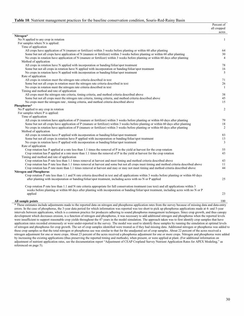
Table 10. Nutrient management practices for the baseline conservation condition, Souris-Red-Rainy Basin Percent of

all cropped acres

Nitrogen* No N applied to any crop in rotation 1 For samples where N is applied:

Time of application All crops have application of N (manure or fertilizer) within 3 weeks before planting or within 60 after planting 64 Some but not all crops have application of N (manure or fertilizer) within 3 weeks before planting or within 60 after planting 30 No crops in rotation have application of N (manure or fertilizer) within 3 weeks before planting or within 60 days after planting 4

Method of application All crops in rotation have N applied with incorporation or banding/foliar/spot treatment 78 Some but not all crops in rotation have N applied with incorporation or banding/foliar/spot treatment 16 No crops in rotation have N applied with incorporation or banding/foliar/spot treatment 5

Rate of application All crops in rotation meet the nitrogen rate criteria described in text 71 Some but not all crops in rotation meet the nitrogen rate criteria described in text 26 No crops in rotation meet the nitrogen rate criteria described in text 1

Timing and method and rate of application All crops meet the nitrogen rate criteria, timing criteria, and method criteria described above 38 Some but not all crops meet the nitrogen rate criteria, timing criteria, and method criteria described above 45 No crops meet the nitrogen rate , timing criteria, and method criteria described above 15

Phosphorus* No P applied to any crop in rotation 2 For samples where P is applied:

Time of application All crops in rotation have application of P (manure or fertilizer) within 3 weeks before planting or within 60 days after planting 79 Some but not all crops have application of P (manure or fertilizer) within 3 weeks before planting or within 60 days after planting 18 No crops in rotation have application of P (manure or fertilizer) within 3 weeks before planting or within 60 days after planting 2

Method of application All crops in rotation have P applied with incorporation or banding/foliar/spot treatment 83 Some but not all crops in rotation have P applied with incorporation or banding/foliar/spot treatment 13 No crops in rotation have P applied with incorporation or banding/foliar/spot treatment 3

Rate of application Crop rotation has P applied at a rate less than 1.1 times the removal of P in the yield at harvest for the crop rotation 55 Crop rotation has P applied at a rate more than 1.1 times the removal of P in the yield at harvest for the crop rotation 43

Timing and method and rate of application Crop rotation has P rate less than 1.1 times removal at harvest and meet timing and method criteria described above 43 Crop rotation has P rate less than 1.1 times removal at harvest and some but not all crops meet timing and method criteria described above 11 Crop rotation has P rate more than 1.1 times removal at harvest and may or may not meet timing and method criteria described above 44

Nitrogen and Phosphorus Crop rotation P rate less than 1.1 and N rate criteria described in text and all applications within 3 weeks before planting or within 60 days

after planting with incorporation or banding/foliar/spot treatment, including acres with no N or P applied 25

Crop rotation P rate less than 1.1 and N rate criteria appropriate for full conservation treatment (see text) and all applications within 3 weeks before planting or within 60 days after planting with incorporation or banding/foliar/spot treatment, including acres with no N or P applied 23

All sample points 100 * These estimates include adjustments made to the reported data on nitrogen and phosphorus application rates from the survey because of missing data and data-entry errors. In the case of phosphorus, the 3-year data period for which information was reported was too short to pick up phosphorus applications made at 4- and 5-year intervals between applications, which is a common practice for producers adhering to sound phosphorus management techniques. Since crop growth, and thus canopy development which decreases erosion, is a function of nitrogen and phosphorus, it was necessary to add additional nitrogen and phosphorus when the reported levels were insufficient to support reasonable crop yields throughout the 47 years in the model simulation. The approach taken was to first identify crop samples that have application rates recorded erroneously or were under-reported in the survey. The model was used to identify these samples by running the simulation at optimal levels of nitrogen and phosphorus for crop growth. The set of crop samples identified were treated as if they had missing data. Additional nitrogen or phosphorus was added to these crop samples so that the total nitrogen or phosphorus use was similar to that for the unadjusted set of crop samples. About 22 percent of the acres received a nitrogen adjustment for one or more crops. About 23 percent of the acres received a phosphorus adjustment for one or more crops. Nitrogen and phosphorus were added by increasing the existing applications (thus preserving the reported timing and methods), when present, or were applied at plant. (For additional information on adjustment of nutrient application rates, see the documentation report “Adjustment of CEAP Cropland Survey Nutrient Application Rates for APEX Modeling,” as referenced on page 5).

30

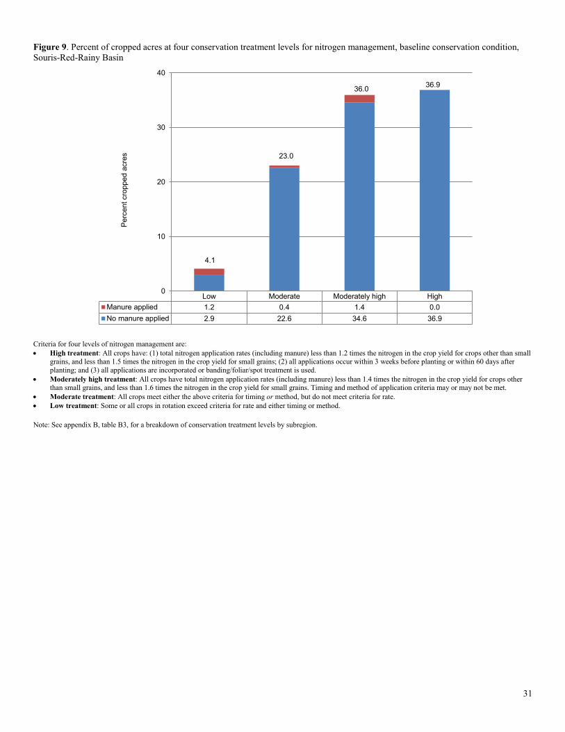
Figure 9. Percent of cropped acres at four conservation treatment levels for nitrogen management, baseline conservation condition, Souris-Red-Rainy Basin

Criteria for four levels of nitrogen management are: • High treatment: All crops have: (1) total nitrogen application rates (including manure) less than 1.2 times the nitrogen in the crop yield for crops other than small

grains, and less than 1.5 times the nitrogen in the crop yield for small grains; (2) all applications occur within 3 weeks before planting or within 60 days after planting; and (3) all applications are incorporated or banding/foliar/spot treatment is used.

• Moderately high treatment: All crops have total nitrogen application rates (including manure) less than 1.4 times the nitrogen in the crop yield for crops other than small grains, and less than 1.6 times the nitrogen in the crop yield for small grains. Timing and method of application criteria may or may not be met.

• Moderate treatment: All crops meet either the above criteria for timing or method, but do not meet criteria for rate. • Low treatment: Some or all crops in rotation exceed criteria for rate and either timing or method. Note: See appendix B, table B3, for a breakdown of conservation treatment levels by subregion.

Low Moderate Moderately high HighManure applied 1.2 0.4 1.4 0.0No manure applied 2.9 22.6 34.6 36.9

4.1

23.0

36.0 36.9

0

10

20

30

40

Per

cent

cro

pped

acr

es

31

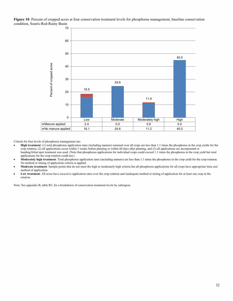
Figure 10. Percent of cropped acres at four conservation treatment levels for phosphorus management, baseline conservation condition, Souris-Red-Rainy Basin

Criteria for four levels of phosphorus management are: • High treatment: (1) total phosphorus application rates (including manure) summed over all crops are less than 1.1 times the phosphorus in the crop yields for the

crop rotation, (2) all applications occur within 3 weeks before planting or within 60 days after planting, and (3) all applications are incorporated or banding/foliar/spot treatment was used. (Note that phosphorus applications for individual crops could exceed 1.1 times the phosphorus in the crop yield but total applications for the crop rotation could not.)

• Moderately high treatment: Total phosphorus application rates (including manure) are less than 1.1 times the phosphorus in the crop yield for the crop rotation. No method or timing of application criteria is applied.

• Moderate treatment: Sample points that do not meet the high or moderately high criteria but all phosphorus applications for all crops have appropriate time and method of application.

• Low treatment: All acres have excessive application rates over the crop rotation and inadequate method or timing of application for at least one crop in the rotation.

Note: See appendix B, table B3, for a breakdown of conservation treatment levels by subregion.

Low Moderate Moderately high HighManure applied 2.4 0.0 0.6 0.0No manure applied 16.1 24.6 11.2 45.0

18.5

24.6

11.9

45.0

0

10

20

30

40

50

60

70

Per

cent

of c

ropp

ed a

cres

32

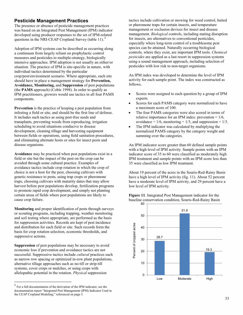
Pesticide Management Practices The presence or absence of pesticide management practices was based on an Integrated Pest Management (IPM) indicator developed using producer responses to the set of IPM-related questions in the NRI-CEAP Cropland Survey (table 11).8F

9 Adoption of IPM systems can be described as occurring along a continuum from largely reliant on prophylactic control measures and pesticides to multiple-strategy, biologically intensive approaches. IPM adoption is not usually an either/or situation. The practice of IPM is site-specific in nature, with individual tactics determined by the particular crop/pest/environment scenario. Where appropriate, each site should have in place a management strategy for Prevention, Avoidance, Monitoring, and Suppression of pest populations (the PAMS approach) (Coble 1998). In order to qualify as IPM practitioners, growers would use tactics in all four PAMS components. Prevention is the practice of keeping a pest population from infesting a field or site, and should be the first line of defense. It includes such tactics as using pest-free seeds and transplants, preventing weeds from reproducing, irrigation scheduling to avoid situations conducive to disease development, cleaning tillage and harvesting equipment between fields or operations, using field sanitation procedures, and eliminating alternate hosts or sites for insect pests and disease organisms. Avoidance may be practiced when pest populations exist in a field or site but the impact of the pest on the crop can be avoided through some cultural practice. Examples of avoidance tactics include crop rotation in which the crop of choice is not a host for the pest, choosing cultivars with genetic resistance to pests, using trap crops or pheromone traps, choosing cultivars with maturity dates that may allow harvest before pest populations develop, fertilization programs to promote rapid crop development, and simply not planting certain areas of fields where pest populations are likely to cause crop failure. Monitoring and proper identification of pests through surveys or scouting programs, including trapping, weather monitoring and soil testing where appropriate, are performed as the basis for suppression activities. Records are kept of pest incidence and distribution for each field or site. Such records form the basis for crop rotation selection, economic thresholds, and suppressive actions. Suppression of pest populations may be necessary to avoid economic loss if prevention and avoidance tactics are not successful. Suppressive tactics include cultural practices such as narrow row spacing or optimized in-row plant populations, alternative tillage approaches such as no-till or strip-till systems, cover crops or mulches, or using crops with allelopathic potential in the rotation. Physical suppression

9 For a full documentation of the derivation of the IPM indicator, see the documentation report “Integrated Pest Management (IPM) Indicator Used in the CEAP Cropland Modeling;” referenced on page 5.

tactics include cultivation or mowing for weed control, baited or pheromone traps for certain insects, and temperature management or exclusion devices for insect and disease management. Biological controls, including mating disruption for insects, are alternatives to conventional pesticides, especially where long-term control of a troublesome pest species can be attained. Naturally occurring biological controls, where they exist, are important IPM tools. Chemical pesticides are applied as a last resort in suppression systems using a sound management approach, including selection of pesticides with low risk to non-target organisms. An IPM index was developed to determine the level of IPM activity for each sample point. The index was constructed as follows. • Scores were assigned to each question by a group of IPM

experts. • Scores for each PAMS category were normalized to have

a maximum score of 100. • The four PAMS categories were also scored in terms of

relative importance for an IPM index: prevention = 1/6, avoidance = 1/6, monitoring = 1/3, and suppression = 1/3.

• The IPM indicator was calculated by multiplying the normalized PAMS category by the category weight and summing over the categories.

An IPM indicator score greater than 60 defined sample points with a high level of IPM activity. Sample points with an IPM indicator score of 35 to 60 were classified as moderately high IPM treatment and sample points with an IPM score less than 35 were classified as low IPM treatment. About 19 percent of the acres in the Souris-Red-Rainy Basin have a high level of IPM activity (fig. 11). About 52 percent have a moderate level of IPM activity, and 29 percent have a low level of IPM activity. Figure 11. Integrated Pest Management indicator for the baseline conservation condition, Souris-Red-Rainy Basin

28.7

51.9

19.3

0

10

20

30

40

50

60

Low Moderate High

Per

cent

of c

ropp

ed a

cres

33

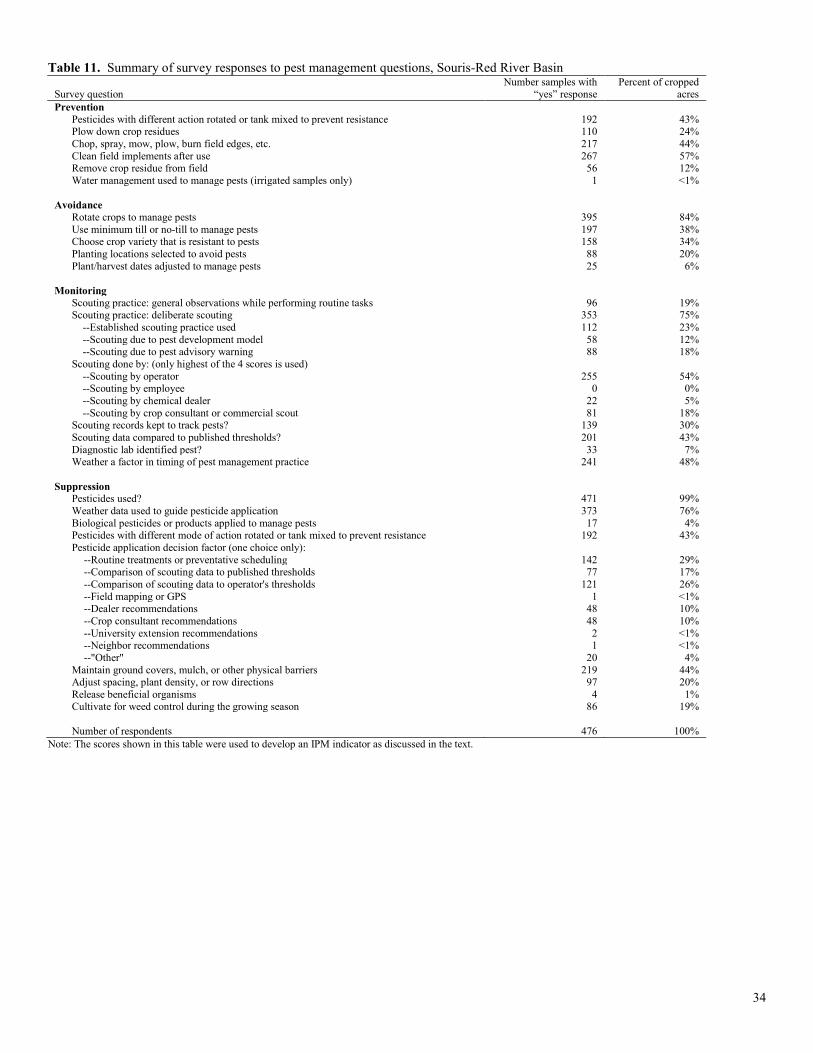
Table 11. Summary of survey responses to pest management questions, Souris-Red River Basin

Survey question Number samples with

“yes” response Percent of cropped

acres Prevention

Pesticides with different action rotated or tank mixed to prevent resistance 192 43% Plow down crop residues 110 24% Chop, spray, mow, plow, burn field edges, etc. 217 44% Clean field implements after use 267 57% Remove crop residue from field 56 12% Water management used to manage pests (irrigated samples only) 1 <1%

Avoidance

Rotate crops to manage pests 395 84% Use minimum till or no-till to manage pests 197 38% Choose crop variety that is resistant to pests 158 34% Planting locations selected to avoid pests 88 20% Plant/harvest dates adjusted to manage pests 25 6%

Monitoring

Scouting practice: general observations while performing routine tasks 96 19% Scouting practice: deliberate scouting 353 75% --Established scouting practice used 112 23% --Scouting due to pest development model 58 12% --Scouting due to pest advisory warning 88 18% Scouting done by: (only highest of the 4 scores is used) --Scouting by operator 255 54% --Scouting by employee 0 0% --Scouting by chemical dealer 22 5% --Scouting by crop consultant or commercial scout 81 18% Scouting records kept to track pests? 139 30% Scouting data compared to published thresholds? 201 43% Diagnostic lab identified pest? 33 7% Weather a factor in timing of pest management practice 241 48%

Suppression

Pesticides used? 471 99% Weather data used to guide pesticide application 373 76% Biological pesticides or products applied to manage pests 17 4% Pesticides with different mode of action rotated or tank mixed to prevent resistance 192 43% Pesticide application decision factor (one choice only):

--Routine treatments or preventative scheduling 142 29% --Comparison of scouting data to published thresholds 77 17% --Comparison of scouting data to operator's thresholds 121 26% --Field mapping or GPS 1 <1% --Dealer recommendations 48 10% --Crop consultant recommendations 48 10% --University extension recommendations 2 <1% --Neighbor recommendations 1 <1% --"Other" 20 4%

Maintain ground covers, mulch, or other physical barriers 219 44% Adjust spacing, plant density, or row directions 97 20% Release beneficial organisms 4 1% Cultivate for weed control during the growing season 86 19% Number of respondents 476 100%

Note: The scores shown in this table were used to develop an IPM indicator as discussed in the text.

34

Conservation Cover Establishment Establishing long-term cover of grass, forbs, or trees on a site provides the maximum protection against soil erosion. Conservation cover establishment is often used on cropland with soils that are vulnerable to erosion or leaching. The practice is also effective for sites that are adjacent to waterways, ponds, and lakes. Because these covers do not require annual applications of fertilizer and pesticides, this long-term conserving cover practice greatly reduces the loss of nitrogen and phosphorus from the site, and nearly eliminates pesticide loss. Because conservation covers are not harvested, they generate organic material that decomposes and increases soil organic carbon. For this study, the effect of a long-term conserving cover practice was estimated using acres enrolled in the General Signup of the CRP. The CRP General Signup is a voluntary program in which producers with eligible land enter into 10- to 15-year contracts to establish long-term cover to reduce soil erosion, improve water quality, and enhance wildlife habitat. Landowners receive annual rental payments and cost-share assistance for establishing and maintaining permanent vegetative cover. To be eligible for enrollment in the CRP General Signup, the field (or tract) must meet specified crop history criteria.

Other factors governing enrollment in the CRP include natural resource-based eligibility criteria, an Environmental Benefits Index (EBI) used to compare and rank enrollment offers, acreage limits, and upper limits on the proportion of a county’s cropland that can be enrolled (USDA Farm Service Agency 2004; Wiebe and Gollehon 2006). Initially, the eligibility criteria included only soil erosion rates and inherent soil erodibility. During the 1990s and to date, the eligibility criteria have continued to evolve, with increasing emphasis placed on issues other than soil erodibility. For contract offer ranking, weight was given to proposals that also benefited wildlife, air and water quality, and other environmental concerns. As of 2003, about 31.5 million acres were enrolled in the CRP General Signup nationally, including about 2.3 million in the Souris-Red-Rainy Basin (USDA/NRCS 2007). Approximately 29 percent of the cropland acres enrolled in the CRP in the Souris-Red-Rainy Basin are classified as highly erodible land. The inclusion of non-highly erodible land is due to both the expansion of enrollment eligibility criteria beyond soil erosion issues and the fact that farmers were allowed to enroll entire fields in the CRP if a specified portion of the field (varied by signup and eligibility criterion) met the criteria. In the Souris-Red-Rainy Basin, 70 percent of the CRP land is planted to introduced grasses and 5 percent to native grasses. An additional 23 percent has plantings specifically to support wildlife and about 2 percent is planted to trees. The plantings designated in the NRI database for each sample point were simulated in the APEX model. However, in all cases the simulated cover was a mix of species and all points included at least one grass and one clover species.

35

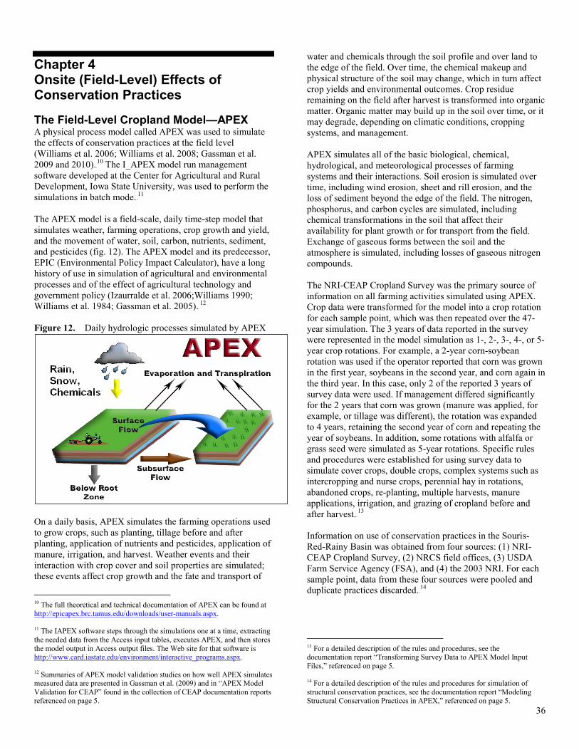
Chapter 4 Onsite (Field-Level) Effects of Conservation Practices The Field-Level Cropland Model—APEX A physical process model called APEX was used to simulate the effects of conservation practices at the field level (Williams et al. 2006; Williams et al. 2008; Gassman et al. 2009 and 2010).9F

10 The I_APEX model run management software developed at the Center for Agricultural and Rural Development, Iowa State University, was used to perform the simulations in batch mode.10F

11 The APEX model is a field-scale, daily time-step model that simulates weather, farming operations, crop growth and yield, and the movement of water, soil, carbon, nutrients, sediment, and pesticides (fig. 12). The APEX model and its predecessor, EPIC (Environmental Policy Impact Calculator), have a long history of use in simulation of agricultural and environmental processes and of the effect of agricultural technology and government policy (Izaurralde et al. 2006;Williams 1990; Williams et al. 1984; Gassman et al. 2005).11F

12

Figure 12. Daily hydrologic processes simulated by APEX

On a daily basis, APEX simulates the farming operations used to grow crops, such as planting, tillage before and after planting, application of nutrients and pesticides, application of manure, irrigation, and harvest. Weather events and their interaction with crop cover and soil properties are simulated; these events affect crop growth and the fate and transport of

10 The full theoretical and technical documentation of APEX can be found at http://epicapex.brc.tamus.edu/downloads/user-manuals.aspx. 11 The IAPEX software steps through the simulations one at a time, extracting the needed data from the Access input tables, executes APEX, and then stores the model output in Access output files. The Web site for that software is http://www.card.iastate.edu/environment/interactive_programs.aspx. 12 Summaries of APEX model validation studies on how well APEX simulates measured data are presented in Gassman et al. (2009) and in “APEX Model Validation for CEAP” found in the collection of CEAP documentation reports referenced on page 5.

water and chemicals through the soil profile and over land to the edge of the field. Over time, the chemical makeup and physical structure of the soil may change, which in turn affect crop yields and environmental outcomes. Crop residue remaining on the field after harvest is transformed into organic matter. Organic matter may build up in the soil over time, or it may degrade, depending on climatic conditions, cropping systems, and management. APEX simulates all of the basic biological, chemical, hydrological, and meteorological processes of farming systems and their interactions. Soil erosion is simulated over time, including wind erosion, sheet and rill erosion, and the loss of sediment beyond the edge of the field. The nitrogen, phosphorus, and carbon cycles are simulated, including chemical transformations in the soil that affect their availability for plant growth or for transport from the field. Exchange of gaseous forms between the soil and the atmosphere is simulated, including losses of gaseous nitrogen compounds. The NRI-CEAP Cropland Survey was the primary source of information on all farming activities simulated using APEX. Crop data were transformed for the model into a crop rotation for each sample point, which was then repeated over the 47-year simulation. The 3 years of data reported in the survey were represented in the model simulation as 1-, 2-, 3-, 4-, or 5-year crop rotations. For example, a 2-year corn-soybean rotation was used if the operator reported that corn was grown in the first year, soybeans in the second year, and corn again in the third year. In this case, only 2 of the reported 3 years of survey data were used. If management differed significantly for the 2 years that corn was grown (manure was applied, for example, or tillage was different), the rotation was expanded to 4 years, retaining the second year of corn and repeating the year of soybeans. In addition, some rotations with alfalfa or grass seed were simulated as 5-year rotations. Specific rules and procedures were established for using survey data to simulate cover crops, double crops, complex systems such as intercropping and nurse crops, perennial hay in rotations, abandoned crops, re-planting, multiple harvests, manure applications, irrigation, and grazing of cropland before and after harvest.12F

13 Information on use of conservation practices in the Souris-Red-Rainy Basin was obtained from four sources: (1) NRI-CEAP Cropland Survey, (2) NRCS field offices, (3) USDA Farm Service Agency (FSA), and (4) the 2003 NRI. For each sample point, data from these four sources were pooled and duplicate practices discarded.13F

14

13 For a detailed description of the rules and procedures, see the documentation report “Transforming Survey Data to APEX Model Input Files,” referenced on page 5. 14 For a detailed description of the rules and procedures for simulation of structural conservation practices, see the documentation report “Modeling Structural Conservation Practices in APEX,” referenced on page 5.

36

Simulating the No-Practice Scenario The purpose of the no-practice scenario is to provide an estimate of sediment, nutrient, and pesticide loss from farm fields under conditions without the use of conservation practices. The benefits of conservation practices in use within the Souris-Red-Rainy Basin were estimated by contrasting model output from the no-practice scenario to model output from the baseline conservation condition (2003–06). The only difference between the no-practice scenario and the baseline conservation condition is that the conservation practices are removed or their effects are reversed in the no-practice scenario simulations. There were usually several alternatives that could be used to represent “no practices.” The no-practice representations derived for use in this study conformed to the following guidelines. • Consistency: It is impossible to determine what an

individual farmer would be doing if he or she had not adopted certain practices, so it is important to represent all practices on all sample points in a consistent manner that is based on the intended purpose of each practice.

• Simplicity: Complex rules for assigning “no-practice”

activities lead to complex explanations that are difficult to substantiate and sometimes difficult to explain and accept. Complexity would not only complicate the modeling process but also hamper the interpretation of results.

• Historical context avoided: The no-practice scenario is a

technological step backward for conservation, not a chronological step back to a prior era when conservation practices were not used. Although the advent of certain conservation technologies can be dated, the adoption of technology is gradual, regionally diverse, and ongoing. It is also important to retain the overall crop mix in the region, as it in part reflects today’s market forces. Therefore, moving the clock back to 1950s (or any other time period) agriculture is not the goal of the no-practice scenario. Taking away the conservation ethic is the goal.

• Moderation: The no-practice scenario should provide a

reasonable level of inadequate conservation so that a reasonable benefit can be determined, where warranted, but not so severe as to generate exaggerated conservation gains by simulating the worst-case condition. Tremendous benefits could be generated if, for example, nutrients were applied at twice the recommended rates with poor timing or application methods in the no-practice simulation. Similarly, large erosion benefits could be calculated if the no-practice representation for tillage was fall plowing with moldboard plows and heavy disking, which was once common but today would generally be considered economically inefficient.

• Maintenance of crop yield or efficacy. It is impossible

to avoid small changes in crop yields, but care was taken to avoid no-practice representations that would significantly change crop yields and regional production capabilities. The same guideline was followed for pest

control—the suite of pesticides used was not adjusted in the no-practice scenario because of the likelihood that alternative pesticides would not be as effective and would result in lower yields under actual conditions.

A deliberate effort was made to adhere to these guidelines to the same degree for all conservation practices so that the overall level of representation would be equally moderate for all practices. Table 12 summarizes the adjustments to conservation practices used in simulation of the no-practice scenario. No-practice representation of structural practices The no-practice field condition for structural practices is simply the removal of the structural practices from the modeling process. In addition, the soil condition is changed from “Good” to “Poor” for the determination of the runoff curve number for erosion prediction. Overland flow. This group includes such practices as terraces and contouring which slow the flow of water across the field. For the practices affecting overland flow of water and therefore the P factor of the USLE-based equations, the P factor was increased to 1. Slope length is also changed for practices such as terraces to reflect the absence of these slope-interrupting practices. Concentrated flow. This group of practices is designed to address channelized flow and includes grassed waterways and grade stabilization structures. These practices are designed to prevent areas of concentrated flow from developing gullies or to stabilize gullies that have developed. The no-practice protocol for these practices removes the structure or waterway and replaces it with a “ditch” as a separate subarea. This ditch, or channel, represents a gully; however, the only sediment contributions from the gully will come from downcutting. Headcutting and sloughing of the sides are not simulated in APEX. Edge of field. These practices include buffers, filters, and other practices that occur outside the primary production area and act to mitigate the losses from the field. The no-practice protocol removes these areas and their management. When the practices are removed, the slope length is also restored to the undisturbed length that it would be if the practices were not in place. (When simulating a buffer in APEX, the slope length reported in the NRI is adjusted.)

Wind control. Practices such as windbreaks or shelterbelts, cross wind ridges, stripcropping or trap strips, and hedgerows are examples of practices used for wind control. The unsheltered distance reflects the dimensions of the field as modeled, 400 meters or 1,312 feet. Any practices reducing the unsheltered distance are removed and the unsheltered distance set to 400 meters.

37

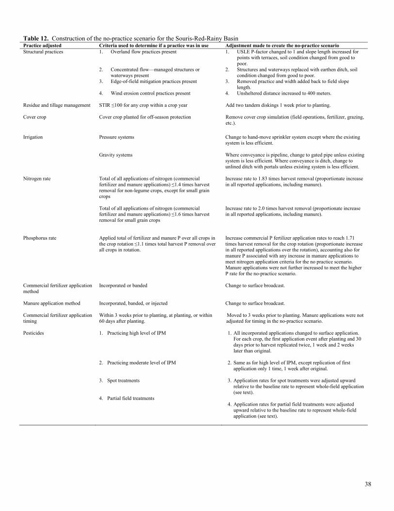
Table 12. Construction of the no-practice scenario for the Souris-Red-Rainy Basin Practice adjusted Criteria used to determine if a practice was in use Adjustment made to create the no-practice scenario Structural practices 1. Overland flow practices present

2. Concentrated flow—managed structures or

waterways present 3. Edge-of-field mitigation practices present 4. Wind erosion control practices present

1. USLE P-factor changed to 1 and slope length increased for points with terraces, soil condition changed from good to poor.

2. Structures and waterways replaced with earthen ditch, soil condition changed from good to poor.

3. Removed practice and width added back to field slope length.

4. Unsheltered distance increased to 400 meters. Residue and tillage management

STIR ≤100 for any crop within a crop year

Add two tandem diskings 1 week prior to planting.

Cover crop

Cover crop planted for off-season protection Remove cover crop simulation (field operations, fertilizer, grazing, etc.).

Irrigation Pressure systems Gravity systems

Change to hand-move sprinkler system except where the existing system is less efficient. Where conveyance is pipeline, change to gated pipe unless existing system is less efficient. Where conveyance is ditch, change to unlined ditch with portals unless existing system is less efficient.

Nitrogen rate

Total of all applications of nitrogen (commercial fertilizer and manure applications) ≤1.4 times harvest removal for non-legume crops, except for small grain crops Total of all applications of nitrogen (commercial fertilizer and manure applications) ≤1.6 times harvest removal for small grain crops

Increase rate to 1.83 times harvest removal (proportionate increase in all reported applications, including manure). Increase rate to 2.0 times harvest removal (proportionate increase in all reported applications, including manure).

Phosphorus rate Applied total of fertilizer and manure P over all crops in the crop rotation ≤1.1 times total harvest P removal over all crops in rotation.

Increase commercial P fertilizer application rates to reach 1.71 times harvest removal for the crop rotation (proportionate increase in all reported applications over the rotation), accounting also for manure P associated with any increase in manure applications to meet nitrogen application criteria for the no practice scenario. Manure applications were not further increased to meet the higher P rate for the no-practice scenario.

Commercial fertilizer application method

Incorporated or banded

Change to surface broadcast.

Manure application method Incorporated, banded, or injected

Change to surface broadcast.

Commercial fertilizer application timing

Within 3 weeks prior to planting, at planting, or within 60 days after planting.

Moved to 3 weeks prior to planting. Manure applications were not adjusted for timing in the no-practice scenario.

Pesticides

1. Practicing high level of IPM 2. Practicing moderate level of IPM 3. Spot treatments 4. Partial field treatments

1. All incorporated applications changed to surface application. For each crop, the first application event after planting and 30 days prior to harvest replicated twice, 1 week and 2 weeks later than original.

2. Same as for high level of IPM, except replication of first

application only 1 time, 1 week after original.

3. Application rates for spot treatments were adjusted upward relative to the baseline rate to represent whole-field application (see text).

4. Application rates for partial field treatments were adjusted

upward relative to the baseline rate to represent whole-field application (see text).

38

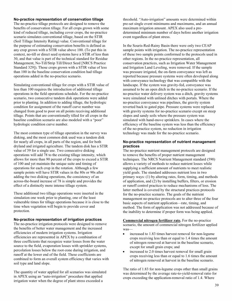
No-practice representation of conservation tillage The no-practice tillage protocols are designed to remove the benefits of conservation tillage. For all crops grown with some kind of reduced tillage, including cover crops, the no-practice scenario simulates conventional tillage, based on the STIR (Soil Tillage Intensity Rating) value. Conventional tillage for the purpose of estimating conservation benefits is defined as any crop grown with a STIR value above 100. (To put this in context, no-till or direct seed systems have a STIR of less than 30, and that value is part of the technical standard for Residue Management, No-Till/Strip Till/Direct Seed [NRCS Practice Standard 329]). Those crops grown with a STIR value of less than 100 in the baseline conservation condition had tillage operations added in the no-practice scenario. Simulating conventional tillage for crops with a STIR value of less than 100 requires the introduction of additional tillage operations in the field operations schedule. For the no-practice scenario, two consecutive tandem disk operations were added prior to planting. In addition to adding tillage, the hydrologic condition for assignment of the runoff curve number was changed from good to poor on all points receiving additional tillage. Points that are conventionally tilled for all crops in the baseline condition scenario are also modeled with a “poor” hydrologic condition curve number. The most common type of tillage operation in the survey was disking, and the most common disk used was a tandem disk for nearly all crops, in all parts of the region, and for both dryland and irrigated agriculture. The tandem disk has a STIR value of 39 for a single use. Two consecutive disking operations will add 78 to the existing tillage intensity, which allows for more than 90 percent of the crops to exceed a STIR of 100 and yet maintain the unique suite and timing of operations for each crop in the rotation. Although a few sample points will have STIR values in the 80s or 90s after adding the two disking operations, the consistency of an across-the-board increase of 78 is simple and provides the effect of a distinctly more intense tillage system. These additional two tillage operations were inserted in the simulation one week prior to planting, one of the least vulnerable times for tillage operations because it is close to the time when vegetation will begin to provide cover and protection. No-practice representation of irrigation practices The no-practice irrigation protocols were designed to remove the benefits of better water management and the increased efficiencies of modern irrigation systems. Irrigation efficiencies are represented in APEX by a combination of three coefficients that recognize water losses from the water source to the field, evaporation losses with sprinkler systems, percolation losses below the root-zone during irrigation, and runoff at the lower end of the field. These coefficients are combined to form an overall system efficiency that varies with soil type and land slope. The quantity of water applied for all scenarios was simulated in APEX using an “auto-irrigation” procedure that applied irrigation water when the degree of plant stress exceeded a

threshold. “Auto-irrigation” amounts were determined within pre-set single event minimums and maximums, and an annual maximum irrigation amount. APEX also used a pre-determined minimum number of days before another irrigation event regardless of plant stress. In the Souris-Red-Rainy Basin there were only two CEAP sample points with irrigation. The no-practice representation of these two sample points conformed to the protocols used in other regions. In the no-practice representation, all conservation practices, such as Irrigation Water Management and Irrigation Land Leveling, were removed. If the sample was pressure irrigated, the on-farm conveyance was left as reported because pressure systems were often developed along with conveyance technology that was compatible with the landscape. If the system was gravity-fed, conveyance was assumed to be an open ditch in the no-practice scenario. If the no-practice water delivery system was a ditch, gravity systems were simulated with unlined ditches with portals. Where the no-practice conveyance was pipelines, the gravity system reverted back to gated pipe. Pressure systems were replaced with gravity systems for no-practice scenario except on steep slopes and sandy soils where the pressure system was simulated with hand-move sprinklers. In cases where the efficiency of the baseline system was less than the efficiency of the no-practice system, no reduction in irrigation technology was made for the no-practice scenario. No-practice representation of nutrient management practices The no-practice nutrient management protocols are designed to remove the benefits of proper nutrient management techniques. The NRCS Nutrient Management standard (590) allows a variety of methods to reduce nutrient losses while supplying a sufficient amount of nutrients to meet realistic yield goals. The standard addresses nutrient loss in two primary ways: (1) by altering rates, form, timing, and methods of application, and (2) by installing buffers, filters, or erosion or runoff control practices to reduce mechanisms of loss. The latter method is covered by the structural practices protocols for the no-practice scenario. The goals of the nutrient management no-practice protocols are to alter three of the four basic aspects of nutrient application—rate, timing, and method. The form of application was not addressed because of the inability to determine if proper form was being applied. Commercial nitrogen fertilizer rate. For the no-practice scenario, the amount of commercial nitrogen fertilizer applied was— • increased to 1.83 times harvest removal for non-legume

crops receiving less than or equal to 1.4 times the amount of nitrogen removed at harvest in the baseline scenario, except for small grain crops; and

• increased to 2.0 times harvest removal for small grain crops receiving less than or equal to 1.6 times the amount of nitrogen removed at harvest in the baseline scenario.

The ratio of 1.83 for non-legume crops other than small grains was determined by the average rate-to-yield-removal ratio for crops exceeding the application-removal ratio of 1.4. Where

39

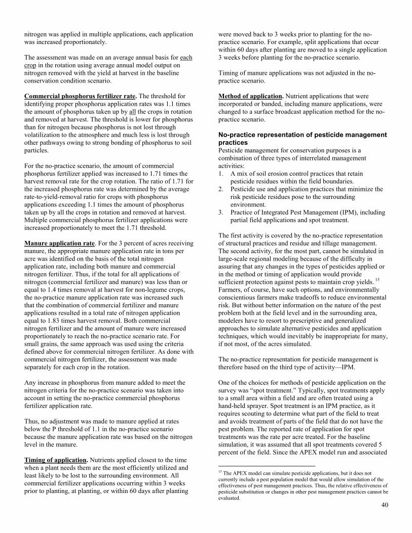
nitrogen was applied in multiple applications, each application was increased proportionately. The assessment was made on an average annual basis for each crop in the rotation using average annual model output on nitrogen removed with the yield at harvest in the baseline conservation condition scenario. Commercial phosphorus fertilizer rate. The threshold for identifying proper phosphorus application rates was 1.1 times the amount of phosphorus taken up by all the crops in rotation and removed at harvest. The threshold is lower for phosphorus than for nitrogen because phosphorus is not lost through volatilization to the atmosphere and much less is lost through other pathways owing to strong bonding of phosphorus to soil particles. For the no-practice scenario, the amount of commercial phosphorus fertilizer applied was increased to 1.71 times the harvest removal rate for the crop rotation. The ratio of 1.71 for the increased phosphorus rate was determined by the average rate-to-yield-removal ratio for crops with phosphorus applications exceeding 1.1 times the amount of phosphorus taken up by all the crops in rotation and removed at harvest. Multiple commercial phosphorus fertilizer applications were increased proportionately to meet the 1.71 threshold. Manure application rate. For the 3 percent of acres receiving manure, the appropriate manure application rate in tons per acre was identified on the basis of the total nitrogen application rate, including both manure and commercial nitrogen fertilizer. Thus, if the total for all applications of nitrogen (commercial fertilizer and manure) was less than or equal to 1.4 times removal at harvest for non-legume crops, the no-practice manure application rate was increased such that the combination of commercial fertilizer and manure applications resulted in a total rate of nitrogen application equal to 1.83 times harvest removal. Both commercial nitrogen fertilizer and the amount of manure were increased proportionately to reach the no-practice scenario rate. For small grains, the same approach was used using the criteria defined above for commercial nitrogen fertilizer. As done with commercial nitrogen fertilizer, the assessment was made separately for each crop in the rotation. Any increase in phosphorus from manure added to meet the nitrogen criteria for the no-practice scenario was taken into account in setting the no-practice commercial phosphorus fertilizer application rate. Thus, no adjustment was made to manure applied at rates below the P threshold of 1.1 in the no-practice scenario because the manure application rate was based on the nitrogen level in the manure. Timing of application. Nutrients applied closest to the time when a plant needs them are the most efficiently utilized and least likely to be lost to the surrounding environment. All commercial fertilizer applications occurring within 3 weeks prior to planting, at planting, or within 60 days after planting

were moved back to 3 weeks prior to planting for the no-practice scenario. For example, split applications that occur within 60 days after planting are moved to a single application 3 weeks before planting for the no-practice scenario. Timing of manure applications was not adjusted in the no-practice scenario. Method of application. Nutrient applications that were incorporated or banded, including manure applications, were changed to a surface broadcast application method for the no-practice scenario. No-practice representation of pesticide management practices Pesticide management for conservation purposes is a combination of three types of interrelated management activities: 1. A mix of soil erosion control practices that retain

pesticide residues within the field boundaries. 2. Pesticide use and application practices that minimize the

risk pesticide residues pose to the surrounding environment.

3. Practice of Integrated Pest Management (IPM), including partial field applications and spot treatment.

The first activity is covered by the no-practice representation of structural practices and residue and tillage management. The second activity, for the most part, cannot be simulated in large-scale regional modeling because of the difficulty in assuring that any changes in the types of pesticides applied or in the method or timing of application would provide sufficient protection against pests to maintain crop yields.14F

15 Farmers, of course, have such options, and environmentally conscientious farmers make tradeoffs to reduce environmental risk. But without better information on the nature of the pest problem both at the field level and in the surrounding area, modelers have to resort to prescriptive and generalized approaches to simulate alternative pesticides and application techniques, which would inevitably be inappropriate for many, if not most, of the acres simulated. The no-practice representation for pesticide management is therefore based on the third type of activity—IPM. One of the choices for methods of pesticide application on the survey was “spot treatment.” Typically, spot treatments apply to a small area within a field and are often treated using a hand-held sprayer. Spot treatment is an IPM practice, as it requires scouting to determine what part of the field to treat and avoids treatment of parts of the field that do not have the pest problem. The reported rate of application for spot treatments was the rate per acre treated. For the baseline simulation, it was assumed that all spot treatments covered 5 percent of the field. Since the APEX model run and associated

15 The APEX model can simulate pesticide applications, but it does not currently include a pest population model that would allow simulation of the effectiveness of pest management practices. Thus, the relative effectiveness of pesticide substitution or changes in other pest management practices cannot be evaluated.

40

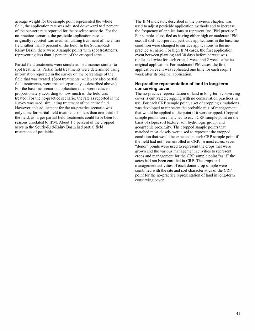
acreage weight for the sample point represented the whole field, the application rate was adjusted downward to 5 percent of the per-acre rate reported for the baseline scenario. For the no-practice scenario, the pesticide application rate as originally reported was used, simulating treatment of the entire field rather than 5 percent of the field. In the Souris-Red-Rainy Basin, there were 3 sample points with spot treatments, representing less than 1 percent of the cropped acres. Partial field treatments were simulated in a manner similar to spot treatments. Partial field treatments were determined using information reported in the survey on the percentage of the field that was treated. (Spot treatments, which are also partial field treatments, were treated separately as described above.) For the baseline scenario, application rates were reduced proportionately according to how much of the field was treated. For the no-practice scenario, the rate as reported in the survey was used, simulating treatment of the entire field. However, this adjustment for the no-practice scenario was only done for partial field treatments on less than one-third of the field, as larger partial field treatments could have been for reasons unrelated to IPM. About 1.5 percent of the cropped acres in the Souris-Red-Rainy Basin had partial field treatments of pesticides.

The IPM indicator, described in the previous chapter, was used to adjust pesticide application methods and to increase the frequency of applications to represent “no IPM practice.” For samples classified as having either high or moderate IPM use, all soil-incorporated pesticide applications in the baseline condition were changed to surface applications in the no-practice scenario. For high IPM cases, the first application event between planting and 30 days before harvest was replicated twice for each crop, 1 week and 2 weeks after its original application. For moderate IPM cases, the first application event was replicated one time for each crop, 1 week after its original application. No-practice representation of land in long-term conserving cover The no-practice representation of land in long-term conserving cover is cultivated cropping with no conservation practices in use. For each CRP sample point, a set of cropping simulations was developed to represent the probable mix of management that would be applied to the point if it were cropped. Cropped sample points were matched to each CRP sample point on the basis of slope, soil texture, soil hydrologic group, and geographic proximity. The cropped sample points that matched most closely were used to represent the cropped condition that would be expected at each CRP sample point if the field had not been enrolled in CRP. In most cases, seven “donor” points were used to represent the crops that were grown and the various management activities to represent crops and management for the CRP sample point “as if” the acres had not been enrolled in CRP. The crops and management activities of each donor crop sample were combined with the site and soil characteristics of the CRP point for the no-practice representation of land in long-term conserving cover.

41

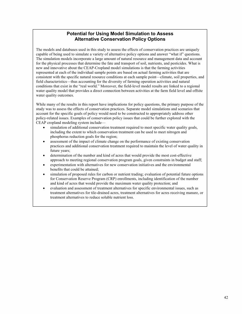
Potential for Using Model Simulation to Assess Alternative Conservation Policy Options

The models and databases used in this study to assess the effects of conservation practices are uniquely capable of being used to simulate a variety of alternative policy options and answer “what if” questions. The simulation models incorporate a large amount of natural resource and management data and account for the physical processes that determine the fate and transport of soil, nutrients, and pesticides. What is new and innovative about the CEAP-Cropland model simulations is that the farming activities represented at each of the individual sample points are based on actual farming activities that are consistent with the specific natural resource conditions at each sample point—climate, soil properties, and field characteristics—thus accounting for the diversity of farming operation activities and natural conditions that exist in the “real world.” Moreover, the field-level model results are linked to a regional water quality model that provides a direct connection between activities at the farm field level and offsite water quality outcomes. While many of the results in this report have implications for policy questions, the primary purpose of the study was to assess the effects of conservation practices. Separate model simulations and scenarios that account for the specific goals of policy would need to be constructed to appropriately address other policy-related issues. Examples of conservation policy issues that could be further explored with the CEAP cropland modeling system include—

• simulation of additional conservation treatment required to meet specific water quality goals, including the extent to which conservation treatment can be used to meet nitrogen and phosphorus reduction goals for the region;

• assessment of the impact of climate change on the performance of existing conservation practices and additional conservation treatment required to maintain the level of water quality in future years;

• determination of the number and kind of acres that would provide the most cost-effective approach to meeting regional conservation program goals, given constraints in budget and staff;

• experimentation with alternatives for new conservation initiatives and the environmental benefits that could be attained;

• simulation of proposed rules for carbon or nutrient trading; evaluation of potential future options for Conservation Reserve Program (CRP) enrollments, including identification of the number and kind of acres that would provide the maximum water quality protection; and

• evaluation and assessment of treatment alternatives for specific environmental issues, such as treatment alternatives for tile-drained acres, treatment alternatives for acres receiving manure, or treatment alternatives to reduce soluble nutrient loss.

42

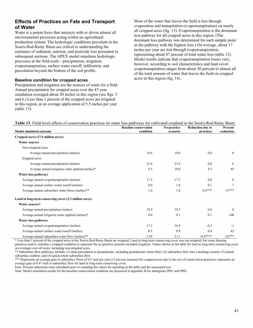
Effects of Practices on Fate and Transport of Water Water is a potent force that interacts with or drives almost all environmental processes acting within an agricultural production system. The hydrologic conditions prevalent in the Souris-Red-Rainy Basin are critical to understanding the estimates of sediment, nutrient, and pesticide loss presented in subsequent sections. The APEX model simulates hydrologic processes at the field scale—precipitation, irrigation, evapotranspiration, surface water runoff, infiltration, and percolation beyond the bottom of the soil profile. Baseline condition for cropped acres Precipitation and irrigation are the sources of water for a field. Annual precipitation for cropped acres over the 47-year simulation averaged about 20 inches in this region (see figs. 5 and 6.) Less than 1 percent of the cropped acres are irrigated in this region, at an average application of 5.5 inches per year (table 13).

Most of the water that leaves the field is lost through evaporation and transpiration (evapotranspiration) on nearly all cropped acres (fig. 13). Evapotranspiration is the dominant loss pathway for all cropped acres in this region. (The dominant loss pathway was determined for each sample point as the pathway with the highest loss.) On average, about 17 inches per year are lost through evapotranspiration, representing about 87 percent of total water loss (table 13). Model results indicate that evapotranspiration losses vary, however, according to soil characteristics and land cover; evapotranspiration ranges from about 50 percent to almost all of the total amount of water that leaves the field on cropped acres in this region (fig. 14).

Table 13. Field-level effects of conservation practices on water loss pathways for cultivated cropland in the Souris-Red-Rainy Basin

Model simulated outcome Baseline conservation

condition No-practice

scenario Reduction due to

practices Percent

reduction

Cropped acres (17.6 million acres) Water sources

Non-irrigated acres Average annual precipitation (inches) 19.6 19.6 0.0 0

Irrigated acres Average annual precipitation (inches) 23.4 23.4 0.0 0 Average annual irrigation water applied (inches)* 5.5 10.0 4.5 45

Water loss pathways Average annual evapotranspiration (inches) 17.3 17.3 0.0 0 Average annual surface water runoff (inches) 0.9 1.0 0.1 7 Average annual subsurface water flows (inches)** 1.6 1.4 -0.2*** -12***

Land in long-term conserving cover (2.3 million acres)

Water sources* Average annual precipitation (inches) 19.5 19.5 0.0 0 Average annual irrigation water applied (inches)* 0.0 0.1 0.1 100

Water loss pathways Average annual evapotranspiration (inches) 17.2 16.9 -0.2 -1 Average annual surface water runoff (inches) 0.5 0.9 0.4 42 Average annual subsurface water flow (inches)** 2.59 2.11 -0.47*** -22***

* Less than 1 percent of the cropped acres in the Souris-Red-Rainy Basin are irrigated. Land in long-term conserving cover was not irrigated, but some farming practices used to simulate a cropped condition to represent the no-practice scenario included irrigation. Values shown in the table for land in long-term conserving cover are averages over all acres, including non-irrigated acres. ** Subsurface flow pathways include: (1) deep percolation to groundwater, including groundwater return flow; (2) subsurface flow into a drainage system; (3) lateral subsurface outflow; and (4) quick-return subsurface flow. *** Represents an average gain in subsurface flows of 0.2 inch per year (12 percent increase) for cropped acres due to the use of conservation practices; represents an average gain of 0.47 inch in subsurface flow for land in long-term conserving cover. Note: Percent reductions were calculated prior to rounding the values for reporting in the table and the associated text. Note: Model simulation results for the baseline conservation condition are presented in appendix B for subregions 0901 and 0902.

43

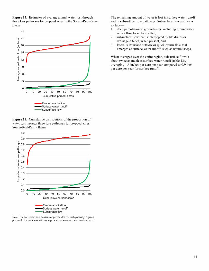
Figure 13. Estimates of average annual water lost through three loss pathways for cropped acres in the Souris-Red-Rainy Basin

Figure 14. Cumulative distributions of the proportion of water lost through three loss pathways for cropped acres, Souris-Red-Rainy Basin

Note: The horizontal axis consists of percentiles for each pathway; a given percentile for one curve will not represent the same acres on another curve.

The remaining amount of water is lost in surface water runoff and in subsurface flow pathways. Subsurface flow pathways include— 1. deep percolation to groundwater, including groundwater

return flow to surface water, 2. subsurface flow that is intercepted by tile drains or

drainage ditches, when present, and 3. lateral subsurface outflow or quick-return flow that

emerges as surface water runoff, such as natural seeps. When averaged over the entire region, subsurface flow is about twice as much as surface water runoff (table 13), averaging 1.6 inches per acre per year compared to 0.9 inch per acre per year for surface runoff.

0

3

6

9

12

15

18

21

24

0 10 20 30 40 50 60 70 80 90 100

Ave

rage

ann

ual w

ater

loss

(inc

hes)

Cumulative percent acres

EvapotranspirationSurface water runoffSubsurface flow

0.0

0.1

0.2

0.3

0.4

0.5

0.6

0.7

0.8

0.9

1.0

0 10 20 30 40 50 60 70 80 90 100

Pro

porti

on o

f wat

er lo

ss p

athw

ays

Cumulative percent acres

EvapotranspirationSurface water runoffSubsurface flow

44

Tile Drainage

Tile drainage flow is included in the water loss category “subsurface water flows” in this report. (See table 13.) Other components of subsurface water flow include: (1) deep percolation to groundwater, including groundwater return flow to surface water, (2) lateral subsurface flows intercepted by surface drainage ditches, and (3) lateral subsurface outflow or quick-return flow that emerges as surface water runoff, such as natural seeps. While the farmer survey provided information on whether or not the field with the CEAP sample point had tile drainage, tile drainage flow and loss of soluble nutrients in tile drainage water are not reported separately because other important information on the tile drainage characteristics were not covered in the survey. The missing information includes—

• the depth and spacing of the tile drainage field, • the extent of the tile drainage network, • the proportion of the field, or other fields, that benefited from the tile drainage system, and • the extent to which overland flow and subsurface flow from surrounding areas enters through tile surface inlets.

Without this additional information, it is not possible to accurately separate out the various components of subsurface flow when tile drainage systems are present. In the Souris-Red-Rainy Basin, only about 2 percent of the cropped acres have some portion of the field that is tile drained, according to the farmer survey.

45

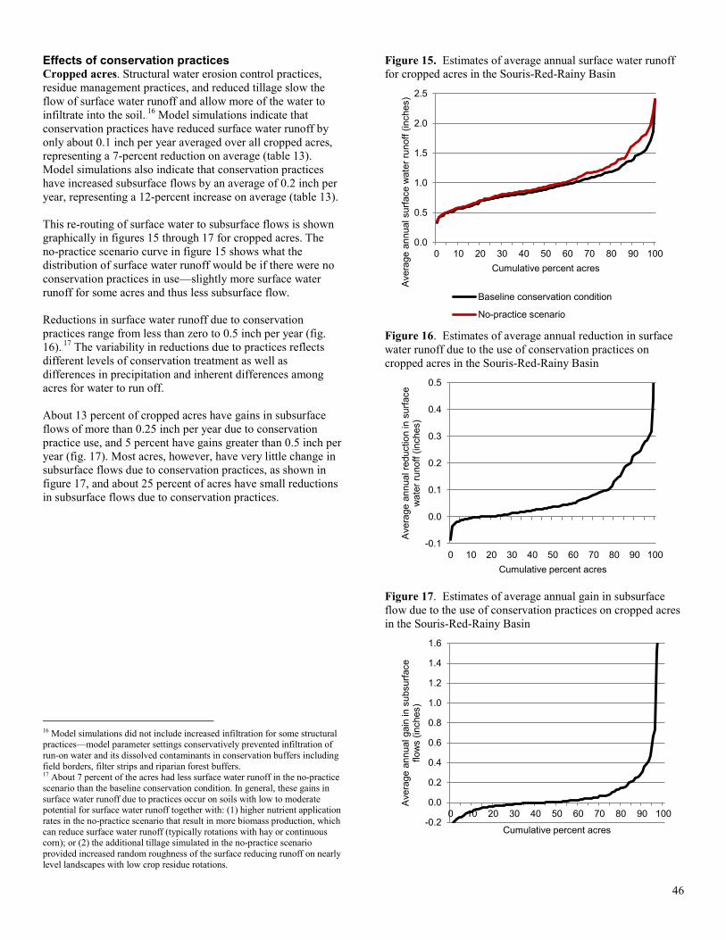
Effects of conservation practices Cropped acres. Structural water erosion control practices, residue management practices, and reduced tillage slow the flow of surface water runoff and allow more of the water to infiltrate into the soil.15F

16 Model simulations indicate that conservation practices have reduced surface water runoff by only about 0.1 inch per year averaged over all cropped acres, representing a 7-percent reduction on average (table 13). Model simulations also indicate that conservation practices have increased subsurface flows by an average of 0.2 inch per year, representing a 12-percent increase on average (table 13). This re-routing of surface water to subsurface flows is shown graphically in figures 15 through 17 for cropped acres. The no-practice scenario curve in figure 15 shows what the distribution of surface water runoff would be if there were no conservation practices in use—slightly more surface water runoff for some acres and thus less subsurface flow. Reductions in surface water runoff due to conservation practices range from less than zero to 0.5 inch per year (fig. 16).16F

17 The variability in reductions due to practices reflects different levels of conservation treatment as well as differences in precipitation and inherent differences among acres for water to run off. About 13 percent of cropped acres have gains in subsurface flows of more than 0.25 inch per year due to conservation practice use, and 5 percent have gains greater than 0.5 inch per year (fig. 17). Most acres, however, have very little change in subsurface flows due to conservation practices, as shown in figure 17, and about 25 percent of acres have small reductions in subsurface flows due to conservation practices.

16 Model simulations did not include increased infiltration for some structural practices—model parameter settings conservatively prevented infiltration of run-on water and its dissolved contaminants in conservation buffers including field borders, filter strips and riparian forest buffers. 17 About 7 percent of the acres had less surface water runoff in the no-practice scenario than the baseline conservation condition. In general, these gains in surface water runoff due to practices occur on soils with low to moderate potential for surface water runoff together with: (1) higher nutrient application rates in the no-practice scenario that result in more biomass production, which can reduce surface water runoff (typically rotations with hay or continuous corn); or (2) the additional tillage simulated in the no-practice scenario provided increased random roughness of the surface reducing runoff on nearly level landscapes with low crop residue rotations.

Figure 15. Estimates of average annual surface water runoff for cropped acres in the Souris-Red-Rainy Basin

Figure 16. Estimates of average annual reduction in surface water runoff due to the use of conservation practices on cropped acres in the Souris-Red-Rainy Basin

Figure 17. Estimates of average annual gain in subsurface flow due to the use of conservation practices on cropped acres in the Souris-Red-Rainy Basin

0.0

0.5

1.0

1.5

2.0

2.5

0 10 20 30 40 50 60 70 80 90 100

Ave

rage

ann

ual s

urfa

ce w

ater

runo

ff (in

ches

)

Cumulative percent acres

Baseline conservation condition

No-practice scenario

-0.1

0.0

0.1

0.2

0.3

0.4

0.5

0 10 20 30 40 50 60 70 80 90 100

Ave

rage

ann

ual r

educ

tion

in s

urfa

ce

wat

er ru

noff

(inch

es)

Cumulative percent acres

-0.2

0.0

0.2

0.4

0.6

0.8

1.0

1.2

1.4

1.6

0 10 20 30 40 50 60 70 80 90 100

Ave

rage

ann

ual g

ain

in s

ubsu

rface

flo

ws

(inch

es)

Cumulative percent acres

46

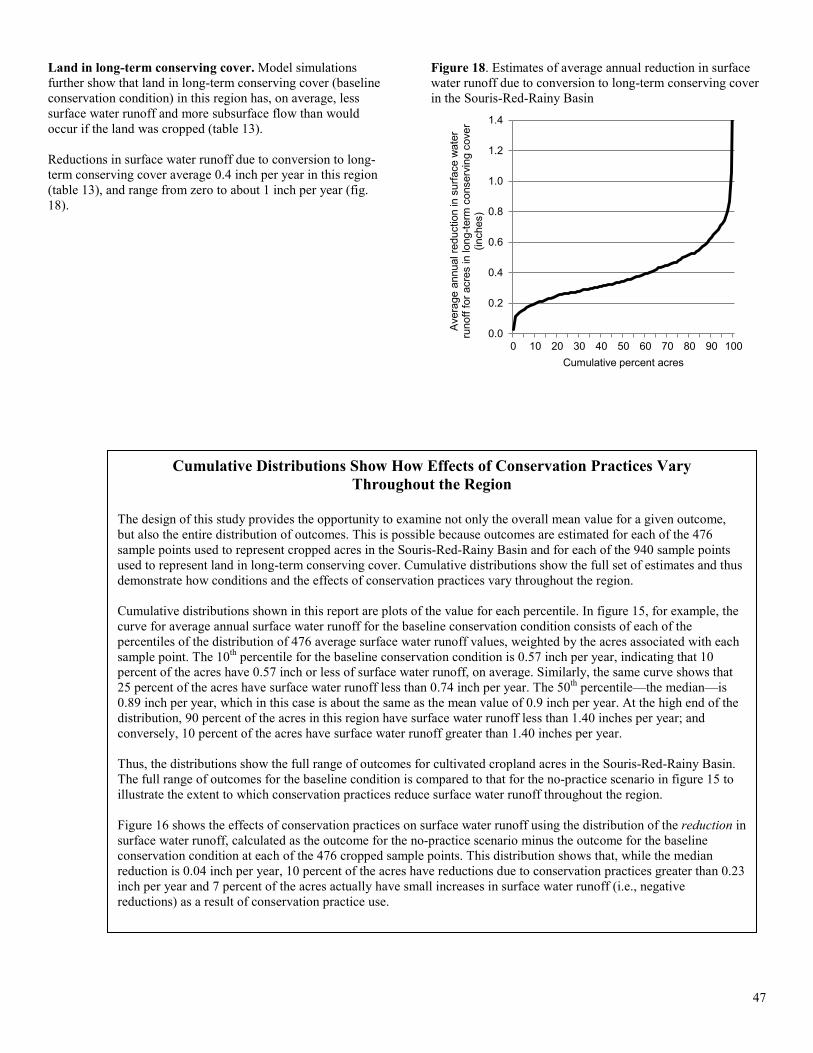
Land in long-term conserving cover. Model simulations further show that land in long-term conserving cover (baseline conservation condition) in this region has, on average, less surface water runoff and more subsurface flow than would occur if the land was cropped (table 13). Reductions in surface water runoff due to conversion to long-term conserving cover average 0.4 inch per year in this region (table 13), and range from zero to about 1 inch per year (fig. 18).

Figure 18. Estimates of average annual reduction in surface water runoff due to conversion to long-term conserving cover in the Souris-Red-Rainy Basin

0.0

0.2

0.4

0.6

0.8

1.0

1.2

1.4

0 10 20 30 40 50 60 70 80 90 100

Ave

rage

ann

ual r

educ

tion

in s

urfa

ce w

ater

ru

noff

for a

cres

in lo

ng-te

rm c

onse

rvin

g co

ver

(inch

es)

Cumulative percent acres

Cumulative Distributions Show How Effects of Conservation Practices Vary Throughout the Region

The design of this study provides the opportunity to examine not only the overall mean value for a given outcome, but also the entire distribution of outcomes. This is possible because outcomes are estimated for each of the 476 sample points used to represent cropped acres in the Souris-Red-Rainy Basin and for each of the 940 sample points used to represent land in long-term conserving cover. Cumulative distributions show the full set of estimates and thus demonstrate how conditions and the effects of conservation practices vary throughout the region. Cumulative distributions shown in this report are plots of the value for each percentile. In figure 15, for example, the curve for average annual surface water runoff for the baseline conservation condition consists of each of the percentiles of the distribution of 476 average surface water runoff values, weighted by the acres associated with each sample point. The 10th percentile for the baseline conservation condition is 0.57 inch per year, indicating that 10 percent of the acres have 0.57 inch or less of surface water runoff, on average. Similarly, the same curve shows that 25 percent of the acres have surface water runoff less than 0.74 inch per year. The 50th percentile—the median—is 0.89 inch per year, which in this case is about the same as the mean value of 0.9 inch per year. At the high end of the distribution, 90 percent of the acres in this region have surface water runoff less than 1.40 inches per year; and conversely, 10 percent of the acres have surface water runoff greater than 1.40 inches per year. Thus, the distributions show the full range of outcomes for cultivated cropland acres in the Souris-Red-Rainy Basin. The full range of outcomes for the baseline condition is compared to that for the no-practice scenario in figure 15 to illustrate the extent to which conservation practices reduce surface water runoff throughout the region. Figure 16 shows the effects of conservation practices on surface water runoff using the distribution of the reduction in surface water runoff, calculated as the outcome for the no-practice scenario minus the outcome for the baseline conservation condition at each of the 476 cropped sample points. This distribution shows that, while the median reduction is 0.04 inch per year, 10 percent of the acres have reductions due to conservation practices greater than 0.23 inch per year and 7 percent of the acres actually have small increases in surface water runoff (i.e., negative reductions) as a result of conservation practice use.

47

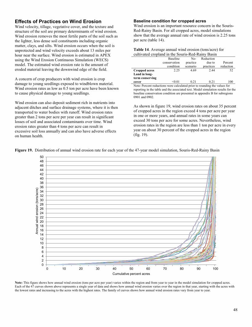
Effects of Practices on Wind Erosion Wind velocity, tillage, vegetative cover, and the texture and structure of the soil are primary determinants of wind erosion. Wind erosion removes the most fertile parts of the soil such as the lighter, less dense soil constituents including organic matter, clays, and silts. Wind erosion occurs when the soil is unprotected and wind velocity exceeds about 13 miles per hour near the surface. Wind erosion is estimated in APEX using the Wind Erosion Continuous Simulation (WECS) model. The estimated wind erosion rate is the amount of eroded material leaving the downwind edge of the field. A concern of crop producers with wind erosion is crop damage to young seedlings exposed to windblown material. Wind erosion rates as low as 0.5 ton per acre have been known to cause physical damage to young seedlings. Wind erosion can also deposit sediment rich in nutrients into adjacent ditches and surface drainage systems, where it is then transported to water bodies with runoff. Wind erosion rates greater than 2 tons per acre per year can result in significant losses of soil and associated contaminants over time. Wind erosion rates greater than 4 tons per acre can result in excessive soil loss annually and can also have adverse effects on human health.

Baseline condition for cropped acres Wind erosion is an important resource concern in the Souris-Red-Rainy Basin. For all cropped acres, model simulations show that the average annual rate of wind erosion is 2.25 tons per acre (table 14). Table 14. Average annual wind erosion (tons/acre) for cultivated cropland in the Souris-Red-Rainy Basin

Baseline conservation

condition

No-practice scenario

Reduction due to

practices Percent

reduction Cropped acres 2.25 4.69 2.44 52 Land in long-term conserving cover <0.01 0.21 0.21 100 Note: Percent reductions were calculated prior to rounding the values for reporting in the table and the associated text. Model simulation results for the baseline conservation condition are presented in appendix B for subregions 0901 and 0902. As shown in figure 19, wind erosion rates on about 35 percent of cropped acres in the region exceed 4 tons per acre per year in one or more years, and annual rates in some years can exceed 30 tons per acre for some acres. Nevertheless, wind erosion rates in the region are less than 1 ton per acre in every year on about 30 percent of the cropped acres in the region (fig. 19).

Figure 19. Distribution of annual wind erosion rate for each year of the 47-year model simulation, Souris-Red-Rainy Basin

Note: This figure shows how annual wind erosion (tons per acre per year) varies within the region and from year to year in the model simulation for cropped acres. Each of the 47 curves shown above represents a single year of data and shows how annual wind erosion varies over the region in that year, starting with the acres with the lowest rates and increasing to the acres with the highest rates. The family of curves shows how annual wind erosion rates vary from year to year.

02468

101214161820222426283032343638404244464850

0 10 20 30 40 50 60 70 80 90 100

Ann

ual w

ind

eros

ion

(tons

/acr

e)

Cumulative percent acres

48

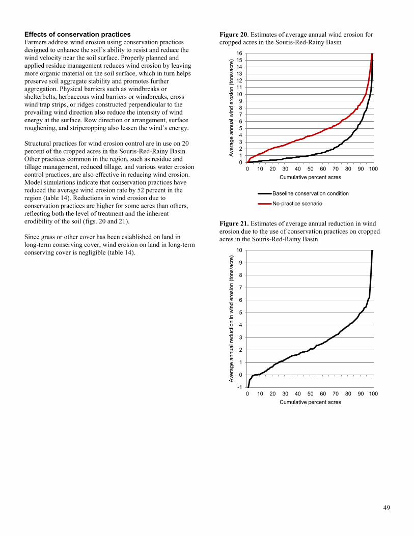
Effects of conservation practices Farmers address wind erosion using conservation practices designed to enhance the soil’s ability to resist and reduce the wind velocity near the soil surface. Properly planned and applied residue management reduces wind erosion by leaving more organic material on the soil surface, which in turn helps preserve soil aggregate stability and promotes further aggregation. Physical barriers such as windbreaks or shelterbelts, herbaceous wind barriers or windbreaks, cross wind trap strips, or ridges constructed perpendicular to the prevailing wind direction also reduce the intensity of wind energy at the surface. Row direction or arrangement, surface roughening, and stripcropping also lessen the wind’s energy. Structural practices for wind erosion control are in use on 20 percent of the cropped acres in the Souris-Red-Rainy Basin. Other practices common in the region, such as residue and tillage management, reduced tillage, and various water erosion control practices, are also effective in reducing wind erosion. Model simulations indicate that conservation practices have reduced the average wind erosion rate by 52 percent in the region (table 14). Reductions in wind erosion due to conservation practices are higher for some acres than others, reflecting both the level of treatment and the inherent erodibility of the soil (figs. 20 and 21). Since grass or other cover has been established on land in long-term conserving cover, wind erosion on land in long-term conserving cover is negligible (table 14).

Figure 20. Estimates of average annual wind erosion for cropped acres in the Souris-Red-Rainy Basin

Figure 21. Estimates of average annual reduction in wind erosion due to the use of conservation practices on cropped acres in the Souris-Red-Rainy Basin

0123456789

10111213141516

0 10 20 30 40 50 60 70 80 90 100

Ave

rage

ann

ual w

ind

eros

ion

(tons

/acr

e)

Cumulative percent acres

Baseline conservation condition

No-practice scenario

-1

0

1

2

3

4

5

6

7

8

9

10

0 10 20 30 40 50 60 70 80 90 100

Ave

rage

ann

ual r

educ

tion

in w

ind

eros

ion

(tons

/acr

e)

Cumulative percent acres

49

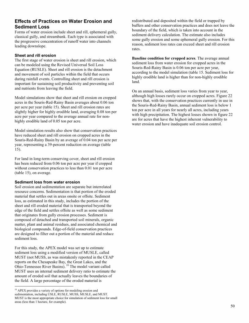
Effects of Practices on Water Erosion and Sediment Loss Forms of water erosion include sheet and rill, ephemeral gully, classical gully, and streambank. Each type is associated with the progressive concentration of runoff water into channels leading downslope. Sheet and rill erosion The first stage of water erosion is sheet and rill erosion, which can be modeled using the Revised Universal Soil Loss Equation (RUSLE). Sheet and rill erosion is the detachment and movement of soil particles within the field that occurs during rainfall events. Controlling sheet and rill erosion is important for sustaining soil productivity and preventing soil and nutrients from leaving the field. Model simulations show that sheet and rill erosion on cropped acres in the Souris-Red-Rainy Basin averages about 0.06 ton per acre per year (table 15). Sheet and rill erosion rates are slightly higher for highly erodible land, averaging 0.08 ton per acre per year compared to the average annual rate for non-highly erodible land of 0.05 ton per acre. Model simulation results also show that conservation practices have reduced sheet and rill erosion on cropped acres in the Souris-Red-Rainy Basin by an average of 0.04 ton per acre per year, representing a 39-percent reduction on average (table 15). For land in long-term conserving cover, sheet and rill erosion has been reduced from 0.06 ton per acre per year if cropped without conservation practices to less than 0.01 ton per acre (table 15), on average. Sediment loss from water erosion Soil erosion and sedimentation are separate but interrelated resource concerns. Sedimentation is that portion of the eroded material that settles out in areas onsite or offsite. Sediment loss, as estimated in this study, includes the portion of the sheet and rill eroded material that is transported beyond the edge of the field and settles offsite as well as some sediment that originates from gully erosion processes. Sediment is composed of detached and transported soil minerals, organic matter, plant and animal residues, and associated chemical and biological compounds. Edge-of-field conservation practices are designed to filter out a portion of the material and reduce sediment loss. For this study, the APEX model was set up to estimate sediment loss using a modified version of MUSLE, called MUST (not MUSS, as was mistakenly reported in the CEAP reports on the Chesapeake Bay, the Great Lakes, and the Ohio-Tennessee River Basins).17F

18 The model variant called MUST uses an internal sediment delivery ratio to estimate the amount of eroded soil that actually leaves the boundaries of the field. A large percentage of the eroded material is

18 APEX provides a variety of options for modeling erosion and sedimentation, including USLE, RUSLE, MUSS, MUSLE, and MUST. MUST is the most appropriate choice for simulation of sediment loss for small areas (less than 1 hectare, for example).

redistributed and deposited within the field or trapped by buffers and other conservation practices and does not leave the boundary of the field, which is taken into account in the sediment delivery calculation. The estimate also includes some gully erosion and some ephemeral gully erosion. For this reason, sediment loss rates can exceed sheet and rill erosion rates. Baseline condition for cropped acres. The average annual sediment loss from water erosion for cropped acres in the Souris-Red-Rainy Basin is 0.06 ton per acre per year, according to the model simulation (table 15. Sediment loss for highly erodible land is higher than for non-highly erodible land. On an annual basis, sediment loss varies from year to year, although high losses rarely occur on cropped acres. Figure 22 shows that, with the conservation practices currently in use in the Souris-Red-Rainy Basin, annual sediment loss is below 1 ton per acre in all years for nearly all acres, including years with high precipitation. The highest losses shown in figure 22 are for acres that have the highest inherent vulnerability to water erosion and have inadequate soil erosion control.

50

Table 15. Field-level effects of conservation practices on erosion and sediment loss for cultivated cropland in the Souris-Red-Rainy Basin

Model simulated outcome

Baseline conservation

condition

No-practice scenario

Reduction due to practices

Percent reduction

Cropped acres (17.6 million acres) Average annual sheet and rill erosion (tons/acre)* 0.06 0.09 0.04 39 Average annual sediment loss at edge of field due to water erosion (tons/acre)** 0.06 0.11 0.05 43

Highly erodible land (13 percent of cropped acres) Average annual sheet and rill erosion (tons/acre)* 0.08 0.14 0.06 41 Average annual sediment loss at edge of field due to water erosion (tons/acre)** 0.11 0.17 0.06 36

Non-highly erodible land (87 percent of cropped acres) Average annual sheet and rill erosion (tons/acre)* 0.05 0.08 0.03 38 Average annual sediment loss at edge of field due to water erosion (tons/acre)** 0.06 0.10 0.05 45

Land in long-term conserving cover (2.3 million acres) Average annual sheet and rill erosion (tons/acre)* <0.01 0.06 0.06 100 Average annual sediment loss at edge of field due to water erosion (tons/acre) <0.01 0.09 0.09 99

* Estimated using the Revised Universal Soil Loss Equation. **Estimated using MUST, which includes some sediment from gully erosion. See text. Note: Percent reductions were calculated prior to rounding the values for reporting in the table and the associated text. Note: Model simulation results for the baseline conservation condition are presented in appendix B for subregions 0901 and 0902. Figure 22. Distribution of annual sediment loss for each year of the 47-year model simulation, Souris-Red-Rainy Basin

Note: This figure shows how annual sediment loss (tons per acre per year) varies within the region and from year to year in the model simulation for cropped acres. Each of the 47 curves shown above represents a single year of data and shows how annual sediment loss varies over the region in that year, starting with the acres with the lowest sediment loss and increasing to the acres with the highest sediment loss. The family of curves shows how annual sediment loss varies from year to year.

0.0

0.5

1.0

1.5

2.0

2.5

3.0

0 10 20 30 40 50 60 70 80 90 100

Ann

ual s

edim

ent l

oss

(tons

/acr

e)

Cumulative percent acres

51

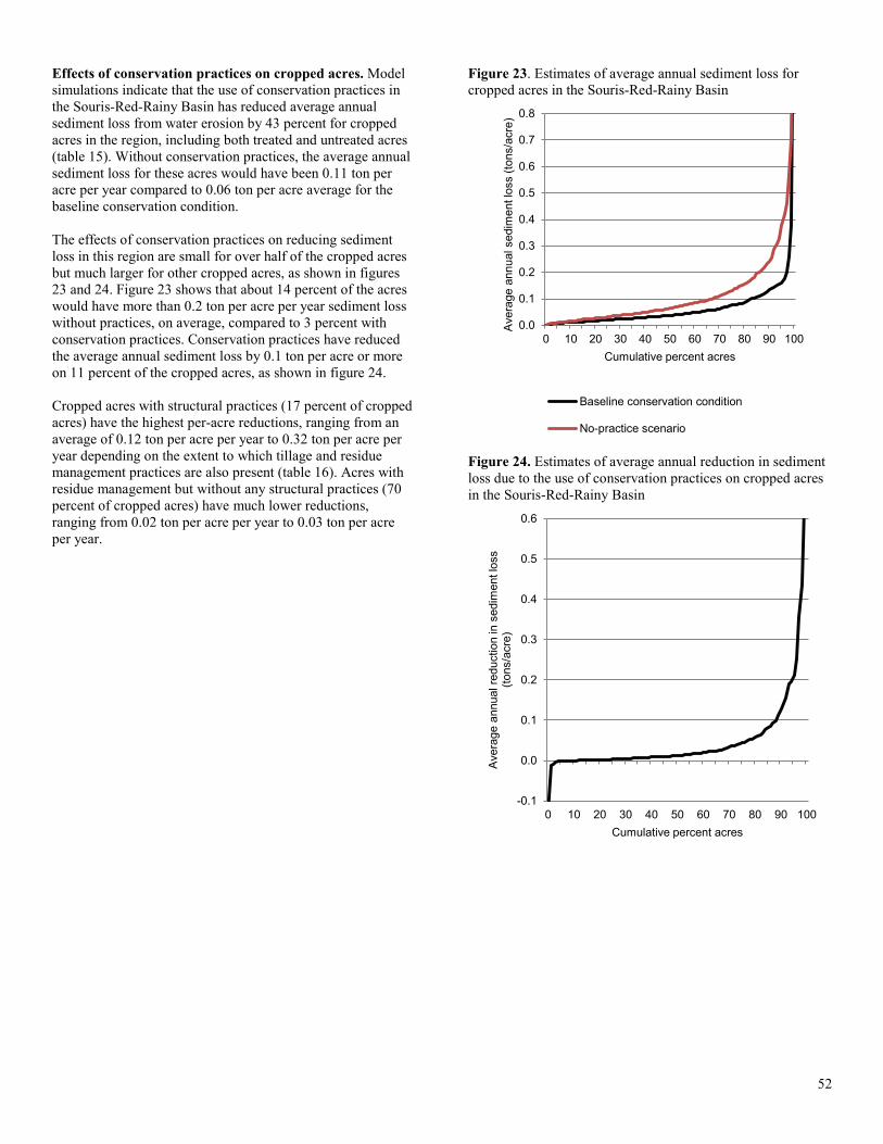
Effects of conservation practices on cropped acres. Model simulations indicate that the use of conservation practices in the Souris-Red-Rainy Basin has reduced average annual sediment loss from water erosion by 43 percent for cropped acres in the region, including both treated and untreated acres (table 15). Without conservation practices, the average annual sediment loss for these acres would have been 0.11 ton per acre per year compared to 0.06 ton per acre average for the baseline conservation condition. The effects of conservation practices on reducing sediment loss in this region are small for over half of the cropped acres but much larger for other cropped acres, as shown in figures 23 and 24. Figure 23 shows that about 14 percent of the acres would have more than 0.2 ton per acre per year sediment loss without practices, on average, compared to 3 percent with conservation practices. Conservation practices have reduced the average annual sediment loss by 0.1 ton per acre or more on 11 percent of the cropped acres, as shown in figure 24. Cropped acres with structural practices (17 percent of cropped acres) have the highest per-acre reductions, ranging from an average of 0.12 ton per acre per year to 0.32 ton per acre per year depending on the extent to which tillage and residue management practices are also present (table 16). Acres with residue management but without any structural practices (70 percent of cropped acres) have much lower reductions, ranging from 0.02 ton per acre per year to 0.03 ton per acre per year.

Figure 23. Estimates of average annual sediment loss for cropped acres in the Souris-Red-Rainy Basin

Figure 24. Estimates of average annual reduction in sediment loss due to the use of conservation practices on cropped acres in the Souris-Red-Rainy Basin

0.0

0.1

0.2

0.3

0.4

0.5

0.6

0.7

0.8

0 10 20 30 40 50 60 70 80 90 100

Ave

rage

ann

ual s

edim

ent l

oss

(tons

/acr

e)

Cumulative percent acres

Baseline conservation condition

No-practice scenario

-0.1

0.0

0.1

0.2

0.3

0.4

0.5

0.6

0 10 20 30 40 50 60 70 80 90 100

Ave

rage

ann

ual r

educ

tion

in s

edim

ent l

oss

(tons

/acr

e)

Cumulative percent acres

52

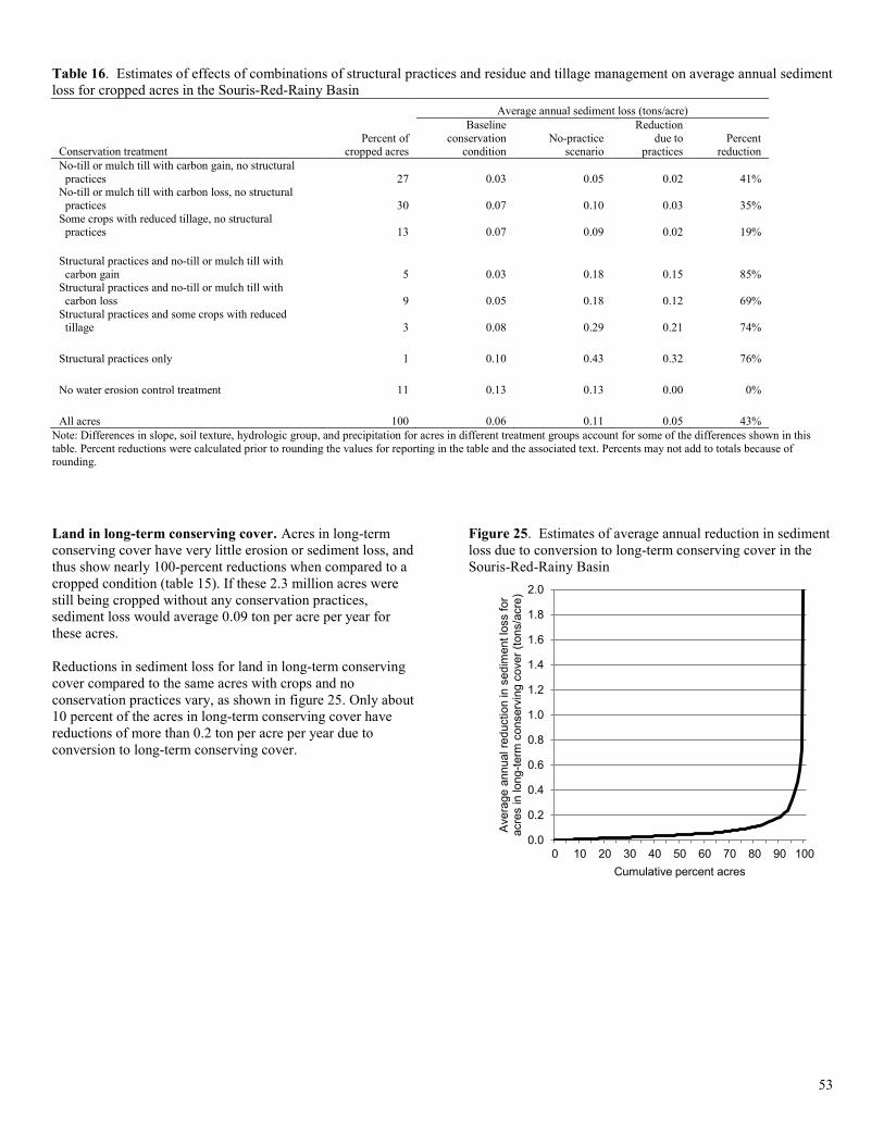
Table 16. Estimates of effects of combinations of structural practices and residue and tillage management on average annual sediment loss for cropped acres in the Souris-Red-Rainy Basin

Average annual sediment loss (tons/acre)

Conservation treatment Percent of

cropped acres

Baseline conservation

condition No-practice

scenario

Reduction due to

practices Percent

reduction No-till or mulch till with carbon gain, no structural

practices 27 0.03 0.05 0.02 41% No-till or mulch till with carbon loss, no structural

practices 30 0.07 0.10 0.03 35% Some crops with reduced tillage, no structural

practices 13 0.07 0.09 0.02 19% Structural practices and no-till or mulch till with

carbon gain 5 0.03 0.18 0.15 85% Structural practices and no-till or mulch till with

carbon loss 9 0.05 0.18 0.12 69% Structural practices and some crops with reduced

tillage 3 0.08 0.29 0.21 74% Structural practices only 1 0.10 0.43 0.32 76% No water erosion control treatment 11 0.13 0.13 0.00 0% All acres 100 0.06 0.11 0.05 43%

Note: Differences in slope, soil texture, hydrologic group, and precipitation for acres in different treatment groups account for some of the differences shown in this table. Percent reductions were calculated prior to rounding the values for reporting in the table and the associated text. Percents may not add to totals because of rounding. Land in long-term conserving cover. Acres in long-term conserving cover have very little erosion or sediment loss, and thus show nearly 100-percent reductions when compared to a cropped condition (table 15). If these 2.3 million acres were still being cropped without any conservation practices, sediment loss would average 0.09 ton per acre per year for these acres. Reductions in sediment loss for land in long-term conserving cover compared to the same acres with crops and no conservation practices vary, as shown in figure 25. Only about 10 percent of the acres in long-term conserving cover have reductions of more than 0.2 ton per acre per year due to conversion to long-term conserving cover.

Figure 25. Estimates of average annual reduction in sediment loss due to conversion to long-term conserving cover in the Souris-Red-Rainy Basin

0.0

0.2

0.4

0.6

0.8

1.0

1.2

1.4

1.6

1.8

2.0

0 10 20 30 40 50 60 70 80 90 100

Ave

rage

ann

ual r

educ

tion

in s

edim

ent l

oss

for

acre

s in

long

-term

con

serv

ing

cove

r (to

ns/a

cre)

Cumulative percent acres

53

Effects of Practices on Soil Organic Carbon Cropland acres in the Souris-Red-Rainy Basin have been smoothed by glaciation, and soils formed from glacial till and lacustrine deposits from ancient glacial lakes. These are fertile soils on gently sloping landscape but agricultural productivity can be limited by precipitation and short growing season. The colder climate of this region is conducive to preserving organic material by slowing the degradation processes. Inherent carbon accumulation in soils is a product of this colder climate and thousands of years of grassland vegetation that emerged post-glaciation. Many of the soils, particularly in the Red River Valley, are poorly drained. This restricted natural drainage also benefits soil carbon accumulation. In some areas, salinity can be a concern in the more poorly drained soils, which is a detriment to carbon sequestration. The accumulation of soil organic carbon is a balance of moisture, temperature, and soil erodibility with crop residue production, tillage, and erosion control practices. Crop production practices tend to override any beneficial effects of climate for carbon sequestration and exacerbate carbon losses in less favorable climates. Approximately 23 percent of cropped acres have a crop rotation with low residue crops like continuous soybeans, vegetables, potatoes, and sugarbeets. These crops also tend to utilize more intense tillage methods and therefore make it very difficult for increases in carbon stores even when combined with higher residue crops. The remaining 77 percent of acres have at least one high residue crop in rotation such as corn, wheat, and/or other close grown crop that produces significant stover available for improving carbon stores. Nearly 33 percent of cropped acres had a high or moderately high level for residue and tillage management with annual average gains in soil organic carbon (fig. 8). The majority of cropped acres (58 percent) had a moderate level of residue and tillage management indicating an imbalance between tillage and crop residue production and protection. Periodic increases in tillage for one or more crops in the rotation may also be reducing the acres gaining soil organic carbon by cancelling the gains of conservation tillage and/or high residue crops in rotation. In this study, estimation of soil organic carbon change is based on beginning soil characteristics that reflect the effects of years of traditional conventional tillage practices and older, lower-yielding crop varieties. These effects generally resulted in soils with organic carbon levels at or near their low steady state. Modern high-yielding crop varieties with and without the adoption of conservation tillage tend to readily improve the status of carbon in many soils, especially those with beginning stocks far less than the steady state representation of the present management. Beginning the simulations at a lower steady state for carbon allows for a more equitable comparison of conservation practices, particularly conservation tillage.

Because of this, however, model estimates of soil organic carbon change may be somewhat larger than shown in other studies. Nevertheless, model estimates obtained in this study fall within the expected range for the continuum of adoption of new crop genetics and tillage practices. Baseline condition for cropped acres Model simulation shows that for the baseline conservation condition the average annual soil organic carbon change is a loss of 69 pounds per acre per year, on average (table 17). Thirty-seven percent of cropped acres are gaining soil organic carbon (fig. 26) at an average rate of 64 pounds per acre per year. In contrast, 63 percent of cropped acres are losing soil organic carbon at an average rate of 148 pounds per acre per year. These estimates account for losses of carbon with sediment removed from the field by wind and water erosion. Loss of soil organic carbon due to wind and water erosion averages about 168 pounds per acre per year for the baseline conservation condition (table 17). Such losses are partially offset by gains in soil organic carbon due to incorporation of crop residues. Cropped acres that are gaining soil organic carbon every year provide soil quality benefits that enhance production and reduce the potential for sediment, nutrient, and pesticide losses. Soil organic carbon improves the soil’s ability to function with respect to nutrient cycling, improves water holding capacity, and reduces erodibility through enhanced soil aggregate stability. Cropping systems can be considered to be maintaining soil organic carbon if average annual losses do not exceed 100 pounds per acre per year; this rate of change is typically too small to detect via typical soil sampling over a 20-year period. Applying this criterion, about 29 percent of cropped acres in the region would be considered to be maintaining—but not enhancing—soil organic carbon (fig. 26). When combined with acres enhancing soil organic carbon, a total of 66 percent of the acres in the region are either maintaining or enhancing soil organic carbon.

54

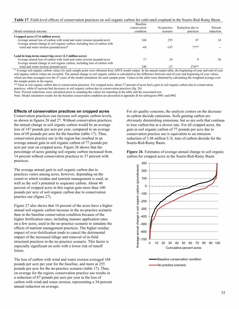
Table 17. Field-level effects of conservation practices on soil organic carbon for cultivated cropland in the Souris-Red-Rainy Basin

Model simulated outcome

Baseline conservation

condition No-practice

scenario Reduction due to

practices Percent

reduction

Cropped acres (17.6 million acres) Average annual loss of carbon with wind and water erosion (pounds/acre) 168 255 87 34 Average annual change in soil organic carbon, including loss of carbon with

wind and water erosion (pounds/acre)* -69 -147 77** -- Land in long-term conserving cover (2.3 million acres)

Average annual loss of carbon with wind and water erosion (pounds/acre) 17 26 9 36 Average annual change in soil organic carbon, including loss of carbon with

wind and water erosion (pounds/acre) 248 -27 274** * Average soil organic carbon values for each sample point were obtained from APEX model output. In the annual output table, the beginning-of-year and end-of-year soil organic carbon values are recorded. The annual change in soil organic carbon is calculated as the difference between end-of-year and beginning-of-year values, which are then averaged over the 47 years of the model simulation for each sample point. Values in the table were obtained by calculating the weighted average over the sample points in the region. ** Gain in soil organic carbon due to conservation practices. For cropped acres, about 37 percent of acres had a gain in soil organic carbon due to conservation practices, while 63 percent had decreases in soil organic carbon due to conservation practices (fig. 26) Note: Percent reductions were calculated prior to rounding the values for reporting in the table and the associated text. Note: Model simulation results for the baseline conservation condition are presented in appendix B for subregions 0901 and 0902 . Effects of conservation practices on cropped acres Conservation practices can increase soil organic carbon levels, as shown in figures 26 and 27. Without conservation practices, the annual change in soil organic carbon would be an average loss of 147 pounds per acre per year, compared to an average loss of 69 pounds per acre for the baseline (table 17). Thus, conservation practice use in the region has resulted in an average annual gain in soil organic carbon of 77 pounds per acre per year on cropped acres. Figure 26 shows that the percentage of acres gaining soil organic carbon increased from 14 percent without conservation practices to 37 percent with practices. The average annual gain in soil organic carbon due to practices varies among acres, however, depending on the extent to which residue and nutrient management is used, as well as the soil’s potential to sequester carbon. About 40 percent of cropped acres in this region gain more than 100 pounds per acre of soil organic carbon due to conservation practice use (figure 27). Figure 27 also shows that 16 percent of the acres have a higher annual soil organic carbon increase in the no-practice scenario than in the baseline conservation condition because of the higher fertilization rates, including manure application rates on a few acres, used in the no-practice scenario to simulate the effects of nutrient management practices. The higher residue impact of over-fertilization tends to cancel the detrimental impact of the increased tillage and removal of in-field structural practices in the no-practice scenario. This factor is especially significant on soils with a lower risk of runoff losses. The loss of carbon with wind and water erosion averaged 168 pounds per acre per year for the baseline, and more at 255 pounds per acre for the no-practice scenario (table 17). Thus, on average for the region, conservation practice use results in a reduction of 87 pounds per acre per year in the loss of carbon with wind and water erosion, representing a 34-percent annual reduction on average.

For air quality concerns, the analysis centers on the decrease in carbon dioxide emissions. Soils gaining carbon are obviously diminishing emissions, but so are soils that continue to lose carbon but at a slower rate. For all cropped acres, the gain in soil organic carbon of 77 pounds per acre due to conservation practice use is equivalent to an emission reduction of 2.48 million U.S. tons of carbon dioxide for the Souris-Red-Rainy Basin. Figure 26. Estimates of average annual change in soil organic carbon for cropped acres in the Souris-Red-Rainy Basin

-700

-600

-500

-400

-300

-200

-100

0

100

200

300

0 10 20 30 40 50 60 70 80 90 100

Ave

rage

ann

ual c

hang

e in

soi

l org

anic

car

bon

(pou

nds/

acre

)

Cumulative percent acres

Baseline conservation condition

No-practice scenario

55

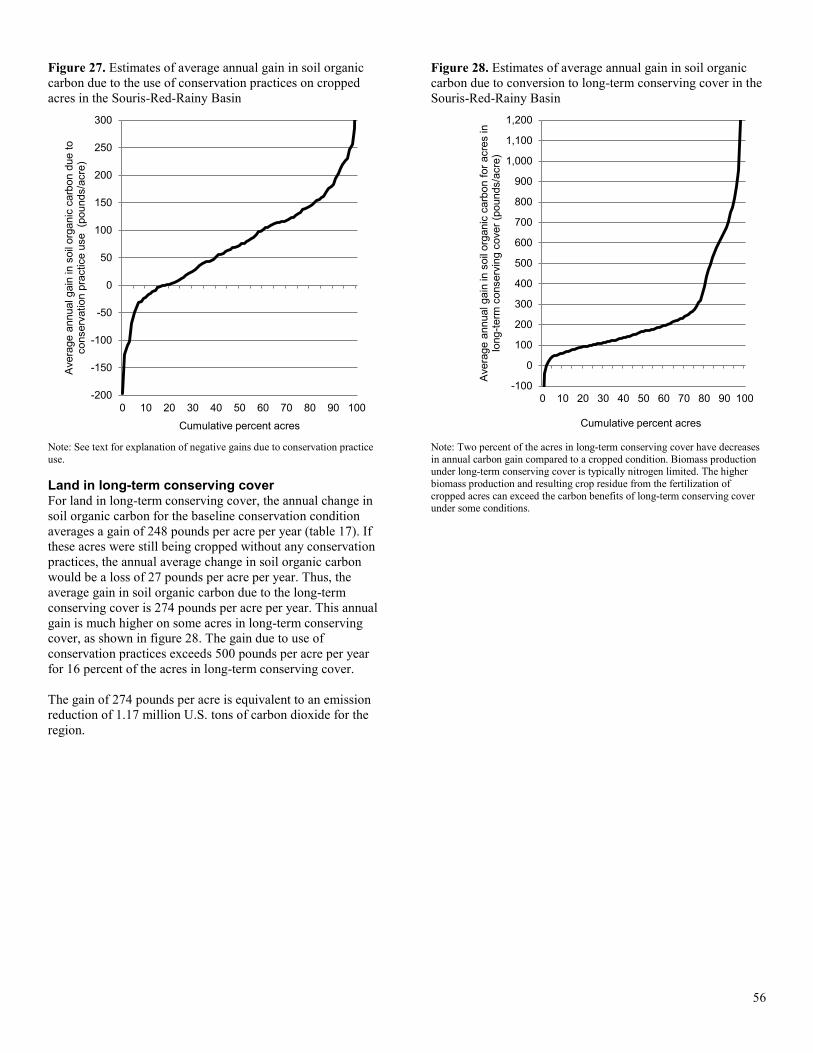
Figure 27. Estimates of average annual gain in soil organic carbon due to the use of conservation practices on cropped acres in the Souris-Red-Rainy Basin

Note: See text for explanation of negative gains due to conservation practice use. Land in long-term conserving cover For land in long-term conserving cover, the annual change in soil organic carbon for the baseline conservation condition averages a gain of 248 pounds per acre per year (table 17). If these acres were still being cropped without any conservation practices, the annual average change in soil organic carbon would be a loss of 27 pounds per acre per year. Thus, the average gain in soil organic carbon due to the long-term conserving cover is 274 pounds per acre per year. This annual gain is much higher on some acres in long-term conserving cover, as shown in figure 28. The gain due to use of conservation practices exceeds 500 pounds per acre per year for 16 percent of the acres in long-term conserving cover. The gain of 274 pounds per acre is equivalent to an emission reduction of 1.17 million U.S. tons of carbon dioxide for the region.

Figure 28. Estimates of average annual gain in soil organic carbon due to conversion to long-term conserving cover in the Souris-Red-Rainy Basin

Note: Two percent of the acres in long-term conserving cover have decreases in annual carbon gain compared to a cropped condition. Biomass production under long-term conserving cover is typically nitrogen limited. The higher biomass production and resulting crop residue from the fertilization of cropped acres can exceed the carbon benefits of long-term conserving cover under some conditions.

-200

-150

-100

-50

0

50

100

150

200

250

300

0 10 20 30 40 50 60 70 80 90 100

Ave

rage

ann

ual g

ain

in s

oil o

rgan

ic c

arbo

n du

e to

co

nser

vatio

n pr

actic

e us

e (p

ound

s/ac

re)

Cumulative percent acres

-100

0

100

200

300

400

500

600

700

800

900

1,000

1,100

1,200

0 10 20 30 40 50 60 70 80 90 100

Ave

rage

ann

ual g

ain

in s

oil o

rgan

ic c

arbo

n fo

r acr

es in

lo

ng-te

rm c

onse

rvin

g co

ver (

poun

ds/a

cre)

Cumulative percent acres

56

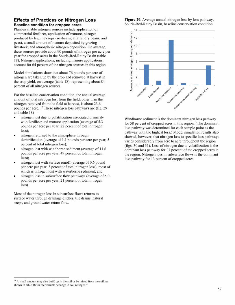
Effects of Practices on Nitrogen Loss Baseline condition for cropped acres Plant-available nitrogen sources include application of commercial fertilizer, application of manure, nitrogen produced by legume crops (soybeans, alfalfa, dry beans, and peas), a small amount of manure deposited by grazing livestock, and atmospheric nitrogen deposition. On average, these sources provide about 90 pounds of nitrogen per acre per year for cropped acres in the Souris-Red-Rainy Basin (table 18). Nitrogen applications, including manure applications, account for 64 percent of the nitrogen sources in this region. Model simulations show that about 76 pounds per acre of nitrogen are taken up by the crop and removed at harvest in the crop yield, on average (table 18), representing about 84 percent of all nitrogen sources. For the baseline conservation condition, the annual average amount of total nitrogen lost from the field, other than the nitrogen removed from the field at harvest, is about 23.6 pounds per acre. 18F

19 These nitrogen loss pathways are (fig. 29 and table 18)— • nitrogen lost due to volatilization associated primarily

with fertilizer and manure application (average of 5.3 pounds per acre per year, 22 percent of total nitrogen loss);

• nitrogen returned to the atmosphere through denitrification (average of 1.1 pounds per acre per year, 5 percent of total nitrogen loss);

• nitrogen lost with windborne sediment (average of 11.6 pounds per acre per year, 49 percent of total nitrogen loss);

• nitrogen lost with surface runoff (average of 0.6 pound per acre per year, 3 percent of total nitrogen loss), most of which is nitrogen lost with waterborne sediment; and

• nitrogen loss in subsurface flow pathways (average of 5.0 pounds per acre per year, 21 percent of total nitrogen loss).

Most of the nitrogen loss in subsurface flows returns to surface water through drainage ditches, tile drains, natural seeps, and groundwater return flow.

19 A small amount may also build up in the soil or be mined from the soil, as shown in table 18 for the variable “change in soil nitrogen.”

Figure 29. Average annual nitrogen loss by loss pathway, Souris-Red-Rainy Basin, baseline conservation condition

Windborne sediment is the dominant nitrogen loss pathway for 58 percent of cropped acres in this region. (The dominant loss pathway was determined for each sample point as the pathway with the highest loss.) Model simulation results also showed, however, that nitrogen loss to specific loss pathways varies considerably from acre to acre throughout the region (figs. 30 and 31). Loss of nitrogen due to volatilization is the dominant loss pathway for 27 percent of the cropped acres in the region. Nitrogen loss in subsurface flows is the dominant loss pathway for 13 percent of cropped acres.

0

2

4

6

8

10

12

14

Ave

rage

ann

ual n

itrog

en lo

ss (p

ound

s/ac

re)

57

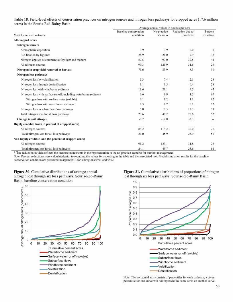
Table 18. Field-level effects of conservation practices on nitrogen sources and nitrogen loss pathways for cropped acres (17.6 million acres) in the Souris-Red-Rainy Basin Average annual values in pounds per acre

Model simulated outcome Baseline conservation

condition No-practice

scenario Reduction due to

practices Percent

reduction All cropped acres

Nitrogen sources Atmospheric deposition 3.9 3.9 0.0 0 Bio-fixation by legumes 28.9 21.0 -7.9 -38 Nitrogen applied as commercial fertilizer and manure 57.5 97.0 39.5 41 All nitrogen sources 90.3 121.9 31.6 26

Nitrogen in crop yield removed at harvest 75.6 83.9 8.3 10 Nitrogen loss pathways

Nitrogen loss by volatilization 5.3 7.4 2.1 28 Nitrogen loss through denitrification 1.1 1.5 0.4 28 Nitrogen lost with windborne sediment 11.6 21.1 9.5 45 Nitrogen loss with surface runoff, including waterborne sediment 0.6 1.9 1.3 67

Nitrogen loss with surface water (soluble) 0.1 1.2 1.1 92 Nitrogen loss with waterborne sediment 0.5 0.7 0.1 22

Nitrogen loss in subsurface flow pathways 5.0 17.3 12.3 71 Total nitrogen loss for all loss pathways 23.6 49.2 25.6 52

Change in soil nitrogen -9.7 -12.0 -2.3 -- Highly erodible land (13 percent of cropped acres)

All nitrogen sources 84.2 114.2 30.0 26 Total nitrogen loss for all loss pathways 20.0 45.9 25.9 57

Non-highly erodible land (87 percent of cropped acres) All nitrogen sources 91.2 123.1 31.8 26 Total nitrogen loss for all loss pathways 24.1 49.7 25.6 51

* The reduction in yield reflects the increase in nutrients in the representation in the no-practice scenario for nutrient management. Note: Percent reductions were calculated prior to rounding the values for reporting in the table and the associated text. Model simulation results for the baseline conservation condition are presented in appendix B for subregions 0901 and 0902. Figure 30. Cumulative distributions of average annual nitrogen lost through six loss pathways, Souris-Red-Rainy Basin, baseline conservation condition

Figure 31. Cumulative distributions of proportions of nitrogen lost through six loss pathways, Souris-Red-Rainy Basin

Note: The horizontal axis consists of percentiles for each pathway; a given percentile for one curve will not represent the same acres on another curve.

0

10

20

30

40

50

60

0 10 20 30 40 50 60 70 80 90 100

Ave

rage

ann

ual n

itrog

en lo

ss (p

ound

s/ac

re)

Cumulative percent acres Waterborne sedimentSurface water runoff (soluble)Subsurface flowsWindborne sedimentVolatilizationDenitrification

0.0

0.1

0.2

0.3

0.4

0.5

0.6

0.7

0.8

0.9

1.0

0 10 20 30 40 50 60 70 80 90 100

Pro

porti

on o

f nitr

ogen

loss

Cumulative percent acres

Waterborne sedimentSurface water runoff (soluble)Subsurface flowsWindborne sedimentVolatilizationDenitrification

58

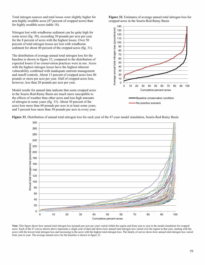
Total nitrogen sources and total losses were slightly higher for non-highly erodible acres (87 percent of cropped acres) than for highly erodible acres (table 18). Nitrogen lost with windborne sediment can be quite high for some acres (fig. 30), exceeding 30 pounds per acre per year for the 8 percent of acres with the highest losses. Over 50 percent of total nitrogen losses are lost with windborne sediment for about 40 percent of the cropped acres (fig. 31). The distribution of average annual total nitrogen loss for the baseline is shown in figure 32, compared to the distribution of expected losses if no conservation practices were in use. Acres with the highest nitrogen losses have the highest inherent vulnerability combined with inadequate nutrient management and runoff controls. About 13 percent of cropped acres lose 40 pounds or more per acre per year. Half of cropped acres lose, however, less than 20 pounds per acre per year. Model results for annual data indicate that some cropped acres in the Souris-Red-Rainy Basin are much more susceptible to the effects of weather than other acres and lose high amounts of nitrogen in some years (fig. 33). About 30 percent of the acres lose more than 60 pounds per acre in at least some years, and 5 percent lose more than 30 pounds per acre in every year.

Figure 32. Estimates of average annual total nitrogen loss for cropped acres in the Souris-Red-Rainy Basin

Figure 33. Distribution of annual total nitrogen loss for each year of the 47-year model simulation, Souris-Red-Rainy Basin

Note: This figure shows how annual total nitrogen loss (pounds per acre per year) varied within the region and from year to year in the model simulation for cropped acres. Each of the 47 curves shown above represents a single year of data and shows how annual total nitrogen loss varied over the region in that year, starting with the acres with the lowest total nitrogen loss and increasing to the acres with the highest total nitrogen loss. The family of curves shows how annual total nitrogen loss varied from year to year. The average annual curve for the baseline is shown in figure 32.

0102030405060708090

100110120130140

0 10 20 30 40 50 60 70 80 90 100Ave

rage

ann

ual t

otal

nitr

ogen

loss

(pou

nds/

acre

)

Cumulative percent acres

Baseline conservation condition

No-practice scenario

0

20

40

60

80

100

120

140

160

180

200

220

240

260

280

300

0 10 20 30 40 50 60 70 80 90 100

Ann

ual t

otal

nitr

ogen

loss

(pou

nds/

acre

)

Cumulative percent acres

59

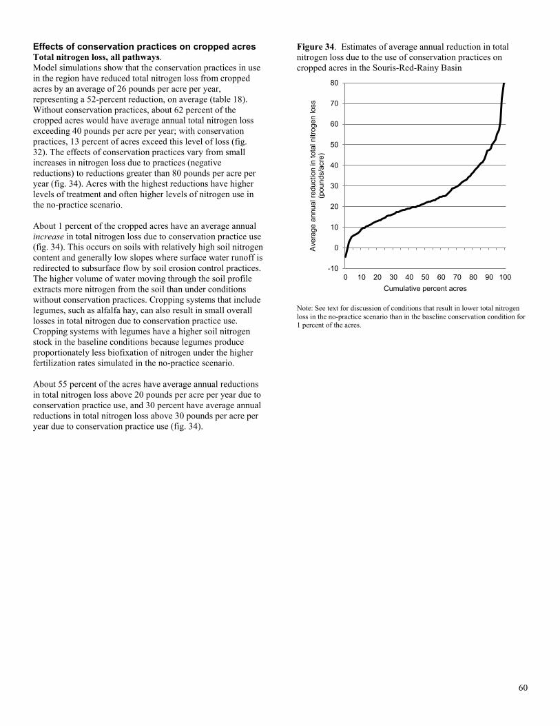
Effects of conservation practices on cropped acres Total nitrogen loss, all pathways. Model simulations show that the conservation practices in use in the region have reduced total nitrogen loss from cropped acres by an average of 26 pounds per acre per year, representing a 52-percent reduction, on average (table 18). Without conservation practices, about 62 percent of the cropped acres would have average annual total nitrogen loss exceeding 40 pounds per acre per year; with conservation practices, 13 percent of acres exceed this level of loss (fig. 32). The effects of conservation practices vary from small increases in nitrogen loss due to practices (negative reductions) to reductions greater than 80 pounds per acre per year (fig. 34). Acres with the highest reductions have higher levels of treatment and often higher levels of nitrogen use in the no-practice scenario. About 1 percent of the cropped acres have an average annual increase in total nitrogen loss due to conservation practice use (fig. 34). This occurs on soils with relatively high soil nitrogen content and generally low slopes where surface water runoff is redirected to subsurface flow by soil erosion control practices. The higher volume of water moving through the soil profile extracts more nitrogen from the soil than under conditions without conservation practices. Cropping systems that include legumes, such as alfalfa hay, can also result in small overall losses in total nitrogen due to conservation practice use. Cropping systems with legumes have a higher soil nitrogen stock in the baseline conditions because legumes produce proportionately less biofixation of nitrogen under the higher fertilization rates simulated in the no-practice scenario. About 55 percent of the acres have average annual reductions in total nitrogen loss above 20 pounds per acre per year due to conservation practice use, and 30 percent have average annual reductions in total nitrogen loss above 30 pounds per acre per year due to conservation practice use (fig. 34).

Figure 34. Estimates of average annual reduction in total nitrogen loss due to the use of conservation practices on cropped acres in the Souris-Red-Rainy Basin

Note: See text for discussion of conditions that result in lower total nitrogen loss in the no-practice scenario than in the baseline conservation condition for 1 percent of the acres.

-10

0

10

20

30

40

50

60

70

80

0 10 20 30 40 50 60 70 80 90 100

Ave

rage

ann

ual r

educ

tion

in to

tal n

itrog

en lo

ss

(pou

nds/

acre

)

Cumulative percent acres

60

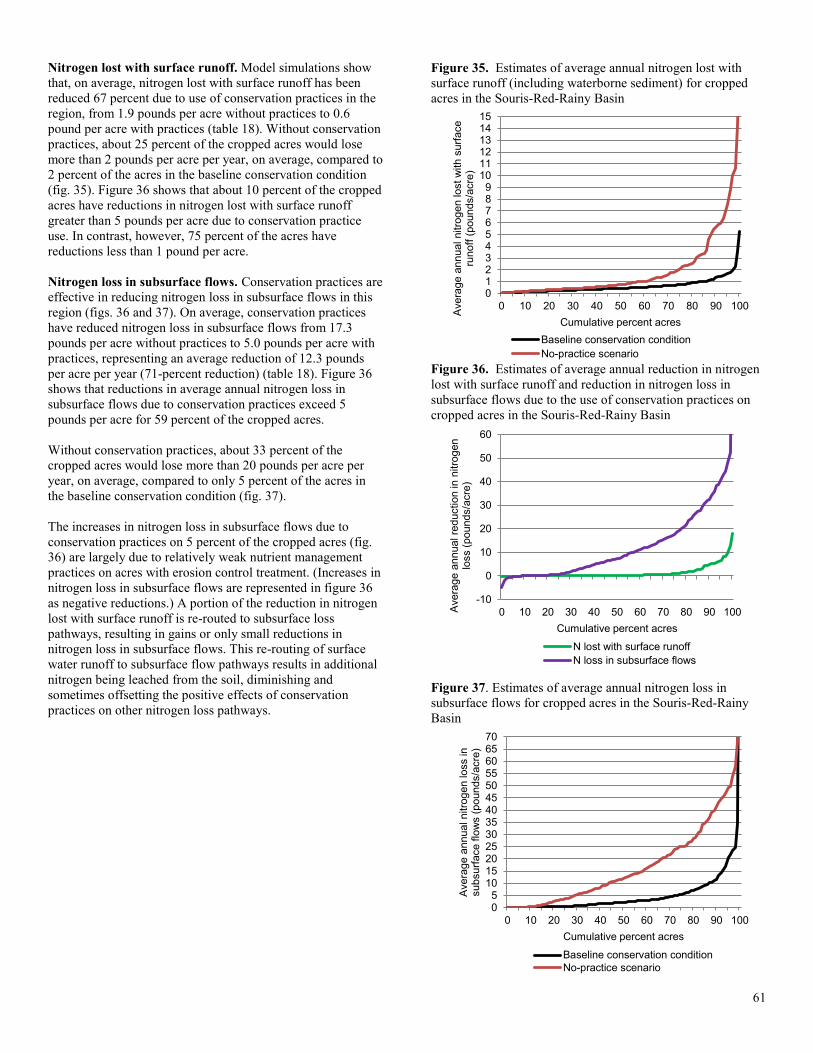
Nitrogen lost with surface runoff. Model simulations show that, on average, nitrogen lost with surface runoff has been reduced 67 percent due to use of conservation practices in the region, from 1.9 pounds per acre without practices to 0.6 pound per acre with practices (table 18). Without conservation practices, about 25 percent of the cropped acres would lose more than 2 pounds per acre per year, on average, compared to 2 percent of the acres in the baseline conservation condition (fig. 35). Figure 36 shows that about 10 percent of the cropped acres have reductions in nitrogen lost with surface runoff greater than 5 pounds per acre due to conservation practice use. In contrast, however, 75 percent of the acres have reductions less than 1 pound per acre. Nitrogen loss in subsurface flows. Conservation practices are effective in reducing nitrogen loss in subsurface flows in this region (figs. 36 and 37). On average, conservation practices have reduced nitrogen loss in subsurface flows from 17.3 pounds per acre without practices to 5.0 pounds per acre with practices, representing an average reduction of 12.3 pounds per acre per year (71-percent reduction) (table 18). Figure 36 shows that reductions in average annual nitrogen loss in subsurface flows due to conservation practices exceed 5 pounds per acre for 59 percent of the cropped acres. Without conservation practices, about 33 percent of the cropped acres would lose more than 20 pounds per acre per year, on average, compared to only 5 percent of the acres in the baseline conservation condition (fig. 37). The increases in nitrogen loss in subsurface flows due to conservation practices on 5 percent of the cropped acres (fig. 36) are largely due to relatively weak nutrient management practices on acres with erosion control treatment. (Increases in nitrogen loss in subsurface flows are represented in figure 36 as negative reductions.) A portion of the reduction in nitrogen lost with surface runoff is re-routed to subsurface loss pathways, resulting in gains or only small reductions in nitrogen loss in subsurface flows. This re-routing of surface water runoff to subsurface flow pathways results in additional nitrogen being leached from the soil, diminishing and sometimes offsetting the positive effects of conservation practices on other nitrogen loss pathways.

Figure 35. Estimates of average annual nitrogen lost with surface runoff (including waterborne sediment) for cropped acres in the Souris-Red-Rainy Basin

Figure 36. Estimates of average annual reduction in nitrogen lost with surface runoff and reduction in nitrogen loss in subsurface flows due to the use of conservation practices on cropped acres in the Souris-Red-Rainy Basin

Figure 37. Estimates of average annual nitrogen loss in subsurface flows for cropped acres in the Souris-Red-Rainy Basin

0123456789

101112131415

0 10 20 30 40 50 60 70 80 90 100Ave

rage

ann

ual n

itrog

en lo

st w

ith s

urfa

ce

runo

ff (p

ound

s/ac

re)

Cumulative percent acres Baseline conservation conditionNo-practice scenario

-10

0

10

20

30

40

50

60

0 10 20 30 40 50 60 70 80 90 100Ave

rage

ann

ual r

educ

tion

in n

itrog

en

loss

(pou

nds/

acre

)

Cumulative percent acres

N lost with surface runoffN loss in subsurface flows

05

10152025303540455055606570

0 10 20 30 40 50 60 70 80 90 100

Ave

rage

ann

ual n

itrog

en lo

ss in

su

bsur

face

flow

s (p

ound

s/ac

re)

Cumulative percent acres

Baseline conservation conditionNo-practice scenario

61

Tradeoffs in Conservation Treatment

Conservation practices applied on cropland are, for the most part, synergistic. The benefits accumulate as more practices are added to the designed systems. However, when only a single resource concern is addressed (such as soil erosion), antagonism between the practices and other resource concerns may occur. That is why it is essential that all resource concerns be considered during the conservation planning process. Most of the time the tradeoffs are much smaller than the magnitude of the primary resource concerns. Common examples are: • Terraces and conservation tillage are planned to solve a serious water erosion problem.

However, in some areas there may be concern about seeps at the lower part of the field. The planned practices will solve the erosion problem, but could exacerbate the seep problem under some conditions. Ignoring that fact does not make for an adequate conservation plan.

• Conservation tillage is planned for erosion control on a cropland field with a high water table. The reduction in runoff may increase leaching of nitrates into the shallow water table. This potential secondary problem requires additional nutrient management practices to address the concern.

• Implementation of a nutrient management plan may reduce the amount of manure added to a field and thus reduce the loss of nutrients to surface or groundwater. However, this reduction in organic material added to the field may also reduce the soil organic matter or reduce the rate of change in soil organic matter.

• Figure 34 shows that about 1 percent of the acres have an increase in total nitrogen loss due to conservation practice use in the Souris-Red-Rainy Basin. This result occurs primarily on soils with relatively high soil nitrogen content and generally low slopes where the surface water runoff is re-directed to subsurface flow by soil erosion control practices. The higher volume of water moving through the soil profile extracts more nitrogen from the soil than under conditions without conservation practices. For these fields, the nutrient management component of a farmer’s conservation plan would need to be enhanced to reduce or eliminate the negative effects of soil erosion control practices on nitrogen loss.

A comprehensive planning process is used to identify the appropriate combination of practices needed to address multiple resource concerns by taking into account the specific inherent vulnerabilities associated with each field. To ensure that proper consideration is given to the effects of conservation practices on all of the resource concerns, USDA/NRCS developed a comprehensive planning tool referred to as CPPE (Conservation Practice Physical Effects). The CPPE is included in the Field Office Technical Guide. Conservation planners are expected to use CPPE as a reference to ensure that all resource concerns are addressed in conservation plans.

62

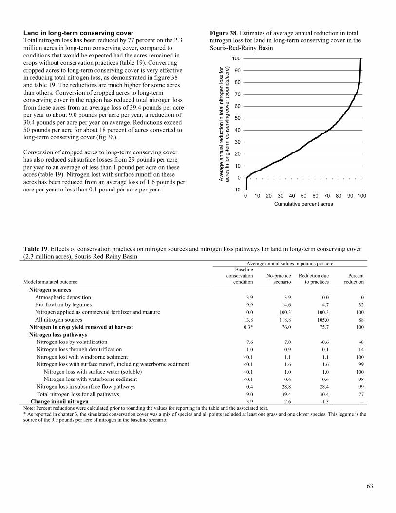
Land in long-term conserving cover Total nitrogen loss has been reduced by 77 percent on the 2.3 million acres in long-term conserving cover, compared to conditions that would be expected had the acres remained in crops without conservation practices (table 19). Converting cropped acres to long-term conserving cover is very effective in reducing total nitrogen loss, as demonstrated in figure 38 and table 19. The reductions are much higher for some acres than others. Conversion of cropped acres to long-term conserving cover in the region has reduced total nitrogen loss from these acres from an average loss of 39.4 pounds per acre per year to about 9.0 pounds per acre per year, a reduction of 30.4 pounds per acre per year on average. Reductions exceed 50 pounds per acre for about 18 percent of acres converted to long-term conserving cover (fig 38). Conversion of cropped acres to long-term conserving cover has also reduced subsurface losses from 29 pounds per acre per year to an average of less than 1 pound per acre on these acres (table 19). Nitrogen lost with surface runoff on these acres has been reduced from an average loss of 1.6 pounds per acre per year to less than 0.1 pound per acre per year.

Figure 38. Estimates of average annual reduction in total nitrogen loss for land in long-term conserving cover in the Souris-Red-Rainy Basin

Table 19. Effects of conservation practices on nitrogen sources and nitrogen loss pathways for land in long-term conserving cover (2.3 million acres), Souris-Red-Rainy Basin Average annual values in pounds per acre

Model simulated outcome

Baseline conservation

condition No-practice

scenario Reduction due

to practices Percent

reduction Nitrogen sources

Atmospheric deposition 3.9 3.9 0.0 0 Bio-fixation by legumes 9.9 14.6 4.7 32 Nitrogen applied as commercial fertilizer and manure 0.0 100.3 100.3 100 All nitrogen sources 13.8 118.8 105.0 88

Nitrogen in crop yield removed at harvest 0.3* 76.0 75.7 100 Nitrogen loss pathways

Nitrogen loss by volatilization 7.6 7.0 -0.6 -8 Nitrogen loss through denitrification 1.0 0.9 -0.1 -14 Nitrogen lost with windborne sediment <0.1 1.1 1.1 100 Nitrogen loss with surface runoff, including waterborne sediment <0.1 1.6 1.6 99

Nitrogen loss with surface water (soluble) <0.1 1.0 1.0 100 Nitrogen loss with waterborne sediment <0.1 0.6 0.6 98

Nitrogen loss in subsurface flow pathways 0.4 28.8 28.4 99 Total nitrogen loss for all pathways 9.0 39.4 30.4 77

Change in soil nitrogen 3.9 2.6 -1.3 -- Note: Percent reductions were calculated prior to rounding the values for reporting in the table and the associated text. * As reported in chapter 3, the simulated conservation cover was a mix of species and all points included at least one grass and one clover species. This legume is the source of the 9.9 pounds per acre of nitrogen in the baseline scenario.

-10

0

10

20

30

40

50

60

70

80

90

100

0 10 20 30 40 50 60 70 80 90 100

Ave

rage

ann

ual r

educ

tion

in to

tal n

itrog

en lo

ss fo

r ac

res

in lo

ng-te

rm c

onse

rvin

g co

ver (

poun

ds/a

cre)

Cumulative percent acres

63

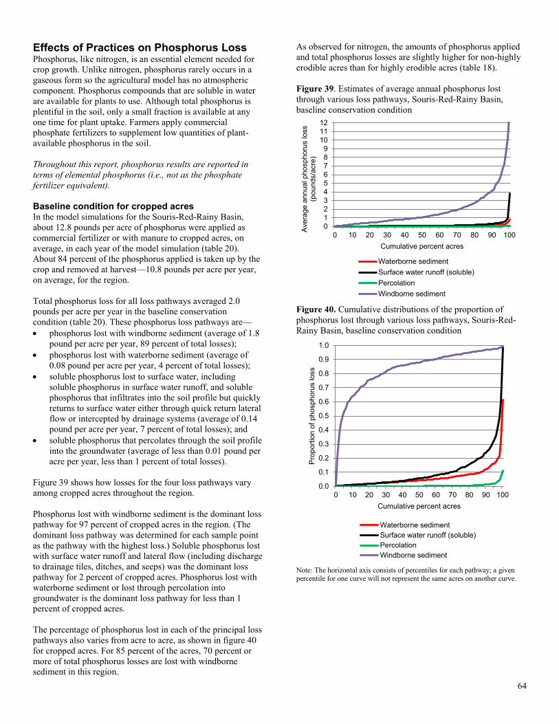
Effects of Practices on Phosphorus Loss Phosphorus, like nitrogen, is an essential element needed for crop growth. Unlike nitrogen, phosphorus rarely occurs in a gaseous form so the agricultural model has no atmospheric component. Phosphorus compounds that are soluble in water are available for plants to use. Although total phosphorus is plentiful in the soil, only a small fraction is available at any one time for plant uptake. Farmers apply commercial phosphate fertilizers to supplement low quantities of plant-available phosphorus in the soil. Throughout this report, phosphorus results are reported in terms of elemental phosphorus (i.e., not as the phosphate fertilizer equivalent). Baseline condition for cropped acres In the model simulations for the Souris-Red-Rainy Basin, about 12.8 pounds per acre of phosphorus were applied as commercial fertilizer or with manure to cropped acres, on average, in each year of the model simulation (table 20). About 84 percent of the phosphorus applied is taken up by the crop and removed at harvest—10.8 pounds per acre per year, on average, for the region. Total phosphorus loss for all loss pathways averaged 2.0 pounds per acre per year in the baseline conservation condition (table 20). These phosphorus loss pathways are— • phosphorus lost with windborne sediment (average of 1.8

pound per acre per year, 89 percent of total losses); • phosphorus lost with waterborne sediment (average of

0.08 pound per acre per year, 4 percent of total losses); • soluble phosphorus lost to surface water, including

soluble phosphorus in surface water runoff, and soluble phosphorus that infiltrates into the soil profile but quickly returns to surface water either through quick return lateral flow or intercepted by drainage systems (average of 0.14 pound per acre per year, 7 percent of total losses); and

• soluble phosphorus that percolates through the soil profile into the groundwater (average of less than 0.01 pound per acre per year, less than 1 percent of total losses).

Figure 39 shows how losses for the four loss pathways vary among cropped acres throughout the region. Phosphorus lost with windborne sediment is the dominant loss pathway for 97 percent of cropped acres in the region. (The dominant loss pathway was determined for each sample point as the pathway with the highest loss.) Soluble phosphorus lost with surface water runoff and lateral flow (including discharge to drainage tiles, ditches, and seeps) was the dominant loss pathway for 2 percent of cropped acres. Phosphorus lost with waterborne sediment or lost through percolation into groundwater is the dominant loss pathway for less than 1 percent of cropped acres. The percentage of phosphorus lost in each of the principal loss pathways also varies from acre to acre, as shown in figure 40 for cropped acres. For 85 percent of the acres, 70 percent or more of total phosphorus losses are lost with windborne sediment in this region.

As observed for nitrogen, the amounts of phosphorus applied and total phosphorus losses are slightly higher for non-highly erodible acres than for highly erodible acres (table 18). Figure 39. Estimates of average annual phosphorus lost through various loss pathways, Souris-Red-Rainy Basin, baseline conservation condition

Figure 40. Cumulative distributions of the proportion of phosphorus lost through various loss pathways, Souris-Red-Rainy Basin, baseline conservation condition

Note: The horizontal axis consists of percentiles for each pathway; a given percentile for one curve will not represent the same acres on another curve.

0123456789

101112

0 10 20 30 40 50 60 70 80 90 100

Ave

rage

ann

ual p

hosp

horu

s lo

ss

(pou

nds/

acre

)

Cumulative percent acres

Waterborne sedimentSurface water runoff (soluble)PercolationWindborne sediment

0.0

0.1

0.2

0.3

0.4

0.5

0.6

0.7

0.8

0.9

1.0

0 10 20 30 40 50 60 70 80 90 100

Pro

porti

on o

f pho

spho

rus

loss

Cumulative percent acres

Waterborne sedimentSurface water runoff (soluble)PercolationWindborne sediment

64

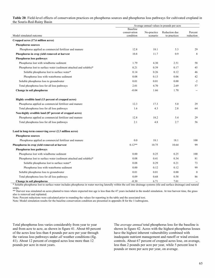
Table 20. Field-level effects of conservation practices on phosphorus sources and phosphorus loss pathways for cultivated cropland in the Souris-Red-Rainy Basin Average annual values in pounds per acre

Model simulated outcome

Baseline conservation

condition No-practice

scenario Reduction due

to practices Percent

reduction

Cropped acres (17.6 million acres) Phosphorus sources

Phosphorus applied as commercial fertilizer and manure 12.8 18.1 5.3 29 Phosphorus in crop yield removed at harvest 10.8 11.7 0.9 8 Phosphorus loss pathways

Phosphorus lost with windborne sediment 1.79 4.30 2.51 58 Phosphorus lost to surface water (sediment attached and soluble)* 0.21 0.39 0.17 45

Soluble phosphorus lost to surface water* 0.14 0.26 0.12 46 Phosphorus loss with waterborne sediment 0.08 0.13 0.06 42

Soluble phosphorus loss to groundwater 0.01 0.01 0.00 -2 Total phosphorus loss for all loss pathways 2.01 4.70 2.69 57

Change in soil phosphorus -0.04 1.66 1.70 -- Highly erodible land (13 percent of cropped acres)

Phosphorus applied as commercial fertilizer and manure 12.3 17.3 5.0 29 Total phosphorus loss for all loss pathways 1.6 4.3 2.8 64

Non-highly erodible land (87 percent of cropped acres) Phosphorus applied as commercial fertilizer and manure 12.8 18.2 5.4 29 Total phosphorus loss for all loss pathways 2.1 4.8 2.7 56

Land in long-term conserving cover (2.3 million acres)

Phosphorus sources Phosphorus applied as commercial fertilizer and manure 0.0 18.1 18.1 100

Phosphorus in crop yield removed at harvest 0.12** 10.75 10.64 99 Phosphorus loss pathways

Phosphorus lost with windborne sediment 0.00 0.25 0.25 100 Phosphorus lost to surface water (sediment attached and soluble)* 0.08 0.41 0.34 81

Soluble phosphorus lost to surface water* 0.08 0.29 0.21 73 Phosphorus loss with waterborne sediment 0.00 0.12 0.12 99

Soluble phosphorus loss to groundwater 0.01 0.01 0.00 0 Total phosphorus loss for all loss pathways 0.09 0.68 0.58 86

Change in soil phosphorus -0.30 6.71 7.01 -- * Soluble phosphorus lost to surface water includes phosphorus in water moving laterally within the soil into drainage systems (tile and surface drainage) and natural seeps. ** Harvest was simulated on acres planted to trees where expected tree age is less than the 47 years included in the model simulation. At tree harvest time, the grass also is removed and replanted. Note: Percent reductions were calculated prior to rounding the values for reporting in the table and the associated text. Note: Model simulation results for the baseline conservation condition are presented in appendix B for the 11subregions. Total phosphorus loss varies considerably from year to year and from acre to acre, as shown in figure 41. About 60 percent of the acres lose less than 4 pounds per acre per year through the various loss pathways under all weather conditions (fig. 41). About 12 percent of cropped acres lose more than 12 pounds per acre in most years.

The average annual total phosphorus loss for the baseline is shown in figure 42. Acres with the highest phosphorus losses have the highest inherent vulnerability combined with inadequate nutrient management and runoff or wind erosion controls. About 67 percent of cropped acres lose, on average, less than 2 pounds per acre per year, while 5 percent lose 6 pounds or more per acre per year, on average.

65

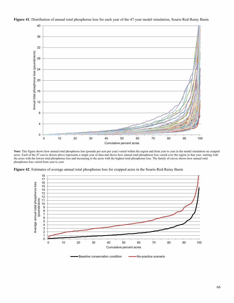
Figure 41. Distribution of annual total phosphorus loss for each year of the 47-year model simulation, Souris-Red-Rainy Basin

Note: This figure shows how annual total phosphorus loss (pounds per acre per year) varied within the region and from year to year in the model simulation on cropped acres. Each of the 47 curves shown above represents a single year of data and shows how annual total phosphorus loss varied over the region in that year, starting with the acres with the lowest total phosphorus loss and increasing to the acres with the highest total phosphorus loss. The family of curves shows how annual total phosphorus loss varied from year to year. Figure 42. Estimates of average annual total phosphorus loss for cropped acres in the Souris-Red-Rainy Basin

0

4

8

12

16

20

24

28

32

36

40

0 10 20 30 40 50 60 70 80 90 100

Ann

ual t

otal

pho

spho

rus

loss

(pou

nds/

acre

)

Cumulative percent acres

0123456789

101112131415161718

0 10 20 30 40 50 60 70 80 90 100

Ave

rage

ann

ual t

otal

pho

spho

rus

loss

(p

ound

s/ac

re)

Cumulative percent acres

Baseline conservation condition No-practice scenario

66

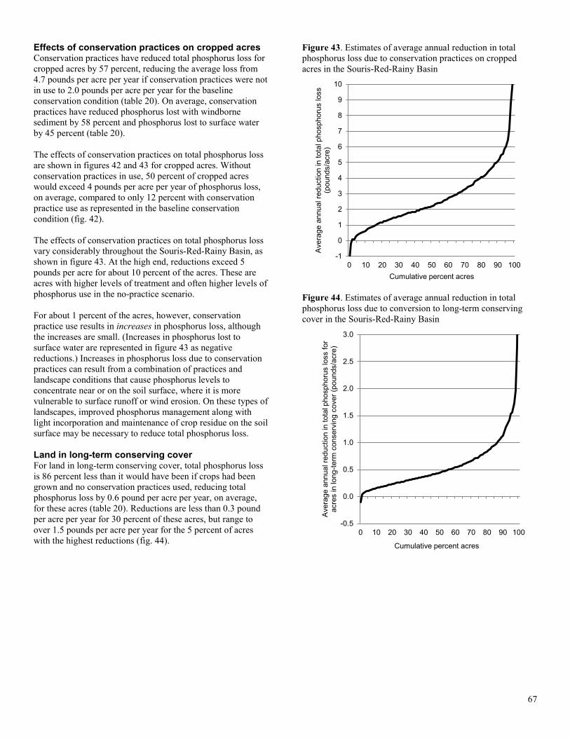
Effects of conservation practices on cropped acres Conservation practices have reduced total phosphorus loss for cropped acres by 57 percent, reducing the average loss from 4.7 pounds per acre per year if conservation practices were not in use to 2.0 pounds per acre per year for the baseline conservation condition (table 20). On average, conservation practices have reduced phosphorus lost with windborne sediment by 58 percent and phosphorus lost to surface water by 45 percent (table 20). The effects of conservation practices on total phosphorus loss are shown in figures 42 and 43 for cropped acres. Without conservation practices in use, 50 percent of cropped acres would exceed 4 pounds per acre per year of phosphorus loss, on average, compared to only 12 percent with conservation practice use as represented in the baseline conservation condition (fig. 42). The effects of conservation practices on total phosphorus loss vary considerably throughout the Souris-Red-Rainy Basin, as shown in figure 43. At the high end, reductions exceed 5 pounds per acre for about 10 percent of the acres. These are acres with higher levels of treatment and often higher levels of phosphorus use in the no-practice scenario. For about 1 percent of the acres, however, conservation practice use results in increases in phosphorus loss, although the increases are small. (Increases in phosphorus lost to surface water are represented in figure 43 as negative reductions.) Increases in phosphorus loss due to conservation practices can result from a combination of practices and landscape conditions that cause phosphorus levels to concentrate near or on the soil surface, where it is more vulnerable to surface runoff or wind erosion. On these types of landscapes, improved phosphorus management along with light incorporation and maintenance of crop residue on the soil surface may be necessary to reduce total phosphorus loss. Land in long-term conserving cover For land in long-term conserving cover, total phosphorus loss is 86 percent less than it would have been if crops had been grown and no conservation practices used, reducing total phosphorus loss by 0.6 pound per acre per year, on average, for these acres (table 20). Reductions are less than 0.3 pound per acre per year for 30 percent of these acres, but range to over 1.5 pounds per acre per year for the 5 percent of acres with the highest reductions (fig. 44).

Figure 43. Estimates of average annual reduction in total phosphorus loss due to conservation practices on cropped acres in the Souris-Red-Rainy Basin

Figure 44. Estimates of average annual reduction in total phosphorus loss due to conversion to long-term conserving cover in the Souris-Red-Rainy Basin

-1

0

1

2

3

4

5

6

7

8

9

10

0 10 20 30 40 50 60 70 80 90 100

Ave

rage

ann

ual r

educ

tion

in to

tal p

hosp

horu

s lo

ss

(pou

nds/

acre

)

Cumulative percent acres

-0.5

0.0

0.5

1.0

1.5

2.0

2.5

3.0

0 10 20 30 40 50 60 70 80 90 100

Ave

rage

ann

ual r

educ

tion

in to

tal p

hosp

horu

s lo

ss fo

r ac

res

in lo

ng-te

rm c

onse

rvin

g co

ver (

poun

ds/a

cre)

Cumulative percent acres

67

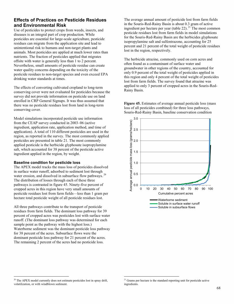
Effects of Practices on Pesticide Residues and Environmental Risk Use of pesticides to protect crops from weeds, insects, and diseases is an integral part of crop production. While pesticides are essential for large-scale agriculture, pesticide residues can migrate from the application site and lead to unintentional risk to humans and non-target plants and animals. Most pesticides are applied at much lower rates than nutrients. The fraction of pesticides applied that migrates offsite with water is generally less than 1 to 2 percent. Nevertheless, small amounts of pesticide residue can create water quality concerns depending on the toxicity of the pesticide residues to non-target species and even exceed EPA drinking water standards at times. The effects of converting cultivated cropland to long-term conserving cover were not evaluated for pesticides because the survey did not provide information on pesticide use on land enrolled in CRP General Signups. It was thus assumed that there was no pesticide residues lost from land in long-term conserving cover. Model simulations incorporated pesticide use information from the CEAP survey conducted in 2003–06 (active ingredient, application rate, application method, and time of application). A total of 110 different pesticides are used in the region, as reported in the survey. The most commonly applied pesticides are presented in table 21. The most commonly applied pesticide is the herbicide glyphosate isopropylamine salt, which accounted for 38 percent of the pesticide active ingredient applied in the region, by weight. Baseline condition for pesticide loss The APEX model tracks the mass loss of pesticides dissolved in surface water runoff, adsorbed to sediment lost through water erosion, and dissolved in subsurface flow pathways.19F

20 The distribution of losses through each of these three pathways is contrasted in figure 45. Ninety-five percent of cropped acres in this region have very small amounts of pesticide residues lost from farm fields—less than 1 gram per hectare total pesticide weight of all pesticide residues lost. All three pathways contribute to the transport of pesticide residues from farm fields. The dominant loss pathway for 39 percent of cropped acres was pesticides lost with surface water runoff. (The dominant loss pathway was determined for each sample point as the pathway with the highest loss.) Waterborne sediment was the dominant pesticide loss pathway for 38 percent of the acres. Subsurface flows were the dominant pesticide loss pathway for 21 percent of the acres. The remaining 2 percent of the acres had no pesticide loss.

20 The APEX model currently does not estimate pesticides lost in spray drift, volatilization, or with windblown sediment.

The average annual amount of pesticide lost from farm fields in the Souris-Red-Rainy Basin is about 0.3 gram of active ingredient per hectare per year (table 22).20F

21 The most common pesticide residues lost from farm fields in model simulations for the Souris-Red-Rainy Basin are the herbicides glyphosate isopropylamine salt and sulfentrazone, accounting for 25 percent and 21 percent of the total weight of pesticide residues lost in the region, respectively. The herbicide atrazine, commonly used on corn acres and often found as a contaminant of surface water and groundwater in other regions of the country, accounted for only 0.9 percent of the total weight of pesticides applied in this region and only 4 percent of the total weight of pesticides lost from farm fields. The survey found that atrazine was applied to only 3 percent of cropped acres in the Souris-Red-Rainy Basin. Figure 45. Estimates of average annual pesticide loss (mass loss of all pesticides combined) for three loss pathways, Souris-Red-Rainy Basin, baseline conservation condition

21 Grams per hectare is the standard reporting unit for pesticide active ingredients.

0.0

0.5

1.0

1.5

2.0

2.5

3.0

0 10 20 30 40 50 60 70 80 90 100Ave

rage

ann

ual p

estic

ide

mas

s lo

ss (g

ram

s/he

ctar

e)

Cumulative percent acres

Waterborne sedimentSoluble in surface water runoffSoluble in subsurface flows

68

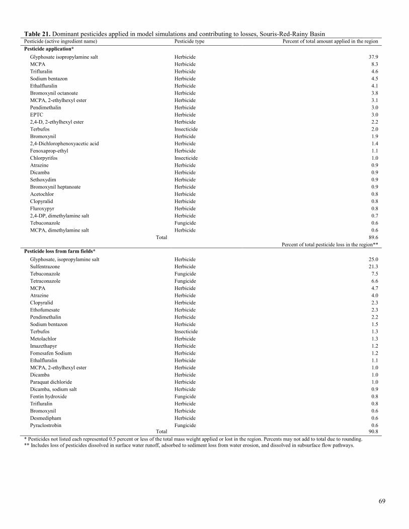
Table 21. Dominant pesticides applied in model simulations and contributing to losses, Souris-Red-Rainy Basin Pesticide (active ingredient name) Pesticide type Percent of total amount applied in the region Pesticide application*

Glyphosate isopropylamine salt Herbicide 37.9 MCPA Herbicide 8.3 Trifluralin Herbicide 4.6 Sodium bentazon Herbicide 4.5 Ethalfluralin Herbicide 4.1 Bromoxynil octanoate Herbicide 3.8 MCPA, 2-ethylhexyl ester Herbicide 3.1 Pendimethalin Herbicide 3.0 EPTC Herbicide 3.0 2,4-D, 2-ethylhexyl ester Herbicide 2.2 Terbufos Insecticide 2.0 Bromoxynil Herbicide 1.9 2,4-Dichlorophenoxyacetic acid Herbicide 1.4 Fenoxaprop-ethyl Herbicide 1.1 Chlorpyrifos Insecticide 1.0 Atrazine Herbicide 0.9 Dicamba Herbicide 0.9 Sethoxydim Herbicide 0.9 Bromoxynil heptanoate Herbicide 0.9 Acetochlor Herbicide 0.8 Clopyralid Herbicide 0.8 Fluroxypyr Herbicide 0.8 2,4-DP, dimethylamine salt Herbicide 0.7 Tebuconazole Fungicide 0.6 MCPA, dimethylamine salt Herbicide 0.6

Total 89.6 Percent of total pesticide loss in the region** Pesticide loss from farm fields*

Glyphosate, isopropylamine salt Herbicide 25.0 Sulfentrazone Herbicide 21.3 Tebuconazole Fungicide 7.5 Tetraconazole Fungicide 6.6 MCPA Herbicide 4.7 Atrazine Herbicide 4.0 Clopyralid Herbicide 2.3 Ethofumesate Herbicide 2.3 Pendimethalin Herbicide 2.2 Sodium bentazon Herbicide 1.5 Terbufos Insecticide 1.3 Metolachlor Herbicide 1.3 Imazethapyr Herbicide 1.2 Fomesafen Sodium Herbicide 1.2 Ethalfluralin Herbicide 1.1 MCPA, 2-ethylhexyl ester Herbicide 1.0 Dicamba Herbicide 1.0 Paraquat dichloride Herbicide 1.0 Dicamba, sodium salt Herbicide 0.9 Fentin hydroxide Fungicide 0.8 Trifluralin Herbicide 0.8 Bromoxynil Herbicide 0.6 Desmedipham Herbicide 0.6 Pyraclostrobin Fungicide 0.6

Total 90.8 * Pesticides not listed each represented 0.5 percent or less of the total mass weight applied or lost in the region. Percents may not add to total due to rounding. ** Includes loss of pesticides dissolved in surface water runoff, adsorbed to sediment loss from water erosion, and dissolved in subsurface flow pathways.

69

Table 22. Field-level effects of conservation practices on pesticide loss and associated edge-of-field environmental risk for cropped acres in the Souris-Red-Rainy Basin

Model simulated outcome

Baseline conservation

condition No-practice

scenario Reduction due

to practices Percent

reduction Pesticide sources

Average annual amount of pesticides applied (grams of active ingredient/hectare) 820 1,160 340 29

Pesticide loss Average annual mass loss of pesticides for all pathways (grams of active

ingredient/hectare) 0.3 0.7 0.4 52 Edge-of-field pesticide risk indicator

Average annual surface water pesticide risk indicator for aquatic ecosystems 0.27 1.19 0.92 78 Average annual surface water pesticide risk indicator for humans 0.02 0.09 0.07 74 Average annual groundwater pesticide risk indicator for humans <0.01 0.01 <0.01 47

Note: Percent reductions were calculated prior to rounding the values for reporting in the table and the associated text. Model simulation results for the baseline conservation condition are presented in appendix B for subregions 0901 and 0902. Effects of conservation practices on pesticide residues and risk Management practices that reduce the potential for loss of pesticides from farm fields consist of a combination of Integrated Pest Management (IPM) techniques and water erosion control practices. Water erosion control practices mitigate the loss of pesticides from farm fields by reducing surface water runoff and sediment loss, both of which carry pesticide residues from the farm field to the surrounding environment. IPM is site-specific in nature, with individual tactics determined by the particular crop/pest/environmental condition. IPM consists of a management strategy for prevention, avoidance, monitoring, and suppression of pest populations. When the use of pesticides is necessary to protect crop yields, selection of pesticides that have the least environmental risk is an important aspect of the suppression component of IPM. Model simulations show that conservation practices—primarily water erosion control practices—are effective in reducing the loss of pesticide residues from farm fields in the Souris-Red-Rainy Basin. Use of conservation practices has reduced the loss of pesticides (summed over all pesticides) by an average of 0.4 gram of active ingredient per hectare per year, a 52-percent reduction from the 0.7 gram per hectare for the no-practice scenario (table 22). However, the total quantity of pesticide residues lost from the field is not the most useful outcome measure for assessing the environmental benefits of conservation practices. The environmental impact is specific to the toxicity of each pesticide to non-target species that may be exposed to the pesticide. Pesticide risk indicators were therefore developed to represent risk at the edge of the field (bottom of soil profile for groundwater). These edge-of-field risk indicators are based on the ratio of average annual pesticide concentrations in water leaving the field to safe concentrations (toxicity thresholds) for each pesticide. As such, these risk indicators do not have units. The pesticide risk indicators were developed so that the relative risk for individual pesticides could be aggregated over

the 110 pesticides included in the model for the Souris-Red-Rainy Basin.21F

22 Risk indicator values of less than 1 are considered “safe” because the annual average concentration is below the toxicity threshold for exposure at the edge of the field.22F

23 Three edge-of-field risk indicators are used here to assess the effects of conservation practices: (1) surface water pesticide risk indicator for aquatic ecosystems, (2) surface water pesticide risk indicator for humans, and (3) groundwater pesticide risk indicator for humans. The surface water risk indicator includes pesticide residues in solution in surface water runoff and in all subsurface water flow pathways that eventually return to surface water (water flow in a surface or tile drainage system, lateral subsurface water flow, and groundwater return flow). The pesticide risk indicator for aquatic ecosystems was based on chronic toxicities for fish and invertebrates, and acute toxicities for algae and vascular aquatic plants. The pesticide risk indicators for humans were based on drinking water standards or the equivalent for pesticides where standards have not been set. These indicators provide a consistent measure that is comparable from field to field and that represents the effects of farming activities on risk reduction without being influenced by other landscape factors. In most environmental settings, however, non-target species are exposed to concentrations that have been diluted by water from other sources, even when those environments are located adjacent to a field. Consequently, these edge-of-field risk indicators cannot be used to predict actual environmental impacts.

22 For a complete documentation of the development of the pesticide risk indicators, see the documentation report “Pesticide risk indicators used in the CEAP cropland modeling,” referenced on page 5.. 23 A threshold value of 1 for the pesticide risk indicator applies when assessing the risk for a single pesticide. Since the indicator is summed over all pesticides in this study, a threshold value of 1 would still apply if pesticide toxicities are additive and no synergistic or antagonistic effects are produced when non-target species are exposed to a mix of pesticides.

70

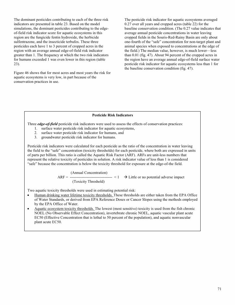
The dominant pesticides contributing to each of the three risk indicators are presented in table 23. Based on the model simulations, the dominant pesticides contributing to the edge-of-field risk indicator score for aquatic ecosystems in this region are the fungicide fentin hydroxide, the herbicide sulfentrazone, and the insecticide terbufos. These three pesticides each have 1 to 3 percent of cropped acres in the region with an average annual edge-of-field risk indicator greater than 1. The frequency at which the two risk indicators for humans exceeded 1 was even lower in this region (table 23). Figure 46 shows that for most acres and most years the risk for aquatic ecosystems is very low, in part because of the conservation practices in use.

The pesticide risk indicator for aquatic ecosystems averaged 0.27 over all years and cropped acres (table 22) for the baseline conservation condition. (The 0.27 value indicates that average annual pesticide concentrations in water leaving cropped fields in the Souris-Red-Rainy Basin are only about one-fourth of the “safe” concentration for non-target plant and animal species when exposed to concentrations at the edge of the field.) The median value, however, is much lower—less than 0.01 (fig. 47). About 94 percent of the cropped acres in the region have an average annual edge-of-field surface water pesticide risk indicator for aquatic ecosystems less than 1 for the baseline conservation condition (fig. 47).

Pesticide Risk Indicators Three edge-of-field pesticide risk indicators were used to assess the effects of conservation practices:

1. surface water pesticide risk indicator for aquatic ecosystems, 2. surface water pesticide risk indicator for humans, and 3. groundwater pesticide risk indicator for humans.

Pesticide risk indicators were calculated for each pesticide as the ratio of the concentration in water leaving the field to the “safe” concentration (toxicity thresholds) for each pesticide, where both are expressed in units of parts per billion. This ratio is called the Aquatic Risk Factor (ARF). ARFs are unit-less numbers that represent the relative toxicity of pesticides in solution. A risk indicator value of less than 1 is considered “safe” because the concentration is below the toxicity threshold for exposure at the edge-of-the field. (Annual Concentration)

ARF = --------------------------------- < 1 Little or no potential adverse impact (Toxicity Threshold)

Two aquatic toxicity thresholds were used in estimating potential risk: • Human drinking water lifetime toxicity thresholds. These thresholds are either taken from the EPA Office

of Water Standards, or derived from EPA Reference Doses or Cancer Slopes using the methods employed by the EPA Office of Water.

• Aquatic ecosystem toxicity thresholds. The lowest (most sensitive) toxicity is used from the fish chronic NOEL (No Observable Effect Concentration), invertebrate chronic NOEL, aquatic vascular plant acute EC50 (Effective Concentration that is lethal to 50 percent of the population), and aquatic nonvascular plant acute EC50.

71

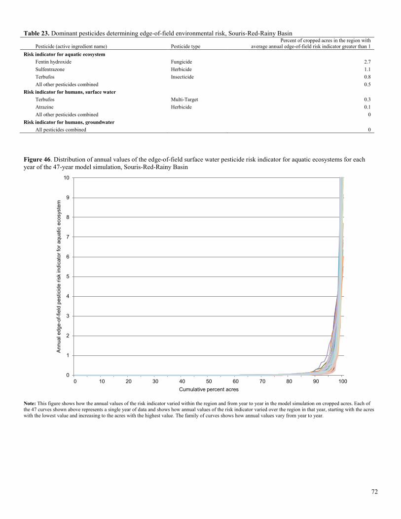
Table 23. Dominant pesticides determining edge-of-field environmental risk, Souris-Red-Rainy Basin

Pesticide (active ingredient name) Pesticide type Percent of cropped acres in the region with

average annual edge-of-field risk indicator greater than 1 Risk indicator for aquatic ecosystem

Fentin hydroxide Fungicide 2.7 Sulfentrazone Herbicide 1.1 Terbufos Insecticide 0.8 All other pesticides combined 0.5

Risk indicator for humans, surface water Terbufos Multi-Target 0.3 Atrazine Herbicide 0.1 All other pesticides combined 0

Risk indicator for humans, groundwater All pesticides combined 0

Figure 46. Distribution of annual values of the edge-of-field surface water pesticide risk indicator for aquatic ecosystems for each year of the 47-year model simulation, Souris-Red-Rainy Basin

Note: This figure shows how the annual values of the risk indicator varied within the region and from year to year in the model simulation on cropped acres. Each of the 47 curves shown above represents a single year of data and shows how annual values of the risk indicator varied over the region in that year, starting with the acres with the lowest value and increasing to the acres with the highest value. The family of curves shows how annual values vary from year to year.

0

1

2

3

4

5

6

7

8

9

10

0 10 20 30 40 50 60 70 80 90 100

Ann

ual e

dge-

of-fi

eld

pest

icid

e ris

k in

dica

tor f

or a

quat

ic e

cosy

stem

Cumulative percent acres

72

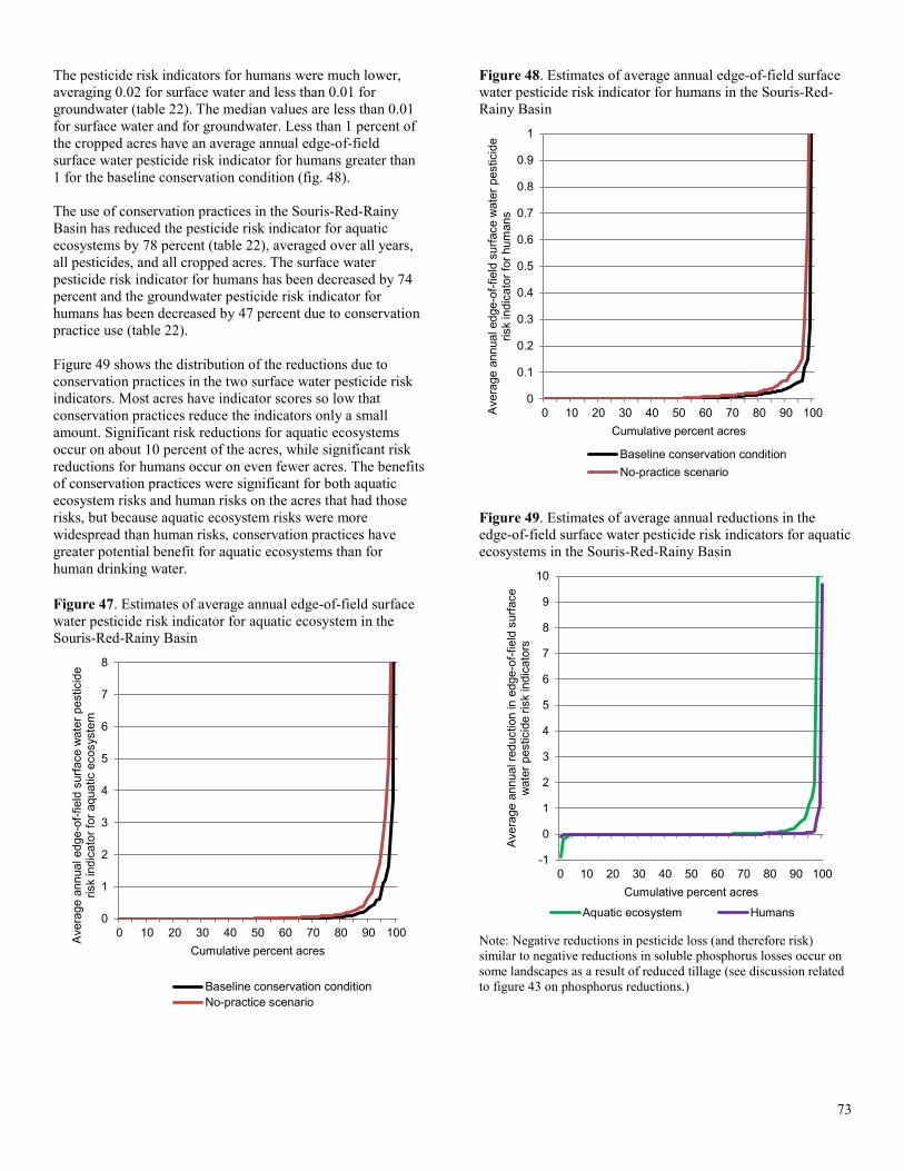
The pesticide risk indicators for humans were much lower, averaging 0.02 for surface water and less than 0.01 for groundwater (table 22). The median values are less than 0.01 for surface water and for groundwater. Less than 1 percent of the cropped acres have an average annual edge-of-field surface water pesticide risk indicator for humans greater than 1 for the baseline conservation condition (fig. 48). The use of conservation practices in the Souris-Red-Rainy Basin has reduced the pesticide risk indicator for aquatic ecosystems by 78 percent (table 22), averaged over all years, all pesticides, and all cropped acres. The surface water pesticide risk indicator for humans has been decreased by 74 percent and the groundwater pesticide risk indicator for humans has been decreased by 47 percent due to conservation practice use (table 22). Figure 49 shows the distribution of the reductions due to conservation practices in the two surface water pesticide risk indicators. Most acres have indicator scores so low that conservation practices reduce the indicators only a small amount. Significant risk reductions for aquatic ecosystems occur on about 10 percent of the acres, while significant risk reductions for humans occur on even fewer acres. The benefits of conservation practices were significant for both aquatic ecosystem risks and human risks on the acres that had those risks, but because aquatic ecosystem risks were more widespread than human risks, conservation practices have greater potential benefit for aquatic ecosystems than for human drinking water. Figure 47. Estimates of average annual edge-of-field surface water pesticide risk indicator for aquatic ecosystem in the Souris-Red-Rainy Basin

Figure 48. Estimates of average annual edge-of-field surface water pesticide risk indicator for humans in the Souris-Red-Rainy Basin

Figure 49. Estimates of average annual reductions in the edge-of-field surface water pesticide risk indicators for aquatic ecosystems in the Souris-Red-Rainy Basin

Note: Negative reductions in pesticide loss (and therefore risk) similar to negative reductions in soluble phosphorus losses occur on some landscapes as a result of reduced tillage (see discussion related to figure 43 on phosphorus reductions.)

0

1

2

3

4

5

6

7

8

0 10 20 30 40 50 60 70 80 90 100Ave

rage

ann

ual e

dge-

of-fi

eld

surfa

ce w

ater

pes

ticid

e ris

k in

dica

tor f

or a

quat

ic e

cosy

stem

Cumulative percent acres

Baseline conservation conditionNo-practice scenario

0

0.1

0.2

0.3

0.4

0.5

0.6

0.7

0.8

0.9

1

0 10 20 30 40 50 60 70 80 90 100Ave

rage

ann

ual e

dge-

of-fi

eld

surfa

ce w

ater

pes

ticid

e ris

k in

dica

tor f

or h

uman

s

Cumulative percent acres

Baseline conservation conditionNo-practice scenario

-1

0

1

2

3

4

5

6

7

8

9

10

0 10 20 30 40 50 60 70 80 90 100

Ave

rage

ann

ual r

educ

tion

in e

dge-

of-fi

eld

surfa

ce

wat

er p

estic

ide

risk

indi

cato

rs

Cumulative percent acres

Aquatic ecosystem Humans

73

Chapter 5 Assessment of Conservation Treatment Needs The adequacy of conservation practices in use in the Souris-Red-Rainy Basin was evaluated to identify remaining conservation treatment needs for controlling wind and water erosion and nutrient loss from fields. The evaluation was based on conservation practice use for the time period 2003 through 2006. Field-level model simulation results for the baseline conservation condition were used to make the assessment. Five resource concerns were evaluated for the Souris-Red-Rainy Basin: 1. sediment loss due to water erosion; 2. nitrogen loss with surface runoff (nitrogen attached to

sediment and in solution); 3. nitrogen loss in subsurface flows; 4. phosphorus lost to surface water (phosphorus attached to

sediment and in solution, including soluble phosphorus in subsurface lateral flow pathways); and

5. wind erosion. The conservation treatment needs for controlling pesticide loss were not evaluated because the assessment requires information on pest infestations, which was not available for the CEAP sample points. A portion of the pesticide residues are controlled by soil erosion control practices; meeting soil erosion control treatment needs would provide partial protection against loss of pesticide residues from farm fields. Integrated Pest Management (IPM) practices are also effective in reducing the risk associated with pesticide residues leaving the farm field. Determination of adequate IPM, however, is highly dependent on the specific site conditions and the nature and extent of the pest problems. Adequate conservation treatment consists of combinations of conservation practices that treat the specific inherent vulnerability factors associated with each field. Not all acres require the same level of conservation treatment. Acres with a high level of inherent vulnerability require more treatment than less vulnerable acres to reduce field-level losses to acceptable levels. Acres with characteristics such as steeper slopes and soil types that promote surface water runoff are more vulnerable to wind erosion and sediment and nutrient losses beyond the edge of the field. Acres that are essentially flat with permeable soil types are more prone to nutrient losses through subsurface flow pathways, most of which return to surface water through drainage ditches, tile drains, natural seeps, and groundwater return flow. The 4.34 million acres with additional conservation treatment needs—undertreated acres—were identified by an imbalance between the level of conservation treatment and the level of inherent vulnerability. Derivation of conservation treatment levels and inherent soil vulnerability classes are described in the next two sections, followed by estimates of undertreated acres.

In summary, findings for the Souris-Red-Rainy Basin indicate that— • 24.7 percent of cropped acres (4.34 million acres) have a

moderate level of need for additional conservation treatment, all for wind erosion, and

• 75.3 percent of cropped acres (13.23 million acres) have a low level of need for additional treatment and are considered to be adequately treated.

Conservation Treatment Levels Drawing from the evaluation of practice use presented in chapter 3, four levels of conservation treatment (high, moderately high, moderate, and low) were defined. For sediment loss due to water erosion, conservation treatment levels were defined by a combination of structural practices and residue and tillage management practices, as defined in figure 50. A high level of water erosion control treatment is in use on about 19 percent of cropped acres, primarily on non-highly erodible land. About 5 percent have a moderately high level of conservation treatment. About 58 percent of cropped acres have a moderate level of conservation treatment for water erosion control. The remaining 17 percent of cropped acres have a low level of conservation treatment for water erosion control in this region. For nitrogen loss with surface runoff, conservation treatment levels were defined by a combination of structural practices, residue and tillage management practices, and nitrogen management practices, as defined in figure 51. A high level of treatment for nitrogen runoff is in use on only 7 percent of cropped acres. About 35 percent have a moderately high level of conservation treatment. The majority of cropped acres—51 percent—have combinations of practices that indicate a moderate level of treatment. About 7 percent of cropped acres have a low level of treatment for nitrogen runoff. For phosphorus lost to surface water, conservation treatment levels were defined by a combination of structural practices, residue and tillage management practices, and phosphorus management practices, as defined in figure 52. A high level of treatment for phosphorus runoff is in use on only 7 percent of the acres. About 35 percent of cropped acres have combinations of practices that indicate a moderately high level of treatment. About 42 percent of cropped acres have a moderate level of treatment, and 16 percent of cropped acres have a low level of phosphorus management. The nitrogen management level presented in figure 9 (see chapter 3) was used to evaluate the adequacy of conservation treatment for nitrogen loss in subsurface flows. A high level of treatment for nitrogen loss in subsurface flows is in use on 37 percent of the acres, and about 36 percent of cropped acres have a moderately high level of treatment. About 23 percent of cropped acres have a moderate level, and only 4 percent have a low level of nitrogen treatment. For wind erosion, a combination of structural practices and tillage intensity was used to evaluate the adequacy of conservation treatment, as defined in figure 53. A high level of

74

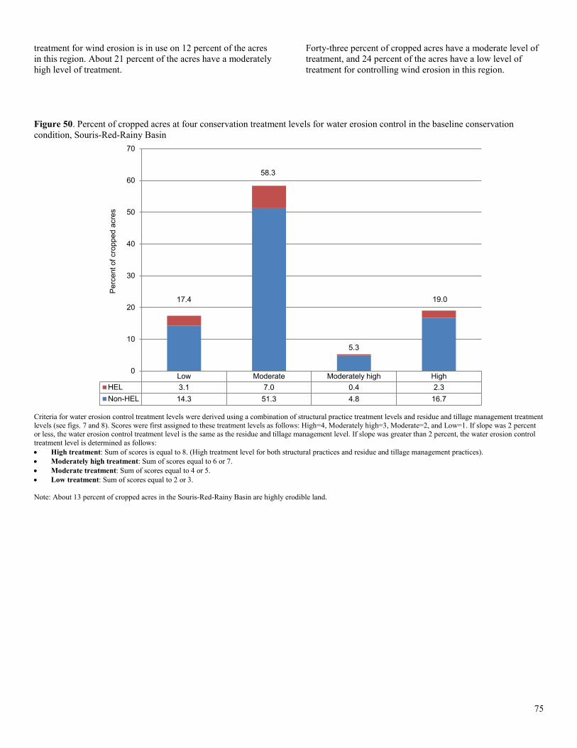
treatment for wind erosion is in use on 12 percent of the acres in this region. About 21 percent of the acres have a moderately high level of treatment.

Forty-three percent of cropped acres have a moderate level of treatment, and 24 percent of the acres have a low level of treatment for controlling wind erosion in this region.

Figure 50. Percent of cropped acres at four conservation treatment levels for water erosion control in the baseline conservation condition, Souris-Red-Rainy Basin

Criteria for water erosion control treatment levels were derived using a combination of structural practice treatment levels and residue and tillage management treatment levels (see figs. 7 and 8). Scores were first assigned to these treatment levels as follows: High=4, Moderately high=3, Moderate=2, and Low=1. If slope was 2 percent or less, the water erosion control treatment level is the same as the residue and tillage management level. If slope was greater than 2 percent, the water erosion control treatment level is determined as follows: • High treatment: Sum of scores is equal to 8. (High treatment level for both structural practices and residue and tillage management practices). • Moderately high treatment: Sum of scores equal to 6 or 7. • Moderate treatment: Sum of scores equal to 4 or 5. • Low treatment: Sum of scores equal to 2 or 3. Note: About 13 percent of cropped acres in the Souris-Red-Rainy Basin are highly erodible land.

Low Moderate Moderately high HighHEL 3.1 7.0 0.4 2.3Non-HEL 14.3 51.3 4.8 16.7

17.4

58.3

5.3

19.0

0

10

20

30

40

50

60

70

Per

cent

of c

ropp

ed a

cres

75

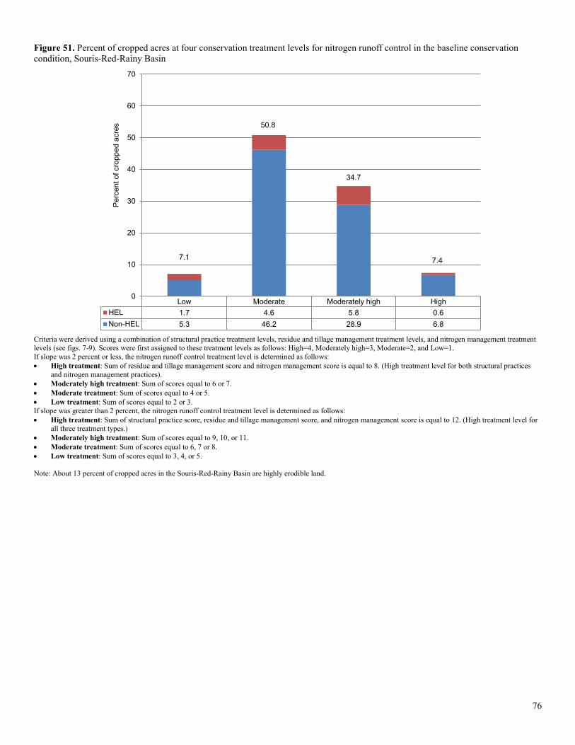
Figure 51. Percent of cropped acres at four conservation treatment levels for nitrogen runoff control in the baseline conservation condition, Souris-Red-Rainy Basin

Criteria were derived using a combination of structural practice treatment levels, residue and tillage management treatment levels, and nitrogen management treatment levels (see figs. 7-9). Scores were first assigned to these treatment levels as follows: High=4, Moderately high=3, Moderate=2, and Low=1. If slope was 2 percent or less, the nitrogen runoff control treatment level is determined as follows: • High treatment: Sum of residue and tillage management score and nitrogen management score is equal to 8. (High treatment level for both structural practices

and nitrogen management practices). • Moderately high treatment: Sum of scores equal to 6 or 7. • Moderate treatment: Sum of scores equal to 4 or 5. • Low treatment: Sum of scores equal to 2 or 3. If slope was greater than 2 percent, the nitrogen runoff control treatment level is determined as follows: • High treatment: Sum of structural practice score, residue and tillage management score, and nitrogen management score is equal to 12. (High treatment level for

all three treatment types.) • Moderately high treatment: Sum of scores equal to 9, 10, or 11. • Moderate treatment: Sum of scores equal to 6, 7 or 8. • Low treatment: Sum of scores equal to 3, 4, or 5. Note: About 13 percent of cropped acres in the Souris-Red-Rainy Basin are highly erodible land.

Low Moderate Moderately high HighHEL 1.7 4.6 5.8 0.6Non-HEL 5.3 46.2 28.9 6.8

7.1

50.8

34.7

7.4

0

10

20

30

40

50

60

70

Per

cent

of c

ropp

ed a

cres

76

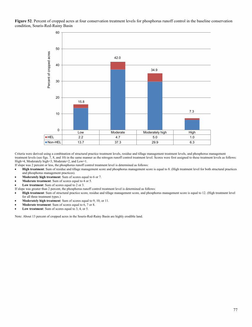
Figure 52. Percent of cropped acres at four conservation treatment levels for phosphorus runoff control in the baseline conservation condition, Souris-Red-Rainy Basin

Criteria were derived using a combination of structural practice treatment levels, residue and tillage management treatment levels, and phosphorus management treatment levels (see figs. 7, 8, and 10) in the same manner as the nitrogen runoff control treatment level. Scores were first assigned to these treatment levels as follows: High=4, Moderately high=3, Moderate=2, and Low=1. If slope was 2 percent or less, the phosphorus runoff control treatment level is determined as follows: • High treatment: Sum of residue and tillage management score and phosphorus management score is equal to 8. (High treatment level for both structural practices

and phosphorus management practices). • Moderately high treatment: Sum of scores equal to 6 or 7. • Moderate treatment: Sum of scores equal to 4 or 5. • Low treatment: Sum of scores equal to 2 or 3. If slope was greater than 2 percent, the phosphorus runoff control treatment level is determined as follows: • High treatment: Sum of structural practice score, residue and tillage management score, and phosphorus management score is equal to 12. (High treatment level

for all three treatment types.) • Moderately high treatment: Sum of scores equal to 9, 10, or 11. • Moderate treatment: Sum of scores equal to 6, 7 or 8. • Low treatment: Sum of scores equal to 3, 4, or 5. Note: About 13 percent of cropped acres in the Souris-Red-Rainy Basin are highly erodible land.

Low Moderate Moderately high HighHEL 2.2 4.7 5.0 1.0Non-HEL 13.7 37.3 29.9 6.3

15.8

42.0

34.9

7.3

0

10

20

30

40

50

60

Per

cent

of c

ropp

ed a

cres

77

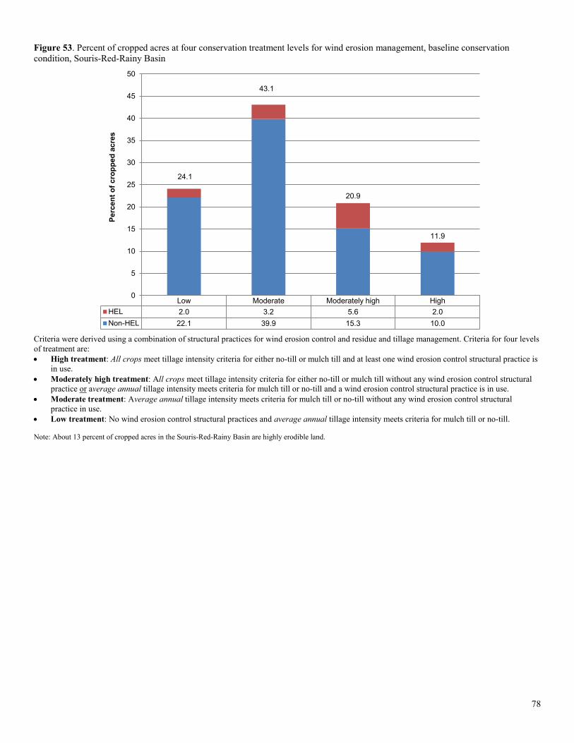
Figure 53. Percent of cropped acres at four conservation treatment levels for wind erosion management, baseline conservation condition, Souris-Red-Rainy Basin

Criteria were derived using a combination of structural practices for wind erosion control and residue and tillage management. Criteria for four levels of treatment are: • High treatment: All crops meet tillage intensity criteria for either no-till or mulch till and at least one wind erosion control structural practice is

in use. • Moderately high treatment: All crops meet tillage intensity criteria for either no-till or mulch till without any wind erosion control structural

practice or average annual tillage intensity meets criteria for mulch till or no-till and a wind erosion control structural practice is in use. • Moderate treatment: Average annual tillage intensity meets criteria for mulch till or no-till without any wind erosion control structural

practice in use. • Low treatment: No wind erosion control structural practices and average annual tillage intensity meets criteria for mulch till or no-till. Note: About 13 percent of cropped acres in the Souris-Red-Rainy Basin are highly erodible land.

Low Moderate Moderately high HighHEL 2.0 3.2 5.6 2.0Non-HEL 22.1 39.9 15.3 10.0

24.1

43.1

20.9

11.9

0

5

10

15

20

25

30

35

40

45

50

Perc

ent o

f cro

pped

acr

es

78

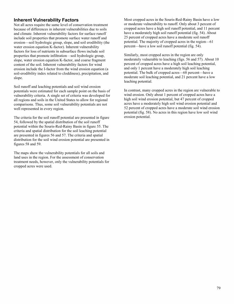
Inherent Vulnerability Factors Not all acres require the same level of conservation treatment because of differences in inherent vulnerabilities due to soils and climate. Inherent vulnerability factors for surface runoff include soil properties that promote surface water runoff and erosion—soil hydrologic group, slope, and soil erodibility (the water erosion equation K-factor). Inherent vulnerability factors for loss of nutrients in subsurface flows include soil properties that promote infiltration—soil hydrologic group, slope, water erosion equation K-factor, and coarse fragment content of the soil. Inherent vulnerability factors for wind erosion include the I-factor from the wind erosion equation (a soil-erodibility index related to cloddiness), precipitation, and slope. Soil runoff and leaching potentials and soil wind erosion potentials were estimated for each sample point on the basis of vulnerability criteria. A single set of criteria was developed for all regions and soils in the United States to allow for regional comparisons. Thus, some soil vulnerability potentials are not well represented in every region. The criteria for the soil runoff potential are presented in figure 54, followed by the spatial distribution of the soil runoff potential within the Souris-Red-Rainy Basin in figure 55. The criteria and spatial distribution for the soil leaching potential are presented in figures 56 and 57. The criteria and spatial distribution for the soil wind erosion potential are presented in figures 58 and 59. The maps show the vulnerability potentials for all soils and land uses in the region. For the assessment of conservation treatment needs, however, only the vulnerability potentials for cropped acres were used.

Most cropped acres in the Souris-Red-Rainy Basin have a low or moderate vulnerability to runoff. Only about 3 percent of cropped acres have a high soil runoff potential, and 11 percent have a moderately high soil runoff potential (fig. 54). About 25 percent of cropped acres have a moderate soil runoff potential. The majority of cropped acres in the region—61 percent—have a low soil runoff potential (fig. 54). Similarly, most cropped acres in the region are only moderately vulnerable to leaching (figs. 56 and 57). About 10 percent of cropped acres have a high soil leaching potential, and only 1 percent have a moderately high soil leaching potential. The bulk of cropped acres—68 percent—have a moderate soil leaching potential, and 21 percent have a low leaching potential. In contrast, many cropped acres in the region are vulnerable to wind erosion. Only about 1 percent of cropped acres have a high soil wind erosion potential, but 47 percent of cropped acres have a moderately high soil wind erosion potential and 52 percent of cropped acres have a moderate soil wind erosion potential (fig. 58). No acres in this region have low soil wind erosion potential.

79

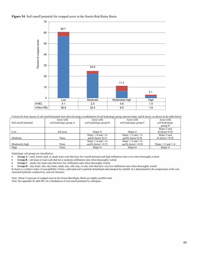
Figure 54. Soil runoff potential for cropped acres in the Souris-Red-Rainy Basin

Criteria for four classes of soil runoff potential were derived using a combination of soil hydrologic group, percent slope, and K-factor, as shown in the table below: Soil runoff potential

Acres with soil hydrologic group A

Acres with soil hydrologic group B

Acres with soil hydrologic group C

Acres with soil hydrologic

group D

Low All acres Slope<4 Slope<2 Slope<2 and

K-factor<0.28

Moderate None Slope >=4 and <=6 and K-factor<0.32

Slope >=2 and <=6 and K-factor<0.28

Slope<2 and K-factor>=0.28

Moderately high None Slope >=4 and <=6 and K-factor>=0.32

Slope >=2 and <=6 and K-factor>=0.28 Slope >=2 and <=4

High None Slope>6 Slope>6 Slope>4 Hydrologic soil groups are classified as: • Group A—sand, loamy sand, or sandy loam soils that have low runoff potential and high infiltration rates even when thoroughly wetted. • Group B—silt loam or loam soils that have moderate infiltration rates when thoroughly wetted. • Group C—sandy clay loam soils that have low infiltration rates when thoroughly wetted. • Group D—clay loam, silty clay loam, sandy clay, silty clay, or clay soils that have very low infiltration rates when thoroughly wetted. K-factor is a relative index of susceptibility of bare, cultivated soil to particle detachment and transport by rainfall. It is determined by the composition of the soil, saturated hydraulic conductivity, and soil structure. Note: About 13 percent of cropped acres in the Souris-Red-Rainy Basin are highly erodible land. Note: See appendix B, table B3, for a breakdown of soil runoff potential by subregion.

Low Moderate Moderately high HighHEL 4.1 2.5 4.8 1.4Non-HEL 56.6 22.4 6.5 1.8

60.7

24.9

11.3

3.1

0

10

20

30

40

50

60

70

Per

cent

of c

ropp

ed a

cres

80

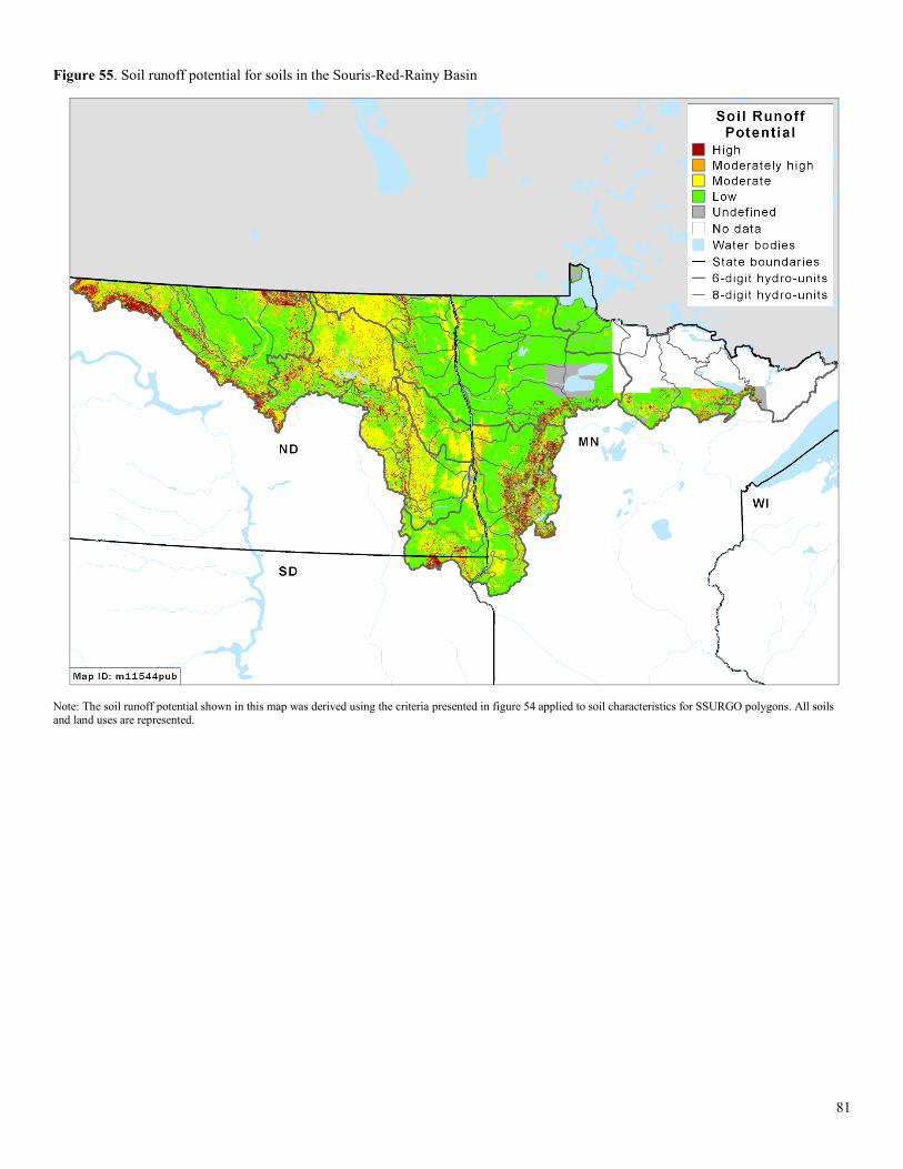
Figure 55. Soil runoff potential for soils in the Souris-Red-Rainy Basin

Note: The soil runoff potential shown in this map was derived using the criteria presented in figure 54 applied to soil characteristics for SSURGO polygons. All soils and land uses are represented.

81

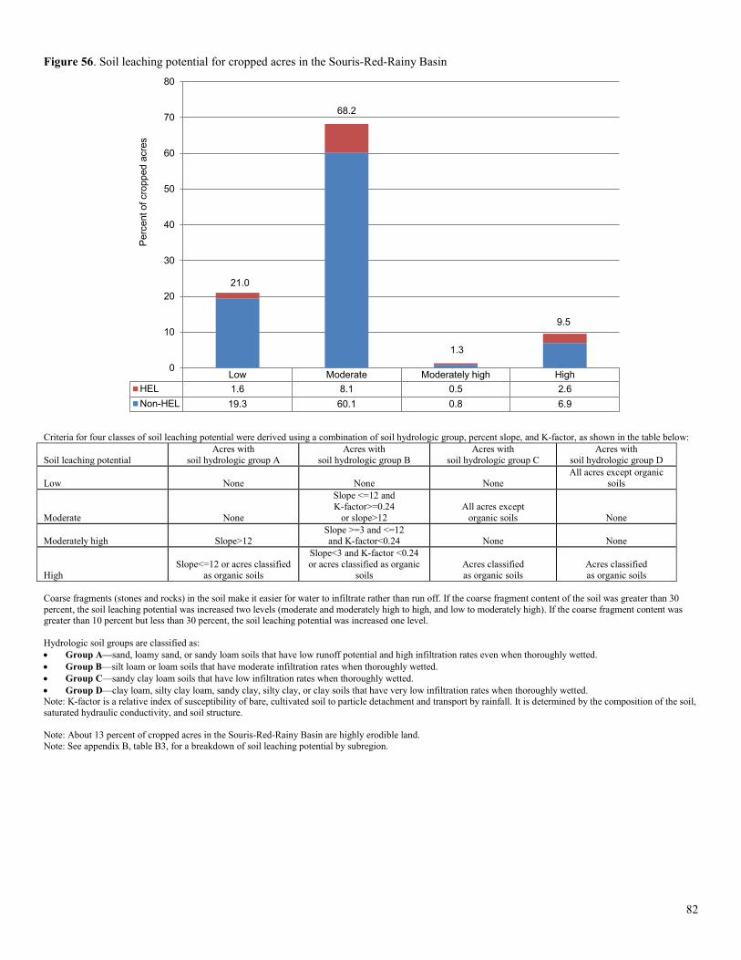
Figure 56. Soil leaching potential for cropped acres in the Souris-Red-Rainy Basin

Criteria for four classes of soil leaching potential were derived using a combination of soil hydrologic group, percent slope, and K-factor, as shown in the table below: Soil leaching potential

Acres with soil hydrologic group A

Acres with soil hydrologic group B

Acres with soil hydrologic group C

Acres with soil hydrologic group D

Low None None None All acres except organic

soils

Moderate None

Slope <=12 and K-factor>=0.24

or slope>12 All acres except

organic soils None

Moderately high Slope>12 Slope >=3 and <=12 and K-factor<0.24 None None

High Slope<=12 or acres classified

as organic soils

Slope<3 and K-factor <0.24 or acres classified as organic

soils Acres classified as organic soils

Acres classified as organic soils

Coarse fragments (stones and rocks) in the soil make it easier for water to infiltrate rather than run off. If the coarse fragment content of the soil was greater than 30 percent, the soil leaching potential was increased two levels (moderate and moderately high to high, and low to moderately high). If the coarse fragment content was greater than 10 percent but less than 30 percent, the soil leaching potential was increased one level. Hydrologic soil groups are classified as: • Group A—sand, loamy sand, or sandy loam soils that have low runoff potential and high infiltration rates even when thoroughly wetted. • Group B—silt loam or loam soils that have moderate infiltration rates when thoroughly wetted. • Group C—sandy clay loam soils that have low infiltration rates when thoroughly wetted. • Group D—clay loam, silty clay loam, sandy clay, silty clay, or clay soils that have very low infiltration rates when thoroughly wetted. Note: K-factor is a relative index of susceptibility of bare, cultivated soil to particle detachment and transport by rainfall. It is determined by the composition of the soil, saturated hydraulic conductivity, and soil structure. Note: About 13 percent of cropped acres in the Souris-Red-Rainy Basin are highly erodible land. Note: See appendix B, table B3, for a breakdown of soil leaching potential by subregion.

Low Moderate Moderately high HighHEL 1.6 8.1 0.5 2.6Non-HEL 19.3 60.1 0.8 6.9

21.0

68.2

1.3

9.5

0

10

20

30

40

50

60

70

80

Per

cent

of c

ropp

ed a

cres

82

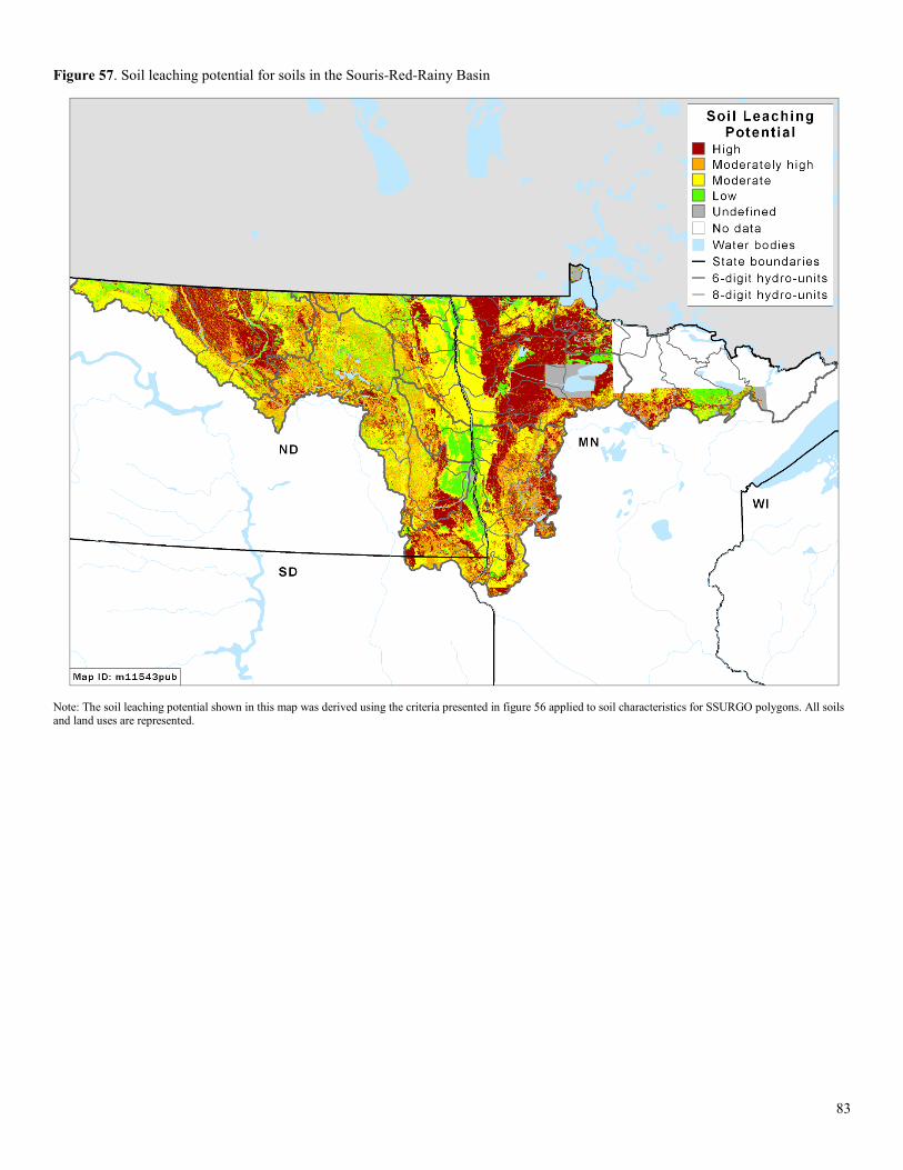
Figure 57. Soil leaching potential for soils in the Souris-Red-Rainy Basin

Note: The soil leaching potential shown in this map was derived using the criteria presented in figure 56 applied to soil characteristics for SSURGO polygons. All soils and land uses are represented.

83

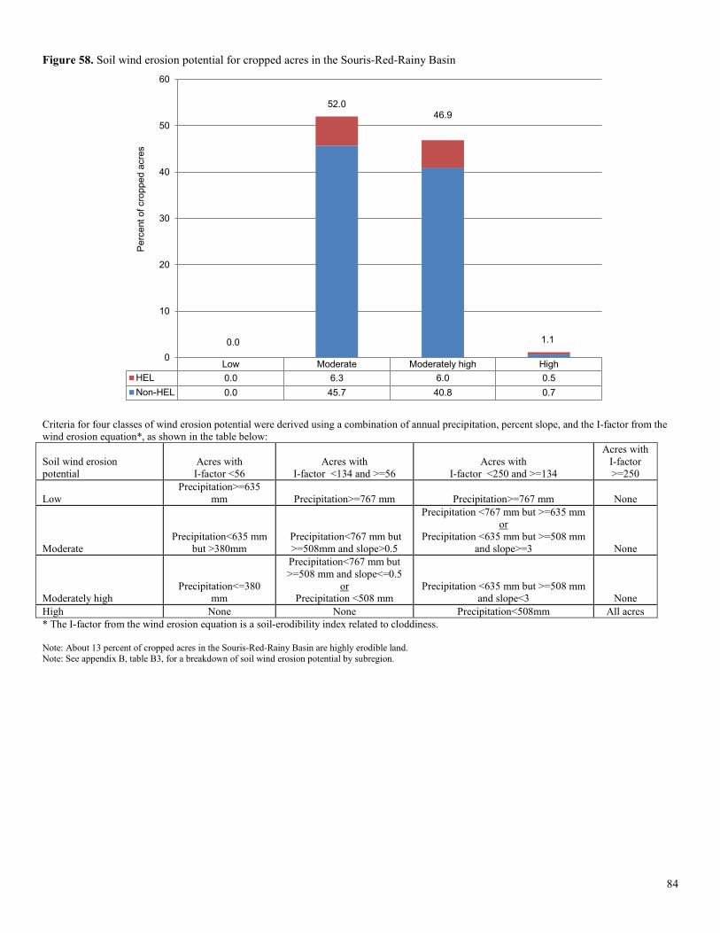
Figure 58. Soil wind erosion potential for cropped acres in the Souris-Red-Rainy Basin

Criteria for four classes of wind erosion potential were derived using a combination of annual precipitation, percent slope, and the I-factor from the wind erosion equation*, as shown in the table below: Soil wind erosion potential

Acres with I-factor <56

Acres with I-factor <134 and >=56

Acres with I-factor <250 and >=134

Acres with I-factor >=250

Low Precipitation>=635

mm Precipitation>=767 mm Precipitation>=767 mm None

Moderate Precipitation<635 mm

but >380mm Precipitation<767 mm but >=508mm and slope>0.5

Precipitation <767 mm but >=635 mm or

Precipitation <635 mm but >=508 mm and slope>=3 None

Moderately high Precipitation<=380

mm

Precipitation<767 mm but >=508 mm and slope<=0.5

or Precipitation <508 mm

Precipitation <635 mm but >=508 mm and slope<3 None

High None None Precipitation<508mm All acres * The I-factor from the wind erosion equation is a soil-erodibility index related to cloddiness. Note: About 13 percent of cropped acres in the Souris-Red-Rainy Basin are highly erodible land. Note: See appendix B, table B3, for a breakdown of soil wind erosion potential by subregion.

Low Moderate Moderately high HighHEL 0.0 6.3 6.0 0.5Non-HEL 0.0 45.7 40.8 0.7

0.0

52.0 46.9

1.1

0

10

20

30

40

50

60

Per

cent

of c

ropp

ed a

cres

84

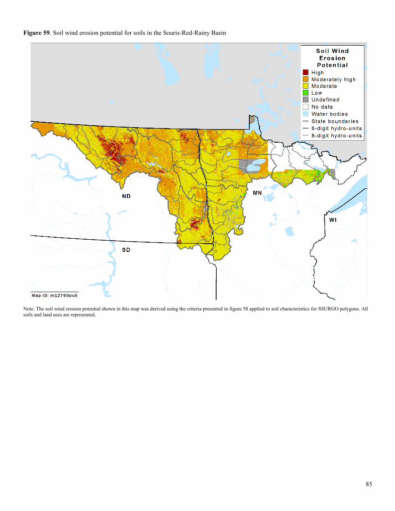
Figure 59. Soil wind erosion potential for soils in the Souris-Red-Rainy Basin

Note: The soil wind erosion potential shown in this map was derived using the criteria presented in figure 58 applied to soil characteristics for SSURGO polygons. All soils and land uses are represented.

85

Evaluation of Conservation Treatment The “matrix approach” A “matrix approach” was used to identify acres where the level of conservation treatment is inadequate relative to the level of inherent vulnerability. These acres are referred to as “under-treated acres.” Cropped acres were divided into 16 groups—defined by the four soil vulnerability potentials and four conservation treatment levels. The evaluation of conservation treatment needs was conducted by identifying which of the 16 groups of acres are inadequately treated with respect to the vulnerability potential. The matrixes are presented for each of the five resource concerns in tables 24 through 28. Each table includes seven sets of matrixes that, taken together, capture the effects of conservation practices in the region and identify the need for additional conservation treatment. Acres and model results for each of the 16 groupings are presented in the first five matrixes in each table. The combination of the four soil vulnerability potentials and the four conservation treatment levels separates the acres with high losses from the acres with low losses. There generally is a trend of decreasing losses with increasing conservation treatment levels within each vulnerability potential. The tables also demonstrate that the high and moderately high treatment levels are effective in reducing losses at all vulnerability potentials. The last two matrixes in each table show how conservation treatment needs were identified. Three levels of conservation treatment need were defined. • Acres with a “high” level of need for conservation

treatment consist of the most critical under-treated acres in the region. These are the most vulnerable of the under-treated acres with the least conservation treatment and have the highest erosion and/or loss of nutrients.

• Acres with a “moderate” level of need for conservation treatment consist of under-treated acres that generally have lower levels of vulnerability or have more conservation practice use than acres with a high level of need. The treatment level required is not necessarily less, although it can be, but rather the soil and nutrient losses are lower and thus there is less potential on a per-acre basis for reducing agricultural pollutant loadings with additional conservation treatment.

• Acres with a “low” level of need for conservation treatment consist of acres that are adequately treated with respect to the level of inherent vulnerability. While gains can be attained by adding conservation practices to some of these acres, additional conservation treatment would reduce field losses by only a small amount.

Specific criteria were used to identify the groups of acres that fall into each of the three levels of conservation treatment need. Criteria were not tailored to a specific region, but were derived for use in all regions of the country to allow for comparisons of under-treated acres across regions using a consistent analytical framework.

The criteria and steps in the process are as follows— 1. The percentage of acres that exceeded a given level of

loss was estimated for each cell in the matrix as a guide to determining the extent of excessive losses. These are referred to as “acceptable levels.” Losses above these levels were treated as unacceptable levels of loss. “Acceptable levels”23F

24 for field-level losses used in this study are— o Average of 2 tons per acre per year for sediment loss, o Average of 15 pounds per acre per year for nitrogen

loss with surface runoff (soluble and sediment attached),

o Average of 25 pounds per acre per year for nitrogen loss in subsurface flows,

o Average of 4 pounds per acre per year for phosphorus lost to surface water (soluble and sediment attached), and

o Average wind erosion rate of 4 tons per acre per year. 2. Groups of acres with less than 30 percent of the acres

exceeding acceptable levels were defined as adequately treated acres and designated as having a low level of conservation treatment need.

3. Groups of acres with more than 60 percent of the acres in excess of acceptable levels were designated as having a high level of conservation treatment need, indicated by darker shaded cells in the matrixes.

4. The remaining acres were designated as having a moderate level of conservation treatment need, indicated by lighter shaded cells in the matrix.

Under-treated acres—those groups of acres with either a high or moderate level of conservation treatment need—are shown in the last matrix in each table. In most cases, under-treated acres consist of acres where the conservation treatment level was one step or more below the soil vulnerability potential. Acceptable levels were initially derived through a series of forums held at professional meetings of researchers working on fate and transport of sediment and nutrients in agriculture. Those meetings produced a range of estimates representing what could be realistically achieved with today’s production and conservation technologies. The range was narrowed by further examination of APEX model output, which also showed that the levels selected were agronomically feasible in all agricultural regions of the country. The criteria used to identify acres that need additional conservation treatment, including acceptable levels, are not intended to provide adequate protection of water quality, although for some environmental settings they may be suitable for that purpose. Evaluation of how much conservation treatment is needed to meet Federal, State, and/or local water quality goals in the region is beyond the scope of this study.

24 The long-term average loss was used as the criteria because losses vary considerably from year to year, and the evaluation is intended to assess the adequacy of conservation treatment over all years, on average. Average annual losses derived from APEX model output simulated over 47 years of actual weather (1960 through 2006) were compared to the acceptable level criteria for each sample point.

86

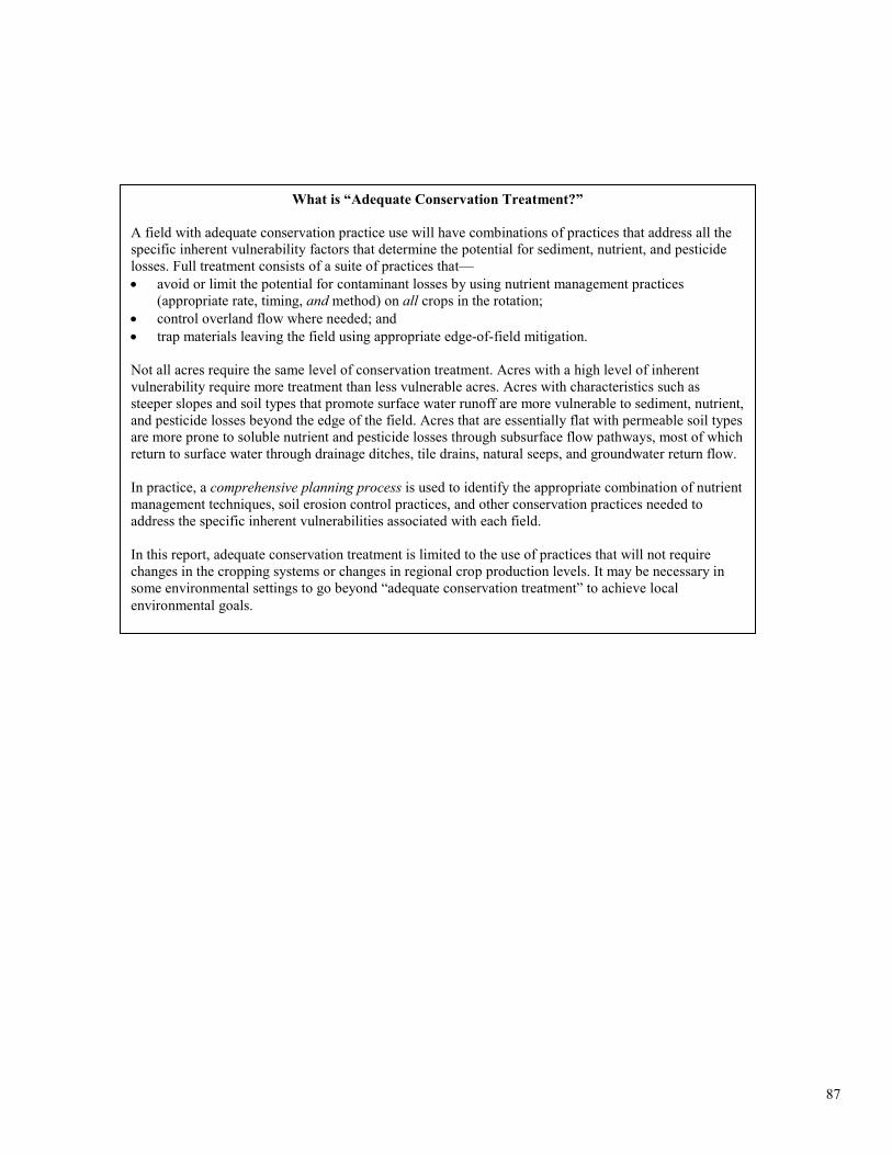
What is “Adequate Conservation Treatment?”

A field with adequate conservation practice use will have combinations of practices that address all the specific inherent vulnerability factors that determine the potential for sediment, nutrient, and pesticide losses. Full treatment consists of a suite of practices that— • avoid or limit the potential for contaminant losses by using nutrient management practices

(appropriate rate, timing, and method) on all crops in the rotation; • control overland flow where needed; and • trap materials leaving the field using appropriate edge-of-field mitigation. Not all acres require the same level of conservation treatment. Acres with a high level of inherent vulnerability require more treatment than less vulnerable acres. Acres with characteristics such as steeper slopes and soil types that promote surface water runoff are more vulnerable to sediment, nutrient, and pesticide losses beyond the edge of the field. Acres that are essentially flat with permeable soil types are more prone to soluble nutrient and pesticide losses through subsurface flow pathways, most of which return to surface water through drainage ditches, tile drains, natural seeps, and groundwater return flow. In practice, a comprehensive planning process is used to identify the appropriate combination of nutrient management techniques, soil erosion control practices, and other conservation practices needed to address the specific inherent vulnerabilities associated with each field. In this report, adequate conservation treatment is limited to the use of practices that will not require changes in the cropping systems or changes in regional crop production levels. It may be necessary in some environmental settings to go beyond “adequate conservation treatment” to achieve local environmental goals.

87

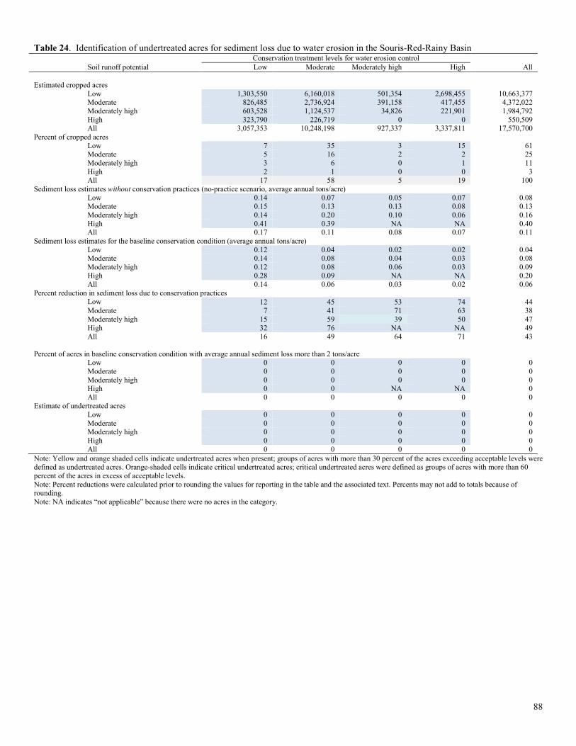
Table 24. Identification of undertreated acres for sediment loss due to water erosion in the Souris-Red-Rainy Basin Conservation treatment levels for water erosion control Soil runoff potential Low Moderate Moderately high High All Estimated cropped acres Low 1,303,550 6,160,018 501,354 2,698,455 10,663,377 Moderate 826,485 2,736,924 391,158 417,455 4,372,022 Moderately high 603,528 1,124,537 34,826 221,901 1,984,792 High 323,790 226,719 0 0 550,509 All 3,057,353 10,248,198 927,337 3,337,811 17,570,700 Percent of cropped acres Low 7 35 3 15 61 Moderate 5 16 2 2 25 Moderately high 3 6 0 1 11 High 2 1 0 0 3 All 17 58 5 19 100 Sediment loss estimates without conservation practices (no-practice scenario, average annual tons/acre) Low 0.14 0.07 0.05 0.07 0.08 Moderate 0.15 0.13 0.13 0.08 0.13 Moderately high 0.14 0.20 0.10 0.06 0.16 High 0.41 0.39 NA NA 0.40 All 0.17 0.11 0.08 0.07 0.11 Sediment loss estimates for the baseline conservation condition (average annual tons/acre) Low 0.12 0.04 0.02 0.02 0.04 Moderate 0.14 0.08 0.04 0.03 0.08 Moderately high 0.12 0.08 0.06 0.03 0.09 High 0.28 0.09 NA NA 0.20 All 0.14 0.06 0.03 0.02 0.06 Percent reduction in sediment loss due to conservation practices Low 12 45 53 74 44 Moderate 7 41 71 63 38 Moderately high 15 59 39 50 47 High 32 76 NA NA 49 All 16 49 64 71 43 Percent of acres in baseline conservation condition with average annual sediment loss more than 2 tons/acre Low 0 0 0 0 0 Moderate 0 0 0 0 0 Moderately high 0 0 0 0 0 High 0 0 NA NA 0 All 0 0 0 0 0 Estimate of undertreated acres Low 0 0 0 0 0 Moderate 0 0 0 0 0 Moderately high 0 0 0 0 0 High 0 0 0 0 0 All 0 0 0 0 0 Note: Yellow and orange shaded cells indicate undertreated acres when present; groups of acres with more than 30 percent of the acres exceeding acceptable levels were defined as undertreated acres. Orange-shaded cells indicate critical undertreated acres; critical undertreated acres were defined as groups of acres with more than 60 percent of the acres in excess of acceptable levels. Note: Percent reductions were calculated prior to rounding the values for reporting in the table and the associated text. Percents may not add to totals because of rounding. Note: NA indicates “not applicable” because there were no acres in the category.

88

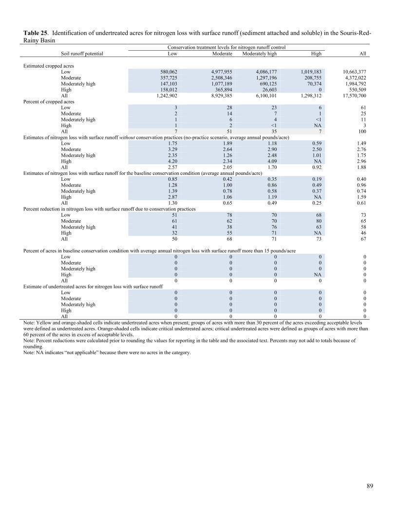
Table 25. Identification of undertreated acres for nitrogen loss with surface runoff (sediment attached and soluble) in the Souris-Red-Rainy Basin Conservation treatment levels for nitrogen runoff control Soil runoff potential Low Moderate Moderately high High All Estimated cropped acres Low 580,062 4,977,955 4,086,177 1,019,183 10,663,377 Moderate 357,725 2,508,346 1,297,196 208,755 4,372,022 Moderately high 147,103 1,077,189 690,125 70,374 1,984,792 High 158,012 365,894 26,603 0 550,509 All 1,242,902 8,929,385 6,100,101 1,298,312 17,570,700 Percent of cropped acres Low 3 28 23 6 61 Moderate 2 14 7 1 25 Moderately high 1 6 4 <1 11 High 1 2 <1 NA 3 All 7 51 35 7 100 Estimates of nitrogen loss with surface runoff without conservation practices (no-practice scenario, average annual pounds/acre) Low 1.75 1.89 1.18 0.59 1.49 Moderate 3.29 2.64 2.90 2.50 2.76 Moderately high 2.35 1.26 2.48 1.01 1.75 High 4.20 2.34 4.09 NA 2.96 All 2.57 2.05 1.70 0.92 1.88 Estimates of nitrogen loss with surface runoff for the baseline conservation condition (average annual pounds/acre) Low 0.85 0.42 0.35 0.19 0.40 Moderate 1.28 1.00 0.86 0.49 0.96 Moderately high 1.39 0.78 0.58 0.37 0.74 High 2.87 1.06 1.19 NA 1.59 All 1.30 0.65 0.49 0.25 0.61 Percent reduction in nitrogen loss with surface runoff due to conservation practices Low 51 78 70 68 73 Moderate 61 62 70 80 65 Moderately high 41 38 76 63 58 High 32 55 71 NA 46 All 50 68 71 73 67 Percent of acres in baseline conservation condition with average annual nitrogen loss with surface runoff more than 15 pounds/acre Low 0 0 0 0 0 Moderate 0 0 0 0 0 Moderately high 0 0 0 0 0 High 0 0 0 NA 0 All 0 0 0 0 0 Estimate of undertreated acres for nitrogen loss with surface runoff Low 0 0 0 0 0 Moderate 0 0 0 0 0 Moderately high 0 0 0 0 0 High 0 0 0 0 0 All 0 0 0 0 0 Note: Yellow and orange-shaded cells indicate undertreated acres when present; groups of acres with more than 30 percent of the acres exceeding acceptable levels were defined as undertreated acres. Orange-shaded cells indicate critical undertreated acres; critical undertreated acres were defined as groups of acres with more than 60 percent of the acres in excess of acceptable levels. Note: Percent reductions were calculated prior to rounding the values for reporting in the table and the associated text. Percents may not add to totals because of rounding. Note: NA indicates “not applicable” because there were no acres in the category.

89

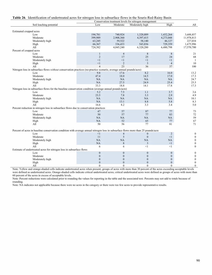
Table 26. Identification of undertreated acres for nitrogen loss in subsurface flows in the Souris-Red-Rainy Basin Conservation treatment levels for nitrogen management Soil leaching potential Low Moderate Moderately high High All Estimated cropped acres Low 194,781 740,924 1,320,889 1,432,264 3,688,857 Moderate 399,989 2,908,360 4,397,415 4,273,048 11,978,813 Moderately high 63,245 59,522 58,140 46,127 227,034 High 66,367 336,433 543,836 729,359 1,675,996 All 724,382 4,045,240 6,320,280 6,480,798 17,570,700 Percent of cropped acres Low 1 4 8 8 21 Moderate 2 17 25 24 68 Moderately high <1 <1 <1 <1 1 High <1 2 3 4 10 All 4 23 36 37 100 Nitrogen loss in subsurface flows without conservation practices (no-practice scenario, average annual pounds/acre) Low 9.8 17.6 8.2 16.0 13.2 Moderate 47.4 18.0 14.5 17.0 17.3 Moderately high NA NA NA NA 24.7 High NA 27.5 24.9 25.4 25.5 All 33.3 18.8 14.1 17.8 17.3 Nitrogen loss in subsurface flows for the baseline conservation condition (average annual pounds/acre) Low 5.2 7.5 1.1 3.7 3.6 Moderate 23.5 7.8 3.3 2.9 4.9 Moderately high NA NA NA NA 10.1 High NA 13.1 8.8 5.8 8.3 All 16.6 8.2 3.3 3.4 5.0 Percent reduction in nitrogen loss in subsurface flows due to conservation practices Low 47 57 87 77 73 Moderate 50 57 77 83 72 Moderately high NA NA NA NA 59 High NA 52 65 77 67 All 50 56 77 81 71 Percent of acres in baseline conservation condition with average annual nitrogen loss in subsurface flows more than 25 pounds/acre Low <1 4 0 2 0 Moderate 11 5 0 <1 0 Moderately high NA NA NA NA 0 High NA 8 3 <1 0 All 6 6 <1 <1 0 Estimate of undertreated acres for nitrogen loss in subsurface flows Low 0 0 0 0 0 Moderate 0 0 0 0 0 Moderately high 0 0 0 0 0 High 0 0 0 0 0 All 0 0 0 0 0 Note: Yellow and orange-shaded cells indicate undertreated acres when present; groups of acres with more than 30 percent of the acres exceeding acceptable levels were defined as undertreated acres. Orange-shaded cells indicate critical undertreated acres; critical undertreated acres were defined as groups of acres with more than 60 percent of the acres in excess of acceptable levels. Note: Percent reductions were calculated prior to rounding the values for reporting in the table and the associated text. Percents may not add to totals because of rounding. Note: NA indicates not applicable because there were no acres in the category or there were too few acres to provide representative results.

90

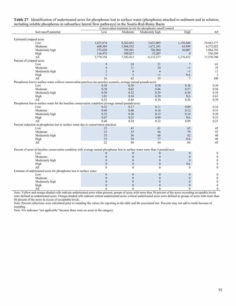
Table 27. Identification of undertreated acres for phosphorus lost to surface water (phosphorus attached to sediment and in solution, including soluble phosphorus in subsurface lateral flow pathways) in the Souris-Red-Rainy Basin Conservation treatment levels for phosphorus runoff control Soil runoff potential Low Moderate Moderately high High All Estimated cropped acres Low 1,621,674 4,263,852 3,621,005 1,156,846 10,663,377 Moderate 668,389 1,968,532 1,671,101 63,999 4,372,022 Moderately high 372,620 769,201 786,964 56,007 1,984,792 High 116,475 380,827 53,207 0 550,509 All 2,779,158 7,382,413 6,132,277 1,276,852 17,570,700 Percent of cropped acres Low 9 24 21 7 61 Moderate 4 11 10 <1 25 Moderately high 2 4 4 <1 11 High 1 2 <1 NA 3 All 16 42 35 7 100 Phosphorus lost to surface water without conservation practices (no-practice scenario, average annual pounds/acre) Low 0.38 0.30 0.28 0.26 0.30 Moderate 0.78 0.62 0.46 0.57 0.58 Moderately high 0.50 0.32 0.39 0.36 0.38 High 1.01 0.54 0.39 NA 0.63 All 0.52 0.40 0.34 0.28 0.39 Phosphorus lost to surface water for the baseline conservation condition (average annual pounds/acre) Low 0.32 0.17 0.11 0.09 0.16 Moderate 0.60 0.40 0.16 0.12 0.33 Moderately high 0.33 0.20 0.13 0.14 0.20 High 0.67 0.25 0.09 NA 0.32 All 0.40 0.24 0.12 0.09 0.21 Percent reduction in phosphorus lost to surface water due to conservation practices Low 15 43 61 65 45 Moderate 23 35 66 79 43 Moderately high 33 36 66 62 48 High 33 54 77 NA 48 All 22 40 64 66 45 Percent of acres in baseline conservation condition with average annual phosphorus lost to surface water more than 4 pounds/acre Low 0 0 0 0 0 Moderate 0 0 0 0 0 Moderately high 0 0 0 0 0 High 0 0 0 NA 0 All 0 0 0 0 0 Estimate of undertreated acres for phosphorus lost to surface water Low 0 0 0 0 0 Moderate 0 0 0 0 0 Moderately high 0 0 0 0 0 High 0 0 0 0 0 All 0 0 0 0 0 Note: Yellow and orange-shaded cells indicate undertreated acres when present; groups of acres with more than 30 percent of the acres exceeding acceptable levels were defined as undertreated acres. Orange-shaded cells indicate critical undertreated acres; critical undertreated acres were defined as groups of acres with more than 60 percent of the acres in excess of acceptable levels. Note: Percent reductions were calculated prior to rounding the values for reporting in the table and the associated text. Percents may not add to totals because of rounding. Note: NA indicates “not applicable” because there were no acres in the category.

91

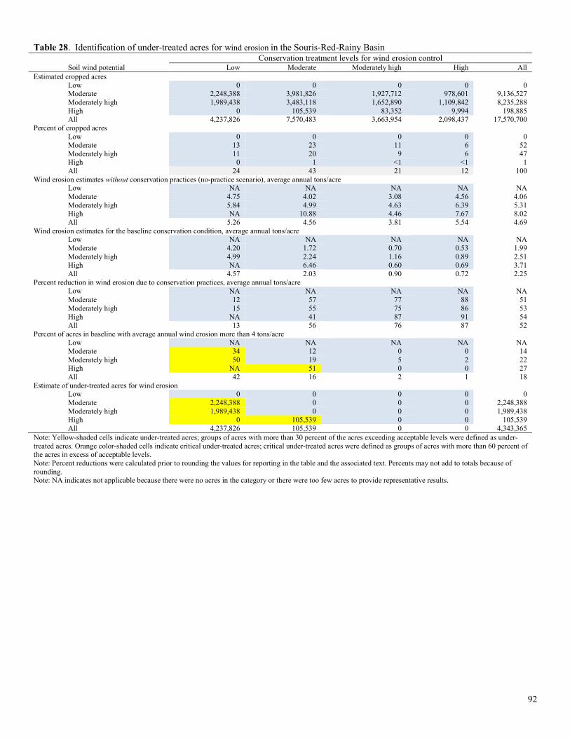
Table 28. Identification of under-treated acres for wind erosion in the Souris-Red-Rainy Basin Conservation treatment levels for wind erosion control Soil wind potential Low Moderate Moderately high High All Estimated cropped acres Low 0 0 0 0 0 Moderate 2,248,388 3,981,826 1,927,712 978,601 9,136,527 Moderately high 1,989,438 3,483,118 1,652,890 1,109,842 8,235,288 High 0 105,539 83,352 9,994 198,885 All 4,237,826 7,570,483 3,663,954 2,098,437 17,570,700 Percent of cropped acres Low 0 0 0 0 0 Moderate 13 23 11 6 52 Moderately high 11 20 9 6 47 High 0 1 <1 <1 1 All 24 43 21 12 100 Wind erosion estimates without conservation practices (no-practice scenario), average annual tons/acre Low NA NA NA NA NA Moderate 4.75 4.02 3.08 4.56 4.06 Moderately high 5.84 4.99 4.63 6.39 5.31 High NA 10.88 4.46 7.67 8.02 All 5.26 4.56 3.81 5.54 4.69 Wind erosion estimates for the baseline conservation condition, average annual tons/acre Low NA NA NA NA NA Moderate 4.20 1.72 0.70 0.53 1.99 Moderately high 4.99 2.24 1.16 0.89 2.51 High NA 6.46 0.60 0.69 3.71 All 4.57 2.03 0.90 0.72 2.25 Percent reduction in wind erosion due to conservation practices, average annual tons/acre Low NA NA NA NA NA Moderate 12 57 77 88 51 Moderately high 15 55 75 86 53 High NA 41 87 91 54 All 13 56 76 87 52 Percent of acres in baseline with average annual wind erosion more than 4 tons/acre Low NA NA NA NA NA Moderate 34 12 0 0 14 Moderately high 50 19 5 2 22 High NA 51 0 0 27 All 42 16 2 1 18 Estimate of under-treated acres for wind erosion Low 0 0 0 0 0 Moderate 2,248,388 0 0 0 2,248,388 Moderately high 1,989,438 0 0 0 1,989,438 High 0 105,539 0 0 105,539 All 4,237,826 105,539 0 0 4,343,365 Note: Yellow-shaded cells indicate under-treated acres; groups of acres with more than 30 percent of the acres exceeding acceptable levels were defined as under-treated acres. Orange color-shaded cells indicate critical under-treated acres; critical under-treated acres were defined as groups of acres with more than 60 percent of the acres in excess of acceptable levels. Note: Percent reductions were calculated prior to rounding the values for reporting in the table and the associated text. Percents may not add to totals because of rounding. Note: NA indicates not applicable because there were no acres in the category or there were too few acres to provide representative results.

92

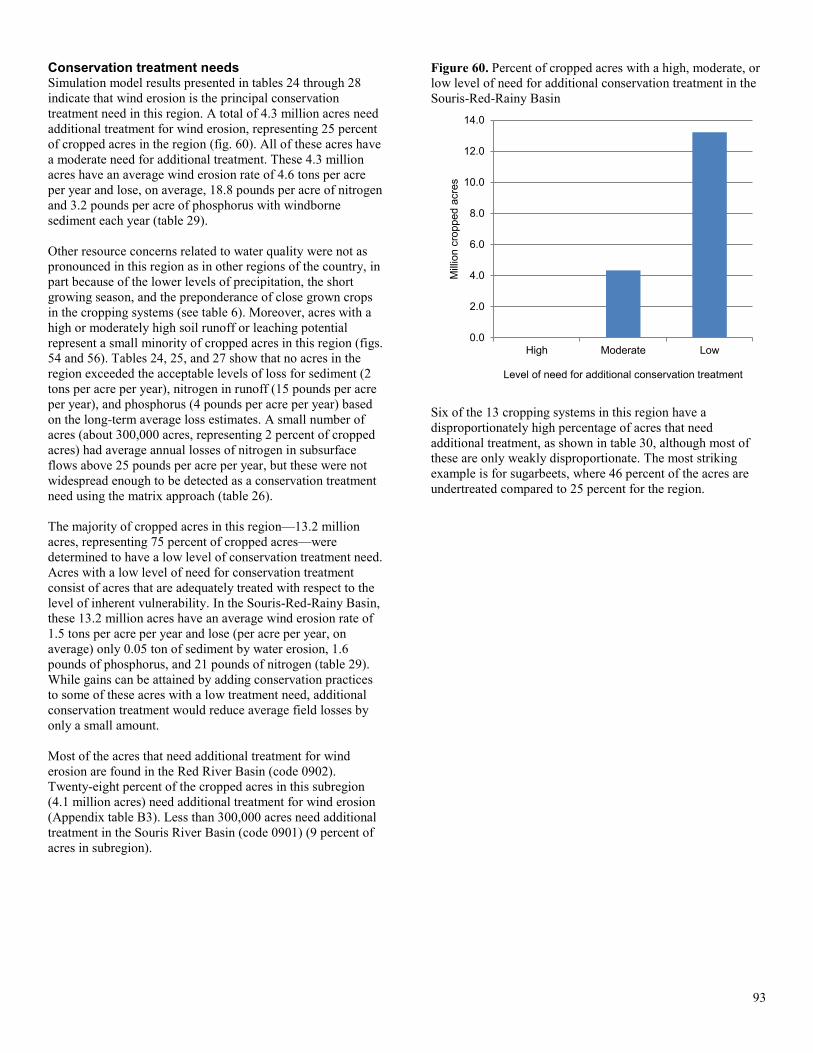
Conservation treatment needs Simulation model results presented in tables 24 through 28 indicate that wind erosion is the principal conservation treatment need in this region. A total of 4.3 million acres need additional treatment for wind erosion, representing 25 percent of cropped acres in the region (fig. 60). All of these acres have a moderate need for additional treatment. These 4.3 million acres have an average wind erosion rate of 4.6 tons per acre per year and lose, on average, 18.8 pounds per acre of nitrogen and 3.2 pounds per acre of phosphorus with windborne sediment each year (table 29). Other resource concerns related to water quality were not as pronounced in this region as in other regions of the country, in part because of the lower levels of precipitation, the short growing season, and the preponderance of close grown crops in the cropping systems (see table 6). Moreover, acres with a high or moderately high soil runoff or leaching potential represent a small minority of cropped acres in this region (figs. 54 and 56). Tables 24, 25, and 27 show that no acres in the region exceeded the acceptable levels of loss for sediment (2 tons per acre per year), nitrogen in runoff (15 pounds per acre per year), and phosphorus (4 pounds per acre per year) based on the long-term average loss estimates. A small number of acres (about 300,000 acres, representing 2 percent of cropped acres) had average annual losses of nitrogen in subsurface flows above 25 pounds per acre per year, but these were not widespread enough to be detected as a conservation treatment need using the matrix approach (table 26). The majority of cropped acres in this region—13.2 million acres, representing 75 percent of cropped acres—were determined to have a low level of conservation treatment need. Acres with a low level of need for conservation treatment consist of acres that are adequately treated with respect to the level of inherent vulnerability. In the Souris-Red-Rainy Basin, these 13.2 million acres have an average wind erosion rate of 1.5 tons per acre per year and lose (per acre per year, on average) only 0.05 ton of sediment by water erosion, 1.6 pounds of phosphorus, and 21 pounds of nitrogen (table 29). While gains can be attained by adding conservation practices to some of these acres with a low treatment need, additional conservation treatment would reduce average field losses by only a small amount. Most of the acres that need additional treatment for wind erosion are found in the Red River Basin (code 0902). Twenty-eight percent of the cropped acres in this subregion (4.1 million acres) need additional treatment for wind erosion (Appendix table B3). Less than 300,000 acres need additional treatment in the Souris River Basin (code 0901) (9 percent of acres in subregion).

Figure 60. Percent of cropped acres with a high, moderate, or low level of need for additional conservation treatment in the Souris-Red-Rainy Basin

Six of the 13 cropping systems in this region have a disproportionately high percentage of acres that need additional treatment, as shown in table 30, although most of these are only weakly disproportionate. The most striking example is for sugarbeets, where 46 percent of the acres are undertreated compared to 25 percent for the region.

0.0

2.0

4.0

6.0

8.0

10.0

12.0

14.0

High Moderate Low

Mill

ion

crop

ped

acre

s

Level of need for additional conservation treatment

93

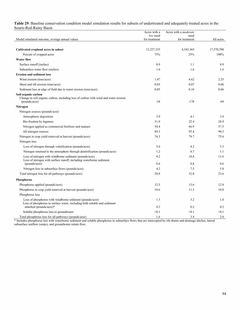
Table 29. Baseline conservation condition model simulation results for subsets of undertreated and adequately treated acres in the Souris-Red-Rainy Basin

Model simulated outcome, average annual values

Acres with a low need

for treatment

Acres with a moderate need

for treatment All acres

Cultivated cropland acres in subset 13,227,335 4,343,365 17,570,700 Percent of cropped acres 75% 25% 100%

Water flow Surface runoff (inches) 0.9 1.1 0.9 Subsurface water flow (inches) 1.6 1.6 1.6

Erosion and sediment loss Wind erosion (tons/acre) 1.47 4.62 2.25 Sheet and rill erosion (tons/acre) 0.05 0.07 0.06 Sediment loss at edge of field due to water erosion (tons/acre) 0.05 0.10 0.06

Soil organic carbon Change in soil organic carbon, including loss of carbon with wind and water erosion

(pounds/acre) -34 -178 -69 Nitrogen

Nitrogen sources (pounds/acre) Atmospheric deposition 3.9 4.1 3.9 Bio-fixation by legumes 31.0 22.4 28.9 Nitrogen applied as commercial fertilizer and manure 54.4 66.9 57.5 All nitrogen sources 89.3 93.4 90.3

Nitrogen in crop yield removed at harvest (pounds/acre) 74.3 79.7 75.6 Nitrogen loss

Loss of nitrogen through volatilization (pounds/acre) 5.6 4.2 5.3 Nitrogen returned to the atmosphere through denitrification (pounds/acre) 1.2 0.7 1.1 Loss of nitrogen with windborne sediment (pounds/acre) 9.2 18.8 11.6 Loss of nitrogen with surface runoff, including waterborne sediment (pounds/acre) 0.6 0.8 0.6

Nitrogen loss in subsurface flows (pounds/acre) 4.2 7.5 5.0 Total nitrogen loss for all pathways (pounds/acre) 20.8 32.0 23.6

Phosphorus Phosphorus applied (pounds/acre) 12.5 13.6 12.8 Phosphorus in crop yield removed at harvest (pounds/acre) 10.6 11.3 10.8 Phosphorus loss

Loss of phosphorus with windborne sediment (pounds/acre) 1.3 3.2 1.8 Loss of phosphorus to surface water, including both soluble and sediment

attached (pounds/acre)* 0.2 0.2 0.2 Soluble phosphorus loss to groundwater <0.1 <0.1 <0.1

Total phosphorus loss for all pathways (pounds/acre) 1.6 3.4 2.0 * Includes phosphorus lost with waterborne sediment and soluble phosphorus in subsurface flows that are intercepted by tile drains and drainage ditches, lateral subsurface outflow (seeps), and groundwater return flow.

94

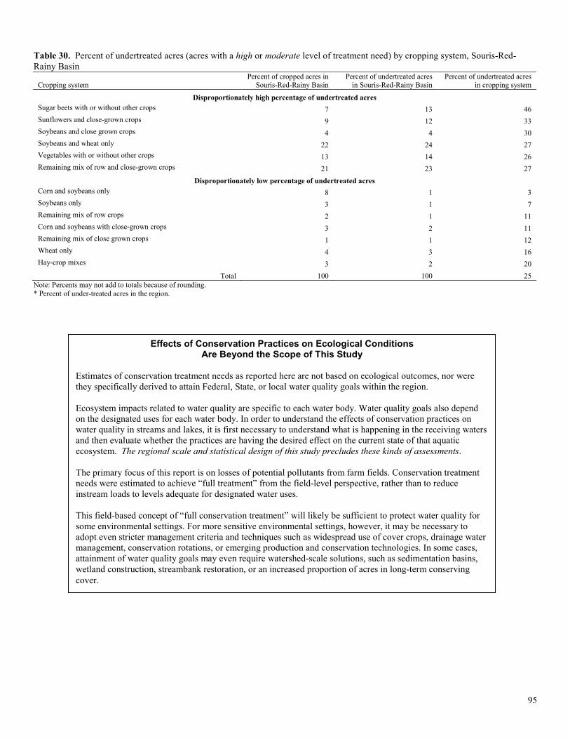
Table 30. Percent of undertreated acres (acres with a high or moderate level of treatment need) by cropping system, Souris-Red-Rainy Basin

Cropping system Percent of cropped acres in

Souris-Red-Rainy Basin Percent of undertreated acres

in Souris-Red-Rainy Basin Percent of undertreated acres

in cropping system

Disproportionately high percentage of undertreated acres Sugar beets with or without other crops 7 13 46 Sunflowers and close-grown crops 9 12 33 Soybeans and close grown crops 4 4 30 Soybeans and wheat only 22 24 27 Vegetables with or without other crops 13 14 26 Remaining mix of row and close-grown crops 21 23 27

Disproportionately low percentage of undertreated acres Corn and soybeans only 8 1 3 Soybeans only 3 1 7 Remaining mix of row crops 2 1 11 Corn and soybeans with close-grown crops 3 2 11 Remaining mix of close grown crops 1 1 12 Wheat only 4 3 16 Hay-crop mixes 3 2 20

Total 100 100 25 Note: Percents may not add to totals because of rounding. * Percent of under-treated acres in the region.

Effects of Conservation Practices on Ecological Conditions Are Beyond the Scope of This Study

Estimates of conservation treatment needs as reported here are not based on ecological outcomes, nor were they specifically derived to attain Federal, State, or local water quality goals within the region. Ecosystem impacts related to water quality are specific to each water body. Water quality goals also depend on the designated uses for each water body. In order to understand the effects of conservation practices on water quality in streams and lakes, it is first necessary to understand what is happening in the receiving waters and then evaluate whether the practices are having the desired effect on the current state of that aquatic ecosystem. The regional scale and statistical design of this study precludes these kinds of assessments. The primary focus of this report is on losses of potential pollutants from farm fields. Conservation treatment needs were estimated to achieve “full treatment” from the field-level perspective, rather than to reduce instream loads to levels adequate for designated water uses. This field-based concept of “full conservation treatment” will likely be sufficient to protect water quality for some environmental settings. For more sensitive environmental settings, however, it may be necessary to adopt even stricter management criteria and techniques such as widespread use of cover crops, drainage water management, conservation rotations, or emerging production and conservation technologies. In some cases, attainment of water quality goals may even require watershed-scale solutions, such as sedimentation basins, wetland construction, streambank restoration, or an increased proportion of acres in long-term conserving cover.

95

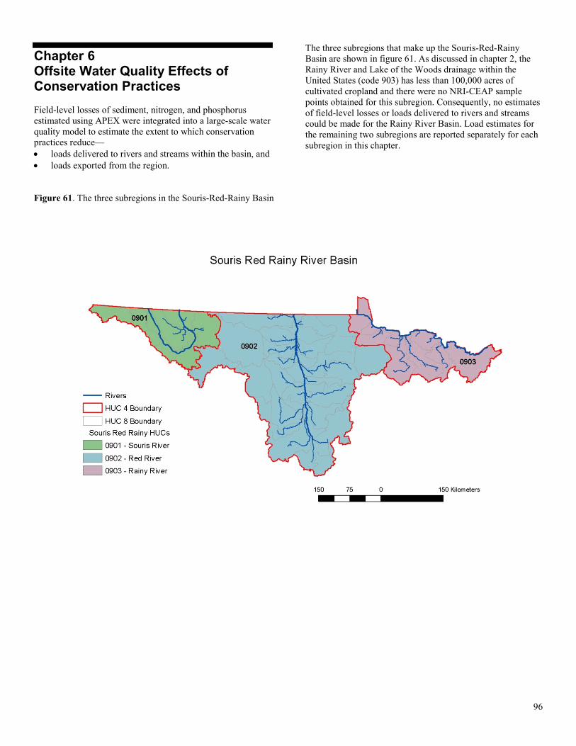
Chapter 6 Offsite Water Quality Effects of Conservation Practices Field-level losses of sediment, nitrogen, and phosphorus estimated using APEX were integrated into a large-scale water quality model to estimate the extent to which conservation practices reduce— • loads delivered to rivers and streams within the basin, and • loads exported from the region.

The three subregions that make up the Souris-Red-Rainy Basin are shown in figure 61. As discussed in chapter 2, the Rainy River and Lake of the Woods drainage within the United States (code 903) has less than 100,000 acres of cultivated cropland and there were no NRI-CEAP sample points obtained for this subregion. Consequently, no estimates of field-level losses or loads delivered to rivers and streams could be made for the Rainy River Basin. Load estimates for the remaining two subregions are reported separately for each subregion in this chapter.

Figure 61. The three subregions in the Souris-Red-Rainy Basin

96

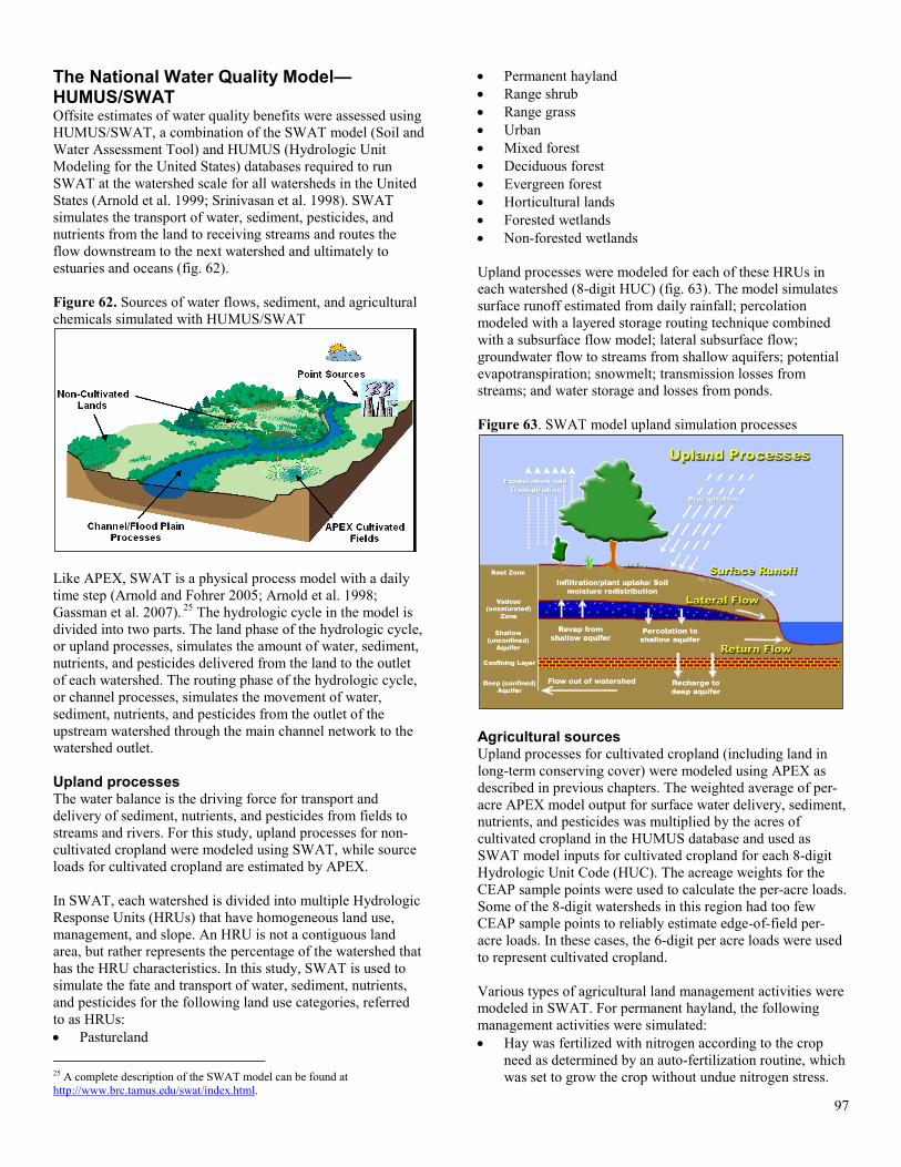
The National Water Quality Model—HUMUS/SWAT Offsite estimates of water quality benefits were assessed using HUMUS/SWAT, a combination of the SWAT model (Soil and Water Assessment Tool) and HUMUS (Hydrologic Unit Modeling for the United States) databases required to run SWAT at the watershed scale for all watersheds in the United States (Arnold et al. 1999; Srinivasan et al. 1998). SWAT simulates the transport of water, sediment, pesticides, and nutrients from the land to receiving streams and routes the flow downstream to the next watershed and ultimately to estuaries and oceans (fig. 62). Figure 62. Sources of water flows, sediment, and agricultural chemicals simulated with HUMUS/SWAT

Like APEX, SWAT is a physical process model with a daily time step (Arnold and Fohrer 2005; Arnold et al. 1998; Gassman et al. 2007).24F

25 The hydrologic cycle in the model is divided into two parts. The land phase of the hydrologic cycle, or upland processes, simulates the amount of water, sediment, nutrients, and pesticides delivered from the land to the outlet of each watershed. The routing phase of the hydrologic cycle, or channel processes, simulates the movement of water, sediment, nutrients, and pesticides from the outlet of the upstream watershed through the main channel network to the watershed outlet. Upland processes The water balance is the driving force for transport and delivery of sediment, nutrients, and pesticides from fields to streams and rivers. For this study, upland processes for non-cultivated cropland were modeled using SWAT, while source loads for cultivated cropland are estimated by APEX. In SWAT, each watershed is divided into multiple Hydrologic Response Units (HRUs) that have homogeneous land use, management, and slope. An HRU is not a contiguous land area, but rather represents the percentage of the watershed that has the HRU characteristics. In this study, SWAT is used to simulate the fate and transport of water, sediment, nutrients, and pesticides for the following land use categories, referred to as HRUs: • Pastureland

25 A complete description of the SWAT model can be found at http://www.brc.tamus.edu/swat/index.html.

• Permanent hayland • Range shrub • Range grass • Urban • Mixed forest • Deciduous forest • Evergreen forest • Horticultural lands • Forested wetlands • Non-forested wetlands Upland processes were modeled for each of these HRUs in each watershed (8-digit HUC) (fig. 63). The model simulates surface runoff estimated from daily rainfall; percolation modeled with a layered storage routing technique combined with a subsurface flow model; lateral subsurface flow; groundwater flow to streams from shallow aquifers; potential evapotranspiration; snowmelt; transmission losses from streams; and water storage and losses from ponds. Figure 63. SWAT model upland simulation processes

Agricultural sources Upland processes for cultivated cropland (including land in long-term conserving cover) were modeled using APEX as described in previous chapters. The weighted average of per-acre APEX model output for surface water delivery, sediment, nutrients, and pesticides was multiplied by the acres of cultivated cropland in the HUMUS database and used as SWAT model inputs for cultivated cropland for each 8-digit Hydrologic Unit Code (HUC). The acreage weights for the CEAP sample points were used to calculate the per-acre loads. Some of the 8-digit watersheds in this region had too few CEAP sample points to reliably estimate edge-of-field per-acre loads. In these cases, the 6-digit per acre loads were used to represent cultivated cropland. Various types of agricultural land management activities were modeled in SWAT. For permanent hayland, the following management activities were simulated: • Hay was fertilized with nitrogen according to the crop

need as determined by an auto-fertilization routine, which was set to grow the crop without undue nitrogen stress.

97

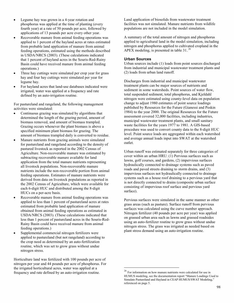
• Legume hay was grown in a 4-year rotation and

phosphorus was applied at the time of planting (every fourth year) at a rate of 50 pounds per acre, followed by applications of 13 pounds per acre every other year.

• Recoverable manure from animal feeding operations was applied to 1 percent of the hayland acres at rates estimated from probable land application of manure from animal feeding operations, estimated using the methods described in USDA/NRCS (2003). (These calculations indicated that 1 percent of hayland acres in the Souris-Red-Rainy Basin could have received manure from animal feeding operations.)

• Three hay cuttings were simulated per crop year for grass hay and four hay cuttings were simulated per year for legume hay.

• For hayland acres that land-use databases indicated were irrigated, water was applied at a frequency and rate defined by an auto-irrigation routine.

For pastureland and rangeland, the following management activities were simulated: • Continuous grazing was simulated by algorithms that

determined the length of the grazing period, amount of biomass removed, and amount of biomass trampled. Grazing occurs whenever the plant biomass is above a specified minimum plant biomass for grazing. The amount of biomass trampled daily is converted to residue.

• Manure nutrients from grazing animals were simulated for pastureland and rangeland according to the density of pastured livestock as reported in the 2002 Census of Agriculture. Non-recoverable manure was estimated by subtracting recoverable manure available for land application from the total manure nutrients representing all livestock populations. Non-recoverable manure nutrients include the non-recoverable portion from animal feeding operations. Estimates of manure nutrients were derived from data on livestock populations as reported in the 2002 Census of Agriculture, which were available for each 6-digit HUC and distributed among the 8-digit HUCs on a per-acre basis.

• Recoverable manure from animal feeding operations was applied to less than 1 percent of pastureland acres at rates estimated from probable land application of manure obtained from animal feeding operations as estimated in USDA/NRCS (2003). (These calculations indicated that less than 1 percent of pastureland acres in the Souris-Red-Rainy Basin could have received manure from animal feeding operations.)

• Supplemental commercial nitrogen fertilizers were applied to pastureland (but not rangeland) according to the crop need as determined by an auto-fertilization routine, which was set to grow grass without undue nitrogen stress.

Horticulture land was fertilized with 100 pounds per acre of nitrogen per year and 44 pounds per acre of phosphorus. For the irrigated horticultural acres, water was applied at a frequency and rate defined by an auto-irrigation routine.

Land application of biosolids from wastewater treatment facilities was not simulated. Manure nutrients from wildlife populations are not included in the model simulation. A summary of the total amount of nitrogen and phosphorus applied to agricultural land in the model simulation, including nitrogen and phosphorus applied to cultivated cropland in the APEX modeling, is presented in table 31.25F

26 Urban Sources Urban sources include (1) loads from point sources discharged from industrial and municipal wastewater treatment plants and (2) loads from urban land runoff. Discharges from industrial and municipal wastewater treatment plants can be major sources of nutrients and sediment in some watersheds. Point sources of water flow, total suspended sediment, total phosphorus, and Kjeldahl nitrogen were estimated using county-level data on population change to adjust 1980 estimates of point source loadings published by Resources for the Future (Gianessi and Peskin 1984) to the year 2000. The original Resources for the Future assessment covered 32,000 facilities, including industries, municipal wastewater treatment plants, and small sanitary waste facilities for the years 1977 to 1981. A GIS-based procedure was used to convert county data to the 8-digit HUC level. Point source loads are aggregated within each watershed and average annual loads input into SWAT at the watershed outlet. Urban runoff was estimated separately for three categories of cover within an urban HRU: (1) Pervious surfaces such as lawns, golf courses, and gardens, (2) impervious surfaces hydraulically connected to drainage systems such as paved roads and paved streets draining to storm drains, and (3) impervious surfaces not hydraulically connected to drainage systems such as a house roof draining to a pervious yard that is not directly connected to drains (composite urban surface consisting of impervious roof surface and pervious yard surface). Pervious surfaces were simulated in the same manner as other grass areas (such as pasture). Surface runoff from pervious surfaces was calculated using the curve number approach. Nitrogen fertilizer (40 pounds per acre per year) was applied on grassed urban area such as lawns and grassed roadsides using an auto-fertilizer routine to grow grass without undue nitrogen stress. The grass was irrigated as needed based on plant stress demand using an auto-irrigation routine.

26 For information on how manure nutrients were calculated for use in HUMUS modeling, see the documentation report “Manure Loadings Used to Simulate Pastureland and Hayland in CEAP HUMUS/SWAT Modeling,” referenced on page 5.

98

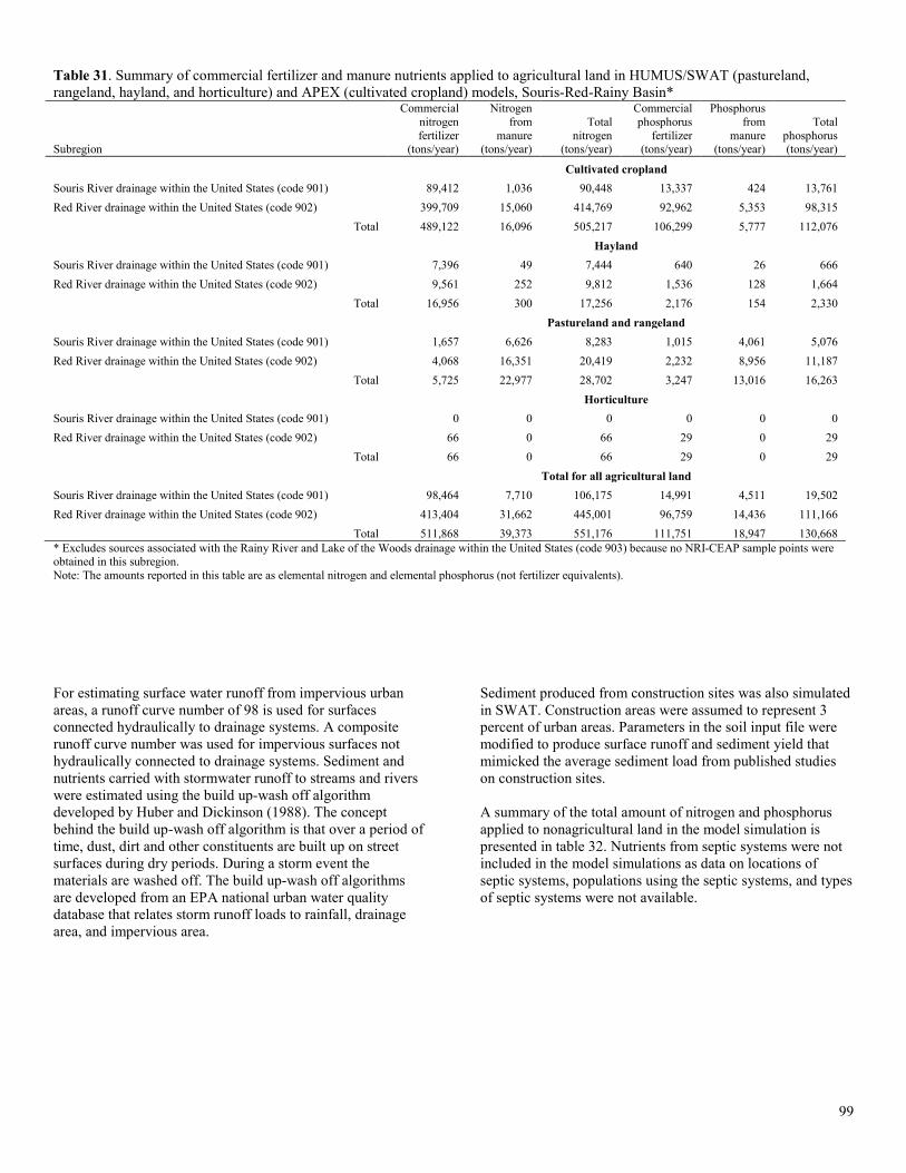
Table 31. Summary of commercial fertilizer and manure nutrients applied to agricultural land in HUMUS/SWAT (pastureland, rangeland, hayland, and horticulture) and APEX (cultivated cropland) models, Souris-Red-Rainy Basin*

Subregion

Commercial nitrogen fertilizer

(tons/year)

Nitrogen from

manure (tons/year)

Total nitrogen

(tons/year)

Commercial phosphorus

fertilizer (tons/year)

Phosphorus from

manure (tons/year)

Total phosphorus (tons/year)

Cultivated cropland Souris River drainage within the United States (code 901) 89,412 1,036 90,448 13,337 424 13,761 Red River drainage within the United States (code 902) 399,709 15,060 414,769 92,962 5,353 98,315

Total 489,122 16,096 505,217 106,299 5,777 112,076 Hayland Souris River drainage within the United States (code 901) 7,396 49 7,444 640 26 666 Red River drainage within the United States (code 902) 9,561 252 9,812 1,536 128 1,664

Total 16,956 300 17,256 2,176 154 2,330 Pastureland and rangeland Souris River drainage within the United States (code 901) 1,657 6,626 8,283 1,015 4,061 5,076 Red River drainage within the United States (code 902) 4,068 16,351 20,419 2,232 8,956 11,187

Total 5,725 22,977 28,702 3,247 13,016 16,263 Horticulture Souris River drainage within the United States (code 901) 0 0 0 0 0 0 Red River drainage within the United States (code 902) 66 0 66 29 0 29

Total 66 0 66 29 0 29 Total for all agricultural land Souris River drainage within the United States (code 901) 98,464 7,710 106,175 14,991 4,511 19,502 Red River drainage within the United States (code 902) 413,404 31,662 445,001 96,759 14,436 111,166

Total 511,868 39,373 551,176 111,751 18,947 130,668 * Excludes sources associated with the Rainy River and Lake of the Woods drainage within the United States (code 903) because no NRI-CEAP sample points were obtained in this subregion. Note: The amounts reported in this table are as elemental nitrogen and elemental phosphorus (not fertilizer equivalents). For estimating surface water runoff from impervious urban areas, a runoff curve number of 98 is used for surfaces connected hydraulically to drainage systems. A composite runoff curve number was used for impervious surfaces not hydraulically connected to drainage systems. Sediment and nutrients carried with stormwater runoff to streams and rivers were estimated using the build up-wash off algorithm developed by Huber and Dickinson (1988). The concept behind the build up-wash off algorithm is that over a period of time, dust, dirt and other constituents are built up on street surfaces during dry periods. During a storm event the materials are washed off. The build up-wash off algorithms are developed from an EPA national urban water quality database that relates storm runoff loads to rainfall, drainage area, and impervious area.

Sediment produced from construction sites was also simulated in SWAT. Construction areas were assumed to represent 3 percent of urban areas. Parameters in the soil input file were modified to produce surface runoff and sediment yield that mimicked the average sediment load from published studies on construction sites. A summary of the total amount of nitrogen and phosphorus applied to nonagricultural land in the model simulation is presented in table 32. Nutrients from septic systems were not included in the model simulations as data on locations of septic systems, populations using the septic systems, and types of septic systems were not available.

99

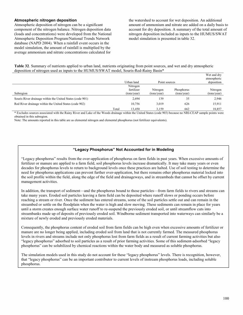
Atmospheric nitrogen deposition Atmospheric deposition of nitrogen can be a significant component of the nitrogen balance. Nitrogen deposition data (loads and concentrations) were developed from the National Atmospheric Deposition Program/National Trends Network database (NAPD 2004). When a rainfall event occurs in the model simulation, the amount of rainfall is multiplied by the average ammonium and nitrate concentrations calculated for

the watershed to account for wet deposition. An additional amount of ammonium and nitrate are added on a daily basis to account for dry deposition. A summary of the total amount of nitrogen deposition included as inputs to the HUMUS/SWAT model simulation is presented in table 32.

Table 32. Summary of nutrients applied to urban land, nutrients originating from point sources, and wet and dry atmospheric deposition of nitrogen used as inputs to the HUMUS/SWAT model, Souris-Red-Rainy Basin*

Urban land Point sources

Wet and dry atmospheric

deposition

Subregion

Nitrogen fertilizer

(tons/year) Nitrogen

(tons/year) Phosphorus (tons/year)

Nitrogen (tons/year)

Souris River drainage within the United States (code 901) 2,694 139 35 2,946 Red River drainage within the United States (code 902) 10,756 3,019 626 15,911

Total 13,450 3,159 662 18,857 * Excludes sources associated with the Rainy River and Lake of the Woods drainage within the United States (code 903) because no NRI-CEAP sample points were obtained in this subregion. Note: The amounts reported in this table are as elemental nitrogen and elemental phosphorus (not fertilizer equivalents). “Legacy Phosphorus” Not Accounted for in Modeling

“Legacy phosphorus” results from the over-application of phosphorus on farm fields in past years. When excessive amounts of fertilizer or manure are applied to a farm field, soil phosphorus levels increase dramatically. It may take many years or even decades for phosphorus levels to return to background levels once these practices are halted. Use of soil testing to determine the need for phosphorus applications can prevent further over-application, but there remains other phosphorus material locked into the soil profile within the field, along the edge of the field and drainageways, and in streambeds that cannot be offset by current management activities. In addition, the transport of sediment—and the phosphorus bound to those particles—from farm fields to rivers and streams can take many years. Eroded soil particles leaving a farm field can be deposited where runoff slows or ponding occurs before reaching a stream or river. Once the sediment has entered streams, some of the soil particles settle out and can remain in the streambed or settle on the floodplain when the water is high and slow moving. These sediments can remain in place for years until a storm creates enough surface water runoff to re-suspend the previously eroded soil, or until streamflow cuts into streambanks made up of deposits of previously eroded soil. Windborne sediment transported into waterways can similarly be a mixture of newly eroded and previously eroded materials. Consequently, the phosphorus content of eroded soil from farm fields can be high even when excessive amounts of fertilizer or manure are no longer being applied, including eroded soil from land that is not currently farmed. The measured phosphorus levels in rivers and streams include not only phosphorus lost from farm fields as a result of current farming activities but also “legacy phosphorus” adsorbed to soil particles as a result of prior farming activities. Some of this sediment-adsorbed “legacy phosphorus” can be solubilized by chemical reactions within the water body and measured as soluble phosphorus. The simulation models used in this study do not account for these “legacy phosphorus” levels. There is recognition, however, that “legacy phosphorus” can be an important contributor to current levels of instream phosphorus loads, including soluble phosphorus.

100

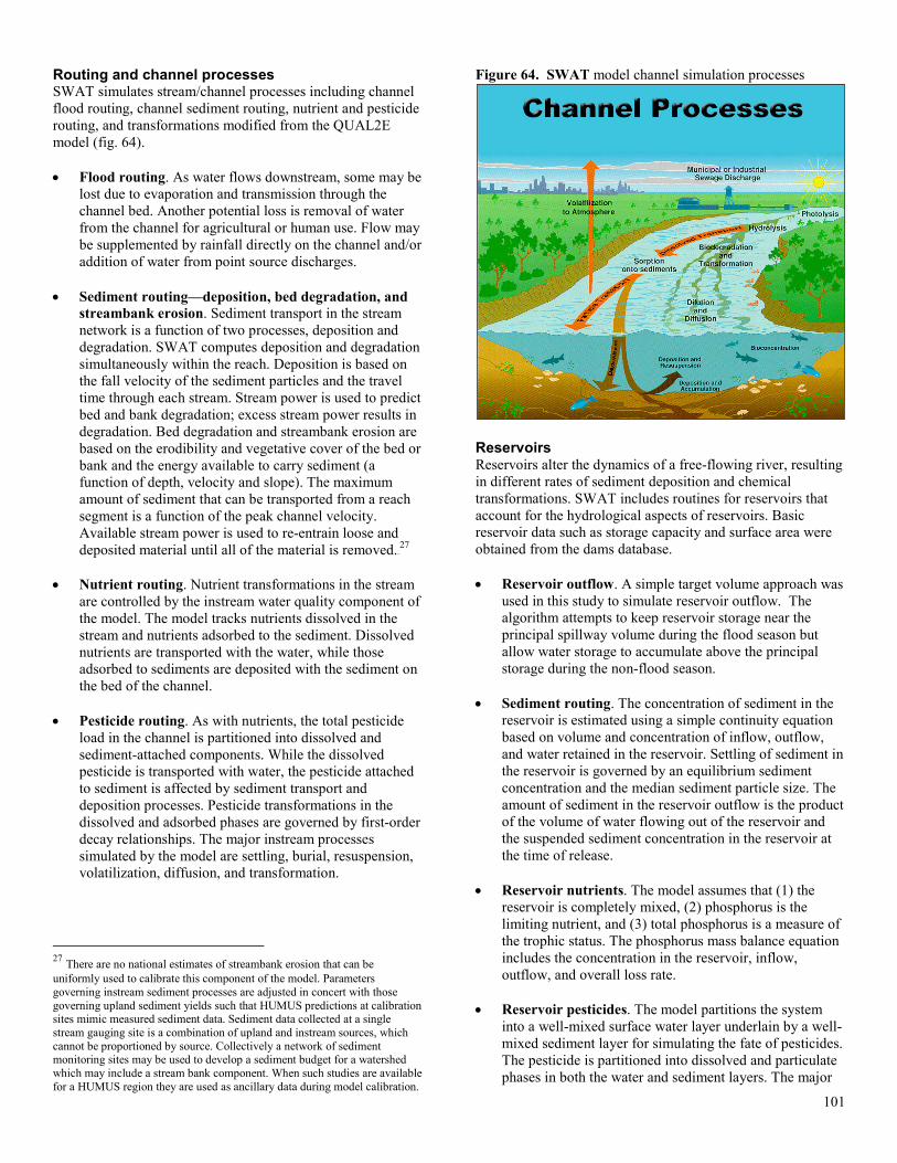
Routing and channel processes SWAT simulates stream/channel processes including channel flood routing, channel sediment routing, nutrient and pesticide routing, and transformations modified from the QUAL2E model (fig. 64). • Flood routing. As water flows downstream, some may be

lost due to evaporation and transmission through the channel bed. Another potential loss is removal of water from the channel for agricultural or human use. Flow may be supplemented by rainfall directly on the channel and/or addition of water from point source discharges.

• Sediment routing—deposition, bed degradation, and

streambank erosion. Sediment transport in the stream network is a function of two processes, deposition and degradation. SWAT computes deposition and degradation simultaneously within the reach. Deposition is based on the fall velocity of the sediment particles and the travel time through each stream. Stream power is used to predict bed and bank degradation; excess stream power results in degradation. Bed degradation and streambank erosion are based on the erodibility and vegetative cover of the bed or bank and the energy available to carry sediment (a function of depth, velocity and slope). The maximum amount of sediment that can be transported from a reach segment is a function of the peak channel velocity. Available stream power is used to re-entrain loose and deposited material until all of the material is removed.26F

27 • Nutrient routing. Nutrient transformations in the stream

are controlled by the instream water quality component of the model. The model tracks nutrients dissolved in the stream and nutrients adsorbed to the sediment. Dissolved nutrients are transported with the water, while those adsorbed to sediments are deposited with the sediment on the bed of the channel.

• Pesticide routing. As with nutrients, the total pesticide

load in the channel is partitioned into dissolved and sediment-attached components. While the dissolved pesticide is transported with water, the pesticide attached to sediment is affected by sediment transport and deposition processes. Pesticide transformations in the dissolved and adsorbed phases are governed by first-order decay relationships. The major instream processes simulated by the model are settling, burial, resuspension, volatilization, diffusion, and transformation.

27 There are no national estimates of streambank erosion that can be uniformly used to calibrate this component of the model. Parameters governing instream sediment processes are adjusted in concert with those governing upland sediment yields such that HUMUS predictions at calibration sites mimic measured sediment data. Sediment data collected at a single stream gauging site is a combination of upland and instream sources, which cannot be proportioned by source. Collectively a network of sediment monitoring sites may be used to develop a sediment budget for a watershed which may include a stream bank component. When such studies are available for a HUMUS region they are used as ancillary data during model calibration.

Figure 64. SWAT model channel simulation processes

Reservoirs Reservoirs alter the dynamics of a free-flowing river, resulting in different rates of sediment deposition and chemical transformations. SWAT includes routines for reservoirs that account for the hydrological aspects of reservoirs. Basic reservoir data such as storage capacity and surface area were obtained from the dams database. • Reservoir outflow. A simple target volume approach was

used in this study to simulate reservoir outflow. The algorithm attempts to keep reservoir storage near the principal spillway volume during the flood season but allow water storage to accumulate above the principal storage during the non-flood season.

• Sediment routing. The concentration of sediment in the

reservoir is estimated using a simple continuity equation based on volume and concentration of inflow, outflow, and water retained in the reservoir. Settling of sediment in the reservoir is governed by an equilibrium sediment concentration and the median sediment particle size. The amount of sediment in the reservoir outflow is the product of the volume of water flowing out of the reservoir and the suspended sediment concentration in the reservoir at the time of release.

• Reservoir nutrients. The model assumes that (1) the

reservoir is completely mixed, (2) phosphorus is the limiting nutrient, and (3) total phosphorus is a measure of the trophic status. The phosphorus mass balance equation includes the concentration in the reservoir, inflow, outflow, and overall loss rate.

• Reservoir pesticides. The model partitions the system

into a well-mixed surface water layer underlain by a well-mixed sediment layer for simulating the fate of pesticides. The pesticide is partitioned into dissolved and particulate phases in both the water and sediment layers. The major

101

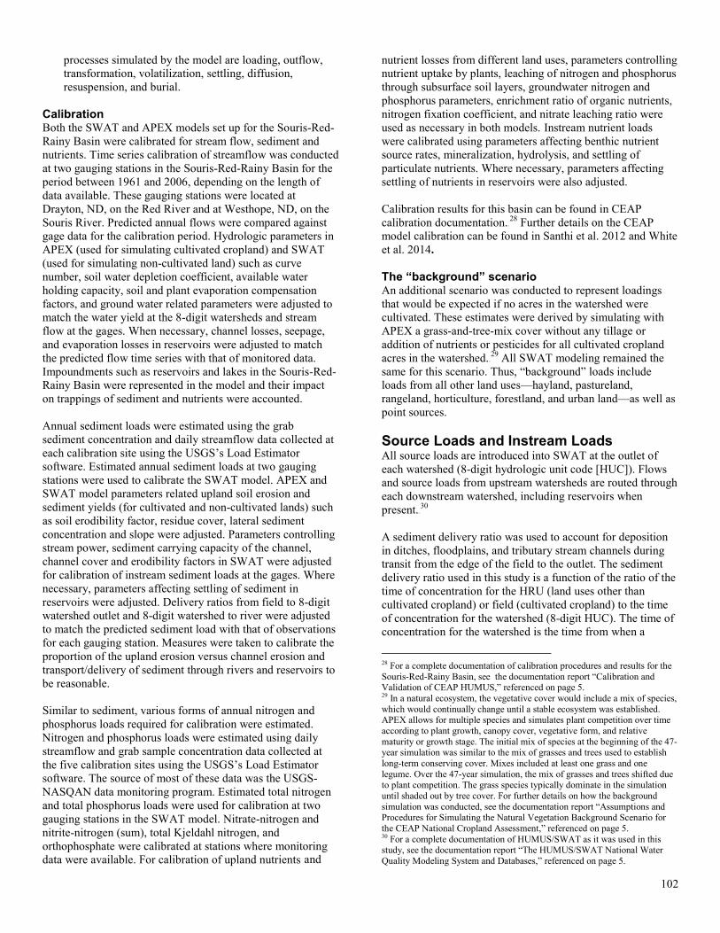
processes simulated by the model are loading, outflow, transformation, volatilization, settling, diffusion, resuspension, and burial.

Calibration Both the SWAT and APEX models set up for the Souris-Red-Rainy Basin were calibrated for stream flow, sediment and nutrients. Time series calibration of streamflow was conducted at two gauging stations in the Souris-Red-Rainy Basin for the period between 1961 and 2006, depending on the length of data available. These gauging stations were located at Drayton, ND, on the Red River and at Westhope, ND, on the Souris River. Predicted annual flows were compared against gage data for the calibration period. Hydrologic parameters in APEX (used for simulating cultivated cropland) and SWAT (used for simulating non-cultivated land) such as curve number, soil water depletion coefficient, available water holding capacity, soil and plant evaporation compensation factors, and ground water related parameters were adjusted to match the water yield at the 8-digit watersheds and stream flow at the gages. When necessary, channel losses, seepage, and evaporation losses in reservoirs were adjusted to match the predicted flow time series with that of monitored data. Impoundments such as reservoirs and lakes in the Souris-Red-Rainy Basin were represented in the model and their impact on trappings of sediment and nutrients were accounted. Annual sediment loads were estimated using the grab sediment concentration and daily streamflow data collected at each calibration site using the USGS’s Load Estimator software. Estimated annual sediment loads at two gauging stations were used to calibrate the SWAT model. APEX and SWAT model parameters related upland soil erosion and sediment yields (for cultivated and non-cultivated lands) such as soil erodibility factor, residue cover, lateral sediment concentration and slope were adjusted. Parameters controlling stream power, sediment carrying capacity of the channel, channel cover and erodibility factors in SWAT were adjusted for calibration of instream sediment loads at the gages. Where necessary, parameters affecting settling of sediment in reservoirs were adjusted. Delivery ratios from field to 8-digit watershed outlet and 8-digit watershed to river were adjusted to match the predicted sediment load with that of observations for each gauging station. Measures were taken to calibrate the proportion of the upland erosion versus channel erosion and transport/delivery of sediment through rivers and reservoirs to be reasonable. Similar to sediment, various forms of annual nitrogen and phosphorus loads required for calibration were estimated. Nitrogen and phosphorus loads were estimated using daily streamflow and grab sample concentration data collected at the five calibration sites using the USGS’s Load Estimator software. The source of most of these data was the USGS-NASQAN data monitoring program. Estimated total nitrogen and total phosphorus loads were used for calibration at two gauging stations in the SWAT model. Nitrate-nitrogen and nitrite-nitrogen (sum), total Kjeldahl nitrogen, and orthophosphate were calibrated at stations where monitoring data were available. For calibration of upland nutrients and

nutrient losses from different land uses, parameters controlling nutrient uptake by plants, leaching of nitrogen and phosphorus through subsurface soil layers, groundwater nitrogen and phosphorus parameters, enrichment ratio of organic nutrients, nitrogen fixation coefficient, and nitrate leaching ratio were used as necessary in both models. Instream nutrient loads were calibrated using parameters affecting benthic nutrient source rates, mineralization, hydrolysis, and settling of particulate nutrients. Where necessary, parameters affecting settling of nutrients in reservoirs were also adjusted. Calibration results for this basin can be found in CEAP calibration documentation.27F

28 Further details on the CEAP model calibration can be found in Santhi et al. 2012 and White et al. 2014. The “background” scenario An additional scenario was conducted to represent loadings that would be expected if no acres in the watershed were cultivated. These estimates were derived by simulating with APEX a grass-and-tree-mix cover without any tillage or addition of nutrients or pesticides for all cultivated cropland acres in the watershed.28F

29 All SWAT modeling remained the same for this scenario. Thus, “background” loads include loads from all other land uses—hayland, pastureland, rangeland, horticulture, forestland, and urban land—as well as point sources. Source Loads and Instream Loads All source loads are introduced into SWAT at the outlet of each watershed (8-digit hydrologic unit code [HUC]). Flows and source loads from upstream watersheds are routed through each downstream watershed, including reservoirs when present.29F

30 A sediment delivery ratio was used to account for deposition in ditches, floodplains, and tributary stream channels during transit from the edge of the field to the outlet. The sediment delivery ratio used in this study is a function of the ratio of the time of concentration for the HRU (land uses other than cultivated cropland) or field (cultivated cropland) to the time of concentration for the watershed (8-digit HUC). The time of concentration for the watershed is the time from when a

28 For a complete documentation of calibration procedures and results for the Souris-Red-Rainy Basin, see the documentation report “Calibration and Validation of CEAP HUMUS,” referenced on page 5. 29 In a natural ecosystem, the vegetative cover would include a mix of species, which would continually change until a stable ecosystem was established. APEX allows for multiple species and simulates plant competition over time according to plant growth, canopy cover, vegetative form, and relative maturity or growth stage. The initial mix of species at the beginning of the 47-year simulation was similar to the mix of grasses and trees used to establish long-term conserving cover. Mixes included at least one grass and one legume. Over the 47-year simulation, the mix of grasses and trees shifted due to plant competition. The grass species typically dominate in the simulation until shaded out by tree cover. For further details on how the background simulation was conducted, see the documentation report “Assumptions and Procedures for Simulating the Natural Vegetation Background Scenario for the CEAP National Cropland Assessment,” referenced on page 5. 30 For a complete documentation of HUMUS/SWAT as it was used in this study, see the documentation report “The HUMUS/SWAT National Water Quality Modeling System and Databases,” referenced on page 5.

102

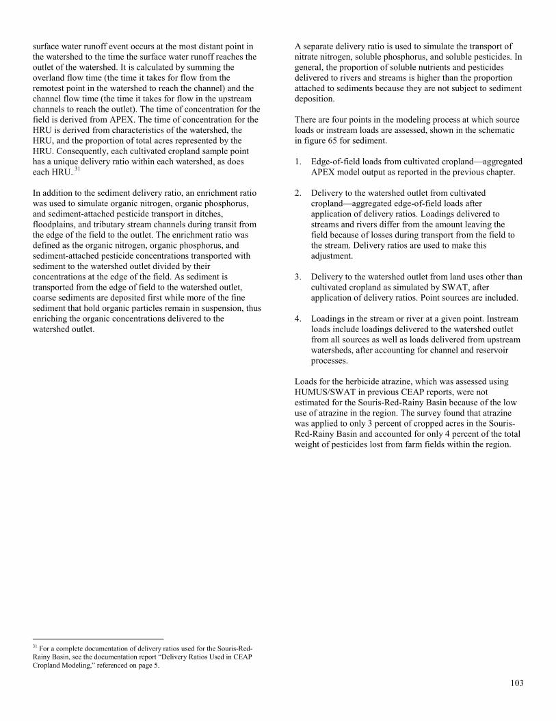
surface water runoff event occurs at the most distant point in the watershed to the time the surface water runoff reaches the outlet of the watershed. It is calculated by summing the overland flow time (the time it takes for flow from the remotest point in the watershed to reach the channel) and the channel flow time (the time it takes for flow in the upstream channels to reach the outlet). The time of concentration for the field is derived from APEX. The time of concentration for the HRU is derived from characteristics of the watershed, the HRU, and the proportion of total acres represented by the HRU. Consequently, each cultivated cropland sample point has a unique delivery ratio within each watershed, as does each HRU.30F

31 In addition to the sediment delivery ratio, an enrichment ratio was used to simulate organic nitrogen, organic phosphorus, and sediment-attached pesticide transport in ditches, floodplains, and tributary stream channels during transit from the edge of the field to the outlet. The enrichment ratio was defined as the organic nitrogen, organic phosphorus, and sediment-attached pesticide concentrations transported with sediment to the watershed outlet divided by their concentrations at the edge of the field. As sediment is transported from the edge of field to the watershed outlet, coarse sediments are deposited first while more of the fine sediment that hold organic particles remain in suspension, thus enriching the organic concentrations delivered to the watershed outlet.

31 For a complete documentation of delivery ratios used for the Souris-Red-Rainy Basin, see the documentation report “Delivery Ratios Used in CEAP Cropland Modeling,” referenced on page 5.

A separate delivery ratio is used to simulate the transport of nitrate nitrogen, soluble phosphorus, and soluble pesticides. In general, the proportion of soluble nutrients and pesticides delivered to rivers and streams is higher than the proportion attached to sediments because they are not subject to sediment deposition. There are four points in the modeling process at which source loads or instream loads are assessed, shown in the schematic in figure 65 for sediment. 1. Edge-of-field loads from cultivated cropland—aggregated

APEX model output as reported in the previous chapter. 2. Delivery to the watershed outlet from cultivated

cropland—aggregated edge-of-field loads after application of delivery ratios. Loadings delivered to streams and rivers differ from the amount leaving the field because of losses during transport from the field to the stream. Delivery ratios are used to make this adjustment.

3. Delivery to the watershed outlet from land uses other than

cultivated cropland as simulated by SWAT, after application of delivery ratios. Point sources are included.

4. Loadings in the stream or river at a given point. Instream

loads include loadings delivered to the watershed outlet from all sources as well as loads delivered from upstream watersheds, after accounting for channel and reservoir processes.

Loads for the herbicide atrazine, which was assessed using HUMUS/SWAT in previous CEAP reports, were not estimated for the Souris-Red-Rainy Basin because of the low use of atrazine in the region. The survey found that atrazine was applied to only 3 percent of cropped acres in the Souris-Red-Rainy Basin and accounted for only 4 percent of the total weight of pesticides lost from farm fields within the region.

103

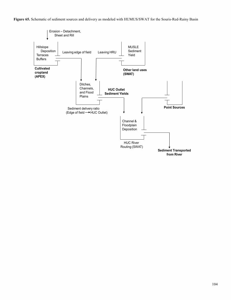
Figure 65. Schematic of sediment sources and delivery as modeled with HUMUS/SWAT for the Souris-Red-Rainy Basin

Erosion – Detachment,Sheet and Rill

HillslopeDeposition

TerracesBuffers

Sediment delivery ratio(Edge of field HUC Outlet)

MUSLESedimentYield

Leaving edge of field Leaving HRU

Other land uses (SWAT)

Ditches,Channels,and FloodPlains

Cultivated cropland (APEX)

HUC Outlet Sediment Yields

Point Sources

Channel &Floodplain Deposition

HUC RiverRouting (SWAT)

Sediment Transportedfrom River

104

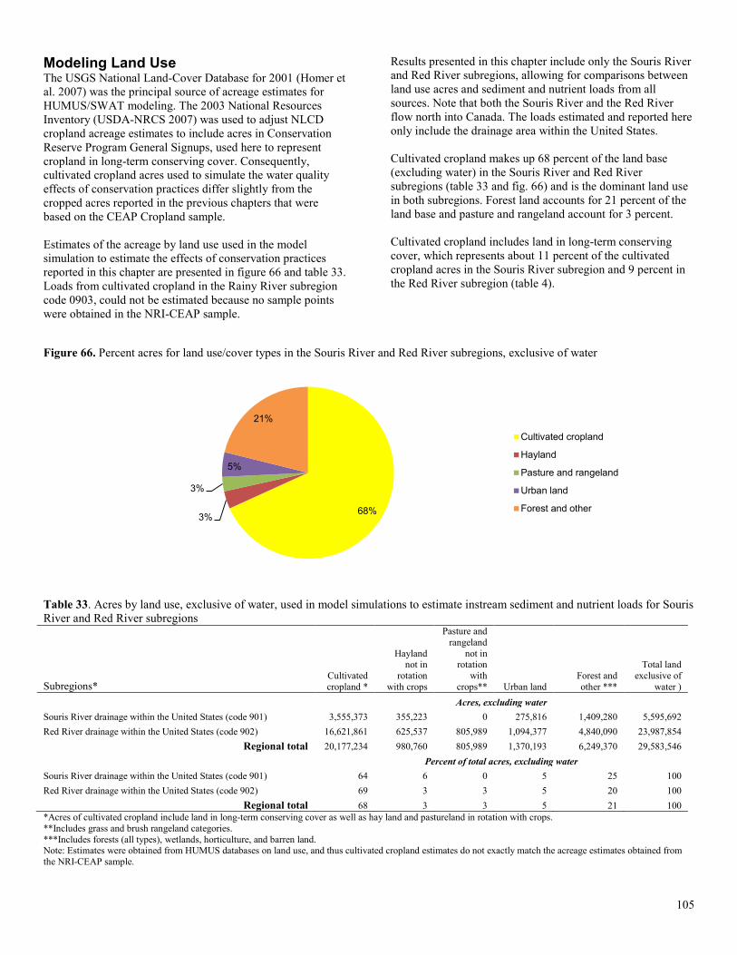
Modeling Land Use The USGS National Land-Cover Database for 2001 (Homer et al. 2007) was the principal source of acreage estimates for HUMUS/SWAT modeling. The 2003 National Resources Inventory (USDA-NRCS 2007) was used to adjust NLCD cropland acreage estimates to include acres in Conservation Reserve Program General Signups, used here to represent cropland in long-term conserving cover. Consequently, cultivated cropland acres used to simulate the water quality effects of conservation practices differ slightly from the cropped acres reported in the previous chapters that were based on the CEAP Cropland sample. Estimates of the acreage by land use used in the model simulation to estimate the effects of conservation practices reported in this chapter are presented in figure 66 and table 33. Loads from cultivated cropland in the Rainy River subregion code 0903, could not be estimated because no sample points were obtained in the NRI-CEAP sample.

Results presented in this chapter include only the Souris River and Red River subregions, allowing for comparisons between land use acres and sediment and nutrient loads from all sources. Note that both the Souris River and the Red River flow north into Canada. The loads estimated and reported here only include the drainage area within the United States. Cultivated cropland makes up 68 percent of the land base (excluding water) in the Souris River and Red River subregions (table 33 and fig. 66) and is the dominant land use in both subregions. Forest land accounts for 21 percent of the land base and pasture and rangeland account for 3 percent. Cultivated cropland includes land in long-term conserving cover, which represents about 11 percent of the cultivated cropland acres in the Souris River subregion and 9 percent in the Red River subregion (table 4).

Figure 66. Percent acres for land use/cover types in the Souris River and Red River subregions, exclusive of water

Table 33. Acres by land use, exclusive of water, used in model simulations to estimate instream sediment and nutrient loads for Souris River and Red River subregions

Subregions* Cultivated cropland *

Hayland not in

rotation with crops

Pasture and rangeland

not in rotation

with crops** Urban land

Forest and other ***

Total land exclusive of

water ) Acres, excluding water Souris River drainage within the United States (code 901) 3,555,373 355,223 0 275,816 1,409,280 5,595,692 Red River drainage within the United States (code 902) 16,621,861 625,537 805,989 1,094,377 4,840,090 23,987,854

Regional total 20,177,234 980,760 805,989 1,370,193 6,249,370 29,583,546 Percent of total acres, excluding water Souris River drainage within the United States (code 901) 64 6 0 5 25 100 Red River drainage within the United States (code 902) 69 3 3 5 20 100

Regional total 68 3 3 5 21 100 *Acres of cultivated cropland include land in long-term conserving cover as well as hay land and pastureland in rotation with crops. **Includes grass and brush rangeland categories. ***Includes forests (all types), wetlands, horticulture, and barren land. Note: Estimates were obtained from HUMUS databases on land use, and thus cultivated cropland estimates do not exactly match the acreage estimates obtained from the NRI-CEAP sample.

68% 3%

3%

5%

21%

Cultivated cropland

Hayland

Pasture and rangeland

Urban land

Forest and other

105

Loads Delivered from Cultivated Cropland to Rivers and Streams within the Region HUMUS/SWAT accounts for the transport of water, sediment, pesticides, and nutrients from the land to receiving streams and routes the flow downstream to the next watershed and ultimately to estuaries and oceans. Not all of the sediment, nutrients, and pesticides that leave farm fields are delivered to streams and rivers. Some material is bound up in various parts of the landscape during transport. Loads delivered from cultivated cropland and other sources to rivers and streams within the region are presented in this section. The water quality effects of conservation practices in use during 2003–06 on loads delivered from cultivated cropland to rivers and streams were assessed by comparing HUMUS/SWAT model simulation results for the baseline conservation condition to simulation results for the no-practice scenario. For the no-practice scenario, only the conditions for cultivated cropland were changed, as described previously. All other aspects of the simulations—including sediment and nutrient loads from point sources and land uses other than cultivated cropland—remained the same.

In summary, findings for the Souris and Red Rivers indicate that for the baseline conservation condition, sediment and nutrient loads delivered to rivers and streams from cultivated cropland sources per year, on average, are: • 371,000 tons of sediment (77 percent of loads from all

sources); • 53.3 million pounds of nitrogen (83 percent of loads from

all sources); and • 2.1 million pounds of phosphorus (57 percent of loads

from all sources). Conservation practices in use on cultivated cropland in 2003-06, including land in long-term conserving cover, have reduced sediment and nutrient loads delivered to rivers and streams from cultivated cropland sources per year, on average, by: • 50 percent for sediment; • 75 percent for nitrogen; and • 52 percent for phosphorus.

106

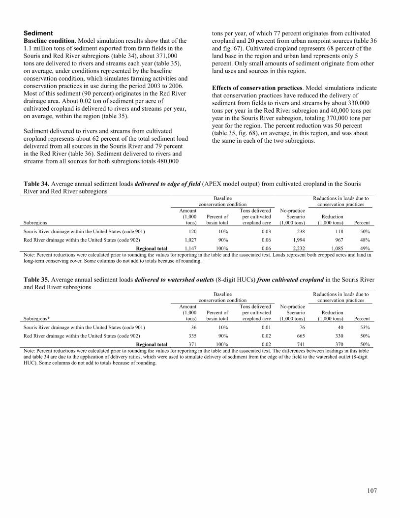
Sediment Baseline condition. Model simulation results show that of the 1.1 million tons of sediment exported from farm fields in the Souris and Red River subregions (table 34), about 371,000 tons are delivered to rivers and streams each year (table 35), on average, under conditions represented by the baseline conservation condition, which simulates farming activities and conservation practices in use during the period 2003 to 2006. Most of this sediment (90 percent) originates in the Red River drainage area. About 0.02 ton of sediment per acre of cultivated cropland is delivered to rivers and streams per year, on average, within the region (table 35). Sediment delivered to rivers and streams from cultivated cropland represents about 62 percent of the total sediment load delivered from all sources in the Souris River and 79 percent in the Red River (table 36). Sediment delivered to rivers and streams from all sources for both subregions totals 480,000

tons per year, of which 77 percent originates from cultivated cropland and 20 percent from urban nonpoint sources (table 36 and fig. 67). Cultivated cropland represents 68 percent of the land base in the region and urban land represents only 5 percent. Only small amounts of sediment originate from other land uses and sources in this region. Effects of conservation practices. Model simulations indicate that conservation practices have reduced the delivery of sediment from fields to rivers and streams by about 330,000 tons per year in the Red River subregion and 40,000 tons per year in the Souris River subregion, totaling 370,000 tons per year for the region. The percent reduction was 50 percent (table 35, fig. 68), on average, in this region, and was about the same in each of the two subregions.

Table 34. Average annual sediment loads delivered to edge of field (APEX model output) from cultivated cropland in the Souris River and Red River subregions

Baseline

conservation condition Reductions in loads due to

conservation practices

Subregions

Amount (1,000

tons) Percent of basin total

Tons delivered per cultivated cropland acre

No-practice Scenario

(1,000 tons) Reduction

(1,000 tons) Percent

Souris River drainage within the United States (code 901) 120 10% 0.03 238 118 50% Red River drainage within the United States (code 902) 1,027 90% 0.06 1,994 967 48%

Regional total 1,147 100% 0.06 2,232 1,085 49% Note: Percent reductions were calculated prior to rounding the values for reporting in the table and the associated text. Loads represent both cropped acres and land in long-term conserving cover. Some columns do not add to totals because of rounding. Table 35. Average annual sediment loads delivered to watershed outlets (8-digit HUCs) from cultivated cropland in the Souris River and Red River subregions

Baseline

conservation condition Reductions in loads due to

conservation practices

Subregions*

Amount (1,000

tons) Percent of basin total

Tons delivered per cultivated cropland acre

No-practice Scenario

(1,000 tons) Reduction

(1,000 tons) Percent

Souris River drainage within the United States (code 901) 36 10% 0.01 76 40 53% Red River drainage within the United States (code 902) 335 90% 0.02 665 330 50%

Regional total 371 100% 0.02 741 370 50% Note: Percent reductions were calculated prior to rounding the values for reporting in the table and the associated text. The differences between loadings in this table and table 34 are due to the application of delivery ratios, which were used to simulate delivery of sediment from the edge of the field to the watershed outlet (8-digit HUC). Some columns do not add to totals because of rounding.

107

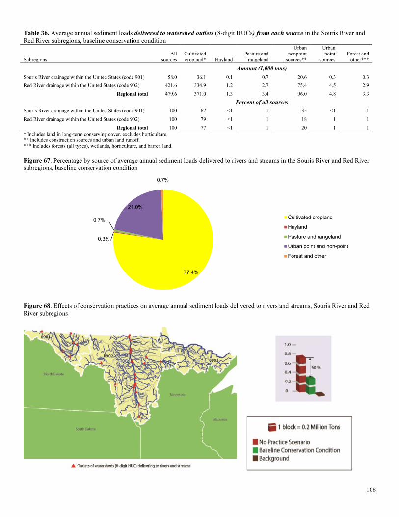
Table 36. Average annual sediment loads delivered to watershed outlets (8-digit HUCs) from each source in the Souris River and Red River subregions, baseline conservation condition

Subregions All

sources Cultivated cropland* Hayland

Pasture and rangeland

Urban nonpoint

sources**

Urban point

sources Forest and

other***

Amount (1,000 tons) Souris River drainage within the United States (code 901) 58.0 36.1 0.1 0.7 20.6 0.3 0.3 Red River drainage within the United States (code 902) 421.6 334.9 1.2 2.7 75.4 4.5 2.9

Regional total 479.6 371.0 1.3 3.4 96.0 4.8 3.3 Percent of all sources Souris River drainage within the United States (code 901) 100 62 <1 1 35 <1 1 Red River drainage within the United States (code 902) 100 79 <1 1 18 1 1

Regional total 100 77 <1 1 20 1 1 * Includes land in long-term conserving cover, excludes horticulture. ** Includes construction sources and urban land runoff. *** Includes forests (all types), wetlands, horticulture, and barren land. Figure 67. Percentage by source of average annual sediment loads delivered to rivers and streams in the Souris River and Red River subregions, baseline conservation condition

Figure 68. Effects of conservation practices on average annual sediment loads delivered to rivers and streams, Souris River and Red River subregions

77.4%

0.3%

0.7%

21.0%

0.7%

Cultivated cropland

Hayland

Pasture and rangeland

Urban point and non-point

Forest and other

108

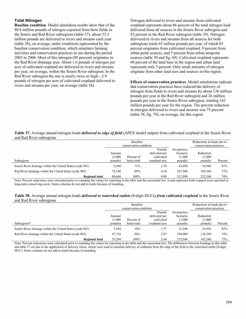
Total Nitrogen Baseline condition. Model simulation results show that of the 80.6 million pounds of nitrogen exported from farm fields in the Souris and Red River subregions (table 37), about 53.3 million pounds are delivered to rivers and streams each year (table 38), on average, under conditions represented by the baseline conservation condition, which simulates farming activities and conservation practices in use during the period 2003 to 2006. Most of this nitrogen (90 percent) originates in the Red River drainage area. About 1.6 pounds of nitrogen per acre of cultivated cropland are delivered to rivers and streams per year, on average, within the Souris River subregion. In the Red River subregion the rate is nearly twice as high—2.9 pounds of nitrogen per acre of cultivated cropland delivered to rivers and streams per year, on average (table 38).

Nitrogen delivered to rivers and streams from cultivated cropland represents about 86 percent of the total nitrogen load delivered from all sources in the Souris River subregion and 82 percent in the Red River subregion (table 39). Nitrogen delivered to rivers and streams from all sources for both subregions totals 65 million pounds per year, of which 83 percent originates from cultivated cropland, 9 percent from urban point sources, and 5 percent from urban nonpoint sources (table 39 and fig. 69). Cultivated cropland represents 68 percent of the land base in the region and urban land represents only 5 percent. Only small amounts of nitrogen originate from other land uses and sources in this region. Effects of conservation practices. Model simulations indicate that conservation practices have reduced the delivery of nitrogen from fields to rivers and streams by about 136 million pounds per year in the Red River subregion and 26 million pounds per year in the Souris River subregion, totaling 162 million pounds per year for the region. The percent reduction in nitrogen delivered to rivers and streams was 75 percent (table 38, fig. 70), on average, for this region.

Table 37. Average annual nitrogen loads delivered to edge of field (APEX model output) from cultivated cropland in the Souris River and Red River subregions

Baseline

conservation condition Reductions in loads due to

conservation practices

Subregions

Amount (1,000

pounds) Percent of basin total

Pounds delivered per

cultivated cropland acre

No-practice Scenario

(1,000 pounds)

Reduction (1,000

pounds) Percent

Souris River drainage within the United States (code 901) 8,504 11% 2.39 45,490 36,986 81% Red River drainage within the United States (code 902) 72,140 89% 4.34 267,500 195,360 73%

Regional total 80,644 100% 4.00 312,990 232,346 74% Note: Percent reductions were calculated prior to rounding the values for reporting in the table and the associated text. Loads represent both cropped acres and land in long-term conserving cover. Some columns do not add to totals because of rounding. Table 38. Average annual nitrogen loads delivered to watershed outlets (8-digit HUCs) from cultivated cropland in the Souris River and Red River subregions

Baseline

conservation condition Reductions in loads due to

conservation practices

Subregions*

Amount (1,000

pounds) Percent of basin total

Pounds delivered per

cultivated cropland acre

No-practice Scenario

(1,000 pounds)

Reduction (1,000

pounds) Percent

Souris River drainage within the United States (code 901) 5,584 10% 1.57 31,540 25,956 82% Red River drainage within the United States (code 902) 47,710 90% 2.87 184,000 136,290 74%

Regional total 53,294 100% 2.64 215,540 162,246 75% Note: Percent reductions were calculated prior to rounding the values for reporting in the table and the associated text. The differences between loadings in this table and table 37 are due to the application of delivery ratios, which were used to simulate delivery of sediment from the edge of the field to the watershed outlet (8-digit HUC). Some columns do not add to totals because of rounding.

109

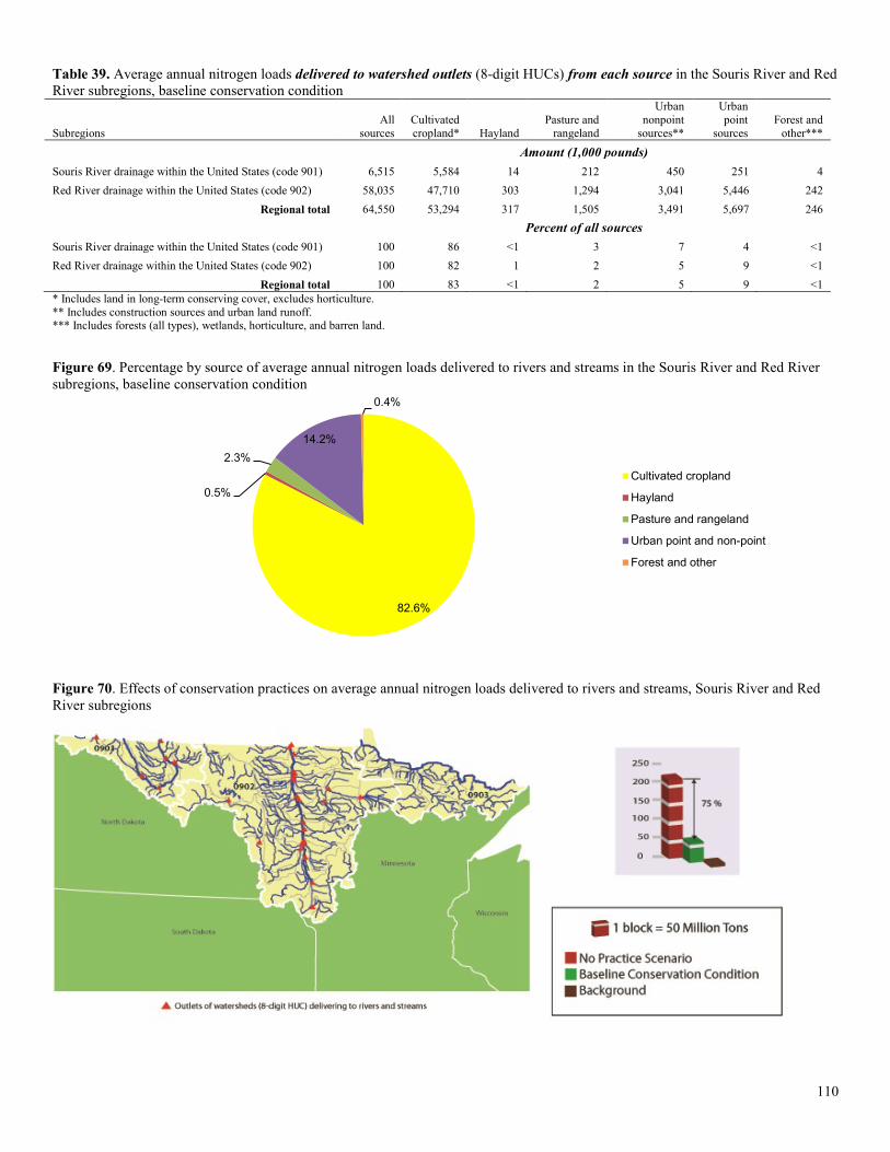
Table 39. Average annual nitrogen loads delivered to watershed outlets (8-digit HUCs) from each source in the Souris River and Red River subregions, baseline conservation condition

Subregions All

sources Cultivated cropland* Hayland

Pasture and rangeland

Urban nonpoint

sources**

Urban point

sources Forest and

other***

Amount (1,000 pounds) Souris River drainage within the United States (code 901) 6,515 5,584 14 212 450 251 4 Red River drainage within the United States (code 902) 58,035 47,710 303 1,294 3,041 5,446 242

Regional total 64,550 53,294 317 1,505 3,491 5,697 246 Percent of all sources Souris River drainage within the United States (code 901) 100 86 <1 3 7 4 <1 Red River drainage within the United States (code 902) 100 82 1 2 5 9 <1

Regional total 100 83 <1 2 5 9 <1 * Includes land in long-term conserving cover, excludes horticulture. ** Includes construction sources and urban land runoff. *** Includes forests (all types), wetlands, horticulture, and barren land. Figure 69. Percentage by source of average annual nitrogen loads delivered to rivers and streams in the Souris River and Red River subregions, baseline conservation condition

Figure 70. Effects of conservation practices on average annual nitrogen loads delivered to rivers and streams, Souris River and Red River subregions

82.6%

0.5%

2.3% 14.2%

0.4%

Cultivated cropland

Hayland

Pasture and rangeland

Urban point and non-point

Forest and other

110

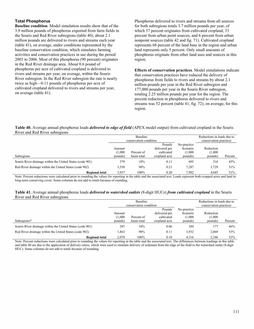
Total Phosphorus Baseline condition. Model simulation results show that of the 3.9 million pounds of phosphorus exported from farm fields in the Souris and Red River subregions (table 40), about 2.1 million pounds are delivered to rivers and streams each year (table 41), on average, under conditions represented by the baseline conservation condition, which simulates farming activities and conservation practices in use during the period 2003 to 2006. Most of this phosphorus (90 percent) originates in the Red River drainage area. About 0.6 pound of phosphorus per acre of cultivated cropland is delivered to rivers and streams per year, on average, within the Souris River subregion. In the Red River subregion the rate is nearly twice as high—0.11 pounds of phosphorus per acre of cultivated cropland delivered to rivers and streams per year, on average (table 41).

Phosphorus delivered to rivers and streams from all sources for both subregions totals 3.7 million pounds per year, of which 57 percent originates from cultivated cropland, 33 percent from urban point sources, and 6 percent from urban nonpoint sources (table 42 and fig. 71). Cultivated cropland represents 68 percent of the land base in the region and urban land represents only 5 percent. Only small amounts of phosphorus originate from other land uses and sources in this region. Effects of conservation practices. Model simulations indicate that conservation practices have reduced the delivery of phosphorus from fields to rivers and streams by about 2.1 million pounds per year in the Red River subregion and 177,000 pounds per year in the Souris River subregion, totaling 2.25 million pounds per year for the region. The percent reduction in phosphorus delivered to rivers and streams was 52 percent (table 41, fig. 72), on average, for this region.

Table 40. Average annual phosphorus loads delivered to edge of field (APEX model output) from cultivated cropland in the Souris River and Red River subregions

Baseline

conservation condition Reductions in loads due to

conservation practices

Subregions

Amount (1,000

pounds) Percent of basin total

Pounds delivered per

cultivated cropland acre

No-practice Scenario

(1,000 pounds)

Reduction (1,000

pounds) Percent

Souris River drainage within the United States (code 901) 379 10% 0.11 695 316 45% Red River drainage within the United States (code 902) 3,558 90% 0.21 7,287 3,729 51%

Regional total 3,937 100% 0.20 7,982 4,045 51% Note: Percent reductions were calculated prior to rounding the values for reporting in the table and the associated text. Loads represent both cropped acres and land in long-term conserving cover. Some columns do not add to totals because of rounding. Table 41. Average annual phosphorus loads delivered to watershed outlets (8-digit HUCs) from cultivated cropland in the Souris River and Red River subregions

Baseline

conservation condition Reductions in loads due to

conservation practices

Subregions*

Amount (1,000

pounds) Percent of basin total

Pounds delivered per

cultivated cropland acre

No-practice Scenario

(1,000 pounds)

Reduction (1,000

pounds) Percent

Souris River drainage within the United States (code 901) 207 10% 0.06 384 177 46% Red River drainage within the United States (code 902) 1,863 90% 0.11 3,932 2,069 53%

Regional total 2,070 100% 0.10 4,316 2,246 52% Note: Percent reductions were calculated prior to rounding the values for reporting in the table and the associated text. The differences between loadings in this table and table 40 are due to the application of delivery ratios, which were used to simulate delivery of sediment from the edge of the field to the watershed outlet (8-digit HUC). Some columns do not add to totals because of rounding.

111

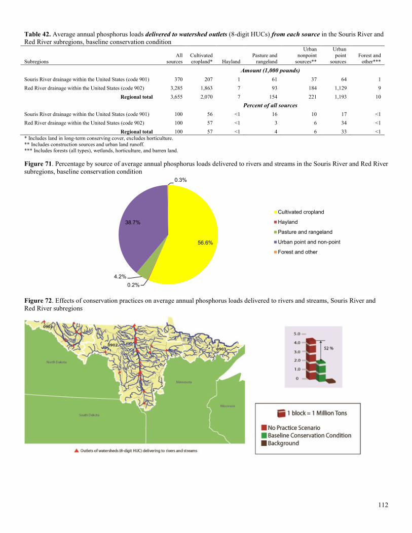
Table 42. Average annual phosphorus loads delivered to watershed outlets (8-digit HUCs) from each source in the Souris River and Red River subregions, baseline conservation condition

Subregions All

sources Cultivated cropland* Hayland

Pasture and rangeland

Urban nonpoint

sources**

Urban point

sources Forest and

other***

Amount (1,000 pounds) Souris River drainage within the United States (code 901) 370 207 1 61 37 64 1 Red River drainage within the United States (code 902) 3,285 1,863 7 93 184 1,129 9

Regional total 3,655 2,070 7 154 221 1,193 10 Percent of all sources Souris River drainage within the United States (code 901) 100 56 <1 16 10 17 <1 Red River drainage within the United States (code 902) 100 57 <1 3 6 34 <1

Regional total 100 57 <1 4 6 33 <1 * Includes land in long-term conserving cover, excludes horticulture. ** Includes construction sources and urban land runoff. *** Includes forests (all types), wetlands, horticulture, and barren land. Figure 71. Percentage by source of average annual phosphorus loads delivered to rivers and streams in the Souris River and Red River subregions, baseline conservation condition

Figure 72. Effects of conservation practices on average annual phosphorus loads delivered to rivers and streams, Souris River and Red River subregions

56.6%

0.2% 4.2%

38.7%

0.3%

Cultivated cropland

Hayland

Pasture and rangeland

Urban point and non-point

Forest and other

112

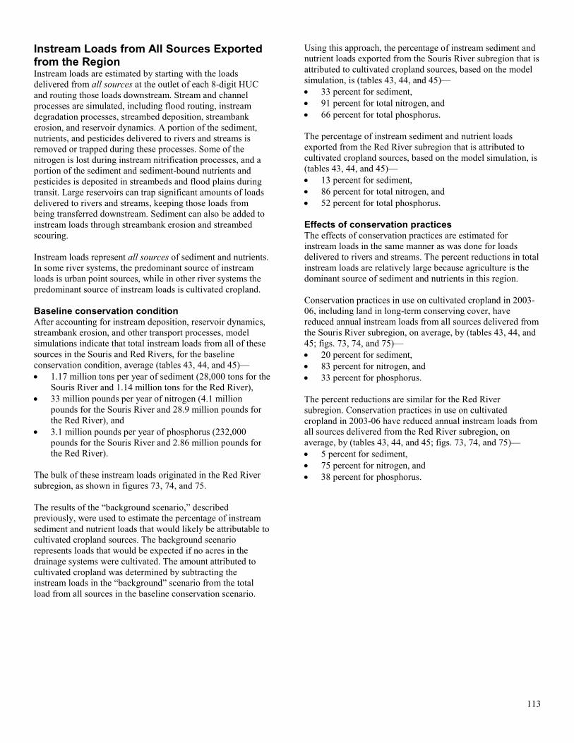
Instream Loads from All Sources Exported from the Region Instream loads are estimated by starting with the loads delivered from all sources at the outlet of each 8-digit HUC and routing those loads downstream. Stream and channel processes are simulated, including flood routing, instream degradation processes, streambed deposition, streambank erosion, and reservoir dynamics. A portion of the sediment, nutrients, and pesticides delivered to rivers and streams is removed or trapped during these processes. Some of the nitrogen is lost during instream nitrification processes, and a portion of the sediment and sediment-bound nutrients and pesticides is deposited in streambeds and flood plains during transit. Large reservoirs can trap significant amounts of loads delivered to rivers and streams, keeping those loads from being transferred downstream. Sediment can also be added to instream loads through streambank erosion and streambed scouring. Instream loads represent all sources of sediment and nutrients. In some river systems, the predominant source of instream loads is urban point sources, while in other river systems the predominant source of instream loads is cultivated cropland. Baseline conservation condition After accounting for instream deposition, reservoir dynamics, streambank erosion, and other transport processes, model simulations indicate that total instream loads from all of these sources in the Souris and Red Rivers, for the baseline conservation condition, average (tables 43, 44, and 45)— • 1.17 million tons per year of sediment (28,000 tons for the

Souris River and 1.14 million tons for the Red River), • 33 million pounds per year of nitrogen (4.1 million

pounds for the Souris River and 28.9 million pounds for the Red River), and

• 3.1 million pounds per year of phosphorus (232,000 pounds for the Souris River and 2.86 million pounds for the Red River).

The bulk of these instream loads originated in the Red River subregion, as shown in figures 73, 74, and 75. The results of the “background scenario,” described previously, were used to estimate the percentage of instream sediment and nutrient loads that would likely be attributable to cultivated cropland sources. The background scenario represents loads that would be expected if no acres in the drainage systems were cultivated. The amount attributed to cultivated cropland was determined by subtracting the instream loads in the “background” scenario from the total load from all sources in the baseline conservation scenario.

Using this approach, the percentage of instream sediment and nutrient loads exported from the Souris River subregion that is attributed to cultivated cropland sources, based on the model simulation, is (tables 43, 44, and 45)— • 33 percent for sediment, • 91 percent for total nitrogen, and • 66 percent for total phosphorus. The percentage of instream sediment and nutrient loads exported from the Red River subregion that is attributed to cultivated cropland sources, based on the model simulation, is (tables 43, 44, and 45)— • 13 percent for sediment, • 86 percent for total nitrogen, and • 52 percent for total phosphorus. Effects of conservation practices The effects of conservation practices are estimated for instream loads in the same manner as was done for loads delivered to rivers and streams. The percent reductions in total instream loads are relatively large because agriculture is the dominant source of sediment and nutrients in this region. Conservation practices in use on cultivated cropland in 2003-06, including land in long-term conserving cover, have reduced annual instream loads from all sources delivered from the Souris River subregion, on average, by (tables 43, 44, and 45; figs. 73, 74, and 75)— • 20 percent for sediment, • 83 percent for nitrogen, and • 33 percent for phosphorus. The percent reductions are similar for the Red River subregion. Conservation practices in use on cultivated cropland in 2003-06 have reduced annual instream loads from all sources delivered from the Red River subregion, on average, by (tables 43, 44, and 45; figs. 73, 74, and 75)— • 5 percent for sediment, • 75 percent for nitrogen, and • 38 percent for phosphorus.

113

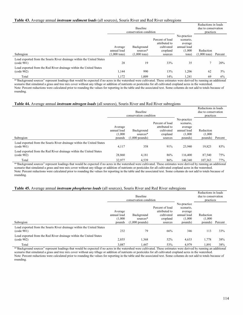
Table 43. Average annual instream sediment loads (all sources), Souris River and Red River subregions

Baseline

conservation condition

Reductions in loads due to conservation

practices

Subregion

Average annual load (1,000 tons)

Background sources*

(1,000 tons)

Percent of load attributed to

cultivated cropland

sources

No-practice scenario, average

annual load (1,000

tons) Reduction

(1,000 tons) Percent Load exported from the Souris River drainage within the United States (code 901) 28 19 33% 35 7 20% Load exported from the Red River drainage within the United States (code 902) 1,144 990 13% 1,206 62 5%

Total 1,172 1,009 14% 1,241 69 6% *“Background sources” represent loadings that would be expected if no acres in the watershed were cultivated. These estimates were derived by running an additional scenario that simulated a grass and tree mix cover without any tillage or addition of nutrients or pesticides for all cultivated cropland acres in the watershed. Note: Percent reductions were calculated prior to rounding the values for reporting in the table and the associated text. Some columns do not add to totals because of rounding. Table 44. Average annual instream nitrogen loads (all sources), Souris River and Red River subregions

Baseline

conservation condition

Reductions in loads due to conservation

practices

Subregion

Average annual load

(1,000 pounds

Background sources*

(1,000 pounds)

Percent of load attributed to

cultivated cropland

sources

No-practice scenario, average

annual load (1,000

pounds)

Reduction (1,000

pounds) Percent Load exported from the Souris River drainage within the United States (code 901) 4,117 358 91% 23,940 19,823 83% Load exported from the Red River drainage within the United States (code 902) 28,860 4,181 86% 116,400 87,540 75%

Total 32,977 4,539 86% 140,340 107,363 77% *“Background sources” represent loadings that would be expected if no acres in the watershed were cultivated. These estimates were derived by running an additional scenario that simulated a grass and tree mix cover without any tillage or addition of nutrients or pesticides for all cultivated cropland acres in the watershed. Note: Percent reductions were calculated prior to rounding the values for reporting in the table and the associated text. Some columns do not add to totals because of rounding. Table 45. Average annual instream phosphorus loads (all sources), Souris River and Red River subregions

Baseline

conservation condition

Reductions in loads due to conservation

practices

Subregion

Average annual load

(1,000 pounds

Background sources*

(1,000 pounds)

Percent of load attributed to

cultivated cropland

sources

No-practice scenario, average

annual load (1,000

pounds)

Reduction (1,000

pounds) Percent Load exported from the Souris River drainage within the United States (code 901) 232 79 66% 346 113 33% Load exported from the Red River drainage within the United States (code 902) 2,855 1,368 52% 4,633 1,778 38%

Total 3,087 1,447 53% 4,979 1,891 38% *“Background sources” represent loadings that would be expected if no acres in the watershed were cultivated. These estimates were derived by running an additional scenario that simulated a grass and tree mix cover without any tillage or addition of nutrients or pesticides for all cultivated cropland acres in the watershed. Note: Percent reductions were calculated prior to rounding the values for reporting in the table and the associated text. Some columns do not add to totals because of rounding.

114

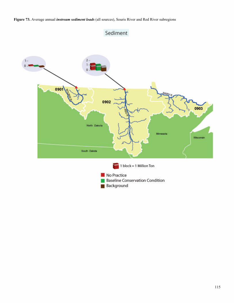
Figure 73. Average annual instream sediment loads (all sources), Souris River and Red River subregions

115

Figure 74. Average annual instream nitrogen loads (all sources), Souris River and Red River subregions

116

Figure 75. Average annual instream phosphorus loads (all sources), Souris River and Red River subregions

117

Chapter 7 Summary of Findings Field Level Assessment Evaluation of practices in use The first Federal conservation efforts on cropland were focused primarily on water management and soil erosion control. Structural practices such as waterways, terraces, and diversions were installed along with appropriate supporting practices. Conservation tillage emerged in the 1970s as a key management practice for enhancing soil quality and further reducing soil erosion. The conservation compliance provisions in the 1985 Farm Bill sharpened the focus to treatment of the most erodible acres—highly erodible land. This legislation created the Conservation Reserve Program as a mechanism for establishing long-term conserving cover on the most erodible cropland through multi-year contracts with landowners. More recently, the focus has shifted from soil conservation and sustainability to a broader goal of reducing all pollution impacts associated with agricultural production. Prominent among new concerns are the environmental effects of nutrient and pesticide export from farm fields. The application of conservation practices in the Souris-Red-Rainy Basin reflects this history of Federal conservation programs and technical assistance. An assessment, based on a farmer survey representing practice use and farming activities for the period 2003–06, found the following: • Structural practices for controlling water erosion are in

use on 18 percent of cropped acres. On the 13 percent of the acres designated as highly erodible land, structural practices designed to control water erosion are in use on 23 percent.

• Structural practices for controlling wind erosion are in use on 20 percent of cropped acres. On the 13 percent of the acres designated as highly erodible land, structural practices designed to control wind erosion are in use on 26 percent.

• Reduced tillage is common in the region; 72 percent of the cropped acres meet criteria for either no-till (17 percent) or mulch till (55 percent). All but 12 percent of the acres had evidence of some kind of reduced tillage on at least one crop.

• About 37 percent of cropped acres are gaining soil organic carbon.

• Producers use either residue and tillage management practices or structural practices, or both, on 89 percent of cropped acres.

• The use of nutrient management practices is more widespread in this region than in other regions. o About 1 percent of cropped acres have no nitrogen

applied. An additional 64 percent of cropped acres meet criteria for timing of nitrogen applications on all crops in the rotation, 78 percent meet criteria for method of application, and 71 percent meet criteria for rate of application (table 10).

o About 2 percent of cropped acres have no phosphorus applied. An additional 79 percent of cropped acres

meet criteria for timing of phosphorus applications on all crops in the rotation, 83 percent meet criteria for method of application, and 55 percent meet criteria for rate of application (table 10).

o Appropriate nitrogen application rates, timing of application, and application method for all crops during every year of production are in use on 38 percent of cropped acres (table 10).

o Good phosphorus management practices (appropriate rate, timing, and method) are in use on 43 percent of the acres on all crops during every year of production (table 10).

o About 25 percent of cropped acres meet nutrient management criteria for both nitrogen and phosphorus management, including acres with no nutrient applications (table 10).

• During the 2003–06 period of data collection, criteria for cover crops were not met on any CEAP sample points in this region.

• The Integrated Pest Management (IPM) indicator showed that about 19 percent of the acres were being managed with a relatively high level of IPM (fig. 11).

• Land in long-term conserving cover, as represented by enrollment in the CRP General Signup, consists of 2.3 million acres in the region, of which 29 percent is highly erodible land.

Annual precipitation over the 47-year simulation averaged about 20 inches for cropped acres in the region. The annual precipitation amount (averaged over all cropped acres) ranged over the 47 years from 12 inches in 1976 to 24 inches in 2005 (fig. 6). Effects of conservation practices Model simulation results show that, for cropped acres in the region, on average conservation practices have— • reduced surface water flow from fields by 7 percent, re-

routing water to subsurface flow pathways (table 13); • reduced wind erosion by 52 percent, from 4.7 tons per

acre without conservation practices to 2.25 tons per acre with conservation practices (table 14);

• reduced sediment loss from fields caused by water erosion by 43 percent, from 0.11 ton per acre without conservation practices to 0.06 ton per acre with conservation practices (table 15);

• reduced total nitrogen loss (volatilization, denitrification, surface runoff, subsurface flow, and windborne losses) from fields by 52 percent, from 49.2 pounds per acre without conservation practices to 23.6 pounds per acre with conservation practices (table 18): o reduced nitrogen lost with windborne sediment by 45

percent, from 21.1 pounds per acre without practices to 11.6 pounds per acre with conservation practices;

o reduced nitrogen lost with surface runoff (attached to sediment and in solution) by 67 percent, from 1.9 pounds per acre without conservation practices to 0.6 pound per acre with conservation practices;

o reduced nitrogen loss in subsurface flows by 71 percent, from 17.3 pounds per acre without

118

conservation practices to 5.0 pounds per acre with conservation practices;

• reduced total phosphorus loss from fields by 57 percent, from 4.7 pounds per acre without conservation practices to 2.0 pounds per acre with conservation practices (table 20); and

• reduced pesticide loss from fields to surface water, resulting in a 78-percent reduction in edge-of-field pesticide risk (all pesticides combined) for aquatic ecosystems and a 74-percent reduction in edge-of-field surface water pesticide risk for humans (table 22).

In this region, conservation practices have a positive effect on soil organic carbon levels for most cropped acres (figs. 26 and 27). Conservation practice use in the region has resulted in an average annual gain in soil organic carbon of 77 pounds per acre per year on cropped acres (table 17). For land in long-term conserving cover (2.3 million acres), soil erosion and sediment loss have been almost completely eliminated. Compared to a cropped condition without conservation practices, total nitrogen loss has been reduced by 77 percent, total phosphorus loss has been reduced by 86 percent, and soil organic carbon has been increased by an average of 274 pounds per acre per year (tables 17, 19, and 20). Conservation treatment needs The adequacy of conservation practices in use in the Souris-Red-Rainy Basin for the period 2003–06 was evaluated to identify conservation treatment needs for five resource concerns (see chapter 5): • Wind erosion. • Sediment loss from fields. • Nitrogen lost with surface runoff (attached to sediment

and in solution). • Nitrogen loss in subsurface flows. • Phosphorus lost to surface water (includes soluble

phosphorus in lateral flow). Not all acres require the same level of conservation treatment. Acres with a high level of inherent vulnerability require more treatment than less vulnerable acres to reduce field-level losses to acceptable levels. Acres with characteristics such as steeper slopes and soil types that promote surface water runoff are more vulnerable to sediment and nutrient losses beyond the edge of the field. Acres that are essentially flat with permeable soil types are more prone to nutrient losses through subsurface flow pathways, most of which return to surface water through drainage ditches, tile drains, natural seeps, and groundwater return flow. Undertreated acres were identified by an imbalance between the level of conservation treatment and the level of inherent vulnerability (matrix approach). Three levels of treatment need were identified: • Acres with a “high” level of need for conservation

treatment consist of the most critical undertreated acres in the region. These are the most vulnerable of the

undertreated acres with the least conservation treatment and have the highest losses of sediment and/or nutrients.

• Acres with a “moderate” level of need for conservation treatment consist of undertreated acres that generally have lower levels of vulnerability and/or have more conservation practice use than acres with a high level of need. The treatment level required is not necessarily less, although it can be, but rather the sediment and nutrient losses are lower and thus there is less potential on a per-acre basis for reducing agricultural pollutant loadings with additional conservation treatment.

• Acres with a “low” level of need for conservation treatment consist of acres that are adequately treated with respect to the level of inherent vulnerability. While gains can be obtained by adding conservation practices to some of these acres, additional conservation treatment would reduce field losses by only a small amount.

Simulation model results (tables 24 through 28) indicate that wind erosion is the principal conservation treatment need in this region. A total of 4.3 million acres need additional treatment for wind erosion, representing 25 percent of cropped acres in the region (fig. 60). All of these acres have a moderate need for additional treatment. These 4.3 million acres have an average wind erosion rate of 4.6 tons per acre per year and lose, on average, 18.8 pounds per acre of nitrogen and 3.2 pounds per acre of phosphorus with windborne sediment each year (table 29). Resource concerns related to water quality were not as pronounced in this region as in other regions of the country, in part because of the lower levels of precipitation, the short growing season, the preponderance of close grown crops in the cropping systems (see table 6), and the widespread use of conservation practices throughout the region. Moreover, acres with a high or moderately high soil runoff or leaching potential represent a small minority of cropped acres in this region (figs. 54 and 56). No acres in the region exceeded the acceptable levels of loss for sediment (2 tons per acre per year), nitrogen in runoff (15 pounds per acre per year), and phosphorus (4 pounds per acre per year) based on the long-term average loss estimates. A small number of acres (about 300,000 acres, representing 2 percent of cropped acres) had average annual losses of nitrogen in subsurface flows above 25 pounds per acre per year, but these were not widespread enough to be detected as a significant conservation treatment need using the matrix approach. The majority of cropped acres in this region—13.2 million acres, representing 75 percent of cropped acres—were determined to have a low level of conservation treatment need. Acres with a low level of need for conservation treatment consist of acres that are adequately treated with respect to the level of inherent vulnerability. In the Souris-Red-Rainy Basin, these 13.2 million acres have an average wind erosion rate of 1.5 tons per acre per year and lose (per acre per year, on average) only 0.05 ton of sediment by water erosion, 1.6 pounds of phosphorus, and 21 pounds of nitrogen (table 29). While gains can be attained by adding conservation practices to some of these acres with a low treatment need, additional

119

conservation treatment would reduce average field losses by only a small amount. Most of the acres that need additional treatment for wind erosion are found in the Red River Basin (code 0902). Twenty-eight percent of the cropped acres in this subregion (4.1 million acres) need additional treatment for wind erosion. Less than 300,000 acres need additional treatment in the Souris River Basin (code 0901) (9 percent of acres in subregion). Loads Delivered to Rivers and Streams within the Region Reductions in field-level losses due to conservation practices, including land in long-term conserving cover, translate into improvements in water quality in streams and rivers in the region. Transport of sediment, nutrients, and pesticides from farm fields to streams and rivers involves a variety of processes and time-lags, and not all of the potential pollutants leaving fields contribute to instream loads. Model simulation results for the Souris and Red Rivers indicate that for the baseline conservation condition, sediment and nutrient loads delivered to rivers and streams from cultivated cropland sources per year, on average, are: • 371,000 tons of sediment (77 percent of loads from all

sources); • 53.3 million pounds of nitrogen (83 percent of loads from

all sources); and • 2.1 million pounds of phosphorus (57 percent of loads

from all sources). Conservation practices in use on cultivated cropland in 2003–06, including land in long-term conserving cover, have reduced sediment and nutrient loads delivered to rivers and streams from cultivated cropland sources per year, on average, by: • 50 percent for sediment; • 75 percent for nitrogen; and • 52 percent for phosphorus. Instream Loads from All Sources Exported from the Region Instream loads are estimated by starting with the loads delivered from all sources at the outlet of each 8-digit HUC and routing those loads downstream. Stream and channel processes are simulated, including flood routing, instream degradation processes, streambed deposition, streambank erosion, and reservoir dynamics. A portion of the sediment, nutrients, and pesticides delivered to rivers and streams is removed or trapped during these processes. Some of the nitrogen is lost during instream nitrification processes, and a portion of the sediment and sediment-bound nutrients is deposited in streambeds and flood plains during transit. Large reservoirs can trap significant amounts of loads delivered to rivers and streams, keeping those loads from being transferred downstream. Sediment can also be added to instream loads through streambank erosion and streambed scouring.

Instream loads represent all sources of sediment and nutrients. After accounting for instream deposition, reservoir dynamics, streambank erosion, and other transport processes, model simulations indicate that total instream loads from all of these sources in the Souris and Red Rivers, for the baseline conservation condition, average (tables 43, 44, and 45)— • 1.17 million tons per year of sediment (28,000 tons for the

Souris River and 1.14 million tons for the Red River), • 33 million pounds per year of nitrogen (4.1 million

pounds for the Souris River and 28.9 million pounds for the Red River), and

• 3.1 million pounds per year of phosphorus (232,000 pounds for the Souris River and 2.86 million pounds for the Red River).

The percentage of instream sediment and nutrient loads exported from the Souris River subregion that is attributed to cultivated cropland sources, based on the model simulation, is (tables 43, 44, and 45)— • 33 percent for sediment, • 91 percent for total nitrogen, and • 66 percent for total phosphorus. The percentage of instream sediment and nutrient loads exported from the Red River subregion that is attributed to cultivated cropland sources, based on the model simulation, is (tables 43, 44, and 45)— • 13 percent for sediment, • 86 percent for total nitrogen, and • 52 percent for total phosphorus. Conservation practices in use on cultivated cropland in 2003-06, including land in long-term conserving cover, have reduced annual instream loads from all sources delivered from the Souris River subregion, on average, by (tables 43, 44, and 45; figs. 73, 74, and 75)— • 20 percent for sediment, • 83 percent for nitrogen, and • 33 percent for phosphorus. The percent reductions are similar for the Red River subregion. Conservation practices in use on cultivated cropland in 2003-06 have reduced annual instream loads from all sources delivered from the Red River subregion, on average, by (tables 43, 44, and 45; figs. 73, 74, and 75)— • 5 percent for sediment, • 75 percent for nitrogen, and • 38 percent for phosphorus.

120

References Arnold, J.G., R. Srinivasan, R.S. Muttiah, and J.R. Williams. 1998. Large area hydrologic modeling and assessment part I: model development.

Journal of the American Water Resources Association. 34(1): 73-89.

Arnold, J.G., R. Srinivasan, R.S. Muttiah, and P.M. Allen. 1999. Continental scale simulation of the hydrologic balance. Journal of the American Water Resources Association. 35(5): 1037-1052.

Arnold, J.G. and N. Fohrer. 2005. SWAT2000: current capabilities and research opportunities in applied watershed modeling. Hydrological Processes. 19(3): 563-572.

Bruulsema, T., Lemunyon, J., and Herz, B. 2009. Know your fertilizer rights. Crops and Soils 42(2), pp 13-16.

Coble, H. 1998. Measuring the Resilience of IPM Systems—The PAMS Diversity Index. Unpublished manuscript. U.S. Department of Agriculture. 1998.

Daly, C., R. P. Neilson, and D. L. Phillips. 1994: A statistical-topographic model for mapping climatological precipitation over mountainous terrain. J. Appl. Meteor., 33, 140–158.

Di Luzio M., G. L. Johnson, C. Daly, Jon K. Eischeid, J.G. Arnold. 2008. Constructing Retrospective Gridded Daily Precipitation and Temperature Datasets for the Conterminous United States. Journal of Applied Meteorology and Climatology. 47(2): 475–497.

Eischeid, Jon K., Phil A. Pasteris; Henry F. Diaz, Marc S. PLantico, and Neal J. Lott. 2000. Creating a serially complete, national daily time series of temperature and precipitation for the western United States.” Journal of Applied Meteorology 39 (September):1580-1591.

Gassman, Philip W., Jimmy R. Williams, Verel W. Benson, R. Cesar Izaurralde, Larry Hauck, C. Allan Jones, Jay D. Atwood, James Kiniry, and Joan D. Flowers. 2005. Historical Development and Applications of the EPIC and APEX Models. Working Paper 05-WP 397, Center for Agricultural and Rural Development, Iowa State University, Ames, IA.

Gassman, P.W., M.R. Reyes, C.H. Green, and J.G. Arnold. 2007. The Soil and Water Assessment Tool: Historical development, applications and future research directions. Transactions of the American Society of Agricultural and Biological Engineers 50(4): 1211-1250.

Gassman, P.W., J.R. Williams, S. Wang, A. Saleh, E. Osei, L. Hauck, C. Izaurralde, and J. Flowers. 2009. The Agricultural Policy Environmental Extender (APEX) model: An emerging tool for landscape and watershed environmental analyses. Technical Report 09-TR 49. CARD, Iowa State Univ., Ames, IA. Available at: http://www.card.iastate.edu/publications/synopsis.aspx?id=1101.

Gassman, P.W., J.R. Williams, S. Wang, A. Saleh, E. Osei, L. Hauck, C. Izaurralde, and J. Flowers. 2010. The Agricultural Policy Environmental

Extender (APEX) model: An emerging tool for landscape and watershed environmental analyses. Trans. of the ASABE. Vol. 53(3): 711-740. Gianessi, L.P., and H.M. Peskin. 1984. An overview of the RFF Environmental Data Inventory--Methods and preliminary results: Resources for the

Future, Washington, D.C., 111 p.

Goebel, J.J., and H.D. Baker. 1987. The 1982 National Resources Inventory Sample Design and Estimation Procedures. Statistical Laboratory, Iowa State University, Ames, IA.

Goebel, J.J. 1998. The National Resources Inventory and its role in U.S. agriculture. In Agricultural Statistics 2000. International Statistical Institute, Voorburg, The Netherlands, 181–192.

Goebel, J.J., and R.L. Kellogg. 2002. Using survey data and modeling to assist the development of agri-environmental policy. In Conference on Agricultural and Environmental Statistical Applications in Rome. National Statistical Institute of Italy, Rome, Italy, 695–705.

Goss, Don W., Robert L. Kellogg, Joaquin Sanabria, Susan Wallace, and Walt Kniesel. 1998. The National Pesticide Loss Database: A Tool for Management of Large Watersheds. Poster presentation at the 53rd annual Soil and Water Conservation Society conference. San Diego, CA, July 5–9., 1998.

Homer, C., J. Dewitz, J. Fry, M. Coan, N. Hossain, C. Larson, N. Herold, A. McKerrow, J.N. VanDriel and J. Wickham. 2007. Completion of the 2001 National Land Cover Database for the Conterminous United States, Photogrammetric Engineering and Remote Sensing, Vol. 73, No. 4, pp 337-341.

Huber, W.C. and R.E. Dickinson. 1988. Storm water management model, version 4: user’s manual.

Izaurralde, R. C., J. R. Williams, W. B. McGill, N. J. Rosenberg, M. C. Quiroga Jakas. 2006. Simulating soil C dynamics with EPIC: Model description and testing against long-term data. Ecol. Model. 192: 362–384.

Kellogg, R.L., M.S. Maizel, and D.W. Goss. 1992. Agricultural Chemical Use and Ground Water Quality: Where Are the Problem Areas? U.S. Department of Agriculture, Soil Conservation Service.

Kellogg, Robert L., Margaret Maizel, and Don W. Goss. 1994. The potential for leaching of agrichemicals used in crop production: A national perspective. Journal of Soil and Water Conservation 49(3):294–298.

Kellogg, Robert L., Don W. Goss, Susan Wallace, and Klaus Alt. 1997. Potential Priority Watersheds for Protection of Water Quality from Non-Point Sources Related to Agriculture. Poster Presentation at the 52nd Annual Soil and Water Conservation Society Conference. Toronto, Ontario, Canada. July 22–25, 1997.

121

Kellogg, Robert L. 2000. Potential Priority Watersheds for Protection of Water Quality from Contamination by Manure Nutrients. Presented at the

Water Environment Federation’s Animal Residuals Management Conference 2000. Kansas City, MO. November 12–14, 2000.

Kellogg, Robert L. Richard F. Nehring, Arthur Grube, Donald W. Goss, and Steven Plotkin. 2002. Environmental indicators of pesticide leaching and runoff from farm fields. In Ball, V. Eldon, and George W. Norton (editors), Agricultural Productivity: Measurement and Sources of Growth. Kluwer Academic Publishers, Boston, MA.

Maresch, W., M.R. Walbridge, and D. Kugler. 2008. Enhancing conservation on agricultural landscapes: A new direction for the Conservation Effects Assessment Project. Journal of Soil and Water Conservation, Nov.-Dec. 2008.

Mausbach, M.J., and A.R. Dedrick. 2004. The length we go: Measuring environmental effects of conservation practices. Journal of Soil and Water Conservation, Sept.-Oct. 2004.

National Agricultural Statistics Service (NASS). 2007. Cropland Data Layer. USDA NRCS Geospatial Data Gateway, http://datagateway.nrcs.usda.gov/

NADP/NTN 2004. National Atmospheric Deposition Program / National Trends Network, http://nadp.sws.uiuc.edu

Nusser, S.M., and J.J. Goebel. 1997. The National Resources Inventory: A long-term multi-resource monitoring programme. Environmental and Ecological Statistics 4:181–204.

Potter, S.R., S. Andrews, J.D. Atwood, R.L. Kellogg, J. Lemunyon, L. Norfleet, and D. Oman. 2006. Model simulation of soil loss, nutrient loss, and change in soil organic carbon associated with crop production. USDA, Natural Resources Conservation Service, Washington, DC. Available at http://www.nrcs.usda.gov/technical/nri/ceap.

Santhi, C., N. Kannan, M. White, M. Di Luzio, J.G. Arnold, X. Wang, and J.R. Williams. 2012. An Integrated Modeling Approach for Estimating the Water Quality Benefits of Conservation Practices at River Basin Scale. J. Environ. Qual. doi:10.2134/jeq2011.0460.

Srinivasan, R.S., J.G. Arnold, and C.A. Jones. 1998. Hydrologic modeling of the United States with the Soil and Water Assessment Tool. International Journal of Water Resources Development. 14(3): 315-325.

U.S. Department of Agriculture. 1989. The Second RCA Appraisal: Analysis of Conditions and Trends. 280 pages.

U.S. Department of Agriculture. 2011. RCA Appraisal 2011: Soil and Water Resources Conservation Act. 100 pages.

U.S. Department of Agriculture, Natural Resources Conservation Service. 2002. 1997 National Resources Inventory Summary Report. Washington, DC. Available at http://www.nrcs.usda.gov/technical/nri.

United States Department of Agriculture, Natural Resources Conservation Service. 2003. Costs Associated With Development and Implementation of Comprehensive Nutrient Management Plans.

United States Department of Agriculture, Natural Resources Conservation Service. 2007. 2003 National Resources Inventory. http://www.nrcs.usda.gov/technical/nri.

United States Department of Agriculture, National Agricultural Statistics Service. 2009. 2007 Census of Agriculture. Database.

USDA-Farm Service Agency. June 2004. Conservation Reserve Program Overview. CRP: Planting for the Future. U.S. Department of Agriculture, Farm Service Agency. Washington, DC.

U.S. Geological Survey. 1980. Hydrologic Unit Map of the United States. U.S. Department of the Interior. Washington, DC.

White, M.J., , C. Santhi, N. Kannan, J. G. Arnold, D. Harmel, L. Norfleet, P. Allen, M. DiLuzio, X. Wang, J. Atwood, E. Haney and M. V. Johnson. 2014. Nutrient delivery from the Mississippi River to the Gulf of Mexico and effects of cropland conservation. J. Soil and Water Conserv. 69(1):26-40.

Wiebe, Keith, and Noel Gollehon, editors. July 2006. Agricultural Resources and Environmental Indicators, 2006 Edition. Chapter 5, Conservation and Environmental Policies—USDA Land Retirement Programs. Economic Information Bulletin Number 16. U.S. Department of Agriculture, Economic Research Service. Washington, DC.

Williams, J. R. 1990. The erosion productivity impact calculator (EPIC) model: A case history. Phil. Trans. R. Soc. Lond. 329: 421-428.

Williams, J. R., C. A. Jones, and P. T. Dyke. 1984. A modeling approach to determining the relationship between erosion and soil productivity. Trans. ASAE 27(1): 129-144.

Williams, J. R., W. L. Harman, M. Magre, U. Kizil, J. A. Lindley, G. Padmanabhan, and E. Wang. 2006. APEX feedlot water quality simulation. Trans. ASAE 49(1): 61-73.

Williams, J. R., R. C. Izaurralde, and E. M. Steglich. 2008. Agricultural Policy/Environmental eXtender Model: Theoretical documentation version 0604. BREC Report # 2008-17. Temple, TX: Texas AgriLIFE Research, Texas A&M University, Blackland Research and Extension Center. Available at: http://epicapex.brc.tamus.edu/downloads/user-manuals.aspx. Accessed 31 January 2010.

122

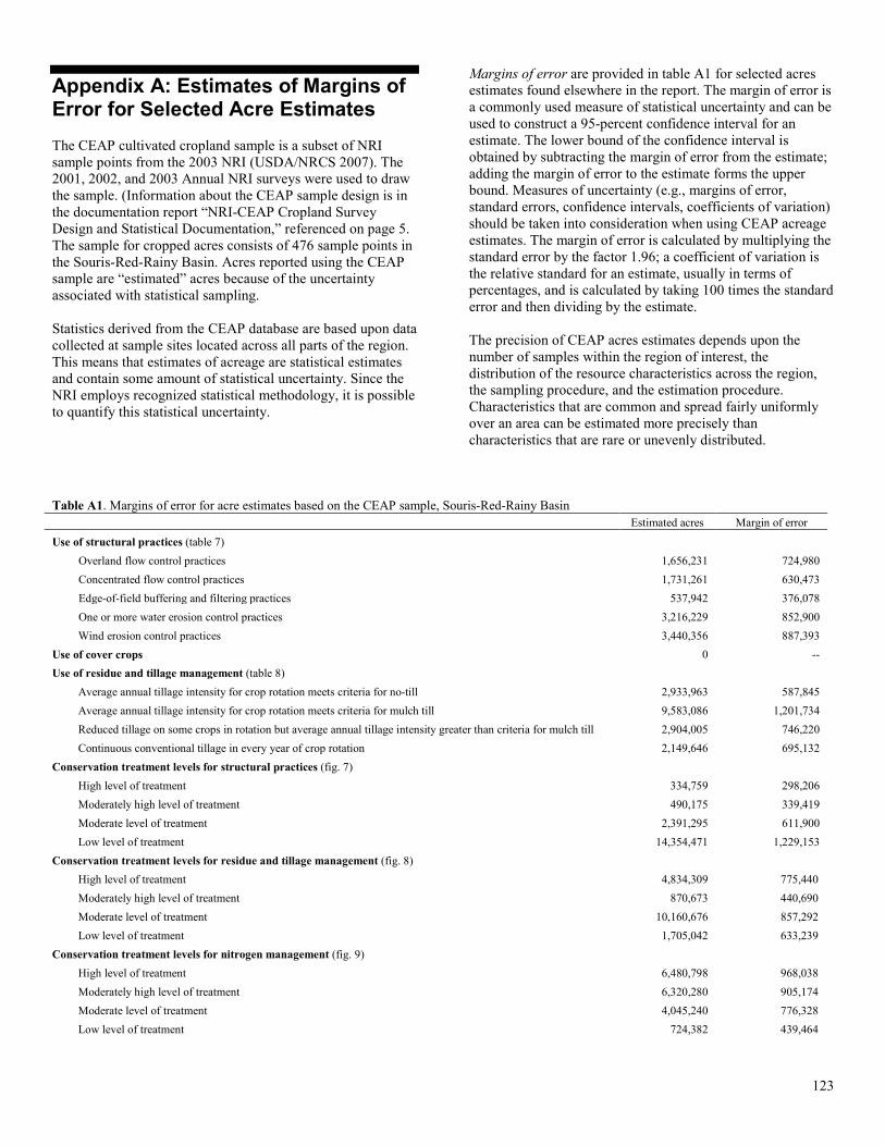
Appendix A: Estimates of Margins of Error for Selected Acre Estimates The CEAP cultivated cropland sample is a subset of NRI sample points from the 2003 NRI (USDA/NRCS 2007). The 2001, 2002, and 2003 Annual NRI surveys were used to draw the sample. (Information about the CEAP sample design is in the documentation report “NRI-CEAP Cropland Survey Design and Statistical Documentation,” referenced on page 5. The sample for cropped acres consists of 476 sample points in the Souris-Red-Rainy Basin. Acres reported using the CEAP sample are “estimated” acres because of the uncertainty associated with statistical sampling. Statistics derived from the CEAP database are based upon data collected at sample sites located across all parts of the region. This means that estimates of acreage are statistical estimates and contain some amount of statistical uncertainty. Since the NRI employs recognized statistical methodology, it is possible to quantify this statistical uncertainty.

Margins of error are provided in table A1 for selected acres estimates found elsewhere in the report. The margin of error is a commonly used measure of statistical uncertainty and can be used to construct a 95-percent confidence interval for an estimate. The lower bound of the confidence interval is obtained by subtracting the margin of error from the estimate; adding the margin of error to the estimate forms the upper bound. Measures of uncertainty (e.g., margins of error, standard errors, confidence intervals, coefficients of variation) should be taken into consideration when using CEAP acreage estimates. The margin of error is calculated by multiplying the standard error by the factor 1.96; a coefficient of variation is the relative standard for an estimate, usually in terms of percentages, and is calculated by taking 100 times the standard error and then dividing by the estimate. The precision of CEAP acres estimates depends upon the number of samples within the region of interest, the distribution of the resource characteristics across the region, the sampling procedure, and the estimation procedure. Characteristics that are common and spread fairly uniformly over an area can be estimated more precisely than characteristics that are rare or unevenly distributed.

Table A1. Margins of error for acre estimates based on the CEAP sample, Souris-Red-Rainy Basin Estimated acres Margin of error

Use of structural practices (table 7) Overland flow control practices 1,656,231 724,980 Concentrated flow control practices 1,731,261 630,473 Edge-of-field buffering and filtering practices 537,942 376,078 One or more water erosion control practices 3,216,229 852,900 Wind erosion control practices 3,440,356 887,393

Use of cover crops 0 -- Use of residue and tillage management (table 8)

Average annual tillage intensity for crop rotation meets criteria for no-till 2,933,963 587,845 Average annual tillage intensity for crop rotation meets criteria for mulch till 9,583,086 1,201,734 Reduced tillage on some crops in rotation but average annual tillage intensity greater than criteria for mulch till 2,904,005 746,220 Continuous conventional tillage in every year of crop rotation 2,149,646 695,132

Conservation treatment levels for structural practices (fig. 7) High level of treatment 334,759 298,206 Moderately high level of treatment 490,175 339,419 Moderate level of treatment 2,391,295 611,900 Low level of treatment 14,354,471 1,229,153

Conservation treatment levels for residue and tillage management (fig. 8) High level of treatment 4,834,309 775,440 Moderately high level of treatment 870,673 440,690 Moderate level of treatment 10,160,676 857,292 Low level of treatment 1,705,042 633,239

Conservation treatment levels for nitrogen management (fig. 9) High level of treatment 6,480,798 968,038 Moderately high level of treatment 6,320,280 905,174 Moderate level of treatment 4,045,240 776,328 Low level of treatment 724,382 439,464

123

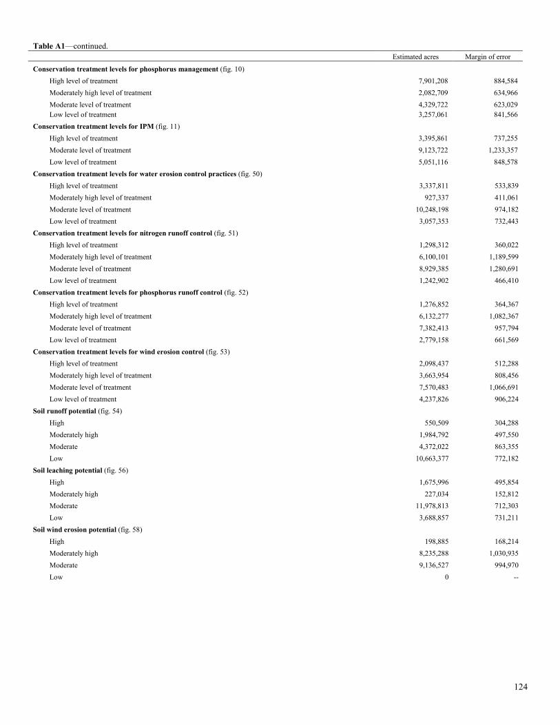
Table A1—continued. Estimated acres Margin of error

Conservation treatment levels for phosphorus management (fig. 10) High level of treatment 7,901,208 884,584 Moderately high level of treatment 2,082,709 634,966 Moderate level of treatment 4,329,722 623,029 Low level of treatment 3,257,061 841,566

Conservation treatment levels for IPM (fig. 11) High level of treatment 3,395,861 737,255 Moderate level of treatment 9,123,722 1,233,357 Low level of treatment 5,051,116 848,578

Conservation treatment levels for water erosion control practices (fig. 50) High level of treatment 3,337,811 533,839 Moderately high level of treatment 927,337 411,061 Moderate level of treatment 10,248,198 974,182 Low level of treatment 3,057,353 732,443

Conservation treatment levels for nitrogen runoff control (fig. 51) High level of treatment 1,298,312 360,022 Moderately high level of treatment 6,100,101 1,189,599 Moderate level of treatment 8,929,385 1,280,691 Low level of treatment 1,242,902 466,410

Conservation treatment levels for phosphorus runoff control (fig. 52) High level of treatment 1,276,852 364,367 Moderately high level of treatment 6,132,277 1,082,367 Moderate level of treatment 7,382,413 957,794 Low level of treatment 2,779,158 661,569

Conservation treatment levels for wind erosion control (fig. 53) High level of treatment 2,098,437 512,288 Moderately high level of treatment 3,663,954 808,456 Moderate level of treatment 7,570,483 1,066,691 Low level of treatment 4,237,826 906,224

Soil runoff potential (fig. 54) High 550,509 304,288 Moderately high 1,984,792 497,550 Moderate 4,372,022 863,355 Low 10,663,377 772,182

Soil leaching potential (fig. 56) High 1,675,996 495,854 Moderately high 227,034 152,812 Moderate 11,978,813 712,303 Low 3,688,857 731,211

Soil wind erosion potential (fig. 58) High 198,885 168,214 Moderately high 8,235,288 1,030,935 Moderate 9,136,527 994,970 Low 0 --

124

Table A1—continued. Estimated acres Margin of error

Level of conservation treatment need for wind erosion Souris-Red-Rainy Basin

High (critical undertreated) 0 -- Moderate (non-critical undertreated) 4,343,365 877,421 Low (adequately treated) 13,227,335 965,508

Souris River drainage within the United States (code 901) High (critical undertreated) 0 -- Moderate (non-critical undertreated) 277,564 233,179 Low (adequately treated) 2,851,836 351,286

Red River drainage within the United States (code 902) High (critical undertreated) 0 -- Moderate (non-critical undertreated) 4,065,801 847,262 Low (adequately treated) 10,375,499 892,157

125

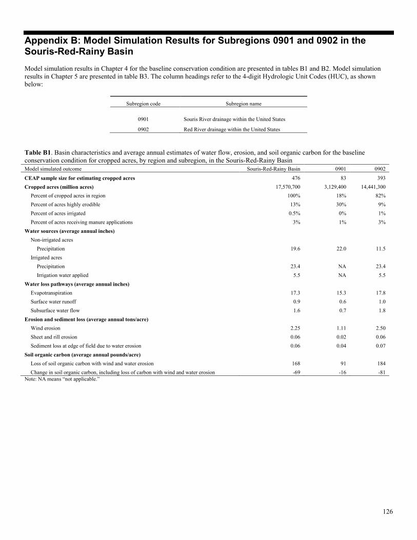
Appendix B: Model Simulation Results for Subregions 0901 and 0902 in the Souris-Red-Rainy Basin Model simulation results in Chapter 4 for the baseline conservation condition are presented in tables B1 and B2. Model simulation results in Chapter 5 are presented in table B3. The column headings refer to the 4-digit Hydrologic Unit Codes (HUC), as shown below:

Subregion code Subregion name

0901 Souris River drainage within the United States

0902 Red River drainage within the United States Table B1. Basin characteristics and average annual estimates of water flow, erosion, and soil organic carbon for the baseline conservation condition for cropped acres, by region and subregion, in the Souris-Red-Rainy Basin Model simulated outcome Souris-Red-Rainy Basin 0901 0902

CEAP sample size for estimating cropped acres 476 83 393 Cropped acres (million acres) 17,570,700 3,129,400 14,441,300

Percent of cropped acres in region 100% 18% 82% Percent of acres highly erodible 13% 30% 9% Percent of acres irrigated 0.5% 0% 1% Percent of acres receiving manure applications 3% 1% 3%

Water sources (average annual inches) Non-irrigated acres

Precipitation 19.6 22.0 11.5 Irrigated acres

Precipitation 23.4 NA 23.4 Irrigation water applied 5.5 NA 5.5

Water loss pathways (average annual inches) Evapotranspiration 17.3 15.3 17.8 Surface water runoff 0.9 0.6 1.0 Subsurface water flow 1.6 0.7 1.8

Erosion and sediment loss (average annual tons/acre) Wind erosion 2.25 1.11 2.50 Sheet and rill erosion 0.06 0.02 0.06 Sediment loss at edge of field due to water erosion 0.06 0.04 0.07

Soil organic carbon (average annual pounds/acre) Loss of soil organic carbon with wind and water erosion 168 91 184 Change in soil organic carbon, including loss of carbon with wind and water erosion -69 -16 -81

Note: NA means “not applicable.”

126

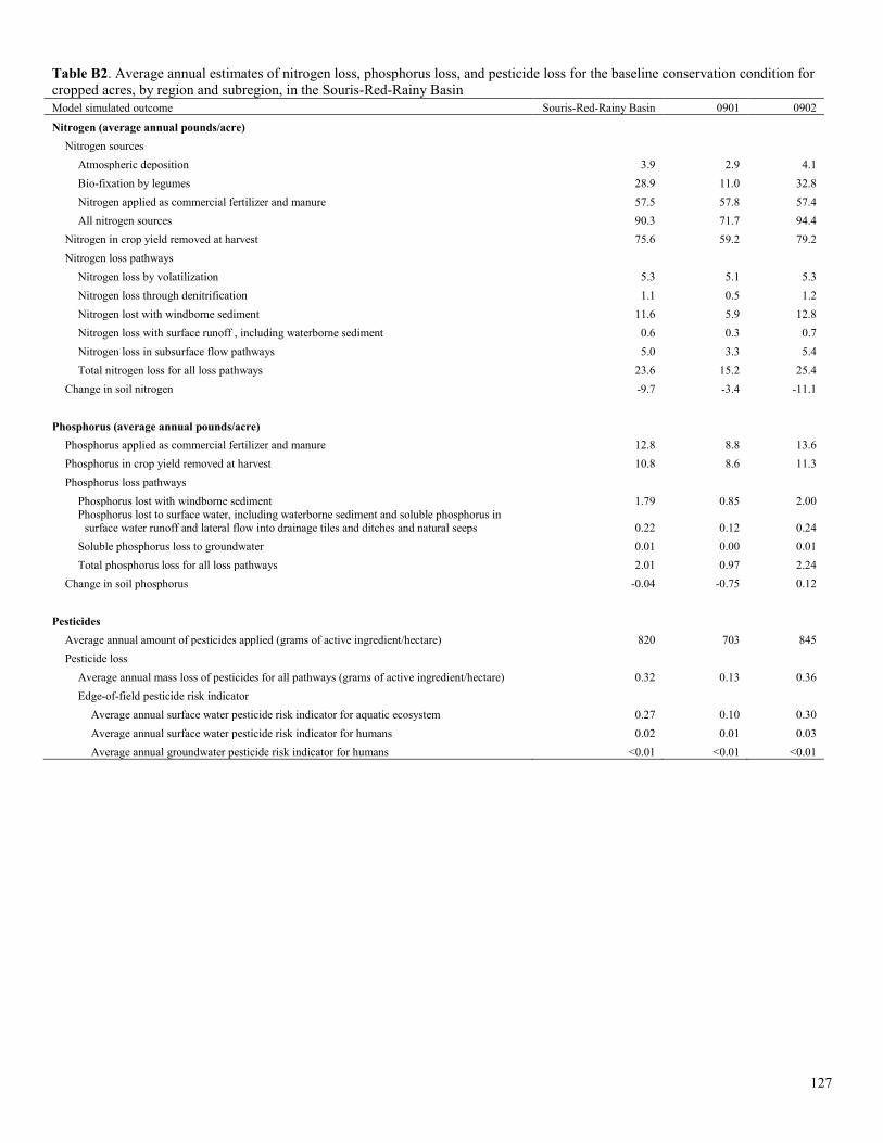
Table B2. Average annual estimates of nitrogen loss, phosphorus loss, and pesticide loss for the baseline conservation condition for cropped acres, by region and subregion, in the Souris-Red-Rainy Basin Model simulated outcome Souris-Red-Rainy Basin 0901 0902

Nitrogen (average annual pounds/acre) Nitrogen sources

Atmospheric deposition 3.9 2.9 4.1 Bio-fixation by legumes 28.9 11.0 32.8 Nitrogen applied as commercial fertilizer and manure 57.5 57.8 57.4 All nitrogen sources 90.3 71.7 94.4

Nitrogen in crop yield removed at harvest 75.6 59.2 79.2 Nitrogen loss pathways

Nitrogen loss by volatilization 5.3 5.1 5.3 Nitrogen loss through denitrification 1.1 0.5 1.2 Nitrogen lost with windborne sediment 11.6 5.9 12.8 Nitrogen loss with surface runoff , including waterborne sediment 0.6 0.3 0.7 Nitrogen loss in subsurface flow pathways 5.0 3.3 5.4 Total nitrogen loss for all loss pathways 23.6 15.2 25.4

Change in soil nitrogen -9.7 -3.4 -11.1 Phosphorus (average annual pounds/acre)

Phosphorus applied as commercial fertilizer and manure 12.8 8.8 13.6 Phosphorus in crop yield removed at harvest 10.8 8.6 11.3 Phosphorus loss pathways

Phosphorus lost with windborne sediment 1.79 0.85 2.00 Phosphorus lost to surface water, including waterborne sediment and soluble phosphorus in

surface water runoff and lateral flow into drainage tiles and ditches and natural seeps 0.22 0.12 0.24 Soluble phosphorus loss to groundwater 0.01 0.00 0.01 Total phosphorus loss for all loss pathways 2.01 0.97 2.24

Change in soil phosphorus -0.04 -0.75 0.12 Pesticides

Average annual amount of pesticides applied (grams of active ingredient/hectare) 820 703 845 Pesticide loss

Average annual mass loss of pesticides for all pathways (grams of active ingredient/hectare) 0.32 0.13 0.36 Edge-of-field pesticide risk indicator

Average annual surface water pesticide risk indicator for aquatic ecosystem 0.27 0.10 0.30 Average annual surface water pesticide risk indicator for humans 0.02 0.01 0.03 Average annual groundwater pesticide risk indicator for humans <0.01 <0.01 <0.01

127

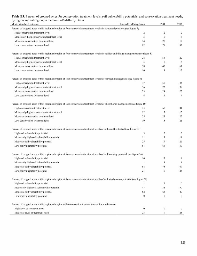
Table B3. Percent of cropped acres for conservation treatment levels, soil vulnerability potentials, and conservation treatment needs, by region and subregion, in the Souris-Red-Rainy Basin Model simulated outcome Souris-Red-Rainy Basin 0901 0902

Percent of cropped acres within region/subregion at four conservation treatment levels for structural practices (see figure 7) High conservation treatment level 2 2 2 Moderately-high conservation treatment level 3 0 3 Moderate conservation treatment level 14 20 12 Low conservation treatment level 82 78 82

Percent of cropped acres within region/subregion at four conservation treatment levels for residue and tillage management (see figure 8)

High conservation treatment level 28 54 22 Moderately-high conservation treatment level 5 0 6 Moderate conservation treatment level 58 45 61 Low conservation treatment level 10 1 12

Percent of cropped acres within region/subregion at four conservation treatment levels for nitrogen management (see figure 9)

High conservation treatment level 37 50 34 Moderately-high conservation treatment level 36 22 39 Moderate conservation treatment level 23 24 23 Low conservation treatment level 4 4 4

Percent of cropped acres within region/subregion at four conservation treatment levels for phosphorus management (see figure 10)

High conservation treatment level 45 65 41 Moderately-high conservation treatment level 12 7 13 Moderate conservation treatment level 25 23 25 Low conservation treatment level 19 5 21

Percent of cropped acres within region/subregion at four conservation treatment levels of soil runoff potential (see figure 54)

High soil vulnerability potential 3 2 3 Moderately high soil vulnerability potential 11 13 11 Moderate soil vulnerability potential 25 19 26 Low soil vulnerability potential 61 66 60

Percent of cropped acres within region/subregion at four conservation treatment levels of soil leaching potential (see figure 56)

High soil vulnerability potential 10 13 9 Moderately high soil vulnerability potential 1 3 1 Moderate soil vulnerability potential 68 75 67 Low soil vulnerability potential 21 9 24

Percent of cropped acres within region/subregion at four conservation treatment levels of soil wind erosion potential (see figure 58)

High soil vulnerability potential 1 5 0 Moderately high soil vulnerability potential 47 31 50 Moderate soil vulnerability potential 52 64 49 Low soil vulnerability potential 0 0 0

Percent of cropped acres within region/subregion with conservation treatment needs for wind erosion High level of treatment need 0 0 0 Moderate level of treatment need 25 9 28

128

END

129