assessment of geometrical features of internal flaws with
TRANSCRIPT
Assessment of Geometrical Features of
Internal Flaws with Artificial Neural
Network Optimized by a Thermodynamic
Equilibrium Algorithm
by
Salman Lari
A thesis
presented to the University of Waterloo
in fulfillment of the
thesis requirement for the degree of
Master of Applied Science
in
Mechanical and Mechatronics Engineering
Waterloo, Ontario, Canada, 2020
©Salman Lari 2020

ii
AUTHOR'S DECLARATION
I hereby declare that I am the sole author of this thesis. This is a true copy of the thesis, including any
required final revisions, as accepted by my examiners.
I understand that my thesis may be made electronically available to the public.

iii
Abstract
In nondestructive testing (NDT), geometrical features of a flaw embedded inside the material such as
its location, length, and orientation angle are critical factors to assess the severity of the flaw and make
post-manufacturing decisions. In this study, a novel evolutionary optimization algorithm has been
developed for machine learning (ML). This algorithm has been inspired by thermodynamic laws and
can be adopted for artificial neural network (ANN). To this end, it was applied to the oscillograms from
virtual ultrasonic NDT to estimate geometrical features of flaws. First, a numerical model of NDT
specimen was constructed using acoustic finite element analysis (FEA) to produce the ultrasonic
signals. The model was validated by comparing the produced signals with the experimental data from
NDT tests on the specimens without and with defects. Then, 750 numerical models containing flaws
with different locations, lengths, and angles were generated by FEA. Next, the oscillograms produced
by the models were divided into 3 datasets: 525 for training, 113 for validation, and 112 for testing.
Training inputs of the network were parameters extracted from ultrasonic signals by fitting them to sine
functions. The proposed evolutionary algorithm was implemented to train the network. Lastly, to
evaluate the network performance, outputs of the network including flaw’s location, length, and angle
were compared with the desired values for all datasets. Deviations of the outputs from desired values
were calculated by a regression analysis. Statistical analysis was also performed by measuring Root
Mean Square Error (RMSE) and Efficiency (E). RMSE in x-location, y-location, length, and angle
estimations are 0.09 mm, 0.19 mm, 0.46 mm, and 0.75, with efficiencies of 0.9229, 0.9466, 0.9140,
and 0.9154, respectively for the testing dataset, which demonstrates high accuracy in estimation.
Results suggest that the proposed AI-based method can be used to characterize flaws with time of flight
NDT approach.
This research introduces optimized smart ultrasonic NDT as an exact and rapid method in
detection of internal flaw, its geometrical features, and also proves the need to replace this method with
conventional method which requires interpretation of the human.

iv
Acknowledgements
First and foremost, I would like to express my sincere appreciation to my supervisor Prof. Hyock-Ju
Kwon for his inspirations and guidance throughout my MASc study. His tolerance as a supervisor and
never-ending energy for bringing novel technical ideas should be highly appreciated. So truly THANK
YOU for everything.
My sincere thanks also go to my colleagues and friends Moslem SadeghiGoughari, Yanjun Qian,
Jeong-Woo Han for their support and assistance during my studies at the University of Waterloo.
Finally, I would like to express my deepest gratitude to my parents for their love, prayers, caring and
continuing support for educating and preparing me for my future. My appreciation likewise extends to
my sister for her true love and support throughout my life.

v
Dedication
To my beloved parents.
vi
Table of Contents
AUTHOR'S DECLARATION ............................................................................................................... ii
Abstract ................................................................................................................................................. iii
Acknowledgements ............................................................................................................................... iv
Dedication .............................................................................................................................................. v
List of Figures ....................................................................................................................................... ix
List of Tables ........................................................................................................................................ xi
Chapter 1 Introduction ........................................................................................................................... 1
1.1 Non-Destructive Testing .............................................................................................................. 1
1.1.1 Applications .......................................................................................................................... 1
1.1.2 Methods ................................................................................................................................. 1
1.1.2.1 Acoustic Emission (AE)................................................................................................. 2
1.1.2.2 Visual Testing (VT) ....................................................................................................... 2
1.1.2.3 Radiography Testing (RT) ............................................................................................. 2
1.1.2.4 Magnetized Testing (MT) .............................................................................................. 3
1.1.2.5 Ultrasonic Testing (UT) ................................................................................................. 3
1.1.2.6 Liquid Penetrant Testing (PT) ........................................................................................ 3
1.1.2.7 Electromagnetic Testing (ET) ........................................................................................ 3
1.1.2.8 Leak Testing (LT) .......................................................................................................... 4
1.1.2.9 Infrared Testing (IRT) .................................................................................................... 4
1.1.2.10 Magnetic Flux Leakage (MFL) .................................................................................... 4
1.1.2.11 Comparison of Methods ............................................................................................... 5
1.2 Ultrasonic Testing (UT) ............................................................................................................... 7
1.2.1 Components of Ultrasonic Test System ................................................................................ 8
1.2.1.1 Pulser-Receiver Unit ...................................................................................................... 8
1.2.1.2 Ultrasonic Transducers .................................................................................................. 8
1.2.2 Arrangement of Transducers ................................................................................................. 9
1.2.3 Display Test Data ................................................................................................................ 10
1.2.3.1 A-Scan .......................................................................................................................... 10
1.2.3.2 B-Scan .......................................................................................................................... 11
1.2.3.3 C-Scan .......................................................................................................................... 12
1.2.4 Analysis of Ultrasonic Data ................................................................................................ 12

vii
1.2.5 Applications ......................................................................................................................... 13
1.2.6 Advantages and Disadvantages ........................................................................................... 13
1.3 Project Goals .............................................................................................................................. 13
1.4 Review of Thesis Chapters ......................................................................................................... 14
Chapter 2 NDT, Research History ........................................................................................................ 15
2.1 Introduction ................................................................................................................................ 15
2.2 Quantitative Non-Destructive Testing (QNDE) ......................................................................... 15
2.3 Smart Ultrasonic NDT ................................................................................................................ 17
2.4 NDT Acoustic Modeling ............................................................................................................ 20
2.5 Evolutionary Optimization Algorithms ...................................................................................... 22
Chapter 3 Numerical Simulation and NDT Device .............................................................................. 23
3.1 Introduction ................................................................................................................................ 23
3.2 Acoustic Modeling ..................................................................................................................... 24
3.3 Finite Element Analysis (FEA) .................................................................................................. 24
3.4 Experimental Validation ............................................................................................................. 26
3.5 Extracting Acoustic Parameters ................................................................................................. 28
3.6 Artificial Intelligence (AI) .......................................................................................................... 28
3.6.1 Artificial Neural Network (ANN) ....................................................................................... 29
3.6.2 ANN-Based Prediction ........................................................................................................ 32
Chapter 4 Thermodynamic Equilibrium Algorithm ............................................................................. 34
4.1 Evolutionary Algorithm.............................................................................................................. 34
4.2 Thermodynamics ........................................................................................................................ 34
4.3 Thermodynamic Equilibrium Algorithm .................................................................................... 34
4.3.1 Initialize the Thermodynamic Systems ............................................................................... 36
4.3.2 Thermodynamic Systems Coupling..................................................................................... 36
4.3.3 Compute Equilibrium Temperature and Volume ................................................................ 37
4.3.4 Update System Thermodynamic State ................................................................................ 39
4.3.5 Check for Entropy Increase ................................................................................................. 40
4.3.6 Check for Thermodynamic Equilibrium .............................................................................. 41
Chapter 5 Modeling, ANN, and Algorithm Results ............................................................................. 42
5.1 Introduction ................................................................................................................................ 42
5.2 Validation of Acoustic FEA ....................................................................................................... 42

viii
5.3 Optimization Results .................................................................................................................. 44
5.4 ANN Training ............................................................................................................................ 49
5.5 ANN Testing .............................................................................................................................. 51
5.6 Discussion .................................................................................................................................. 54
5.7 Suggestions for Future Research................................................................................................ 55
Bibliography ........................................................................................................................................ 56

ix
List of Figures
Figure 1-1 Example of ultrasonic test for jet engine turbine blade root test. ......................................... 7
Figure 1-2 Components of ultrasonic test system. ................................................................................. 9
Figure 1-3 Pitch-Catch method. ........................................................................................................... 10
Figure 1-4 An example of A-scan. ....................................................................................................... 11
Figure 1-5 A two-dimensional B-scan. ................................................................................................ 12
Figure 2-1 Automatic testing of the mock-ups [28]. ............................................................................ 16
Figure 2-2 Processed images at different configurations. (a) 16 elements at 0.25, (b) 16 elements at
0.125, (c) 32 elements at 0.25, (d) 32 elements at 0.125, (e) 64 elements at 0.25 and (f) 64 elements at
0.125 [30]. ............................................................................................................................................ 17
Figure 2-3 The general processing flow of computerized ultrasonic imaging inspection [45]. ........... 19
Figure 2-4 Ultrasound signal representation [42] . ................................................................................ 19
Figure 2-5 Schematic process of Schmidt rebound hammer test [46]. ................................................. 20
Figure 2-6 Simulation model of crack-free cylinder [53]. .................................................................... 22
Figure 3-1 Flowchart of numerical method to estimate crack features. ............................................... 23
Figure 3-2 (a) Schematic of NDT specimen; (b) meshed FEA model. ................................................ 25
Figure 3-3 Drawings of prepared specimens: (a) with a circular hole; (b) with a vertical slit (all
dimensions are in mm). ........................................................................................................................ 27
Figure 3-4 Experiment setup for ultrasonic NDT test. ......................................................................... 28
Figure 3-5 The three main components of an AI system. .................................................................... 29
Figure 3-6 An example of a real neuron [63]. ...................................................................................... 30
Figure 3-7 Simplified mathematical model of real nerve [63]. ............................................................ 30
Figure 3-8 Three-layer perceptron with full connections [63]. ............................................................ 31
Figure 3-9 Topology of the implemented neural network .................................................................... 33
Figure 4-1 Flowchart of optimization thermodynamic equilibrium algorithm..................................... 35
Figure 4-2 Initial thermodynamic state of the coupled systems. .......................................................... 37
Figure 4-3 Equilibrium thermodynamic state of the coupled systems. ................................................ 39
Figure 5-1 Comparison of ultrasonic signals from acoustic FEA and NDT experiments for the samples:
(a) without defect, (b) with 4-mm circular hole in the middle, and (c) with 10-mm vertical slit in the
bottom edge. ......................................................................................................................................... 43
Figure 5-2 3D plot of function f1 (Ackley’s function). ......................................................................... 44

x
Figure 5-3 (a) Initial systems, (b) systems at iteration 17, (c) systems at iteration 34, and (d) systems at
final iteration. ....................................................................................................................................... 46
Figure 5-4 Minimum costs of TEA, GA, and PSO versus iteration are compared in problem 𝑓1
(convergence speed). ............................................................................................................................ 47
Figure 5-5 Ultrasonic responses to the variations of location, length, and angle of the embedded crack
produced by acoustic FEA models....................................................................................................... 50
Figure 5-6 Boxplots of normalized acoustic inputs for the neural network. ........................................ 51
Figure 5-7 Comparison of geometrical parameters of the flaws calculated by the FFNNTEA model with
the desired values; (a) crack x location, (b) crack y location, (c) crack length, (d) crack angle. ......... 52
Figure 5-8 Regression analysis performed over the crack location, length, and angle estimations
calculated by ANN model. ................................................................................................................... 53

xi
List of Tables
Table 1-1 Different methods of NDT and their comparison. ................................................................. 5
Table 3-1 Geometrical parameters of a crack in the FEA model. ........................................................ 26
Table 5-1 Performance of numerical simulation. ................................................................................. 44
Table 5-2 Details of the functions. ....................................................................................................... 47
Table 5-3 Linear regression between ANN outputs and desired values. .............................................. 54
Table 5-4 Performance of ANN model in geometry estimations of an embedded crack. .................... 54

1
Chapter 1
Introduction
1.1 Non-Destructive Testing
Non-destructive Testing (NDT) is an examination technique to evaluate the integrity of a material, a
mechanical component or other parts without causing physical damage [1]. NDT is the use of special
equipment and methods to learn something about an object without harming the object. The term
nondestructive testing usually implies that a nonliving object, such as a piece of metal, is being
evaluated. NDT methods are used to make sure that important parts on airplanes and automobiles and
in nuclear power plants are free of defects that could lead to an accident. NDT is also used in many
other industries to make sure that parts do not have defects that would make the customer unhappy.
The inspection and measurement methods used in the field of NDT are largely based on the scientific
principles of physics and chemistry [2]. Non-destructive testing refers to a set of methods for assessing
and determining the properties of devices and components that do not cause any damage or change in
the system [3].
1.1.1 Applications
Non-destructive testing is widely used in many industries. Among them, the following can be
mentioned [4]:
• Power industry
• Automobile manufacturing
o Engine parts
o Body
• Civil engineering
o Structure
o Foundation
o Water transmission networks
o Roads and road construction
• Oil and gas industry
o Oil and gas pipes
• Aviation
1.1.2 Methods
In this section, the most common methods used in non-destructive tests are introduced.

2
1.1.2.1 Acoustic Emission (AE)
When a solid is under stress, the defects in it cause high-frequency sound waves. These waves are
propagated in matter and can be received by special sensors, and by analyzing these waves, the type of
fault, its location, and its intensity can be determined. Acoustic emission is a new method in the field
of non-destructive testing. This method can be used to identify and locate various defects in load-
bearing structures and their components. Rapid discharge of energy from a concentrated source inside
the body causes transient elastic waves and their propagation in matter. This phenomenon is called
acoustics emission. Depending on the propagation of the waves from the source to the surface of the
material, they can be recorded by sensors and thus obtain information about the existence and location
of the source of the propagation of the waves. These waves can have frequencies up to a few MHz.
Ultrasonic sensors in the range of 20 kHz to 1 MHz are used to hear the sound of materials and structural
failure, and the common frequencies in this method are in the range of 150-300 kHz. Depending on the
type of application, the devices used can be in the form of a small porTable device or a large device of
tens of channels. A single sensor, along with related tools for acquiring and measuring emission
acoustic signals, forms an acoustic emission channel. The multi-channel system is used for purposes
such as locating resources or testing areas that are too large for a single sensor. The components
available on all devices for signal reception are: sensor, preamplifier, filter and amplifier [5].
1.1.2.2 Visual Testing (VT)
This method is the most basic and simplest method of testing quality control and equipment monitoring.
In this way, the quality controller must visually check the items. Of course, cameras are sometimes
used to send images to a computer and the computer detects faults. The sorting method, which is
especially used to control the quality of screws, is an example of a visual control method by a computer
[6].
1.1.2.3 Radiography Testing (RT)
A radiography testing is using gamma and X-rays, which can penetrate many materials to examine
materials and detect product defects. In this method, X-rays or radioactive radiation are directed to the
part and are reflected on the film after passing through the part. Thickness and interior features make
the spots appear darker or lighter in the film [7].

3
1.1.2.4 Magnetized Testing (MT)
In this method, iron particles are poured on a material with a magnetic property and a magnetic field is
induced in it. If there is scratches or cracks on the surface or near the surface, magnetic poles will form
at the fault site or the magnetic field in that area will be distorted. These magnetic poles absorb iron
particles. As a result, faults can be detected by the iron particles aggregation [8].
1.1.2.5 Ultrasonic Testing (UT)
In this method, high-frequency, low-amplitude ultrasonic waves are sent into the part. These waves are
reflected back after each collision, and some of these waves go to the sensor and the sensor receives it.
From the amplitude and time of return of these waves, the characteristics of this rupture can be
understood. Applications of this method include measuring thickness and detecting defects in parts [9].
1.1.2.6 Liquid Penetrant Testing (PT)
In this method, the surface of the part is covered with a visible colored liquid or fluorescent. After a
while, this liquid penetrates into the cracks and surface cavities of the piece. The liquid is then removed
from the surface of the object and the emitter is sprayed on the surface. The difference in the brightness
of the penetrating liquid and the emitter makes it easy to see surface defects.
This test is used to detect defects that have a way to the surface and can be used on most materials
of any type, while the roughness of the test surface must be appropriate. In this method, we must first
clean the surface from grease and contamination, then spray the penetrating liquid on the surface and
wait for at least five minutes for the penetrating liquid to penetrate into the defect, then clean the surface
and spray the emitter on the surface. The material is usually white. If there is a defect on the surface,
its effect on the surface is clear [10].
1.1.2.7 Electromagnetic Testing (ET)
In this method, an electric Eddy current is induced using a variable magnetic field in a conductive
material, and this electric current is measured. The presence of faults such as cracks in the material
causes interruptions in this flow, and thus the presence of such a defect can be realized. In addition,
different materials have different permeability electrical conductivity, so some materials can be
classified by this method [11].

4
1.1.2.8 Leak Testing (LT)
Various methods are used to detect leaks in pressure vessels and so on, the most important of which
are: electric earphones, pressure gauges, gas or penetrating barriers, halogen diodes, mass spectrometry,
as well as soap bubble testing [12].
1.1.2.9 Infrared Testing (IRT)
One of these methods is to monitor the condition and predict the defects of mechanical and electrical
machines using thermal analysis because the performance of each device is always accompanied by
heat dissipation and usually any mechanical and electrical defects in the equipment occur with
increasing or decreasing temperature. The heat released from the outer surface of objects is released in
the form of infrared radiation that is not visible to the human eye. But this radiation can be seen through
thermographic cameras, which are the most advanced and complete equipment in the field of thermal
analysis.
Thermal analyses can be used to identify and detect faults such as improper electrical connections,
loose parts and equipment, metallurgical changes, overload, improper cooling, improper voltage,
improper connection and conduction, dirty equipment, environmental pollution, oxidation of
connections, poor capacity, corrosion and external erosion, lack of overlap and excessive vibrations,
and many other defects that ultimately cause defects in parts and equipment [13].
1.1.2.10 Magnetic Flux Leakage (MFL)
Magnetic imaging of metal surfaces by magnetic field sensors is a widely used technique in non-
destructive surface testing to detect defects in metal specimens. Among magnetic imaging techniques,
magnetic flux leak test is a widely used method in non-destructive testing of ferromagnetic metal
surfaces such as transmission pipes and oil and gas storage tanks. In this method, the ferromagnetic
sample is magnetized by a permanent magnet or a coil near the saturation zone. The presence of any
discontinuities in the material, such as cracks, causes a localized leakage of flux at the crack site. The
distribution and severity of leakage fluxes provide useful information about the location and dimensions
of the crack. This leakage flux can be measured by a magnetic sensor. The properties of the magnetic
sensor are very effective on the ability of the test system to detect cracks and corrosion with different
dimensions [14].

5
1.1.2.11 Comparison of Methods
Table 1-1 Different methods of NDT and their comparison.
Method Applications Disadvantages and limitations
Liquid penetrant
• Non-porous materials
• Weld inspection, soldering, casting
materials, forging materials,
aluminum parts, discs and turbine
blades, rotary
• Requires access to the tested
surface
• Defects must be broken at the
surface.
• The surface may need to be
cleaned
• Crack-like defects that are
very narrow, especially when
exposed to a force that causes
them to close, as well as very
shallow defects, are difficult to
detect.
• Depth of defect cannot be
measured.
Magnetized
• Materials with magnetic properties
• Surface defects and near-surface
defects can be detected by this
method.
• Can be used for welding, pipes, rods,
castings, forging materials, extruded
materials, engine parts, axles and
gears
• Fault detection is affected by
factors such as field strength
and direction.
• Requires a clean and relatively
smooth surface
• Need to hold the clamp for the
field generator
• The test piece must be non-
magnetic before the test,
which is difficult for some
parts and materials to do.
• The depth of the defects
cannot be measured.
Ultrasonic
• Metallic and non-metallic materials
and composites
• Surface and non-surface defects
• Can be used for welds, fittings, rods,
castings, forging materials, engine
and aircraft parts, building
components, concrete, as well as
widely for detecting defects in
pressurized tanks and oil and gas
transmission pipes.
• Also to determine the thickness and
properties of the material
• To monitor burnout
• It is generally by contact,
sometimes directly and
sometimes through the
interface
• Requires different sensors for
different applications;
generally in terms of
frequency range
• Sensitivity is a function of the
frequency used, and some
materials, due to their
structure, cause the ultrasonic
waves to propagate
significantly. Return waves
from such waves are

6
generally difficult to
distinguish from noise.
• This method is difficult to
apply to very thin parts.
Neutron
radiography
• Metallic and non-metallic materials
and composites
• Pyrotechnics, resins, plastics,
honeycomb structures, radioactive
materials, high-density materials and
materials containing hydrogen
• The test piece must be placed
between the radiation
emitting source and the
receiver.
• The size of the radiation
generator reactor is very
large.
• It is difficult to place test
components in parallel.
• Radiation hazards
• Cracks should be placed
parallel to the rays to be
recognizable.
• Sensitivity reduction by
increasing the thickness of
the piece
X-ray radiography
• Metallic and non-metallic materials
and composites
• Used for all shapes and forms;
casting, welding, electronics,
aerospace, marine and automobile
industries
• Both sides of the piece must
be accessed.
• Test results are largely
dependent on determining the
focal length, voltage, and
exposure time of the
radiation.
• Radiation hazards
• Cracks should be placed
parallel to the rays to be
recognizable.
• Sensitivity reduction by
increasing the thickness of
the piece
Gamma radiography
• It is generally used for thick and
dense materials.
• Used for all shapes and forms;
casting, welding, electronics,
aerospace, marine and automobile
industries
• It is usually used in a place where x-
rays cannot be used due to its high
thickness.
• Both sides of the piece must
be accessed.
• The sensitivity of this method
is not as high as x-rays.
• Radiation hazards
• Cracks should be placed
parallel to the rays to be
recognizable.
• Sensitivity reduction by
increasing the thickness of
the piece
Electromagnetic • Metals, alloys and conductors of
electricity
• For materials sorting
• Requires different sensors for
different applications
7
• Surface and near surface defects can
be detected by this method.
• Can be used for pipes, wires,
bearings, tracks, non-metallic
electrotyping, aircraft parts, discs
and turbine blades, car axle
• Although the sensors in this
method are non-contact, the
sensor must be located very
close to the piece.
• Low penetration (usually
about 5 mm)
Magnetic flux
leakage
• Metals, alloys and magnetic
materials
• Diagnosis of micrometer cracks
• Surface and deep defects can be
detected by this method.
• Can be used for pipes, tanks, wires,
bearings, tracks, non-metallic
electrotyping, aircraft parts, discs
and turbine blades, car axle
• Can be used in magnetic
materials
1.2 Ultrasonic Testing (UT)
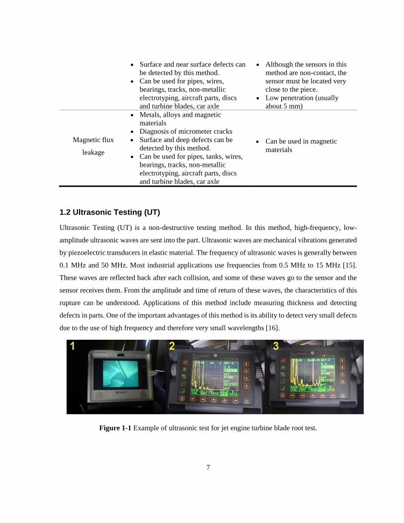
Ultrasonic Testing (UT) is a non-destructive testing method. In this method, high-frequency, low-
amplitude ultrasonic waves are sent into the part. Ultrasonic waves are mechanical vibrations generated
by piezoelectric transducers in elastic material. The frequency of ultrasonic waves is generally between
0.1 MHz and 50 MHz. Most industrial applications use frequencies from 0.5 MHz to 15 MHz [15].
These waves are reflected back after each collision, and some of these waves go to the sensor and the
sensor receives them. From the amplitude and time of return of these waves, the characteristics of this
rupture can be understood. Applications of this method include measuring thickness and detecting
defects in parts. One of the important advantages of this method is its ability to detect very small defects
due to the use of high frequency and therefore very small wavelengths [16].
Figure 1-1 Example of ultrasonic test for jet engine turbine blade root test.

8
1.2.1 Components of Ultrasonic Test System
The components of the ultrasonic test system are shown in Figure 1-2. In this system, the pulser sends
an electric wave to the transmitter transducer. These very short waves (usually about 0.1µs) are
repetitive (about 1 ms) and have a range of hundreds of volts. The transducer converts this electric wave
into sound. The sound wave propagates inside the material and is reflected in the presence of any
discontinuity in the material. The wave reflected by the transducer is received by the receiver and
converted into an electric wave. These waves are then displayed on an oscilloscope and may also be
sent to a computer for more detailed analysis [17].
1.2.1.1 Pulser-Receiver Unit
The Pulser-Receiver is used in field applications and workshops and usually has an oscilloscope for
displays. The main task of this unit is to send the stimulus signal to the transmitter transducer and
receive the signal from the receiver transducer. The unit also usually has multiple microprocessors for
calibration and data analysis purposes [18].
1.2.1.2 Ultrasonic Transducers
The transducers used in the ultrasound test are made of piezoelectric crystals. There are several types
of these transducers, each with its own characteristics. The most important of these features that
distinguish them are [19]:
• Convergent: transducers that have a concave shape and wave rays are concentrated in the
center.
• Flat: the surface of these transducers is flat.
• Receiver-Transmitter: transducers that are used as both receivers and transmitters.
• Longitudinal: transducers that send or receive longitudinal ultrasonic waves.
• Shear: transducers that send or receive ultrasonic shear waves.
• Phased array: in fact, these transducers consist of a number of transducers, each of which can
be stimulated separately.

9
Figure 1-2 Components of ultrasonic test system.
1.2.2 Arrangement of Transducers
In the ultrasonic test, the arrangement of the transducers is as follows:
1. Pulse-Echo: in this method, a transducer is used both as a transmitter and as a receiver. The
transducer sends a pulse into the sample, and the signal is reflected in the presence of a defect,
and part of the reflected signal is received again by the transducer.
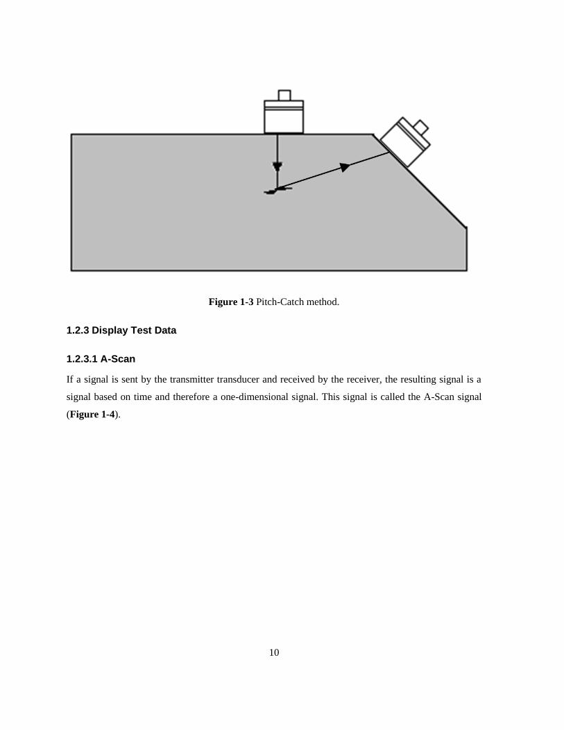
2. Pitch-Catch: in this method, the transmitter transducer sends a signal and the receiver
transducer receives it (Figure 1-3).
3. Through transmission: it is similar to the pitch-catch method, except that the transducer is
placed on the other side of the sample and receives a signal that has passed through the sample
and not reflected inside it.
10
Figure 1-3 Pitch-Catch method.
1.2.3 Display Test Data
1.2.3.1 A-Scan
If a signal is sent by the transmitter transducer and received by the receiver, the resulting signal is a
signal based on time and therefore a one-dimensional signal. This signal is called the A-Scan signal
(Figure 1-4).

11
Figure 1-4 An example of A-scan.
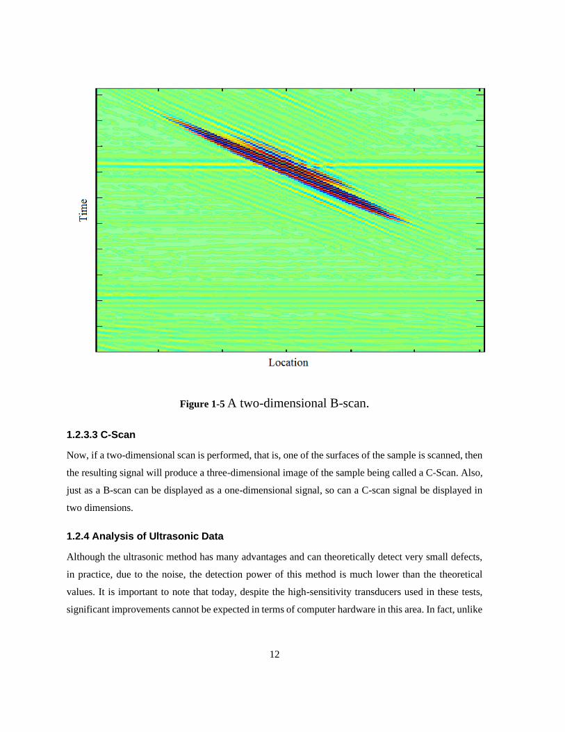
1.2.3.2 B-Scan
If we move the transducer over the test sample and a signal is sent and received at any point, a set of
one-dimensional signals will result. The resulting signal is a two-dimensional matrix that can be
represented as a two-dimensional image. This type of display is called a B-Scan ultrasonic signal.
Sometimes the non-scan signal is displayed as a one-dimensional signal, so that each scan is determined
when the signal has a maximum amplitude, so for each position of the transducer we will have some
time and this amount of time can be plotted by location (Figure 1-5).
12
Figure 1-5 A two-dimensional B-scan.
1.2.3.3 C-Scan
Now, if a two-dimensional scan is performed, that is, one of the surfaces of the sample is scanned, then
the resulting signal will produce a three-dimensional image of the sample being called a C-Scan. Also,
just as a B-scan can be displayed as a one-dimensional signal, so can a C-scan signal be displayed in
two dimensions.
1.2.4 Analysis of Ultrasonic Data
Although the ultrasonic method has many advantages and can theoretically detect very small defects,
in practice, due to the noise, the detection power of this method is much lower than the theoretical
values. It is important to note that today, despite the high-sensitivity transducers used in these tests,
significant improvements cannot be expected in terms of computer hardware in this area. In fact, unlike

13
many other tests in this method, the restriction is not on hardware but on the methods used in processing
ultrasonic signals [20].
1.2.5 Applications
• Metallic and non-metallic materials and composites
• Surface and non-surface defects
• Can be used for welds, fittings, rods, castings, forging materials, engine and aircraft parts,
building components, concrete, as well as widely for detecting defects in pressure vessels and
oil and gas transmission pipes
• Also to determine the thickness and properties of the material
• To monitor burnout
1.2.6 Advantages and Disadvantages
Advantages:
• High penetration power, which can detect defects in the depth of matter.
• Distinguish very small defects such as cracks: Due to the high frequency and therefore the low
wavelength of the waves used in this method, defects with very small dimensions can be
detected. As a rule of thumb, in the theory of size, the smallest defect that can be detected in
this way is equal to half the wavelength used.
• High accuracy in determining the location and size of defects
Disadvantages:
• It is generally using contact, sometimes directly and sometimes through the interface
• Requires different sensors for different applications; generally in terms of frequency range
• Functional sensitivity is a function of the frequency used, and some materials, due to their
structure, cause the ultrasonic waves to propagate significantly. Return waves from such
materials are generally difficult to distinguish from noise.
• This method is difficult to apply to very thin parts.
• The manual operation of the ultrasonic device requires high user skill.
• Data interpretation requires high technical knowledge.
• This method is difficult to apply to irregular, rough, very small, thin, and heterogeneous
surfaces.
1.3 Project Goals
The present project is an attempt to intelligently diagnose component flaws using ultrasonic NDT by
an acoustic modeling and optimization, which can be used to improve the level of the diagnostic process
in industrial use. At present, many models of flaw diagnosis have been performed with the help of
NDT. In some models, attempts have been made to increase the accuracy and speed of defect detection
by using effective parameters in flaw diagnosis and using intelligent methods.
14
In this project, the goal is to try to determine the relationship between specimen ultrasonic signal and
flaw diagnosis by examining the acoustic parameters in flawless specimen and comparing it with the
conditions of having defect within the part. In the modeling section, using the finite element method,
the process of acoustic propagation is simulated in specimen and by extracting the signal profile of the
specimen, the sample is examined to diagnose the presence or absence of flaw. In the next step, the
NDT process is intelligentized and the detection process is performed using acoustic signal.
An ultrasonic NDT device has been implemented to conduct accurate and optimized examinations
of the flaw detection process. An artificial intelligent system has been used to estimate the geometrical
characteristics of the defect. The final achievements of this project include the following:
1. Provide an acoustic model to simulate the ultrasonic NDT process
2. Quantitative diagnosis of crack location
3. Assessment of geometrical features of crack using artificial neural network
4. Optimizing the neural network for high performance
1.4 Review of Thesis Chapters
In the second chapter, an overview of the existing research in the field of NDT will be given and its
modeling. There is also a brief overview of AI methods.
The numerical method of modeling with finite element analysis, implementation of NDT setup, and
crack geometrical features estimation using an artificial neural network is examined in Chapter 3.
In chapter 4, a new evolutionary algorithm is introduced which called the Thermodynamic
Equilibrium Algorithm for optimal neural network in NDT process.
Chapter 5 also includes the results of the constructed model and the capability of NDT method in
detection of the crack geometrical features inside the specimen.

15
Chapter 2
NDT, Research History
2.1 Introduction
Ultrasonic testing is recognized as one of the most common and important methods for a range of
applications in non-destructive testing (NDT) [21]. In this method, ultrasonic energy is propagated into
the tested solids as the form of high-frequency and low-amplitude ultrasound waves. Ultrasound waves
are excited by the mechanical vibration generated by piezoelectric transducers in elastic matter. The
popular frequencies of ultrasound waves in applications are generally between 0.1 MHz and 50 MHz,
and in most industrial NDT, the frequency ranges from 0.5 MHz to 5 MHz [22]. These waves are then
reflected by the back surface or internal discontinuities of the material, and a part of the reflected waves
are received by the same or a different piezoelectric transducer and converted to electrical signals,
called A-scan signals. Characteristics of this discontinuity can be discerned from the amplitude and
timing of the A-scan signals [23]. Applications of this method include thickness measurement and
defect detection in the components [24]. One of the important advantages of ultrasonic NDT is its
ability to detect small defects due to the use of high frequency, and hence short wavelength [25].
However, in most of the applications, it aims to detect only whether cracks and/or defects exist or not
[21].
2.2 Quantitative Non-Destructive Testing (QNDE)
Quantitative non-destructive evaluation (QNDE) is a branch of NDT techniques to estimate sizes,
shapes and locations of flaws, and eventually to assess the health state of a material or a structure [26].
QNDE encompasses a broad range of disciplines including quantitative measurement techniques,
physical models for computational analysis, statistical considerations, quantitative designs of
measurement systems, specifications for flaw detection and characterization, system validation and
performance reliability. Achenbach [26] provided extensive reviews of QNDE and related ultrasonic
techniques including laser-based ultrasonics and acoustic microscopy for crack detection and for the
determination of elastic constants.
Chatillon et al [27] proposed a numerical model for ultrasonic non-destructive testing of components
of complex geometry in the nuclear industry. They proposed a new concept of phase array contact
transducer.

16
Chassignole et al [28] utilized NDT in austenitic stainless steel welds of the primary coolant piping
system for the nuclear industry. They described the characteristics of the mock-ups inspected. Two
side-drilled holes with a diameter of 2 mm were machined in the mock-ups (Figure 2-1).
Figure 2-1 Automatic testing of the mock-ups [28].
Le Jeune et al. [29] proposed a plane wave imaging method for ultrasonic NDT. This method was
applied to multimodal imaging of solids in immersion.
Sutcliffe et al. [30] applied real-time full matrix capture (FMC) for ultrasonic NDT with acceleration
of post-processing through graphic hardware. Full matrix capture allows for the complete ultrasonic
time domain signals for each transmit and receive element of a linear array probe to be retrieved. They
suggested several optimization approaches to speed up the FMC inspection process with particular
emphasis on data parallelization over the graphic process unit (GPU) and provided experimental results
based on real-world scenarios where FMC can be used as a real-time inspection process. They
quantified their results obtained from each of the experimental tests (Figure 2-2).

17
Figure 2-2 Processed images at different configurations. (a) 16 elements at 0.25, (b) 16 elements at
0.125, (c) 32 elements at 0.25, (d) 32 elements at 0.125, (e) 64 elements at 0.25 and (f) 64 elements at
0.125 [30].
S To this end, flaw characterization based on ultrasonic NDT has been largely studied by analytical
[31], experimental [32] and numerical [33] methods to classify them based on their location, size, and
orientation. In recent years, with the dramatic advancement of computing power, the interest in the use
of AI approach to solve NDE problems has been rapidly growing, particularly in the interpretation of
NDT signals for detection and characterization of flaws.
2.3 Smart Ultrasonic NDT
Some well-known AI approaches have been implemented in many researches on ultrasonic NDT. For
the feature extraction from raw data, conventional signal processing methods have been widely

18
adopted, such as discrete Fourier transform (DFT) [34], discrete wavelet transform (DWT) [35],
principal component analysis (PCA) [36] or the genetic algorithm (GA) [37]. For the classification of
features, a variety of machine learning techniques have been used, including singular value
decomposition (SVD) [38], support vector machines (SVM) [39], and sparse coding (SC) [40]. Neural
network (NN)-based learning systems have also been employed, including artificial neural network
(ANN) [41], convolutional neural network (CNN) [42], and deep learning (DL) [43] for damage
characterization.
For example, Sambath et al. [44] adopted a signal processing technique based on DWT for feature
extraction and applied ANN to classify defects in ultrasonic NDT. However, their algorithm could only
categorize the defects into four types: porosity, lack of fusion, and inclusion and non-defect; no
geometrical information of the defects could be obtained. The DWT analyses the signal by
decomposing it into its coarse and detailed information which is accomplished with the use of
successive high-pass and low-pass filtering and subsampling operations, on the basis of the following
equations:
𝑦ℎ𝑖𝑔ℎ(𝑘) = ∑ 𝑥(𝑛). 𝑔(2𝑘 − 𝑛)
𝑛
(2-1)
𝑦𝑙𝑜𝑤(𝑘) = ∑ 𝑥(𝑛). ℎ(2𝑘 − 𝑛)
𝑛
(2-2)
where 𝑦ℎ𝑖𝑔ℎ(𝑘) and 𝑦𝑙𝑜𝑤(𝑘) are the outputs of high-pass and low-pass filters with impulse response
𝑔 and ℎ, respectively, after sub sampling by two (decimation).
Ye et al. [45] compared the performance of CNN-based DL with conventional computer vision
approaches and concluded that DL outperformed all conventional approaches. They presented a
diagram describing the sequential process from ultrasonic signal capture to automatic result generation
(Figure 2-3). However, their DL system could only tell whether a defect exists, and was not able to
report further information, such as location and size.

19
Figure 2-3 The general processing flow of computerized ultrasonic imaging inspection [45].
Meng et al. [42] used a deep CNN to classify the defects in carbon fiber reinforced polymer (CFRP)
(Figure 2-3). However, their framework could identify only the depths of delamination defects using
A-scan signals. The shape of the defect could be obtained from C-scan signals, i.e. by combining
multiple A-scan signals at different locations.
Figure 2-4 Ultrasound signal representation [42] .
Toghroli et al. [46] evaluated the parameters affecting the results of structural health monitoring
using adaptive neuro fuzzy inference system (ANFIS), where the fuzzy logic was combined with the
neural network to obtain a new network architecture. They applied this method to examine how the

20
material properties affect the readings of Schmidt rebound hammer. Figure 2.4 depicts the schematic
process of Schmidt rebound hammer test.
Figure 2-5 Schematic process of Schmidt rebound hammer test [46].
Munir et al. [47] used deep neural network (DNN) with drop out regularization to classify defects in
weldments and showed that proposed DNN architecture could classify defects with high accuracy
without extracting any feature from ultrasonic signals. However, their DNN could detect only the
existence of the flaws without further geometrical information of the flaws. They compared the testing
performance of single hidden layer feed forward neural network on single frequency database and
mixed frequencies database of ultrasonic signals.
2.4 NDT Acoustic Modeling
Although there have been abundant studies applying AI to flaw characterization, most of them can just
discern whether defects exist or not, or types of defects, not capable of predicting more detailed
geometrical features. This may be partly attributed to the lack of real NDT data for various features of

21
the flaws. Note that all AI-based methods are data driven approaches where their ability and
performance are highly dependent on the quantity and quality of training dataset. Unfortunately, there
are very limited number of experimental or real engineering data with detailed information on the flaws,
which highly limits the employment of data-driven approaches for NDT. One way to circumvent the
scarcity of experimental NDT data is to produce the data through realistic numerical simulation. Two
classical analytical scattering models have been used to simulate the interaction of ultrasonic waves
with flaws: the Kirchhoff approximation (KA) [48] and Geometrical Theory of Diffraction (GTD) [49].
Recently there have been other analytical approaches based on Physical Theory of Diffraction (PTD)
[50, 51] accounting for wave reflection and diffraction. However, these analytical approaches are not
easy to implement for numerical simulation. Instead, the numerical acoustic modeling with finite
element analysis (FEA) enables the prediction of the propagation of acoustic fields [51] under various
conditions in both frequency domain and the time domain. There are several studies that have employed
acoustic FEA to simulate the ultrasonic QNDE of the components containing various flaws.
For example, Zou et al. [52] used acoustic FEA to simulate the ultrasonic NDT of hollow components
using phased array transducers. They introduced a new array pattern, which is different in structure
from the commonly used arrays, such as linear array, annular array, 2-D-plannar array, or etc. The
governing equation derived from the momentum equation (Euler's equation) and continuity equation
is:
1
𝜌0𝑐𝑠2
𝜕2𝑝
𝜕𝑡2+ ∇. (−
1
𝜌(∇𝑝 − 𝑞𝑑)) = 𝑄𝑚 (2-3)
where 𝑝 is the total acoustic pressure, 𝜌0 is the fluid density, 𝑐𝑠 is the speed of sound, 𝑄𝑚 is the
monopole source, 𝑞𝑑 is the dipole source, 𝑡 is the time variable and ∇ is the divergence operator.
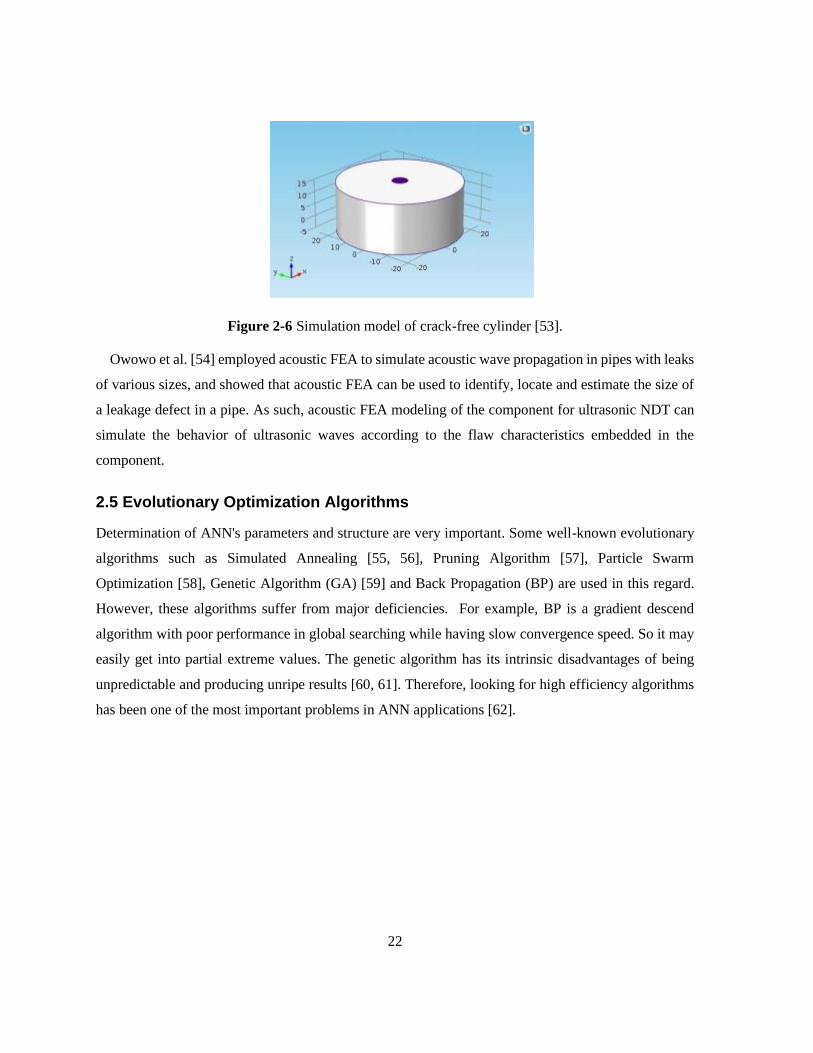
The reliability of the NDT is the basis of NDT technology, and it is the focus of technical research
by many scholars. Tian et al. [53] investigated the detection reliability of ultrasonic NDT with acoustic
FEA using COMSOL and explored the variation of the ultrasonic detection amplitude with the angle
between the sound beam and the crack. Their numerical simulation verification model of ultrasonic
testing was a crack-free cylinder with a diameter of 50 mm and a height of 20 mm (Figure 2-6).
22
Figure 2-6 Simulation model of crack-free cylinder [53].
Owowo et al. [54] employed acoustic FEA to simulate acoustic wave propagation in pipes with leaks
of various sizes, and showed that acoustic FEA can be used to identify, locate and estimate the size of
a leakage defect in a pipe. As such, acoustic FEA modeling of the component for ultrasonic NDT can
simulate the behavior of ultrasonic waves according to the flaw characteristics embedded in the
component.
2.5 Evolutionary Optimization Algorithms
Determination of ANN's parameters and structure are very important. Some well-known evolutionary
algorithms such as Simulated Annealing [55, 56], Pruning Algorithm [57], Particle Swarm
Optimization [58], Genetic Algorithm (GA) [59] and Back Propagation (BP) are used in this regard.
However, these algorithms suffer from major deficiencies. For example, BP is a gradient descend
algorithm with poor performance in global searching while having slow convergence speed. So it may
easily get into partial extreme values. The genetic algorithm has its intrinsic disadvantages of being
unpredictable and producing unripe results [60, 61]. Therefore, looking for high efficiency algorithms
has been one of the most important problems in ANN applications [62].

23
Chapter 3
Numerical Simulation and NDT Device
3.1 Introduction
NDT of industrial part can provide useful information to operators during manufacturing . Today, with
the advancement of ultrasonic NDT technologies, the use of this method as a diagnostic and localization
tool for growing cracks is necessary. This chapter simulates the process of industrial ultrasonic NDT to
locate a flaw. This location can help operators in the follow-up procedures and decisions. In the first
part of the modeling, the finite element method is used to solve the problem of acoustic pressure in the
specimen and the received signal of the specimen is analyzed to check for the presence of the crack and
its location. In order to estimate the geometrical characteristics of the crack from the specimen surface
signal profile, a reverse method using a neural network is used. Figure 3-1 shows the flowchart for the
numerical method used to estimate the geometrical features of the crack.
Figure 3-1 Flowchart of numerical method to estimate crack features.

24
3.2 Acoustic Modeling
The pressure acoustics simulation requires primarily the time-dependent (transient) equation for
acoustics modeling. The acoustic wave equation can be written in scalar form as:
1
𝜌𝑐2
𝜕2𝑝𝑡
𝜕𝑡2 + ∇. (−1
𝜌(∇𝑝𝑡 − 𝑞𝑑)) = 𝑄𝑚 (3-1)
where 𝑝𝑡 is the total acoustic pressure, 𝜌 is the matter density, c is the speed of sound, 𝑞𝑑 is the dipole
domain source, and 𝑄𝑚 is the monopole domain source. In the wave equation, the speed of sound and
density are in general space-dependent and only slowly vary in time, i.e., at a much slower temporal
scale than the variations of acoustic amplitudes.
Boundary conditions at walls are defined with a hard boundary equation, in which the normal
component of the acceleration (and also the velocity) is zero:
−𝑛 ∙ (−1
𝜌(∇𝑝𝑡 − 𝑞𝑑)) = 0 (3-2)
In case of a constant matter density 𝜌 in the medium with no dipole domain source (𝑞𝑑 = 0) at the
boundary, Equation (3-2) implies that the normal derivative of the pressure is zero:
𝜕𝑝𝑡
𝜕𝑛= 0 (3-3)
Sound hard boundaries are valid for both transient and intransient cases to mimic the effect of
impedance mismatch between metal and air. This boundary condition is mathematically identical to the
symmetry condition.
Pressure equation in Equation (3-2) defines the boundary condition that acts as a pressure source at
the boundary, which means that an acoustic pressure constant 𝑝0 is specified and maintained at the
boundary: 𝑝𝑡 = 𝑝0. In the frequency domain, 𝑝0 is the amplitude of a harmonic pressure source.
3.3 Finite Element Analysis (FEA)
The problem was numerically modeled and analyzed using COMSOL Multiphysics software (Release
5.4) for FEA. The NDT specimen made of aluminum was modeled as a 2D square of 100 mm × 100
mm. The top-left corner of the square was chamfered at 45 angle to apply pressure source boundary.
A line crack was modelled inside the specimen (Figure 3-2).

25
Figure 3-2 (a) Schematic of NDT specimen; (b) meshed FEA model.
As the training procedure of an ANN needs a huge amount of data for an accepTable performance,
cracks with different geometrical features were modeled by the numerical simulation. For crack
characterization, four geometrical parameters of a crack were defined and varied as listed in Table 3-
1, while ultrasound waves were emitted by a line source at A and the reflected waves were received at
B in Figure 3-2 (a).
(a)
(b)

26
Table 3-1 Geometrical parameters of a crack in the FEA model.
Parameter Candidates
Crack x location, x (mm) 10, 30, 50, 70, 90
Crack y location, y (mm) 10, 30, 50, 70, 90
Crack length, l (mm) 3, 5, 8, 10, 13
Crack Angle, 𝜃 (°) 0, 30, 60, 90, 120, 150
In order to avoid acoustic wave transition through the sides which are confined by the air, the walls
of the specimen and the crack surface were defined as sound hard boundaries. As indicated in Figure
3-2 (b), the input pulse was applied on the surface of the 45° chamfered corner. The amplitude and
frequency of the pulse were 1 Pa and 0.5 MHz, respectively. The reflected waves were evaluated with
the pressure responses collected on the top right surface of the specimen as shown in Figure 3-2 (b).
Triangular elements were used for FEA modeling as shown in Figure 3-2 (b), as it is well suited to
irregular meshing. For a 10 mm long crack located horizontally in the center of the specimen, the total
number of elements and average mesh quality were 25987 and 0.9899 respectively, with mesh size
ranging from 0.002 mm to 1 mm. Mesh independency was checked and the maximum error of 3.9%
was achieved. For the simulation, acoustic parameters for aluminum were selected from the software
library.
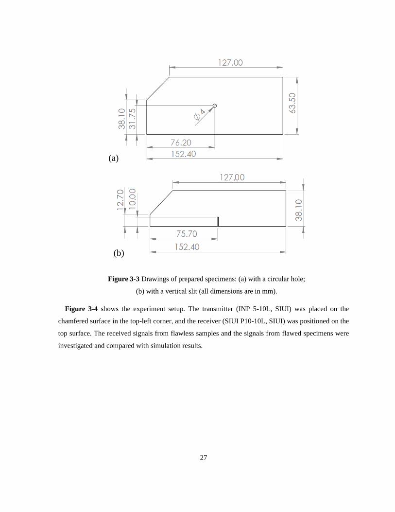
3.4 Experimental Validation
Experiments were conducted to validate the FEA modelling. Two aluminum specimens were machined
to have rectangular shapes with their top left corner chamfered at 45°. The dimensions of the first
specimen was 152.4 mm (L) x 63.3 mm (H) x 63.3 mm (t) (6 in x 2.5 in x 2.5 in) with 25.4 mm (1 in)
chamfer length, and the second one was 152.4 mm (L) x 38.1 mm (H) x 38.1 mm (t) (6 in x 1.5 in x 1.5
in) with the same chamfer length. Ultrasonic NDTs were performed on both specimens following the
schematic shown in Figure 3-2 (a). Two sets of tests were conducted on each sample. The one was on
the fresh-made specimen without defect, and the other was performed after an artificial defect was
created. In the first specimen, a circular hole of 4 mm diameter was drilled in the middle (Figure 3-3
(a)). As for the second specimen, a vertical slit with 10 mm length and 1 mm width was created in the
middle of bottom surface (Figure 3-3 (b)).
27
Figure 3-4 shows the experiment setup. The transmitter (INP 5-10L, SIUI) was placed on the
chamfered surface in the top-left corner, and the receiver (SIUI P10-10L, SIUI) was positioned on the
top surface. The received signals from flawless samples and the signals from flawed specimens were
investigated and compared with simulation results.
(a)
(b)
Figure 3-3 Drawings of prepared specimens: (a) with a circular hole;
(b) with a vertical slit (all dimensions are in mm).

28
Figure 3-4 Experiment setup for ultrasonic NDT test.
3.5 Extracting Acoustic Parameters
In the pulse-echo ultrasound system, the transmitter probe emits an ultrasonic pulse in a short duration.
Although excited at the center frequency, the probe gives out pulse with a range of frequency, called
bandwidth. A series of sine waves may be extracted within the bandwidth. As a result, the received
signals are also a combination of sine waves. In this paper, eight sine wave functions were used to
approximate the response. The response from the receiver probe can thus be recognized as the
summation of the sine functions as shown in Equation (3-4).
𝑓 = ∑ 𝑎𝑖 sin(𝑏𝑖𝑥 + 𝑐𝑖)
8
𝑖=1
(3-4)
In Equation (3-4), amplitude 𝑎𝑖, frequency 𝑏𝑖, and phase angle 𝑐𝑖 were considered as features derived
from the response. Therefore, in total 24 parameters could be derived from each ultrasonic signal. These
parameters were found with curve fitting to the ultrasonic signal using "Trust-Region" algorithm.
3.6 Artificial Intelligence (AI)
The main purpose of artificial intelligence is to develop patterns or algorithms that machines need to
perform cognitive activities. Activities that humans can do well. An artificial intelligence system should
be able to do the following:
1. Knowledge storage
2. Using the stored knowledge to solve the problem
3. Gain new knowledge through experimentation
4. Replacing new knowledge if it is useful and dominating existing knowledge
29
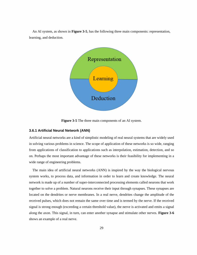
An AI system, as shown in Figure 3-5, has the following three main components: representation,
learning, and deduction.
Figure 3-5 The three main components of an AI system.
3.6.1 Artificial Neural Network (ANN)
Artificial neural networks are a kind of simplistic modeling of real neural systems that are widely used
in solving various problems in science. The scope of application of these networks is so wide, ranging
from applications of classification to applications such as interpolation, estimation, detection, and so
on. Perhaps the most important advantage of these networks is their feasibility for implementing in a
wide range of engineering problems.
The main idea of artificial neural networks (ANN) is inspired by the way the biological nervous
system works, to process data, and information in order to learn and create knowledge. The neural
network is made up of a number of super-interconnected processing elements called neurons that work
together to solve a problem. Natural neurons receive their input through synapses. These synapses are
located on the dendrites or nerve membranes. In a real nerve, dendrites change the amplitude of the
received pulses, which does not remain the same over time and is termed by the nerve. If the received
signal is strong enough (exceeding a certain threshold value), the nerve is activated and emits a signal
along the axon. This signal, in turn, can enter another synapse and stimulate other nerves. Figure 3-6
shows an example of a real nerve.
Deduction

30
Figure 3-6 An example of a real neuron [63].
An artificial neuron is in fact a computational model inspired by real human neurons. At a glance, a
nerve model should include inputs that act as synapses. These inputs are multiplied by weights to
determine the signal strength. Finally, a math operator decides whether or not to activate the neuron,
and if the answer is yes, determines the output. Therefore, the artificial neural network processes
information using a simplified model of the real nerve. Figure 3-7 suggests a simple model for
describing a neuron (a node in an artificial neural network).
Figure 3-7 Simplified mathematical model of real nerve [63].

31
Although the method of modeling the neuron is an essential part of the key points in the efficiency
of the neural network, the way in which the connections and structure of the neural network are
established is also a very important and influential factor. It should be noted that the topology of the
human brain is so complex that it cannot be used as a model for applying the structure of the neural
network, because the brain arrangement uses many elements and according to the existing artificial
intelligence knowledge, this is not possible.
One of the simplest yet most efficient layouts to use in neural network building models is the multi
layer perceptron (MLP). It consists of one input layer, one or more hidden layers and one output layer.
In this structure, all the neurons in one layer are connected to all the neurons in the next layer. This
layout is a so-called network with full connections. Figure 3-8 shows a three-layer perceptron network.
It is noteworthy that the number of neurons in each layer is independent of the number of other neurons
in the layers.
Figure 3-8 Three-layer perceptron with full connections [63].
Given that the neural network is a simplified model of the body's nerves, it can be learned just like
them. In other words, the neural network is able to learn the process in patterns using the information
it receives from the input. Therefore, similar to humans, the process of learning in the neural network
has been inspired by human models, so that many examples should be provided to the network many
times so that it can follow the desired output by changing the weights (w) of the network. In other

32
words, the goal of training a neural network is to find the right weights and biases in order to minimize
the error.
3.6.2 ANN-Based Prediction
Artificial neural networks (ANNs) are connected nodes and links representing neurons between inputs
and outputs. The knowledge of the problem is reflected by the values of weights and biases assigned to
each link and node. When fed with input data, the ANN can generate output according to its knowledge.
To obtain useful output, the neural network must be trained with realistic data to adjust the weights and
biases.
The most common neural network architecture is three-layer feed-forward neural network (FFNN).
As inferred by its name, a FFNN propagates the signal from input to output unidirectionally, and can
approximate nonlinear continuous functions [63]. In training, the signal path is reversed and back-
propagation (BP) algorithm is used to train the FFNN. In back-propagation training, the algorithm is
looking for an optimal set of the network weights and biases to minimize the error between the
prediction and desired output. The commonly employed error function is based on mean squared error
(MSE) in Equation 3-5:
𝑀𝑆𝐸 =1
2∑ ∑(𝑌𝑖(𝑗) − 𝑇𝑖(𝑗))2
𝑛
𝑖=1
𝑚
𝑗=1
(3-5)
where 𝑚 is the number of training samples, 𝑛 is the number of outputs, 𝑇𝑖(𝑗) is the desired output, and
𝑌𝑖(𝑗) is the predicted output by ANN.
The results from FEA simulations were divided into three groups: training, validation, and testing
datasets. Each comprised of 525, 113, and 112 samples, respectively. Once a FFNN was established,
BP was applied with training dataset to calculate internal weights and biases in the network. During
training, the validation dataset was used to provide an instantaneous evaluation on the network and
provide information for hyperparameter adjustment. After training, testing dataset was used to evaluate
the performance of the trained FFNN.
MATLAB was used to establish the ANN model in this study. “Trainlm” was implemented to update
weight and bias values with Levenberg-Marquardt optimization. The training was to be terminated on
1000 epochs or when error converged within tolerance. Data were divided with “Divideind” function
into three sets: training, validation, and testing, according to indices provided. The topology of the
developed network is shown in Figure 3-9 (dotted box), which consists of two hidden layers, and an
output layer. 24 inputs are fed to the network and 4 outputs are produced. The number of neurons for

33
each layer is denoted under the layer. For the first two layers, the “Tansig” function was implemented,
which is a hyperbolic tangent sigmoid (Equation 3-6), and for the last layer “purelin” function was used
which is a linear transfer function (Equation 3-7).
𝑡𝑎𝑛𝑠𝑖𝑔(𝑛, 𝑤, 𝑏) =2
(1 + 𝑒−2(𝑤𝑛+𝑏))− 1 (3-6)
𝑝𝑢𝑟𝑒𝑙𝑖𝑛(𝑛, 𝑤, 𝑏) = 𝑤𝑛 + 𝑏 (3-7)
Where 𝑛 is the input, 𝑤 and 𝑏 represent the weight and the bias, respectively, of each layer.
Figure 3-9 Topology of the implemented neural network
The performances of the FFNN for both training and testing datasets were evaluated according to
two statistical parameters: root mean square error (RMSE) (normalized) and efficiency (𝐸) (Equations
3-8 and 3-9).
𝑅𝑀𝑆𝐸 = √[∑((𝑋𝑑 − 𝑋𝑠)/𝑋𝑑)2
𝑁
𝑁
𝑖=1
] (3-8)
𝐸 =∑ (𝑋𝑑 − 𝑋𝑑
)2𝑁𝑖=1 − ∑ (𝑋𝑑 − 𝑋𝑠)2𝑁
𝑖=1
∑ (𝑋𝑑 − 𝑋𝑑 )2𝑁
𝑖=1
(3-9)
where, 𝑋𝑠 is the estimated variable, 𝑋𝑑 is the desired variable, 𝑋𝑠 is the average of the estimated variable
and 𝑋𝑑 is the average of the desired variable. The RMSE is the standard deviation of the residuals
(prediction errors), which becomes zero when the fitting is perfect. To eliminate the size effect,
normalized RMSE was employed in this study. Efficiency (E) evaluates the performance of the model
and the value close to unity (1) indicates good model performance.

34
Chapter 4
Thermodynamic Equilibrium Algorithm
4.1 Evolutionary Algorithm
An evolutionary algorithm operates using mechanisms inspired by biological evolution, such as
reproduction, mutation, recombination, and selection. Selected solutions play the role of individuals in
a population, and determine the appropriateness of the quality of solutions. Population development
occurs after repeated use of these operators. Artificial evolution describes the process of formation of
any evolutionary algorithm; Evolutionary algorithms are unique components of evolutionary
intelligence.
4.2 Thermodynamics
Thermodynamics is a branch of the natural sciences that discusses heat and its relation to energy and
work. The thermodynamics defines macroscopic variables (such as temperature, internal energy,
entropy, and pressure) to describe the state of matter and how it relates to the laws governing them.
Thermodynamics describes the average behavior of a large number of microscopic particles. The rules
governing thermodynamics can also be obtained through statistical mechanics. A novel evolutionary
algorithm will be introduced in this chapter and will be implemented to train the ANN using the
ultrasonic NDT data.
4.3 Thermodynamic Equilibrium Algorithm
Thermodynamic equilibrium algorithm is a novel evolutionary optimization algorithm which has been
developed for optimization and machine learning (ML). This algorithm is inspired by thermodynamic
phenomena and can be categorized as an evolutionary algorithm. Figure 4-1 shows the flowchart of
the presented algorithm. Like other evolutionary algorithms, the algorithm presented begins with an
initial population (thermodynamic systems with different thermodynamic states). Given that each
system is in its own condition, it is coupled with another system. Now the two systems are placed side
by side so that they can exchange heat freely. This free exchange of heat causes the thermodynamic
equilibrium of the two systems. In order to optimize a mathematical function, this algorithm mimics
thermodynamic phenomena to find the best result.

35
Figure 4-1 Flowchart of optimization thermodynamic equilibrium algorithm.
In this method, the coordinates of each system are converted to temperature or volume, both of which
are thermodynamic parameters. Then, according to the first law of thermodynamics, the equilibrium
temperature and volume are calculated at each stage. Knowing the equilibrium state, both systems move
toward equilibrium and update their previous state.

36
According to the second law of thermodynamics, if any process is going to happen it has to meet a
specific condition and the new state must comply with this law. The process will be completed when
the coupled systems are reached to equilibrium. Some systems may be trapped in the domain of the
function (local extremums), but a large number of systems are reached to equilibrium and their
thermodynamic state will be declared as the optimized parameter.
4.3.1 Initialize the Thermodynamic Systems
The goal of optimization is to find the optimal solution according to the problem variables. An array
consists of variables that need to be optimized. In genetic algorithm (GA) terminology, this array is
called the chromosome, but here the term thermodynamic system has been replaced. In a 𝑁𝑣𝑎𝑟-
dimension optimization problem, each system is a dimensional array. This array is defined by Equation
4-1.
𝑥 = [𝑇, 𝑉2, 𝑉3, … , 𝑉𝑁𝑣𝑎𝑟] (4-1)
where 𝑇 is the temperature, and 𝑉 is the volume which can have more than one parameter. As a result,
for convenience, the problem can be turned into a two-dimensional problem by definition of a new
variable ∀ called “Overall Volume”:
∀=∑ 𝑉𝑖
𝑁𝑣𝑎𝑟𝑖=1
𝑁𝑣𝑎𝑟 (4-2)
Now the thermodynamic state of each system can be defined more simply as follows:
𝑥 = [𝑇, ∀] (4-3)
The variables in each array represent the state of each system. The cost of each system is determined
by the cost function 𝑓 by replacing 𝑥 with variables [𝑇, ∀]. Equation 4-4 calculates the cost.
𝑐𝑜𝑠𝑡 = 𝑓(𝑥) = 𝑓(𝑇, ∀) (4-4)
To start the algorithm, the initial optimization population is created by the number of 𝑁𝑠𝑦𝑠. Systems
are randomly scattered in the domain of the function based on the upper and lower limits.
4.3.2 Thermodynamic Systems Coupling
Initially, each system is coupled to the closest system in the function domain according to its
coordinates. The different thermodynamic conditions of the systems allow them to gradually reach
equilibrium, and as a result the scope of the optimization function is well studied and the optimal value

37
is found. Then both systems can exchange heat or perform work together. The different thermodynamic
states of the systems allow them to gradually reach equilibrium, and as a result the domain of the
optimization function is well searched and the optimal value is found.
4.3.3 Compute Equilibrium Temperature and Volume
After the systems are coupled, heat exchange and work can be done and the temperature and volume
of the systems will change. If we consider the two systems as two cylinders side by side, each system
has its own temperature and volume, but the pressure is the same in both systems (Figure 4-2). Also,
the piston in both systems can move freely and as a result, each system can do positive or negative
work.
According to the conservation law of energy, the following relationship is established for these two
systems:
∆𝐸 = 0 (4-5)
This means that the energy changes in the first system are equal to the energy changes in the second
one. Thus, the above equation can be rewritten as follows:
𝐸1 = 𝐸2 (4-6)
Also, according to the first law of thermodynamics, the internal energy changes of a system are
calculated as follows:
𝑃
∀1
𝑇1
𝑃
∀2
𝑇2
Figure 4-2 Initial thermodynamic state of the coupled
systems.
38
𝐸 = 𝑄 − 𝑊 (4-7)
where 𝑄 is the amount of heat transfer and 𝑊 represents the work has been performed by each system.
Now, Equation 4-7 can be substituted into Equation 4-6:
𝑄1 − 𝑊1 = 𝑄2 − 𝑊2 (4-8)
The heat transfer can be calculated by using 𝑄 = 𝑚𝑐∆𝑇, and the thermodynamic work by 𝑊 = 𝑃∆∀.
By substituting these equations into above equation, the following equation can be derived:
𝑚1𝑐1(𝑇𝑒𝑞 − 𝑇1) − 𝑃(∀𝑒𝑞 − ∀1) = 𝑚2𝑐2(𝑇2 − 𝑇𝑒𝑞) − 𝑃(∀2 − ∀𝑒𝑞) (4-9)
where 𝑒𝑞 subscript represents the thermodynamic state at equilibrium. By dividing the above equation
into 𝑃 the following equation will be resulted:
𝑚1𝑐1
𝑃(𝑇𝑒𝑞 − 𝑇1) − (∀𝑒𝑞 − ∀1) =
𝑚2𝑐2
𝑃(𝑇2 − 𝑇𝑒𝑞) − (∀2 − ∀𝑒𝑞) (4-10)
It can be assumed that 𝛼 =𝑚1𝑐1
𝑃=
𝑚2𝑐2
𝑃= 1, and Equation 4-10 will be simplified to the following
equation:
(𝑇𝑒𝑞 − 𝑇1) − (∀𝑒𝑞 − ∀1) = (𝑇2 − 𝑇𝑒𝑞) − (∀2 − ∀𝑒𝑞) (4-11)
As a result, the equation is only based on temperature and overall volume. However, the equilibrium
temperature and overall volume are still unknown.
On the other hand, the ideal gas law can be implemented as follows:
𝑃∀= 𝑛𝑅𝑇 (4-12)
Based on the conservation law of mass, the total molar mass at equilibrium state is equal to the sum
of the molar mass of each system:
𝑛1 + 𝑛2 = 2𝑛𝑒𝑞 (4-13)
If the Equation 4-12 is substituted into Equation 4-13, then:
∀1
𝑇1+
∀2
𝑇2= 2
∀𝑒𝑞
𝑇𝑒𝑞
(4-14)
By solving Equations 4-11 and 4-14 for 𝑇𝑒𝑞, it will be obtained as follows:
𝑇𝑒𝑞 =𝑇1
2𝑇2 + 𝑇1𝑇22 − 𝑇1𝑇2∀1 − 𝑇1𝑇2∀2
2𝑇1𝑇2 − 𝑇2∀1 − 𝑇1∀2
(4-15)
And for ∀𝑒𝑞:

39
∀𝑒𝑞=𝑇1
2𝑇22∀1 + 𝑇1𝑇2
3∀1 − 𝑇1𝑇22∀1
2 − 𝑇1𝑇22∀1∀2 + 𝑇1
3𝑇2∀2 + 𝑇12𝑇2
2∀2 − 𝑇12𝑇2∀1∀2 − 𝑇1
2𝑇2∀22
4𝑇12𝑇2
2 − 2𝑇1𝑇22∀1 − 2𝑇1
2𝑇2∀2
(4-16)
At this stage, with the help of the first law of thermodynamics and the ideal gas law, the equilibrium
state for the hypothetical systems is calculated (Figure 4-3).
4.3.4 Update System Thermodynamic State
After calculating the equilibrium temperature and overall volume, the systems will move in the
direction of equilibrium. In fact, the new thermodynamic state of the system is the result of calculating
the new state according to the thermodynamic laws. If each system reaches equilibrium immediately,
the states of the two systems will be equal and they will no longer be willing to exchange energy. In
this case, the domain of the function will no longer be searched well and the optimal answer will not
be obtained. To prevent this, the following relationship is recommended for new temperature and
overall volume:
𝑇𝑖,𝑛𝑒𝑤 =𝑇𝑖 + 𝑇𝑒𝑞
2
(4-17)
∀𝑖,𝑛𝑒𝑤=∀𝑖 + ∀𝑒𝑞
2
(4-18)
where subscript 𝑖 can get the value of 1 or 2, i.e. the state of the first or second system.
If the ∀ value is comprised from more than one parameter, like in three or more dimensional problem,
𝑉𝑖 can be obtained as follows:
𝑃
∀𝑒𝑞
𝑇𝑒𝑞
𝑃
∀𝑒𝑞
𝑇𝑒𝑞
Figure 4-3 Equilibrium thermodynamic state of the
coupled systems.

40
𝑉𝑖,𝑛𝑒𝑤 = 𝑉𝑖 + ∀𝑖,𝑛𝑒𝑤 (4-19)
Using the proposed relationships, the two systems get closer to equilibrium at each stage. This causes
the entire domain to be gradually searched and the optimal point to be found.
4.3.5 Check for Entropy Increase
After updating the thermodynamic state, it is time to make sure the systems are moving to the optimal
point of the function. Given that the second law of thermodynamics requires that processes move in a
certain direction in order to increase entropy, so in the presented algorithm each system must move
forward in order to reduce the cost function. For this purpose, at this stage, it is checked whether the
amount of cost function has decreased in the new state or not. The relationship between cost function
and entropy can be defined as follows:
𝑐𝑜𝑠𝑡 =1
𝑒𝑛𝑡𝑟𝑜𝑝𝑦≡ 𝑒𝑛𝑒𝑟𝑔𝑦
(4-20)
The above equation is showing that the algorithm is going toward minimizing the cost function, in
which is analogous to maximizing the system’s entropy (𝑆). The desired condition is defined by the
following mathematical relation :
𝑆𝑛𝑒𝑤 − 𝑆𝑒𝑞 ≤ 0 (4-21)
By converting entropy into cost function, the condition will be defined as follows:
𝑓(𝑇𝑛𝑒𝑤 , ∀𝑛𝑒𝑤) − 𝑓(𝑇𝑒𝑞 , ∀𝑒𝑞) ≥ 0 (4-22)
The above condition causes the algorithm to move in the right direction, which is to optimize the
functions. But if the condition is not met, a counter is defined to count the number of times the condition
has not been met at this stage:
𝑗𝑛𝑒𝑤 = 𝑗 + 1 (4-23)
As a result, thermodynamic conditions are updated as follows (𝑗 is at power):
𝑇𝑖,𝑛𝑒𝑤 =𝑇𝑖 + 𝑇𝑒𝑞
2𝑗𝑛𝑒𝑤
(4-24)
∀𝑖,𝑛𝑒𝑤=∀𝑖 + ∀𝑒𝑞
2𝑗𝑛𝑒𝑤
(4-25)
Due to the above relationships, in this case, the system moves towards balance at a slower speed so that
it can satisfy the mentioned condition. This part of the algorithm is similar to examining the second law
of thermodynamics and prevents the blind search of the function domain.

41
4.3.6 Check for Thermodynamic Equilibrium
After a while, a large number of coupled systems are reached to equilibrium, except for a few that may
be trapped, and a large number of systems accumulate at one point. This method has the advantage that
not all systems have the same state, so the cost of each system varies with the thermodynamic
equilibrium process. Therefore, the lowest cost of all systems and the state of that system will be
announced.
There are two indicators for stopping the proposed algorithm. The algorithm can be completed after
a certain number of processes, or it can go so far that the systems are almost reached to equilibrium
state. For the last method, if the two last steps difference remains less than a certain value, the stop
condition is met and the repetitive process of the algorithm is completed. It can be defined by the
following Equation:
𝑇𝑛𝑒𝑤 − 𝑇 < 𝜀 (4-25)
where 𝜀 is a certain value which can be defined based on the required accuracy. The lower the 𝜀 value,
the more accurate the result will be, but the longer the convergence of the algorithm will be.

42
Chapter 5
Modeling, ANN, and Algorithm Results
5.1 Introduction
In this section, we will present the results obtained from the modeling. According to the content
mentioned in the chapters 3 and 4, the results of modeling, ANN, and thermodynamic equilibrium
algorithm include four parts. The first part includes the results of acoustic modeling, FEA validation,
and the possibility of detecting the geometrical features of the crack in the specimen. In the second part,
the proposed algorithm is tested by some benchmark optimization problems. In the third and forth part,
in order to estimate the geometrical features of the crack, the information obtained from the modeling
is used as the input of the neural network and the results of the network testing stage is presented.
5.2 Validation of Acoustic FEA
The ultrasonic signals generated by FEA simulations were compared with data from the experiment to
investigate the accuracy of acoustic FEA modeling. Figure 5-1 demonstrated the oscillograms acquired
from the experiment and the numerical simulations. Figure 5-1 (a) was acquired from the specimen
shown in Figure 3-2 (a) without defect, and Figure 5-1 (b) was from the same specimen after 4-mm
circular hole was made. Figure 5-1 (c) is the results of experiment using the specimen shown in Figure
3-2 (b) with a 10-mm vertical slit in the bottom edge. All three cases in Figure 5-1 showed that the
ultrasonic signals from acoustic FEA models agreed very well with those from experimental results.
Table 5-1 presents the RMSE between the signals from FEA models and the experiments. In all three
cases, RMSE values were very small in the magnitude of 10-5.
The above results indicated that the acoustic FEA models could accurately predict the behavior of
ultrasonic signals in a flawed specimen. Based on this, acoustic FEA models were used to produce the
datasets for the ANN in this study.

43
(a)
(b)
(c)
Figure 5-1 Comparison of ultrasonic signals from acoustic FEA
and NDT experiments for the samples: (a) without defect, (b)
with 4-mm circular hole in the middle, and (c) with 10-mm
vertical slit in the bottom edge.

44
Table 5-1 Performance of numerical simulation.
Specimen RMSE
Flawless 1.0805 × 10⁻⁵𝑃𝑎
Circular hole 4.5988 × 10⁻⁵𝑃𝑎
Notched 5.5114 × 10⁻⁵𝑃𝑎
5.3 Optimization Results
In this section, the proposed algorithm is tested using 11 optimization test functions. All of them are
minimization problems. Details of the functions are listed in the Table 5-2. Problem 𝑓1 (Ackley’s
function) is an optimization benchmark function and will be studied in detail. The rest of the results are
given in the list. The 3D plot of function 𝑓1 is shown in Figure 5-2. The global minimum of function
in interval −5 < 𝑥, 𝑦 < 5 which is located at 𝑓1(𝑥, 𝑦) = 𝑓1(0,0) and the cost of 0.
Figure 5-2 3D plot of function f1 (Ackley’s function).

45
The initial population of 100 systems is shown in Figure 5-3 (a). Every coupled- system is
individually looking for the minimum point. The hunters are shown by × marks. Figure 5-3 (b), (c),
and (d) show the hunters at iterations 17, 34 and 50. It can be seen that at iteration 17, the systems are
located at local minima of the function and a considerable amount of them have reached to the global
minimum point which the best cost is 3.591 × 10⁻⁶. At iteration 34, few systems are trapped and the
others reached to the equilibrium and the best cost is 8.141 × 10⁻¹¹. At iteration 50, almost all systems
have reached to the optimal location. The final answer is 9.251 × 10⁻¹⁵ which is so close to zero.
a)
b)

46
Figure 5-3 (a) Initial systems, (b) systems at iteration 17, (c) systems at iteration 34, and (d) systems
at final iteration.
A continuous GA and PSO are also applied to this problem. To make a comparison among these
methods the initial population of 100 for all of them is chosen. In continuous GA, mutation and
selection rates are 0.3 and 0.5 respectively and for PSO, p_increment and g_increment parameters
both are equal to 2. The minimum cost of all population versus generation is shown in Figure 5-4. At
c)
d)

47
third iteration, the بdynamic equilibrium algorithm (TEA) found the minimum to the nearest
thousandth and is looking to increase the accuracy of the answer at next iterations. GA and PSO at
iteration 24 and 12 respectively are converged to the global minimum by the accuracy of thousandth.
Figure 5-4 Minimum costs of TEA, GA, and PSO versus iteration are compared in problem 𝒇𝟏
(convergence speed).
The proposed algorithm is also used to find the global minimum of functions in problems 𝑓2 to 𝑓11.
The numbers of initial hunters and iteration used in problem 𝑓1 to 𝑓11 are 100 and 50 respectively.
Table 5-2 shows the minimum cost of all hunters in problems 𝑓1 to 𝑓11.
Table 5-2 Details of the functions.
Name Plot Formula Minimum Search
Domain GA TEA
Ackley's
function
𝑓1(𝑥, 𝑦)
= −20 exp (−0.2√0.5(𝑥2 + 𝑦2))
− exp(0.5(cos(2𝜋𝑥)
+ cos(2𝜋𝑦))) + 𝑒 + 20
𝑓1(0,0) = 0 −5 < 𝑥, 𝑦 < 5 3.9096
× 10−3 0
Sphere
function
𝑓2(𝑥, 𝑦) = 𝑥2 + 𝑦2 𝑓2(0,0) = 0 −∞ < 𝑥, 𝑦 < ∞
2.5002
× 10−3 0
0
0.5
1
1.5
2
2.5
3
3.5
4
1 3 5 7 9 11 13 15 17 19 21 23 25 27 29 31 33 35 37 39 41 43 45 47 49
Co
st
Iteration
GA
PSO
Minimum
TA

48
Rosenbrock
function
𝑓3(𝑥, 𝑦) = 100(𝑦 − 𝑥2)2
+ (𝑥 − 1)2 𝑓3(1,1) = 0 −∞ < 𝑥, 𝑦 < ∞ 2.8738 0
Beale's
function
𝑓4(𝑥, 𝑦) = (1.5 − 𝑥 + 𝑥𝑦)2
+ (2.25 − 𝑥
+ 𝑥𝑦2)2
+ (2.625 − 𝑥
+ 𝑥𝑦3)2
𝑓4(3,0.5) = 0 −4.5 < 𝑥, 𝑦 < 4.5
5.2628
× 10−1
1.952
× 10−7
Goldstein
–Price
function
𝑓5(𝑥, 𝑦) = (1 + (𝑥 + 𝑦 + 1)2(19
− 14𝑥 + 3𝑥2
− 14𝑦 + 6𝑥𝑦
+ 3𝑦2))(30
+ (2𝑥
− 3𝑦)2(18
− 32𝑥 + 12𝑥2
+ 48𝑦 − 36𝑥𝑦
+ 27𝑦2))
𝑓5(0, −1) = 3 −2 < 𝑥, 𝑦 < 2
3.0029 3.005
Booth's
function
𝑓6( 𝑥, 𝑦) = (𝑥 + 2𝑦 − 7)2
+ (2𝑥 + 𝑦 − 5)2 𝑓6(1,3) = 0
−10 < 𝑥, 𝑦 < 10
7.6235
× 10−4 0
Matyas
function
𝑓7(𝑥, 𝑦) = 0.26(𝑥2 + 𝑦2)
− 0.48𝑥𝑦 𝑓7(0,0) = 0
−10 < 𝑥, 𝑦 < 10
2.3056
× 10−5
3.846
× 10−9
Lévi
function
𝑓8(𝑥, 𝑦) = sin2(3𝜋𝑥)
+ (𝑥 − 1)2(1
+ sin2(3𝜋𝑦))
+ (𝑦 − 1)2(1
+ sin2(2𝜋𝑦))
𝑓8(1,1) = 0 −10 < 𝑥, 𝑦 < 10
3.3600
× 10−4 0
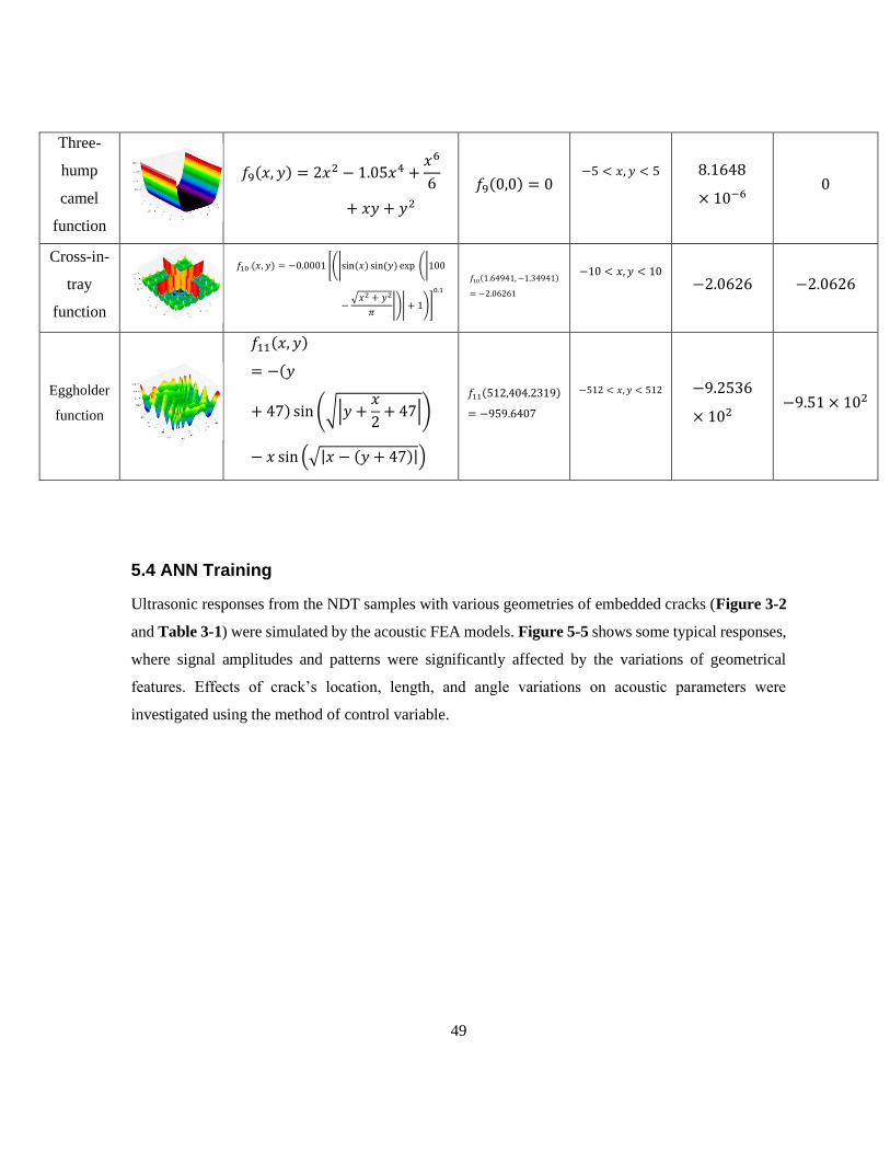
49
Three-
hump
camel
function
𝑓9(𝑥, 𝑦) = 2𝑥2 − 1.05𝑥4 +𝑥6
6
+ 𝑥𝑦 + 𝑦2
𝑓9(0,0) = 0 −5 < 𝑥, 𝑦 < 5
8.1648
× 10−6 0
Cross-in-
tray
function
𝑓10 (𝑥, 𝑦) = −0.0001 [(|sin(𝑥) sin(𝑦) exp (|100
−√𝑥2 + 𝑦2
𝜋|)| + 1)]
0.1
𝑓10(1.64941, −1.34941)
= −2.06261
−10 < 𝑥, 𝑦 < 10
−2.0626 −2.0626
Eggholder
function
𝑓11(𝑥, 𝑦)
= −(𝑦
+ 47) sin (√|𝑦 +𝑥
2+ 47|)
− 𝑥 sin (√|𝑥 − (𝑦 + 47)|)
𝑓11(512,404.2319)
= −959.6407
−512 < 𝑥, 𝑦 < 512
−9.2536
× 102 −9.51 × 10²
5.4 ANN Training
Ultrasonic responses from the NDT samples with various geometries of embedded cracks (Figure 3-2
and Table 3-1) were simulated by the acoustic FEA models. Figure 5-5 shows some typical responses,
where signal amplitudes and patterns were significantly affected by the variations of geometrical
features. Effects of crack’s location, length, and angle variations on acoustic parameters were
investigated using the method of control variable.

50
Figure 5-5 Ultrasonic responses to the variations of location, length, and angle of the embedded
crack produced by acoustic FEA models.
The boxplots in Figure 5-6 show the minimum, maximum, percentiles, and median values of the
normalized values of 24 parameters in Equation 3-4. In each box, the central mark is the median, the
edges of the box are the 25th and 75th percentiles, and the whiskers represent data outside the upper
and lower quartiles which were not considered for ANN training. Wide distribution of input dataset can
result in a high performance of the network. The plot shows that distribution of all 𝑏1 and 𝑐1 values for
525 training samples are compact while 𝑎2, 𝑏5, and 𝑏7 distributions are quite loose. Moreover, while
𝑎5, 𝑎7, and 𝑎8 have highest normal distribution, 𝑎6, 𝑐1 and 𝑏5 have the least.

51
Figure 5-6 Boxplots of normalized acoustic inputs for the neural network.
5.5 ANN Testing
The proposed FFNN was trained by TEA (FFNNTEA) to estimate crack geometrical features. In
FFNNTEA, number of input nodes was set to 6, hidden nodes to 10, and two nodes in the output layer.
The weights of network in training phase were considered as variables of the optimization problem.
Mean Square Error (MSE) was used as a cost function in TEA. The FFNNTEA weights was initialized
randomly and served as initial systems for the TEA to optimize the error cost function.
After training, the network was tested using the testing dataset. The testing dataset was not revealed
to the network during the training process, but was fed to the network after the training to estimate the
geometrical features corresponding to the given ultrasonic signal. The outputs from the network were
compared with desired values, and the discrepancy was calculated.
Performance evaluations of the proposed ANN was accomplished through the comparisons between
estimated and desired geometrical features for all 750 datasets. In Figure 5-7, geometrical features of
the crack are plotted with respect to the corresponding test number for FFNNTEA model.
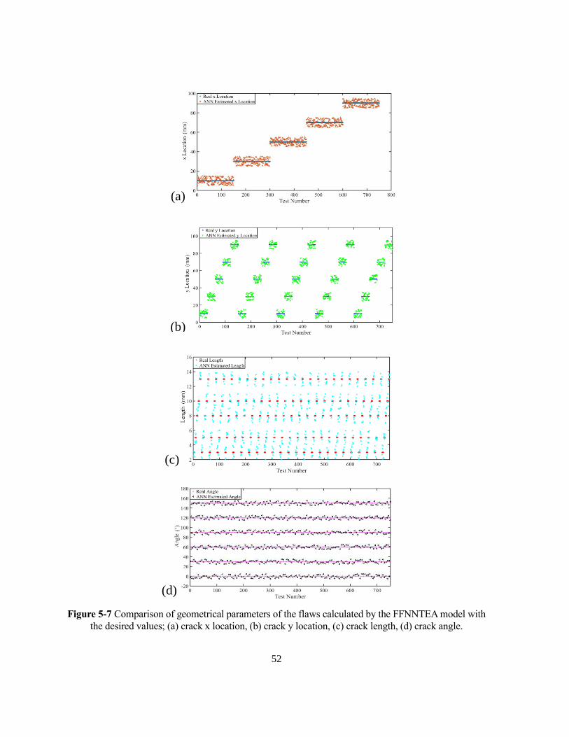
52
Figure 5-7 Comparison of geometrical parameters of the flaws calculated by the FFNNTEA model with
the desired values; (a) crack x location, (b) crack y location, (c) crack length, (d) crack angle.
(a)
(b)
(c)
(d)

53
Variations of the estimated values of crack location, length, and angle from the ANN models against
the desired ones are plotted in Figure 5-8. All the plots in Figure 5-8 demonstrate highly linear
relationship between them. To compare the performance of the network in location, length, and angle
estimations, the regression coefficients were measured for all datasets. Table 5-3 presents linear
regression coefficients, including slopes and intercepts of the fitted lines for feed-forward back-
propagation (FFBP) and FFNNTEA.
Figure 5-8 Regression analysis performed over the crack location, length, and angle estimations
calculated by ANN model.
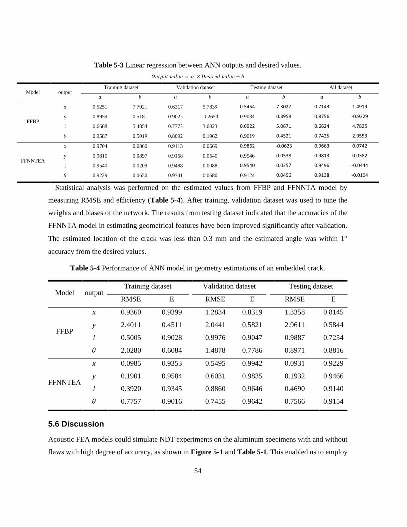
54
Table 5-3 Linear regression between ANN outputs and desired values.
𝑂𝑢𝑡𝑝𝑢𝑡 𝑣𝑎𝑙𝑢𝑒 = 𝑎 × 𝐷𝑒𝑠𝑖𝑟𝑒𝑑 𝑣𝑎𝑙𝑢𝑒 + 𝑏
Model output Training dataset Validation dataset Testing dataset All dataset
𝑎 𝑏 𝑎 𝑏 𝑎 𝑏 𝑎 𝑏
FFBP
x 0.5251 7.7021 0.6217 5.7839 0.5454 7.3027 0.7143 1.4919
y 0.8959 0.5181 0.9025 -0.2654 0.9034 0.3958 0.8756 -0.9329
l 0.6688 5.4854 0.7773 3.6023 0.6922 5.0671 0.6624 4.7825
𝜃 0.9587 0.5019 0.8092 0.1962 0.9019 0.4521 0.7425 2.9553
FFNNTEA
x 0.9704 0.0860 0.9113 0.0669 0.9862 -0.0623 0.9663 0.0742
y 0.9815 0.0897 0.9158 0.0540 0.9546 0.0538 0.9813 0.0382
l 0.9540 0.0209 0.9488 0.0088 0.9540 0.0257 0.9496 -0.0444
𝜃 0.9229 0.0650 0.9741 0.0680 0.9124 0.0496 0.9138 -0.0104
Statistical analysis was performed on the estimated values from FFBP and FFNNTA model by
measuring RMSE and efficiency (Table 5-4). After training, validation dataset was used to tune the
weights and biases of the network. The results from testing dataset indicated that the accuracies of the
FFNNTA model in estimating geometrical features have been improved significantly after validation.
The estimated location of the crack was less than 0.3 mm and the estimated angle was within 1
accuracy from the desired values.
Table 5-4 Performance of ANN model in geometry estimations of an embedded crack.
Model output Training dataset Validation dataset Testing dataset
RMSE E RMSE E RMSE E
FFBP
x 0.9360 0.9399 1.2834 0.8319 1.3358 0.8145
y 2.4011 0.4511 2.0441 0.5821 2.9611 0.5844
l 0.5005 0.9028 0.9976 0.9047 0.9887 0.7254
𝜃 2.0280 0.6084 1.4878 0.7786 0.8971 0.8816
FFNNTEA
x 0.0985 0.9353 0.5495 0.9942 0.0931 0.9229
y 0.1901 0.9584 0.6031 0.9835 0.1932 0.9466
l 0.3920 0.9345 0.8860 0.9646 0.4690 0.9140
𝜃 0.7757 0.9016 0.7455 0.9642 0.7566 0.9154
5.6 Discussion
Acoustic FEA models could simulate NDT experiments on the aluminum specimens with and without
flaws with high degree of accuracy, as shown in Figure 5-1 and Table 5-1. This enabled us to employ
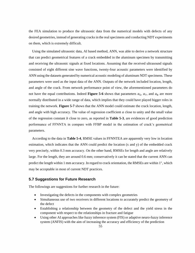
55
the FEA simulation to produce the ultrasonic data from the numerical models with defects of any
desired geometries, instead of generating cracks in the real specimens and conducting NDT experiments
on them, which is extremely difficult.
Using the simulated ultrasonic data, AI based method, ANN, was able to derive a network structure
that can predict geometrical features of a crack embedded in the aluminum specimen by transmitting
and receiving the ultrasonic signals at fixed locations. Assuming that the received ultrasound signals
consisted of eight different sine wave functions, twenty-four acoustic parameters were identified by
ANN using the datasets generated by numerical acoustic modeling of aluminum NDT specimens. These
parameters were used as the input data of the ANN. Outputs of the network included location, length,
and angle of the crack. From network performance point of view, the aforementioned parameters do
not have the equal contributions. Indeed Figure 5-6 shows that parameters 𝑎5, 𝑎7, and 𝑎8 are more
normally distributed in a wide range of data, which implies that they could have played bigger roles in
training the network. Figure 5-7 shows that the ANN model could estimate the crack location, length,
and angle with high accuracy. The value of regression coefficient 𝑎 close to unity and the small value
of the regression constant 𝑏 close to zero, as reported in Table 5-3, are evidences of good prediction
performance of FFNNTA in compare with FFBP model in the estimation of crack’s geometrical
parameters.
According to the data in Table 5-4, RMSE values in FFNNTEA are apparently very low in location
estimation, which indicates that the ANN could predict the location (x and y) of the embedded crack
very precisely, within 0.3 mm accuracy. On the other hand, RMSEs for length and angle are relatively
large. For the length, they are around 0.6 mm; conservatively it can be stated that the current ANN can
predict the length within 1 mm accuracy. In regard to crack orientation, the RMSEs are within 1, which
may be acceptable in most of current NDT practices.
5.7 Suggestions for Future Research
The followings are suggestions for further research in the future:
• Investigating the defects in the components with complex geometries
• Simultaneous use of two receivers in different locations to accurately predict the geometry of
the defect
• Establishing a relationship between the geometry of the defect and the yield stress in the
component with respect to the relationships in fracture and fatigue
• Using other AI approaches like fuzzy inference system (FIS) or adaptive neuro-fuzzy inference
system (ANFIS) with the aim of increasing the accuracy and efficiency of the prediction

56
Bibliography
[1] Charles Hellier (2003). Handbook of Nondestructive Evaluation. McGraw- Hill. p. 1.1.
[2] nde-ed.org NDT Education Resource Center
[3] Cartz, Louis (1995). Nondestructive Testing. A S M International.
[4] asnt.org Introduction to Nondestructive Testing.
[5] Bridges, Andrew. "High Speed Cameras for Non-Destructive Testing". NASA TechBriefs.
Retrieved 1 November 2013.
[6] Blitz, Jack; G. Simpson (1991). Ultrasonic Methods of Non-Destructive Testing. Springer-
Verlag New York, LLC.
[7] Waldmann, T. (2014). "A Mechanical Aging Mechanism in Lithium-Ion Batteries". Journal of
the Electrochemical Society. 161 (10): A1742–A1747.
[8] customers.phtool.com EDM Notch Reference Standards » PH Tool.
[9] customers.phtool.com Radiography (RT) Reference Standards » PH Tool.
[10] collections.ctdigitalarchive.org Connecticut Digital Archive | Connect. Preserve. Share
[11] "Today in History – Fales & Gray Explosion Underscores Need for a Hartford Hospital |
Connecticut History | a CTHumanities Project". Retrieved 2019-08-17.
[12] www.ndt-ed.org. History of PI.
[13] Singh S, Goyal A (2007). "The origin of echocardiography: a tribute to Inge Edler". Tex Heart
Inst J. 34 (4): 431–8.
[14] U.S. Patent 3,277,302, titled "X-Ray Apparatus Having Means for Supplying An Alternating
Square Wave Voltage to the X-Ray Tube", granted to Weighart on October 4, 1964, showing
its patent application date as May 10, 1963 and at lines 1-6 of its column 4, also, noting James
F. McNulty’s earlier filed co-pending application for an essential component of invention.
[15] R/D Tech Inc., “Introduction to phased array ultrasonic technology applications,” Olympus,
NDT Waltham, MA, 2007.
[16] K. Reber, M. Beller, N. I. Uzelac, How do defect assessment methods influence the choice and
construction of in-line inspection tools, Proc. of the 4th Int. Pipeline Conf., CD-ROM, Calgary,
2002.
[17] Matlack, K. H.; Kim, J.-Y.; Jacobs, L. J.; Qu, J. (2015-03-01). "Review of Second Harmonic
Generation Measurement Techniques for Material State Determination in Metals". Journal of
Nondestructive Evaluation. 34 (1): 273.
[18] Mostavi, Amir; Kamali, Negar; Tehrani, Niloofar; Chi, Sheng-Wei; Ozevin, Didem;
Indacochea, J. Ernesto (2017). "Wavelet Based Harmonics Decomposition of Ultrasonic Signal
in Assessment of Plastic Strain in Aluminum". Measurement. 106: 66–78.
[19] U.S. Patent 3,260,105 for Ultrasonic Testing Apparatus and Method to James F. McNulty at
lines 37-48 and 60-72 of Column 1 and lines 1-4 of Column 2.
[20] A. Sinclair, An analysis of ultrasonic frequency response for flaw detection: a technique review,
Materials Evaluation 43 6, pp. 879–883, 1989.
[21] L. Cartz, “Nondestructive testing,” ASM International, Materials Park, OH (United States),
1995.
[22] R/D Tech Inc., “Introduction to phased array ultrasonic technology applications,” Olympus, NDT Waltham, MA, 2007.

57
[23] K. H. Matlack, J. -Y. Kim, L. J. Jacobs, and J. Qu, “Review of second harmonic generation measurement techniques for material state determination in metals,” Journal of Nondestructive Evaluation, vol. 34, no. 1, pp. 273, 2015.
[24] A. Mostavi, N. Kamali, N. Tehrani, S. -W. Chi, D. Ozevin, and J. E. Indacochea, “Wavelet based hormonics decomposition of ultrasonic signal in assessment of plastic strain in aluminum,” Measurement, vol. 106, pp. 66–78, 2017.
[25] K. Reber, M. Beller, and N. I. Uzelac, “How do defect assessment methods influence the choice and construction of in-line inspection tools,” 2002 4th International Pipeline Conference, pp. 2039–2044, 2002.
[26] J. D. Achenbach, “Quantitative nondestructive evaluation,” International Journal of Solids and Structures, vol. 37, no. 1-2, pp. 13–27, 2000.
[27] S. Chatillon, G. Cattiaux, M. Serre, and O. Roy, “An ultrasonic system for the inspection of
components with irregular geometry using a flexible phased array contact transducer and
released processing algorithms,” AIP Conference Proceedings, vol. 509, no. 1, pp. 1095–1102,
2000.
[28] B. Chassignole, R. El Guerjouma, M. -A. Ploix, and T. Fouquet, “Ultrasonic and structural
characterization of anisotropic austenitic stainless steel welds: towards a higher reliability in
ultrasonic non-destructive testing,” NDT & E International, vol. 43, no. 4, p. 273–282, 2010.
[29] L. Le Jeune, S. Robert, E. L. Villaverde, and C. Prada, “Plane wave imaging for ultrasonic non-
destructive testing: generalization to multimodal imaging,” Ultrasonics, vol. 64, pp. 128–138,
2016.
[30] M. Sutcliffe, M. Weston, B. Dutton, P. Charlton, and K. Donne, “Real-time full matrix capture
for ultrasonic non-destructive testing with acceleration of post-processing through graphic
hardware,” NDT & E International, vol. 51, pp. 16–23, 2012.
[31] J. H. Charles, “Handbook of nondestructive evaluation,” 2003.
[32] http://www.asnt.org © 2019 The American Society for NDT, Inc.
[33] J. K. Singh, and S. K. Bhardwaj, “Non destructive testing of welded metals to enhance the quality
of materials,” International Journal of Technical Research and Applications, vol. 3, no. 3, pp.
47–51, 2015.
[34] T. Rymarczyk, G. Klosowski, and E. Kozlowski, “A non-destructive system based on electrical
tomography and machine learning to analyze the moisture of buldings,” Sensors, vol. 18, no. 7,
pp. 2285, 2018.
[35] Simas Filho, E.F.; Souza, Y.N.; Lopes, J.L.; Farias, C.T.; Albuquerque, M.C. Decision support
system for ultrasound inspection of fiber metal laminates using statistical signal processing and
neural networks. Ultrasonics 2013, 53, 1104–1111.
[36] Simas Filho, E.F.; Silva, M.M., Jr.; Farias, P.C.; Albuquerque, M.C.; Silva, I.C.; Farias, C.T.
Flexible decision support system for ultrasound evaluation of fiber–metal laminates implemented
in a DSP. NDT E Int. 2016, 79, 38–45.
[37] Cruz, F.C.; Simas Filho, E.F.; Albuquerque, M.C.; Silva, I.C.; Farias, C.T.; Gouvea, L.L.
Efficient feature selection for neural network based detection of flaws in steel welded joints using
ultrasound testing. Ultrasonics 2017, 73, 1–8.
[38] H. Cai, C. Xu, S. Zhou, H. Yan, and L. Yang, “study on the thick-walled pipe ultrasonic signal
enhancement of modified S-transform and singular value decomposition,” Mathematical
Problems in Engineering, vol. 2015, 2015.
[39] Kesharaju, M.; Nagarajah, R. Feature selection for neural network based defect classification of
ceramic components using high frequency ultrasound. Ultrasonics 2015, 62, 271–277.

58
[40] Lawson, S.W.; Parker, G.A. Automatic detection of defects in industrial ultrasound images using
a neural network. (2 November 2018).
[41] Simone, G., et al. "Feature extraction techniques for ultrasonic signal classification."
International Journal of Applied Electromagnetics and Mechanics 15.1-4 (2002): 291-294.
[42] Meng, Min, et al. "Ultrasonic signal classification and imaging system for composite materials via deep convolutional neural networks." Neurocomputing 257 (2017): 128-135.
[43] Sarkar, Soumalya, et al. "Deep learning for structural health monitoring: A damage characterization application." Annual conference of the prognostics and health management society. 2016.
[44] S. Sambath, P. Nagaraj, N. Selvakumar, S. Arunachalam, and T. Page, “Automatic detection of defects in ultrasonic testing using artificial neural network,” International Journal of Microstructure and Materials Properties, vol. 5, no. 6, pp. 561–574, 2010.
[45] Ye, Jiaxing, Shunya Ito, and Nobuyuki Toyama. "Computerized ultrasonic imaging inspection: From shallow to deep learning." Sensors 18.11 (2018): 3820.
[46] A. Toghroli, E. Darvishmoghaddam, E. Zandi, Y. Parvan, M. Safa, M. Abdullahi, M. Mohammed, A. Heydari, K. Wakil, S. A. Gebreel, and M. Khorami, “Evaluation of the parameters affecting the Schmidt rebound hammer reading using ANFIS method,” Computers and Concrete, vol. 21, no. 5, pp. 525–530, 2018.
[47] N. Munir, H. J. Kim, S. J. Song, and S. S. Kang, “Investigation of deep neural network with drop out for ultrasonic flaw classification in weldments,” Journal of Mechanical Science and Technology, vol. 32, no. 7, pp. 3073–3080, 2018.
[48] Darmon, M., et al. "Recent advances in semi-analytical scattering models for NDT simulation." Journal of Physics: Conference Series. Vol. 269. No. 1. IOP Publishing, 2011.
[49] J.D. Achenbach, A.K. Gautesen, H. McMaken, Rays methods for waves in elastic solids, Pitman, 1982.
[50] P.Y. Ufimtsev, Fundamentals of the Physical Theory of Diffraction, John Wiley & Sons, 2007. [51] Darmon, M., et al. "A system model for ultrasonic NDT based on the Physical Theory of
Diffraction (PTD)." Ultrasonics 64 (2016): 115-127. [52] Zou, Cheng, et al. "Detection of longitudinal cracks with a serrated columnar phased array
transducer: A simulation study." 2015 International Conference on Control, Automation and Robotics. IEEE, 2015.
[53] P. Q. Tian, Y. W. Feng, S. Z. Zhan, X. Zhang, and X. Xue , “Numerical simulation of ultrasonic testing reliability of civil aircraft considering the influence of the angle between the sound beam axis and the crack orientation”, IOP Conference Series: Materials Science and Engineering. vol. 715, no. 1, pp. 012012, 2020.
[54] Owowo, Julius, and S. Olutunde Oyadiji. "Finite element analysis and experimental measurement of acoustic wave propagation for leakage detection in an air-filled pipe." International Journal of Structural Integrity (2017).
[55] Kroumov, Valeri, Jianli Yu, and Keishi Shibayama. "3D path planning for mobile robots using simulated annealing neural network." International Journal of Innovative Computing, Information and Control 6, no. 7 (2010): 2885-2899.
[56] Niaki, Seyed Taghi Akhavan, and Shirin Akbari Nasaji. "A hybrid method of artificial neural
networks and simulated annealing in monitoring auto-correlated multi-attribute processes." The
International Journal of Advanced Manufacturing Technology 56, no. 5-8 (2011): 777-788. [57] Yang, Shih-Hung, and Yon-Ping Chen. "An evolutionary constructive and pruning algorithm for
artificial neural networks and its prediction applications." Neurocomputing 86 (2012): 140-149.
[58] M.A. Ahmadi, Neural Network based unified particle swarm optimization for prediction
of asphaltene precipitation, Fluid Phase Equilibria 314 (2012) 46–51.

59
[59] Köker, Raşit. "A genetic algorithm approach to a neural-network-based inverse kinematics solution of robotic manipulators based on error minimization." Information Sciences 222 (2013): 528-543.
[60] Man, Kim-Fung, Kit-Sang Tang, and Sam Kwong. "Genetic algorithms: concepts and applications." IEEE Transactions on Industrial Electronics 43, no. 5 (1996): 519-534.
[61] Rashed, G. I., H. I. Shaheen, X. Z. Duan, and S. J. Cheng. "Evolutionary optimization techniques
for optimal location and parameter setting of TCSC under single line contingency." Applied
Mathematics and Computation 205, no. 1 (2008): 133-147. [62] X.He, J.Zeng, J.Jie, “Artificial neural network weights optimization design based on MEC
algorithm”, Proc. Of 2004 Intl. Conf. on Machine Learning and Cybernetics, Vol. 6, Aug. 2004, pp. 3361 – 3364.
[63] K. Hornik, M. Stinchocombe, and H. White, “Multilayer feedforward networks are universal
approximators,” Neural networks, vol. 2, pp. 359-366, 1989.