Assessment and Validation of Machine Learning Methods forPredicting Molecular Atomization EnergiesKatja Hansen,*,† Gregoire Montavon,‡ Franziska Biegler,‡ Siamac Fazli,‡ Matthias Rupp,¶

Matthias Scheffler,† O. Anatole von Lilienfeld,§ Alexandre Tkatchenko,† and Klaus-Robert Muller*,‡,∥

†Fritz-Haber-Institut der Max-Planck-Gesellschaft, Berlin, Germany‡Machine Learning Group, TU Berlin, Germany¶Institute of Pharmaceutical Sciences, ETH Zurich, Switzerland§Argonne Leadership Computing Facility, Argonne National Laboratory, Lemont, Illinois, United States∥Department of Brain and Cognitive Engineering, Korea University, Korea

*S Supporting Information

ABSTRACT: The accurate and reliable prediction of properties of molecules typically requires computationally intensivequantum-chemical calculations. Recently, machine learning techniques applied to ab initio calculations have been proposed as anefficient approach for describing the energies of molecules in their given ground-state structure throughout chemical compoundspace (Rupp et al. Phys. Rev. Lett. 2012, 108, 058301). In this paper we outline a number of established machine learningtechniques and investigate the influence of the molecular representation on the methods performance. The best methods achieveprediction errors of 3 kcal/mol for the atomization energies of a wide variety of molecules. Rationales for this performanceimprovement are given together with pitfalls and challenges when applying machine learning approaches to the prediction ofquantum-mechanical observables.

1. INTRODUCTION

The accurate prediction of molecular properties in chemicalcompound space (CCS) is a crucial ingredient toward rationalcompound design in chemical and pharmaceutical industries.Therefore, one of the major challenges is to enable quantitativecalculations of molecular properties in CCS at moderatecomputational cost (milliseconds per molecule or faster).However, currently only high level quantum-chemical calcu-lations, which can take up to several days per molecule, yieldthe desired “chemical accuracy” (e.g., 1 kcal/mol for molecularatomization energies) required for predictive in silico rationalmolecular design. Therefore, more efficient algorithms that canpredict properties of molecules quickly and reliably would be apowerful tool in order to sample and better understand CCS.Throughout this paper, we focus on atomization energies of

molecules in their ground-state equilibrium geometry. Theatomization energy is an essential molecular property thatdetermines the stability of a molecule with respect to the atomsthat compose it. Atomization energies are also measurable

experimentally and are frequently used to assess the perform-ance of approximate computational methods. Though we focuson atomization energies the methods described in this papercould also be applied to predict total molecular energies ordifferent quantum-mechanical properties.1

Recently, a machine learning (ML) approach has beendemonstrated to predict atomization energies of various smallmolecules in their given ground-state geometry.2 The methoduses the same input as electronic-structure calculations, namelynuclear charges and atomic positions, and learns from a trainingset of ab initio molecular energies. Though the authors showthat their proposed kernel ridge regression approach (detailswill be discussed below) outperforms the semiempirical PM63

and a simple bond-counting4 scheme, the question ariseswhether other molecular descriptors or machine learningmethods, e.g. neural networks, which have been successfully

Received: March 12, 2013

Article

pubs.acs.org/JCTC

© XXXX American Chemical Society A dx.doi.org/10.1021/ct400195d | J. Chem. Theory Comput. XXXX, XXX, XXX−XXX

applied for potential-energy surface (PES) description,5 are alsoor even better suited for predicting atomization energies.Let us briefly comment on the terminology. The term

“model” here refers to a function trained on a set of molecules(training set) that returns a property value for a givenmolecule.6 The term “prediction” refers to the fact that sucha model is able to predict properties of molecules that were notused to fit the model parameters. We note, however, that thepresented models are neither derived from nor explicitly basedon physical laws. Purely data-driven machine learningalgorithms are used to generate them. Thus, for moleculesthat behave significantly different than those of the training set,the prediction is likely to fail; the model may however assessthe probability for own errors.7 For example, when the trainingset would not contain first-row elements, the prediction ofproperties of first-row elements may not work, and, if thetraining set does not contain 3d transition metals, a failure forthese elements is also to be expected. On the other handpredictions can in principle work even when the underlyingphysical laws are (still) unknown. Thus, the methods describedbelow enable us to generate predictions for properties of a hugenumber of molecules that are unknown to the algorithm, butthey must not be qualitatively distinct from the molecules ofthe training set.In this work we show how significant improvements in the

prediction of atomization energies can be achieved by usingmore specific and suitable ML approaches compared to the onepresented by Rupp et al.2 We review several standard MLtechniques and analyze their performance, scaling, and handlingof atomization-energy prediction with respect to differentrepresentations of molecular data. Our best methods reduce theprediction error from 10 kcal/mol2 to 3 kcal/mol.These explicit ML models for learning molecular energies

have only been introduced recently. We therefore provide inthis paper comprehensive instructions for the best practical useof this novel tool set. If model selection and validation are notcarried out properly, overly optimistic or in the worst casesimply useless results may be obtained. A number of commonpitfalls are outlined to help avoid this situation.In cheminformatics, ML has been used extensively to

describe experimentally determined biochemical or physico-chemical molecular properties such as in quantitativestructure−activity relationships and quantitative structure−property relationships (e.g., refs 8−10). Since the 1990s neuralnetworks have been proposed to model first-principlescalculations for variable geometry.5,11−20 Most of them arelimited to fixed molecular compositions or systems with only afew different atom types. More recently, Gaussian processesand kernel ridge regression models were also applied to predictatomic multipole moments,21 the PES of solids,22 transition-state dividing surfaces,23 and exchange-correlation function-als.24 Hautier et al.25 used machine learning techniques tosuggest new crystal structures in order to explore the space ofternary oxides, while Balabin and Lomakina26,27 applied neuralnetworks and support vector machines to predict energies oforganic molecules. The latter considered molecular descriptorsand DFT energies calculated with small basis sets to predictDFT energies calculated with large basis sets. Most of thesemodels either partition the energy and construct separatemodels for local atom environments or represent the wholemolecule at once.In this work we explore methods which consider whole

chemical compounds at once to learn atomization energies of

molecules across chemical compound space. Much work hasbeen done (with and without ML) to describe nonequilibriumgeometries and understand potential-energy surfaces of variousmolecular systems. However, due to the unmanageable size ofCCS it is impossible to do QM calculations on large moleculardatabases. One also needs methods that can extend theaccuracy of first-principles QM methods across CCS. Our workis aiming toward this perspective.Note that we therefore restrict ourselves in this attempt to

ground-state geometries and focus on enlarging the numberand diversity of included systems. The incorporation ofnonequilibrium geometries is the subject of ongoing work.

2. DATA SET AND DATA REPRESENTATIONIn this section we describe the data set that is used to build andvalidate the ML models for atomization energy prediction. Thequality and applicability of ML prediction models inherentlydepend on the size and diversity of this underlying data set.Moreover, the numerical representation of the includedmolecular structures is a critical aspect for model quality.Three different representations are introduced in this sectionand further discussed in Section 5.

2.1. Data Set. The chemical database GDB-13 contains allmolecules obeying simple chemical rules for stability andsynthetic feasibility up to 13 first- and second-row atoms of C,N, O, S, and Cl (970 million compounds).28 In this work, as inRupp et al.,2 the subset formed by all molecules up to sevenfirst- and second-row atoms of C, N, O, and S is extracted fromthe GDB-13. This data set contains 7165 structures with amaximal size of 23 atoms per molecule (including hydrogens).The GDB-13 gives bonding information in the form ofSMILES29 strings. These are converted to Cartesiancoordinates of the ground-state structure using the OpenBabelimplementation30 of the force-field method by Rappe et al.31The atomization energies, which range from −800 to −2000kcal/mol, are then calculated for each molecule using thePerdew-Burke-Ernzerhof hybrid functional (PBE0).32,33 Thesesingle point calculations of geometry optimization wereperformed with a well converged numerical basis, asimplemented in the FHI-aims code34 (tight settings/tier2basis set).

2.2. Data Representation. In order to apply machinelearning, the information encoded in the molecular three-dimensional structure needs to be converted into anappropriate vector of numbers. This vectorial representationof a molecule is very important for the success of the learningapproach. Only if all information relevant for the atomizationenergy is appropriately encoded in the vector will the machinelearning algorithm be able to infer the relation betweenmolecules and atomization energies correctly. Our representa-tion should be solely based on atomic coordinates Ri andnuclear charges Zi, as we want to pursue an approach from firstprinciples that can deal with any stoichiometry and atomicconfiguration.Different system representations that include internal

coordinates, system-specific variables, and complex projectionsof local atom densities have been proposed in the context ofpotential-energy prediction.22,5 Finding the optimal representa-tion for molecules is the subject of ongoing research, and an in-depth discussion of all of them would be beyond the scope ofthis work. Therefore, we focus on three representations derivedfrom the Coulomb matrix C, a simple matrix representationintroduced by Rupp et al.2 (Figure 1).

Journal of Chemical Theory and Computation Article

dx.doi.org/10.1021/ct400195d | J. Chem. Theory Comput. XXXX, XXX, XXX−XXXB

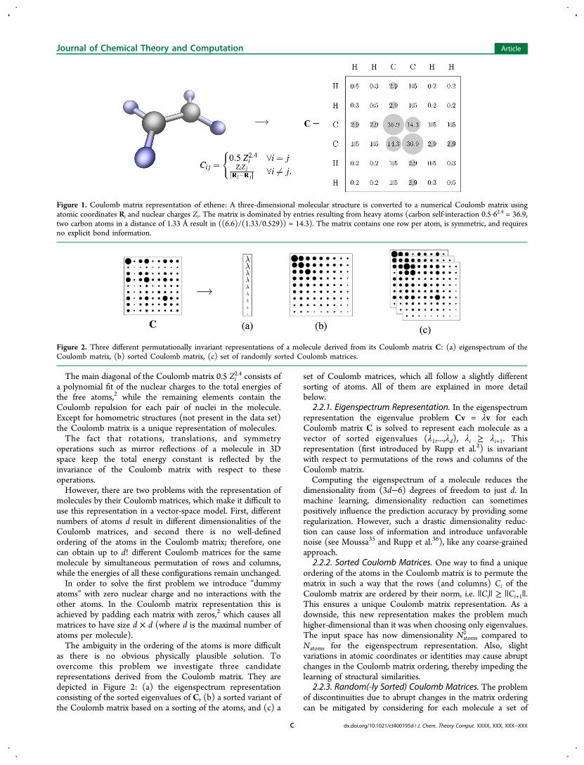
The main diagonal of the Coulomb matrix 0.5 Zi2.4 consists of

a polynomial fit of the nuclear charges to the total energies ofthe free atoms,2 while the remaining elements contain theCoulomb repulsion for each pair of nuclei in the molecule.Except for homometric structures (not present in the data set)the Coulomb matrix is a unique representation of molecules.The fact that rotations, translations, and symmetry

operations such as mirror reflections of a molecule in 3Dspace keep the total energy constant is reflected by theinvariance of the Coulomb matrix with respect to theseoperations.However, there are two problems with the representation of

molecules by their Coulomb matrices, which make it difficult touse this representation in a vector-space model. First, differentnumbers of atoms d result in different dimensionalities of theCoulomb matrices, and second there is no well-definedordering of the atoms in the Coulomb matrix; therefore, onecan obtain up to d! different Coulomb matrices for the samemolecule by simultaneous permutation of rows and columns,while the energies of all these configurations remain unchanged.In order to solve the first problem we introduce “dummy

atoms” with zero nuclear charge and no interactions with theother atoms. In the Coulomb matrix representation this isachieved by padding each matrix with zeros,2 which causes allmatrices to have size d × d (where d is the maximal number ofatoms per molecule).The ambiguity in the ordering of the atoms is more difficult

as there is no obvious physically plausible solution. Toovercome this problem we investigate three candidaterepresentations derived from the Coulomb matrix. They aredepicted in Figure 2: (a) the eigenspectrum representationconsisting of the sorted eigenvalues of C, (b) a sorted variant ofthe Coulomb matrix based on a sorting of the atoms, and (c) a

set of Coulomb matrices, which all follow a slightly differentsorting of atoms. All of them are explained in more detailbelow.

2.2.1. Eigenspectrum Representation. In the eigenspectrumrepresentation the eigenvalue problem Cv = λv for eachCoulomb matrix C is solved to represent each molecule as avector of sorted eigenvalues (λ1,...,λd), λi ≥ λi+1. Thisrepresentation (first introduced by Rupp et al.2) is invariantwith respect to permutations of the rows and columns of theCoulomb matrix.Computing the eigenspectrum of a molecule reduces the

dimensionality from (3d−6) degrees of freedom to just d. Inmachine learning, dimensionality reduction can sometimespositively influence the prediction accuracy by providing someregularization. However, such a drastic dimensionality reduc-tion can cause loss of information and introduce unfavorablenoise (see Moussa35 and Rupp et al.36), like any coarse-grainedapproach.

2.2.2. Sorted Coulomb Matrices. One way to find a uniqueordering of the atoms in the Coulomb matrix is to permute thematrix in such a way that the rows (and columns) Ci of theCoulomb matrix are ordered by their norm, i.e. ||Ci|| ≥ ||Ci+1||.This ensures a unique Coulomb matrix representation. As adownside, this new representation makes the problem muchhigher-dimensional than it was when choosing only eigenvalues.The input space has now dimensionality Natoms

2 compared toNatoms for the eigenspectrum representation. Also, slightvariations in atomic coordinates or identities may cause abruptchanges in the Coulomb matrix ordering, thereby impeding thelearning of structural similarities.

2.2.3. Random(-ly Sorted) Coulomb Matrices. The problemof discontinuities due to abrupt changes in the matrix orderingcan be mitigated by considering for each molecule a set of

Figure 1. Coulomb matrix representation of ethene: A three-dimensional molecular structure is converted to a numerical Coulomb matrix usingatomic coordinates Ri and nuclear charges Zi. The matrix is dominated by entries resulting from heavy atoms (carbon self-interaction 0.5·62.4 = 36.9,two carbon atoms in a distance of 1.33 Å result in ((6.6)/(1.33/0.529)) = 14.3). The matrix contains one row per atom, is symmetric, and requiresno explicit bond information.

Figure 2. Three different permutationally invariant representations of a molecule derived from its Coulomb matrix C: (a) eigenspectrum of theCoulomb matrix, (b) sorted Coulomb matrix, (c) set of randomly sorted Coulomb matrices.

Journal of Chemical Theory and Computation Article

dx.doi.org/10.1021/ct400195d | J. Chem. Theory Comput. XXXX, XXX, XXX−XXXC

Coulomb matrices rather than a single sorted Coulombmatrix.37 To generate these randomly sorted Coulomb matriceswe construct the Coulomb matrix based on a random orderingof the atoms and compute the row norms ||C|| (i.e., a vectorcontaining the norm of each row of Ci). We add random noiseε ∼ (0,σI) to disturb the vector ||C|| and determine thepermutation P that sorts ||C||+ε. Finally, the rows and columnsof the Coulomb matrix C are permuted according to thispermutation, i.e. Crandom = permuterowsP(permutecolsP(C)).(Note that for no noise (σ = 0) this equals the sorted Coulombrepresentation described above.)This procedure corresponds to an approximate sampling

from the conditional distribution of all possible valid Coulombmatrices given a specific molecule.37 Similar approaches havebeen used in a variety of contexts, for example, feedingelastically distorted handwritten digits to a neural network38,39

or a support vector machine,40 leading to dramatic performanceimprovements.Note that the increased number of samples caused by

considering a set of random Coulomb matrices for eachmolecule helps to overcome the high-dimensionality of theinput space but also considerably increases the computationalcosts for some ML methods. We discuss this problem inSection 4.2.2.

3. MACHINE LEARNING METHODS

Machine learning (ML) seeks to infer dependencies from datausing computing systems with learning capability. This subfieldof artificial intelligence evolved in the 1950s from theintersection of computer science, statistics, and neuroscienceand gave rise to various learning algorithms commonly used inbioinformatics, computer vision, speech recognition, andfinance.41−47

In this paper we focus on the description of atomizationenergies of molecules in their ground-state structures. From amathematical point of view this is a regression task: We seek tofind a function or model f ∈ that maps an input vector x ∈d (representing the molecule: nuclear number and position ofall atoms) onto the corresponding continuous label value y ∈ (here the atomization energy). The space of functionsdepends on the employed machine learning method andincorporated additional information and assumptions. Since weconsider a training data set {(x1,y1),...,(xn,yn)} in order to find f∈ , the task falls into the category of supervised learning. TheML problem is formulated as a minimization problem of theform

∑ λ+ ∈=

f y r f fxmin ( ( ), ) ( ) withf i

n

i i1 (1)

The first term of the objective is the empirical risk described bya loss function which measures the quality of the function f. Aspecific case is the squared loss = −y y y y( , ) ( )2. Somecommon loss functions are given in Table 1. The second termof the objective in eq 1 is a regularization term which measuresthe complexity or roughness of the function f. In general r( f) isa norm of f or its derivatives, e.g. ∫ f″(x)2dx can be used tofavor functions that vary slowly over small regions of inputspace. The interplay between these two terms can beinterpreted as follows: Among all functions f that predict outputsy f rom inputs x well, choose the one that is the least complex.In addition to the need to carefully design the complexity

penalty λr( f), we also need to make sure that the space offunctions contains enough functions that can approximatethe physical dependencies between molecular structures andatomization energies. The atomization energy results from thequantum mechanical interactions between many electrons.Thus we expect a function that reasonably approximatesatomization energies to be complex and highly nonlinear. Inthis work the effect of the considered space of functions on thequality of the approximation is illustrated by moving from thespace of linear functions to nonlinear differentiable functions.The simultaneous need for sophisticated function classes

and appropriate regularizers r( f) underlies the design of all MLalgorithms. Learning algorithms that implement them in oneway or another are described in the following sections. For thesake of notational simplicity we will assume in the formulas thatthe data are centered, i.e. (1/n)Σi=1

n yi = 0 and (1/n)Σi=1n xi = 0.

The main differences of the regression methods discussed inthe following lie in two aspects, namely the set of candidatefunctions for f that are taken into account and the criteriaapplied to select the best candidate functions, i.e. the choice offunctionals and r.

3.1. Linear Ridge Regression. One of the simplest andmost popular regression models is least-squares linear regression,where the unknown function is approximated by the hyper-plane that minimizes the squared distance between thepredicted and the true function value. In ridge regression theobjective function of the least-squares linear regression model isextended by a regularizer to make the model less sensitive tooutliers. It reads in analogy to eq 1 as

∑ λ− + ·|| || ==n

y f fx w x x wmin1

( ( )) with ( )i

n

i iT

w1

2 2

(5)

for a given λ > 0. The minimization problem of eq 5 can besolved in closed form with w = (XTX+λI)−1XTy, where y is thetraining label vector, and X refers to the matrix of all inputvectors. This approach, in contrast to the following ones, islimited to the set of linear functions, i.e. only linear

Table 1. Selection of Loss Functions for Regression Tasksa

parameter comments

squared error loss = −y f y fx x( , ( )) ( ( ))i i i ise2

(2)

absolute error loss = | − |y f y fx x( , ( )) ( )i i i iae (3)

ε-insensitive loss

εε

= | − | = | − | −| − | ≤

ε ε ⎪

⎪⎧⎨⎩y f f y f y

if f y

otherwisex x

xx

( , ( )) ( )0

( )( )

i i i ii i

i i

(4)aThe squared error loss is the most commonly used. The absolute error compared to the squared error is more robust to outliers but notdifferentiable. The ε-insensitive loss leaves errors up to ε unpenalized and has the effect of introducing some slack (or looseness).

Journal of Chemical Theory and Computation Article

dx.doi.org/10.1021/ct400195d | J. Chem. Theory Comput. XXXX, XXX, XXX−XXXD

dependencies between molecules represented as vectors xi andtheir corresponding energies are captured.The regularization parameter λ controls the balance between

the quality of the fit (here measured using the squared loss) andthe complexity of the function. The parameter λ is a so-called“hyperparameter”. It is not determined within training (i.e.,solving the optimization problem eq 5) and needs to be chosenseparately within a so-called “model selection” procedure (cf.Section 4.1). In general, regularization is needed in order towork with noisy data, such as experimental measurements ofmolecular energies. However, in this work we aim to reproducethe results of an electronic structure calculation, and thesecalculated molecular energies include no noise up to numericalprecision. The concept of regularization is still beneficial inorder to focus on less complex solutions and to cope withambiguities in the representation of molecules. For example,based on the molecular representations introduced in Section2.2 two homometric molecular structures of different energyvalues are mapped onto exactly the same input vectors xi. Froman algorithmic perspective this situation could also result fromtwo noisy measurements of the same input. This ambiguity canbe handled using regularization.3.2. Kernel Ridge Regression. Kernel ridge regression

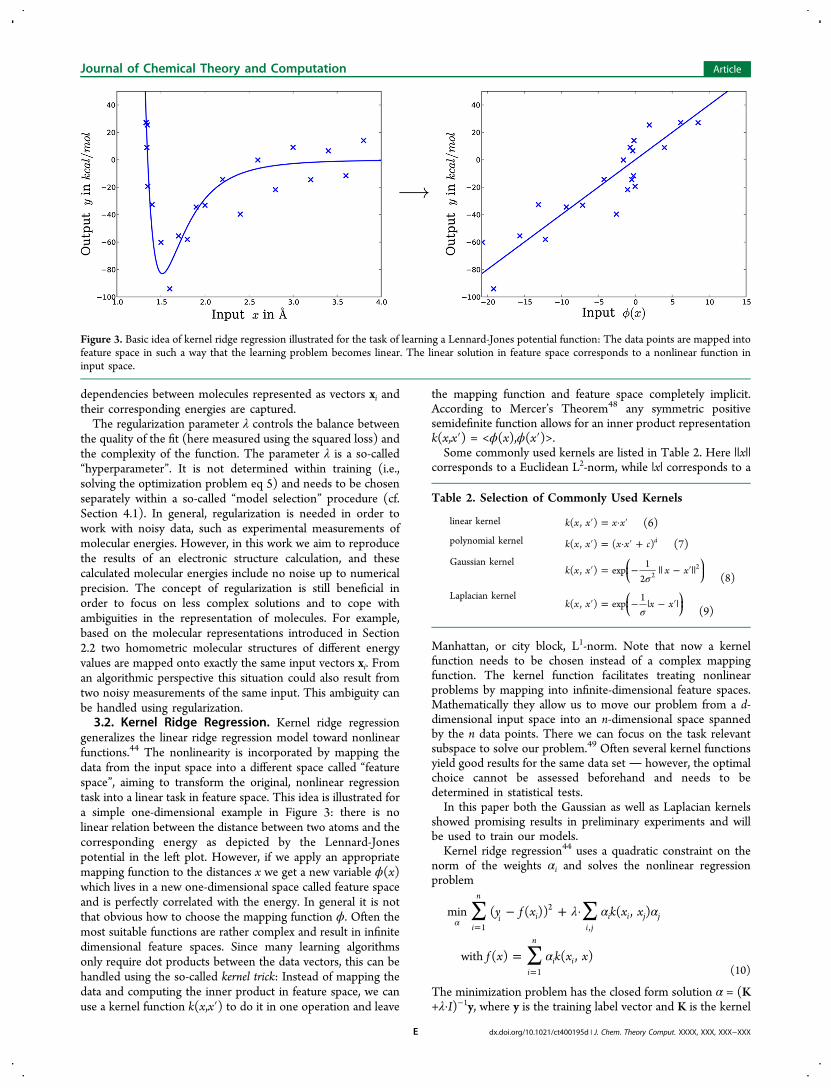
generalizes the linear ridge regression model toward nonlinearfunctions.44 The nonlinearity is incorporated by mapping thedata from the input space into a different space called “featurespace”, aiming to transform the original, nonlinear regressiontask into a linear task in feature space. This idea is illustrated fora simple one-dimensional example in Figure 3: there is nolinear relation between the distance between two atoms and thecorresponding energy as depicted by the Lennard-Jonespotential in the left plot. However, if we apply an appropriatemapping function to the distances x we get a new variable ϕ(x)which lives in a new one-dimensional space called feature spaceand is perfectly correlated with the energy. In general it is notthat obvious how to choose the mapping function ϕ. Often themost suitable functions are rather complex and result in infinitedimensional feature spaces. Since many learning algorithmsonly require dot products between the data vectors, this can behandled using the so-called kernel trick: Instead of mapping thedata and computing the inner product in feature space, we canuse a kernel function k(x,x′) to do it in one operation and leave

the mapping function and feature space completely implicit.According to Mercer’s Theorem48 any symmetric positivesemidefinite function allows for an inner product representationk(x,x′) = <ϕ(x),ϕ(x′)>.Some commonly used kernels are listed in Table 2. Here ||x||

corresponds to a Euclidean L2-norm, while |x| corresponds to a

Manhattan, or city block, L1-norm. Note that now a kernelfunction needs to be chosen instead of a complex mappingfunction. The kernel function facilitates treating nonlinearproblems by mapping into infinite-dimensional feature spaces.Mathematically they allow us to move our problem from a d-dimensional input space into an n-dimensional space spannedby the n data points. There we can focus on the task relevantsubspace to solve our problem.49 Often several kernel functionsyield good results for the same data set however, the optimalchoice cannot be assessed beforehand and needs to bedetermined in statistical tests.In this paper both the Gaussian as well as Laplacian kernels

showed promising results in preliminary experiments and willbe used to train our models.Kernel ridge regression44 uses a quadratic constraint on the

norm of the weights αi and solves the nonlinear regressionproblem

∑ ∑

∑

λ α α

α

− + ·

=

α =

=

y f x k x x

f x k x x

min ( ( )) ( , )

with ( ) ( , )

i

n

i ii j

i i j j

i

n

i i

1

2

,

1 (10)

The minimization problem has the closed form solution α = (K+λ·I)−1y, where y is the training label vector and K is the kernel

Figure 3. Basic idea of kernel ridge regression illustrated for the task of learning a Lennard-Jones potential function: The data points are mapped intofeature space in such a way that the learning problem becomes linear. The linear solution in feature space corresponds to a nonlinear function ininput space.

Table 2. Selection of Commonly Used Kernels

linear kernel ′ = · ′k x x x x( , ) (6)

polynomial kernel ′ = · ′ +k x x x x c( , ) ( )d (7)

Gaussian kernel

σ′ = − || − ′||⎜ ⎟⎛

⎝⎞⎠k x x x x( , ) exp

12 2

2

(8)

Laplacian kernel

σ′ = − | − ′|⎜ ⎟

⎛⎝

⎞⎠k x x x x( , ) exp

1(9)

Journal of Chemical Theory and Computation Article

dx.doi.org/10.1021/ct400195d | J. Chem. Theory Comput. XXXX, XXX, XXX−XXXE

matrix. The regularization parameter λ is again a hyper-parameter, as are any kernel dependent parameters, such as, inthe case of the Gaussian and Laplacian kernel, the kernel widthσ. They need to be chosen separately within a model selectionprocedure (cf. section 4.1).One main drawback of kernel-based methods such as kernel

ridge regression is that they are in general not well suited forlarge data sets. In our work this issue only arises when manyrandom Coulomb matrices are used to represent one molecule(see Section 4.2.2 for further discussion).3.3. Support Vector Regression. Support vector

regression (SVR)46,50,51 is a kernel-based regression method,which can be depicted as a linear regression in feature space −like kernel ridge regression. Unlike kernel ridge regression, SVRis based on an ε-insensitive loss function (eq 4), where absolutedeviations up to ε are tolerated.The corresponding convex optimization problem has a

unique solution, which cannot be written in a closed form but isdetermined efficiently using numerical methods for quadraticprogramming (see Chapter 10 of Scholkopf and Smola46 andPlatt52). One key feature of SVR is sparsity, i.e. only a few ofthe data points contribute to the solution. These are calledsupport vectors. Though the number of support vectors isgenerally small it may rise dramatically for very complex or verynoisy problems.43

For a given data set with n data points, SVR solves theoptimization problem

∑

∑ ∑

α α α α

ε α α α α

− − * − *

− + * + − *

α α*=

= =

k x x

y

max12

( )( ) ( , )

( ) ( ),

i j

n

i i j j i j

i

n

i ii

n

i i i

, , 1

1 1

i i

(11)

subject to the following constraints

∑ α α α α− * = ≤ * ≤=

C( ) 0 and 0 ,i

n

i i i i1 (12)

where C is a regularizing hyperparameter. The regressionfunction takes the form

∑ α α= − *=

f x k x x( ) ( ) ( , )i

n

i i i1 (13)

Based on preliminary experiments the Gaussian and Laplaciankernel were selected for the support vector regressionemployed in this study. Thus two hyperparameters need tobe optimized, namely the kernel width σ and the parameter C.

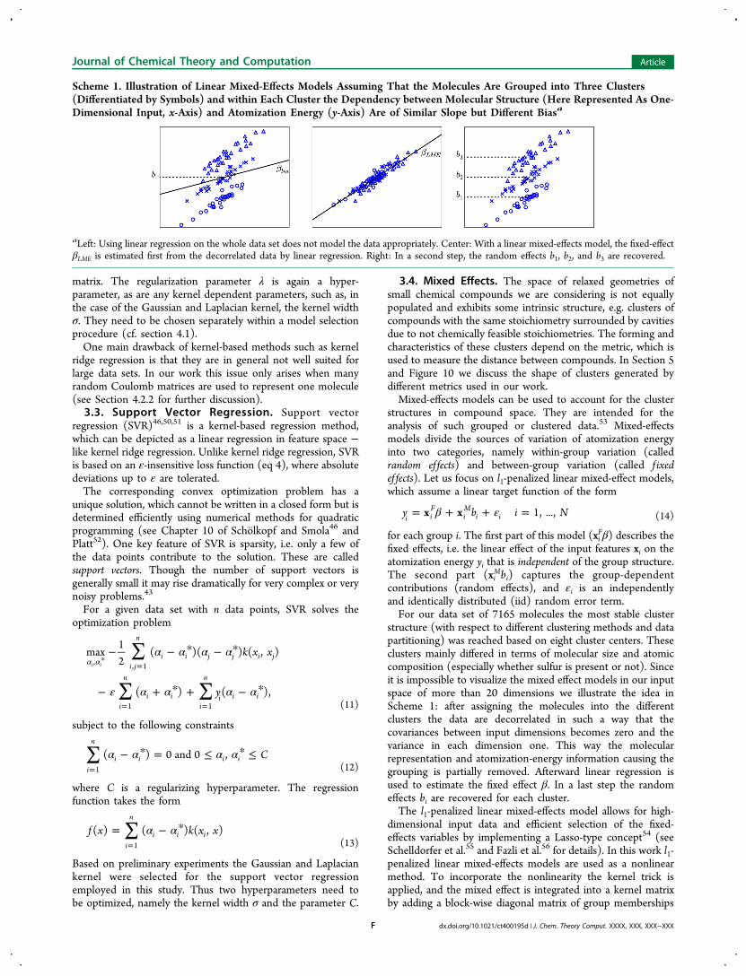
3.4. Mixed Effects. The space of relaxed geometries ofsmall chemical compounds we are considering is not equallypopulated and exhibits some intrinsic structure, e.g. clusters ofcompounds with the same stoichiometry surrounded by cavitiesdue to not chemically feasible stoichiometries. The forming andcharacteristics of these clusters depend on the metric, which isused to measure the distance between compounds. In Section 5and Figure 10 we discuss the shape of clusters generated bydifferent metrics used in our work.Mixed-effects models can be used to account for the cluster

structures in compound space. They are intended for theanalysis of such grouped or clustered data.53 Mixed-effectsmodels divide the sources of variation of atomization energyinto two categories, namely within-group variation (calledrandom ef fects) and between-group variation (called f ixedef fects). Let us focus on l1-penalized linear mixed-effect models,which assume a linear target function of the form

β ε= + + =y b i Nx x 1, ...,i iF

iM

i i (14)

for each group i. The first part of this model (xiFβ) describes the

fixed effects, i.e. the linear effect of the input features xi on theatomization energy yi that is independent of the group structure.The second part (xi

Mbi) captures the group-dependentcontributions (random effects), and εi is an independentlyand identically distributed (iid) random error term.For our data set of 7165 molecules the most stable cluster

structure (with respect to different clustering methods and datapartitioning) was reached based on eight cluster centers. Theseclusters mainly differed in terms of molecular size and atomiccomposition (especially whether sulfur is present or not). Sinceit is impossible to visualize the mixed effect models in our inputspace of more than 20 dimensions we illustrate the idea inScheme 1: after assigning the molecules into the differentclusters the data are decorrelated in such a way that thecovariances between input dimensions becomes zero and thevariance in each dimension one. This way the molecularrepresentation and atomization-energy information causing thegrouping is partially removed. Afterward linear regression isused to estimate the fixed effect β. In a last step the randomeffects bi are recovered for each cluster.The l1-penalized linear mixed-effects model allows for high-

dimensional input data and efficient selection of the fixed-effects variables by implementing a Lasso-type concept54 (seeSchelldorfer et al.55 and Fazli et al.56 for details). In this work l1-penalized linear mixed-effects models are used as a nonlinearmethod. To incorporate the nonlinearity the kernel trick isapplied, and the mixed effect is integrated into a kernel matrixby adding a block-wise diagonal matrix of group memberships

Scheme 1. Illustration of Linear Mixed-Effects Models Assuming That the Molecules Are Grouped into Three Clusters(Differentiated by Symbols) and within Each Cluster the Dependency between Molecular Structure (Here Represented As One-Dimensional Input, x-Axis) and Atomization Energy (y-Axis) Are of Similar Slope but Different Biasa

aLeft: Using linear regression on the whole data set does not model the data appropriately. Center: With a linear mixed-effects model, the fixed-effectβLME is estimated first from the decorrelated data by linear regression. Right: In a second step, the random effects b1, b2, and b3 are recovered.

Journal of Chemical Theory and Computation Article

dx.doi.org/10.1021/ct400195d | J. Chem. Theory Comput. XXXX, XXX, XXX−XXXF

to the original kernel matrix in a kernel ridge regressionmodel.56

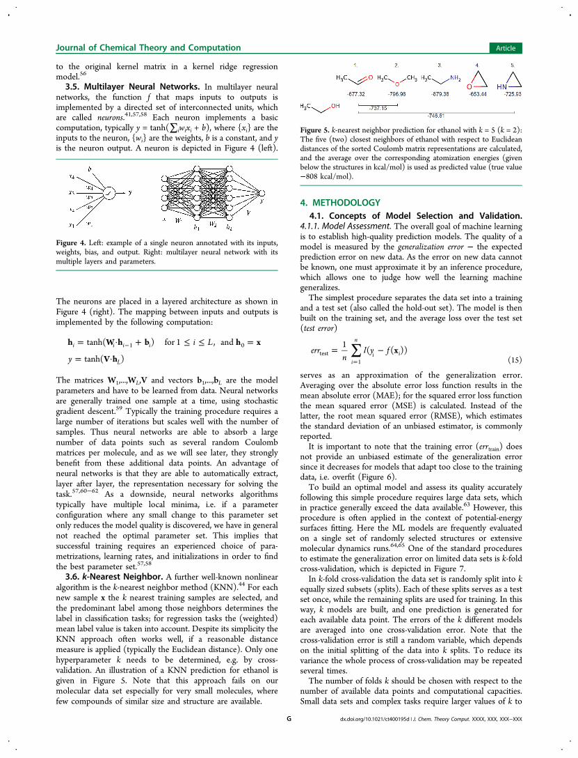
3.5. Multilayer Neural Networks. In multilayer neuralnetworks, the function f that maps inputs to outputs isimplemented by a directed set of interconnected units, whichare called neurons.41,57,58 Each neuron implements a basiccomputation, typically y = tanh(∑iwixi + b), where {xi} are theinputs to the neuron, {wi} are the weights, b is a constant, and yis the neuron output. A neuron is depicted in Figure 4 (left).

The neurons are placed in a layered architecture as shown inFigure 4 (right). The mapping between inputs and outputs isimplemented by the following computation:

= · + ≤ ≤ =

= ·− i L

y

h W h b h x

V h

tanh( ) for 1 , and

tanh( )

i i i i

L

1 0

The matrices W1,...,WL,V and vectors b1,...,bL are the modelparameters and have to be learned from data. Neural networksare generally trained one sample at a time, using stochasticgradient descent.59 Typically the training procedure requires alarge number of iterations but scales well with the number ofsamples. Thus neural networks are able to absorb a largenumber of data points such as several random Coulombmatrices per molecule, and as we will see later, they stronglybenefit from these additional data points. An advantage ofneural networks is that they are able to automatically extract,layer after layer, the representation necessary for solving thetask.57,60−62 As a downside, neural networks algorithmstypically have multiple local minima, i.e. if a parameterconfiguration where any small change to this parameter setonly reduces the model quality is discovered, we have in generalnot reached the optimal parameter set. This implies thatsuccessful training requires an experienced choice of para-metrizations, learning rates, and initializations in order to findthe best parameter set.57,58

3.6. k-Nearest Neighbor. A further well-known nonlinearalgorithm is the k-nearest neighbor method (KNN).44 For eachnew sample x the k nearest training samples are selected, andthe predominant label among those neighbors determines thelabel in classification tasks; for regression tasks the (weighted)mean label value is taken into account. Despite its simplicity theKNN approach often works well, if a reasonable distancemeasure is applied (typically the Euclidean distance). Only onehyperparameter k needs to be determined, e.g. by cross-validation. An illustration of a KNN prediction for ethanol isgiven in Figure 5. Note that this approach fails on ourmolecular data set especially for very small molecules, wherefew compounds of similar size and structure are available.

4. METHODOLOGY4.1. Concepts of Model Selection and Validation.

4.1.1. Model Assessment. The overall goal of machine learningis to establish high-quality prediction models. The quality of amodel is measured by the generalization error − the expectedprediction error on new data. As the error on new data cannotbe known, one must approximate it by an inference procedure,which allows one to judge how well the learning machinegeneralizes.The simplest procedure separates the data set into a training

and a test set (also called the hold-out set). The model is thenbuilt on the training set, and the average loss over the test set(test error)

∑= −=

errn

y f x1

( ( ))i

n

i itest1 (15)

serves as an approximation of the generalization error.Averaging over the absolute error loss function results in themean absolute error (MAE); for the squared error loss functionthe mean squared error (MSE) is calculated. Instead of thelatter, the root mean squared error (RMSE), which estimatesthe standard deviation of an unbiased estimator, is commonlyreported.It is important to note that the training error (errtrain) does

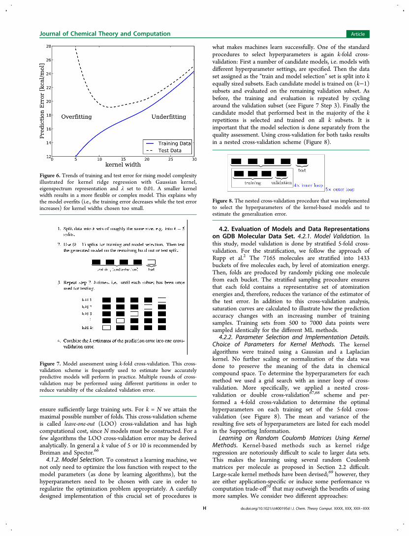
not provide an unbiased estimate of the generalization errorsince it decreases for models that adapt too close to the trainingdata, i.e. overfit (Figure 6).To build an optimal model and assess its quality accurately

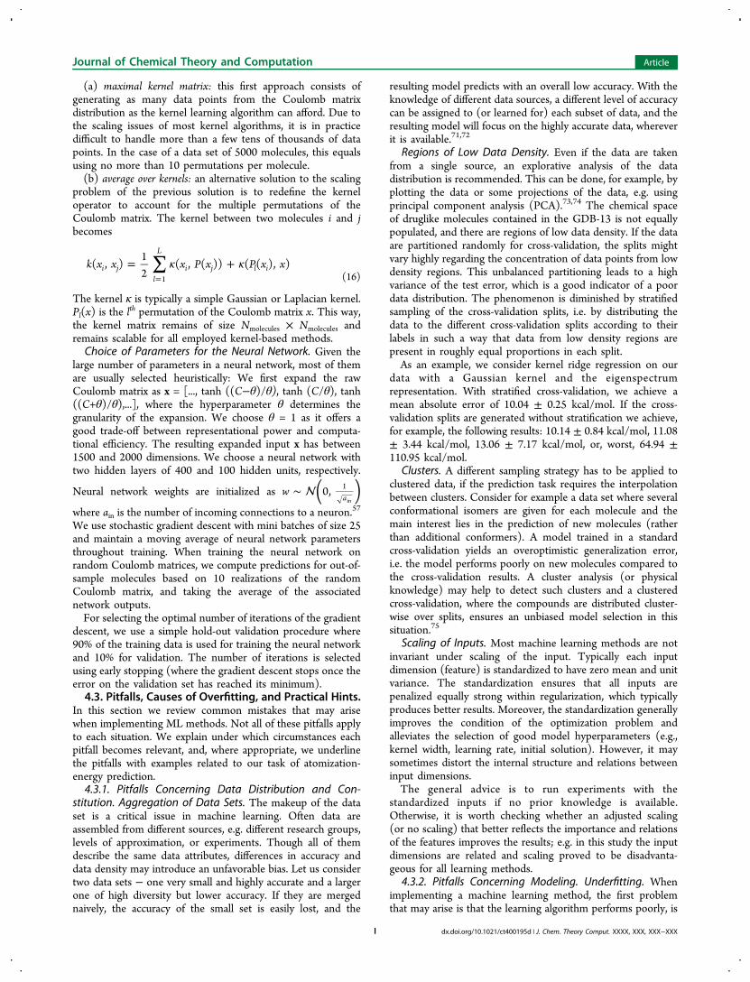
following this simple procedure requires large data sets, whichin practice generally exceed the data available.63 However, thisprocedure is often applied in the context of potential-energysurfaces fitting. Here the ML models are frequently evaluatedon a single set of randomly selected structures or extensivemolecular dynamics runs.64,65 One of the standard proceduresto estimate the generalization error on limited data sets is k-foldcross-validation, which is depicted in Figure 7.In k-fold cross-validation the data set is randomly split into k

equally sized subsets (splits). Each of these splits serves as a testset once, while the remaining splits are used for training. In thisway, k models are built, and one prediction is generated foreach available data point. The errors of the k different modelsare averaged into one cross-validation error. Note that thecross-validation error is still a random variable, which dependson the initial splitting of the data into k splits. To reduce itsvariance the whole process of cross-validation may be repeatedseveral times.The number of folds k should be chosen with respect to the

number of available data points and computational capacities.Small data sets and complex tasks require larger values of k to

Figure 4. Left: example of a single neuron annotated with its inputs,weights, bias, and output. Right: multilayer neural network with itsmultiple layers and parameters.

Figure 5. k-nearest neighbor prediction for ethanol with k = 5 (k = 2):The five (two) closest neighbors of ethanol with respect to Euclideandistances of the sorted Coulomb matrix representations are calculated,and the average over the corresponding atomization energies (givenbelow the structures in kcal/mol) is used as predicted value (true value−808 kcal/mol).

Journal of Chemical Theory and Computation Article

dx.doi.org/10.1021/ct400195d | J. Chem. Theory Comput. XXXX, XXX, XXX−XXXG

ensure sufficiently large training sets. For k = N we attain themaximal possible number of folds. This cross-validation schemeis called leave-one-out (LOO) cross-validation and has highcomputational cost, since N models must be constructed. For afew algorithms the LOO cross-validation error may be derivedanalytically. In general a k value of 5 or 10 is recommended byBreiman and Spector.66

4.1.2. Model Selection. To construct a learning machine, wenot only need to optimize the loss function with respect to themodel parameters (as done by learning algorithms), but thehyperparameters need to be chosen with care in order toregularize the optimization problem appropriately. A carefullydesigned implementation of this crucial set of procedures is

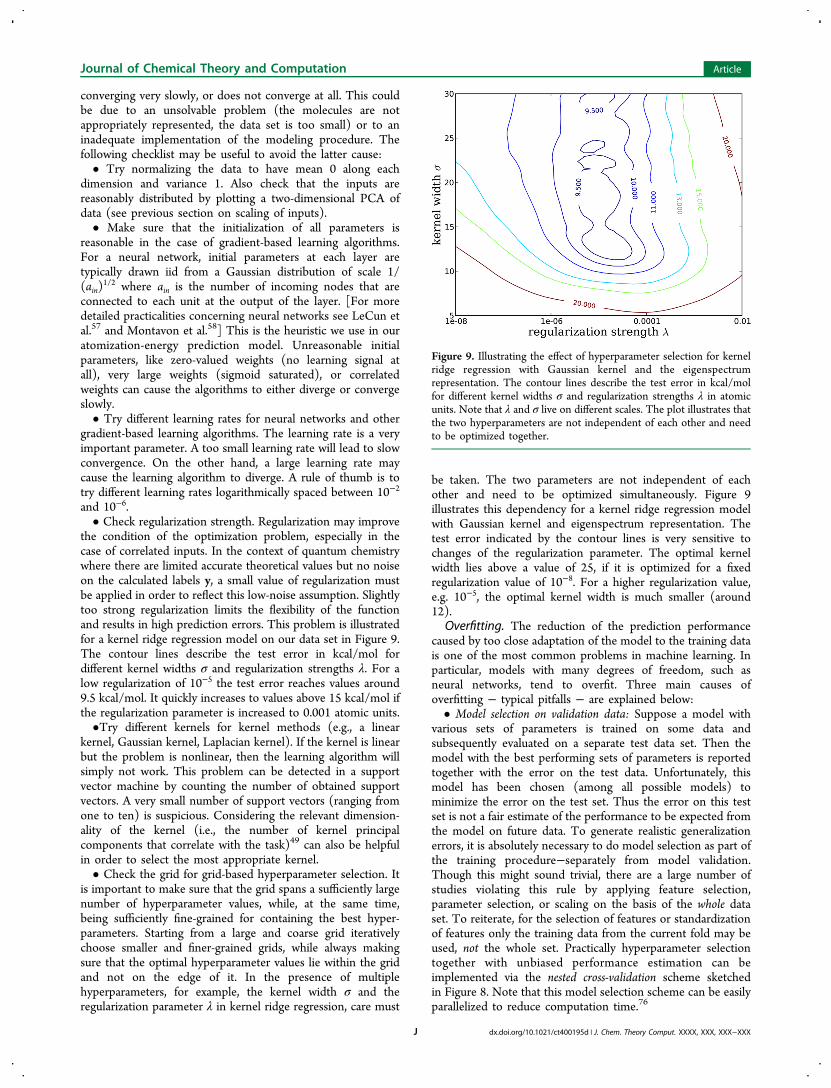
what makes machines learn successfully. One of the standardprocedures to select hyperparameters is again k-fold cross-validation: First a number of candidate models, i.e. models withdifferent hyperparameter settings, are specified. Then the dataset assigned as the “train and model selection” set is split into kequally sized subsets. Each candidate model is trained on (k−1)subsets and evaluated on the remaining validation subset. Asbefore, the training and evaluation is repeated by cyclingaround the validation subset (see Figure 7 Step 3). Finally thecandidate model that performed best in the majority of the krepetitions is selected and trained on all k subsets. It isimportant that the model selection is done separately from thequality assessment. Using cross-validation for both tasks resultsin a nested cross-validation scheme (Figure 8).

4.2. Evaluation of Models and Data Representationson GDB Molecular Data Set. 4.2.1. Model Validation. Inthis study, model validation is done by stratified 5-fold cross-validation. For the stratification, we follow the approach ofRupp et al.2 The 7165 molecules are stratified into 1433buckets of five molecules each, by level of atomization energy.Then, folds are produced by randomly picking one moleculefrom each bucket. The stratified sampling procedure ensuresthat each fold contains a representative set of atomizationenergies and, therefore, reduces the variance of the estimator ofthe test error. In addition to this cross-validation analysis,saturation curves are calculated to illustrate how the predictionaccuracy changes with an increasing number of trainingsamples. Training sets from 500 to 7000 data points weresampled identically for the different ML methods.

4.2.2. Parameter Selection and Implementation Details.Choice of Parameters for Kernel Methods. The kernelalgorithms were trained using a Gaussian and a Laplaciankernel. No further scaling or normalization of the data wasdone to preserve the meaning of the data in chemicalcompound space. To determine the hyperparameters for eachmethod we used a grid search with an inner loop of cross-validation. More specifically, we applied a nested cross-validation or double cross-validation67,68 scheme and per-formed a 4-fold cross-validation to determine the optimalhyperparameters on each training set of the 5-fold cross-validation (see Figure 8). The mean and variance of theresulting five sets of hyperparameters are listed for each modelin the Supporting Information.

Learning on Random Coulomb Matrices Using KernelMethods. Kernel-based methods such as kernel ridgeregression are notoriously difficult to scale to larger data sets.This makes the learning using several random Coulombmatrices per molecule as proposed in Section 2.2 difficult.Large-scale kernel methods have been devised;69 however, theyare either application-specific or induce some performance vscomputation trade-off70 that may outweigh the benefits of usingmore samples. We consider two different approaches:

Figure 6. Trends of training and test error for rising model complexityillustrated for kernel ridge regression with Gaussian kernel,eigenspectrum representation and λ set to 0.01. A smaller kernelwidth results in a more flexible or complex model. This explains whythe model overfits (i.e., the training error decreases while the test errorincreases) for kernel widths chosen too small.

Figure 7. Model assessment using k-fold cross-validation. This cross-validation scheme is frequently used to estimate how accuratelypredictive models will perform in practice. Multiple rounds of cross-validation may be performed using different partitions in order toreduce variability of the calculated validation error.

Figure 8. The nested cross-validation procedure that was implementedto select the hyperparameters of the kernel-based models and toestimate the generalization error.

Journal of Chemical Theory and Computation Article

dx.doi.org/10.1021/ct400195d | J. Chem. Theory Comput. XXXX, XXX, XXX−XXXH

(a) maximal kernel matrix: this first approach consists ofgenerating as many data points from the Coulomb matrixdistribution as the kernel learning algorithm can afford. Due tothe scaling issues of most kernel algorithms, it is in practicedifficult to handle more than a few tens of thousands of datapoints. In the case of a data set of 5000 molecules, this equalsusing no more than 10 permutations per molecule.(b) average over kernels: an alternative solution to the scaling

problem of the previous solution is to redefine the kerneloperator to account for the multiple permutations of theCoulomb matrix. The kernel between two molecules i and jbecomes

∑ κ κ= +=

k x x x P x P x x( , )12

( , ( )) ( ( ), )i jl

L

i j l i1 (16)

The kernel κ is typically a simple Gaussian or Laplacian kernel.Pl(x) is the l

th permutation of the Coulomb matrix x. This way,the kernel matrix remains of size Nmolecules × Nmolecules andremains scalable for all employed kernel-based methods.Choice of Parameters for the Neural Network. Given the

large number of parameters in a neural network, most of themare usually selected heuristically: We first expand the rawCoulomb matrix as x = [..., tanh ((C−θ)/θ), tanh (C/θ), tanh((C+θ)/θ),...], where the hyperparameter θ determines thegranularity of the expansion. We choose θ = 1 as it offers agood trade-off between representational power and computa-tional efficiency. The resulting expanded input x has between1500 and 2000 dimensions. We choose a neural network withtwo hidden layers of 400 and 100 hidden units, respectively.

Neural network weights are initialized as ∼ ( )w 0,a1

in

where ain is the number of incoming connections to a neuron.57

We use stochastic gradient descent with mini batches of size 25and maintain a moving average of neural network parametersthroughout training. When training the neural network onrandom Coulomb matrices, we compute predictions for out-of-sample molecules based on 10 realizations of the randomCoulomb matrix, and taking the average of the associatednetwork outputs.For selecting the optimal number of iterations of the gradient

descent, we use a simple hold-out validation procedure where90% of the training data is used for training the neural networkand 10% for validation. The number of iterations is selectedusing early stopping (where the gradient descent stops once theerror on the validation set has reached its minimum).4.3. Pitfalls, Causes of Overfitting, and Practical Hints.

In this section we review common mistakes that may arisewhen implementing ML methods. Not all of these pitfalls applyto each situation. We explain under which circumstances eachpitfall becomes relevant, and, where appropriate, we underlinethe pitfalls with examples related to our task of atomization-energy prediction.4.3.1. Pitfalls Concerning Data Distribution and Con-

stitution. Aggregation of Data Sets. The makeup of the dataset is a critical issue in machine learning. Often data areassembled from different sources, e.g. different research groups,levels of approximation, or experiments. Though all of themdescribe the same data attributes, differences in accuracy anddata density may introduce an unfavorable bias. Let us considertwo data sets − one very small and highly accurate and a largerone of high diversity but lower accuracy. If they are mergednaively, the accuracy of the small set is easily lost, and the

resulting model predicts with an overall low accuracy. With theknowledge of different data sources, a different level of accuracycan be assigned to (or learned for) each subset of data, and theresulting model will focus on the highly accurate data, whereverit is available.71,72

Regions of Low Data Density. Even if the data are takenfrom a single source, an explorative analysis of the datadistribution is recommended. This can be done, for example, byplotting the data or some projections of the data, e.g. usingprincipal component analysis (PCA).73,74 The chemical spaceof druglike molecules contained in the GDB-13 is not equallypopulated, and there are regions of low data density. If the dataare partitioned randomly for cross-validation, the splits mightvary highly regarding the concentration of data points from lowdensity regions. This unbalanced partitioning leads to a highvariance of the test error, which is a good indicator of a poordata distribution. The phenomenon is diminished by stratifiedsampling of the cross-validation splits, i.e. by distributing thedata to the different cross-validation splits according to theirlabels in such a way that data from low density regions arepresent in roughly equal proportions in each split.As an example, we consider kernel ridge regression on our

data with a Gaussian kernel and the eigenspectrumrepresentation. With stratified cross-validation, we achieve amean absolute error of 10.04 ± 0.25 kcal/mol. If the cross-validation splits are generated without stratification we achieve,for example, the following results: 10.14 ± 0.84 kcal/mol, 11.08± 3.44 kcal/mol, 13.06 ± 7.17 kcal/mol, or, worst, 64.94 ±110.95 kcal/mol.

Clusters. A different sampling strategy has to be applied toclustered data, if the prediction task requires the interpolationbetween clusters. Consider for example a data set where severalconformational isomers are given for each molecule and themain interest lies in the prediction of new molecules (ratherthan additional conformers). A model trained in a standardcross-validation yields an overoptimistic generalization error,i.e. the model performs poorly on new molecules compared tothe cross-validation results. A cluster analysis (or physicalknowledge) may help to detect such clusters and a clusteredcross-validation, where the compounds are distributed cluster-wise over splits, ensures an unbiased model selection in thissituation.75

Scaling of Inputs. Most machine learning methods are notinvariant under scaling of the input. Typically each inputdimension (feature) is standardized to have zero mean and unitvariance. The standardization ensures that all inputs arepenalized equally strong within regularization, which typicallyproduces better results. Moreover, the standardization generallyimproves the condition of the optimization problem andalleviates the selection of good model hyperparameters (e.g.,kernel width, learning rate, initial solution). However, it maysometimes distort the internal structure and relations betweeninput dimensions.The general advice is to run experiments with the

standardized inputs if no prior knowledge is available.Otherwise, it is worth checking whether an adjusted scaling(or no scaling) that better reflects the importance and relationsof the features improves the results; e.g. in this study the inputdimensions are related and scaling proved to be disadvanta-geous for all learning methods.

4.3.2. Pitfalls Concerning Modeling. Underfitting. Whenimplementing a machine learning method, the first problemthat may arise is that the learning algorithm performs poorly, is

Journal of Chemical Theory and Computation Article

dx.doi.org/10.1021/ct400195d | J. Chem. Theory Comput. XXXX, XXX, XXX−XXXI

converging very slowly, or does not converge at all. This couldbe due to an unsolvable problem (the molecules are notappropriately represented, the data set is too small) or to aninadequate implementation of the modeling procedure. Thefollowing checklist may be useful to avoid the latter cause:• Try normalizing the data to have mean 0 along each

dimension and variance 1. Also check that the inputs arereasonably distributed by plotting a two-dimensional PCA ofdata (see previous section on scaling of inputs).• Make sure that the initialization of all parameters is

reasonable in the case of gradient-based learning algorithms.For a neural network, initial parameters at each layer aretypically drawn iid from a Gaussian distribution of scale 1/(ain)

1/2 where ain is the number of incoming nodes that areconnected to each unit at the output of the layer. [For moredetailed practicalities concerning neural networks see LeCun etal.57 and Montavon et al.58] This is the heuristic we use in ouratomization-energy prediction model. Unreasonable initialparameters, like zero-valued weights (no learning signal atall), very large weights (sigmoid saturated), or correlatedweights can cause the algorithms to either diverge or convergeslowly.• Try different learning rates for neural networks and other

gradient-based learning algorithms. The learning rate is a veryimportant parameter. A too small learning rate will lead to slowconvergence. On the other hand, a large learning rate maycause the learning algorithm to diverge. A rule of thumb is totry different learning rates logarithmically spaced between 10−2

and 10−6.• Check regularization strength. Regularization may improve

the condition of the optimization problem, especially in thecase of correlated inputs. In the context of quantum chemistrywhere there are limited accurate theoretical values but no noiseon the calculated labels y, a small value of regularization mustbe applied in order to reflect this low-noise assumption. Slightlytoo strong regularization limits the flexibility of the functionand results in high prediction errors. This problem is illustratedfor a kernel ridge regression model on our data set in Figure 9.The contour lines describe the test error in kcal/mol fordifferent kernel widths σ and regularization strengths λ. For alow regularization of 10−5 the test error reaches values around9.5 kcal/mol. It quickly increases to values above 15 kcal/mol ifthe regularization parameter is increased to 0.001 atomic units.•Try different kernels for kernel methods (e.g., a linear

kernel, Gaussian kernel, Laplacian kernel). If the kernel is linearbut the problem is nonlinear, then the learning algorithm willsimply not work. This problem can be detected in a supportvector machine by counting the number of obtained supportvectors. A very small number of support vectors (ranging fromone to ten) is suspicious. Considering the relevant dimension-ality of the kernel (i.e., the number of kernel principalcomponents that correlate with the task)49 can also be helpfulin order to select the most appropriate kernel.• Check the grid for grid-based hyperparameter selection. It

is important to make sure that the grid spans a sufficiently largenumber of hyperparameter values, while, at the same time,being sufficiently fine-grained for containing the best hyper-parameters. Starting from a large and coarse grid iterativelychoose smaller and finer-grained grids, while always makingsure that the optimal hyperparameter values lie within the gridand not on the edge of it. In the presence of multiplehyperparameters, for example, the kernel width σ and theregularization parameter λ in kernel ridge regression, care must

be taken. The two parameters are not independent of eachother and need to be optimized simultaneously. Figure 9illustrates this dependency for a kernel ridge regression modelwith Gaussian kernel and eigenspectrum representation. Thetest error indicated by the contour lines is very sensitive tochanges of the regularization parameter. The optimal kernelwidth lies above a value of 25, if it is optimized for a fixedregularization value of 10−8. For a higher regularization value,e.g. 10−5, the optimal kernel width is much smaller (around12).

Overfitting. The reduction of the prediction performancecaused by too close adaptation of the model to the training datais one of the most common problems in machine learning. Inparticular, models with many degrees of freedom, such asneural networks, tend to overfit. Three main causes ofoverfitting − typical pitfalls − are explained below:• Model selection on validation data: Suppose a model with

various sets of parameters is trained on some data andsubsequently evaluated on a separate test data set. Then themodel with the best performing sets of parameters is reportedtogether with the error on the test data. Unfortunately, thismodel has been chosen (among all possible models) tominimize the error on the test set. Thus the error on this testset is not a fair estimate of the performance to be expected fromthe model on future data. To generate realistic generalizationerrors, it is absolutely necessary to do model selection as part ofthe training procedure−separately from model validation.Though this might sound trivial, there are a large number ofstudies violating this rule by applying feature selection,parameter selection, or scaling on the basis of the whole dataset. To reiterate, for the selection of features or standardizationof features only the training data from the current fold may beused, not the whole set. Practically hyperparameter selectiontogether with unbiased performance estimation can beimplemented via the nested cross-validation scheme sketchedin Figure 8. Note that this model selection scheme can be easilyparallelized to reduce computation time.76

Figure 9. Illustrating the effect of hyperparameter selection for kernelridge regression with Gaussian kernel and the eigenspectrumrepresentation. The contour lines describe the test error in kcal/molfor different kernel widths σ and regularization strengths λ in atomicunits. Note that λ and σ live on different scales. The plot illustrates thatthe two hyperparameters are not independent of each other and needto be optimized together.

Journal of Chemical Theory and Computation Article

dx.doi.org/10.1021/ct400195d | J. Chem. Theory Comput. XXXX, XXX, XXX−XXXJ

• Hyperparameters: Like with underfitting, inappropriateselection of hyperparameters, especially the regularizationstrength, may cause overfitting. As an example Figure 6illustrates how an unfavorable selection of the kernel width σcan cause overfitting of a kernel ridge regression model on ourdata.• Neglect of baselines: Overfitting is also defined as the

violation of Occam’s Razor by using a more complicated modelthan necessary.77 If a complex model is directly applied withoutconsidering simple models, then the solution found may bemore complex than the underlying problem and more intuitiverelations between input and output data will remainundetected. Thus, it is desirable to additionally report resultson simple baseline models like, the mean predictor, linearregression, or KNN in order to determine the need for complexmodels.

5. RESULTS AND DISCUSSION

Here, we apply the techniques described in the first part of thepaper (learning algorithms, data representations, and method-ology) to the problem of predicting atomization energies fromraw molecular geometries. We run extensive simulations on acluster of CPUs and compare the performance in terms ofcross-validation error of the learning algorithms shown inSection 3 and data representations described in Section 2. We

also discuss computational aspects such as training time,prediction speed, and scalability of these algorithms with thenumber of samples.

Cross-Validation Study. The cross-validation results foreach learning algorithm and representation are listed in Table 3.The algorithms are grouped into five categories: basic machinelearning methods which serve as baselines, kernel methodsusing a Gaussian kernel, kernel methods using a Laplaciankernel, neural networks, and two physically motivatedapproaches reported by Moussa.35

We first observe that ML baseline models in the first categoryare clearly off-the-mark compared to the other moresophisticated ML models such as kernel methods andmultilayer neural networks. This shows that the problem ofpredicting first-principles molecular energetics is a complexone. Among the set of baseline methods, linear regressionperforms significantly better (best MAE 20.72 kcal/mol) thank-nearest neighbors on this data set (best MAE 70.72 kcal/mol). This indicates that there are meaningful linear relationsbetween physical quantities in the system and that it isinsufficient to simply look up the most similar molecules (as k-nearest neighbors does). The k-nearest neighbors approach failsto create a smooth mapping to the energies.Next, the kernel methods with Gaussian kernel are compared

to the methods that use the Laplacian kernel (instead of the

Table 3. Prediction Errors (In Terms of Mean Absolute Error and Root Mean Squared Error ± Standard Deviation) for SeveralAlgorithms and Representationsa

algorithm molecule representation MAE [kcal/mol] RMSE [kcal/mol]

basic methods mean predictor none 179.02 ± 0.08 223.92 ± 0.32k-nearest neighbors eigenspectrum 70.72 ± 2.12 92.49 ± 2.70

sorted Coulomb 71.54 ± 0.97 95.97 ± 1.45linear regression eigenspectrum 29.17 ± 0.35 38.01 ± 1.11

sorted Coulomb 20.72 ± 0.32 27.22 ± 0.84methods with Gaussian kernel mixed effects eigenspectrum 10.50 ± 0.48 20.38 ± 9.29

sorted Coulomb 8.5 ± 0.45 12.16 ± 0.95kernel support eigenspectrum 10.78 ± 0.58 19.47 ± 9.46vector regression sorted Coulomb 8.06 ± 0.38 12.59 ± 2.17kernel ridge regression eigenspectrum 10.04 ± 0.25 17.02 ± 2.51

sorted Coulomb 8.57 ± 0.40 12.26 ± 0.78random Coulomb (2) 8.46 ± 0.21 11.99 ± 0.73random Coulomb (5) 7.10 ± 0.22 10.43 ± 0.83random Coulomb (8) 6.76 ± 0.21 10.09 ± 0.76average random Coulomb (250) 7.79 ± 0.42 11.40 ± 1.11

methods with Laplacian kernel mixed effects eigenspectrum 9.79 ± 0.37 13.18 ± 0.79sorted Coulomb 4.29 ± 0.12 6.51 ± 0.56

kernel support eigenspectrum 9.46 ± 0.39 13.26 ± 0.85vector regression sorted Coulomb 3.99 ± 0.16 6.45 ± 0.71kernel ridge regression eigenspectrum 9.96 ± 0.25 13.29 ± 0.59

sorted Coulomb 4.28 ± 0.11 6.47 ± 0.51random Coulomb (2) 4.02 ± 0.07 5.98 ± 0.35random Coulomb (5) 3.29 ± 0.08 5.10 ± 0.39random Coulomb (8) 3.07 ± 0.07 4.84 ± 0.40average random Coulomb (250) 4.10 ± 0.14 6.16 ± 0.65

multilayer neural network backpropagation eigenspectrum 14.08 ± 0.29 20.29 ± 0.73sorted Coulomb 11.82 ± 0.45 16.01 ± 0.81random Coulomb (1000) 3.51 ± 0.13 5.96 ± 0.48

previous PM6 atoms and coordinates 4.9 6.3bond counting covalent bonds 10.0 13.0

aThe ML algorithms are grouped into four categories: basic machine learning methods which serve as baselines, kernel methods using Gaussiankernel, kernel methods using Laplacian kernel, and neural networks. For comparison results for bond counting and PM6 (adjusted to this data set) asreported by Moussa35 are given. (Some of the ML results are also included in a preliminary conference contribution.37)

Journal of Chemical Theory and Computation Article

dx.doi.org/10.1021/ct400195d | J. Chem. Theory Comput. XXXX, XXX, XXX−XXXK

Gaussian). The Laplacian kernel seems to be better suited forthe prediction problem than the Gaussian kernel, as it improvesresults for all kernel methods. In order to gain insight into thekernel functions we compare the effect of the Manhattandistance metric and the Euclidean distance metric on thedistribution of distances between molecules in Figure 10. (Notethat the main difference between Laplacian and Gaussian kernelis the use of the Manhattan distance instead of the Euclideandistance.) The Euclidean distances lie in two narrow separategroups, while the Manhattan distance spreads a much largerrange of distances and shows larger variety with respect todifferent stoichiometries of the molecules. One might speculatethat the Laplacian kernel with its Manhattan distance metricbetter encodes the approximately additive nature of atomizationenergy than the Gaussian kernel with its Euclidean distancemetric. Additionally, the longer tails of the Laplacian kernel andits nondifferentiable peak at the center help to model piecewise-

smooth functions (i.e., composed of cliffs and linear plateaus).Such piecewise smoothness may arise as a result of the highlycomplex nature of the learning problem or possibly due tosuboptimal molecular representations.The results on all ML methods illustrate the impact of the

molecule representation on the prediction performance. Forkernel ridge regression with Laplacian kernel the trend is themost distinct: the random Coulomb matrix representationperforms best (MAE down to 3.07 kcal/mol), followed by thesorted Coulomb matrix (MAE 4.28 kcal/mol) and theeigenspectrum (MAE 9.96 kcal/mol). This ordering correlateswith the amount of information provided by the differentrepresentations: The randomly sorted Coulomb matrixrepresentation is the richest one as it is both high-dimensionaland accounting for multiple indexing of atoms. This is bestillustrated in Figure 11 where Coulomb matrix realizations form“clouds” of data points with a particular size, orientation, or

Figure 10. Distribution of pairwise distances within the GDB data set based on the sorted Coulomb representation of molecules (in hartree). Theleft plot illustrates the distribution of Euclidean distances between molecules. The cluster between 320 and 410 consists of distances betweenmolecules with different number of sulfur atoms. The other cluster includes pairs of molecules having both none or both one sulfur atom. For theManhattan distance metric (right plot) these clusters are less pronounced, and the distance values show a much larger variety. This may aid theprediction task.

Figure 11. Two-dimensional PCA of the distribution of random Coulomb matrices illustrated for 50 molecules (calculated over the set of allmolecules). The Manhattan distance between Coulomb matrices is given as input to PCA. Each cloud of same-colored points represents onemolecule, and each point within a cloud designates one random Coulomb matrix associated with the molecule.

Journal of Chemical Theory and Computation Article

dx.doi.org/10.1021/ct400195d | J. Chem. Theory Comput. XXXX, XXX, XXX−XXXL

shape for each molecule. This cloud-related information ismissing in the sorted Coulomb matrix representation, as eachmolecule is represented by only one data point. Theeigenspectrum representation has the lowest performance inour study, in part, because different Coulomb matrices mayresult in the same eigenspectrum and information is lost in thismapping. This reduction of information has a particularlydramatic impact on the performance of complex models (e.g.,kernel ridge regression or neural networks), as they are nolonger able to exploit the wealth of information available in theprevious representations.The last group of ML method presents results for multilayer

neural networks. Interestingly, these methods do not performbetter than kernel methods on the eigenspectrum representa-tion (neural networks MAE 14.08 kcal/mol, while kernelmethods are below 10.5 kcal/mol). Moving from theeigenspectrum to the sorted Coulomb matrices neural networksimprove significantly (MAE 11.82 kcal/mol), and finally neuralnetworks are almost on par with the kernel methodsconsidering the random Coulomb matrix representation.Note that using many randomly permuted Coulomb matrices(typically more than 1000 per molecule) is crucial for obtaininggood performance in the order of MAE 3.5 kcal/mol with aneural network (while for kernel ridge regression models fivepermutations are sufficient). Figure 11 shows how randompermutations of the Coulomb matrix help to fill the input spacewith data points and, thus, allow for learning complex, yetstatistically significant decision boundaries.

The last category includes results on bond counting and thesemiempirical method PM63 taken from Moussa.35 Bondenergies are refit to the given data set, and PM6 is converted toan electronic energy using a per-atom correction in order toallow for a fair comparison to data driven ML methods. Hisvalidation setup slightly deviates from our study (static trainingset of 5000 compounds instead of 5-fold cross-validation). Thismay introduce a bias in the MAE. However, this will not affectthe qualitative results: simple ML models are clearly inferior tobond counting or PM6 methods that have been adjusted to thedata set. However, bond counting uses explicit informationabout covalent bond orders. This information is not explicitlyincluded in the Coulomb matrix. Given that, it is important tonote that the best kernel ridge regression model achieves aMAE of 3.1 kcal/mol compared to 4.9 kcal/mol (PM6) and10.0 kcal/mol (bond counting).

Saturation Study. The results of the saturation study aresummarized in Figure 12. The learning curves (cf. ref 78)illustrate the power-law decline of the prediction error withincreasing amount of training data. Each curve can becharacterized by the initial error and the “learning rate”, i.e.the slope of the learning curve in the log−log plot. The curvesfor the mean predictor and the KNN model are rather flat,indicating low learning capacity. The steepest learning curve isobtained by the neural network based on 1000 randomlypermuted Coulomb matrices per molecule. This may beattributed to the fact that the neural network gradually learnsthe data representation (in its multiple layers) as more data

Figure 12. Saturation curves for various ML models and representations (KRR = kernel ridge regression, NN = multilayer neural network, Mean =mean predictor, KNN = k-nearest neighbors, laplace = with Laplacian kernel, gauss = with Gaussian kernel, sorted = using sorted Coulombrepresentation, 2/5/8/1000 = using 2/5/8/1000 random Coulomb matrices to represent one molecule). Left: Log−log plot where the slope of theline reflects the learning rate of the algorithm. Right: nonlogarithmic learning curves for kernel ridge regression and neural network models. Kernelridge regression with Laplacian kernel and 8 random Coulomb matrices per molecule performs best. However, due to the scaling problem of kernelmethods, the representation of 8 random Coulomb matrices per molecule could not be used with kernel ridge regression for data sets larger than5500 molecules.

Journal of Chemical Theory and Computation Article

dx.doi.org/10.1021/ct400195d | J. Chem. Theory Comput. XXXX, XXX, XXX−XXXM

become available. The neural networks still do not performbetter than the kernel ridge regression model with eightrandomly permuted Coulomb matrices and a Laplacian kernel.The latter already yields good results on smaller data sets anddemonstrates the gain of providing the learning algorithm witha good similarity measure (or kernel). However, for therepresentation of eight random Coulomb matrices per moleculethe learning curve of kernel methods is incomplete. Thecalculation failed for more than 5500 molecules (i.e., a kernelmatrix of (5500·8)2 = 1936 × 106 entries). These scalingproblems together with calculation times are discussed in thenext section. In summary, the saturation study confirms ourprevious observations: The baseline methods cannot competewith sophisticated ML algorithms, the Laplacian kernel yieldsbetter results than the Gaussian kernel, and among the threedifferent molecular representations the random Coulombmatrices perform best.The saturation study also illustrates the limits of the

presented approaches: The molecular representation andapplied algorithm define the maximal reachable accuracy.Even large data sets can barely improve the performance ofthe best models below 3 kcal/mol. Note that the accuracy ofour energy calculation is estimated to be on the order of 3 kcal/mol. Even a perfect model that reflects chemical reality wouldprobably yield errors in this order of magnitude. Only a moreaccurate or larger data set could clarify which furtherenhancements of the algorithms and chemical representationsare recommendable in order to explore chemical compoundspace.Runtime Comparison. Training and prediction times of

most ML methods depend on the size n of the training set andthe maximal size of a molecule or more precisely thedimensionality of the vector representing each molecule d.Runtime obviously depends on the machine as well as theimplementation used. For this reason, the numbers given hereare only meant to provide generic guidance.In general, baseline methods, e.g. the k-nearest neighbors or

linear regression, are fast to train. The k-nearest neighborsapproach does not require any training and takes less than 1 sto predict 1000 compounds using either a sorted Coulomb oreigenspectrum representation. However, the prediction time ofk-nearest neighbors scales with the number of training samples( (n)), while the prediction time of linear regression isindependent of n. (It only scales with the dimensionality d ofthe input.)Kernel ridge regression as well as mixed effects models take

only a few seconds to train on 3000 samples using theeigenspectrum or sorted Coulomb representation for one set ofhyperparameters. However, training times for mixed effectsmodels as well as kernel ridge regression models scale with(n3) and require (n2) memory space. Prediction on our data

set is fast (less than 1 s for 1000 samples) but scales linearlywith n. Kernel ridge regression with 3000 training samples on astochastic Coulomb representation with eight permutations stilltakes only a matter of minutes.Support vector regression is implemented using an iterative

approach. When a fixed number of iterations is assumed,support vector regression training and testing scale with (n·nsv+ nsv

3 ) and (nsv), respectively, where nsv is the number ofsupport vectors. For 3000 training samples, support vectorregression training times varied from a few seconds to about 1 hdepending on the cost parameter and representation.Prediction is fast and takes less than 1 s for 1000 samples. In

general, support vector regression trades training speed forprediction speed as the learning algorithm seeks to minimizethe number of data points that contribute to the predictionfunction.For kernel methods the influence of the input dimensionality

d on the runtime depends on the used kernel. Generallycomputation times of kernels grow slowly with risingdimensionality which makes kernel methods a favorable toolfor small high-dimensional data sets.The only algorithm that requires more than a few minutes for

training is the multilayer neural network, which took about 15min to train on 3000 compounds using the sorted Coulombrepresentation and about 10 h to train on the stochasticCoulomb representation with 1000 permutations. While this isslow compared with the other methods, the multilayer neuralnetwork offers the advantage of (almost) linear scaling in(kn) for training, where k is the size of the network, which

grows with n and d. Unlike training, prediction in a neuralnetwork is fast (less than 1 s for 1000 samples) and does onlydepend on the size of the network.

6. CONCLUSIONSAlgorithms that can predict energies of ground-state moleculesquickly and accurately are a powerful tool and might contributesubstantially to rational compound design in chemical andpharmaceutical industries. However, state-of-the-art ab initiocalculations that achieve the “chemical accuracy” of 1 kcal/molare typically subject to prohibitive computational costs. Thismakes the understanding of complex chemical systems a hardtask and the exploration of chemical compound spaceunfeasible. Semiempirical models on the other side tradeaccuracy for speed. Here machine learning can provide aninteresting contribution barely compromising in this trade-off.Specifically, we show that machine learning allows one todrastically accelerate the computation of quantum-chemicalproperties, while retaining high prediction accuracy.All ML algorithms surveyed in this work achieve the first goal

of making quantum-chemical computation a matter ofmilliseconds rather than hours or days when using ab initiocalculations.With respect to prediction accuracy, our results improve over

the 10 kcal/mol MAE using kernel ridge regression that wasreported recently by Rupp et al.2 While simple baseline MLmethods such as linear regression and k-nearest neighbors arenot suited for this task, more sophisticated methods such askernel-based learning methods or neural networks yieldprediction errors as low as 3 kcal/mol achieved out-of-sample.This substantial improvement results from a combination ofmultiple factors such as a choice of model (such as the kernelfunction) and an appropriate representation of the physicalproperties and invariance structure of molecules (randomCoulomb matrices). These factors interact in a complexmanner; our analysis is a first step and further investigationshould follow.The focus of this work was on the prediction of ground-state

atomization energies for small molecules. However, all methodsalso provide derivatives which can be used as forces in atomisticsimulations. Whether these forces are (given an appropriatetraining set) of similar accuracy as the predicted atomizationenergies is a point of further research.24 Moreover, alternativerepresentations of molecules should be elaborated for thisdifferent task−especially when moving to large systems likeproteins.

Journal of Chemical Theory and Computation Article

dx.doi.org/10.1021/ct400195d | J. Chem. Theory Comput. XXXX, XXX, XXX−XXXN

One practical contribution of this work was to establish abest-practice use of ML methods. Having done this we clearlypoint to erroneous modeling and model selection (which isunfortunately still quite common in applications of MLmethods). We reiterate the fact that ML techniques can beerror prone if the modeling does not adhere to a strictmethodology, in particular, training and validation procedures.Failing to select hyperparameters appropriately or to keep testdata aside will likely lead to overly optimistic assessment of themodel’s generalization capabilities.Modeling and model assessment are always limited to the

available data regime; thus predictions beyond the spacesampled by the training data carry uncertainty. For futurestudies it will be important to further explore, understand, andquantify these limits as well as to enlarge the investigatedcompound space. Many ML methods are not designed toextrapolate. However, their interpolation in a nonlinearlytransformed space is much different from common linearinterpolations in the data space (see Figure 3).There is no learning algorithm that works optimally on all

data sets. Generally, we recommend a bottom-up approach,starting from simple (linear) baseline algorithms and thengradually increasing the complexity of the ML method forfurther improving model accuracy.Concluding, ML methods implement a powerful, fast, and

unbiased approach to the task of energy prediction in the sensethat they neither build on specific physical knowledge nor arethey limited by physical assumptions or approximations. Futurestudies will focus on methods to decode the trained nonlinearML models in order to obtain a deeper physical understandingand new insights into complex chemical systems.

■ ASSOCIATED CONTENT*S Supporting InformationThe data set and the used splits plus a Python packageincluding the scripts to run one of the used algorithms can befound at http://quantum-machine.org/. A table summarizingthe parameters selected for each method in cross-validation.This material is available free of charge via the Internet athttp://pubs.acs.org.

■ AUTHOR INFORMATIONCorresponding Author*E-mail: hansen@fhi-berlin.mpg.de (K.H.), klaus-robert.mueller@tu-berlin.de (K.R.M.).NotesThe authors declare no competing financial interest.

■ ACKNOWLEDGMENTSThis work is supported by the European Research Council(ERC Starting Grant VDW-CMAT), by the World ClassUniversity Program through the National Research Foundationof Korea funded by the Ministry of Education, Science, andTechnology, under Grant R31-10008, the Einstein Foundation,and by the U.S. Department of Energy, Basic Energy Sciences,Office of Science, under contract # DE-AC02-06CH11357. Thework of Franziska Biegler is funded, in part, by the NaturalSciences and Engineering Research Council of Canada. Theauthors also acknowledge partial support by DFG (MU 987/17-1). Matthias Rupp acknowledges support by FP7 pro-gramme of the European Community (Marie Curie IEF273039).

■ REFERENCES(1) Montavon, G.; Rupp, M.; Gobre, V.; Vazquez-Mayagoitia, A.;Hansen, K.; Tkatchenko, A.; Muller, K.-R.; von Lilienfeld, O. A. New J.Phys. 2013, accepted.(2) Rupp, M.; Tkatchenko, A.; Muller, K.-R.; von Lilienfeld, O. A.Phys. Rev. Lett. 2012, 108, 058301.(3) Stewart, J. J. P. J. Mol. Model. 2007, 13, 1173−1213.(4) Benson, S. W. Bond energies; 1965. http://www.wiredchemist.com (accessed June 8, 2011).(5) Behler, J. Phys. Chem. Chem. Phys. 2011, 13, 17930−17955.(6) Breiman, L. Stat. Sci. 2001, 16, 199−231 Mathematical Reviewsnumber (MathSciNet): MR1874152.(7) Montavon, G.; Braun, M. L.; Krueger, T.; Muller, K.-R. SignalProcessing Magazine, IEEE 2013, 30, 62−74.(8) Selassie, C. The History of Quantitative Structure ActivityRelationships. In Burger’s Medicinal Chemistry and Drug Discovery, 6thed.; Abraham, D., Ed.; John Wiley and Sons Publishers: New York,NY, 2003; Vol. 1, Chapter 1, pp 1−48.(9) Muller, K.-R.; Ratsch, G.; Mika, S.; Sonnenburg, S.; Grimm, M.;Heinrich, N. J. Chem. Inf. Model. 2005, 45, 249−253.(10) Le Bailly de Tilleghem, C.; Govaerts, B. A review of quantitativestructure-activity relationship (QSAR) models; Technical Report 07027;Universite catholique de Louvain, 2007.(11) Sumpter, B. G.; Noid, D. W. Chem. Phys. Lett. 1992, 192, 455−462.(12) Blank, T. B.; Brown, S. D.; Calhoun, A. W.; Doren, D. J. J. Chem.Phys. 1995, 103, 4129.(13) Lorenz, S.; Groß, A.; Scheffler, M. Chem. Phys. Lett. 2004, 395,210−215.(14) Lorenz, S.; Scheffler, M.; Gross, A. Phys. Rev. B 2006, 73,115431.(15) Manzhos, S.; Carrington, T. J. Chem. Phys. 2006, 125, 084109.(16) Hu, L.; Wang, X.; Wong, L.; Chen, G. J. Chem. Phys. 2003, 119,11501.(17) Zheng, X.; Hu, L.; Wang, X.; Chen, G. Chem. Phys. Lett. 2004,390, 186−192.(18) Behler, J.; Parrinello, M. Phys. Rev. Lett. 2007, 98, 146401.(19) Handley, C. M.; Popelier, P. L. A. J. Chem. Theory Comput.2009, 5, 1474−1489.(20) Behler, J.; Martonak, R.; Donadio, D.; Parrinello, M. Phys. Rev.Lett. 2008, 100, 185501.(21) Mills, M. J.; Popelier, P. L. Comput. Theor. Chem. 2011, 975,42−51.(22) Bartok, A. P.; Payne, M. C.; Kondor, R.; Csanyi, G. Phys. Rev.Lett. 2010, 104, 136403.(23) Pozun, Z. D.; Hansen, K.; Sheppard, D.; Rupp, M.; Muller, K.-R.; Henkelman, G. J. Chem. Phys. 2012, 136, 174101.(24) Snyder, J. C.; Rupp, M.; Hansen, K.; Muller, K.-R.; Burke, K.Phys. Rev. Lett. 2012, 108, 253002.(25) Hautier, G.; Fisher, C. C.; Jain, A.; Mueller, T.; Ceder, G. Chem.Mater. 2010, 22, 3762−3767.(26) Balabin, R. M.; Lomakina, E. I. J. Chem. Phys. 2009, 131,074104.(27) Balabin, R. M.; Lomakina, E. I. Phys. Chem. Chem. Phys. 2011,13, 11710−11718.(28) Blum, L. C.; Reymond, J.-L. J. Am. Chem. Soc. 2009, 131, 8732−8733.(29) Weininger, D. J. Chem. Inf. Model. 1988, 28, 31−36.(30) Guha, R.; Howard, M. T.; Hutchison, G. R.; Murray-Rust, P.;Rzepa, H.; Steinbeck, C.; Wegner, J.; Willighagen, E. L. J. Chem. Inf.Model. 2006, 46, 991−998.(31) Rappe, A. K.; Casewit, C. J.; Colwell, K. S.; Goddard, W. A.;Skiff, W. M. J. Am. Chem. Soc. 1992, 114, 10024−10035.(32) Perdew, J. P.; Burke, K.; Ernzerhof, M. Phys. Rev. Lett. 1996, 77,3865.(33) Ernzerhof, M.; Scuseria, G. E. J. Chem. Phys. 1999, 110, 5029−5036.(34) Blum, V.; Gehrke, R.; Hanke, F.; Havu, P.; Havu, V.; Ren, X.;Reuter, K.; Scheffler, M. Comput. Phys. Commun. 2009, 180, 2175.

Journal of Chemical Theory and Computation Article

dx.doi.org/10.1021/ct400195d | J. Chem. Theory Comput. XXXX, XXX, XXX−XXXO

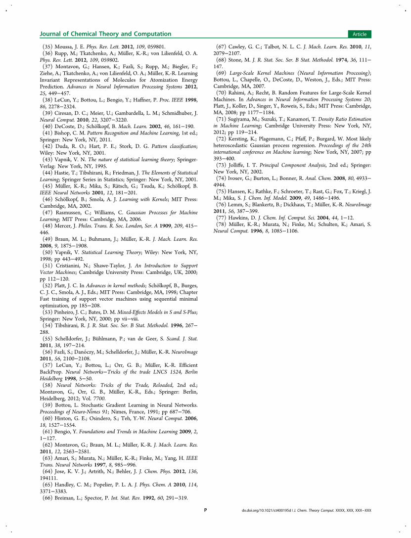
(35) Moussa, J. E. Phys. Rev. Lett. 2012, 109, 059801.(36) Rupp, M.; Tkatchenko, A.; Muller, K.-R.; von Lilienfeld, O. A.Phys. Rev. Lett. 2012, 109, 059802.(37) Montavon, G.; Hansen, K.; Fazli, S.; Rupp, M.; Biegler, F.;Ziehe, A.; Tkatchenko, A.; von Lilienfeld, O. A.; Muller, K.-R. LearningInvariant Representations of Molecules for Atomization EnergyPrediction. Advances in Neural Information Processing Systems 2012,25, 449−457.(38) LeCun, Y.; Bottou, L.; Bengio, Y.; Haffner, P. Proc. IEEE 1998,86, 2278−2324.(39) Ciresan, D. C.; Meier, U.; Gambardella, L. M.; Schmidhuber, J.Neural Comput. 2010, 22, 3207−3220.(40) DeCoste, D.; Scholkopf, B. Mach. Learn. 2002, 46, 161−190.(41) Bishop, C. M. Pattern Recognition and Machine Learning, 1st ed.;Springer: New York, NY, 2011.(42) Duda, R. O.; Hart, P. E.; Stork, D. G. Pattern classification;Wiley: New York, NY, 2001.(43) Vapnik, V. N. The nature of statistical learning theory; Springer-Verlag: New York, NY, 1995.(44) Hastie, T.; Tibshirani, R.; Friedman, J. The Elements of StatisticalLearning; Springer Series in Statistics; Springer: New York, NY, 2001.(45) Muller, K.-R.; Mika, S.; Ratsch, G.; Tsuda, K.; Scholkopf, B.IEEE Neural Networks 2001, 12, 181−201.(46) Scholkopf, B.; Smola, A. J. Learning with Kernels; MIT Press:Cambridge, MA, 2002.(47) Rasmussen, C.; Williams, C. Gaussian Processes for MachineLearning; MIT Press: Cambridge, MA, 2006.(48) Mercer, J. Philos. Trans. R. Soc. London, Ser. A 1909, 209, 415−446.(49) Braun, M. L.; Buhmann, J.; Muller, K.-R. J. Mach. Learn. Res.2008, 9, 1875−1908.(50) Vapnik, V. Statistical Learning Theory; Wiley: New York, NY,1998; pp 443−492.(51) Cristianini, N.; Shawe-Taylor, J. An Introduction to SupportVector Machines; Cambridge University Press: Cambridge, UK, 2000;pp 112−120.(52) Platt, J. C. In Advances in kernel methods; Scholkopf, B., Burges,C. J. C., Smola, A. J., Eds.; MIT Press: Cambridge, MA, 1998; ChapterFast training of support vector machines using sequential minimaloptimization, pp 185−208.(53) Pinheiro, J. C.; Bates, D. M. Mixed-Effects Models in S and S-Plus;Springer: New York, NY, 2000; pp vii−viii.(54) Tibshirani, R. J. R. Stat. Soc. Ser. B Stat. Methodol. 1996, 267−288.(55) Schelldorfer, J.; Buhlmann, P.; van de Geer, S. Scand. J. Stat.2011, 38, 197−214.(56) Fazli, S.; Danoczy, M.; Schelldorfer, J.; Muller, K.-R. NeuroImage2011, 56, 2100−2108.(57) LeCun, Y.; Bottou, L.; Orr, G. B.; Muller, K.-R. EfficientBackProp. Neural Networks−Tricks of the trade LNCS 1524, BerlinHeidelberg 1998, 5−50.(58) Neural Networks: Tricks of the Trade, Reloaded, 2nd ed.;Montavon, G., Orr, G. B., Muller, K.-R., Eds.; Springer: Berlin,Heidelberg, 2012; Vol. 7700.(59) Bottou, L. Stochastic Gradient Learning in Neural Networks.Proceedings of Neuro-Nimes 91; Nimes, France, 1991; pp 687−706.(60) Hinton, G. E.; Osindero, S.; Teh, Y.-W. Neural Comput. 2006,18, 1527−1554.(61) Bengio, Y. Foundations and Trends in Machine Learning 2009, 2,1−127.(62) Montavon, G.; Braun, M. L.; Muller, K.-R. J. Mach. Learn. Res.2011, 12, 2563−2581.(63) Amari, S.; Murata, N.; Muller, K.-R.; Finke, M.; Yang, H. IEEETrans. Neural Networks 1997, 8, 985−996.(64) Jose, K. V. J.; Artrith, N.; Behler, J. J. Chem. Phys. 2012, 136,194111.(65) Handley, C. M.; Popelier, P. L. A. J. Phys. Chem. A 2010, 114,3371−3383.(66) Breiman, L.; Spector, P. Int. Stat. Rev. 1992, 60, 291−319.

(67) Cawley, G. C.; Talbot, N. L. C. J. Mach. Learn. Res. 2010, 11,2079−2107.(68) Stone, M. J. R. Stat. Soc. Ser. B Stat. Methodol. 1974, 36, 111−147.(69) Large-Scale Kernel Machines (Neural Information Processing);Bottou, L., Chapelle, O., DeCoste, D., Weston, J., Eds.; MIT Press:Cambridge, MA, 2007.(70) Rahimi, A.; Recht, B. Random Features for Large-Scale KernelMachines. In Advances in Neural Information Processing Systems 20;Platt, J., Koller, D., Singer, Y., Roweis, S., Eds.; MIT Press: Cambridge,MA, 2008; pp 1177−1184.(71) Sugiyama, M.; Suzuki, T.; Kanamori, T. Density Ratio Estimationin Machine Learning; Cambridge University Press: New York, NY,2012; pp 119−214.(72) Kersting, K.; Plagemann, C.; Pfaff, P.; Burgard, W. Most likelyheteroscedastic Gaussian process regression. Proceedings of the 24thinternational conference on Machine learning; New York, NY, 2007; pp393−400.(73) Jolliffe, I. T. Principal Component Analysis, 2nd ed.; Springer:New York, NY, 2002.(74) Ivosev, G.; Burton, L.; Bonner, R. Anal. Chem. 2008, 80, 4933−4944.(75) Hansen, K.; Rathke, F.; Schroeter, T.; Rast, G.; Fox, T.; Kriegl, J.M.; Mika, S. J. Chem. Inf. Model. 2009, 49, 1486−1496.(76) Lemm, S.; Blankertz, B.; Dickhaus, T.; Muller, K.-R. NeuroImage2011, 56, 387−399.(77) Hawkins, D. J. Chem. Inf. Comput. Sci. 2004, 44, 1−12.(78) Muller, K.-R.; Murata, N.; Finke, M.; Schulten, K.; Amari, S.Neural Comput. 1996, 8, 1085−1106.

Journal of Chemical Theory and Computation Article

dx.doi.org/10.1021/ct400195d | J. Chem. Theory Comput. XXXX, XXX, XXX−XXXP