assessing interactive causal influence - uclareasoninglab.psych.ucla.edu/cheng...

Assessing Interactive Causal Influence

Laura R. NovickVanderbilt University

Patricia W. ChengUniversity of California, Los Angeles

The discovery of conjunctive causes—factors that act in concert to produce or prevent an effect—has beenexplained by purely covariational theories. Such theories assume that concomitant variations in observableevents directly license causal inferences, without postulating the existence of unobservable causal relations.This article discusses problems with these theories, proposes a causal-power theory that overcomes theproblems, and reports empirical evidence favoring the new theory. Unlike earlier models, the new theoryderives (a) the conditions under which covariation implies conjunctive causation and (b) functions relatingobservable events to unobservable conjunctive causal strength. This psychological theory, which concernssimple cases involving 2 binary candidate causes and a binary effect, raises questions about normativestatistics for testing causal hypotheses regarding categorical data resulting from discrete variables.

A single causal factor is often perceived as contributing towardproducing an effect yet insufficient to produce it on its own. Lowbody resistance in the absence of a flu virus is not by itselfsufficient to cause one to have the flu; neither, typically, is thepresence of a flu virus per se. The two in conjunction, however,often do cause one to come down with the flu. Likewise, strikinga match per se does not cause it to light—there must be oxygen inthe environment, the match must be combustible, and so forth.Cigarette smoke per se does not cause lung cancer—the smokemust be inhaled over a relatively long interval, the smoker must besusceptible to the disease, and so forth. The susceptibility itself isprobably in turn specified by multiple genetic factors. Hard workalone typically does not produce success; it must be combined withtalent and opportunity. Most causes in the real world, like theseexamples, are complex, involving a conjunction of factors actingin concert, rather than simple, involving a single factor actingalone. How do reasoners come to know that there is somethingspecial about the conjunction of several factors such that it canproduce or prevent an effect?

We first present some phenomena that are inexplicable byprevious psychological accounts of conjunctive causation. To ex-

plain these phenomena, as well as to solve other problems thatbeset previous accounts, we propose our causal-power theory ofthe assessment of interactive causal influence. We then reviewprevious findings in the literature in light of our new theory andreport new empirical evidence in support of the theory. Finally, wediscuss some implications of our approach for the normativetesting of causal hypotheses regarding data resulting from discretevariables.

Our new theory, like many previous psychological accounts ofconjunctive causation (Cheng & Novick, 1990, 1992; Forsterling,1989; Hewstone & Jaspars, 1987; Hilton & Slugoski, 1986;Kelley, 1967), is covariational in that it bases causal inferences onconcomitant variations in observed events as well as on otherobservable features such as temporal ordering. Previous accounts,however, are purely covariational in that they do not consider thepossible existence of unobservable causal structures to arrive attheir output. In contrast, our theory explicitly incorporates into itsinference procedure the possible existence of distal causal struc-tures: Structures in the world that exist independently of one’sobservations. More specifically, in our theory we hypothesizedthat reasoners estimate the theoretical probability with which can-didate causes both individually and in conjunction influence theeffect in question, by producing it or preventing it. We call thistheoretical probability the causal power of the (simple or conjunc-tive) candidate (after Cartwright, 1989). Our new approach al-lowed us to derive the conditions under which observed covaria-tion implies conjunctive causation as well as the functions relatingcovariation to conjunctive causal power.

Scope of Our Theory

This article concerns the discovery of conjunctive causal rela-tions in which (a) candidate causes and effects are represented bybinary variables or by other types of discrete variables that can berecoded into that form, (b) the binary effects occur in a set ofdistinct entities (e.g., lung cancer occurs or not in each patient ina group, college admission is granted or not to each student whohas applied, pregnancy occurs or not in a woman on each of a

The preparation of this article was supported by National ScienceFoundation Grant 9729726, National Institutes of Health Grant MH64810,and a Guggenheim Fellowship to Patricia W. Cheng.

We thank Phillip Bonacich and Thomas Wickens for discussing thedifferences between our measures of interaction and standard statisticalmeasures. We also thank Tom for suggesting a shorter derivation of someof our results and for other insightful comments on a draft of this article.In addition, we thank Clark Glymour for thought-provoking questions,Susan Carey, Keith Holyoak, Mike Oaksford, Judea Pearl, and JoshuaTenenbaum for stimulating and helpful comments on another draft of thisarticle, and, last but not least, Deborah Clifford for graphical design.

Correspondence concerning this article should be addressed to Laura R.Novick, Department of Psychology and Human Development, PeabodyCollege #512, 230 Appleton Place, Vanderbilt University, Nashville, TN37203-5721, or to Patricia W. Cheng, Department of Psychology, FranzHall, University of California, Los Angeles, CA 90095-1563. E-mail:[email protected] or [email protected]

Psychological Review Copyright 2004 by the American Psychological Association2004, Vol. 111, No. 2, 455–485 0033-295X/04/$12.00 DOI: 10.1037/0033-295X.111.2.455

455

number of occasions), and (c) the binary candidate causes havetwo values (the presence and absence of a factor) that respectivelyindicate a potentially causal state and a noncausal state (e.g., thepresence of asbestos in the air potentially causing lung cancer butthe absence of asbestos not causing lung cancer or anything else).One might note that people often speak of the absence of some-thing as a cause. Our interpretation of a statement such as “theabsence of nicotine causes John to have withdrawal symptoms” isthat it is the presence of nicotine that prevents John from havingwithdrawal symptoms that otherwise would occur; the absence ofnicotine merely fails to prevent those symptoms, but it does notcause them.

For simplicity, we limit our analysis to (a) conjunctive causesthat are composed of only two factors (e.g., presence of a flu virusand a weakened immune system) and (b) situations in which allunobserved causes of a target effect other than the candidatecauses may produce or generate (we use these terms interchange-ably) the effect but do not prevent it. The estimate of the simplegenerative power of a candidate is overly conservative if anunobserved preventive cause is occurring in the context or back-ground (Cheng, 2000; Glymour, 1998, 2001), complicating theevaluation of interactive influence. All analyses presented hereaddress the estimation of causal strength (i.e., the magnitude of acausal relation, including a magnitude of zero for a noncausalrelation). We separate this issue from the assessment of confidencein an estimate (i.e., statistical reliability) because the latter is notspecific to causal judgments. To avoid a conflation of the twoconcepts, we restrict our discussion to the assessment of causalstrength in situations in which confidence can be assumed and istherefore not an issue. This article is consistent with, but does notaddress, the influence of prior causal knowledge on subsequentcausal judgments (for normative accounts of this process, seeGlymour, 2000, 2001; Pearl, 2000; Spirtes, Glymour, & Scheines,2000; Tenenbaum & Griffiths, 2001, 2003; for recent psycholog-ical studies, see Carmichael & Hayes, 2001; Lien & Cheng, 2000).That is, we are concerned with the issue of how an acquiredconjunctive causal relation is discovered.

Our causal-power approach makes explicit some issues regard-ing causal induction that have not been recognized before: Is thepresence of something conceived as causal in a way that itsabsence is not, with the latter being causal only as a way ofspeaking? When there is an unobserved preventive cause of thetarget effect in the context, is the assessment of interactive influ-ence possible? Should measures of conjunctive causation, unliketheir current statistical renditions, differ depending on (a) thecausal direction (generative vs. preventive) of the constituent sim-ple causes and (b) the causal direction of the interactive influencebeing assessed? Moreover, should such measures differ dependingon whether unobserved causes of the same effect interact with thesimple causes? If so, are there ever circumstances under whichinteractive influence can be assessed?

Conventional statistical measures of independence for categor-ical data—those covered in popular textbooks (e.g., Freedman,Pisani, & Purves, 1998; Hays, 1994) and reported in typicalpsychology journal articles—are purely covariational, as we dis-cuss in the final section of this article (see The Normative Assess-ment of Conjunctive Causation). These measures rely on theprinciples of experimental design to justify causal conclusions.Intuitive causal inference has sometimes been regarded as quali-

tative statistics (Cheng & Holyoak, 1995; Kelley, 1972; Peterson& Beach, 1967). Is it purely covariational, like conventional sta-tistics, or does it incorporate the postulation of distal causal rela-tions and bear a different relation to the principles of experimentaldesign, as in our new theory? In this article we address some ofthese issues, while leaving others for future study.

Outcomes Illustrating the Independent Influence of TwoCauses of an Effect

Let us consider the evaluation of the independent influence oftwo causes on an effect, assuming that no principle of experimentaldesign is violated. The concept of independent causal influence iscritical for assessing conjunctive causation in the typical situationin which the conjunctive cause, if it exists as a separate entity, isobservable only indirectly through observations of its components(as in our flu, fire, lung cancer, and success examples). In thissituation, deviation from independent causal influence provides theonly basis for the assessment of conjunctive causation.

Figures 1 and 2 illustrate this concept in the simplest of possible

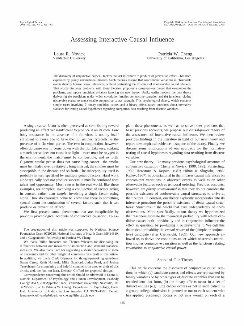
Figure 1. An illustration of the independent influences of two generativecauses on an effect occurring in entities that are presumed to recovercompletely from the influence of one cause before being exposed to asecond one. This illustration adopts the perspective of an omniscient beingto whom causal relations are visible. Letters r, s, . . ., z label individualentities.

456 NOVICK AND CHENG

situations: There are two causes of effect e that do not interact witheach other, nor with other causes of e. These figures depictidealized situations in which the relative frequencies of events(e.g., “e is not produced by any cause”) accurately reflect theprobabilities of those events, and the entities (represented bycircles) are assumed to recover completely from the influence ofthe first cause, i, before being exposed to the second cause, j.1

Figure 1 illustrates independent causal influence for the situationin which i and j each produce e (with some probability), seen fromthe perspective of an omniscient being to whom causal relationsare visible (visibility is represented in the figure by marking causesof the effect in an entity). Figure 2 illustrates the situation in whichthese causes each prevent e (with some probability), seen from theperspective of a mere mortal who must infer causal relations fromobservations. The independent influence of i and j on e illustratedin these figures should be compellingly intuitive; yet, no previ-ously proposed account of conjunctive causation, psychological ornormative, concurs with these intuitions.

Let us examine Figure 1 more closely. For simplicity, assumethat all candidate causes alternative to i, j, and their potential

interaction have no power to influence e. The outcome for a set ofentities that is consistent with this assumption is shown in the firstpanel: When the entities were exposed to neither i nor j, none ofthem showed e. Here and elsewhere, a light gray ring indicates theabsence of e in an entity. The second panel shows that i producese in two thirds of the entities. Analogously, the third panel showsthat j produces e in one third of the entities. As the figure shows,this one-third probability (of having black rings in the third panel)applies both to the entities that did not show e when i was present(the light gray rings in the second panel) and to those that did (thedark gray filled circles in the same panel), which is consistent withthe notion of the independent causal influences of i and j on e.2

Now, if i and j indeed independently produce e, then if they hadbeen both present, their individual influences would have simplysuperimposed on each other, as shown by the superimposition ofthe second and third panels in the bottom panel. In accord withintuition, for e to fail to occur in an entity in this case, e must failto be produced by i and fail to be produced by j. In this figure,not-e is the observable outcome that, in the bottom panel, exhibitsa conjunction of events from the earlier panels. Thus, applyingprobability theory to the situation depicted, the probability of e notbeing produced in the bottom panel of Figure 1 (two ninths, asshown) is the product of the probability that e is not produced byi when i is present (one third, as shown in the second panel) andthe probability that e is not produced by j when j is present (twothirds, as shown in the third panel). Note that this product defini-tion of independence does not, and intuitively should not, apply tothe event that e occurs in the presence of i and j, because e occurswhen it is produced by i, j, or both. Rather, it applies to the“nonevents,” the entities that are untouched by the causal pro-cesses in question. In this situation, the nonevent is the nonoccur-rence of e. (The product definition also applies to the conjunctionof “e produced by i” and “e produced by j” in Figure 1, indicatedby the black rings superimposed on the dark gray circles in thebottom panel. But, this conjunction is observable to an omniscientbeing only, as assumed in the figure.)

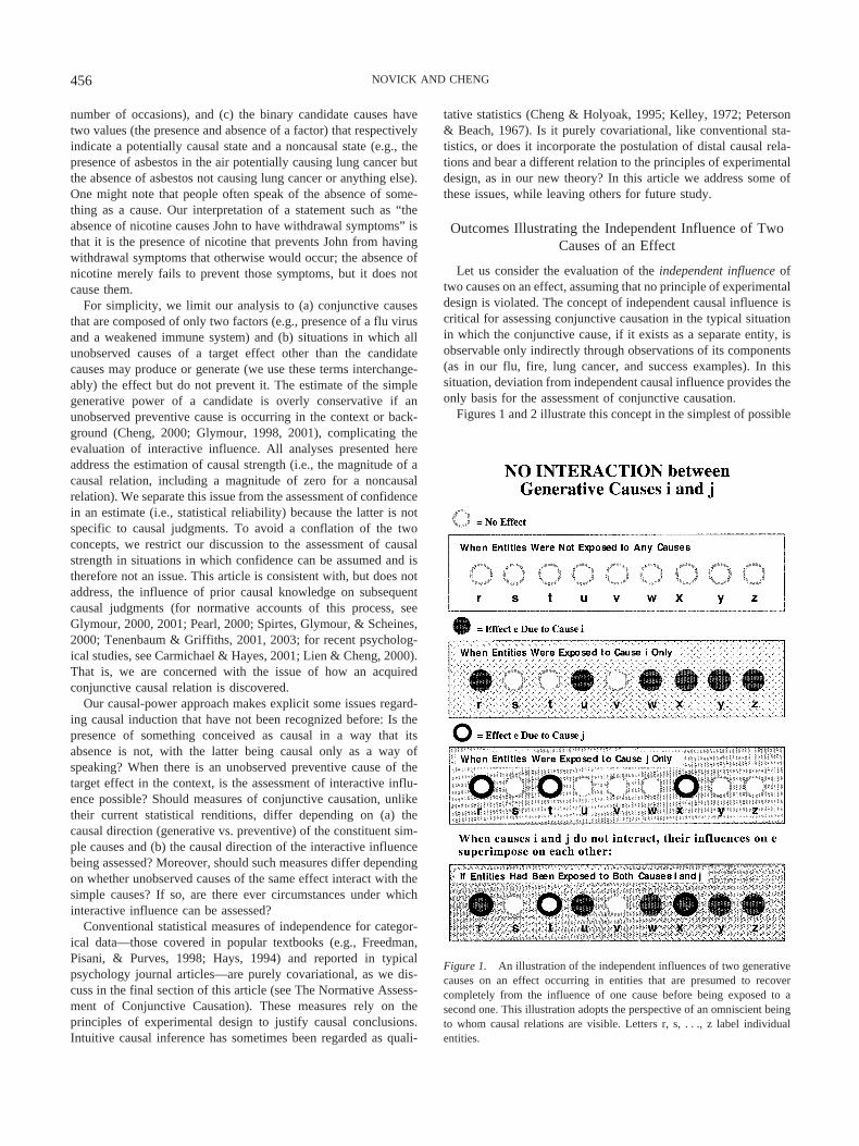
Let us now turn to Figure 2, which illustrates the independentinfluence of two preventive causes on e. For simplicity in this case,assume that candidate causes alternative to i, j, and their potentialinteraction always produce e. Thus, e occurred in every entity thatwas exposed to these alternative causes, as shown by the dark grayfilled circles in the first panel. As should be clear, the preventivesituation in this figure is a direct analogue of the generative one inFigure 1. Instead of i producing e in two thirds of the entities, inow prevents e in two thirds of the entities. Instead of j producinge in one third of the entities, j now prevents e in one third of theentities. And, as before, if i and j indeed independently prevent e,then if they had been both present, their individual preventiveinfluences would have superimposed on each other, as shown inthe bottom panel.

1 We thank Terry Au for inspiring the counterfactual wording in thesefigures.

2 In probability theory, if two events are independent, the probability oftheir conjunction is the product of the probabilities of the constituent events(Feller, 1957). This product definition implies that the probability of oneevent remains constant regardless of whether the other event occurs. Weapply this definition to causal events here.

Figure 2. An illustration of the independent influences of two preventivecauses on an effect occurring in entities that are presumed to recovercompletely from the influence of one cause before being exposed to asecond one. This illustration adopts the perspective of a mere mortal whomust infer causal relations from observations. Letters r, s, . . ., z labelindividual entities.

457INTERACTIVE CAUSAL INFLUENCE

In this case, however, for e to occur, it must not be prevented byi and not be prevented by j. Thus, the probability of e in the bottompanel of Figure 2 (two ninths, as shown) is the product of theprobability that e is not prevented by i when i is present (one third,as inferred from the first two panels) and the probability that e isnot prevented by j when j is present (two thirds, as inferred fromthe first and third panels). Notice that the product definition ofindependence now applies to the occurrence of e, which is thenonevent in this preventive situation.

How would a formal account of conjunctive causation explainand predict the compelling intuitions of independent causal influ-ence illustrated in these figures? We first review the predictions ofprevious psychological models of this process. Near the end of thearticle (see The Normative Assessment of Conjunctive Causation),we review what is predicted by the cross-product ratio (see Equa-tion 26 for its definition), the criterion of independence underlyingall conventional statistical measures for categorical data that wouldbe applicable to the causal hypotheses in question.

Purely Covariational Models Fail: The Case of theProbabilistic Contrast Model

Cheng and Novick’s (1990, 1992) probabilistic contrast model,which explains conjunctive causal attributions better than anyalternative explicit psychological model of conjunctive causes(e.g., Forsterling, 1989; Hewstone & Jaspars, 1987; Hilton &Slugoski, 1986; Kelley, 1967), nonetheless fails to account for thecompelling intuitions of independent influence in Figures 1 and 2,as we show in the following paragraphs. The other models, be-cause they do not accept quantitative input, are not applicable tothese figures.

The probabilistic contrast model attempts to explain how peopleinduce both simple and conjunctive causes. According to thismodel, reasoners evaluate whether a single causal factor, which isperceived to occur before an effect, is a simple cause of that effectby using a main-effect contrast within a focal set. The focal set isa set of events that the reasoner uses as input to the causaldiscovery process. Experimental evidence independent of subjects’causal inferences shows that their focal sets may be either larger orsmaller than the set of events specified by an experimenter (Cheng& Novick, 1990; Novick, Fratianne, & Cheng, 1992). The main-effect, or simple, contrast for candidate cause i with respect toeffect e is defined as

�Pi � P�e�i� � P�e��i �, (1)

where P(e|i) and P(e|�i ) are, respectively, the probability of e giventhe presence of i and that probability given the absence of i. Bothconditional probabilities are directly estimable by observable fre-quencies, and �Pi is a measure of covariation between i and e.Cheng and Holyoak (1995) and Melz, Cheng, Holyoak, and Wald-mann (1993) modified the model by specifying that the focal setsreasoners prefer for computing simple contrasts are those in whichevery plausible alternative cause remains constant.

When applied to the focal set consisting of the first two panelsof Figure 1, Equation 1 predicts that i causes e. Likewise, thisequation predicts that j causes e in the same figure and that i andj each prevents e in Figure 2. So far, the figures are not problematicfor the model.

Continuing with the description of the model, a two-way inter-action contrast evaluates a pair of candidate causes, which areperceived to occur before e, as a conjunctive cause of e within afocal set. This contrast for candidate causes i and j with respect toe is defined as

�Pij � �P�e�ij� � P�e��ij�� P�e�i�j� � P�e��i�j��. (2)

This contrast is thus a difference between differences—the simplecontrast for i when j is present minus the simple contrast for i whenj is absent. If �Pij is noticeably greater than zero, then i and jinteract to produce e; if it is noticeably less than zero, the twocandidates interact to prevent e. Otherwise, the influences of thetwo candidates on e are independent. Equation 2 coincides exactlywith a primary measure of interactive influence in epidemiologydiscussed in a well-regarded textbook (Rothman & Greenland,1998).

When applied to the four panels in each figure, Equation 2yields an interaction contrast value of –2/9 for Figure 1 (implyingthat i and j interact to prevent e) and 2/9 for Figure 2 (implying thati and j interact to produce e). This equation therefore fails toexplain the intuition that the figures depict independent causalinfluence.3

As we hope to show in this article, this failure stems from thelack of explicit representation of distal causal relations in purelycovariational models of (simple and conjunctive) causation. An-other shortcoming of such models traceable to the same source isthe failure to distinguish between covariation and causation. Con-sider an example in which the covariation between the conjunctionof two events and an effect in question does not indicate causation:Daffodils blooming and morning school bells ringing, in combi-nation, covary with flattened snakes on the road (the effect inquestion), even though each event individually is only very weaklyassociated (if at all) with flattened snakes. From the covariationbetween that combination of events and flattened snakes, would areasoner conclude that the conjunction of blooming daffodils andmorning school bells causes dead snakes on roads? We think not.(The pattern is due to snakes being especially likely to sun them-selves on the warm asphalt on spring mornings.)

In our view, the remedy for both shortcomings of purely co-variational models is to treat observable frequencies as manifes-tations of an underlying causal process, as in our theory of con-junctive causal power. Our theory is an extension of Cheng’s(1997) theory of simple causal power, reviewed in the next section.

A Causal-Power Theory of Covariation for Simple Causes

Cheng (1997) proposed a theory of causal discovery with re-spect to simple causes involving a single factor. According to hertheory, reasoners interpret their observations of covariation be-tween two variables, a candidate cause and an effect, in which thecandidate cause is perceived to occur before the effect, in terms of

3 Cheng and Holyoak’s (1995) modification for simple causes does nothelp here, as it is not obvious how the modification could apply. Withrespect to the conjunctive candidate, the two constituent simple causes arealternative causes; a moment’s reflection will reveal that it is impossible tohold both of these alternative causes constant while varying the presenceversus absence of the conjunctive cause.


a (probably innate) a priori framework that postulates the possibleexistence of cause-and-effect relations (cf. Kant, 1781/1965). Thisframework specifies that causes influence the occurrence of aneffect, either producing or preventing it, with certain theoreticalprobabilities, termed causal powers (Cartwright, 1989). These aredistal properties of causal relations that give rise to one’s obser-vations but exist independently of them. The generative power ofcandidate cause x with respect to effect e, denoted by qx, is theprobability with which x produces e when x occurs; the preventivepower of x with respect to e, denoted by px, is the probability withwhich x prevents (an otherwise occurring) e when x occurs. Thereasoner has a tacit goal of estimating the magnitude of thesepowers.

Motivation

Cheng’s (1997) theory specifies, under a set of assumptions,how a reasoner can discover a causal relation, rather than merelya covariational relation, from observations in the input. Of the twoprevious approaches to causal induction, the covariation approach(e.g., Cheng & Novick, 1990, 1992; Rescorla & Wagner, 1972)has been unable to either specify or justify the conditions underwhich covariation reveals causation, and the power or mechanismapproach (e.g., Ahn, Kalish, Medin, & Gelman, 1995; Shultz,1982) has been unable to specify the process that transformsinformation from the available noncausal input to a causal judg-ment (for discussions, see Cheng, 1993; Glymour & Cheng, 1998).

To understand these problems with the two previous ap-proaches, one should note that causal relations (unless innatelyknown) must be discovered on the basis of (perceptually or intro-spectively) observable events—the ultimate source of informationabout the world (Hume, 1739/1987). This constraint poses a prob-lem for all accounts of causal discovery: Observable characteris-tics typical of causation do not always imply causation. As wedemonstrated in our snake example, covariation need not implycausation. Nor does the absence of covariation between a candi-date cause and an effect imply the lack of a causal relation betweenthem, even when alternative causes are controlled. Consider anexperiment testing whether a candidate cause i prevents an effecte. Suppose alternative causes of e are controlled, and e occursneither in the presence of i nor in its absence, so that there is nocovariation between i and e. For example, suppose headaches (theeffect) never occur in patients who are given a potential drug forrelieving headaches (the candidate) or in patients who are given aplacebo. The reasoner would not be able to conclude from thisabsence of covariation that the drug does not relieve headaches—there is no room for the drug to reveal its preventive power.

A Synopsis

According to Cheng’s (1997) power PC theory (short for“causal-power theory of the probabilistic contrast model”), toevaluate the power of a candidate cause i to influence effect e,reasoners partition all causes of e into i and the composite of(known and unknown) causes of e alternative to i, labeled a, andthey explain covariation defined in terms of observable frequen-cies by the hypothetical unobservable powers of i and a. Thepartitioning of all causes of e into i and a is the simplest possible

conception of the causes of e that would still explain covariationbetween i and e.

The assumptions underlying the derivation of simple causalpower are as follows:

1. i and a influence e independently,

2. causes in a could produce e but not prevent it,4

3. the causal powers of i and a are independent of theiroccurrences (e.g., the probability of a both occurring andproducing e is the product of the probability of a occur-ring and the power of a), and

4. e does not occur unless it is caused.

As we show in the following paragraphs, from these four as-sumptions one can derive a necessary condition for inferring thecausal power of i. This condition, which we call the no-confounding condition, concerns the independent occurrence of iand a.5 Assumptions 1 and 2, like the no-confounding condition,are merely working hypotheses, and each is adopted or not de-pending on perceived evidence for or against it.

When e occurs at least as often after i occurs as when i does notoccur (a condition that can be determined by observation alone), sothat �Pi � 0, reasoners evaluate the hypothesis that i produces e,and they estimate the generative causal power of i. To do so, theyallow the possibility that i produces e and explain P(e|i) by theprobability of the union of two events: (a) e produced by i and (b)e produced by a if a occurs in the presence of i. That is, they reasonthat when i is present, e can be produced by i or by a if a occursin the presence of i. Likewise, they explain P(e|�i ) by how often eis produced by a alone when a occurs in the absence of i.

Figure 3 illustrates these explanations of the two conditionalprobabilities by Euler circles. The dashed and undashed circles inthe figure, respectively representing e produced by i and e pro-duced by a, are both unobservable; they are theoretical constructs.Only the white and shaded areas—respectively representing eoccurring and e not occurring—and in which of the two boxesthese events occur—the two boxes respectively representing ex-posure to i and no exposure to i—can be observed. Now, eoccurring in the presence of i—the white area in the left boxrepresenting the union of the dashed and undashed circles—can bedecomposed theoretically into the sum of the area of the dashedcircle and that of the undashed circle, minus their overlap. Thedashed circle in this box (i.e., how often e is produced by i wheni is present) depends on how often i occurs (always in this situa-tion) and its causal power, qi (i.e., how often i produces e), atheoretical unknown. The undashed circle can be similarly ex-

4 Glymour (1998, 2000) notes that a weaker assumption—that no unob-served causes in the composite a prevent e—would suffice for inferring thepower of i. On this assumption, if the reasoner conditionalizes on theabsence of any observed preventive causes of e (i.e., restricts the focal setto events in which observed preventive causes of e are absent), then the“explanations” of P(e|i) and P(e|�i ) in Cheng’s (1997) theory (sketched inthe paragraphs that follow these assumptions ) would apply.

5 We thank Clark Glymour and Patricia Kitcher for suggesting theterminology that we adopt here for some of Cheng’s (1997) assumptions.


plained. Likewise, the white area in the right box can be analo-gously explained, in this case by how often e is produced by a inthe absence of i (see the equations in Figure 3). These explanationsof e set up equations relating the observable quantities to thevarious theoretical variables.

For situations in which �Pi � 0 (e occurs at most as often afteri occurs as when i does not occur, as can be determined byobservation alone), there are analogous explanations for evaluatingpreventive causal power. The only difference in the preventivecase is that reasoners evaluate the hypothesis that i prevents erather than i produces e. This difference implies that when reason-ers evaluate whether i prevents e, they explain P(e|i) by theprobability of the intersection of two events: (a) e produced by aif a occurs in the presence of i and (b) e not stopped by i. That is,they reason that when i is present, e occurs only if it is bothproduced by a and not prevented by i. The explanation of P(e|�i )remains as before.

The goal of these explanations of P(e|i) and P(e|�i ) is to yield anestimate of the (generative or preventive) power of i from observ-able frequencies alone, even though it may never be possible toobserve the influence of i in isolation. (For Figure 3, this goalwould correspond to estimating the whole of the dashed circlewhen i is present, even though there may never be a diagramshowing that circle by itself.) These explanations show that, undersome conditions but not others, covariation implies causation. Inparticular, when a and i do not occur independently—that is, whenthere is confounding (e.g., between a rooster’s crowing and thetrue cause of sunrise)—one equation in four unknowns results. Inthis case, therefore, there is no unique solution for the desiredunknown. That is, the observed value of �Pi does not allow anyinference about the causal efficacy of i: �Pi may be greater or lessthan the causal power of i (Cheng, 2000).6

But, consider the special case in which a occurs independentlyof i (i.e., when there is no confounding). Under this condition,these explanations yield equations with only one unknown, thecausal power of the candidate.7 Equation 3 gives an estimate of qi,the generative simple power of i, when �Pi � 0:

qi ��Pi

1 � P�e��i� ;8 (3)

and, Equation 4 gives an estimate of pi, the preventive simplepower of i, when �Pi � 0:

pi ��Pi

P�e��i� . (4)

Note that the righthand sides (RHSs) of Equations 3 and 4 requireobservations regarding i and e only, implying that qi and pi can beestimated without observing a.

Intuitively, Equations 3 and 4 make sense as respective esti-mates for simple generative and preventive power. Recall that qi isthe distal probability with which i produces e. In Equation 3, thisprobability is estimated by how often e occurs in the presence ofi among entities in which e is not already produced by alternativecauses. To see this interpretation, note that when a occurs inde-pendently of i, e is produced by a just as often whether or not i ispresent. Therefore, P(e|�i) estimates how often e is produced by awhen i is present (as well as when i is absent). Accordingly, 1 �P(e|�i ), the denominator on the RHS of Equation 3, provides anestimate of how often e is not already produced by a when i ispresent.

As should be clear, at one extreme, qi 1 means that i isestimated to produce e in every entity. At the other extreme, qi

6 Generalizations of Cheng’s (1997) theory have been shown to allowgenerative causal power to be estimated normatively in certain cases evenwhen there is confounding (Glymour, 2001). For the rooster example,although no inference results from applying a causal-power analysis to“crowing” with respect to “sunrise,” a typical reasoner would judge thatcrowing does not cause sunrise. Cheng gave an explanation of how thisdefinite answer might be due to previously inferred causal knowledge (seealso Lien & Cheng, 2000).

7 A nice property of causal powers is that the solutions are independentof the particular covariation measure “explained” by such powers when-ever there is a solution according to the explanations. For example, ex-plaining the ratio of P(e|i) to P(e|�i ) instead of the difference between theseconditional probabilities yields identical values for the candidate causalpower except for cases in which the ratio explanation gives an undefinedvalue.

8 Equations 3 and 4 appear in Sheps’s (1958) article, in which Shepsrefers to them as estimates of harmful effects and beneficial effects,respectively. Equation 3 was subsequently derived from assumptions sim-ilar to those in Cheng (1997) and proposed as a measure of susceptibilityby Khoury, Flanders, Greenland, and Adams (1989). It was also derived byPearl (2000) under a weaker set of assumptions, with a differentinterpretation.

Figure 3. Euler diagrams illustrating the explanation of covariation in Cheng’s (1997) theory of simple causalpower.


0 means that i is estimated to never produce e in any entity (i.e., tobe noncausal). Of course, if e occurs all the time due to a (i.e.,P(e|�i ) 1), qi cannot be assessed (i.e., it has the undefined valueof 0/0), as there are no remaining entities in which i can possiblymanifest its generative power.9 Equation 3 therefore explains thisintuition and its analogue in experimental design—the principle ofavoiding a ceiling effect. Despite the observation that �Pi 0 inthis case, on the basis of this pattern of observations one would notmake any judgments about the causal relation in the world betweeni and e, which is assumed to exist regardless of a reasoner’sobservations; in particular, one would not infer that i does notcause e. In contrast, if e never occurs due to a (i.e., nothing otherthan i produces e, so that P(e|�i ) 0), then P(e|i), which in this caseequals the simple contrast (�Pi), provides a good estimate of qi: Inthis context, whenever e occurs in the presence of i, it is producedby i. Note that, unlike purely covariational measures (e.g., �Pi),whenever qi has a defined value, that value is a property of thecausal relation between i and e and is independent of how oftenalternative causes in the context produce e (for an illustration ofthis feature of simple power, see Glymour & Cheng, 1998).

Analogously for Equation 4, the simple preventive power of i isestimated by how often e does not occur in the presence of i amongentities in which e is produced by a. As before, P(e|�i ) is anestimate of how often e is produced by a. Thus, pi 0 means thati is estimated to never prevent e in any entity, and pi 1 meansthat i is estimated to prevent e in every entity. Of course, if e neveroccurs due to a (i.e., P(e|�i ) 0), pi cannot be assessed (i.e., it hasthe undefined value of 0/0), as there are no entities in which i canpossibly manifest its preventive power. Equation 4 therefore ex-plains this intuition and the tacit preventive analogue of the ceilingeffect, as illustrated in our headache-relieving-drug example.10

This unspoken principle of avoiding situations in which e neveroccurs in the absence of a candidate in tests of its preventive poweris uniformly obeyed in experimental design (for the use of the lasttwo principles by untutored reasoners, see Wu & Cheng, 1999). Incontrast, if e occurs all the time due to a (i.e., P(e|�i ) 1), then��Pi, which now equals 1 � P(e|i), provides a good estimate ofpi: In this context, whenever e does not occur in the presence of i,it is prevented by i.

Some Implications

The power PC theory provides a qualitative description ofuntutored human causal discovery involving direct simple causes.As described in Cheng (1997), it accounts for a diverse range ofpsychological experimental findings and intuitions that are inex-plicable by previous accounts of causal inference.

A critical aspect of the power PC theory is that it “deduces”when to induce. One consequence of this is that the theory pro-vides a normative justification for when and why covariationimplies causation. In particular, it explains some principles ofexperimental design. As we just noted, it explains the ceiling effectand its preventive analogue. In addition, it explains the principle ofcontrol. To enable causal inference, scientists use methods such asrandomly assigning subjects to conditions in a study and holdingalternative causes at a constant value across conditions. The prin-ciple of controlling for alternative causes is also used in observa-tional studies, for example, by matching as much as possible therelevant properties of subjects in every pair (e.g., identical twins

raised in the same family) except for a candidate feature (e.g.,oxygen deprivation during delivery from mother) to study itsinfluence on some outcome (e.g., schizophrenia). Because thederivations of Equations 3 and 4 show that those equations resultif and only if there is no confounding (Cheng, 1997, 2000), theyexplain why no confounding is a boundary condition for causalinference according to experimental design. Thus, whereas thesebasic principles of design are extrinsic to purely covariationalmeasures, and either augment or overrule their interpretation, theyarise from the same assumptions as do the measures under ourcausal-power approach and are intrinsically incorporated into thesemeasures.

Cheng’s (1997) theory can be regarded as a particular parame-terization of directed graphical models, sometimes called Bayesiannetworks (Glymour, 1998, 2000, 2001; Pearl, 2000; Spirtes et al.,2000; Tenenbaum & Griffiths, 2001; see Gopnik et al., 2004, fora general proposal of such networks as a psychological model). Inthis parameterization, each causal-power variable is a parameterassociated with an arrow in the acyclic graph representing theassumptions underlying the theory, a parameter that represents theinfluence of (a) an intervention on the node at the tail of an arrowon (b) the node at the head of the arrow.

A Causal-Power Analysis of Two-Way Interactions

Overview and Assumptions

In this section, we extend Cheng’s (1997) power PC theory ofsimple causation to address the assessment of conjunctive causa-tion. We call our new theory the conjunctive power PC theory.11

Both of these theories propose that reasoners implicitly follow aqualitative version of the mathematical analyses. Our predictionsconcerning their judgments about causal power are thereforeordinal.

We present an analysis of how a reasoner might evaluatewhether two candidate causes, i and j, interact to influence aneffect e (i.e., whether they do not influence e independently). Justas in the case of simple causes, the reasoner explains observablecovariation by the possible causal powers. Whereas Cheng (1997)explained the occurrence of e in the presence of a single causalcandidate, i, by considering the possible existence of two causes ofe, namely, i and a (the composite of causes other than i), we mustconsider the possible existence of four causes to explain theoccurrence of e in the presence of two causal candidates, i and j:i, j, the combination of i and j as a conjunctive cause, and a (here,a is the composite of all causes other than the candidate causes i,j, and their conjunction). We refer to the power of the combinationof i and j as their conjunctive power. Table 1 enumerates which ofthese four candidate causes can exert their influence in the variouspossible situations formed by varying the presence versus absence

9 Because �Pi is nonnegative for qi, P(e|�i ) being 1 implies that �Pi 0;thus, qi 0/0.

10 It is not the typical floor effect, which concerns situations in whichsome enabling conditions of a candidate for generative—rather than pre-ventive—power are missing so that i does not increase the frequency of e.

11 PC again stands for probabilistic contrast, but in this case the contrastis the conjunctive contrast specified by our new theory (Equation 5) ratherthan the one specified by our old probabilistic contrast model (Equation 2).


of i and j. The partitioning of all causes of e into these four yieldsthe simplest possible conception of the causes of e that wouldexplain any covariation between e and the candidate causes i, j,and their conjunction.

Estimating the simple and conjunctive powers of i and j requiresthat i, j, and e be observable. Our analyses concern the typicalsituation in which the conjunctive cause is observable only indi-rectly through observations of i and j (as in all of our examples ofconjunctive causation so far). If the conjunctive cause is a newentity that is directly observable (e.g., a new chemical compoundthat is produced as the result of mixing two drugs), it can poten-tially be evaluated as a simple cause on its own, rendering thepresent analyses unnecessary. In contrast, in the situation underinvestigation here, whether i and j interact to influence e, as wenoted earlier, can only be inferred from the deviation of theobserved probability of e from that expected if i and j, possiblycounterfactually, exerted only their simple powers on e. The esti-mation of this expected probability is therefore a critical step in ouranalyses.

The role of this expected probability in the estimation of con-junctive power has a direct analogue in the estimation of simplepower. Recall that, with respect to simple powers, P(e|�i ) estimateshow often e is produced by alternative causes. In other words,P(e|�i ) estimates the expected probability of e in the presence of i,assuming that only causes other than i exerted an influence on e.A deviation from this counterfactual probability indicates that i isa simple cause of e. Likewise, we assume that to evaluate theconjunctive power of two candidate causes i and j, the reasonerestimates the expected probability of e in the presence of i and j,assuming that only causes other than the conjunction of i and jexerted an influence on e.

Thus, analogous to the simple contrast in Equation 1, a con-junctive contrast has the following general form:

�Pij � P�e�ij� � P̃�e�ij�, (5)

where P(e|ij) is the actual (i.e., observed) probability of e in thepresence of i and j, and P̃(e|ij) is the expected probability if i andj exerted only their simple powers on e. Just as reasoners explainthe two conditional probabilities in a simple contrast to “deduce”simple causal power in Cheng’s (1997) theory, they explain theanalogous conditional probabilities in Equation 5 to “deduce”conjunctive power in our extension of that theory (see Figure 4).Now, instead of partitioning the causes of e into the candidatesimple cause and everything else, reasoners partition them into thecandidate conjunctive cause corresponding to the combination of iand j (the dashed circle in Figure 4) and everything else (the simplecauses i and j, represented by two lighter undashed circles in thefigure, and a composite of all other causes of e, represented by adarker undashed circle). Reasoners explain P(e|ij) by the potentialcausal powers of i, j, their conjunction, and a; they explain P̃(e|ij)by the same set of potential causal powers without the conjunctivepower of i and j. Thus, as for simple causes, everything other thanthe candidate is common across the two conditional probabilities.Analogous to Figure 3, the goal here is to estimate the relative areaof the whole dashed circle even though it may never appear on itsown.

Recall that in Cheng’s (1997) theory, depending on the sign of�Pi, reasoners evaluate i as either a generative or preventive cause,situations that call for different measures of simple causal power.The measures of conjunctive power similarly differ depending onthe sign of �Pij, as well as of �Pi and �Pj. Allowing i and j to beeither generative or preventive causes of e, and treating i and j asinterchangeable (so that i being generative and j being preventiveis equivalent to i being preventive and j being generative), there arethree possible combinations of simple candidate cause types: Bothsimple candidate causes may be potentially generative, both maybe potentially preventive, and one may be of each type. For eachof these three combinations of simple cause types, the conjunctionof i and j may either generate e or prevent it. There are, therefore,six possible combinations of two simple powers and their conjunc-tive power.

For a concrete illustration, consider an example of the lastcombination of candidate cause types. The effect of interest (e) isattending (as opposed to not attending) a high school basketballgame in a Midwestern state. Snow-covered roads (i) reduce atten-dance (i.e., have a preventive influence), whereas a strong winningrecord for the home team (j) increases attendance (i.e., has a

Table 1Possible Causes of an Effect, e, in the Various PossibleSituations Involving Observable Candidate Causes i and j WhenAll Alternative Candidate Causes (Known and Unknown),Denoted by the Composite a, Influence e Independently ofi and j

i

j

Occurs Does not occur

Occurs i ∧ j, i, j, a i, aDoes not occur j, a a

Note. i ∧ j denotes the conjunctive cause composed of both i and j.

Figure 4. Euler diagrams illustrating the explanation of covariation in our theory of conjunctive causal power.


generative influence). The identification of these simple causesmay not provide a sufficient explanation, however, because snowyroads and a strong winning record may interact to influenceattendance, such that the combination, for example, increases theprobability of attending compared with what would be expected ifthe candidates exerted only their simple powers.

For each of the three combinations of the types of simple powersof i and j, we present an explanation of P̃(e|ij) based on the sameassumptions listed earlier for the derivation of simple power,applying them to simple causes only, including the two candidatesimple causes, i and j. The results concerning P̃(e|ij) thereforefollow directly from Cheng’s (1997) theory of simple power.

Then, for each of the three combinations of simple powers, wederive equations for qij and pij, respectively the generative andpreventive powers of the conjunction of i and j. We do so byintroducing explanations of the observed P(e|ij), completing theexplanation of the conjunctive contrast (Equation 5). Our deriva-tions make use of Assumption 1 below, which concerns conjunc-tive causal power, together with the simple-power assumptions,which are generalized when relevant to apply not just to i but alsoto the other two candidate causes, j and the conjunction of i and j.We list all five relevant assumptions below, with the last fourmapping, respectively, onto the four simple power assumptions:

1. The influence of the interaction between i and j can berepresented by a separate conjunctive power, qij or pij;this conjunctive cause can operate only when i and j bothoccur (analogously as for simple causes).

2. All causes, simple and conjunctive, influence eindependently.

3. Unobserved causes in a could produce e, but not preventit.

4. All causes influence the occurrence of e with causalpowers that are independent of how often the causesoccur.

5. e does not occur unless it is caused.

The results of our mathematical derivations, detailed in theremainder of this section, are summarized in Figures 5 and 6, forthe special case in which a occurs independently of i, j, and theirconjunction (i.e., when there is no confounding). Because theexplanation of P̃(e|ij) involves only a subset of the assumptionsjust listed for conjunctive power, our accounts of P̃(e|ij) and ofconjunctive power should be evaluated separately; our account ofconjunctive power could fail to hold even when our account ofP̃(e|ij) is supported. We propose, however, that each of these partsof our theory is both descriptive and normative.12

Both Candidate Causes Are Generative

First, we consider situations in which candidate causes i and jeach (potentially) produces e (e.g., see Figure 1). That is, these aresituations in which �Pi � 0 and �Pj � 0. In these situations, wedenote the expected probability of e when both i and j are presentbut exerted only their simple powers on e by P̃(e|ij), with the

subscript indicating that the simple candidate causes are bothpotentially generative.

Estimating P̃(e|ij)

If i and j exerted only their simple powers on e, then when i andj are jointly present, e occurs if i causes e, j causes e, or a is presentand causes e. Accordingly, the expected probability of e in thepresence of i and j can be estimated by the union of these threeevents. A simple way to calculate this probability makes use of therelevant De Morgan’s Law.13 Specifically, negating both sides ofthe law that states that the complement of a union is the intersec-tion of the complements of the constituents of the union, we findthat P̃(e|ij) is the complement of the probability of the inter-section of three events in the presence of i and j: e is not producedby i, e is not produced by j, and e is not produced by a when a ispresent. In other words, when i and j are both present but theyexerted only their simple influences, the expected probability of eis the complement of the probability that e is not produced by anyof the simple candidate causes. Therefore,

P̃�e�ij� � 1 � �1 � qi� � �1 � qj� � �1 � P�a�ij� � qa�. (6)

Equation 6 contains unobservable causal-power variables andthe probability P(a|ij), which is typically unobservable because a isnot knowable. To demonstrate that the equation is solvable throughobservations alone, and hence there is no circularity in our argu-ment, we replace the unobservable terms with “observable” prob-abilities, that is, with probabilities that are directly estimable byobservable frequencies.

To do so, we first estimate the simple powers, qi and qj,according to Cheng’s (1997) theory. Recall that the power of asimple candidate cause can be estimated from observable proba-bilities using Equations 3 or 4 only under the no-confoundingcondition, namely that all causes alternative to the candidate causeoccur independently of it. In the situation of interest here, satisfy-ing this condition would mean that, for example, when i is thecandidate cause, j, a, and the conjunctive cause must all occurindependently of it. This implies that even for the special case inwhich a occurs independently of i, j, and their conjunction, toestimate the simple power of i or j, conditionalizing on the absenceof the other simple candidate is the only way one can be sure thatthe no-confounding prerequisite is satisfied (see Table 1). Withoutthis conditionalization, confounding may occur: For example, with

12 The independent influence assumption can be met in two ways. Onepossibility is that the simple causes and the conjunctive cause operatesequentially, with the conjunctive cause exerting its influence, if any, onthe outcome produced by the simple causes. The other possibility is that thesimple and conjunctive causes operate in parallel. We discuss this distinc-tion more fully later (see The Assumption That the Conjunctive CauseOperates on the Static Outcome of the Simple Causes), as it is relevant foronly two of the six possible cases of conjunctive causation. We take thesequential version of Assumption 1 to be the default.

13 De Morgan’s Laws state that the complement of a union is theintersection of the complements of the constituents of the union (e.g.,not-a-or-b � not-a and not-b) and that the complement of an intersectionis the union of the complements of the constituents of the intersection (e.g.,not-a-and-b � not-a or not-b).


respect to candidate i, the conjunctive cause, if it exists, wouldcovary with i, occurring in its presence but not in its absence.

Accordingly, for qi, we instantiate Equation 3 conditional on jbeing absent, yielding

qi �P�e�i�j � � P�e��i�j �

1 � P�e��i�j� . (7)

Likewise,

qj �P�e��ij� � P�e��i�j �

1 � P�e��i�j� . (8)

Because qi and qj have undefined values when P(e��i�j) 1, analo-gously as we showed earlier regarding the ceiling effect for simplecauses, P(e��i�j) � 1 is a condition for estimating these simple powers.

The last unobservable term in the expression for the expectedprobability (see Equation 6) is the product P(a�ij) � qa. When aoccurs independently of the conjunction of i and j (i.e., when the

no-confounding condition holds), P(a|ij) P(a��i�j ). Thus, anal-ogous to the explanation of P(e��i ) by P(a) � qa in Cheng(1997), we obtain

P�a�ij� � qa � P�a��i�j � � qa � P�e��i�j�. (9)

Expanding the expression for the expected probability (seeEquation 6) using Equations 7–9 and simplifying, we obtain Equa-tion 10, which does not contain any unobservable variables. Toshow more clearly the analogous forms among the equations weobtain, we express the RHS of this equation in terms of theprobability of not-e rather than of e:

P̃�e�ij� � 1 �P�e��i�j � � P�e��ij�

P�e��i�j � . (10)

Note that without the no-confounding condition—that a occursindependently of i, j, and their conjunction—Equations 7–9 would

Figure 5. Theoretical equations for assessing interactive causal influence for the special case in whichalternative causes occur independently of the candidate causes.


not obtain, leaving P̃(e|ij) in Equation 6 unsolved.14 Anticipatingour subsequent derivations, without a solution for P̃(e|ij), therewould be no solution for conjunctive causal power. In other words,when there is confounding of the causes in question by alternativecauses of the effect, our measure indicates that there is no solutionfor conjunctive power. Thus, as for simple causal power, ourderivations explain why no confounding is a boundary conditionfor inferring conjunctive causal power.

This explanation reveals, as do analogous explanations inCheng’s (1997) theory, a new relation between the principles ofexperimental design and the mathematical measures of inference.Contrary to current scientific practice, in which the output ofstatistics is overridden when a principle of experimental design isviolated, under our approach the mathematical measure yields anoutput that corresponds to the intuitively and normatively correctinference, so that there is no such overriding: The design principlesthat concern causality become part and parcel of the mathematicalmeasures of inference.

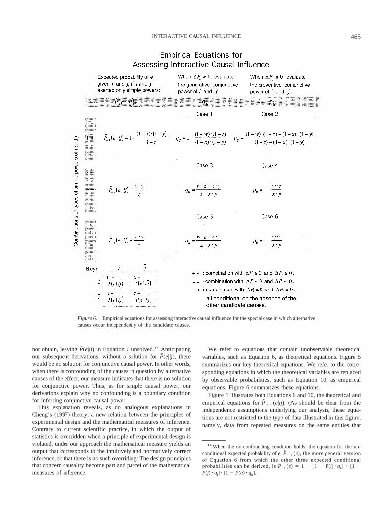
We refer to equations that contain unobservable theoreticalvariables, such as Equation 6, as theoretical equations. Figure 5summarizes our key theoretical equations. We refer to the corre-sponding equations in which the theoretical variables are replacedby observable probabilities, such as Equation 10, as empiricalequations. Figure 6 summarizes these equations.

Figure 1 illustrates both Equations 6 and 10, the theoretical andempirical equations for P̃(e|ij). (As should be clear from theindependence assumptions underlying our analysis, these equa-tions are not restricted to the type of data illustrated in this figure,namely, data from repeated measures on the same entities that

14 When the no-confounding condition holds, the equation for the un-conditional expected probability of e, P̃(e), the more general versionof Equation 6 from which the other three expected conditionalprobabilities can be derived, is P̃(e) 1 � [1 � P(i) � qi] � [1 �P(j) � qj] � [1 � P(a) � qa].

Figure 6. Empirical equations for assessing interactive causal influence for the special case in which alternativecauses occur independently of the candidate causes.


recover from the influence of each cause. They are also applicableto other types of data for which those independence assumptionshold—for example, data from exposing disjoint sets of entities tothe various combinations of candidate causes.) Substituting thecausal-power values from Figure 1 into the theoretical equationyields the value of the expected frequency shown in the bottompanel of the figure: P̃(e|ij) 1 � (1 � 2/3) � (1 � 1/3) � (1� 0) 7/9. Substituting the corresponding relative fre-quencies from the top three panels of that figure into theempirical equation yields the same value:

P̃�e�ij� � 1 �1/3 � 2/3

1 � 0� 7/9.

(The power values and observed relative frequencies happen tocorrespond in this simple figure, because i and j are the only causesof e.) As can be seen, our mathematical criterion of independentinfluence corresponds to the intuitive one illustrated in Figure 1.

As for simple causes, we assume that the direction of theconjunctive causal hypothesis to be evaluated—that the conjunc-tion produces e or that it prevents e—depends on the sign of theconjunctive contrast (Equation 5). For �Pij � 0 and �Pij � 0,respectively, the reasoner assesses generative and preventive con-junctive power. We discuss these two cases below. When �Pij 0, the reasoner may evaluate either type of conjunctive power orboth types. (Recall that the goal is to solve for the causal powers,which may be either zero or undefined when �Pij 0.)

Case 1: Evaluating the Conjunctive Power of i and j toProduce e, When i, j, and a May Each Have SimpleGenerative Power

The derivation of qij. We first consider the case in which �Pij

� 0, so that the reasoner assesses whether i and j interact toproduce e and estimates qij, the generative power of the conjunc-tion. In this case, the observed P(e|ij) would be explained by howoften e is produced in the presence of i and j by the simple causesor by the conjunction of i and j. Note that including the conjunctivepower as a possible explanation for P(e|ij) does not presupposethat the conjunction is in fact a cause, as its power may turn out tobe zero. Applying Assumptions 1–5 and the relevant De Morgan’sLaw, one can see that the probability of this union is the comple-ment of the probability of the intersection of two events in thepresence of i and j: e is not produced by the simple causes, and eis not produced by the conjunction of i and j:

P�e�ij� � 1 � �1 � P̃�e�ij�� 1 � qij�. (11)

Substituting the expression for P(e|ij) from Equation 11 into theconjunctive contrast defining �Pij (Equation 5), simplifying, andrearranging terms, we obtain an expression for generative conjunc-tive power:

qij ��P

1 � P̃�e�ij�. (12)

Expanding P̃(e|ij) in Equation 12 according to the theoreticalequation for the expected probability (Equation 6), simplifying,and making use of the no-confounding condition (independentoccurrence) to reduce P(a�ij) to P(a), we obtain

qij ��P

�1 � qi� � �1 � qj� � �1 � P�a� � qa�. (13)

These results show that qij has a defined value only undercertain (observable) conditions. As can be seen from Equation 12,qij has a defined value only if P̃(e�ij) � 1. Equation 13clarifies that this condition obtains only if neither a nor i norj produces e all the time, implying that P(e��i�j ) � 1, P(e�i�j ) � 1,and P(e��ij) � 1.

The interpretation of qij. The analogy between the equationsfor conjunctive and simple power (Equations 12 and 3, respec-tively) should be clear. Just as 1 � P(e|�i ) in Equation 3 is anestimate of how often e is not already produced by causes otherthan the one of interest, so too is 1 � P̃(e�ij) in Equation 12.Other causes consist of a only for Equation 3, but consist of thesimple causes i and j as well as a for Equation 12. Therefore, thegenerative power of a candidate cause, both simple and conjunc-tive, is estimated by how often e occurs in the presence of thecandidate among entities in which e is not already produced byalternative causes.

To visualize generative conjunctive power, one should imaginesuperimposing the influence of the conjunctive cause on the bot-tom panel of Figure 1, so that this panel depicts the observedP(e|ij) rather than the expected P̃(e|ij). Assume that some of theentities (say, a randomly selected set) have sun rays radiating fromthem, denoting the occurrence of e due to the conjunctive cause, asseen by the omniscient being. Some of the entities so marked willbe ones in which e is not already caused by the simple causes (i.e.,the light gray rings); qij would be estimated by the proportion ofshining rings among the light gray ones. As the visualizationshows, qij is a probability (on a ratio scale) that has a well-definedmeaning in terms of the relative frequency of an event in the world.As we discuss later (see On the Interpretability of the Output ofVarious Measures of Interactive Causal Influence), this is notalways true of the causal estimates generated by purely covaria-tional models.

We interpret our result regarding qij as a psychological model intwo ways. The first, indirect, interpretation is rooted in the expres-sion of conjunctive power in terms of theoretical power variables.According to this interpretation, a reasoner may estimate thenumerator on the RHS of Equation 12, �P, according to Equa-tion 5. In turn, P̃(e|ij) is estimated according to Equation 6, withqi, qj, and P(a|ij) � qa estimated according to Cheng’s (1997)theory (see Equations 7–9).

The second, more direct, interpretation makes use of anotheranalogy to Cheng’s (1997) solutions for simple power by consid-ering conjunctive power purely in terms of observable probabili-ties. To arrive at this interpretation, we expand the theoreticalequation for conjunctive power (Equation 12) according to theconjunctive contrast equation and the empirical equation for theexpected probability (Equations 5 and 10, respectively). Simplifi-cation yields an empirical equation for qij when i and j arepotentially generative:

qij � 1 �P�e��ij� � P�e��i�j �P�e��i�j � � P�e��ij�. (14)

The conditions for applicability for Equation 14 are necessarily thesame as those for Equation 13—the theoretical expression for qij in


this situation—because the two equations are algebraically equiv-alent. When i and j do not interact,

P�e��ij� � P�e��i�j �P�e��i�j � � P�e��ij� � 1,

and qij 0. We illustrate Equation 14 for this special case byreturning to Figure 1. Instantiating this equation with the condi-tional probabilities estimated from that figure yields

qij � 1 �2/9 � 9/9

3/9 � 6/9� 0.

Although the two procedures for estimating conjunctive powergive identical estimates of qij, the indirect procedure seems moreplausible to us. We do not empirically differentiate between themin this article, however, because our goal here is to study whatreasoners compute, rather than how they compute it (Marr, 1982).

Case 2: Evaluating the Conjunctive Power of i and j toPrevent e, When i, j, and a May Each Have SimpleGenerative Power

The derivation of pij. Now consider the case in which �Pij �0, so that the reasoner evaluates whether i and j interact to prevente; that is, the reasoner estimates pij, the preventive power of theconjunction. As in Case 1, i, j, and a may each individuallygenerate e; thus, P̃(e|ij) remains as given by Equation 6.

If i and j potentially interact to prevent e, then in the presence ofi and j, e would occur if it is (a) produced by the simple causes and(b) not prevented by the conjunctive cause. Thus, the observedP(e|ij) would be the probability of the intersection of these twoevents, yielding

P�e�ij� � P̃�e�ij� � �1 � pij�. (15)

Substituting the expression for P(e|ij) from Equation 15 into theconjunctive contrast (Equation 5), simplifying, and rearrangingterms, we obtain a theoretical expression for pij in this situation:

pij ��P

P̃�e�ij�. (16)

Rewriting the RHS of Equation 16 in terms of observable proba-bilities as we did for Case 1, we obtain an empirical equation forpij in this situation:

pij �P�e��ij� � P�e��i�j � � P�e��ij� � P�e��i�j �

P�e��i�j � � P�e��ij� � P�e��i�j � . (17)

When i, j, and a are all potentially generative, the conjunctivepowers ( pij and qij) are expressed most directly in terms of theconditional probabilities of not-e, the nonevent. Recall that thenonevent is the outcome showing lack of influence by the simplecauses. Figure 1 illustrates the special case for Equations 16 and 17in which the observed relative frequencies yield pij 0.

The interpretation of pij. The analogy between Equation 16 forconjunctive preventive power and Equation 4 for simple preven-tive power should be clear. Both equations estimate how often e isprevented in the presence of the candidate cause among entities inwhich e is produced by causes other than the candidate. Returningto Figure 1 for a different visualization, let us superimpose the

influence of the preventive conjunctive cause on the bottom panel,and shrink entities in which e is prevented by this cause. Then, pij

would be the proportion of small entities among the seven entitiesthat currently show e.

Discriminating the Conjunctive Power PC Theory Fromthe Probabilistic Contrast Model: A DeterministicExample

Suppose e always occurs in the presence of i or j alone, neveroccurs in the absence of both causes, and always occurs in thepresence of both causes. An intuitive causal interpretation of thispattern of probabilities is that (a) i and j each always produces e;(b) they do not interact to prevent e; and (c) they may, or may not,interact to produce e—there is no evidence either way. A reasonertherefore definitely should not conclude that i and j interact.Contradicting this intuition, the interaction contrast (Equation 2)from the probabilistic contrast model (Cheng & Novick, 1990)yields the conclusion that i and j interact to prevent e, as thatcontrast has a value of �1. Our conjunctive power equations, onthe other hand, yield conclusions that are in accord with intuition:qij has an undefined value according to Equations 12 and 14, andpij 0 according to Equations 16 and 17 (because P̃(e�ij) 1and �P 0). In the empirical section of this article (seeEmpirical Tests of the Conjunctive Power PC Theory), we discusssome existing data on reasoners’ causal attributions when pre-sented with the type of information in this example.

Both Candidate Causes Are Preventive

Next, we consider situations in which each of the candidatecauses, i and j, (potentially) prevents e (e.g., see Figure 2). In thesesituations, we denote the expected probability of e when both i andj are present but exerted only their simple powers by P̃��(e|ij),with the subscript indicating that the simple candidate causes areboth potentially preventive.

Estimating P̃��(e|ij)

If i and j exerted only their simple powers on e, then when i andj are both present, e occurs if a is present and causes it, and neitheri nor j prevents it. In this situation, the expected probability of e isas shown in Figure 5 (see the leftmost equation in the middlepanel). This equation is the preventive analogue of the earlierexpected probability equation.

As for the earlier situation, to derive the empirical version of theexpected probability equation, we need empirical equations for thesimple powers of i and j. These are obtained by instantiatingEquation 4 for pi conditional on j being absent and for pj condi-tional on i being absent. Assuming that a occurs independently ofi and of j, respectively, we obtain

pi �P�e��i�j � � P�e�i�j �

P�e��i�j � (18)

and

pj �P�e��i�j � � P�e��ij�

P�e��i�j � . (19)


Expanding the theoretical equation for P̃��(e|ij) according to therelevant simple power equations yields the empirical equationshown in Figure 6 (see the leftmost equation in the middle panel).

Figure 2 illustrates both the theoretical and empirical equationsfor P̃��(e|ij). Substituting the causal-power values inferred fromthat figure (by the mere mortal) into the theoretical equation forP̃��(e|ij) yields the value of the expected frequency shown in thebottom panel of Figure 2: P̃��(e|ij) 1 � (1 � 2/3) � (1 � 1/3) 2/9. Substituting the corresponding relative frequencies from thetop three panels of Figure 2 into the corresponding empiricalequation yields the same value:

P̃��e�ij� �1/3 � 2/3

1� 2/9.

As for Figure 1, Figure 2 shows that our mathematical criterion ofindependent influence corresponds to the intuitive one.

Case 3: Evaluating the Conjunctive Power of i and j toProduce e, When a May Have Simple Generative Powerand i and j May Each Have Simple Preventive Power

Until now, our results have not depended on whether the simpleand conjunctive causes influence e sequentially or in parallel.When at least one of the simple causes is preventive and theconjunctive cause is generative, however, as in the present case(and subsequently for Case 5), these two conceptions of causalinfluence do yield different results. If the conjunctive cause exertsits influence, if any, after the simple causes have completed theirinfluence—what we refer to as the sequential conception—a pre-ventive simple cause would not prevent the cases of e generated bythe conjunctive cause. Under the parallel conception, however, itwould. We assume sequential influence here, and we treat parallelinfluence later (see The Assumption That the Conjunctive CauseOperates on the Static Outcome of the Simple Causes).

Under the sequential conception, if i and j potentially interact toproduce e, then, as for Case 1, in the presence of i and j, e willoccur if (a) it results from the simple causes or (b) it is producedby the conjunction of i and j. The probability of (a) is simplyP̃��(e|ij). Using the relevant De Morgan’s Law to express theobserved probability, we obtain Equation 20:

P�e�ij� � 1 � �1 � P̃��e�ij�� 1 � qij�. (20)

This equation differs from the observed probability equation forCase 1 only in the subscripts on the expected probability term.

It follows algebraically that the theoretical and empirical equa-tions for qij, the generative power of the conjunction, are as shownin the middle cells of Figures 5 and 6, respectively. The empiricalequation for Case 3 is the “inverse” of that for Case 2, in the sensethat where there were conditional probabilities of not-e there, thereare conditional probabilities of e here. The equations are similar,however, in that they both express the respective conjunctivepowers most directly in terms of the conditional probabilities ofthe nonevent.

Figure 2 illustrates the theoretical and empirical equations for qij

in Case 3 for the special case in which qij 0. For this specialcase, because there is no conjunctive power, the sequential versusparallel distinction is irrelevant.

Case 4: Evaluating the Conjunctive Power of i and j toPrevent e, When a May Have Simple Generative Powerand i and j May Each Have Simple Preventive Power

In contrast, if i and j potentially interact to prevent e, then in thepresence of i and j, e would occur if (a) it results from the simplecauses and (b) it is not prevented by the conjunction of i and j.Analogous to Case 2, therefore, the observed probability of e maybe explained by

P�e�ij� � P̃��e�ij� � �1 � pij�. (21)

The only difference in the equations for Cases 2 and 4 is in thesubscripts on the expected probability terms. It follows algebra-ically that the theoretical and empirical equations for pij, thepreventive power of the conjunction, are as shown in Figures 5 and6, respectively (see the rightmost equation in the middle panel ofeach figure).

From Figure 6, one can see that the RHS of the empiricalequation for this case is identical to that for Case 1, except that theconstituent conditional probabilities in the ratio term here,

P�e�ij� � P�e��i�j �P�e�i�j � � P�e��ij� ,

are of e (the nonevent here), rather than of not-e (the nonevent inCase 1). Thus, the expressions for generative and preventiveconjunctive power when i and j are potentially preventive (Cases3 and 4) bear identical “inverse” relations to the expressions forpreventive and generative conjunctive power, respectively, when iand j are potentially generative (Cases 2 and 1). When i and j donot interact,

P�e�ij� � P�e��i�j �P�e�i�j � � P�e��ij� � 1,

and pij 0. Figure 2 illustrates this special case.

One Candidate Cause Is Preventive and the Other IsGenerative

Finally, we consider the case in which one candidate cause, sayi, is (potentially) preventive, and the other candidate cause, j in thiscase, is (potentially) generative. Our basketball game attendanceexample (see Overview and Assumptions) was of this type. In thesesituations, we denote the expected probability of e when both i andj are present but exerted only their simple influences by P̃�(e�ij).

Estimating P̃�(e�ij )

If i and j exerted only their simple powers on e, then when i andj are both present, e occurs if (a) j causes it or a is present andcauses it and (b) i does not prevent it. The probability of the unionof the two events in (a) may be calculated using the relevant DeMorgan’s Law. Then, taking the probability of the intersection of(a) and (b) yields the equation shown in Figure 5 (see the leftmostequation in the bottom panel).

A comparison of the theoretical equations for P̃��(e|ij) andP̃�(e�ij) (see Figure 5) reveals that they hold identicalimplications for observable probabilities: For both situa-tions in which i is potentially preventive, the expected probabil-


ity of e is equal to how often e occurs in the presence of causes jand a, reduced by how often i prevents e (i.e., the RHS of eachequation is the product of the relevant power expansion of P(e��ij)and (1 � pi)). Note that, regardless of whether j is generative orpreventive, P(e��ij) is the estimate of how often j and a togetherproduce e. Thus, the empirical equations for P̃�(e�ij) andP̃��(e|ij) have identical RHSs (see Figure 6).

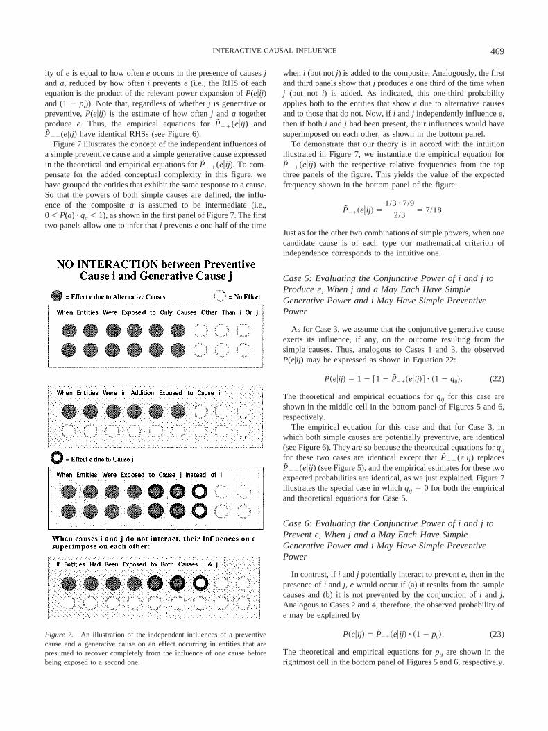
Figure 7 illustrates the concept of the independent influences ofa simple preventive cause and a simple generative cause expressedin the theoretical and empirical equations for P̃�(e�ij). To com-pensate for the added conceptual complexity in this figure, wehave grouped the entities that exhibit the same response to a cause.So that the powers of both simple causes are defined, the influ-ence of the composite a is assumed to be intermediate (i.e.,0 � P(a) � qa � 1), as shown in the first panel of Figure 7. The firsttwo panels allow one to infer that i prevents e one half of the time

when i (but not j) is added to the composite. Analogously, the firstand third panels show that j produces e one third of the time whenj (but not i) is added. As indicated, this one-third probabilityapplies both to the entities that show e due to alternative causesand to those that do not. Now, if i and j independently influence e,then if both i and j had been present, their influences would havesuperimposed on each other, as shown in the bottom panel.

To demonstrate that our theory is in accord with the intuitionillustrated in Figure 7, we instantiate the empirical equation forP̃�(e�ij) with the respective relative frequencies from the topthree panels of the figure. This yields the value of the expectedfrequency shown in the bottom panel of the figure:

P̃��e�ij� �1/3 � 7/9

2/3� 7/18.

Just as for the other two combinations of simple powers, when onecandidate cause is of each type our mathematical criterion ofindependence corresponds to the intuitive one.

Case 5: Evaluating the Conjunctive Power of i and j toProduce e, When j and a May Each Have SimpleGenerative Power and i May Have Simple PreventivePower

As for Case 3, we assume that the conjunctive generative causeexerts its influence, if any, on the outcome resulting from thesimple causes. Thus, analogous to Cases 1 and 3, the observedP(e|ij) may be expressed as shown in Equation 22:

P�e�ij� � 1 � �1 � P̃��e�ij�� 1 � qij�. (22)

The theoretical and empirical equations for qij for this case areshown in the middle cell in the bottom panel of Figures 5 and 6,respectively.

The empirical equation for this case and that for Case 3, inwhich both simple causes are potentially preventive, are identical(see Figure 6). They are so because the theoretical equations for qij

for these two cases are identical except that P̃�(e�ij) replacesP̃��(e�ij) (see Figure 5), and the empirical estimates for these twoexpected probabilities are identical, as we just explained. Figure 7illustrates the special case in which qij 0 for both the empiricaland theoretical equations for Case 5.

Case 6: Evaluating the Conjunctive Power of i and j toPrevent e, When j and a May Each Have SimpleGenerative Power and i May Have Simple PreventivePower

In contrast, if i and j potentially interact to prevent e, then in thepresence of i and j, e would occur if (a) it results from the simplecauses and (b) it is not prevented by the conjunction of i and j.Analogous to Cases 2 and 4, therefore, the observed probability ofe may be explained by

P�e�ij� � P̃��e�ij� � �1 � pij�. (23)

The theoretical and empirical equations for pij are shown in therightmost cell in the bottom panel of Figures 5 and 6, respectively.

Figure 7. An illustration of the independent influences of a preventivecause and a generative cause on an effect occurring in entities that arepresumed to recover completely from the influence of one cause beforebeing exposed to a second one.


The empirical equation for pij in this situation is identical to thatfor Case 4, in which both simple causes are potentially preventive.Analogous to our discussion of Case 5, this identity follows fromthe comparability of the respective theoretical equations (see Fig-ure 5) and the equivalence of the empirical estimates for P̃��(e�ij)and P̃�(e�ij). Therefore, as for Case 4, when i and j do notinteract,

P�e�ij� � P�e��i�j �P�e�i�j � � P�e��ij� � 1,

and pij 0. This special case for the theoretical and empiricalequations for Case 6 is illustrated in Figure 7.

Summary of Our Theory of Conjunctive Causal Power

We have presented an analysis of how a reasoner might assesswhether two candidate causes interact to influence an effect. Ex-tending Cheng’s (1997) theory of simple causes to conjunctivecauses, we propose that reasoners consider �Pij P(e�ij) � P̃(e�ij),the deviation of the observed probability of an effect e given thepresence of both candidate causes i and j from the expectedprobability of e if the two candidates exerted their simple powersonly (Equation 5). To obtain an estimate of the causal power of theconjunction of i and j, reasoners explain each of these two condi-tional probabilities by the simplest possible conception of thecauses of e relevant to that conditional probability (see Table 1).From our set of assumptions, in conjunction with the no-confounding condition, we derived the mathematical results con-cerning the expected probability of e and generative and preven-tive conjunctive power summarized in Figures 5 and 6.

As the column labeled P̃(e|ij) in Figure 6 shows, the empiricalequations for the expected probabilities follow two patterns, onefor situations in which the simple powers of i and j are bothpotentially generative, and the other for those in which the simplepower of at least one candidate is potentially preventive. Theseresults for P̃(e|ij), which are illustrated in Figures 1, 2, and 7, implythat different measures of interactive causal influence are applica-ble depending on the direction of the simple powers.

As the columns labeled qij and pij in Figure 6 show, the empir-ical equations for estimating conjunctive power differ dependingnot only on the direction of the simple powers (compare the threerows) but also on the direction of �Pij.

15 According to our theory,if �Pij � 0, the reasoner evaluates qij, the potential generativepower of the conjunction of i and j. It is estimated by the poten-tially positive difference made by the presence of the conjunctivecandidate to the frequency with which e occurs among entities inwhich e is not already produced by causes other than that candi-date. Analogously, if ‚Pij � 0, the reasoner evaluates pij, theconjunctive candidate’s potential preventive power. It is estimatedby the potentially negative difference made by the presence of theconjunction to the frequency with which e occurs among entities inwhich e is already produced by other causes.

Our results show that conjunctive causal power is analogous tosimple causal power. As illustrated in Figure 5, the equations forqij have a form analogous to Equation 3, the one for simplegenerative power, and the equations for pij have a form analogousto Equation 4, the one for simple preventive power. The conjunc-tive equations differ from their simple power counterparts only

with respect to the expected probability of e on their RHSs. As forsimple power, conjunctive power allows the reasoner to predict therelative frequency with which the candidate cause influences e ina set of entities in the world, independently of how often othercauses in the context might influence e.

Finally, our derivations explain when and why conjunctivecausation can be inferred from covariation, thereby explainingsome basic principles of experimental design as well as reasoners’corresponding everyday intuitions. They explain why no con-founding is a requirement for inferring conjunctive causation, justas Cheng’s (1997, 2000) derivations do for inferring simple cau-sation. Similarly, the theoretical equations (see Figure 5) for con-junctive power explain two other boundary conditions for inferringinteractive causal influence. As we discussed, these equationsmake predictions regarding situations involving the ceiling effectand its preventive analogue that are in accord with both intuitionsand the corresponding principles of experimental design. Thus,these basic principles of design, which are extrinsic to purelycovariational measures and either augment or overrule their inter-pretation, arise from the same assumptions as do the measuresunder our causal approach, and they are intrinsically incorporatedinto these measures.

The Relation Between Our Theory and Other PossibleTheories

In the sense that our theory applies only to candidate causes andeffects of the type specified when the theory’s assumptions hold,it is of course merely a specific model. Other assumptions wouldlead to other models (as we illustrate later with the parallel con-ception of conjunctive causation; see The Assumption That theConjunctive Cause Operates on the Static Outcome of the SimpleCauses). Similarly, causes and effects that are represented by othertypes of variables (e.g., continuous ones) would require othermodels. We think, however, that our theory holds a special placein two senses.

Representation of Distal Causal Relations

Our theory explicitly represents distal conjunctive relationsrather than proximal ones—that is, those that exist in the worldrather than merely in our senses—as the goal of causal discovery,in contrast to all purely covariational models of causation (includ-

15 When �Pi �Pj 0, all three expected probabilities are applicable.The values resulting from the various expected probability equations (andlikewise those resulting from the applicable conjunctive power measures)agree when the simple generative and preventive powers of i and j all equal0. For example, suppose e always occurs when i and j are both present butonly occurs with a probability of .05 otherwise, so that the simple powers(both generative and preventive) of i and j equal 0. In this case, theexpected probabilities (P̃(e|ij), P̃��(e|ij), and P̃�(e|ij)) would all equal.05, and the qijs would all equal 1. The only situation in which the variousexpected probabilities give disagreeing values is when a simple power hasan undefined value. For example, instead of letting P(e|i�j ) P(e|�ij) P(e|�i�j ) .05, let them all be 0 (with P(e|ij) 1 as before). In this case, thesimple generative powers of i and j remain at 0, P̃(e|ij) is 0, and qij is 1.But, the simple preventive powers of i and j are undefined, leadingP̃��(e|ij) and P̃�(e|ij) and their corresponding qijs to also have undefinedvalues, as they should.


ing conventional statistics for categorical data).16 Presumably,distal causal relations remain the goal of causal discovery regard-less of the type of variable representing the causes and effects. Ifso, the same distinction regarding whether distal causal relationsare represented explicitly may lead to similar implications forcausal inference involving other types of variables under other setsof assumptions. (We review evidence in a later section that untu-tored reasoners behave as though they are inferring distal causalrelations; see Empirical Tests of the Conjunctive Power PCTheory.)

Simplicity of Assumptions

We subscribe to the common view in science that parsimony isa virtue. Compared with other models taking the same distalapproach, our assumptions are probably as weak (i.e., general) andas few as they could be to nonetheless allow causal inferenceregarding conjunctive causes when both simple candidates havecausal power. Consider models that infer causal structure withoutinferring causal strength (Pearl, 2000; Spirtes et al., 2000). Al-though such structural models make weaker assumptions thanours, they would be able to identify conjunctive causation onlywhen certain patterns of results are observed. In particular, theywould do so only for cases in which there is a difference in thestate of dependence (i.e., dependent vs. independent) betweeneffect e and the conjunction of candidate causes that (a) would beexpected assuming that the two candidates influence e indepen-dently and (b) is observed. For example, if the constituents of theconjunction are both independent of e, the conjunction would beexpected to be independent of e, and any deviation from indepen-dence between e and the conjunction, which qualitative models canmeasure, would indicate conjunctive causation. When at least onesimple candidate has causal power, however, the same state ofdependence would result whether or not there is causal interaction,unless the conjunctive cause coincidentally exactly cancels theinfluence(s) of the simple cause(s). For the noncoincidental cases,because there would be no difference between the expected and theobserved states even when there is causal interaction, qualitativemodels would be unable to identify conjunctive causation.

Simple models, however, can often be simplistic. We assumethat, in the absence of prior causal knowledge, reasoners wouldconsider more complex models when motivated by evidence con-tradicting a simpler model. For example, they might form hypoth-eses described by Cheng’s (1997) theory of simple power first, butevidence for the violation of the independent-influence assumptionin her theory would lead to the consideration of hypotheses de-scribed by our theory. In turn, the violation of assumptions in ourtheory would lead to the consideration of yet more complexhypotheses.

The role of simplicity in guiding theory development motivatedour assumption, described in conjunction with Case 3, that rea-soners consider the influences of simple and conjunctive causessequentially. This conception is compatible with the view thatreasoners infer a conjunctive cause only after finding that simplecauses alone provide an inadequate explanation. In the next sec-tion, we consider a different conception of the influences of thesimple and conjunctive causes.

Violations of Various Assumptions Underlying theTheory

Our results for P̃(e|ij) are demonstrably true for situations inwhich our assumptions hold. Consider a hypothetical case ofindependent causal influence: Suppose that among the many ap-plicants to a college, 100 are judged to be equally qualified foradmission. The college can unfortunately admit only 50 students.There are two admissions officers, each of whom mistakenlyassumes that he or she is the one making the final decisions, andeach admits 50 on behalf of the college without knowledge of theother’s actions. They are the only admissions officers, so that ifboth of them had been negligent and failed to make any decisions,0 students would have been admitted. Assuming that their criteriafor admission have no related biases (e.g., they each randomlyselect 50), the expected number of students admitted by the collegewould be 75. This answer is congruent with our theory but con-tradicts (a) the interaction contrast from the probabilistic contrastmodel (Cheng & Novick, 1990, 1992), (b) the summation ofassociative strengths in the definition of Rescorla and Wagner’s(1972) model, and (c) the cross-product ratio, all of which predictthat the expected number of students admitted should be 100.

Our assumptions, however, may not hold. In this section, wediscuss some implications of violations of two of these assump-tions: (a) that alternative causes influence e independently of i, j,and their conjunction and (b) that the conjunctive cause operateson the static outcome of the simple causes (i.e., the sequentialconception of simple and conjunctive causal influence). Evenwhen our particular theory is inapplicable because of a violation ofits assumptions, our general approach of representing distal causalrelations may nonetheless be applicable for other sets ofassumptions.

The Assumption That Alternative Causes Influence eIndependently of Candidate Causes i, j, and Their

Conjunction

This assumption and its analogue in Cheng’s (1997) theory ofsimple causal power (namely, that the composite a influences eindependently of i) are probably nearly always violated. A naturalquestion therefore arises: Why should one bother to read workadopting this assumption? For simple causal power, the answer isthat under two conditions, the estimates are nonetheless normative.These conditions are relevant when the assumption of independentinfluence is violated without the reasoner’s knowledge (Cheng,2000), such as when the interacting factor is unobservable. If theviolation involves observable factors only, the reasoner may assessconjunctive power, making the present article rather than Cheng’s(2000) article relevant. These conditions are that (a) the unobserv-able factors that interact with i occur with a similar probabilityacross the learning context and the prediction (i.e., transfer) con-text, and (b) whichever factor or composite of factors in a thatinteracts with i—call it j—does not do so in such a way that i and

16 Bliss (1939) derived the same expected probabilities of e as we did,but we were not acquainted with that work at the time we developed ourtheory. We are not aware of the distal approach being carried through to theconjunctive cause.


the conjunctive cause composed of i and j influence e in oppositedirections (i.e., i is generative but the conjunction of i and j ispreventive, or vice versa). Cheng’s (2000) analysis explains whyin many situations a reasoner is able to make a useful inferenceregarding simple causal power—for example, that striking a matchcauses it to light, or that smoking causes lung cancer—despite theobvious violation of the assumption of the independent influenceof i and a. In those cases, the unobservable enabling conditions(e.g., oxygen for the lighting of the match) occur with a similarprobability across contexts, and they enable rather than disable thegenerative influence of the candidate (i.e., that of striking a matchon lighting).

We have not done a systematic analysis of the implications ofthe violation of the analogous independent-influence assumptionin our conjunctive power theory—an analysis that is muchneeded.17 Nevertheless, let us consider an example of this viola-tion and illustrate it by a modification to Figure 1. Suppose (a) thatthere is some unobservable factor in some of the entities thatmakes them susceptible to cause i and (b) that the same factorprevents them from being susceptible to cause j, in such a way thatthe entities that responded to i in the second panel and those thatresponded to j in the third panel become mutually exclusive. Inthese two panels, because i and j never both occur, they cannotdirectly interact with each other. What this pattern of outcomesreveals instead is that there is some interaction involving each ofi and j individually and some common factor in a, violating ourindependent influence assumption. Even though i and j indirectlyinteract, it is nonetheless possible that they do not directly interact.For example, suppose that the influences of i and j shown in the(modified) middle two panels of Figure 1 superimpose in thebottom panel, so that all nine entities show e in that panel. It seemsto us that the superimposition indubitably indicates that i and j donot directly interact. But, because our theory only uses informationregarding the proportion of entities that show e in each panel (inparticular, it is oblivious to information on the proportion ofentities that show e both in the second panel and in the third), itwill judge that i and j interact to influence e. What then does anindication of interaction or independence according to our mea-sures mean?

One interpretation is that a conclusion of independence resultingfrom our measures implies that i and j do not interact to influencee in any way, directly or indirectly (unless there is some coinci-dental canceling of interactive influences). Independence as indi-cated by our measures is the cleanest possible type of indepen-dence. A conclusion of interaction resulting from our measures,however, does not necessarily imply a direct interaction between iand j, but could also indicate an indirect one via some commonthird factor.

To discern the exact manner in which i interacts with j, moreanalysis would be needed on additional information. If the factorin a that interacts with i and with j is observable, these respectiveinteractions would be assessable by applying our conjunctivepower analysis to them. There is no circularity in that the com-posite a is progressively stripped down. Even if this factor in a isnot observable, however, these interactions are assessable usingour approach, but information of the type in Figure 2 must beavailable. Specifically, there must be information about the pres-ence or absence of each causal candidate and of the effect from arepeated-measures design in which the entities can be reasonably

assumed to recover from exposure to each candidate cause alone.These implications of violating the independent-influence assump-tion in question are not particular to our approach, but pertain toany assessment of interactive causal influence.

The Assumption That the Conjunctive Cause Operates onthe Static Outcome of the Simple Causes

The Sequential (Cure) Conception

In Cases 3 and 5, we assumed that the influence of the conjunc-tive cause on e is not further subjected to the influence of thesimple causes. An everyday example of sequential influenceswould be a medicine curing a disease: The disease (the outcomeproduced by some cause) first occurs, then the medicine cures it.As we mentioned, the ordering of simple and conjunctive influ-ences we have been assuming is consonant with the view thatconjunctive power is assessed only when evidence indicates thatthe explanation in terms of simple powers alone is inadequate.

We believe that the sequential conception is parsimonious andpsychologically plausible; it is probably the default conception.However, it is not the only possible or even reasonable conceptionto consider. In the following section, we briefly discuss an alter-native conception.

The Parallel (Suppressant) Conception18

It is possible that the influences of simple and conjunctivecauses act in parallel. This conception does not alter the explana-tions of P̃(e|ij), as those probabilities do not involve any conjunc-tive causation. The expected probabilities therefore remain asshown in Figures 5 and 6. The explanations of P(e|ij) do change,however, yielding different estimates of conjunctive power in twoof the six cases we considered—when the conjunction may havegenerative power and at least one of the simple causes has pre-ventive power (Cases 3 and 5).

The critical difference lies in the conception of prevention. Inthe parallel conception, prevention acts like a general suppressantrather than a cure. An example would be the current sustained drugregimen for HIV-positive patients, which both blocks the progres-sion of AIDS and relieves the symptoms that have already ap-peared. Because all causes act in parallel, the temporal ordering ofthe occurrence of the candidate causes does not matter.

In the Appendix, we expand the power explanation of P(e|ij)under the two conceptions for Case 3 to explain the exact differ-ence between them. A consequence of the suppressant assumptionis that the upper bound on P(e|ij) is less than 1. Even if thegenerative causes, including the conjunction, succeed in producinge in all entities, only a fraction of these occurrences of e will beprevented by neither i nor j. For Case 3, in which both i and j mayhave simple preventive power, the upper bound is (1 � pi) � (1 �pj). For Case 5, in which i may have simple preventive power andj may have simple generative power, the upper bound is (1 � pi).In contrast, the upper bound on P(e|ij) is always 1 according to thecure conception.

17 We thank Clark Glymour for bringing to our attention various suchimplications.

18 This is the conception cited in Cheng’s (2000) article.


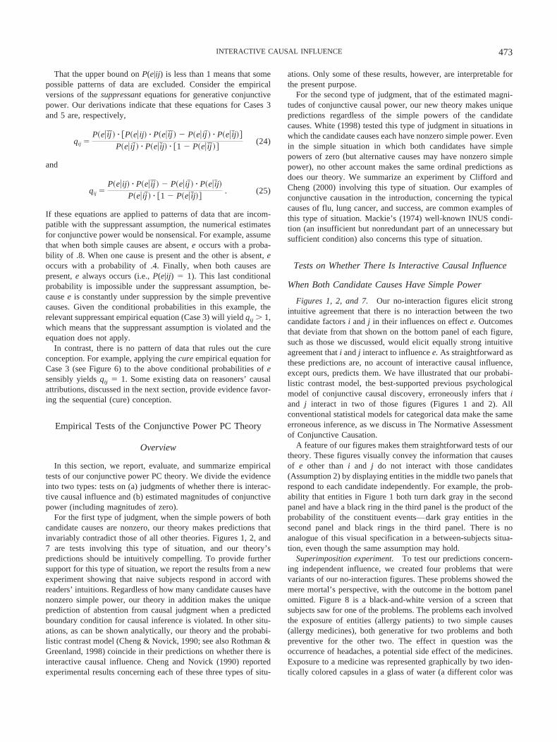
That the upper bound on P(e|ij) is less than 1 means that somepossible patterns of data are excluded. Consider the empiricalversions of the suppressant equations for generative conjunctivepower. Our derivations indicate that these equations for Cases 3and 5 are, respectively,

qij �P�e��i�j � � �P�e�ij� � P�e��i�j � � P�e�i�j � � P�e��ij��

P�e�i�j � � P�e��ij� � �1 � P�e��i�j �� (24)

and

qij �P�e�ij� � P�e��i�j � � P�e�i�j � � P�e��ij�

P�e�i�j � � �1 � P�e��ij�� . (25)

If these equations are applied to patterns of data that are incom-patible with the suppressant assumption, the numerical estimatesfor conjunctive power would be nonsensical. For example, assumethat when both simple causes are absent, e occurs with a proba-bility of .8. When one cause is present and the other is absent, eoccurs with a probability of .4. Finally, when both causes arepresent, e always occurs (i.e., P(e|ij) 1). This last conditionalprobability is impossible under the suppressant assumption, be-cause e is constantly under suppression by the simple preventivecauses. Given the conditional probabilities in this example, therelevant suppressant empirical equation (Case 3) will yield qij � 1,which means that the suppressant assumption is violated and theequation does not apply.

In contrast, there is no pattern of data that rules out the cureconception. For example, applying the cure empirical equation forCase 3 (see Figure 6) to the above conditional probabilities of esensibly yields qij 1. Some existing data on reasoners’ causalattributions, discussed in the next section, provide evidence favor-ing the sequential (cure) conception.

Empirical Tests of the Conjunctive Power PC Theory

Overview

In this section, we report, evaluate, and summarize empiricaltests of our conjunctive power PC theory. We divide the evidenceinto two types: tests on (a) judgments of whether there is interac-tive causal influence and (b) estimated magnitudes of conjunctivepower (including magnitudes of zero).

For the first type of judgment, when the simple powers of bothcandidate causes are nonzero, our theory makes predictions thatinvariably contradict those of all other theories. Figures 1, 2, and7 are tests involving this type of situation, and our theory’spredictions should be intuitively compelling. To provide furthersupport for this type of situation, we report the results from a newexperiment showing that naive subjects respond in accord withreaders’ intuitions. Regardless of how many candidate causes havenonzero simple power, our theory in addition makes the uniqueprediction of abstention from causal judgment when a predictedboundary condition for causal inference is violated. In other situ-ations, as can be shown analytically, our theory and the probabi-listic contrast model (Cheng & Novick, 1990; see also Rothman &Greenland, 1998) coincide in their predictions on whether there isinteractive causal influence. Cheng and Novick (1990) reportedexperimental results concerning each of these three types of situ-

ations. Only some of these results, however, are interpretable forthe present purpose.

For the second type of judgment, that of the estimated magni-tudes of conjunctive causal power, our new theory makes uniquepredictions regardless of the simple powers of the candidatecauses. White (1998) tested this type of judgment in situations inwhich the candidate causes each have nonzero simple power. Evenin the simple situation in which both candidates have simplepowers of zero (but alternative causes may have nonzero simplepower), no other account makes the same ordinal predictions asdoes our theory. We summarize an experiment by Clifford andCheng (2000) involving this type of situation. Our examples ofconjunctive causation in the introduction, concerning the typicalcauses of flu, lung cancer, and success, are common examples ofthis type of situation. Mackie’s (1974) well-known INUS condi-tion (an insufficient but nonredundant part of an unnecessary butsufficient condition) also concerns this type of situation.

Tests on Whether There Is Interactive Causal Influence

When Both Candidate Causes Have Simple Power

Figures 1, 2, and 7. Our no-interaction figures elicit strongintuitive agreement that there is no interaction between the twocandidate factors i and j in their influences on effect e. Outcomesthat deviate from that shown on the bottom panel of each figure,such as those we discussed, would elicit equally strong intuitiveagreement that i and j interact to influence e. As straightforward asthese predictions are, no account of interactive causal influence,except ours, predicts them. We have illustrated that our probabi-listic contrast model, the best-supported previous psychologicalmodel of conjunctive causal discovery, erroneously infers that iand j interact in two of those figures (Figures 1 and 2). Allconventional statistical models for categorical data make the sameerroneous inference, as we discuss in The Normative Assessmentof Conjunctive Causation.

A feature of our figures makes them straightforward tests of ourtheory. These figures visually convey the information that causesof e other than i and j do not interact with those candidates(Assumption 2) by displaying entities in the middle two panels thatrespond to each candidate independently. For example, the prob-ability that entities in Figure 1 both turn dark gray in the secondpanel and have a black ring in the third panel is the product of theprobability of the constituent events—dark gray entities in thesecond panel and black rings in the third panel. There is noanalogue of this visual specification in a between-subjects situa-tion, even though the same assumption may hold.

Superimposition experiment. To test our predictions concern-ing independent influence, we created four problems that werevariants of our no-interaction figures. These problems showed themere mortal’s perspective, with the outcome in the bottom panelomitted. Figure 8 is a black-and-white version of a screen thatsubjects saw for one of the problems. The problems each involvedthe exposure of entities (allergy patients) to two simple causes(allergy medicines), both generative for two problems and bothpreventive for the other two. The effect in question was theoccurrence of headaches, a potential side effect of the medicines.Exposure to a medicine was represented graphically by two iden-tically colored capsules in a glass of water (a different color was


used for each medicine). Nonexposure to the medicines was rep-resented by a glass without the capsules.

For both preventive problems, the first panel showed that allallergy patients had headaches when they received neither medi-cine. One problem, which presented outcomes for 9 patients, wasa direct analogue of Figure 2: Every dark gray circle in that figurewas replaced by a frowning face, indicating headache, and everylight gray ring in that figure was replaced by a happy face,indicating no headache. The drugs therefore respectively preventedheadaches for two thirds and one third of the patients. In the otherproblem, in which there were 12 patients, the second and thirdpanels each showed that 6 patients had headaches, with 3 havingheadaches in both panels, as would be expected if the patientsresponded to the two drugs independently. The drugs thereforeeach prevented headaches for one half of the patients. The twogenerative problems were exact analogues of the preventive prob-lems, with values of the outcome (headache and no headache)reversed throughout. For example, the first panel showed thatnone, rather than all, of the patients had headaches when theyreceived neither medicine (see Figure 8). The drugs in theseproblems therefore caused headaches with the same probabilitiesas their preventive counterparts prevented them.

Forty undergraduate students enrolled in an introductory psy-chology class at University of California, Los Angeles, were

randomly assigned to receive one of the four problems (n 10 foreach problem). The four panels for a problem were presentedsequentially and cumulatively on a computer screen until all panelsappeared (as in Figure 8). (There was an added screen interveningbetween the presentation of the middle two panels, which showeda panel depicting the complete recovery of the patients from thefirst medicine to their original state before the second medicinewas given [not shown in Figure 8].) The subjects were asked aboutthe influence of each medicine on headaches as the informationwas presented.

The fourth panel, which concerned the hypothetical situation inwhich both medicines had been given, depicted faces covered withquestion marks (see Figure 8). Subjects were then asked a series ofquestions that tested the novel predictions of our theory. First, theywere asked, “Assuming that nothing unexpected happened, howmany [of the patients in this panel] would have had a headache?”To answer this question, subjects first indicated whether more orfewer patients would have had a headache in the bottom panel thanin either of the two middle panels, and then they explained theiranswer. The response options were “more,” “fewer,” and either“neither” (for the problems with 9 patients and unequal simplepowers) or “just as many” (for the problems with 12 entities andequal simple powers). We included this qualitative question todiscourage subjects from doing arithmetic mechanically withoutthinking about causality. All but 2 of the 40 subjects gave answersto this question that were consistent with our theory. (The 2subjects whose answers were inconsistent with our theory receivedthe preventive problem with 9 entities.)

Then came the critical question—“What is the most likelynumber of patients who would have had a headache in the bottompanel?”—followed by a blank. The predictions of our theory are asfollows: (a) 9 for the generative problem with 12 entities (seeFigure 8), (b) 7 for the generative problem with 9 entities (seeFigure 1), (c) 3 for the preventive problem with 12 entities, and (d)2 for the preventive problem with 9 entities (see Figure 2). Col-lapsed across the four problems, the vast majority of subjects (37of 40) gave the answer predicted by our theory. Only 1 subject(who received the generative problem with 9 entities) gave theanswer predicted by our old probabilistic contrast model (Cheng &Novick, 1990, 1992), the Rescorla–Wagner (1972) model, and thecross-product ratio (i.e., all patients have a headache for the twogenerative problems and no patients have a headache for the twopreventive problems). The other 2 subjects gave other answerswith incoherent justifications (these were the same subjects whogave nonconforming answers to the previous question).

For further confirmation of their most preferred response, sub-jects were next shown two patterns of possible results for thebottom panel (with the order of presentation counterbalanced) andwere asked to indicate the pattern with which they agreed. Onepattern corresponded to the prediction of our theory (analogous tothe bottom panels in Figures 1 and 2); the other corresponded tothe prediction of the other models (Cheng & Novick, 1990, 1992;Rescorla & Wagner, 1972; and the cross-product ratio). For thisquestion, 39 of the 40 subjects picked the pattern predicted by ourtheory to indicate independent influence. The lone exception wasthe subject whose numeric response to the previous questionmatched the alternative pattern.

Finally, subjects were asked whether the pattern they had justselected is the best possible answer to the question of what would

Figure 8. A black-and-white version of the information provided for oneproblem in which subjects were asked to predict the data pattern that wouldindicate the independent influence of candidates i and j when they arejointly present.


have happened if both medicines had been given at the same time.For this question, 37 subjects gave an answer consistent with ourtheory: 34 indicated that the pattern predicted by our theory wasthe best possible answer, and 3 indicated that it was not necessarilythe best because the drugs might interact (note that these subjectsspontaneously explained a deviation in terms of an interaction).Only 1 subject said that the other pattern was the best possibleanswer (the subject who spontaneously predicted that pattern).Clearly, the results of this experiment strongly favor our theoryover other accounts.

Cheng and Novick (1990). In their experiment, Cheng andNovick (1990) tested a set of inference problems (Problems 10, 11,and 12) in which two candidate causes each had a simple gener-ative power of 1: The effect in question never occurred when bothcandidates were absent but always occurred when either candidatewas present without the other. In addition, the effect alwaysoccurred in the joint presence of the two causes. Thus, the inter-action contrast for these factors from the probabilistic contrastmodel (Equation 2) has a value of �1, implying preventive inter-active influence. In contrast, according to our conjunctive powerPC theory, �P 0, implying that subjects should not indicatethat this conjunction is a cause. In fact, most subjects did not.Unfortunately, this result is ambiguous: The conjunctive causepredicted by the probabilistic contrast model is preventive, and ourresponse format did not distinguish between generative and pre-ventive causes. As we elaborate in the next section, subjects weresimply asked to explain a target event by choosing from a givenlist of response categories. Because a preventive cause cannotexplain the occurrence of the effect in question in the target event,subjects might have omitted the relevant response category despitetheir perception of preventive efficacy.

When Only One Candidate Cause Has Simple Power

Overview of Cheng and Novick (1990). Subjects were givenshort scenarios describing the occurrence of a certain effect overvarious values of people, stimuli, and occasions (the candidatecausal dimensions). To ensure that their responses reflected infer-ences based on the experimental materials rather than on knowl-edge retrieved from memory, the problems involved fictionalevents that were said to occur in an imaginary land where people’scustoms and preferences often differed from our own. For exam-ple, one problem (Number 3) was as follows (Cheng & Novick,1990, p. 565):

Adam thinks that narcissus (a flower) smells nice on this occasion.

1. In fact, Adam has always thought that narcissus smells nice.

2. But nobody else has ever thought that narcissus smells nice.

3. Everyone has always thought that all other flowers smell nice.

On the basis of such information, subjects were asked to explainwhat caused the italicized target event by choosing one or moreresponses from a list of seven given beneath the problem. The firstthree responses corresponded to the three possible simple causes:the target person, stimulus, and occasion, respectively. For exam-ple, the stimulus attribution for the narcissus problem was “there issomething special about narcissus in general.” The next three

responses corresponded to the three possible conjunctive causesinvolving combinations of two of the three factors. For example,the Person � Stimulus interaction attribution was presented as“there is something special about the combination of Adam andnarcissus (only when they are together).” The final response cor-responded to the three-way interaction.

Note that the variables in the stimuli were not binary. Therefore,our new theory applies only if the stimuli were recoded as binaryby subjects, for example, to represent that there is somethingspecial about the target person that is absent in other people. Thatsuch recoding occurred is not implausible given the wording of theresponse categories and the references to the nontarget values oneach dimension in the aggregate (e.g., nobody, everyone, always,all other).

Cheng and Novick’s (1990) materials consisted of various setsof three problems in which the problems within each set werelogically equivalent; they were merely the three possible rotationsof the same logical structure in the Person � Stimulus � Occasionspace. They were so designed to test a possible bias for perceivingthe person dimension as causal more often than other dimensions(i.e., the fundamental attribution error; see Nisbett & Ross, 1980).For our purpose here, the problems in each set were simplyreplications instantiated with different stimulus materials con-ducted on different groups of subjects. There were four sets ofproblems for which the probabilistic contrast model, our conjunc-tive power PC theory, or both, predict a two-way interactionattribution (e.g., the conjunction of Adam and narcissus in theexample). We considered one of these sets in the previous section.Of the remaining three, only two have results that shed light on ournew theory. We consider these two sets in detail here.

Results. For the situation in which only one candidate causehas nonzero simple power, our new theory and our old modelconcur in their predictions regarding whether there is a conjunctivecause when no boundary condition for that inference is violated.Two sets of problems (one consisting of Problems 2, 5, and8—N 66 for the set; the other consisting of Problems 3, 6, and9—N 72 for the set) tested in Cheng and Novick’s (1990) studyconcerned this situation. These problems had probabilistic con-trasts that yielded predicted causal attributions corresponding tothe six possible combinations of (a) a conjunctive cause consistingof two factors (e.g., Person � Stimulus) and (b) a simple causeconsisting of one of the constituents of the conjunction (Person orStimulus for the example). It is interesting to note that for theseproblems, a boundary condition for inferring conjunctive causationwas violated according to the parallel (suppressant) conception ofconjunctive causation but not the sequential (cure) conception, theone that we favor as a default.

The pattern of covariation was as shown in Figure 9. None of theaccounts under consideration predicts more than one conjunctivecause; we therefore label the factors composing the predictedconjunctive cause i and j here for expository purposes. This patternindicates that the simple preventive power of i (narcissus in theexample) is 1, and the simple preventive powers of j (Adam) andk (this occasion) are 0. Collapsing across k, the interaction contrastfor i and j from the probabilistic contrast model (Equation 2) hasa value of 1, predicting that the conjunction of those factors (Adam& narcissus) is a generative cause. Likewise, according to thesequential (cure) conception of the conjunctive power PC theory,�P� and �P�� each equals 1, implying that qij 1. Thus, these


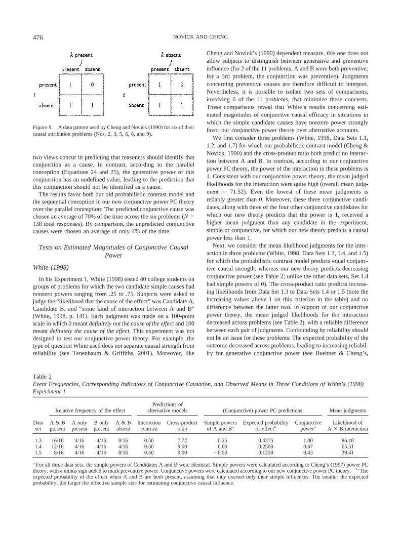
two views concur in predicting that reasoners should identify thatconjunction as a cause. In contrast, according to the parallelconception (Equations 24 and 25), the generative power of thisconjunction has an undefined value, leading to the prediction thatthis conjunction should not be identified as a cause.

The results favor both our old probabilistic contrast model andthe sequential conception in our new conjunctive power PC theoryover the parallel conception: The predicted conjunctive cause waschosen an average of 70% of the time across the six problems (N 138 total responses). By comparison, the unpredicted conjunctivecauses were chosen an average of only 4% of the time.

Tests on Estimated Magnitudes of Conjunctive CausalPower

White (1998)

In his Experiment 1, White (1998) tested 40 college students ongroups of problems for which the two candidate simple causes hadnonzero powers ranging from .25 to .75. Subjects were asked tojudge the “likelihood that the cause of the effect” was Candidate A,Candidate B, and “some kind of interaction between A and B”(White, 1998, p. 141). Each judgment was made on a 100-pointscale in which 0 meant definitely not the cause of the effect and 100meant definitely the cause of the effect. This experiment was notdesigned to test our conjunctive power theory. For example, thetype of question White used does not separate causal strength fromreliability (see Tenenbaum & Griffiths, 2001). Moreover, like

Cheng and Novick’s (1990) dependent measure, this one does notallow subjects to distinguish between generative and preventiveinfluence (for 2 of the 11 problems, A and B were both preventive;for a 3rd problem, the conjunction was preventive). Judgmentsconcerning preventive causes are therefore difficult to interpret.Nevertheless, it is possible to isolate two sets of comparisons,involving 6 of the 11 problems, that minimize these concerns.These comparisons reveal that White’s results concerning esti-mated magnitudes of conjunctive causal efficacy in situations inwhich the simple candidate causes have nonzero power stronglyfavor our conjunctive power theory over alternative accounts.

We first consider three problems (White, 1998, Data Sets 1.1,1.2, and 1.7) for which our probabilistic contrast model (Cheng &Novick, 1990) and the cross-product ratio both predict no interac-tion between A and B. In contrast, according to our conjunctivepower PC theory, the power of the interaction in these problems is1. Consistent with our conjunctive power theory, the mean judgedlikelihoods for the interaction were quite high (overall mean judg-ment 71.52). Even the lowest of these mean judgments isreliably greater than 0. Moreover, these three conjunctive candi-dates, along with three of the four other conjunctive candidates forwhich our new theory predicts that the power is 1, received ahigher mean judgment than any candidate in the experiment,simple or conjunctive, for which our new theory predicts a causalpower less than 1.

Next, we consider the mean likelihood judgments for the inter-action in three problems (White, 1998, Data Sets 1.3, 1.4, and 1.5)for which the probabilistic contrast model predicts equal conjunc-tive causal strength, whereas our new theory predicts decreasingconjunctive power (see Table 2; unlike the other data sets, Set 1.4had simple powers of 0). The cross-product ratio predicts increas-ing likelihoods from Data Set 1.3 to Data Sets 1.4 or 1.5 (note theincreasing values above 1 on this criterion in the table) and nodifference between the latter two. In support of our conjunctivepower theory, the mean judged likelihoods for the interactiondecreased across problems (see Table 2), with a reliable differencebetween each pair of judgments. Confounding by reliability shouldnot be an issue for these problems: The expected probability of theoutcome decreased across problems, leading to increasing reliabil-ity for generative conjunctive power (see Buehner & Cheng’s,

Figure 9. A data pattern used by Cheng and Novick (1990) for six of theircausal attribution problems (Nos. 2, 3, 5, 6, 8, and 9).

Table 2Event Frequencies, Corresponding Indicators of Conjunctive Causation, and Observed Means in Three Conditions of White’s (1998)Experiment 1

Dataset

Relative frequency of the effectPredictions of

alternative models (Conjunctive) power PC predictions Mean judgments

A & Bpresent

A onlypresent

B onlypresent

A & Babsent

Interactioncontrast

Cross-productratio

Simple powersof A and Ba

Expected probabilityof effectb

Conjunctivepowera

Likelihood ofA � B interaction

1.3 16/16 4/16 4/16 0/16 0.50 7.72 0.25 0.4375 1.00 86.181.4 12/16 4/16 4/16 4/16 0.50 9.00 0.00 0.2500 0.67 65.511.5 8/16 4/16 4/16 8/16 0.50 9.00 �0.50 0.1250 0.43 39.41

a For all three data sets, the simple powers of Candidates A and B were identical. Simple powers were calculated according to Cheng’s (1997) power PCtheory, with a minus sign added to mark preventive power. Conjunctive powers were calculated according to our new conjunctive power PC theory. b Theexpected probability of the effect when A and B are both present, assuming that they exerted only their simple influences. The smaller the expectedprobability, the larger the effective sample size for estimating conjunctive causal influence.


1997, explanation of variations in effective sample size, even whenthe actual sample sizes do not vary).19

White’s (1998) results allow another type of evaluation of ourold and new accounts of conjunctive causal influence. Recall thatour conjunctive power theory, unlike our probabilistic contrastmodel, allows comparison between estimates of causal strength forsimple and conjunctive causes. Seven of White’s problems (DataSets 1.1, 1.2, 1.3, 1.6, 1.7, 1.10, and 1.11) had a conjunctivegenerative power of 1.0 but simple powers ranging from .25 to .75.In support of our causal-power approach, for each of these prob-lems, the observed judged likelihood of the interaction was higherthan the judgments for the two simple candidate causes (the overallmean judged likelihood for the conjunction was 74.35, comparedwith 39.49 for the 14 simple causes).

Clifford and Cheng (2000)

Overview. We now turn to the results of an experiment mea-suring estimated magnitudes of conjunctive power. Clifford andCheng (2000) tested some such predictions of our conjunctivecausal-power theory against those made by the most viable purelycovariational accounts.20 Their experiment concerned a simplesituation involving conjunctive causation: Two candidate causes ofan effect e, labeled i and j for the purpose of exposition here, haveno simple causal power but may (or may not) in combinationinfluence (i.e., generate or prevent) e. The base rate of e (i.e., theprobability of e in the absence of the conjunctive candidate) variedacross problems; because the component factors had no simplepower, there was a single base rate of e within a problem (when-ever i and j were not both present, e occurred with the sameprobability, determined by how often alternative causes producede). The candidates having no simple power implies that they hadno simple preventive power, a condition for distinguishing thesequential and parallel conceptions of conjunctive causation; theresults of this study therefore do not distinguish between theseconceptions, but instead test what is common to them againstalternative accounts.

In this situation, Cheng and Novick’s (1990, 1992) interactioncontrast model reduces to the classical �P model (Jenkins & Ward,1965; see Equation 1), with the modification that the conjunctionof i and j is treated as a single elemental unit—whenever i and j arenot both present, the candidate (i.e., the conjunction of i and j) isconsidered absent. Rescorla and Wagner’s (1972) model may bemodified analogously to treat the conjunction as a single elementalunit (see Clifford & Cheng, 2000). The predictions of that modelregarding elemental units would therefore apply to theconjunction.

To test these accounts, Clifford and Cheng (2000) comparedsubjects’ estimates of conjunctive causal strength across meaning-ful subsets of problems. One set of comparisons involved conjunc-tive candidates that had identical positive, negative, or zero �Pij

(or simple �P for the conjunction; the two contrasts are equivalenthere), but varied with respect to the base rate of e. Our conjunctivecausal-power theory, like Cheng’s (1997) theory of simple causalpower, predicts that with an increase in the base rate of e, estimatesof the causal strength of such conjunctive candidates with the same�Pij will increase when �Pij is positive, decrease when �Pij isnegative, and remain at zero when �Pij is zero (see equations inFigure 5). A second set of comparisons involved candidates with

the same conjunctive power but varying values of �Pij. Our theorypredicts that causal estimates for such candidates will not differ.No purely covariational theory predicts either pattern of results.These divergent predictions reflect the key difference between thetwo approaches in what is assumed to be invariant across contexts:the (unobservable) distal causal relation in the derivation of ourconjunctive power measures versus the (observable) proximal as-sociation in all purely covariational models.

Design. There were 10 within-subject conditions, correspond-ing to 10 conjunctive candidates that varied in their power and �Pij

(see Table 3, first four columns). Each condition (i.e., each causalinference problem) involved a different combination of two can-didate factors (medicines). The conditions that involved generativeconjunctive candidates and those that involved preventive oneswere mirror images of each other. Some pairs of conditions variedthe base rate of e for conjunctive candidates with the same level of�Pij, yielding different conjunctive powers across conditions when�Pij was nonzero (GH vs. CD and MN vs. IJ) but no such changein conjunctive power when �Pij was zero (OP vs. QR). Other pairsvaried �Pij for conjunctive candidates with the same causal power(CD vs. EF and IJ vs. KL). Finally, there were two pairs ofcandidates for which �Pij and conjunctive power predict differ-ences in opposite directions (EF vs. AB and KL vs. ST).

The differential predictions made by our theory and the �Pmodel (Jenkins & Ward, 1965) or interaction contrasts (Cheng &Novick, 1990) should be clear from Table 3. Rescorla and Wag-ner’s (1972) model makes the same predictions as does the �Pmodel if its learning parameter, �, is restricted to remain constantin the presence of e (the unconditioned stimulus in its terminology)and in its absence (Chapman & Robbins, 1990; Cheng, 1997).Without this restriction, as long as the ordering of the values of �is consistent (e.g., �US � �US for all data points in a condition),this model predicts that the base rate of e should influence causalstrength in the same direction for candidates with an equal positive�Pij and for those with an equal negative �Pij (e.g., see Danks,2003; Wasserman, Elek, Chatlosh, & Baker, 1993). Specifically,the (absolute) magnitudes of the judged causal strengths will besmaller as the base rate of e increases for any fixed positive ornegative �Pij if �US � �US but larger if �US � �US.

The cross-product ratio predicts the same ordinal pattern ofcausal judgments as does �P or interaction contrast except forconditions CD and IJ (see the fifth column in Table 3). A value of1 on this criterion indicates no interaction. Increasingly largevalues above 1 indicate increasingly strong generative causes,whereas increasingly small values below 1 indicate increasinglystrong preventive causes. CD is a critical medicine combination forwhich �P predicts the same low value as for GH, whereas con-

19 There were some groups of problems for which the conjunctive powerwas equally 1, but the judged likelihoods were observed to reliably differ.All such differences, however, concerned cases in which there was acorresponding difference in reliability, due to differences in the effectivesample size for estimating the expected probability of the outcome or in theactual sample size for estimating the observed probability of the outcome.The ambiguity of the response scale is likely to have exacerbated theconfounding by variation in reliability.

20 We thank Deborah Clifford for her helpful comments on our accountof this experiment.


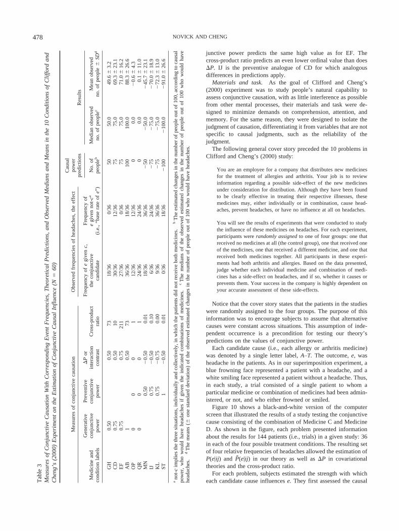
junctive power predicts the same high value as for EF. Thecross-product ratio predicts an even lower ordinal value than does�P. IJ is the preventive analogue of CD for which analogousdifferences in predictions apply.

Materials and task. As the goal of Clifford and Cheng’s(2000) experiment was to study people’s natural capability toassess conjunctive causation, with as little interference as possiblefrom other mental processes, their materials and task were de-signed to minimize demands on comprehension, attention, andmemory. For the same reason, they were designed to isolate thejudgment of causation, differentiating it from variables that are notspecific to causal judgments, such as the reliability of thejudgment.

The following general cover story preceded the 10 problems inClifford and Cheng’s (2000) study:

You are an employee for a company that distributes new medicinesfor the treatment of allergies and arthritis. Your job is to reviewinformation regarding a possible side-effect of the new medicinesunder consideration for distribution. Although they have been foundto be clearly effective in treating their respective illnesses, thesemedicines may, either individually or in combination, cause head-aches, prevent headaches, or have no influence at all on headaches.

You will see the results of experiments that were conducted to studythe influence of these medicines on headaches. For each experiment,participants were randomly assigned to one of four groups: one thatreceived no medicines at all (the control group), one that received oneof the medicines, one that received a different medicine, and one thatreceived both medicines together. All participants in these experi-ments had both arthritis and allergies. Based on the data presented,judge whether each individual medicine and combination of medi-cines has a side-effect on headaches, and if so, whether it causes orprevents them. Your success in the company is highly dependent onyour accurate assessment of these side-effects.

Notice that the cover story states that the patients in the studieswere randomly assigned to the four groups. The purpose of thisinformation was to encourage subjects to assume that alternativecauses were constant across situations. This assumption of inde-pendent occurrence is a precondition for testing our theory’spredictions on the values of conjunctive power.

Each candidate cause (i.e., each allergy or arthritis medicine)was denoted by a single letter label, A–T. The outcome, e, washeadache in the patients. As in our superimposition experiment, ablue frowning face represented a patient with a headache, and awhite smiling face represented a patient without a headache. Thus,in each study, a trial consisted of a single patient to whom aparticular medicine or combination of medicines had been admin-istered, or not, and who either frowned or smiled.

Figure 10 shows a black-and-white version of the computerscreen that illustrated the results of a study testing the conjunctivecause consisting of the combination of Medicine C and MedicineD. As shown in the figure, each problem presented informationabout the results for 144 patients (i.e., trials) in a given study: 36in each of the four possible treatment conditions. The resulting setof four relative frequencies of headaches allowed the estimation ofP(e|ij) and P̃(e|ij) in our theory as well as �P in covariationaltheories and the cross-product ratio.

For each problem, subjects estimated the strength with whicheach candidate cause influences e. They first assessed the causalT

able

3M

easu

res

ofC

onju

ncti

veC

ausa

tion

Wit

hC

orre

spon

ding

Eve

ntF

requ

enci

es,

The

oret

ical

Pre

dict

ions

,an

dO

bser

ved

Med

ians

and

Mea

nsin

the

10C

ondi

tion

sof

Cli

ffor

dan

dC

heng

’s(2

000)

Exp

erim

ent

onth

eE

stim

atio

nof

Con

junc

tive

Cau

sal

Infl

uenc

e(N

60

)

Mea

sure

sof

conj

unct

ive

caus

atio

nO

bser

ved

freq

uenc

ies

ofhe

adac

hes,

the

effe

ctC

ausa

lpo

wer

pred

ictio

nsR

esul

ts

Med

icin

ean

dco

nditi

onla

bels

Gen

erat

ive

conj

unct

ive

pow

er

Prev

entiv

eco

njun

ctiv

epo

wer

�P

orin

tera

ctio

nco

ntra

stC

ross

-pro

duct

ratio

Freq

uenc

yof

egi

ven

c,th

eco

njun

ctiv

eca

ndid

ate

Freq

uenc

yof

egi

ven

not-

ca

(i.e

.,“b

ase

rate

ofe”

)N

o.of

peop

leb

Med

ian

obse

rved

no.

ofpe

ople

cM

ean

obse

rved

no.

ofpe

ople

SD

d

GH

0.50

0.50

7318

/36

0/36

5050

.049

.6

3.2

CD

0.75

0.50

1030

/36

12/3

675

75.0

69.3

23

.1E

F0.

750.

7521

127

/36

0/36

7575

.071

.0

16.2

AB

10.

5073

36/3

618

/36

100

100.

088

.3

26.6

OP

00

01

12/3

612

/36

00.

0�

0.6

4.

3Q

R0

00

124

/36

24/3

60

0.0

0.1

11

.0M

N0.

50�

0.50

0.01

18/3

636

/36

�50

�50

.0�

45.7

23

.1IJ

0.75

�0.

500.

106/

3624

/36

�75

�75

.0�

70.0

18

.9K

L0.

75�

0.75

0.00

9/36

36/3

6�

75�

75.0

�72

.3

13.0

ST1

�0.

500.

010/

3618

/36

�10

0�

100.

0�

91.0

26

.6

ano

t-c

impl

ies

the

thre

esi

tuat

ions

,ind

ivid

ually

and

colle

ctiv

ely,

inw

hich

the

patie

nts

did

notr

ecei

vebo

thm

edic

ines

.b

The

estim

ated

chan

ges

inth

enu

mbe

rof

peop

leou

tof

100,

acco

rdin

gto

caus

alpo

wer

,w

how

ould

have

head

ache

sif

give

nth

ein

dica

ted

com

bina

tions

ofm

edic

ines

.c

The

med

ians

ofth

eob

serv

edes

timat

edch

ange

sin

the

num

ber

ofpe

ople

out

of10

0w

how

ould

have

head

ache

s.d

The

mea

ns(

one

stan

dard

devi

atio

n)of

the

obse

rved

estim

ated

chan

ges

inth

enu

mbe

rof

peop

leou

tof

100

who

wou

ldha

vehe

adac

hes.


strengths of the individual medicines (“What effect does Medicine[x] alone have on headaches?”), then that of their conjunction(“What effect do Medicines [x and y] in combination have onheadaches?”). Causal strength was measured in two steps: (a) aqualitative assessment of whether a candidate cause (each medi-cine individually or the two in combination) has any influence one and (b) if the candidate was judged to have an influence, anassessment of the direction of the influence and an estimate of itsextent, as indicated by the frequency of the outcome under acounterfactual intervention on entities that did not show that out-come. In particular, subjects were asked how many patients out of100, all of whom did not show an outcome, would now have theoutcome if the candidate cause were introduced. For example,when subjects indicated that a candidate caused headaches, theywere asked to estimate the number of patients who would get aheadache if the candidate were given to 100 patients withoutheadaches.

The counterfactual questions removed alternative influences ofe of like kind as the candidate (generative or preventive), therebyallowing the influence of the candidate to manifest itself withoutcontamination. They also required subjects to generalize from thelearning to the test context, thereby allowing the measurement ofwhat subjects assumed to be invariant across contexts—either theproximal relation or the distal one.

Using frequency as the dependent measure increases the con-creteness of the reasoning task and therefore would likely improveaccuracy (Tversky & Kahneman, 1983). In particular, it may beless natural to conflate reliability and causal strength when thelatter is indicated by a specific number of discrete entities amonga set of such entities in the world, rather than by a subjective ratingon a scale, as has been typical in previous psychological studies ofcausal induction.

To encourage a uniform interpretation of the values on thedependent measure, Clifford and Cheng (2000) exposed all sub-jects at the outset to three conjunctive candidate causes that shouldyield a wide range of answers on the dependent measure (Parducci,1965): The first three problems illustrated a generative cause, apreventive cause, and a noncausal candidate. For one group ofsubjects, the first three problems were GH, ST, and OP; for asecond group, they were MN, AB, and QR. The other sevenproblems for each group were presented in a different randomorder for each subject.

Results. If subjects (N 60) answered that a medicine “has noeffect” on headaches, their judged causal strength was scored aszero. If they answered that a medicine “causes” headaches, theirnumerical estimate in response to the counterfactual question wasscored verbatim as a positive number; and, if they answered that amedicine “prevents” headaches, their numerical estimate wasscored as a negative number. As expected, all the individualmedicines were judged to be noncausal by virtually all subjects.

The results for the conjunctive candidates are summarized inTable 3. The table lists medians in addition to means, because thedistributions of estimates for most of the conditions were clearlyskewed. The results strongly support the predictions of our con-junctive power theory over those of the probabilistic contrastmodel (Cheng & Novick, 1990) and the cross-product ratio.

We consider first the comparison of the predictions of theconjunctive power PC theory and the probabilistic contrast model.With an increasing base rate of e, the absolute values of theaverage causal judgments for problems with the same level of �Pij

increased when �Pij was positive (compare condition GH with CDand condition CD with AB) and decreased when �Pij was negative(compare condition ST with IJ and condition IJ with MN). More-over, when causal power and �Pij predict differences in oppositedirections (conditions AB and EF and conditions ST and KL), theaverage causal estimates differed in the direction predicted bycausal power. These observed differences, which were all highlyreliable, indicate that subjects’ estimates of causal strength re-flected conjunctive causal power.

In contrast, causal judgments remained at or near zero when�Pij was zero and did not differ reliably across those two condi-tions (OP and QR), despite a variation in the base rate of e.Likewise, when candidates shared the same causal power butvaried in �Pij (generative conditions CD and EF and preventiveconditions IJ and KL), the average causal estimates were nearlyidentical, indicating that estimates of causal strength were not afunction of �Pij.

Next, we consider how the predictions of the cross-product ratiofared. As we noted earlier, this criterion and the �P model differin their predictions for only 2 of the 10 conditions. For theseconditions, the observed judgments deviated even more from thepredictions of the cross-product ratio than from those of theprobabilistic contrast model. For example, CD was observed to

Figure 10. A black-and-white version of the stimulus materials froma condition in Clifford and Cheng’s (2000) study. The figure depictsthe results of a study testing the influences of Medicines C and D onheadaches.


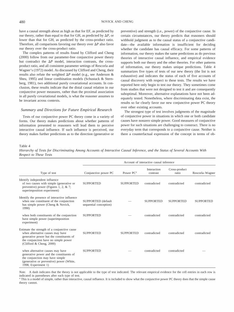
have a causal strength about as high as that for EF, as predicted byour theory, rather than equal to that for GH, as predicted by �P, orlower than that for GH, as predicted by the cross-product ratio.Therefore, all comparisons favoring our theory over �P also favorour theory over the cross-product ratio.

The complex patterns of results found by Clifford and Cheng(2000) follow from our parameter-free conjunctive power theorybut contradict the �P model, interaction contrasts, the cross-product ratio, and all consistent parameter settings of Rescorla andWagner’s (1972) model. As discussed by Clifford and Cheng, theirresults also refute the weighted �P model (e.g., see Anderson &Sheu, 1995) and linear combination models (Schustack & Stern-berg, 1981), two additional purely covariational accounts. In con-clusion, these results indicate that the distal causal relation in ourconjunctive power measures, rather than the proximal associationin all purely covariational models, is what the reasoner assumes tobe invariant across contexts.

Summary and Directions for Future Empirical Research

Tests of our conjunctive power PC theory come in a variety offorms. Our theory makes predictions about whether patterns ofinformation presented to reasoners will lead them to perceiveinteractive causal influence. If such influence is perceived, ourtheory makes further predictions as to the direction (generative or

preventive) and strength (i.e., power) of the conjunctive cause. Incertain circumstances, our theory predicts that reasoners shouldwithhold judgment as to the causal status of a conjunctive candi-date—the available information is insufficient for decidingwhether the candidate has causal efficacy. For some patterns ofinformation, our theory makes the same predictions as do previoustheories of interactive causal influence, and empirical evidencesupports both our theory and the other theories. For other patternsof information, our theory makes unique predictions. Table 4summarizes five types of tests of our new theory (the list is notexhaustive) and indicates the status of each of five accounts ofcausal discovery with respect to these tests. The results we havereported here only begin to test our theory. They sometimes comefrom studies that were not designed to test it and are consequentlysuboptimal. Moreover, alternative explanations have not been ad-equately tested. Nonetheless, where discriminating data exist, theresults so far clearly favor our new conjunctive power PC theoryover other existing accounts.

The strongest type of test involves judgments of the magnitudeof conjunctive power in situations in which one or both candidatecauses have nonzero simple power. Good measures of conjunctivepower for such situations are challenging to construct. There is noeveryday term that corresponds to a conjunctive cause. Neither isthere a counterfactual expression of the concept in terms of ob-

Table 4Hierarchy of Tests for Discriminating Among Accounts of Interactive Causal Inference, and the Status of Several Accounts WithRespect to These Tests

Type of test

Account of interactive causal inference

Conjunctive power PC Power PCaInteraction

contrastCross-product

ratio Rescorla–Wagner

Identify independent influenceof two causes with simple (generative orpreventive) power (Figures 1, 2, & 7;superimposition experiment)

SUPPORTED SUPPORTED contradicted contradicted contradicted

Identify the presence of interactive influencewhen one constituent of the conjunctionhas simple power (Cheng & Novick,1990)

SUPPORTED (defaultsequential conception)

— SUPPORTED SUPPORTED SUPPORTED

when both constituents of the conjunctionhave simple power (superimpositionexperiment)

SUPPORTED — contradicted contradicted contradicted

Estimate the strength of a conjunctive causewhen alternative causes may havegenerative power but the constituents ofthe conjunction have no simple power(Clifford & Cheng, 2000)

SUPPORTED SUPPORTED contradicted contradicted contradicted

when alternative causes may havegenerative power and the constituents ofthe conjunction may have simple(generative or preventive) power (White,1998, Experiment 1)

SUPPORTED — contradicted contradicted —

Note. A dash indicates that the theory is not applicable to the type of test indicated. The relevant empirical evidence for the cell entries in each row isindicated in parentheses after each type of test.a This is a model of simple, rather than interactive, causal influence. It is included to show what the conjunctive power PC theory does that the simple causetheory cannot.


servable events only, as there is for simple causal power. Assum-ing the absence of all causes other than the conjunctive candidatewill not do—the candidate does not exist except in the presence ofthe constituent simple causes. Better tests of our theory for suchsituations await further methodological insights.

The Normative Assessment of Conjunctive Causation

Psychological models of causal discovery are not the only onesthat take the purely covariational approach. As we mentionedearlier, all conventional statistical measures of independence forcategorical data are purely covariational in the same sense, namelythat they do not explicitly incorporate the possible existence ofdistal causal relations into their inference procedures. In this sec-tion, we consider some inferences produced by the criterion ofindependence used in conventional statistics, as well as the impli-cations of our theory for that criterion (we do not address the issuesof reliability and effect size, concepts that make use of but gobeyond the criterion of independence). We also consider the in-terpretability of the output of various measures of independencewhen applied to test interactive causal influence and draw someconclusions concerning the normative assessment of conjunctivecausation.

Standard Statistical Measures of Independence

Being purely covariational, conventional statistics do not inher-ently distinguish between covariation and causation. To cope withthis distinction, conventional statistics justify causal inferencesonly with the aid of experimental design. In particular, scientistsassume that conventional statistics are overridden by the principlesof experimental design: When a relevant design principle (e.g., thatof control) is violated for a set of data, statistics based on that setare simply assumed to have no causal interpretation.

These principles, however, cannot salvage conventional statis-tics. Even when no design principle is violated, conventionalstatistical measures can err, as we illustrate by applying suchmeasures to the data patterns depicted in Figures 1 and 2 (assum-ing that the patterns recur in sufficiently many other entities toyield reasonable sample sizes). The first problem is that the samestatistical measure would be applied to both figures, because suchmeasures, like other purely covariational ones, treat generative andpreventive causal influences symmetrically, as mirror reflectionsof each other with respect to the effect. In particular, in conven-tional scientific practice, one does not apply different statisticalmeasures of interaction depending on the direction of the maineffects. Recall, however, that the product definition of indepen-dence applies to only the proportion of not-e entities in Figure 1,but it applies to only the proportion of e entities in Figure 2. Itfollows that the same measure, whatever it might be, cannotpossibly yield independent influence for both figures.

Worse yet, conventional statistics cannot yield an intuitivelycorrect answer for either figure. Standard statistical measures arealways applied to all levels of all variables, dependent as well asindependent, about which one cares to infer, as shown in alltextbook examples illustrating any of these measures (e.g., Fien-berg, 1980; Freedman et al., 1998; Hays, 1997). One obviously hasto iterate the relevant computation over both levels of binaryindependent variables (otherwise there would be no manipulation).

Because dependent and independent variables are not treated dif-ferently in measures for discrete variables, the same therefore goesfor binary dependent variables. Thus, to obtain the expected fre-quency in each cell of a design, all conventional statistical mea-sures of independence for categorical data apply the product def-inition of independence to both levels of binary dependentvariables (e.g., both e and not-e). But, by De Morgan’s Laws, thetwo levels cannot both correspond to conjunctions of events,because e and not-e are complementary. Negating the conjunction(intersection) “e fails to be produced by i and e fails to be producedby j,” for example, would result in the disjunction (union), “eproduced by i or e produced by j” (see the bottom panel of Figure1). When applied to Figures 1 and 2, therefore, conventionalstatistics violates De Morgan’s Law.

Not only is the practice of iterating over more than one level ofa dependent variable natural for conventional categorical statistics,it is unavoidable when sample size may vary across conditions.Because such statistics operate on raw rather than relative frequen-cies, if the assessment of independence were based on a singlelevel of a dependent variable, the resulting expected frequenciesmight reflect nothing more than differing sample sizes in thevarious conditions. (In fact, even when all levels of dependentvariables are included, maintaining equal sample sizes acrossconditions is necessary to avoid confounding for purely covaria-tional measures. In contrast, systematic bias will not result fromunequal sample sizes using our theory, because our theory operateson relative rather than raw frequencies.)

The anomaly of these results, made evident by our figures, is therule rather than the exception. It is not, for example, specific todata with an observed value of zero in a cell (e.g., for the frequencyof e in the condition depicted in the top panel of Figure 1).Consider a simple generalization of the data pattern in Figure 1that is created by duplicating the row of entities in each panel,exactly as it is, 10 times, and adding the influence of an indepen-dent cause that produces e in one of the 10 resulting rows (say, thefirst) in each panel: The outcome is a pattern that has 90 entities ineach panel, and e occurs, respectively from the top to the bottompanel, in 9, 63, 36, and 72 entities. As before, the bottom panelillustrates the superimposition of the second and third panels and,therefore, the independent influences of i and j on e. Our conjunc-tive power PC theory specifies no interaction for this pattern ofdata, as it does for Figure 1. (Cheng’s, 1997, theory of simplecauses yields estimates of two thirds and one third, respectively,for qi and qj, as before, and an estimate of one tenth for P(a) � qa.)

In contrast, let us consider the cross-product ratio (Equation 26),the criterion of independence (Fienberg, 1980) adopted by allconventional statistical measures—the measures for assessing re-liability as well as those for assessing effect size, including the X2

and G2 tests, log linear models, and logistic regression—to test for,and measure the degree of, association between binary variables(e.g., see Fienberg, 1980; Freedman et al., 1998; Hays, 1994;Wickens, 1989):

CPR �n121 � n211 � n112 � n222

n111 � n221 � n122 � n212. (26)

Each nije in this equation is a cell frequency for the 2 � 2 � 2 tableformed by varying the presence versus absence of causal factors iand j and the effect, e, repectively. Applied to the data pattern


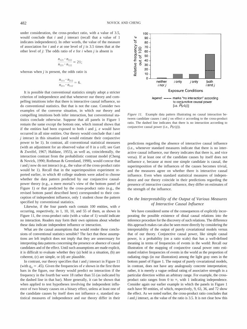
under consideration, the cross-product ratio, with a value of 3.5,would conclude that i and j interact (recall that a value of 1indicates independence). In other words, the value of the measureof association for i and e at one level of j is 3.5 times that at theother level of j: The odds ratio of e for i when j is absent is

n121 � n222

n221 � n122� 21;

whereas when j is present, the odds ratio is

n111 � n212

n211 � n112� 6.

It is possible that conventional statistics simply adopt a strictercriterion of independence and that whenever our theory and com-pelling intuitions infer that there is interactive causal influence, sodo conventional statistics. But that is not the case. Consider twoexamples of the converse situation, in which our theory andcompelling intuitions both infer interaction, but conventional sta-tistics conclude otherwise. Suppose that all panels in Figure 1remain the same except the bottom one, which instead shows thatif the entities had been exposed to both i and j, e would haveoccurred in all nine entities. Our theory would conclude that i andj interact in this situation (and would estimate their conjunctivepower to be 1). In contrast, all conventional statistical measures(with an adjustment for an observed value of 0 in a cell; see Gart& Zweifel, 1967; Haldane, 1955), as well as, coincidentally, theinteraction contrast from the probabilistic contrast model (Cheng& Novick, 1990; Rothman & Greenland, 1998), would concur thati and j now do not interact (e.g., the value of the cross-product ratiowould be 1). Recall that in the superimposition experiment re-ported earlier, in which 40 college students were asked to choosewhether the data pattern predicted by our conjunctive causal-power theory (e.g., a mere mortal’s view of the bottom panel ofFigure 1) or that predicted by the cross-product ratio (e.g., therevised bottom panel described here) corresponded to their con-ception of independent influence, only 1 student chose the patternspecified by conventional statistics.

Likewise, if the four panels each contain 100 entities, with eoccurring, respectively, in 1, 10, 10, and 55 of them, as shown inFigure 11, the cross-product ratio (with a value of 1) would indicateno interaction. Readers may form their own opinions about whetherthese data indicate independent influence or interaction.

What are the causal assumptions that would render these conclu-sions of conventional statistics sensible? The fact that these assump-tions are left implicit does not imply that they are unnecessary forinterpreting data patterns concerning the presence or absence of causalcandidates and of the effect. Until such assumptions are made explicit,it is difficult to evaluate whether they (a) hold in a situation, (b) arecoherent, (c) are simple, or (d) are plausible.

In contrast, our theory specifies that i and j interact in Figure 11(with qij .45). Given the frequencies of e shown in the first threebars in the figure, our theory would predict no interaction if thefrequency in the fourth bar were 18 rather than 55 (as indicated bythe dashed line in that bar). More generally, it can be shown thatwhen applied to test hypotheses involving the independent influ-ence of two binary causes on a binary effect, unless at least one ofthe candidate causes by itself does not influence e, standard sta-tistical measures of independence and our theory differ in their

predictions regarding the absence of interactive causal influence(i.e., whenever standard measures indicate that there is no inter-active causal influence, our theory indicates that there is, and viceversa). If at least one of the candidate causes by itself does notinfluence e, because at most one simple candidate is causal, thesuperimposition of the influences of the causes becomes trivial,and the measures agree on whether there is interactive causalinfluence. Even when standard statistical measures of indepen-dence and our theory coincide in their predictions regarding thepresence of interactive causal influence, they differ on estimates ofthe strength of the influence.

On the Interpretability of the Output of Various Measuresof Interactive Causal Influence

We have considered some of the consequences of explicitly incor-porating the possible existence of distal causal relations into theinference procedure for the discovery of such relations. The differencethis approach makes can also be seen more directly by considering theinterpretability of the output of purely covariational models versusthat of our theory. Conjunctive causal power, like simple causalpower, is a probability (on a ratio scale) that has a well-definedmeaning in terms of frequencies of events in the world: Recall ourillustration of the mapping of conjunctive causal power onto esti-mated relative frequencies of events in the world as the proportion ofradiating rings (in our illustration) among the light gray ones in thebottom panel of Figure 1. The output of purely covariational models,in contrast, does not have any analogously concrete interpretation;rather, it is merely a vague ordinal rating of associative strength in aparticular direction within an arbitrary range. For example, the cross-product ratio ranges from 0 to �, with 1 indicating independence.Consider again our earlier example in which the panels in Figure 1each have 90 entities, of which, respectively, 9, 63, 36, and 72 showthe effect. As we noted earlier, the cross-product ratio concludes thati and j interact, as the value of the ratio is 3.5. It is not clear how this

Figure 11. Example data pattern illustrating no causal interaction be-tween candidate causes i and j on effect e according to the cross-productratio. The dashed line indicates that there is no interaction according toconjunctive causal power (i.e., P̃(e|ij)).


value would be mapped onto the events conveyed by that pattern ofdata. To what, exactly, does 3.5 refer?

In the case of probabilistic contrasts (Cheng & Novick, 1990,1992; Rothman & Greenland, 1998), whereas �Pij can be as largeas 2 and as small as �2, simple contrasts range only from 1 to�1.21 For example, consider a situation in which e occurs withcertainty when either i or j is present without the other but neveroccurs when neither or both of these factors is present. In this case,Equation 2 yields an interaction contrast of �2. With the comple-mentary probabilities in the four conditions, the contrast equals 2.As with the output of the cross-product ratio, it is not clear howthese contrast values map onto entities in the world. It might beargued that the range of output values from these models can beadjusted by a scale transformation (e.g., taking the log of thecross-product ratio to give a range from �� to �, with 0 indicatingno interaction). Scaling, however, does not impart additionalmeaning, and the values would remain ordinal.

Conclusions

Our results imply that a normative statistical procedure forassessing interactive causal influence would vary across cases (seeFigures 5 and 6). In particular, a different measure would applydepending on the direction of (a) each of the two simple causes and(b) the deviation of the observed frequency of e given the jointpresence of the two candidates from that expected assuming thatthe candidates exerted only their simple powers (i.e., the sign ofthe conjunctive probabilistic contrast). Such a procedure has neverpreviously been advocated and may seem complicated. The alter-native, however, is to apply a single measure, as in standardstatistics, that only sometimes yields interpretable values and thatdoes not have a concrete mapping onto events in the world.

It seems to us that, with respect to the evaluation of conjunctivecausal hypotheses, untutored reasoning is not less but more nor-mative than standard statistical measures. Our results thereforestand in contrast to the genre of psychological research that looksto mainstream formal analyses for a definition of rationality andmeasures how untutored reasoning falls short of this standard(Kahneman, Slovic, & Tversky, 1982; Meehl, 1954).

General Conclusions

We have discussed some differences in the assessment of inter-active causal influence between our causal-power approach andthe purely covariational approach. We believe that the source ofthese differences lies in the different goals of the two approaches.Under the causal-power approach, the reasoner’s goal is to infercausal power, which he or she believes to be a distal relation—onethat exists in the world, despite the fact that it is not observable andmay in various ways fail to be manifested in the covariationsobserved. In contrast, under the purely covariational approach, thereasoner’s sole goal is to compute covariation—a proximal rela-tion that exists in the reasoner’s senses. That is, he or she foregoesinferring the distal relation that produces the proximal relation,ignoring its existence altogether by having no representation of it.

Different goals yield different results. The purely covariationalapproach yields inferences that do not license predictions about theconsequences of actions. For example, despite the covariationbetween flattened snakes and the conjunction of morning school

bells and blooming daffodils, flattened snakes will not appear onthe road if one intervenes with that conjunction—say by ringingschool bells on a winter morning in a green house full of bloomingdaffodils. To override the unwarranted recommendations for ac-tion that purely covariational statistics would have implied, 20thcentury science relied on the principles of experimental design.Our analysis indicates, however, that such principles are incapableof overriding a class of such recommendations: As illustrated inthe previous section, even when such principles hold, anomalousconclusions can result from conventional statistics. In contrast, thecausal-power approach yields inferences that (a) allow the rea-soner to predict the consequences of actions, for example, thatstriking a dry match (a conjunctive cause) would light it and (b) arein accord with some compelling principles of experimental design,without the need to invoke them as overriding assumptions. Em-pirical evidence suggests that untutored reasoners adopt the causal-power approach and make causal judgments that are normative inthese senses.

21 Peter White called our attention to this problem (personal communi-cation, August 23, 1994; see also White, 1998).

References

Ahn, W., Kalish, C. W., Medin, D. L., & Gelman, S. A. (1995). The roleof covariation versus mechanism information in causal attribution. Cog-nition, 54, 299–352.

Anderson, J. R., & Sheu, C.-F. (1995). Causal inferences as perceptualjudgments. Memory & Cognition, 23, 510–524.

Bliss, C. I. (1939). The toxicity of poisons applied jointly. Annals ofApplied Biology, 26, 585–615.

Carmichael, C., & Hayes, B. K. (2001). Prior knowledge and exemplarencoding in children’s concept acquisition. Child Development, 72,1071–1090.

Cartwright, N. (1989). Nature’s capacities and their measurement. Oxford,England: Clarendon Press.

Chapman, G. B., & Robbins, S. J. (1990). Cue interaction in humancontingency judgment. Memory & Cognition, 18, 537–545.

Cheng, P. W. (1993). Separating causal laws from casual facts: Pressingthe limits of statistical relevance. In D. L. Medin (Ed.), The psychologyof learning and motivation (pp. 215–264). New York: Academic Press.

Cheng, P. W. (1997). From covariation to causation: A causal powertheory. Psychological Review, 104, 367–405.

Cheng, P. W. (2000). Causality in the mind: Estimating contextual andconjunctive causal power. In F. Keil & R. Wilson (Eds.), Cognition andExplanation (pp. 227–253). Cambridge, MA: MIT Press.

Cheng, P. W., & Holyoak, K. J. (1995). Complex adaptive systems asintuitive statisticians: Causality, contingency, and prediction. In J.-A.Meyer & H. Roitblat (Eds.), Comparative approaches to cognition (pp.271–302). Cambridge, MA: MIT Press.

Cheng, P. W., & Novick, L. R. (1990). A probabilistic contrast model ofcausal induction. Journal of Personality and Social Psychology, 58,545–567.

Cheng, P. W., & Novick, L. R. (1992). Covariation in natural causalinduction. Psychological Review, 99, 365–382.

Clifford, D., & Cheng, P. W. (2000). Tests of a causal-power theory ofconjunctive causation. Unpublished manuscript, University of Californiaat Los Angeles.

Danks, D. (2003). Equilibria of the Rescorla–Wagner model. Journal ofMathematical Psychology, 47, 109–121.

Feller, W. (1957). An introduction to probability theory and its applica-tions (2nd edition). New York: Wiley.


Fienberg, S. E. (1980). The analysis of cross-classified categorical data(2nd edition). Cambridge, MA: MIT Press.

Forsterling, F. (1989). Models of covariation and attribution: How do theyrelate to the analogy of analysis of variance? Journal of Personality andSocial Psychology, 57, 615–625.

Freedman, D., Pisani, R., & Purves, R. (1998). Statistics (3rd edition). NewYork: Norton.

Gart, J. J., & Zweifel, J. R. (1967). On the bias of various estimators of thelogit and its variance with application to quantal bioassay. Biometrika,54, 181–187.

Glymour, C. (1998). Psychological and normative theories of causal powerand the probabilities of causes. In G. F. Cooper & S. Moral (Eds.),Uncertainty in artificial intelligence (pp. 166–172). San Francisco, CA:Kaufmann.

Glymour, C. (2000). Bayes nets as psychological models. In F. Keil & R.Wilson (Eds.), Explanation and cognition (pp. 169–198). Cambridge,MA: MIT Press.

Glymour, C. (2001). The mind’s arrows: Bayes nets and graphical modelsin psychology. Cambridge, MA: MIT Press.

Glymour, C., & Cheng, P. W. (1998). Causal mechanism and probability:A normative approach. In M. Oaksford & N. Chater (Eds.), Rationalmodels of cognition (pp. 295–313). Oxford, England: Oxford UniversityPress.

Gopnik, A., Glymour, C., Sobel, D. M., Schulz, L. E., Kushnir, T., &Danks, D. (2004). A theory of causal learning in children: Causal mapsand Bayes nets. Psychological Review, 111, 3–32.

Haldane, J. B. S. (1955). The estimation and significance of the logarithmof a ratio of frequencies. Annals of Human Genetics, 20, 309–311.

Hays, W. L. (1994). Statistics (5th edition). New York: Holt, Rinehart &Winston.

Hewstone, M. R. C., & Jaspars, J. M. F. (1987). Covariation and causalattribution: A logical model of the intuitive analysis of variance. Journalof Personality and Social Psychology, 53, 663–672.

Hilton, D. J., & Slugoski, B. R. (1986). Knowledge-based causal attribu-tion: The abnormal conditions focus model. Psychological Review, 93,75–88.

Hume, D. (1987). A treatise of human nature (2nd edition). Oxford,England: Clarendon Press. (Original work published 1739)

Jenkins, H. M., & Ward, W. C. (1965). Judgment of contingency betweenresponses and outcomes. Psychological Monographs: General and Ap-plied, 79 (1, Whole No. 594), 17.

Kahneman, D., Slovic, P., & Tversky, A. (1982). Judgment under uncer-tainty. Cambridge, England: Cambridge University Press.

Kant, I. (1965). Critique of pure reason (N. K. Smith, Trans.). London:Macmillan. (Original work published 1781).

Kelley, H. H. (1967). Attribution theory in social psychology. In D. Levine(Ed.), Nebraska symposium on motivation (Vol. 15, pp. 192–238).Lincoln: University of Nebraska Press.

Kelley, H. H. (1972). Causal schemata and the attribution process. Mor-ristown, NJ: General Learning Press.

Khoury, M. J., Flanders, W. D., Greenland, S., & Adams, M. J. (1989). Onthe measurement of susceptibility in epidemiologic studies. AmericanJournal of Epidemiology, 129, 183–190.

Lien, Y., & Cheng, P. W. (2000). Distinguishing genuine from spuriouscauses: A coherence hypothesis. Cognitive Psychology, 40, 87–137.

Mackie, J. L. (1974). The cement of the universe: A study of causation.Oxford, England: Clarendon Press.

Marr, D. (1982). Vision. San Francisco: Freeman.Meehl, P. E. (1954). Clinical versus statistical prediction: A theoretical

analysis and a look at the evidence. Minneapolis: University of Minne-sota Press.

Melz, E. R., Cheng, P. W., Holyoak, K. J., & Waldmann, M. R. (1993).Cue competition in human categorization: Contingency or the Rescorla-Wagner learning rule? Comments on Shanks (1991). Journal of Exper-imental Psychology: Learning, Memory, and Cognition, 19, 1398–1410.

Nisbett, R. E., & Ross, L. (1980). Human inference: Strategies andshortcomings of social judgment. Englewood Cliffs, NJ: Prentice-Hall.

Novick, L. R., Fratianne, A., & Cheng, P. W. (1992). Knowledge-basedassumptions in causal attribution. Social Cognition, 10, 299–333.

Parducci, A. (1965). Category judgment: A range-frequency model. Psy-chological Review, 72, 407–418.

Pearl, J. (2000). Causality: Models, reasoning, and inference. Cambridge,England: Cambridge University Press.

Peterson, C. R., & Beach, L. R. (1967). Man as an intuitive statistician.Psychological Bulletin, 68, 29–46.

Rescorla, R. A., & Wagner, A. R. (1972). A theory of Pavlovian condi-tioning: Variations in the effectiveness of reinforcement and nonrein-forcement. In A. H. Black & W. F. Prokasy (Eds.), Classical condition-ing II: Current theory and research (pp. 64–99). New York: Appleton-Century-Crofts.

Rothman, K. J., & Greenland, S. (1998). Modern epidemiology. Philadel-phia, PA: Lippincott-Raven.

Schustack, M. W., & Sternberg, R. J. (1981). Evaluation of evidence incausal inference. Journal of Experimental Psychology: General, 110,101–120.

Sheps, M. C. (1958). Shall we count the living or the dead? The NewEngland Journal of Medicine, 259, 1210–1214.

Shultz, T. R. (1982). Rules of causal attribution. Monographs of the Societyfor Research in Child Development, 47 (No. 1).

Spirtes, P., Glymour, C., & Scheines, R. (2000). Causation, prediction andsearch (2nd edition). Boston: MIT Press.

Tenenbaum, J. B., & Griffiths, T. L. (2001). Structure learning in humancausal induction. In T. K. Leen, T. G. Dietterich, & V. Tresp (Eds.),Advances in neural information processing systems 13 (pp. 59–65).Cambridge, MA: MIT Press.

Tenenbaum, J. B., & Griffiths, T. L. (2003). Theory-based causal infer-ence. In S. Becker, S. Thrun, & K. Obermayer (Eds.), Advances inneural information processing systems 15 (pp. 43–50). Cambridge, MA:MIT Press.

Tversky, A., & Kahneman, D. (1983). Extensional versus intuitive reason-ing: The conjunction fallacy in probability judgment. PsychologicalReview, 90, 293–315.

Wasserman, E. A., Elek, S. M., Chatlosh, D. L., & Baker, A. G. (1993).Rating causal relations: Role of probability in judgments of response-outcome contingency. Journal of Experimental Psychology: Learning,Memory, and Cognition, 19, 174–188.

White, P. A. (1998). Causal judgement: Use of different types of contin-gency information as confirmatory and disconfirmatory. European Jour-nal of Cognitive Psychology, 10, 131–170.

Wickens, T. D. (1989). Multiway contingency tables analysis for the socialsciences. Hillsdale, NJ: Erlbaum.

Wu, M., & Cheng, P. W. (1999). Why causation need not follow fromstatistical association: Boundary conditions for the evaluation of gener-ative and preventive causal powers. Psychological Science, 10, 92–97.


Appendix

Conjunctive Power for Cases 3 and 5 Under the Assumption That the Simple Causes and theConjunctive Cause Operate in Parallel

To explain the exact difference between the sequential and parallelconceptions, we expand the power explanation of P(e|ij) under the twoconceptions for Case 3. We first fill in the derivation for the sequential(cure) conception reported earlier. Recall that according to this conception,e will occur if (a) it is produced by a and not prevented by either i or j or(b) it is produced by the conjunction of i and j. Substituting the expressionfor P̃� �(e|ij) given in its theoretical equation (see Figure 5) into thetheoretical equation for P(e|ij) for this case (Equation 20), and making useof the no-confounding condition, we obtain this expansion of P(e|ij)according to the cure conception:

P�e�ij� � P�a� � qa � �1 � pi� � �1 � pj� � qij

� P�a� � qa � qij � �1 � pi� � �1 � pj�. (A1)

Now, consider the parallel (suppressant) conception. According to thisconception, e will occur if (a) it is produced by a or by the conjunction ofi and j and (b) it is not prevented by either i or j. Thus, to generate thepower explanation of P(e|ij), one computes the probability of the union ofthe events listed in Part a and then computes the probability of theintersection of the events listed in Parts a and b, which yields (againmaking use of the no-confounding condition):

P�e�ij� � �P�a� � qa � qij � P�a� � qa � qij� � �1 � pi� � �1 � pj�

� P�a� � qa � �1 � pi� � �1 � pj� � qij � �1 � pi� � �1 � pj�

� P�a� � qa � qij � �1 � pi� � �1 � pj�. (A2)

The righthand sides (RHSs) of Equations A1 and A2 differ only in thatthere is a qij term in Equation A1 that stands alone, whereas in Equation A2the corresponding term is multiplied by (1 � pi) � (1 � pj).

This difference leads to an alternative estimate of generative conjunctivepower under the suppressant conception, namely,

qij ��P��

�1 � pi� � �1 � pj� � P̃��e�ij�. (A3)

Equation A3 differs from the corresponding theoretical equation for thecure conception (middle cell of Figure 5) in that (1 � pi) � (1 � pj) replaces1 in the denominator of the RHS. As expected according to the suppressantconception, (1 � pi) � (1 � pj) becomes the upper bound on P(e|ij), becauseeven if the generative causes succeed in producing e in all entities, only afraction of them—namely, (1 � pi) � (1 � pj)—will be prevented byneither i nor j. In contrast, the upper bound on P(e|ij) is 1 according to thecure conception.

An analogous derivation for Case 5, in which only one simple cause, i,is preventive, yields the following estimate for generative conjunctivepower under the suppressant conception:

qij ��P�

�1 � pi� � P̃��e�ij�. (A4)

Here, (1 � pi) is the upper bound on P(e|ij), rather than 1 as in the cureconception (middle equation in the bottom panel of Figure 5).

Received September 8, 2000Revision received December 18, 2002

Accepted July 27, 2003 �


assessing interactive causal influence - uclareasoninglab.psych.ucla.edu/cheng...

Documents