ashraeâ€™s guideline 14-2002 for measurement of energy and

1

ASHRAE’s GUIDELINE 14-2002 FOR MEASUREMENT OF ENERGY AND DEMAND SAVINGS: HOW TO DETERMINE WHAT WAS REALLY SAVED BY THE RETROFIT.

Jeff S. Haberl, Ph.D., P.E.

Professor & Associate Director Charles Culp, Ph.D., P.E.

Assc. Prof. & Associate Director David E. Claridge, Ph.D., P.E. Professor & Associate Director

Energy Systems Laboratory, Texas A&M University

ABSTRACT In the Fall of 2002 ASHRAE published Guideline 14-2002 to fill a need for a standard set of energy (and demand) savings calculation procedures. Guideline 14-2002 is intended to be a guideline that provides a minimum acceptable level of performance in the measurement of energy and demand savings from energy management projects applied to residential, commercial or industrial buildings. Such measurements can serve as the basis for commercial transactions between Energy Service Companies (ESCOs) and their customers, or other energy conservation providers that rely on energy savings as the basis for repayment of the costs of the retrofit. When applied properly, ASHRAE Guideline 14-2002 is expected to provide adequate assurance for the payment of services by allowing for well-specified measurement methods that provide reasonably accurate savings calculations. ASHRAE Guideline 14-2002 may also be used by governments to calculate pollution reductions from energy efficiency activities. Since Guideline 14-2002 is intended to be applied to an individual building, or a few buildings served by a utility meter, large scale utility energy conservation programs, such as those involving statistical sampling, are not addressed by Guideline 14-2002. Furthermore, metering standards and procedures for calculating savings from modifications to major industrial process loads are also not covered. This paper presents an updated1 overview of the measurement methods contained in ASHRAE Guideline 14-2002, including a discussion about how they were developed, and their intended relationship with other national protocols for measuring savings from energy conservation programs, such as the USDOE’s International Performance Measurement and Verification Protocols (IPMVP).

1 An earlier version of this paper was presented in Haberl et al. 2001, which discussed the proposed Guideline 14. This paper provides an update to the previous paper, including new references published after the Fall of 2002. At the January 2005 ASHRAE meeting TC 7.6 voted to reinstitute a committee to update Guideline 14-2002, to address many of the references in this paper.

INTRODUCTION In many buildings, the calculation of energy savings or demand savings from energy conservation measures (ECMs) can be performed by comparing measurements of energy use and/or demand from before and after implementation of the retrofit. In the simplest cases, such as the replacement of a constant-use, constant-load appliance with a more efficient constant-use, constant-load appliance, the calculation can consist of the subtraction of the post-retrofit use from the pre-retrofit use for similar periods. Unfortunately, many ECMs involve the replacement of heating, cooling or lighting equipment that are influenced by other complicating factors such as weather, and varying occupant schedules. Therefore, ASHRAE felt there was a need for a consensus guideline that can be used to calculate normalized savings that adjusts for non-ECM influences that affect energy use. WHAT IS CONTAINED IN GUIDELINE 14-2002? Guideline 14-2002 contains seven sections and three appendices. As with most guidelines, sections one through four cover the purpose, scope, utilization and definitions that pertain to the subject matter. Section five covers the requirements and common elements, including a description of the measurement approaches, common elements of the approaches, compliance requirements, and a discussion about the design and implementation of the savings measurement process. Section six covers the specific measurement approaches, including the whole-building approach, the retrofit isolation approach, and the calibrated simulation approach. Section seven covers issues involving instrumentation and data management. Due to the importance of a number of related issues, five appendices were added to the report that contains material that supplements the seventy-seven page guideline. In Annex A, supplementary information is provided about the physical measurements required

ESL-IC-05-10-50

Proceedings of the Fifth International Conference for Enhanced Building Operations, Pittsburgh, Pennsylvania, October 11-13, 2005

2

to accomplish the specific measurement approaches, including information about sensors, calibration techniques, laboratory measurement standards, cost and instrumentation error information. Annex B contains procedures and examples for determining the uncertainty of the savings analysis, including the sources of uncertainty, formula for calculating uncertainty, and discussions about the impact of uncertainty calculations on the required level of monitoring and verification (M&V). Annex C contains examples of the application of the whole-building approach and retrofit isolation approach. This is followed by Annex D that discusses the regression techniques needed to calculate savings, and finally Annex E that discuses techniques for retrofit isolation calculations. WHO CREATED GUIDELINE 14-2002 AND HOW WAS IT WRITTEN? Guideline 14-2002 was created by a committee of ASHRAE members who represented future guideline users, producers of products that would be affected by the guideline (i.e., software, hardware or services), and ASHRAE members with a general interest in the guideline. Table 1 lists the names, affiliations and status of the ASHRAE members who participated in the Guideline2. In general, the members of Guideline 14 were ASHRAE members who are widely recognized for their experience and contributions to the field of measurement and verification. As a group, the committee’s combined knowledge represented over 350 years of experience in the field of measurement and verification. Each section of Guideline 14 was assigned a primary and secondary author. The primary author was responsible for generating the first draft of the chapter. Once this was complete ownership of the chapter was then transferred to the secondary author who was responsible for coordinating the review and editing of the chapter. Any discrepancies that arose between the primary and secondary author were resolved by the full committee. All material in each chapter was reviewed and approved by the full committee. Only published, peer-reviewed analysis methods were allowed for inclusion in Guideline 14-2002. Each chapter contains the references from which the analysis methods were obtained. HOW IS GUIDELINE 14-2002 SUPPOSED TO BE USED?

2 This table was current as of the publication of Guideline 14-2002.

In general, Guideline 14-2002 addresses the determination of energy savings by comparing before and after energy use measurements, which are adjusted for non-ECM changes, that affect energy use. The basic method is shown in Figure 1 and involves the projection of energy use or demand patterns of the pre-retrofit (baseline) period into the post-retrofit period as indicated by the dashed line that begins immediately after the ECM installation. Typical adjustments to the baseline energy use or demand include weather, occupancy, and system variables. Savings represent the amount of energy use between the projected baseline and the post-retrofit consumption and are calculated using the following formula: Savings = (Baseline energy use or demand projected to Post-Retrofit conditions) minus (Post-Retrofit energy use or demand) (1) Guideline 14-2002 contains minimum compliance requirements to insure a fair level of confidence in the savings determination. These requirements are set forth in three specific approaches and include compliance paths for each approach. The approaches include: 1) Whole-building metering, 2) Retrofit isolation metering, and 3) Whole-building calibrated simulation. These approaches were provided to balance the accuracy of the chosen approach against the cost of implementation. Proper reference to Guideline 14-2002 should therefore allow for a specific approach and accuracy to be specified, for example “Savings determination shall comply with the ASHRAE Guideline 14-2002, Path 2, whole-building performance path, with a maximum allowable uncertainty of 20% at a 90% level of confidence.” The general methodology consists of the following steps, which are illustrated in the flowchart contained in Figure 2: 1. Prepare a Measurement and Verification Plan,

showing the compliance path, the metering and analysis procedures and the expected cost of implementing the measurement and verification plan throughout the post- retrofit period.

2. Measure the energy use and/or demand before the retrofits are applied (baseline). Record factors and conditions that govern energy use and demand.

3. Measure the energy use and/or demand after the retrofits are applied (post-retrofit period).

ESL-IC-05-10-50


3

Record factors and conditions that govern post-retrofit period use and demand.

4. Project the baseline and post-retrofit period energy use and demand measurements to a common set of conditions. These common conditions are normally those of the post-retrofit period, so only baseline period energy use and demand needs to be projected.

5. Calculate savings by subtracting the projected post-retrofit period use and/or demand from the projected baseline period use and/or demand.

6. Determine the uncertainty in the cumulative savings. In three of the four paths (i.e., Whole Building Performance, Retrofit Isolation, Whole Building Calibrated Simulation) this requires the determination of and reporting of the level of uncertainty in the cumulative savings computed to date. This level of uncertainty in reported savings shall not be greater than 50% of the total savings in the post-retrofit reporting period (at the 68% confidence level). In the Whole Building Prescriptive Path, the tedious uncertainty calculations are replaced by prescribed requirements (e.g., baseline data characteristics, maximum CV(RMSE), etc.).

A significant portion of the document is devoted to the detailed description of the four compliance paths, and the tasks that must be performed by the user to comply with the guideline. Special care and attention was given to every step of the process so that the guideline would be a useful document. To accomplish this, general information, and generic procedures were provided in the main body of the document, and supporting material was provided in the appendices. Furthermore, in each section, and in the appendices, additional references were provided to point the user to supplementary sources of information. WHAT ARE THE BASIC MEASUREMENT METHODS IN GUIDELINE 14-2002? The three basic measurement methods in Guideline 14-2002 include: the Whole Building Approach (prescriptive and performance), the Retrofit Isolation Approach, and the Whole Building Calibrated Simulation Approach. Whole Building Approach. The Whole Building Approach, which has also been called the Main Meter Approach, includes procedures that verify the performance of the retrofit for those projects where whole-building, pre-retrofit and post-retrofit data are available to determine the savings. In some projects

this may include consumption and demand values that are taken from sub-meters, where those meters represent a significant portion of the building or group of subsystems in the building that are being retrofitted. Examples are: university buildings, college campuses, and Armed Forces bases. The Whole Building Approach is appropriate when the total building performance is being calculated, versus the performance of a specific retrofit (i.e., retrofit isolation). Two compliance paths were created for the Whole Building Approach, which include a prescriptive path and a performance path. The Whole Building Prescriptive Path is appropriate for projects where the savings are expected to be greater than 10% of the energy or demand use, and requires that the data be continuous, and complete. The prescriptive path does not allow for any data to be excluded from either the baseline model or the post-retrofit model and has specific requirements on the statistical goodness-of-fit indicators (e.g., CV(RMSE) < 25% for energy use and < 35% for demand for 12 or more months of pre- and post-retrofit data). If one is using the Whole Building Approach but cannot comply with the requirements of the prescriptive path, then the Whole Building Performance Approach can be followed. This path allows for data gaps, and other sorts of data irregularities by requiring the user to show that the calculated uncertainty in the cumulative savings be less than 50% of the total savings reported for the post retrofit reporting period (with a confidence level of 68%). The Whole Building Path requires that the user collect periodic utility data for the facility and includes stored (i.e., dated inventory or delivery readings of coal, liquid natural gas, or oil, etc. use) and non-stored (i.e., dated readings of electricity, steam, or pipeline-supplied gas, etc. use) energy sources, and demand data (i.e., amount and date of peak electric, steam, or pipeline-supplied gas, etc., rate). The whole building method also allows for the use of whole-building interval data (i.e., 15-minute, or hourly data). Such data are necessary for savings calculations that include time of use charges, time of day or real time electricity pricing. In most instances, regression models based upon daily data provide the best statistical goodness of fit (Katipamula et al. 1995). Hourly data can also provide more accurate insight into the building’s energy use characteristics, which can be useful in determining why a building’s

ESL-IC-05-10-50


4

post-retrofit operation may be performing below expectations, or for use in fine-tuning a building’s energy systems (Claridge et al. 1994; 1996). Unfortunately, the use of interval data also requires the collection and storage of similar weather information (i.e., hourly dry bulb temperature, humidity, solar and wind data) from a reliable source such as the National Weather Service3. In most cases the models used in for the whole building method will take the form of a linear, change-point linear, or multiple variable equations: E = C + B1V1 + B2V2 + B3V3 + A1Vn + . . .(2) Where E - Energy use or demand estimated by the

equation C - Constant term in [energy units/day] or

[demand units/billing period] Bn - Coefficient of independent variable Vn in

[energy units/driving variable units/day] or [demand units/driving variable units/day]

A1 - Coefficient of the independent variable for any adjustment(s)

Vn - Independent driving variable. Models that have been recognized as the most appropriate for modeling monthly and daily commercial building energy use include: constant or mean models, day-adjusted models, two-parameter linear models, three, four or five-parameter change-point linear models, variable-based degree day models, and multivariate linear and change-point linear models as indicated in Table 2, and as shown in Figure 3. These models represent the most widely used models for calculating baseline energy use in commercial and institutional buildings (Claridge et al. 1991; Fels 1986; Fels et al. 1995, 1996; Kissock et al. 1994; Reddy et al. 1997a, 1997b; Reynolds and Fels 1988; Ruch and Claridge 1991, 1993; Ruch et al. 1993). Software for calculating the models included in Table 2 has been developed for public distribution by ASHRAE under Research Project 1050 RP (Kissock et al. 2003; Haberl et al. 2003). Retrofit Isolation Approach. The retrofit isolation approach is intended for retrofits where the end use

3 NWS 2001. National Weather Service weather data, available from the National Oceanic and Atmospheric Administration for "Class A" sites in the United States. NOAA data are available from NOAA's National Climatic Data Center, 191 Patton Ave, Asheville, NC. See also www.ncdc.noaa.gov.

capacity, demand or power level can be measured during the baseline period, and the energy use of the equipment or subsystem can be measured post-installation for a short term period or continuously over time. The retrofit isolation approach can involve a continuous measurement of energy use both before and after the retrofit for the specific equipment or energy end use affected by the retrofit or measurements for a limited period of time necessary to determine retrofit savings. In most cases energy use is calculated by developing statistically representative models of the energy end use capacity (e.g., the kW or Btu/hr) and use (e.g., the kWh or Btu).

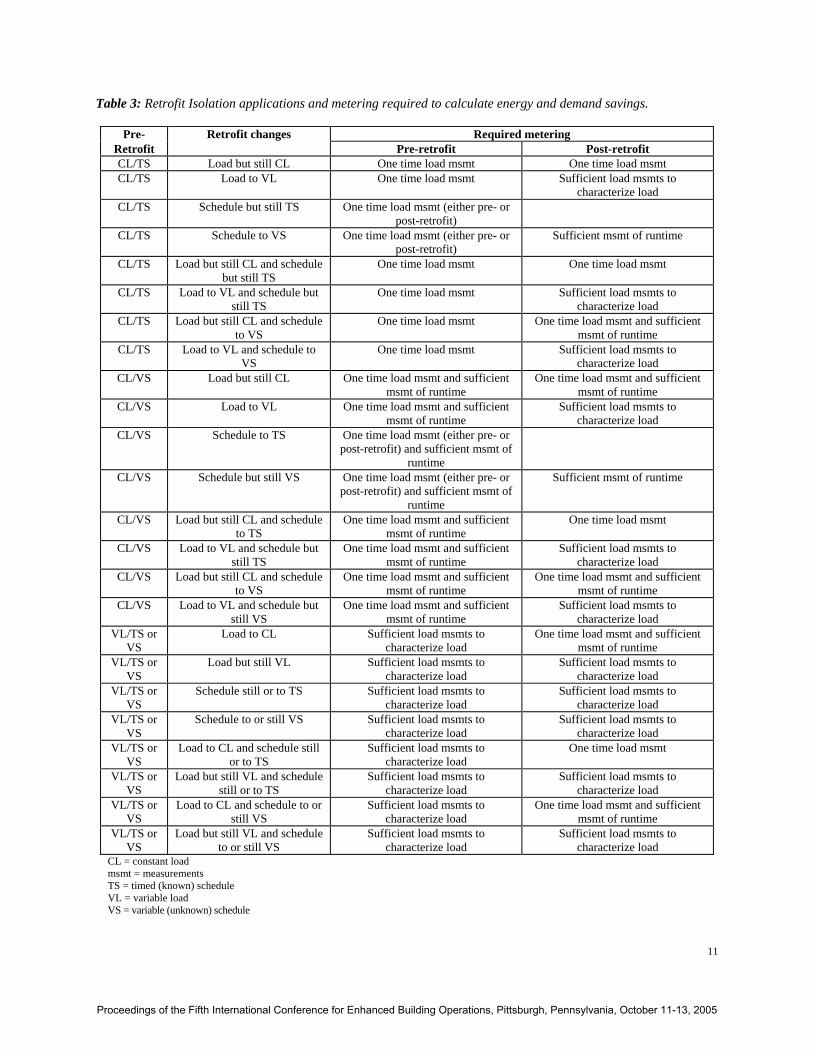
The retrofit isolation approach should be used when the whole building approach is not appropriate and the savings in question can be determined by measurements taken at a specific equipment item or subsystem. The whole building approach may not be appropriate if the savings to be determined are relatively small or if there is an unrelated change in the building served by the meter. This approach may not be appropriate for determining the individual savings from the implementation of several ECMs, when their cumulative or interactive savings cannot be determined by measurements taken at one or two specific equipment items or subsystems. Guideline 14-2002 relies heavily on previously developed standards for the laboratory measurement of temperature, pressure, airflow, liquid flow, power, thermal energy, and the testing standards for chillers, fans, pumps, motors, boilers, and furnaces. Guideline 14 also relied on the previous work that had developed in-situ measurement techniques for various energy consuming devices, including: lighting systems, pumps, blowers, chillers, thermal storage, and HVAC Systems (airside). Such work also included results from ASHRAE Research Projects 827 RP, 1004 RP, and 1093 RP. Guideline 14 has classified the retrofit isolation approach according to whether the load is fixed or variable or whether the use is constant or variable. This classification makes a distinction between constant or varying loads (i.e., different rates at which the system uses energy) versus constant or varying uses (i.e., different rates at which the system is used) primarily for purposes of measurement. This results in the following four classifications: 1. Constant Load, Constant Use. 2. Constant Load, Variable Use. 3. Variable Load, Constant Use. 4. Variable Load, Variable Use.

ESL-IC-05-10-50


5

Table 3 demonstrates how these four classifications are then used to classify the type of measurements (i.e., sufficient: one-time measurements, runtime measurements or continuous measurements) that need to be made. In the appendices that accompany Guideline 14-2002, additional advice is provided to guide the user in applying the retrofit isolation approach for: pumps (6 methods), fans (5 methods), chillers (5 methods), boilers and furnaces (12 methods), lighting (6 methods), HVAC systems (4 air-side methods), and unitary and condensing equipment (3 methods). Calibrated Simulation Approach. The whole building calibrated simulation approach involves the use of a commercially available hourly computer simulation program4 to create a model of energy use and demand of the facility. This model, which is typically a whole-building model of pre-retrofit conditions, is calibrated, or checked against actual measured energy use and demand data, measured weather data, and possibly other operating data. The calibrated model is then used to predict energy use and demand of the post-retrofit conditions. Savings are derived by comparison of modeled results under the two sets of conditions, or by comparison of modeled against actual metered results.

The whole-building calibrated simulation approach is applicable for the following conditions: 1. When accounting for multiple energy end-uses,

especially where interactions occur between measures.

2. For situations where baseline shifts may be encountered and where future energy impacts may need to be adjusted.

3. When either pre-retrofit or post-retrofit metered data are not available.

4. When measures interact with other building systems and the impact of the interaction needs to be ascertained. For example, calibrated simulation can be used to assess the cooling savings and heating increase due to a lighting retrofit.

4 Originally, this was to be limited to public domain, hourly (i.e., 8,760 hours per year), whole-building computer simulation programs such as BLAST, DOE-2 or ENERGYPLUS. However, with the advent of the completion of the ASHRAE Method of Test SMOT-140, this definition was expanded to include any commercially available computer simulation program that could be proven to be in compliance with SMOT-140. ASHRAE also has several additional research projects that are intended to strengthen future versions of SMOT-140, including Research Project 865RP.

5. When savings from individual retrofits are needed but only whole-building data are available.

Calibrated simulation should not be used under the following conditions: 1. To evaluate measures that cannot be simulated.

For example, buildings with large atriums where internal temperature stratification is significant and thermal convection is an important feature of the heating or cooling system, or buildings that contain HVAC systems that cannot readily be simulated by the software being used.

2. To evaluate retrofits that cannot be simulated. For example, radiant barriers in attics that contain exposed ductwork, or certain HVAC control changes that cannot be simulated.

3. To evaluate retrofits that are so complex that project resources will not cover the extensive computer simulation needed to adequately simulate the facility.

Calibrated simulation is normally applied in the following fashion: 1. Produce a calibrated simulation plan. This

includes selecting the appropriate simulation program, selecting the appropriate calibration approach (i.e., monthly or hourly), and determining the tolerances for calibrated simulation.

2. Collect data. Data may be collected from the building during the baseline period, the retrofit period, or both. Data collected during this step includes dimensions and properties of building surfaces, monthly and hourly whole-building utility data, nameplate data from HVAC and other building system components, operating schedules, spot-measurements of selected HVAC and other building system components, and weather data.

3. Input data into simulation software and run model. Over the course of this step, the data collected in the previous step is processed to produce a simulation-input file. Modelers are advised to take care with zoning, schedules, HVAC systems, model debugging (searching for and eliminating any malfunctioning or erroneous code), and weather data.

4. Compare simulation model output to measured data. The approach for this comparison varies depending on the resolution of the measured data. At a minimum, the energy flows projected by the simulation model are compared to monthly utility bills and spot measurements. At best, the two data sets are compared on an hourly

ESL-IC-05-10-50


6

basis. Both graphical and statistical means may be used to make this comparison.

5. Refine model until an acceptable calibration is achieved. Typically, the initial comparison does not yield a match within the desired tolerance. In such a case, the modeler studies the anomalies between the two data sets and makes logical changes to the model to better match the measured data. The user should calibrate to both pre- and post-retrofit data wherever possible and should only calibrate to post-retrofit data alone when both data sets are absolutely unavailable. While the graphical methods are useful to assist in this process, the ultimate determination of acceptable calibration will be the statistical method.

6. Produce baseline and post-retrofit models. The baseline model represents the building as it would have existed in the absence of the energy conservation measures. The retrofit model represents the building after the energy conservation measures are installed. How these models are developed from the calibrated model depends on whether a simulation model was calibrated to data collected before the conservation measures were installed, after the conservation measures were installed, or both times. Furthermore, the only differences between the baseline and post-retrofit models must be limited to the measures only. All other factors, including weather and occupancy must be uniform between the two models unless a specific difference has been observed that must be accounted for.

7. Estimate savings. Savings are determined by calculating the difference in energy flows and intensities of the baseline and post-retrofit models using the appropriate weather file.

8. Report on observations and savings. Savings estimates and observations are documented in a reviewable format. Additionally, sufficient model development and calibration documentation, including the simulation input and weather files, shall be provided to allow for accurate recreation of the baseline and post-retrofit models by informed parties.

WHAT ELSE IS CONTAINED IN GUIDELINE 14-2002? Guideline 14-2002 also contains a wealth of additional information that was included to provide as much guidance to the user as possible, including information concerning instrumentation and data management, measurement types, procedures for

determining uncertainty, laboratory testing standards, information about regression procedures, information about retrofit isolation procedures, and a generic procedure for applying the retrofit isolation. Such information is provided in several sections of the guideline and in informative indices. Instrumentation and data management. Guideline 14-2002 contains extensive recommendations about the choice of instruments, including: information regarding temperature, humidity, liquid flow meters, air flow meters, steam flow, thermal flow, pressure, and electricity measurements. Guideline 14-2002 contains advice about the installation of instruments, instrumentation calibration, recalibration and maintenance methods. Information is also provided about the selection of data recording devices, data recording intervals, retrieving and archiving data, data validation methods, information about the cost of installing sensors, and data acquisition system, and information about the accuracy of different sensor types. Measurement types. Guideline 14-2002 provides information about the duration of measurements, including: spot measurements, short-term measurements, and long-term measurements. Determination of uncertainty. One of the most useful sections of Guideline 14-2002 will most likely be the discussion about the determination of uncertainty. Extensive information is provided regarding the calculation of uncertainty, including procedures for estimating sampling error, measurement error, model prediction uncertainty, and procedures for calculating the end-to-end uncertainty. Laboratory equipment testing standards. Another very useful section in Guideline 14-2002 is the comprehensive listing of ASTM, ASME, ANSI and ASHRAE testing standards that covers a broad range of equipment, including: chillers, fans, pumps, electrical motors, boilers and furnaces, thermal storage systems, and air-side HVAC systems. Regression techniques. Guideline 14-2002 also provides extensive advice regarding the most widely used regression procedures, including: one parameter or mean models (1P), two parameter linear models (2P), three parameter change-point models for cooling or heating (3PC or 3PH), four parameter change-point models for cooling or heating (4PC or 4PH), and five parameter change-point models for systems that heat and cool (5P). Information is also provided about eliminating net bias, procedure for

ESL-IC-05-10-50


7

considering multiple variables, models based on indoor and outdoor temperature, and variable-based degree day models. Retrofit isolation approaches. Guideline 14-2002 provides 41 detailed procedures for applying the retrofit isolation approach to different types of HVAC equipment including: pumps (6 methods), fans (5 methods), chillers (5 methods), boilers and furnaces (12 methods), lighting (6 methods), HVAC systems (4 air-side methods), and unitary and condensing equipment (3 methods). SUMMARY ASHRAE has developed Guideline 14-2002 to fill a need for a standard set of energy (and demand) savings calculation procedures. Guideline 14-2002 is intended to be a guideline that provides a minimum acceptable level of performance in the measurement of energy and demand savings from energy management projects applied to residential, commercial or industrial buildings. Guideline 14-2002 was created by a committee of ASHRAE members who are widely recognized for their experience and contributions to the field of measurement and verification. Guideline 14-2002 contains minimum compliance requirements to insure a fair level of confidence in the savings determination. These requirements are set forth in three specific approaches and include compliance paths for each approach. The approaches include: 1) Whole-building metering, 2) Retrofit isolation metering, and 3) Whole-building calibrated simulation. Guideline 14-2002 also contains a wealth of additional information that was included to provide as much guidance to the user as possible, including information concerning instrumentation and data management, measurement types, procedures for determining uncertainty, laboratory testing standards, information about regression procedures, information about retrofit isolation procedures, and a generic procedure for applying the retrofit isolation. REFERENCES ASHRAE 2002. ASHRAE Guideline 14-2002 for Measurement of Energy and Demand Savings, American Society of Heating, Refrigeration and Air Conditioning Engineers, Atlanta, GA. Claridge, D., Haberl, J., O'Neal, D., Heffington, W., Turner, D., Tombari, C., Roberts, M. and Jaeger, S.

1991. “Improving Energy Conservation Retrofits with Measured Results,” ASHRAE Journal, Vol.33, No.10, pp.14-22 (October). Claridge, D., Haberl, J., Liu, M., Athar, A. 1996. “Implementation of Continuous Commissioning in the Texas LoanSTAR Program: Can you Achieve 150% of Estimated Retrofit Savings: Revisited,” Proceedings of the 1996 ACEEE Summer Study (August). Fels, M. (ed.) 1986. Energy and Buildings, Vol. 9, Nos. 1&2, Elsevier, Sequoia S.A., Lausanne, Switzerland (February/May). Fels, M., Reynolds, C., Stram, D. 1996. “PRISMonPC: The Princeton Scorekeeping Method. Documentation for Heating-Only or Cooling-Only Estimation Program: Version 4.0,” Center for Energy and Environmental Studies Report Number 213A, Princeton University (October). Fels, M.F., Kissock, K. Marean, M., Reynolds C. 1995. PRISM (Advanced Version 1.0) Users’ Guide, Center for Energy and Environmental Studies, Princeton University, Princeton, NJ, January. Haberl, J., Reeves, G., Gillespie, K., Claridge, D., Cowan, J., Culp, C., Frazell, W., Heinemeier, K., Kromer, S., Kummer, J., Mazzucchi, R., Reddy, A., Schiller, S., Sud, I., Wolpert, J., Wutka, T. 2001. “ASHRAE’s Proposed Guideline 14P for Measurement of Energy and Demand Savings: How to Determine what was Really Saved by the Retrofit,” Proceedings of the 1st International Conference for Enhanced Building Operation, Austin, TX, pp. 25-36 (July). Haberl, J., Claridge, D., Kissock, K. 2003. “Inverse Model Toolkit (1050RP): Application and Testing,” ASHRAE Transactions-Research, Vol. 109, Part 2, pp. 435-448. Katipamula, S., Reddy, T.A., Claridge, D. 1995. “Effect of Time Resolution on Statistical Modeling of Cooling Energy Use in Large Commercial Buildings,” ASHRAE Transactions 1995, Vol. 101, Part 2. Kissock, J.K., Claridge, D.E., Haberl, J.S., Reddy, T.A. 1992. “Measuring Retrofit Savings for the Texas LoanSTAR Program: Preliminary Methodology and Results,” Proceedings of the ASME/JSES/KSES International Solar Energy Conference, pp.299-308, Hawaii (April).

ESL-IC-05-10-50


8

Kissock, K., Wu, X., Sparks, R., Claridge, D., Mahoney, J., Haberl, J. 1994. “Emodel Version 1.4d,” Energy Systems Laboratory, Texas A&M University. Reddy, T.A., Haberl, J.S., Saman, N.F., Turner, W.D., Claridge, D.E., Chalifoux, A.T. 1997a. “Baselining Methodology for Facility-Level Monthly Energy Use - Part 1: Theoretical Aspects,” ASHRAE Transactions, v. 103, Pt. 2. Kissock, K., Haberl, J., Claridge, D. 2003. “Inverse Model Toolkit (1050RP): Numerical Algorithms for Best-Fit Variable-Base Degree-Day and Change-Point Models,” ASHRAE Transactions-Research, Vol. 109, Part 2, pp. 425-434. Reddy, T.A., Haberl, J.S., Saman, N.F., Turner, W.D., Claridge, D.E., Chalifoux, A.T. 1997b “Baselining Methodology for Facility-Level Monthly Energy Use - Part 2: Application to Eight Army Installations,” ASHRAE Transactions, v. 103, Pt. 2.

Reynolds, C., Fels, M. 1988. “Reliability Criteria for Weather Adjustment of Energy Billing Data,” Proceedings of the 1988 ACEEE Summer Study on Energy Efficiency in Buildings, pp. 10.236 - 10.251, Washington, D.C. Ruch, D., Claridge, D. 1991. “A Four Parameter Change-Point model for Predicting Energy Consumption in Commercial Buildings,” Proceedings of the ASME-JSES-JSME International Solar Energy Conference, Reno, NV, March 17-22, pp. 433-440. Ruch, D.K., Claridge, D.E. 1993. “A Development and Comparison of NAC Estimates for Linear and Change-Point Energy Models for Commercial Buildings,” Energy and Buildings, Vol. 20, pp.87-95. Ruch, D.K., Kissock, J.K., Reddy, T.A., 1993. “Model Identification and Prediction Uncertainty of Linear Building Energy Use Models with Autocorrelated Residuals,” Solar Engineering 1993.

Table 1: Guideline 14 Committee Roster5. NAME AFFILIATION COMMITTEE

STATUS George Reeves George Reeves & Associates,

Lake Hopatcong, NJ Chair

Ken Gillespie PG&E, San Francisco, CA Vice Chair David Claridge Texas A&M University, College

Station, TX Non-voting Member – general interest

John Cowan Cowan Quality Buildings, Toronto, Ontario, Canada

Voting Member – producer

Charles Culp Emerson Electric, Marshalltown, IA6

Non-voting Member – producer

Wayne Frazell TXU, Ft. Worth, TX Voting Member – user Jeff Haberl Texas A&M University, College

Station, TX Voting Member – general interest

Kristin Heinemeier Honeywell, Minneapolis, MN7 Voting Member – producer Steve Kromer LBNL, Berkeley, CA8 Voting Member – user James Kummer Johnson Controls, Milwaukee, WI Voting Member – producer Richard Mazzucchi Resource Perf. Man. Silverdale,

WA9 Voting Member – general interest

Agami Reddy Drexel University, Philadelphia, PA

Voting Member – general interest

Steve Schiller Steve Schiller and Assc., Oakland, Voting Member – general interest

5 Other ASHRAE members who participated significantly in the development of Guideline 14 but were not on the Committee Roster, include: Robert Sonderegger, Silicone Energy, Inc., Berkeley, CA; and John Phelan, AEC, Boulder, CO. 6 Now at the Energy Systems Laboratory, Texas A&M University, College Station, TX. 7 Now at PECI in San Diego, CA. 8 Now at Enron, Houston, TX. 9 Now at Seattle City Light, Seattle, WA.

ESL-IC-05-10-50


9

CA Ish Sud Sud Associates, Durham, NC Voting Member – general interest Jack Wolpert E-cube, Boulder, CO Voting Member – user Thomas Wutka HEC Inc., North Granby CT Voting Member – producer

ESL-IC-05-10-50


10

Table 2: Sample Models for Whole Building Approach

Name Independent Variable(s) Form Examples No Adjustment /Constant Model

None E = Eb Non weather sensitive demand

Day Adjusted Model None E = Eb x dayb dayc

Non weather sensitive use (fuel in summer, electricity in summer)

Two Parameter Model Temperature E = C +B1(T) Three Parameter Models Degree days/Temperature E = C + B1(DDBT)

E = C + B1(B2 – T)+

E = C + B1(T – B2)+

Seasonal weather sensitive use (fuel in winter, electricity in summer for cooling) Seasonal weather sensitive demand

Four Parameter, Change Point Model

Temperature E = C + B1(B3 - T)+ - B2(T - B3)+

E = C - B1(B3 - T)+ + B2(T - B3)+

Five Parameter Models Degree days/Temperature E = C - B1(DDTH) + B2(DDTC) E = C + B1(B3 - T)+ + B2(T - B4)+

Heating and cooling supplied by same meter.

Multi-Variate Models Degree days/Temperature, other independent variables

Combination form Energy use dependent non-temperature based variables (occupancy, production, etc.).

Sep-92 Mar-93 Sep-93 Mar-94 Sep-94 Mar-95 Sep-95 Mar-96 Sep-96

Ene

rgy

Use

Post Retrofit Use

Baseline Use

Baseline Period Post Retrofit Period

Adjusted Baseline Use

ECM Installation

Savings

Figure 1: Guideline 14’s basic method for determining savings.

ESL-IC-05-10-50


11

Table 3: Retrofit Isolation applications and metering required to calculate energy and demand savings.

Pre- Retrofit changes Required metering Retrofit Pre-retrofit Post-retrofit CL/TS Load but still CL One time load msmt One time load msmt CL/TS Load to VL One time load msmt Sufficient load msmts to

characterize load CL/TS Schedule but still TS One time load msmt (either pre- or

post-retrofit)

CL/TS Schedule to VS One time load msmt (either pre- or post-retrofit)

Sufficient msmt of runtime

CL/TS Load but still CL and schedule but still TS

One time load msmt One time load msmt

CL/TS Load to VL and schedule but still TS

One time load msmt Sufficient load msmts to characterize load

CL/TS Load but still CL and schedule to VS

One time load msmt One time load msmt and sufficient msmt of runtime

CL/TS Load to VL and schedule to VS

One time load msmt Sufficient load msmts to characterize load

CL/VS Load but still CL One time load msmt and sufficient msmt of runtime

One time load msmt and sufficient msmt of runtime

CL/VS Load to VL One time load msmt and sufficient msmt of runtime

Sufficient load msmts to characterize load

CL/VS Schedule to TS One time load msmt (either pre- or post-retrofit) and sufficient msmt of

runtime

CL/VS Schedule but still VS One time load msmt (either pre- or post-retrofit) and sufficient msmt of

runtime

Sufficient msmt of runtime

CL/VS Load but still CL and schedule to TS


One time load msmt

CL/VS Load to VL and schedule but still TS



CL/VS Load but still CL and schedule to VS



CL/VS Load to VL and schedule but still VS



VL/TS or VS

Load to CL Sufficient load msmts to characterize load


VL/TS or VS

Load but still VL Sufficient load msmts to characterize load


VL/TS or VS

Schedule still or to TS Sufficient load msmts to characterize load


VL/TS or VS

Schedule to or still VS Sufficient load msmts to characterize load


VL/TS or VS

Load to CL and schedule still or to TS


One time load msmt

VL/TS or VS

Load but still VL and schedule still or to TS



VL/TS or VS

Load to CL and schedule to or still VS



VL/TS or VS

Load but still VL and schedule to or still VS



CL = constant load msmt = measurements TS = timed (known) schedule VL = variable load VS = variable (unknown) schedule

ESL-IC-05-10-50


12

General Approach ForMeasurement Of Energy And

Demand Savings

Prepare M & V Plan showing CompliancePath.

Measure Baseline energy use andrecord governing conditions.

Measure Post-Retrofit energy use andrecord governing conditions.

Project Baseline andPost-Retrofit energy use to a

common set of conditions (usuallyPost-Retrofit conditions).

Projected Baseline useminus Projected

Post-Retrofit use = Savings.

Report Savings, (and Uncertainty iffollowing a Performance Compliance

Path).

Figure 2: Guideline 14’s general approach for measurement of energy and demand savings.

ESL-IC-05-10-50


13

Ambient Temperature

Ener

gy U

sage

Ambient Temperature

Ener

gy U

sage

Ambient Temperature

Ener

gy U

sage

Ambient Temperature

Ener

gy U

sage

Ambient Temperature

Ener

gy U

sage

Ambient Temperature

Ener

gy U

sage

Ambient Temperature

Ener

gy U

sage

Bo

Bo

B1

Bo Bo

B1B1

B2 B2

Bo Bo

B3 B3

B1

B1

B2B2

Bo

B4

B1 B2

B3

(a) (b)

(c) (d)

(e) (f)

(g)

Figure 3: Linear and Change-point Linear Models Used in Guideline 14. This figure shows several of the models used in Guideline 14, including: a) mean or constant model; b) two parameter linear models; three parameter change-point linear models for c) heating and d) cooling; four parameter change-point linear models for e) heating and f) cooling; and g) a five parameter change-point linear model.

ESL-IC-05-10-50


ashraeâ€™s guideline 14-2002 for measurement of energy and

Documents