measurement and verification (m&v) guideline for federal
TRANSCRIPT
M&VM&VM&VM&VM&VM&VM&VM&VM&V
F E D E R A L E N E R G Y M A N A G E M E N T P R O G R A M
M&V Guidelines:Measurement and Verification for Federal Energy Projects
Version 2.2
U . S . D E PA R T M E N T O F E N E R G YO F F I C E O F E N E R G Y E F F I C I E N C Y A N DR E N E WA B L E E N E R G Y
DOE/GO-102000-0960September 2000

ATTENTION
Thank you for your interest in Federal Energy Management and the Federal Energy Management Program’s (FEMP) M&V Guidelines: Measurement and Verification for Federal Energy Projects, Ver-sion 2.2. This document is designed for use in contracts between federal agencies and energy ser-vice companies, utilities, and others.
The FEMP M&V Guidelines contain specific procedures for applying concepts originating in the International Performance Measurement and Verification Protocol (IPMVP). The IPMVP, formerly the North American Energy Measurement and Verification Protocol, was developed through a col-laborative effort involving industry, government, financial, and other organizations. The IPMVP provides the framework for M&V procedures and addresses issues related to the use of M&V in third-party financed and utility projects.
For more information, see section 1.4 of the M&V Guidelines. Copies of the IPMVP can be found on the World Wide Web at the IPMVP site: http://www.ipmvp.org/. For information on updates to FEMP’s M&V Guidelines, visit the FEMP Web site at http://www.eren.doe.gov/femp/financing/meas-guide.html.
Tell us what you think!We’re interested in your response to the M&V Guidelines. We will use the information you provide below to help us improve future ver-sions of the Guidelines and create other ways to help you verify energy savings.
Please return to Dale Sartor, Lawrence Berkeley National Laboratory, MS90-3111, Berkeley, CA, 94720; phone: 510-486-5988; e-mail: [email protected]
1. Where did you hear of the M&V Guidelines? workshop FEMP help desk Federal Register Web siteother (please specify):
2. How did you obtain your copy? workshop FEMP help desk request for proposal referenceWeb site other (please specify):
3. How did you (or how will you) use the Guidelines?
4. What information did you look for but did not find in the Guidelines?
5. What would you suggest changing or adding in future editions?
6. What is the name of your organization?
If you’d like to be contacted for further comments, please write your name and phone number or e-mail address in the space below:
M&V Guidelines:Measurement and Verification for Federal Energy Projects
Version 2.2
Prepared For:U.S. Department of Energy
Federal Energy Management ProgramEE-90, 1000 Independence Ave., SW
Washington, DC 20585 Tel. 202-586-5772
Internet: http://www.eren.doe.gov/femp
Prepared By:Schiller Associates
1333 Broadway, Suite 1015Oakland, CA 94612Tel. 510-444-6500
Under Subcontract To:National Renewable Energy LaboratoryLawrence Berkeley National Laboratory

NOTICE
This report was prepared as an account of work sponsored by an agency of the United Statesgovernment. Neither the United States government nor any agency thereof, nor any of their employees,makes any warranty, express or implied, or assumes any legal liability or responsibility for the accuracy,completeness, or usefulness of any information, apparatus, product, or process disclosed, or representsthat its use would not infringe privately owned rights. Reference herein to any specific commercialproduct, process, or service by trade name, trademark, manufacturer, or otherwise does not necessarilyconstitute or imply its endorsement, recommendation, or favoring by the United States government or anyagency thereof. The views and opinions of authors expressed herein do not necessarily state or reflectthose of the United States government or any agency thereof.
Available electronically at http://www.doe.gov/bridge
Available for a processing fee to U.S. Department of Energyand its contractors, in paper, from:
U.S. Department of EnergyOffice of Scientific and Technical InformationP.O. Box 62Oak Ridge, TN 37831-0062phone: 865.576.8401fax: 865.576.5728email: [email protected]
Available for sale to the public, in paper, from:U.S. Department of CommerceNational Technical Information Service5285 Port Royal RoadSpringfield, VA 22161phone: 800.553.6847fax: 703.605.6900email: [email protected] ordering: http://www.ntis.gov/ordering.htm
Printed on paper containing at least 50% wastepaper, including 20% postconsumer waste

Acknowledgments
This document was prepared by Steven R. Schiller, David A. Jump, Ellen M. Franconi, Mark Stetz, and Andrea Geanacopoulos of Schiller Associates, Oakland, California, and
Boulder, Colorado. (www.schiller.com)
The document follows the U.S. Department of Energy's (DOE's) International Perfor-mance Measurement and Verification Protocols (IPMVP).
Contributors to this document include: Dale Sartor of Lawrence Berkeley National Labo-ratory, Doug Dahle of the National Renewable Energy Laboratory, and Erica Atkin of the
Oak Ridge National Laboratory.
Table of Contents
Overview of Guidelines 2.2 ...................................................................................................................... 1
Section I: ESPC Program Description and M&V Overview 3
Chapter 1: Purpose and Program Description....................................................................................... 4Chapter 2: Measurement and Verification: An Overview...................................................................... 9
Section II: Incorporating M&V into ESPCs 35
Chapter 3: Overview of M&V Procedural Steps and Submittals ........................................................... 36Chapter 4: M&V Plan Preparation and Review ...................................................................................... 41Chapter 5: M&V Quick-Start Guidelines ................................................................................................ 56
Section III: Selected M&V Methods—Option A 65
Chapter 6: Introduction to Option A ..................................................................................................... 66Chapter 7: Lighting Efficiency: No Metering and Metering of Fixture Wattages Only....................... 69Chapter 8: Lighting Controls: No Metering and Metering of Fixture Wattages Only ........................ 75Chapter 9: Constant-Speed Motor Efficiency: Metering of Motor kW ................................................. 82Chapter 10: Variable-Speed Drive Motor Efficiency: Metering of Motor kW ...................................... 88Chapter 11: Chiller Replacement: No Metering and Verification of Chiller kW/ton Methods......... 94
Section IV: Selected M&V Methods—Option B 101
Chapter 12: Introduction to Option B.................................................................................................... 102Chapter 13: Lighting Efficiency: Monitoring of Operating Hours ....................................................... 104Chapter 14: Lighting Efficiency: Metering of Lighting Circuits ........................................................... 111Chapter 15: Lighting Controls: Monitoring of Operating Hours......................................................... 118Chapter 16: Lighting Controls: Metering of Lighting Circuits ............................................................. 126Chapter 17: Constant-Load Motor Efficiency: Metering of Operating Hours ..................................... 133Chapter 18: Variable-Speed Drive Retrofit: Continuous Post-Installation Metering ........................... 142Chapter19: Chiller Replacement: Metering of kW and of kW and Cooling Load............................... 150Chapter 20: Generic Variable Load: Continuous Post-Installation Metering ...................................... 157
Section V: Whole Building M&V—Option C 163
Chapter 21: Introduction to Option C ................................................................................................... 164Chapter 22: Utility Billing Analysis Using Regression Models .............................................................. 168Chapter 23: Utility Bill Comparison with a Discussion of Energy Accounting .................................... 175
Section VI: Whole-Building Computer Simulation—Option D 183
Chapter 24: Introduction to Option D ................................................................................................... 184Chapter 25: Calibrated Computer Simulation Analysis......................................................................... 190
Section VII: M&V for Water Projects 203
Chapter 26: Introduction to Water Conservation Measurement and Verification.............................. 204Chapter 27: Stipulated Flows and Operating Schedules for Plumbing Devices .................................. 223Chapter 28: Metered Flows and Stipulated or Metered Durations for Plumbing Devices .................. 228Chapter 29: All Water Uses Compatible with Sub-Metering or Monitoring ........................................ 234Chapter 30: All Water Uses Compatible with Whole-Facility Metering ................................................ 238Chapter 31: Calibrated Simulation Analysis of Water-Consuming Systems ......................................... 243
Section VIII: M&V Plan Overviews for Other Project Categories 249
Chapter 32: New Construction Projects.................................................................................................. 250Chapter 33: Operations and Maintenance Measures ............................................................................ 265Chapter 34: Cogeneration Projects......................................................................................................... 274Chapter 35: Renewable Energy Projects ................................................................................................. 281
Appendices
Appendix A: Definition of Terms ........................................................................................................... 287Appendix B: Sample Metering Forms..................................................................................................... 290Appendix C: Sample Lighting and Motor Survey Forms....................................................................... 293Appendix D: Sampling Guidelines ......................................................................................................... 308
Overview of Guidelines 2.2
The Energy Policy Act of 1992 and Executive Order 13123 direct federal buildingmanagers to reduce energy consumption per square foot by 20 percent by the year 2000, 30 percent by the year 2005, and 35 percent by the year 2010, relative to a 1985 baseline. The Federal Energy Management Program (FEMP) is helping achieve these goals by encouraging the utilization of private sector technical expertise and invest-ment resources through the use of energy savings performance contracts (ESPC).
In an ESPC, a third party purchases and installs new equipment at a federal agency's facility. In exchange, the third party receives a share of the federal agency's savings in energy costs. Since compensation is based on project energy savings, the law underlying the authority for federal facilities to enter into ESPCs requires that energy savings be verified, reducing the agency's risk. The challenge is to balance costs and savingscertainty with the value of the measures that are installed at the facility. (The intent of Congress is to have the resultant energy cost savings from a project meet or exceed the cost of its implementation.)
The purpose of this document is to provide guidelines and methods for measuring and verifying the savings associated with federal agency performance contracts. It contains procedures and guidelines for quantifying the savings resulting from energy efficiency equipment, water conservation, improved operation and maintenance, renewable energy, and cogeneration projects implemented under federal agency-financed ESPCs.
Section I of the Guidelines describes ESPC programs and provides a general overview of measurement and verification (M&V). Section II outlines M&V procedural steps and describes M&V issues in detail. It also provides quick reference tables and checklists for preparing and reviewing M&V plans. Sections III through VIII describe standardized M&V methods that should be used with federal performance contracts for energy projects, water projects, and other project categories.
M&V Guidelines: Measurement and Verification for Federal Energy Projects, Version 2.2 1


M&V Guidelines:
Section I:ESPC Program Description and
M&V Overview
This section contains two chapters. It introduces federal energy savingperformance contracts (ESPC) and provides an overview of generalmeasurement and verification (M&V) procedures. Chapter 1 discusses thepurpose and scope of the document, program descriptions, and programresources. Chapter 2 describes general M&V concepts and issues associatedwith federal ESPCs.
• Chapter 1: Purpose and Program Description
• Chapter 2: Measurment and Verification: an Overview
Measurement and Verification for Federal Energy Projects, Version 2.2 3
1
Purpose and Program Description
1.1 ESPC Program Background
The Federal Energy Management Program (FEMP) was established within the U.S. Department of Energy to assist federal agencies in reducing facility costs. Many federal facilities can benefit from improved energy performance, reduced energy expendi-tures, and greater occupancy comfort. In addition, Executive Order 13123, signed by President Clinton on June 3, 1999, raises the energy use reduction goals for federal facilities. It establishes a goal to reduce energy consumption per square foot by 20percent by the year 2000, 30 percent in 2005, and 35 percent in 2010, relative to a 1985 baseline.
By making capital investments in energy conservation measures (ECMs), federal facility managers can often reduce operating expenditures substantially. Frequently, however, capital funds are not available for such projects. A third party may see this lack of capi-tal as an opportunity to purchase and install new equipment at a facility in exchange for a share of the federal agency's energy cost savings. If the third party guarantees aspecific level of savings, the arrangement is known as an energy savings performance contract, or ESPC. For contracts with federal agencies, both energy service companies (ESCOs) and electric utilities may act as third parties.
An ESPC can apply to contracts involving renewable energy systems, water conserva-tion, operations and maintenance (O&M) improvements, and other measures, as well as to contracts involving energy conservation measures and energy-efficient systems. Thus, here, “energy” is a generic term that includes fuel and electricity as well as water.
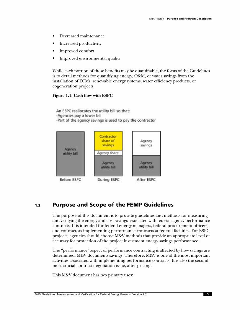
In an ESPC, a third party makes an investment in a facility that reduces its operating (primarily energy) costs. The third party then receives periodic payments from the agency that come from a share of the reduced cost savings. Figure 1.1 illustrates how the ESPCs work. After the contract period ends, the agency retains all of the savings.
A federal facility may enter into a performance contract to reduce overall energy use and/or to obtain new equipment. The contract can apply to both new construction and retrofits. The energy savings realized provide an income stream that will finance the project. In many cases, older, outdated equipment will be replaced with new equipment and control systems. As a direct result of the equipment change-out, the federal facility may also realize savings from:
M&V Guidelines: Measurement and Verification Guideline Federal Energy Projects, Version 2.24
CHAPTER 1
Purpose and Program Description
• Decreased maintenance
• Increased productivity
• Improved comfort
• Improved environmental quality
While each portion of these benefits may be quantifiable, the focus of the Guidelines is to detail methods for quantifying energy, O&M, or water savings from theinstallation of ECMs, renewable energy systems, water efficiency products, orcogeneration projects.
Figure 1.1: Cash flow with ESPC
1.2 Purpose and Scope of the FEMP Guidelines
The purpose of this document is to provide guidelines and methods for measuring and verifying the energy and cost savings associated with federal agency performance contracts. It is intended for federal energy managers, federal procurement officers, and contractors implementing performance contracts at federal facilities. For ESPC projects, agencies should choose M&V methods that provide an appropriate level of accuracy for protection of the project investment energy savings performance.
The “performance” aspect of performance contracting is affected by how savings are determined. M&V documents savings. Therefore, M&V is one of the most important activities associated with implementing performance contracts. It is also the second most crucial contract negotiation issue, after pricing.
This M&V document has two primary uses:
M&V Guidelines: Measurement and Verification for Federal Energy Projects, Version 2.2 5

SECTION I
ESPC Program Description and M&V Overview
• It serves as a reference document for specifying M&V methods and procedures in delivery orders, requests for proposals (RFPs), and performance contracts.
• It is a resource for those developing project-specific M&V plans for federalperformance contracting projects.
By using this document, federal agencies will have confidence that their projects are verified (with respect to what was installed and the savings achieved). They will have followed procedures that can be applied with consistency to similar projects through-out all geographic regions and that are impartial, reliable, and repeatable.
This is Version 2.2 (2000) of the Guidelines; Version 2.0 was published in 1996. This version contains the following updates to the 1996 version:
• A discussion of ESPC responsibility issues and how they affect risk allocation.
• Quick M&V guidelines including procedural outlines, content checklists, and option summary tables.
• Measure-specific guidelines for assessing the most appropriate M&V option for common measures.
• New M&V strategies and methods for cogeneration, new construction,operations and maintenance, renewable energy systems, and waterconservation projects.
• Editorial updates of the chapters for improved content consistency andreadability.
1.3 How to Use the Guidelines
The M&V Guidelines are a general reference and guide to specifying measurement and verification methods for federal ESPCs. The Guidelines are divided into 8sections consisting of 35 chapters, plus 4 appendices; at the front of each section isa brief summary of the section chapters' contents:
• Section I, Chapters 1 and 2, provides an introduction to ESPC concepts and an overview of M&V. Chapter 2, Tables 2.3–2.5 provide a summary and index of the measure-specific M&V methods included in this document.
• Section II, Chapters 3 through 5, gives procedures for incorporating M&V in an ESPC. Chapter 3 is an overview of the process. Chapter 4 describes detailsassociated with M&V plan preparation. Chapter 5 presents “quick-start”Guidelines references including summary tables and checklists.
• Sections III, IV, V, and VI contain descriptions of measure-specific M&V methods for energy retrofits; these four sections discuss M&V methods that are based on M&V Options A, B, C, and D, respectively.
• Section VII, Chapters 26 through 31, contains descriptions of measure-specific M&V methods for water conservation measures.
M&V Guidelines: Measurement and Verification for Federal Energy Projects, Version 2.26
CHAPTER 1
Purpose and Program Description
• Section VIII, Chapters 32 through 35, presents M&V method descriptions for other types of measures including new construction, operation and maintenance, cogeneration, and renewable energy.
It is recommended that readers new to M&V read through Sections I, II, andAppendix A (definition of terms) in their entirety. Once the basics are understood, the reader can choose which parts of the remaining sections address the specific needs of the ESPC project in which he or she is involved. For example, if the project involves a lighting efficiency measure, the reader should study the M&V methods summarized in Table 5.2 (Lighting Efficiency Retrofits—M&V Methods andResponsibilities), evaluate the level of risk allowable for the measure, make apreliminary selection of the appropriate M&V method, and read the detailed description of the method (i.e., method LE-B-01, presented in Chapter 13).
For readers more familiar with M&V plan development, the summary documents presented in Chapter 5 provide a quick reference to the procedures and compo-nents associated with M&V plan preparation and review. Chapter 2 describescontract responsibility issues, which are summarized in Table 2.1 and described in section 2.2.1. Responsibility issues that impact cost-savings risk allocation is an impor-tant new topic that needs to be understood before developing an ESPC. Chapters 3 and 4 provide details that are worth reviewing concerning M&V plan development.
1.4 ESPC Program M&V Resources
Measuring and verifying savings from ESPC projects requires special projectplanning and engineering activities. M&V is an evolving science, although several common practices exist. These practices are documented in several resources described below and include the International Performance Measurement andVerification Protocol (IPMVP) and the American Society of Heating, Refrigerating, and Air-Conditioning Engineers (ASHRAE) Guide 14P. These resources may beclassified as general protocols (IPMVP), technical guidelines (ASHRAE 14P), or application-specific guidelines (FEMP Guidelines 2.2).
1.4.1 IPMVPThe 1998 IPMVP is a voluntary consensus document written by and for technical, procurement, and financial personnel in government, commerce, and industry. The IPMVP provides an overview of current M&V techniques and sets a framework for verifying third-party-financed energy projects for public (including federal) andprivate sector projects. The IPMVP is intended to be used as the basis for preparing program M&V guidelines, such as this document. The FEMP M&V Guidelinesrepresent a specific application of the IPMVP to federal projects. The FEMPGuidelines outline procedures for specifying M&V in the preparation of requests for proposals, for evaluating proposals, and for establishing the basis of payment for energy savings during the contract. They are intended to be fully compatible and consistent with the IPMVP. For more information on the IPMVP, visit the web site at http://www.ipmvp.org.
M&V Guidelines: Measurement and Verification for Federal Energy Projects, Version 2.2 7
SECTION I
ESPC Program Description and M&V Overview
1.4.2 ASHRAE Guideline 14ASHRAE Guideline 14: Measurement of Energy & Demand Savings, First Public Review Draft, April 2000, is a proposed guideline for calculating energy savingsassociated with performance contracts. It introduces generic M&V approaches and describes detailed analysis procedures associated with completing M&V. In addition, it presents instrumentation and data management guidelines and describes methods for accounting for uncertainty associated with models and measurements. (For more information, please visit the Web site at http://www.ahsrae.org.)
1.4.3 FEMP ResourcesThe FEMP M&V Guidelines provide guidance on selecting the appropriate M&V effort for ESPC projects. It does not, however, contain detailed cost/benefitguidelines on selecting an M&V approach, establishing an appropriate level ofaccuracy, and creating a budget for the many different energy conservationmeasures (ECMs) and particular contract situations that can occur under ESPCs.For information not covered in the Guidelines, federal agency staff can contact their DOE Regional Office for assistance (for contacts and resources, please visit the Web site at http://www/eren.doe.gov/femp/financing/femp_services_who.html).
M&V Guidelines: Measurement and Verification for Federal Energy Projects, Version 2.28
2
Measurement and Verification: An Overview
This chapter is an overview of the M&V concepts and issues associated with federal ESPCs. Also included are summaries of M&V Options A, B, C, and D. The last portion of this chapter discusses the degree of rigor required in the M&V effort.
2.1 General Approach to M&V
Facility energy (O&M or water) savings are determined by comparing the energy use before and after the installation of energy conservation measures. The “before” caseis called the baseline; the “after” case is referred to as the post-installation orperformance period. Proper determination of savings includes adjusting for changes that affect energy use but that are not caused by the conservation measures. Such adjustments may account for differences in weather and occupancy conditions between the baseline and performance periods.
In general,
Baseline and post-installation energy use can be determined using the methodsassociated with several different M&V approaches. These approaches are termed M&V Options A, B, C, and D. A range of options is available to provide suitable techniques for a variety of applications. How one chooses and tailors a specific option is based on the level of M&V rigor required to obtain the desired accuracy level in the savings determination and is dependent on the complexity of the ECM, the potential for changes in performance, and the measure savings value.
The law (Title 42, United States Code, Section 8287) underlying the authority forfederal facilities to enter into ESPCs requires guaranteed savings and, therefore, savings verification. The function of verification is to reduce agency risk. The challenge of M&V is to balance M&V costs and savings certainty with the value of the conservation measures.
Savings Baseline Energy Use( )adjusted Post-Installation Energy Use( )–=
M&V Guidelines: Measurement and Verification for Federal Energy Projects, Version 2.2 9
SECTION I
ESPC Program Description and M&V Overview
2.2 M&V Requirements
The agency must exercise diligence to ensure that the M&V incorporated into the ESPC provides the appropriate level of performance verification for the specificconservation measures. To accomplish this, the M&V must include mandatory and option-specific requirements. The mandatory requirements common to all ESPC projects are:
1. Understanding ESPC issues that impact risk allocation to the agency or ESCO. Review of responsibility issues impacting risk should be completed early in the development of the ESPC project delivery order.
2. Preparation of a project measurement and verification plan. This should becompleted early in the development of the ESPC project delivery order.
3. Documentation of the baseline conditions and verification of the potential for the conservation measures to generate savings.
4. Determination of savings in accordance with one of the four M&V options.
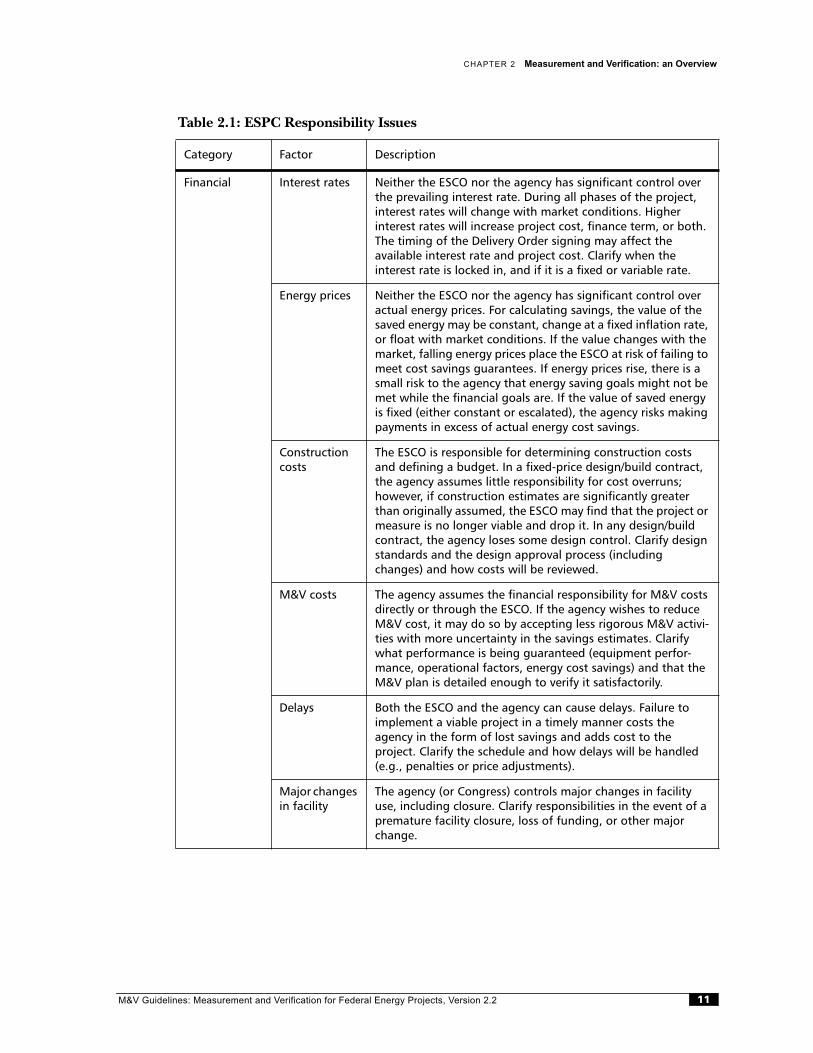
2.2.1 Contract Responsibility IssuesThere are ESPC components that inherently specify how the risks associated with achieving estimated project cost savings are allocated between the agency and the ESCO. These components are generally related to the contract financial terms and the M&V methods agreed upon to determine savings. The contract issues affecting responsibility allocation are outlined in Table 2.1. The table lists the primary factors that impact the determination of savings and illustrates how their definition indi-cates which party—the ESCO or the government agency or perhaps neither—is responsible for each factor. Factors may include equipment performance (typically the ESCO's responsibility), changes in function of facility performance (typically the agency's responsibility), changes in weather (typically neither party's responsibility), and energy prices (typically the ESCO's risk if energy prices stay within a certain range, and the agency's risk if the prices fall outside that range).
Completing a responsibility table is a useful exercise for understanding the level of rigor required in the M&V plan, as it indicates which factors are the responsibility of the ESCO and thus need to be documented during the life of the contract. Ingeneral, but not always, a contract objective may be to release the ESCO from responsibility for factors beyond its control, such as building occupancy and weather, yet hold the ESCO responsible for controllable factors (risks), such as maintenance of equipment efficiency.
To reduce risks and the level of M&V rigor required, it is important to establishreasonable savings expectations before ECM or system installation. ESCOs mayoverestimate customer savings by relying on overly optimistic energy savingscalculations. The federal agency should attempt to reach consensus with project sponsors on realistic energy savings estimates before issuing approval to proceed with installation. This approach establishes reasonable expectations up front that reduce the likelihood of a payment dispute following installation.
M&V Guidelines: Measurement and Verification for Federal Energy Projects, Version 2.210
CHAPTER 2
Measurement and Verification: an Overview
Table 2.1: ESPC Responsibility Issues
Category Factor Description
Financial Interest rates Neither the ESCO nor the agency has significant control over the prevailing interest rate. During all phases of the project, interest rates will change with market conditions. Higherinterest rates will increase project cost, finance term, or both. The timing of the Delivery Order signing may affect theavailable interest rate and project cost. Clarify when theinterest rate is locked in, and if it is a fixed or variable rate.
Energy prices Neither the ESCO nor the agency has significant control over actual energy prices. For calculating savings, the value of the saved energy may be constant, change at a fixed inflation rate, or float with market conditions. If the value changes with the market, falling energy prices place the ESCO at risk of failing to meet cost savings guarantees. If energy prices rise, there is a small risk to the agency that energy saving goals might not be met while the financial goals are. If the value of saved energy is fixed (either constant or escalated), the agency risks making payments in excess of actual energy cost savings.
Construction costs
The ESCO is responsible for determining construction costs and defining a budget. In a fixed-price design/build contract, the agency assumes little responsibility for cost overruns;however, if construction estimates are significantly greater than originally assumed, the ESCO may find that the project or measure is no longer viable and drop it. In any design/build contract, the agency loses some design control. Clarify design standards and the design approval process (including changes) and how costs will be reviewed.
M&V costs The agency assumes the financial responsibility for M&V costs directly or through the ESCO. If the agency wishes to reduce M&V cost, it may do so by accepting less rigorous M&V activi-ties with more uncertainty in the savings estimates. Clarify what performance is being guaranteed (equipment perfor-mance, operational factors, energy cost savings) and that the M&V plan is detailed enough to verify it satisfactorily.
Delays Both the ESCO and the agency can cause delays. Failure to implement a viable project in a timely manner costs the agency in the form of lost savings and adds cost to the project. Clarify the schedule and how delays will be handled (e.g., penalties or price adjustments).
Major changes in facility
The agency (or Congress) controls major changes in facility use, including closure. Clarify responsibilities in the event of a premature facility closure, loss of funding, or other major change.
M&V Guidelines: Measurement and Verification for Federal Energy Projects, Version 2.2 11
SECTION I
ESPC Program Description and M&V Overview
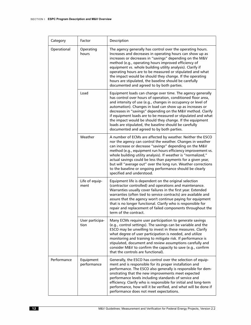
Operational Operating hours
The agency generally has control over the operating hours. Increases and decreases in operating hours can show up as increases or decreases in “savings” depending on the M&V method (e.g., operating hours improved efficiency ofequipment vs. whole building utility analysis). Clarify ifoperating hours are to be measured or stipulated and what the impact would be should they change. If the operating hours are stipulated, the baseline should be carefullydocumented and agreed to by both parties.
Load Equipment loads can change over time. The agency generally has control over hours of operation, conditioned floor area, and intensity of use (e.g., changes in occupancy or level of automation). Changes in load can show up as increases or decreases in “savings” depending on the M&V method. Clarify if equipment loads are to be measured or stipulated and what the impact would be should they change. If the equipment loads are stipulated, the baseline should be carefullydocumented and agreed to by both parties.
Weather A number of ECMs are affected by weather. Neither the ESCO nor the agency can control the weather. Changes in weather can increase or decrease “savings” depending on the M&V method (e.g., equipment run hours efficiency improvement vs. whole building utility analysis). If weather is “normalized,” actual savings could be less than payments for a given year, but will “average out” over the long run. Weather corrections to the baseline or ongoing performance should be clearly specified and understood.
Life of equip-ment
Equipment life is dependent on the original selection(contractor controlled) and operations and maintenance.Warranties usually cover failures in the first year. Extended warranties (often tied to service contracts) are available and assure that the agency won't continue paying for equipment that is no longer functional. Clarify who is responsible for repair and replacement of failed components throughout the term of the contract.
User participa-tion
Many ECMs require user participation to generate savings (e.g., control settings). The savings can be variable and the ESCO may be unwilling to invest in these measures. Clarify what degree of user participation is needed, and utilizemonitoring and training to mitigate risk. If performance is stipulated, document and review assumptions carefully and consider M&V to confirm the capacity to save (e.g., confirm that the controls are functional).
Performance Equipment performance
Generally, the ESCO has control over the selection of equip-ment and is responsible for its proper installation andperformance. The ESCO also generally is responsible for dem-onstrating that the new improvements meet expectedperformance levels including standards of service andefficiency. Clarify who is responsible for initial and long-term performance, how will it be verified, and what will be done if performance does not meet expectations.
Category Factor Description
M&V Guidelines: Measurement and Verification for Federal Energy Projects, Version 2.212
CHAPTER 2
Measurement and Verification: an Overview
2.2.2 Measurement and Verification PlanThe M&V plan is a document that defines project-specific measurement andverification methods for determining the savings resulting from performancecontracting projects. The plan may include a single option that addresses all the measures installed at a single facility or it may include several M&V options to address multiple measures installed at the facility. The ESCO prepares the project-specific M&V plan and submits it to the federal agency for review and approval.
The following material defines the general requirements for submitting a project-specific M&V plan. Issues and requirements associated with measure-specific M&V methods are described in Chapters 6–31. An overview of M&V plan contentrequirements and review procedures are provided in Chapter 5.
The steps, which can be iterative, for defining a project-specific M&V plan include the following:
• Identify goals and objectives.
• Specify the characteristics of the facility and the ECM or system to be installed.
• Specify by measure the M&V option, methods, and techniques to be used.
• Specify data analysis procedures, algorithms, assumptions, data requirements, and data products.
• Specify the metering points, period of metering, and analysis and meteringprotocols.
• Specify accuracy and quality assurance procedures.
• Specify the annual M&V report format and how results will be documented.
• Define budget and resource requirements.
It is important to realistically anticipate the costs and level of effort associated with completing metering and data analysis activities. Time and budget requirements are often underestimated. Note that metering is just one part of a successful M&Vprogram. Other key components include:
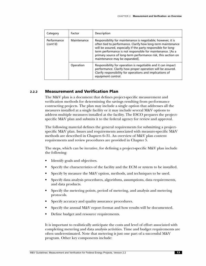
Performance (cont’d)
Maintenance Responsibility for maintenance is negotiable; however, it is often tied to performance. Clarify how long-term maintenance will be assured, especially if the party responsible for long-term performance is not responsible for maintenance. [As a primary source of long-term performance risk, this section on maintenance may be expanded].
Operation Responsibility for operation is negotiable and it can impact performance. Clarify how proper operation will be assured. Clarify responsibility for operations and implications ofequipment control.
Category Factor Description
M&V Guidelines: Measurement and Verification for Federal Energy Projects, Version 2.2 13
SECTION I
ESPC Program Description and M&V Overview
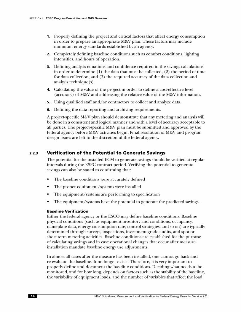
1. Properly defining the project and critical factors that affect energy consumption in order to prepare an appropriate M&V plan. These factors may includeminimum energy standards established by an agency.
2. Completely defining baseline conditions such as comfort conditions, lighting intensities, and hours of operation.
3. Defining analysis equations and confidence required in the savings calculations in order to determine (1) the data that must be collected, (2) the period of time for data collection, and (3) the required accuracy of the data collection andanalysis technique(s).
4. Calculating the value of the project in order to define a cost-effective level(accuracy) of M&V and addressing the relative value of the M&V information.
5. Using qualified staff and/or contractors to collect and analyze data.
6. Defining the data reporting and archiving requirements.
A project-specific M&V plan should demonstrate that any metering and analysis will be done in a consistent and logical manner and with a level of accuracy acceptable to all parties. The project-specific M&V plan must be submitted and approved by the federal agency before M&V activities begin. Final resolution of M&V and program design issues are left to the discretion of the federal agency.
2.2.3 Verification of the Potential to Generate SavingsThe potential for the installed ECM to generate savings should be verified at regular intervals during the ESPC contract period. Verifying the potential to generatesavings can also be stated as confirming that:
• The baseline conditions were accurately defined
• The proper equipment/systems were installed
• The equipment/systems are performing to specification
• The equipment/systems have the potential to generate the predicted savings.
Baseline VerificationEither the federal agency or the ESCO may define baseline conditions. Baseline physical conditions (such as equipment inventory and conditions, occupancy,nameplate data, energy consumption rate, control strategies, and so on) are typically determined through surveys, inspections, investment-grade audits, and spot orshort-term metering activities. Baseline conditions are established for the purposeof calculating savings and in case operational changes that occur after measure installation mandate baseline energy use adjustments.
In almost all cases after the measure has been installed, one cannot go back andre-evaluate the baseline. It no longer exists! Therefore, it is very important toproperly define and document the baseline conditions. Deciding what needs to bemonitored, and for how long, depends on factors such as the stability of the baseline, the variability of equipment loads, and the number of variables that affect the load.
M&V Guidelines: Measurement and Verification for Federal Energy Projects, Version 2.214
CHAPTER 2
Measurement and Verification: an Overview
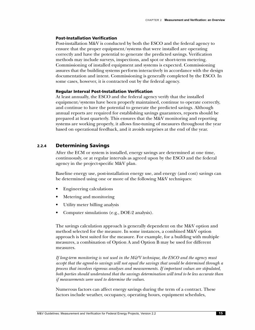
Post-Installation VerificationPost-installation M&V is conducted by both the ESCO and the federal agency to ensure that the proper equipment/systems that were installed are operatingcorrectly and have the potential to generate the predicted savings. Verificationmethods may include surveys, inspections, and spot or short-term metering.Commissioning of installed equipment and systems is expected. Commissioning assures that the building systems perform interactively in accordance with the design documentation and intent. Commissioning is generally completed by the ESCO. In some cases, however, it is contracted out by the federal agency.
Regular Interval Post-Installation VerificationAt least annually, the ESCO and the federal agency verify that the installedequipment/systems have been properly maintained, continue to operate correctly, and continue to have the potential to generate the predicted savings. Although annual reports are required for establishing savings guarantees, reports should be prepared at least quarterly. This ensures that the M&V monitoring and reportingsystems are working properly, it allows fine-tuning of measures throughout the year based on operational feedback, and it avoids surprises at the end of the year.
2.2.4 Determining SavingsAfter the ECM or system is installed, energy savings are determined at one time,continuously, or at regular intervals as agreed upon by the ESCO and the federal agency in the project-specific M&V plan.
Baseline energy use, post-installation energy use, and energy (and cost) savings can be determined using one or more of the following M&V techniques:
• Engineering calculations
• Metering and monitoring
• Utility meter billing analysis
• Computer simulations (e.g., DOE-2 analysis).
The savings calculation approach is generally dependent on the M&V option and method selected for the measure. In some instances, a combined M&V option approach is best suited for the measure. For example, for a building with multiple measures, a combination of Option A and Option B may be used for differentmeasures.
If long-term monitoring is not used in the M&V technique, the ESCO and the agency must accept that the agreed-to savings will not equal the savings that would be determined through a process that involves rigorous analyses and measurements. If important values are stipulated, both parties should understand that the savings determination will tend to be less accurate than if measurements were used to determine the values.
Numerous factors can affect energy savings during the term of a contract. Thesefactors include weather, occupancy, operating hours, equipment schedules,
M&V Guidelines: Measurement and Verification for Federal Energy Projects, Version 2.2 15

SECTION I
ESPC Program Description and M&V Overview
equipment maintenance, and equipment loads. The ESCO must submit as part of the M&V plan a description of how they will adjust the baseline if post-installation conditions are different than baseline conditions.
2.3 Measurement and Verification Options
This document contains measurement and verification guidelines grouped into four categories: Options A, B, C, and D. The options are generic M&V approaches for energy and water projects. Options A, B, C, and D are consistent with those defined in the 1998 International Performance Measurement and Verification Protocols (IPMVP). Having four options provides a range of approaches to determine energy savings with varying levels of uncertainty, cost, and methodology. A particular option is chosen based on the project-specific features of each ESPC. These features include the following:
• The complexity of the ECMs.
• The objective of the agency with respect to minimizing the risk of savings being achieved.
• The potential for changes in key factors between the baseline period and theperformance period.
• The measures' savings value.
The options differ in their approach to the level and duration of baseline andperformance period measurements. M&V evaluations for both options A and B are made at the retrofit or system level. Option C evaluations are made at the whole-building or whole-facility level. Option D evaluations, which involve computersimulation modeling, are made at either the retrofit or the whole-building level (for model calibration purposes).
Option A involves using stipulated and measured values of key factors needed to determine energy savings. Options B and C involve using spot, short-term, andcontinuous measurements. Option D may include spot, short-term, or continuous measurements to calibrate the model.
Options A and B activities specifically determine retrofit-level performance and operation factors. Performance refers to equipment and system efficiencycharacteristics such as kW/ton for chillers or watts/fixture for lighting. Operation refers to equipment and system operating characteristics such as annual coolington-hours for chillers or operating hours for lighting. Option C performance factors are determined at the whole-building or facility level. Option C operational factors are determined by utility meter or sub-metered data. Option D performance and operational factors are modeled based on design specifications. Measurements can be used to verify input values and calibrate the model.
The four generic M&V options are summarized in Table 2.2 and described in more detail below. Each option has advantages and disadvantages based on site-specific
M&V Guidelines: Measurement and Verification for Federal Energy Projects, Version 2.216
CHAPTER 2
Measurement and Verification: an Overview
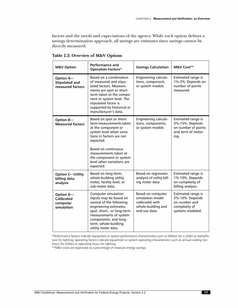
factors and the needs and expectations of the agency. While each option defines a savings determination approach, all savings are estimates since savings cannot be directly measured.
Table 2.2: Overview of M&V Options
*Performance factors indicate equipment or system performance characteristics such as kW/ton for a chiller or watts/fix-ture for lighting; operating factors indicate equipment or system operating characteristics such as annual cooling ton-hours for chillers or operating hours for lighting.**M&V costs are expressed as a percentage of measure energy savings.
M&V OptionPerformance and Operation Factors*
Savings Calculation M&V Cost**
Option A—Stipulated and measured factors
Based on a combination of measured and stipu-lated factors. Measure-ments are spot or short-term taken at the compo-nent or system level. The stipulated factor issupported by historical or manufacturer’s data.
Engineering calcula-tions, component, or system models.
Estimated range is 1%-3%. Depends on number of points measured.
Option B—Measured factors
Based on spot or short-term measurements taken at the component orsystem level when varia-tions in factors are not expected.
Based on continuous measurements taken at the component or system level when variations are expected.
Engineering calcula-tions, components, or system models.
Estimated range is 3%-15%. Depends on number of points and term of meter-ing.
Option C—Utility billing data analysis
Based on long-term, whole-building utility meter, facility level, or sub-meter data.
Based on regression analysis of utility bill-ing meter data.
Estimated range is 1%-10%. Depends on complexity of billing analysis.
Option D—Calibrated computer simulation
Computer simulation inputs may be based on several of the following: engineering estimates; spot, short-, or long-term measurements of system components; and long-term, whole-buildingutility meter data.
Based on computer simulation model calibrated with whole-building and end-use data.
Estimated range is 3%-10%. Depends on number and complexity ofsystems modeled.
M&V Guidelines: Measurement and Verification for Federal Energy Projects, Version 2.2 17
SECTION I
ESPC Program Description and M&V Overview
2.3.1 Option AAn Option A approach involves a retrofit or system level M&V assessment. The approach is intended for retrofits where either performance factors or operational factors can be spot or short-term measured during the baseline and post-installation periods. The factor not measured is stipulated based on assumptions, analysis ofhistorical data, or manufacturer's data. Using a stipulated factor is appropriate only if supporting data demonstrates that its value is not subject to fluctuation over the term of the contract
Option A focuses on the physical assessment of equipment change-outs to ensure the installation is to specification. The potential to generate savings may be verified through observation, inspections, and/or spot or short-term metering conducted immediately before and/or after installation. Inspections or spot or short-term metering may also be conducted at regular intervals to verify an ECM's or system's continued potential to generate savings.
With Option A, savings are determined by measuring the capacity, efficiency, or operation of a system before and after a retrofit and by multiplying the difference by a stipulated factor. Stipulation is the easiest and least expensive method ofdetermining savings. It can also be the least accurate and is typically the method with the greatest uncertainty of savings. This level of verification may suffice for certain types of projects in which a single factor represents a significant portion of thesavings uncertainty. Option A is appropriate for projects in which both parties agree to a payment stream that is not subject to fluctuation due to changes in theoperation or performance of the equipment (payments could be subject to change based on periodic measurements).
All end-use technologies can be verified using Option A; however, the accuracy of this option is generally inversely proportional to the complexity of the measure. In addition, within Option A, various methods and levels of accuracy in verifyingperformance/operation are available. The level of accuracy depends on the validity of assumptions, quality of the equipment inventory, and whether spot/short-term measurements are made. The penalty associated with low accuracy is not achieving the estimated measure savings and the associated utility bill cost reductions.
2.3.2 Option B Option B involves a retrofit or system-level M&V assessment. The approach is intended for retrofits with performance factors and operational factors that can be measured at the component or system level. It is appropriate to use spot or short-term measurements to determine energy savings when variations in operations are not expected to change. When variations are expected, it is appropriate to measure factors continuously during the contract. Continuous measurements provide long-term performance data on the energy use of the equipment or system. These data can be used to improve or optimize the operation of the equipment on a real-time basis, thereby improving the benefit of the retrofit.
Option B verification procedures involve the same items as Option A but generally involve more end-use metering. Option B relies on the physical assessment of
M&V Guidelines: Measurement and Verification for Federal Energy Projects, Version 2.218
CHAPTER 2
Measurement and Verification: an Overview
equipment change-outs to ensure the installation is to specification. The potential to generate savings is verified through observations, inspections, and spot, short-term, or continuous metering. The continuous metering of one or more variables may only occur after retrofit installation. Spot or short-term metering may be sufficient to characterize the baseline condition.
Option B relies on the direct measurement of end uses affected by the retrofit.Individual loads are monitored after ECM or system installation to determineperformance. This measured performance is compared with a baseline model, also based on measurements, to determine savings.
All end-use technologies can be verified with Option B; however, the degree ofdifficulty and costs associated with verification increases as metering complexity increases. The task of measuring or determining energy savings using Option B can be more difficult and costly than that of Option A. The results, however, are typically more accurate. The use of periodic or continuous measurement accounts foroperating variations. Spot or short-term measurements are sufficient for constant load retrofits. Using measurements more closely approximates actual energy savings than the use of stipulations as defined for Option A. Measurement of all end-use equipment or systems may not be required if statistically valid sampling is used. For example, the operating hours for a selected group of lighting fixtures or the power draw from a subset of representative constant-load motors may be metered.
2.3.3 Option C Verification techniques for Option C determine savings by studying overall energy use in a facility and identifying the impact of conservation measures on totalbuilding or facility energy use patterns. The evaluation of whole-building or facility-level metered data is completed using techniques ranging from simple billingcomparison to multivariate regression analysis. In general for federal ESPC projects, billing comparison methods are not recommended for estimating energy savings. Option C regression methods are valuable for measuring interactions between energy systems or determining the impact of projects that cannot be measured directly, such as insulation or other building envelope measures.
Option C involves procedures for verifying the potential to generate savings that are the same as Option A. Option C also involves determining energy savings during the contract term using whole-building metering data. Option C includes a physical assessment of equipment change-outs to ensure the installation is to specification. The potential to generate savings is verified through observation and inspection. The actual energy savings is determined from measured utility billing data and regression analysis modeling. All explanatory variables that affect energyconsumption need to be monitored during the term of the contract for use in the model. Critical variables may include weather, occupancy schedules, set points, and operating schedules. Option C usually requires at least 9 to 12 months of continuous data before a retrofit and continuous data after the retrofit. The data can be hourly or monthly whole-building data.
M&V Guidelines: Measurement and Verification for Federal Energy Projects, Version 2.2 19
SECTION I ESPC Program Description and M&V Overview
All end-use technologies can be verified with Option C, provided that the reduction in consumption is larger than the associated modeling error. This option may be used in cases in which there is a high degree of interaction between installed energy conservation systems and/or the measurement of individual component savings is not cost-effective. Accounting for changes (other than those caused by theconservation measures) is the major challenge associated with Option C, particularly for long-term contracts.
2.3.4 Option DOption D involves calibrated computer simulation models of component or whole-building energy consumption to determine measure energy savings. Linkingsimulation inputs to baseline and post-installation conditions completes thecalibration. Characterizing baseline and post-installation conditions may involve metering performance and operating factors before and after the retrofit. Long-term whole-building energy use data may be used to calibrate the simulation(s).
Option D involves procedures for verifying the potential to generate savings that are the same as Option A. Option D also involves determining energy savings during the contract term through the use of a calibrated simulation analysis. Option D includes a physical assessment of equipment change-outs to ensure the installation is tospecification. The potential to generate savings is verified through observation, inspection, and measurements. Manufacturer's data, spot measurements, or short-term measurements may be used to characterize baseline and post-installationconditions and operating schedules. The data serve to link the simulation inputs to actual operating conditions. The model calibration is accomplished by comparing simulation results with end-use or whole-building data. For whole-building models, option D usually requires at least 9 to 12 months of data before and after the retrofit. If continuous, post-installation data are used, the simulation model can be calibrated at regular intervals to update the savings estimates.
All end-use technologies can be verified with Option D, provided that the size of the drop in consumption is larger than the associated modeling error. This option may be used in cases where there is a high degree of interaction among installed energy conservation systems and/or the measurement of individual component savings is difficult. Accurate modeling and calibration are the major challenges associated with Option D. The building simulation model may involve elaborate models (such as DOE-2), spreadsheets, or vendor estimating programs. More elaborate models may improve accuracy and increase modeling costs.
2.4 M&V Methods
An M&V method is a measure-specific M&V approach based on one of the four M&V options. The M&V Guidelines present methods for determining energy savings for common ECMs. All of the methods for determining energy savings are based on the same concept: savings are derived by comparing usage after the retrofit to what the usage would have been without the retrofit (i.e., the baseline). The federal agency
M&V Guidelines: Measurement and Verification for Federal Energy Projects, Version 2.220
CHAPTER 2 Measurement and Verification: an Overview
and the ESCO will select an M&V option and method for each project and thenprepare a site-specific M&V plan that incorporates project-specific details, asdiscussed in this document.
Thus far, the Guidelines have focused on the generic M&V categories of Options A, B, C, and D, as defined in the IPMVP. This section summarizes the M&V methods, categorized by option and ECM technology, provided in this document. The ECMs covered are those that are most commonly implemented though performancecontracts.
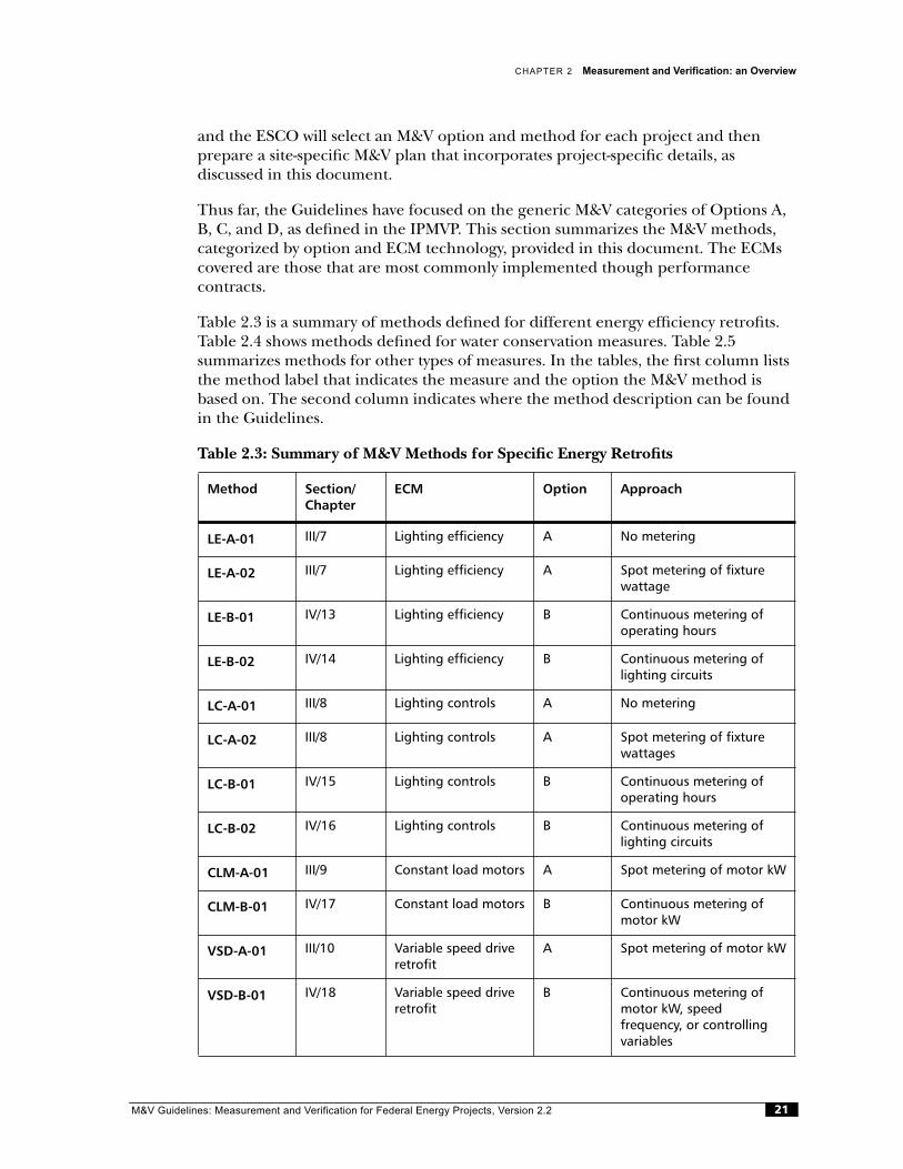
Table 2.3 is a summary of methods defined for different energy efficiency retrofits. Table 2.4 shows methods defined for water conservation measures. Table 2.5summarizes methods for other types of measures. In the tables, the first column lists the method label that indicates the measure and the option the M&V method is based on. The second column indicates where the method description can be found in the Guidelines.
Table 2.3: Summary of M&V Methods for Specific Energy Retrofits
Method Section/Chapter
ECM Option Approach
LE-A-01 III/7 Lighting efficiency A No metering
LE-A-02 III/7 Lighting efficiency A Spot metering of fixture wattage
LE-B-01 IV/13 Lighting efficiency B Continuous metering of operating hours
LE-B-02 IV/14 Lighting efficiency B Continuous metering of lighting circuits
LC-A-01 III/8 Lighting controls A No metering
LC-A-02 III/8 Lighting controls A Spot metering of fixture wattages
LC-B-01 IV/15 Lighting controls B Continuous metering of operating hours
LC-B-02 IV/16 Lighting controls B Continuous metering of lighting circuits
CLM-A-01 III/9 Constant load motors A Spot metering of motor kW
CLM-B-01 IV/17 Constant load motors B Continuous metering of motor kW
VSD-A-01 III/10 Variable speed drive retrofit
A Spot metering of motor kW
VSD-B-01 IV/18 Variable speed drive retrofit
B Continuous metering of motor kW, speedfrequency, or controlling variables
M&V Guidelines: Measurement and Verification for Federal Energy Projects, Version 2.2 21
SECTION I ESPC Program Description and M&V Overview
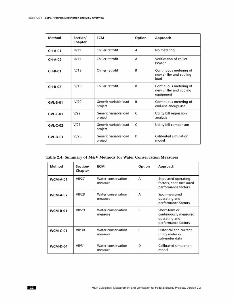
Table 2.4: Summary of M&V Methods for Water Conservation Measures
CH-A-01 III/11 Chiller retrofit A No metering
CH-A-02 III/11 Chiller retrofit A Verification of chillerkW/ton
CH-B-01 IV/19 Chiller retrofit B Continuous metering of new chiller and cooling load
CH-B-02 IV/19 Chiller retrofit B Continuous metering of new chiller and cooling equipment
GVL-B-01 IV/20 Generic variable load project
B Continuous metering of end-use energy use
GVL-C-01 V/22 Generic variable load project
C Utility bill regressionanalysis
GVL-C-02 V/23 Generic variable load project
C Utility bill comparison
GVL-D-01 VI/25 Generic variable load project
D Calibrated simulation model
Method Section/Chapter
ECM Option Approach
WCM-A-01 VII/27 Water conservation measure
A Stipulated operating factors, spot-measured performance factors
WCM-A-02 VII/28 Water conservation measure
A Spot-measuredoperating andperformance factors
WCM-B-01 VII/29 Water conservation measure
B Short-term orcontinuously measured operating andperformance factors
WCM-C-01 VII/30 Water conservation measure
C Historical and current utility meter orsub-meter data
WCM-D-01 VII/31 Water conservation measure
D Calibrated simulation model
Method Section/Chapter
ECM Option Approach
M&V Guidelines: Measurement and Verification for Federal Energy Projects, Version 2.222
CHAPTER 2 Measurement and Verification: an Overview
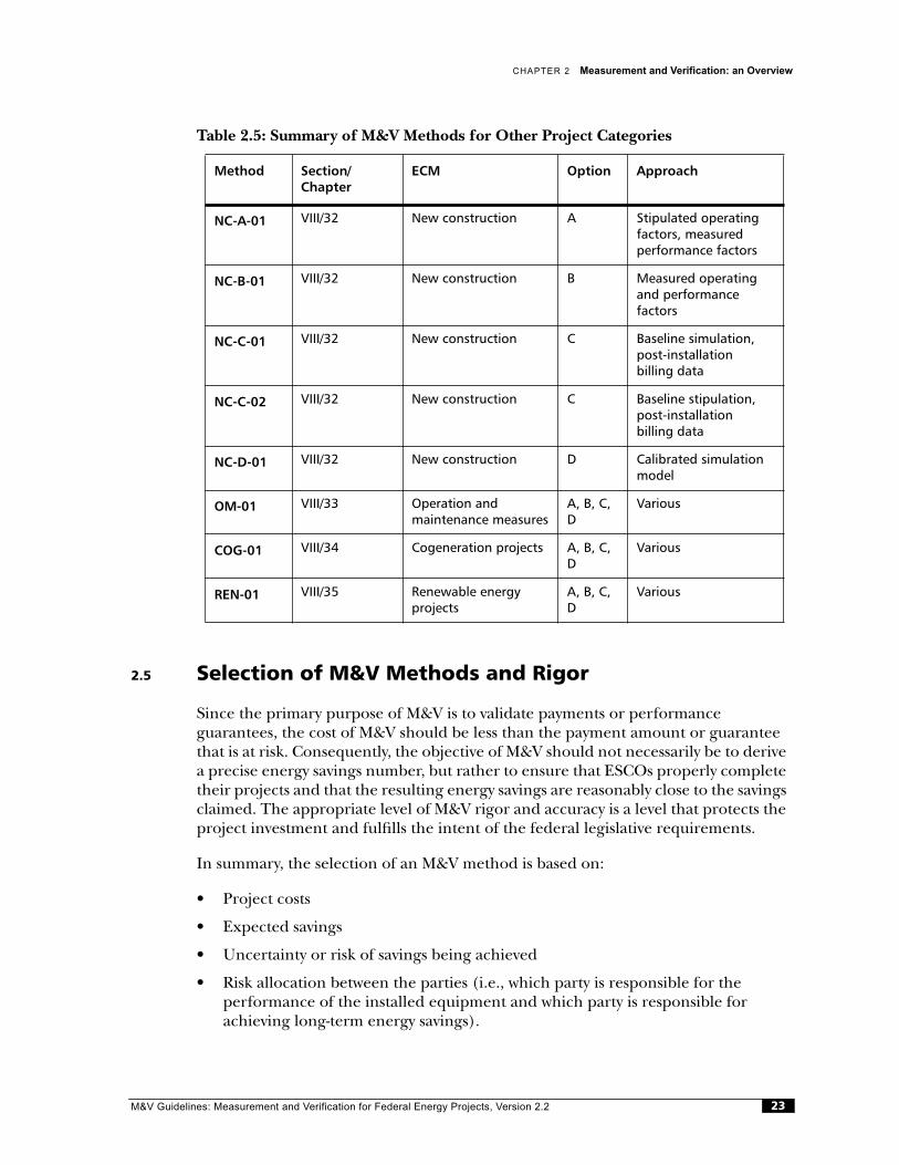
Table 2.5: Summary of M&V Methods for Other Project Categories
2.5 Selection of M&V Methods and Rigor
Since the primary purpose of M&V is to validate payments or performanceguarantees, the cost of M&V should be less than the payment amount or guarantee that is at risk. Consequently, the objective of M&V should not necessarily be to derive a precise energy savings number, but rather to ensure that ESCOs properly complete their projects and that the resulting energy savings are reasonably close to the savings claimed. The appropriate level of M&V rigor and accuracy is a level that protects the project investment and fulfills the intent of the federal legislative requirements.
In summary, the selection of an M&V method is based on:
• Project costs
• Expected savings
• Uncertainty or risk of savings being achieved
• Risk allocation between the parties (i.e., which party is responsible for theperformance of the installed equipment and which party is responsible for achieving long-term energy savings).
Method Section/Chapter
ECM Option Approach
NC-A-01 VIII/32 New construction A Stipulated operating factors, measuredperformance factors
NC-B-01 VIII/32 New construction B Measured operating and performancefactors
NC-C-01 VIII/32 New construction C Baseline simulation, post-installationbilling data
NC-C-02 VIII/32 New construction C Baseline stipulation, post-installationbilling data
NC-D-01 VIII/32 New construction D Calibrated simulation model
OM-01 VIII/33 Operation andmaintenance measures
A, B, C, D
Various
COG-01 VIII/34 Cogeneration projects A, B, C, D
Various
REN-01 VIII/35 Renewable energy projects
A, B, C, D
Various
M&V Guidelines: Measurement and Verification for Federal Energy Projects, Version 2.2 23
SECTION I ESPC Program Description and M&V Overview
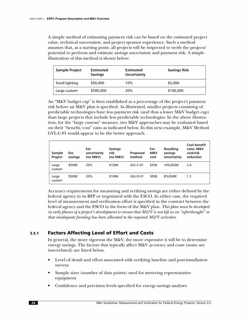
A simple method of estimating payment risk can be based on the estimated project value, technical uncertainty, and project sponsor experience. Such a method assumes that, as a starting point, all projects will be inspected to verify the projects’ potential to perform and estimate savings uncertainty and payment risk. A simple illustration of this method is shown below:
An “M&V budget cap” is then established as a percentage of the project's payment risk before an M&V plan is specified. As illustrated, smaller projects consisting ofpredictable technologies have less payment risk (and thus a lower M&V budget cap) than large projects that include less predictable technologies. In the above illustra-tion, for the “large custom” measure, two M&V approaches may be evaluated based on their “benefit/cost” ratio as indicated below. In this next example, M&V Method GVL-C-01 would appear to be the better approach.
Accuracy requirements for measuring and verifying savings are either defined by the federal agency in its RFP or negotiated with the ESCO. In either case, the required level of measurement and verification effort is specified in the contract between the federal agency and the ESCO in the form of the M&V plan. This plan must be developed in early phases of a project's development to ensure that M&V is not left as an “afterthought” or that inadequate funding has been allocated to the required M&V activities.
2.5.1 Factors Affecting Level of Effort and CostsIn general, the more rigorous the M&V, the more expensive it will be to determine energy savings. The factors that typically affect M&V accuracy and costs (some are interrelated) are listed below.
• Level of detail and effort associated with verifying baseline and post-installation surveys
• Sample sizes (number of data points) used for metering representativeequipment
• Confidence and precision levels specified for energy savings analyses
Sample Project Estimated Savings
Estimated Uncertainty
Savings Risk
Small lighting $50,000 10% $5,000
Large custom $500,000 20% $100,000
Sample Project
Est. savings
Est. uncertainty (no M&V)
Savings risk (no M&V)
Proposed method
Est. M&V cost
Resulting savings uncertainty
Cost benefit ratio: M&V cost/risk reduction
Large custom
$500K 20% $100K GVL-C-01 $25K 10%/$50K 2.0
Large custom
$500K 20% $100K GVL-D-01 $50K 8%/$40K 1.2
M&V Guidelines: Measurement and Verification for Federal Energy Projects, Version 2.224

CHAPTER 2 Measurement and Verification: an Overview
• Duration and accuracy of metering activities
• Number and complexity of dependent and independent variables that are metered or accounted for in analyses
• Availability of existing data collecting systems (e.g., energy management systems)
• Contract term.
2.5.2 Selecting the Appropriate M&V Option and MethodAs noted, the level of certainty and effort required to verify both a project's potential to perform and its actual performance will vary from project to project. The draft RFP, the actual contract, and/or the project-specific M&V plan should be prepared with serious consideration of what M&V requirements, reviews, and costs will be specified.
These are some factors that affect the decision of which M&V option, method, and technique to use for each ESPC project:
Value of ECM in Terms of Projected SavingsThe scale of a project, energy rates, term of the contract, comprehensiveness of ECMs, the benefit-sharing arrangement, and the magnitude of savings can all affect the value of the ESPC project. The M&V effort should be scaled to the value of the project so that the value of the information provided by the M&V activity isappropriate to the value of the project itself. “Rule of thumb” estimates put M&V costs at 1% to 10% of typical project cost savings.
Complexity of ECM or SystemMore complex projects may require more complex (and thus more expensive) M&V methods to determine energy savings. In general, the complexity of isolating thesavings is the critical factor. For example, a complicated HVAC measure may not be difficult to assess if there is a utility meter dedicated to the HVAC system.
When defining the appropriate M&V requirements for a given project, it is helpful to consider projects as being in one of the following categories (listed in order of increasing M&V complexity):
• Constant load, constant operating hours
• Constant load, variable operating hours
– Variable hours with a fixed pattern
– Variable hours without a fixed pattern (e.g., weather-dependent)
• Variable load, variable operating hours
– Variable hours or load with a fixed pattern
– Variable hours or load without a fixed pattern (e.g., weather-dependent).
M&V Guidelines: Measurement and Verification for Federal Energy Projects, Version 2.2 25
SECTION I ESPC Program Description and M&V Overview
Number of Interrelated ECMs at a Single FacilityIf multiple ECMs are being installed at a single site, the savings from each measure may be, to some degree, related to the savings resulting from other measure(s) or other non-ECM activities at the facility. Examples include interactive effects between lighting and HVAC measures or between HVAC control measures and a chiller replacement. In these situations, it is probably not possible to isolate and measure one system in order to determine savings. Thus, for multiple, interrelated measures, Option C is almost always required.
Uncertainty of SavingsThe importance of the M&V activities is often tied to the uncertainty associated with the estimated energy or cost savings. An ECM with which the facility staff is familiar may, subjectively, require less M&V rigor than ECMs that are less well known. Inaddition, if the ECM is similar to other projects that have been completed, and for which savings have been documented, the M&V results may be applied from the other project. If the ESCO specifies the baseline, it may be more appropriate to use M&V Options B or C to verify savings.
Responsibility (or Risk) Allocation between the ESCO and the Federal AgencyIf an ESCO's payments are not tied to actual savings, M&V activities are not required. Likewise, if an ESCO is not held responsible for certain aspects of a project'sperformance, these aspects do not need to be measured or verified. Theresponsibility matrix and contract should specify how payments will be determined and thus what needs to be verified. For example, variations in the operating hours of a facility during the term of a contract may be a risk the federal agency takes. Also, operating hours may be determined by short-term and not continuousmeasurements for purposes of payment, in which case Option A may be appropriate.
Other Uses for M&V Data and SystemsOften, the array of instrumentation installed and the measurements collected for M&V can be used for other purposes, including commissioning and systemoptimization. Data and systems are more cost-effective if they are used to meetseveral objectives, and not just those of the M&V plan. In addition, savings could be quantified beyond the requirements of the performance contract. This information could be useful for allocating costs among different tenants, planning future projects, or allocating research.
2.5.3 Criteria for Selecting an M&V ApproachThe four M&V options can be applied to almost any type of ECM; however, the rules-of-thumb listed below generally indicate the most appropriate M&V approach for an application.
Option A can be applied when identifying the potential to generate savings is the most critical M&V issue, including situations in which:
• The magnitude of savings is low for the entire project or a portion of the project to which Option A can be applied.
M&V Guidelines: Measurement and Verification for Federal Energy Projects, Version 2.226
CHAPTER 2 Measurement and Verification: an Overview
• The risk of achieving savings is low or ESCO payments are not directly tied to actual savings.
Option B, retrofit isolation, is typically used when any or all of these conditions apply:
• For simple equipment replacement projects with energy savings that are less than 20% of total facility energy use as recorded by the relevant utility meter orsub-meter.
• Energy savings values per individual measure are desired.
• Interactive effects are to be ignored or are stipulated using estimating methods that do not involve long-term measurements.
• The independent variables that affect energy use are neither complex norexcessively difficult or expensive to monitor.
• Sub-meters already exist that record the energy use of subsystems underconsideration (e.g., a 277 Volt lighting circuit or a separate sub-meter forHVAC systems).
Option C, billing analysis, is typically used when any or all of these conditions apply:
• The equipment replacement and controls projects are complex.
• Predicted savings are relatively large (greater than 10% to 20%) as compared to the energy use recorded by the relevant utility meter or sub-meter.
• Energy savings values per individual measure are not desired.
• Interactive effects are to be included.
• Independent variables that affect energy use are not complex and excessivelydifficult or expensive to monitor.
Option D, calibrated simulation, is used in situations similar to Option C, or inaddition when any or all of these conditions apply:
• New construction projects are involved.
• Energy savings values per measure are desired.
• Option C tools cannot cost effectively evaluate particular measures or theirinteractions with the building when complex baseline adjustments areanticipated.
2.5.4 Measure-Specific M&V Methods and ResponsibilitiesThe M&V methods summarized in this section are organized by ECM and M&V option. For each measure, a table highlights the components of several M&Vmethods. The measures included are lighting efficiency (LE), lighting controls (LC), efficient constant load motors (CLM), variable-speed drive (VSD)
M&V Guidelines: Measurement and Verification for Federal Energy Projects, Version 2.2 27

SECTION I ESPC Program Description and M&V Overview
installations, and chiller (CH) replacements. Tables 2.6–2.10 summarize themeasure-specific M&V approaches, which are methods based on Options A or B.The ESCO and agency responsibilities and risks associated with each method are outlined in the tables.
As described previously, variable load/variable operating hour projects require more rigorous M&V than constant load/constant operating hour projects. The lighting efficiency and constant load motor measures are representative of constant load, constant operating hour projects. The lighting control measures are representative of constant load, variable operating projects. The variable-speed drive and chiller replacements are representative of variable load, variable operating hour projects.
For more details about developing M&V plans for these M&V methods, refer toSection III, Chapters 6–11 for Option A-based approaches; to Section IV, Chapters 12 - 20 for Option B-based approaches; to Section V, Chapters 21–23 for OptionC-based approaches; and to Section VI, Chapters 24–25 for Option D-based approaches.
M&V Guidelines: Measurement and Verification for Federal Energy Projects, Version 2.228
CHAPTER 2 Measurement and Verification: an Overview
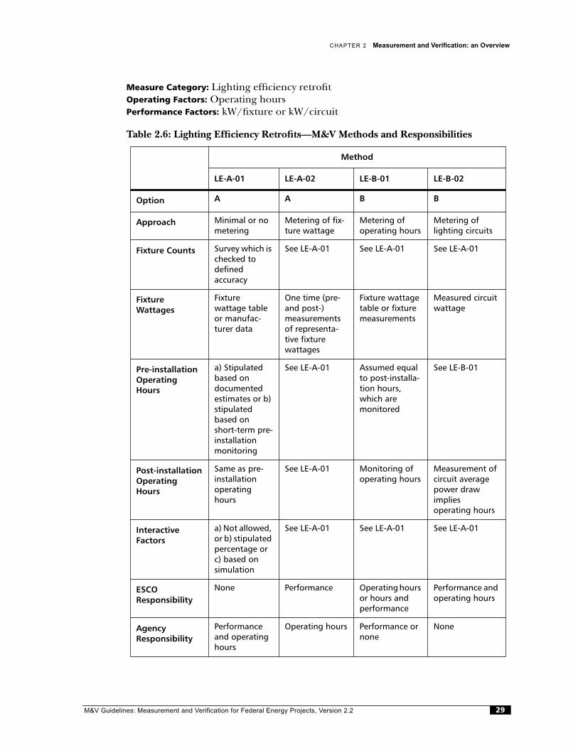
Measure Category: Lighting efficiency retrofitOperating Factors: Operating hoursPerformance Factors: kW/fixture or kW/circuit
Table 2.6: Lighting Efficiency Retrofits—M&V Methods and Responsibilities
Method
LE-A-01 LE-A-02 LE-B-01 LE-B-02
Option A A B B
Approach Minimal or no metering
Metering of fix-ture wattage
Metering of operating hours
Metering of lighting circuits
Fixture Counts Survey which is checked to definedaccuracy
See LE-A-01 See LE-A-01 See LE-A-01
Fixture Wattages
Fixturewattage table or manufac-turer data
One time (pre-and post-)measurements of representa-tive fixture wattages
Fixture wattage table or fixture measurements
Measured circuit wattage
Pre-installation Operating Hours
a) Stipulated based ondocumented estimates or b) stipulated based on short-term pre-installation monitoring
See LE-A-01 Assumed equal to post-installa-tion hours, which aremonitored
See LE-B-01
Post-installation Operating Hours
Same as pre-installation operating hours
See LE-A-01 Monitoring of operating hours
Measurement of circuit average power draw impliesoperating hours
Interactive Factors
a) Not allowed, or b) stipulated percentage or c) based on simulation
See LE-A-01 See LE-A-01 See LE-A-01
ESCO Responsibility
None Performance Operating hours or hours and performance
Performance and operating hours
Agency Responsibility
Performance and operating hours
Operating hours Performance or none
None
M&V Guidelines: Measurement and Verification for Federal Energy Projects, Version 2.2 29

SECTION I ESPC Program Description and M&V Overview
Measure Category: Lighting controls retrofitsOperating Factors: Operating hoursPerformance Factors: kW/fixture or kW/circuit
Table 2.7: Lighting Controls Retrofits—M&V Methods and Responsibilities
Method
LC-A-01 LC-A-02 LC-B-01 LC-B-02
Option A A B B
Approach Minimal or no metering
Metering of fixture wattages
Metering of operating hours
Metering of lighting circuits
Fixture Counts Survey which is checked to definedaccuracy
See LC-A-01 See LC-A-01 See LC-A-01
Fixture Wattages
Fixture or watt-age table or manufacturer data
One time mea-surements of representative fixture wattages
Fixture wattage table or one time fixture measurements
Measured circuit wattage
Pre-installation Operating Hours
a) Stipulated based on esti-mates or b) stipulated based on short-term pre-install monitor-ing
See LC-A-01 Operating hours are monitored for representa-tive samples of fixtures
The circuitmeasurement of average power draw alsoprovidesoperating hours
Post-installation Operating Hours
a) Stipulated based onestimates or b) stipulated based on short-term post-install monitoring
See LC-A-01 Operating hours are monitored for representa-tive samples of fixtures
The circuitmeasurement of average power draw alsoprovidesoperating hours
Interactive Factors
a) Not allowed, or b) stipulated percentage, or c) based on simulation
See LC-A-01 See LC-A-01 See LC-A-01
ESCO Responsibility
None Performance Operating hours or hours and performance
Performance and operating hours
Agency Responsibility
Performance and operating hours
Operating hours Performance or none
None
M&V Guidelines: Measurement and Verification for Federal Energy Projects, Version 2.230
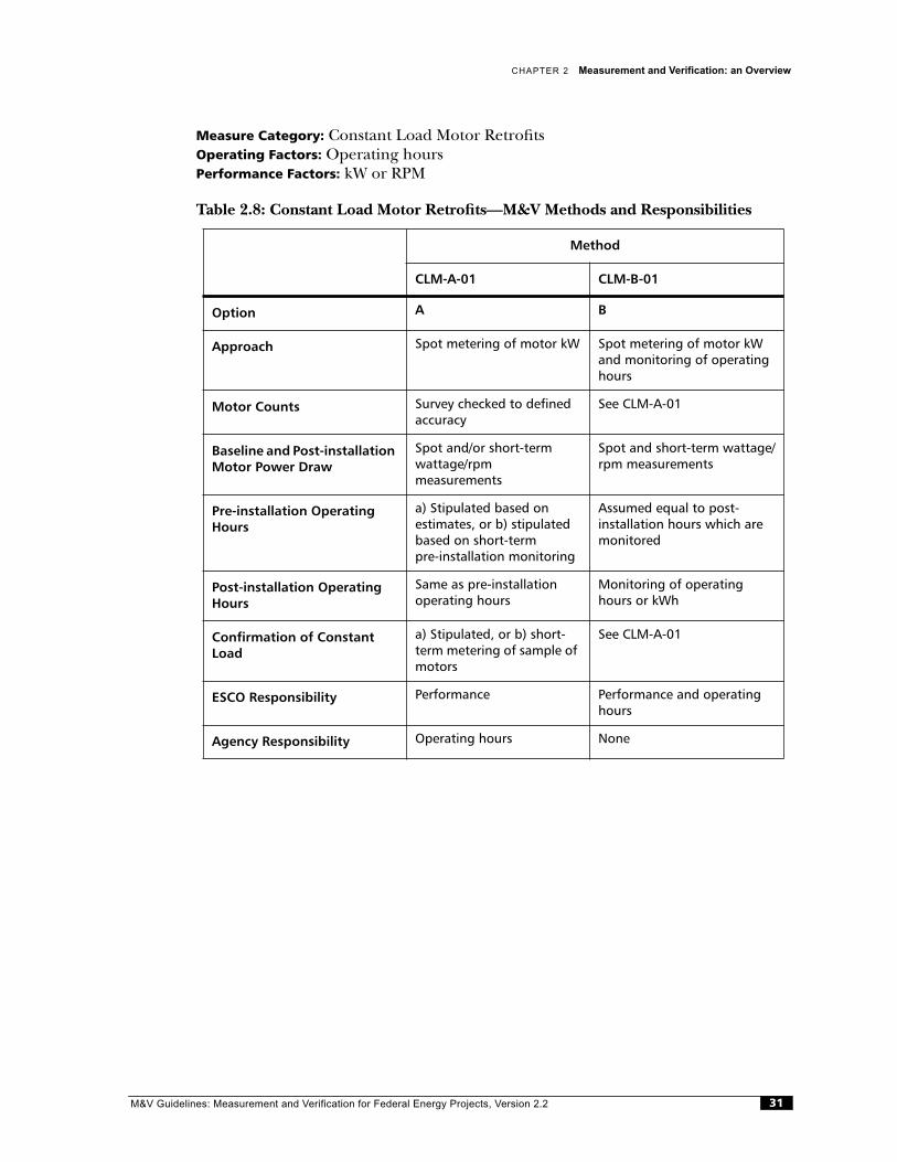
CHAPTER 2 Measurement and Verification: an Overview
Measure Category: Constant Load Motor RetrofitsOperating Factors: Operating hoursPerformance Factors: kW or RPM
Table 2.8: Constant Load Motor Retrofits—M&V Methods and Responsibilities
Method
CLM-A-01 CLM-B-01
Option A B
Approach Spot metering of motor kW Spot metering of motor kW and monitoring of operating hours
Motor Counts Survey checked to defined accuracy
See CLM-A-01
Baseline and Post-installation Motor Power Draw
Spot and/or short-term wattage/rpmmeasurements
Spot and short-term wattage/rpm measurements
Pre-installation Operating Hours
a) Stipulated based onestimates, or b) stipulated based on short-termpre-installation monitoring
Assumed equal to post-installation hours which are monitored
Post-installation Operating Hours
Same as pre-installation operating hours
Monitoring of operating hours or kWh
Confirmation of Constant Load
a) Stipulated, or b) short-term metering of sample of motors
See CLM-A-01
ESCO Responsibility Performance Performance and operating hours
Agency Responsibility Operating hours None
M&V Guidelines: Measurement and Verification for Federal Energy Projects, Version 2.2 31
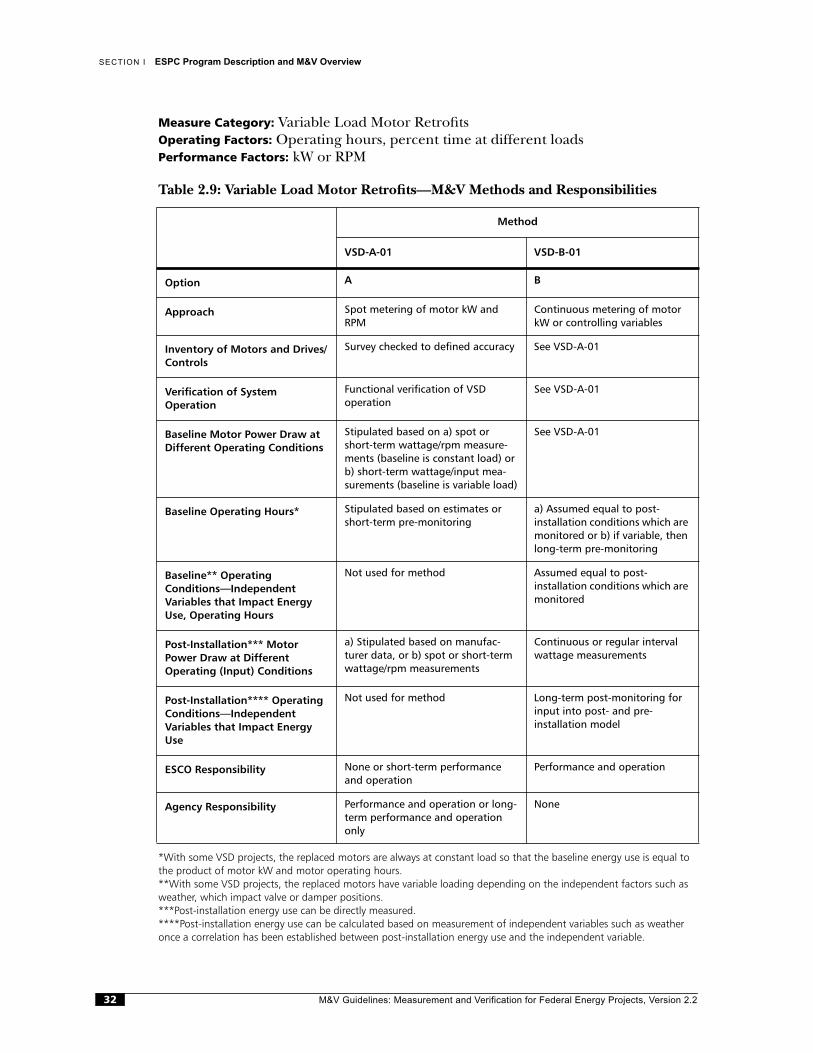
SECTION I ESPC Program Description and M&V Overview
Measure Category: Variable Load Motor RetrofitsOperating Factors: Operating hours, percent time at different loadsPerformance Factors: kW or RPM
Table 2.9: Variable Load Motor Retrofits—M&V Methods and Responsibilities
*With some VSD projects, the replaced motors are always at constant load so that the baseline energy use is equal to the product of motor kW and motor operating hours.**With some VSD projects, the replaced motors have variable loading depending on the independent factors such as weather, which impact valve or damper positions.***Post-installation energy use can be directly measured.****Post-installation energy use can be calculated based on measurement of independent variables such as weather once a correlation has been established between post-installation energy use and the independent variable.
Method
VSD-A-01 VSD-B-01
Option A B
Approach Spot metering of motor kW and RPM
Continuous metering of motor kW or controlling variables
Inventory of Motors and Drives/Controls
Survey checked to defined accuracy See VSD-A-01
Verification of System Operation
Functional verification of VSDoperation
See VSD-A-01
Baseline Motor Power Draw at Different Operating Conditions
Stipulated based on a) spot or short-term wattage/rpm measure-ments (baseline is constant load) or b) short-term wattage/input mea-surements (baseline is variable load)
See VSD-A-01
Baseline Operating Hours* Stipulated based on estimates or short-term pre-monitoring
a) Assumed equal to post-installation conditions which are monitored or b) if variable, then long-term pre-monitoring
Baseline** Operating Conditions—Independent Variables that Impact Energy Use, Operating Hours
Not used for method Assumed equal to post-installation conditions which are monitored
Post-Installation*** Motor Power Draw at Different Operating (Input) Conditions
a) Stipulated based on manufac-turer data, or b) spot or short-term wattage/rpm measurements
Continuous or regular interval wattage measurements
Post-Installation**** Operating Conditions—Independent Variables that Impact Energy Use
Not used for method Long-term post-monitoring for input into post- and pre-installation model
ESCO Responsibility None or short-term performance and operation
Performance and operation
Agency Responsibility Performance and operation or long-term performance and operation only
None
M&V Guidelines: Measurement and Verification for Federal Energy Projects, Version 2.232
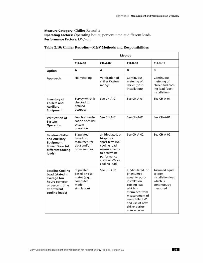
CHAPTER 2 Measurement and Verification: an Overview
Measure Category: Chiller RetrofitsOperating Factors: Operating hours, percent time at different loadsPerformance Factors: kW/ton
Table 2.10: Chiller Retrofits—M&V Methods and Responsibilities
Method
CH-A-01 CH-A-02 CH-B-01 CH-B-02
Option A A B B
Approach No metering Verification of chiller kW/ton ratings
Continuous metering of chiller (post-installation)
Continuous metering of chiller and cool-ing load (post-installation)
Inventory of Chillers and Auxiliary Equipment
Survey which is checked to definedaccuracy
See CH-A-01 See CH-A-01 See CH-A-01
Verification of System Operation
Function verifi-cation of chiller systemoperation
See CH-A-01 See CH-A-01 See CH-A-01
Baseline Chiller and Auxiliary Equipment Power Draw (at different cooling loads)
Stipulated based onmanufacturer data and/or other sources
a) Stipulated, or b) spot orshort-term kW/cooling load measurements to determine performance curve or kW vs. cooling load
See CH-A-02 See CH-A-02
Baseline Cooling Load (stated in average ton hours per year or percent time at different cooling loads)
Stipulated based on esti-mates (e.g., computer modelsimulation)
See CH-A-01 a) Stipulated, or b) assumed equal to post-installationcooling load which is etermined from measurement of new chiller kW and use of new chiller perfor-mance curve
Assumed equal to post-installation load which is continuously measured
M&V Guidelines: Measurement and Verification for Federal Energy Projects, Version 2.2 33
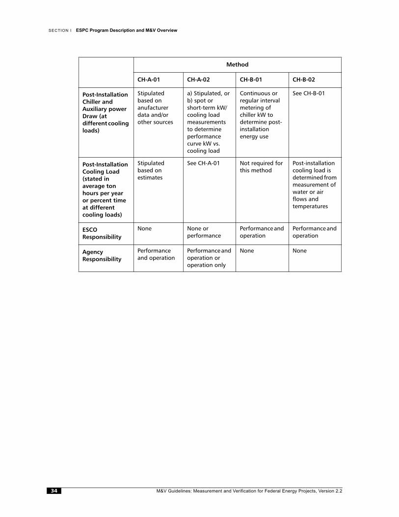
SECTION I ESPC Program Description and M&V Overview
Post-Installation Chiller and Auxiliary power Draw (at different cooling loads)
Stipulated based on anufacturer data and/or other sources
a) Stipulated, or b) spot orshort-term kW/cooling load measurements to determine performance curve kW vs. cooling load
Continuous or regular interval metering of chiller kW to determine post-installation energy use
See CH-B-01
Post-Installation Cooling Load (stated in average ton hours per year or percent time at different cooling loads)
Stipulated based on estimates
See CH-A-01 Not required for this method
Post-installation cooling load is determined from measurement of water or air flows andtemperatures
ESCO Responsibility
None None orperformance
Performance and operation
Performance and operation
Agency Responsibility
Performance and operation
Performance and operation or operation only
None None
Method
CH-A-01 CH-A-02 CH-B-01 CH-B-02
M&V Guidelines: Measurement and Verification for Federal Energy Projects, Version 2.234
M&V Guidelines:
Section II:Incorporating M&V into ESPCs
The three chapters in this section provide information on incorporatingM&V in a performance-based contract for energy or water conservationprojects. The procedures are also applicable to other types of projectsdiscussed in these Guidelines, such as those involving renewable energy,operations and maintenance measures, and cogeneration. The implemen-tation issues addressed include the project M&V procedural steps, thepreparation and assessment of the M&V plan, and M&V checklists. Thetitles of the three chapters in this section are:
• Chapter 3: Overview of M&V Procedural Steps and Submittals
• Chapter 4: M&V Plan Preparation and Assessment
• Chapter 5: M&V Quick-Start Guidelines
Measurement and Verification for Federal Energy Projects, Version 2.2 35
3Overview of M&V Procedural Steps and Submittals
This chapter is an overview of general M&V activities associated with implementing ESPC projects. The information is useful for preparing feasibility studies, requests for proposals (RFPs), performance contracts, and for documenting baselineconditions. The data and analyses performed during M&V development andbaseline characterization can be updated and used later in the project.
3.1 M&V Activities
M&V activities fall into the following five areas:
1. Define M&V requirements for inclusion in the contract between the federal agency and the ESCO based on the M&V options and methods defined in other sections of this document.
2. As soon as the project has been fully defined before the contract is signed,prepare a site-specific M&V plan for the project.
3. Define the pre-installation baseline, including (a) equipment and systems, (b) baseline energy use (and cost), and/or (c) factors that influence baseline energy use. The baseline can be defined through site surveys; spot, short-term, or long-term metering; and/or analysis of billing data. This activity may occur before or after the contract is signed.
4. Define the post-installation situation, including (a) equipment and systems, (b) post-installation energy use (and cost), and/or (c) factors that influence post-installation energy use. Site surveys; spot, short-term, or long-term metering; and/or analysis of billing data can be used for the post-installation assessment.
5. Conduct annual M&V activities to (a) verify the operation of the installedequipment/systems, (b) determine current year savings, and (c) estimate savings for subsequent years.
3.2 M&V Activity Details
As a contract is implemented, both the federal agency and ESCO take certain steps with respect to the measurement and verification of each project. Figure 3.1 presents a flow chart of those steps.
M&V Guidelines: Measurement and Verification for Federal Energy Projects, Version 2.236
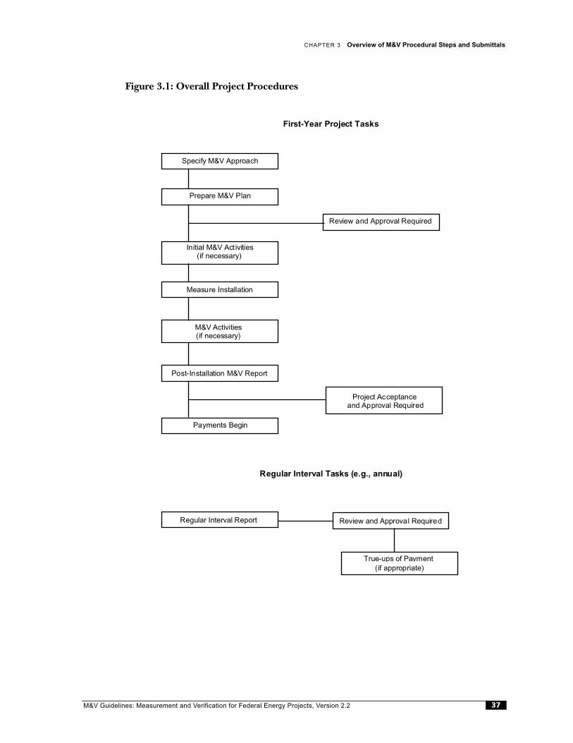
CHAPTER 3 Overview of M&V Procedural Steps and Submittals
Figure 3.1: Overall Project Procedures
Regular Interval Tasks (e.g., annual)
Regular Interval Report
True-ups of Payment(if appropriate)
Review and Approval Required
Specify M&V Approach
Prepare M&V Plan
Review and Approval Required
Initial M&V Act ivities(if necessary)
Measure Installation
M&V Activities(if necessary)
Post-Installation M&V Report
Project Acceptance and Approval Required
Payments Begin
First-Year Project Tasks
M&V Guidelines: Measurement and Verification for Federal Energy Projects, Version 2.2 37

SECTION I I Incorporating M&V into ESPCs
The roles of each party in these steps are described in the ESPC delivery order or contract, depending on the type of specific business agreements, risk allocation, and accuracy of desired verification. In general, however, the ESCO provides documenta-tion on equipment and demonstrated savings. The federal agency verifies submittals for accuracy and provides approval so the project can proceed to the next step. The submittals include the project pre-installation report, project post-installation report, and regular interval reports. As part of the review of the submittals, the federal agency conducts site inspections to confirm submittal data.
These steps should apply to most projects; however, some M&V activities (see below) might not be necessary if certain variables, used in estimating savings, are stipulated in the contract. The steps identified above are briefly described in the following paragraphs.
3.2.1 Site-Specific M&V PlanA site-specific M&V plan that is based on these M&V Guidelines must be defined. This M&V plan will consider the type of ECM or system selected, the desired level of confidence, and the level of accuracy of verification needed.
In some cases, the M&V plan requirement will be included by the agency as part of the RFP. In other cases, the ESCO will propose a site-specific plan to be finalized either before or after execution of a contract or delivery order. The decision as to whether the agency will specify the site-specific plan or the contractor will be asked to provide it could depend on the resources available to the agency preparing the RFP.
The M&V plan should include a project description, facility equipment inventories, descriptions of the proposed measures, energy and cost savings estimates, budget documentation (construction and M&V budgets), and proposed construction and M&V schedules. Details about the contents of the M&V plan are described inChapter 4.
3.2.2 Initial M&V Activities and ECM InstallationAfter the federal agency accepts the M&V plan, baseline documentation and analysis is conducted, as needed, and then project installation may proceed. Pre-installation metering is conducted in accordance with the approved, site-specific M&V plan. As soon as the federal agency accepts any required pre-installation metering andanalysis, the project can be installed. During metering and project installation, which is done by the ESCO, the federal agency may request progress reports or conduct inspections.
The major tasks associated with M&V work before the ECM installation are asfollows:
1. Pre-installation metering is conducted for a period of time required to capture all operating conditions of affected systems and/or processes. If the ESCO isresponsible for metering, the federal agency will conduct progress inspections (and/or reports), as required.
M&V Guidelines: Measurement and Verification for Federal Energy Projects, Version 2.238
CHAPTER 3 Overview of M&V Procedural Steps and Submittals
2. As specified in the M&V plan, documentation on the results of the pre-installation metering/analysis is submitted to the federal agency for theagency's review and approval.
3. The federal agency notifies the ESCO that project installation may start (or that the pre-installation M&V efforts are not complete and more effort is required by the ESCO).
4. Project installation begins.
5. The ESCO notifies the federal agency that project installation is complete.
If no pre-installation M&V activities are required, project installation approval may be given upon acceptance of the M&V plan and other non-M&V documentation.
3.2.3 Project Post-Installation Report When the measures are installed, the ESCO notifies the federal agency that the project installation is complete by submitting the project post-installation report. The report includes documentation of the project's complete installation and proper operation (e.g., commissioning) and calculations with energy and costsavings estimates. Post-installation, first-year M&V work may be conducted beforeor after submitting a project post-installation report but before submitting the first annual report.
Whether first-year M&V activities are conducted before or after submittal of the project post-installation report is defined in the M&V plan. Typically, first-year M&V activities are conducted after submittal of this report so the project installation can be approved quickly and payments to the ESCO can begin. First-year activities may be conducted before the report is submitted if they are simple and can be done quickly.
The federal agency reviews the project post-installation report, inspects the installed project, and inspects any post-installation metering as necessary. The federal agency will either (a) give its approval if the installation and documentation are acceptable or (b) decline its approval if the installation and documentation are unacceptable or issues exist that prevent a review decision. Upon the federal agency's acceptance of the project post-installation report, ESCOs may submit monthly invoices for first-year payment based on savings estimates in the accepted report.
3.2.4 Regular-Interval (Annual) ReportingRegular M&V activities are conducted periodically based on terms in the M&V plan and the contract between the federal agency and the ESCO. The ESPC program requirements (10 CFR Part 436.37) specify annual verification of savings. Therefore, in almost all cases regular interval reporting will be annual reporting, and it will be referred to as such in the rest of this document. The ESCO is encouraged, however, toprovide quarterly reports on the status of the measures and any available, updated savings reports in order to avoid surprises or delays in the approval of annual reports.
M&V Guidelines: Measurement and Verification for Federal Energy Projects, Version 2.2 39
SECTION I I Incorporating M&V into ESPCs
Annual reports contain the energy and cost savings associated with the project. If the M&V plan calls for metering, the ESCO analyzes current M&V data and submits annual reports for federal agency review and approval. These annual reportstypically include measurement-based kWh savings data. Annual report data are used for verifying levels of guaranteed savings and the basis for any required true-uppayments. These same data are also used in projecting energy savings for subsequent contract periods, and they are the basis for contract payments in the following period.
The major tasks associated with annual reports are as follows:
1. If the ESCO is responsible for any form of measurements or metering, it notifies the federal agency of the initiation of the metering and any details that require federal agency approval. Metering is then conducted continuously (or for a period of time required to capture all operating conditions of the projects)and/or affected processes. The federal agency can conduct progress inspections of metering, as required.
2. Metering data, data analysis and documentation, and inspection verificationdocumentation is presented in the annual report, or more often, asrecommended or required in the M&V plan. Federal facility personnelreview and approve the report.
3. Federal facility personnel ensure that the report and verification documentation are complete and accurate and in compliance with the contract and approved site-specific M&V plan.
As stipulated in the contract or delivery order, the federal agency may use the annual report to reconcile payments made to the ESCO for previous billing periods, since previous payments were based on estimated savings that now need to be trued-up to reflect actual savings. The estimates in the report may also be used as the basis for subsequent payments.
M&V Guidelines: Measurement and Verification for Federal Energy Projects, Version 2.240
4M&V Plan Preparation and Review
The “performance” aspect of performance contracting is affected by how energysavings are determined. The M&V plan defines project-specific M&V techniques that will be used to determine savings resulting from performance contracting projects. Therefore the M&V plan is one of the most important components of a performance contract. The ESCO typically prepares the project-specific M&V plan and submits it to the federal agency for review and approval.
This chapter provides guidance on preparing and reviewing project M&V plans.General components of an M&V plan are summarized, specific M&V issues and method considerations are explained, and an M&V review procedure is outlined.
4.1 M&V Plan Components
A site-specific M&V plan is required for each site defined in an ESPC agreement. Asingle project-specific M&V plan can be submitted for multiple sites if, and only if, each project site has the same ESCO, measures, occupancy schedule, use, and energyconsumption patterns as the others. In this instance, it is the ESCO's responsibility to document, to the satisfaction of the federal agency, that the project sites meet thesecriteria.
At a minimum, a project-specific M&V plan that uses a method described in these Guidelines must include the items listed in Table 4.1 and Table 4.2. Table 4.1 lists the itemsnecessary to describe the M&V details at the project level. Table 4.2 lists the itemsnecessary to describe the M&V details at the measure level. These items should be repeated in the M&V plan for each measure planned for the project.
It is important to realistically anticipate the costs and level of effort associated withcompleting metering and data analysis activities. Time and budget requirements are often underestimated. Improved time and budget estimates can be achieved byproperly defining the critical factors that affect energy consumption prior tocompleting the M&V plan. Understanding the project value and costs is necessary toset reasonable M&V goals and accuracy requirements.
M&V Guidelines: Measurement and Verification for Federal Energy Projects, Version 2.2 41
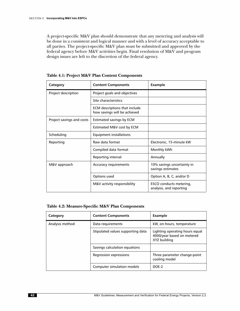
SECTION I I Incorporating M&V Into ESPCs
A project-specific M&V plan should demonstrate that any metering and analysis will be done in a consistent and logical manner and with a level of accuracy acceptable to all parties. The project-specific M&V plan must be submitted and approved by the federal agency before M&V activities begin. Final resolution of M&V and program design issues are left to the discretion of the federal agency.
Table 4.1: Project M&V Plan Content Components
Table 4.2: Measure-Specific M&V Plan Components
Category Content Components Example
Project description Project goals and objectives
Site characteristics
ECM descriptions that include how savings will be achieved
Project savings and costs Estimated savings by ECM
Estimated M&V cost by ECM
Scheduling Equipment installations
Reporting Raw data format Electronic, 15-minute kW
Compiled data format Monthly kWh
Reporting interval Annually
M&V approach Accuracy requirements 10% savings uncertainty insavings estimates
Options used Option A, B, C, and/or D
M&V activity responsibility ESCO conducts metering,analysis, and reporting
Category Content Components Example
Analysis method Data requirements kW, on-hours, temperature
Stipulated values supporting data Lighting operating hours equal 4000/year based on metered XYZ building
Savings calculation equations
Regression expressions Three parameter change-point cooling model
Computer simulation models DOE-2
M&V Guidelines: Measurement and Verification for Federal Energy Projects, Version 2.242

CHAPTER 4 M&V Plan Preparation and Review
4.1.1 Preparing Project-Specific M&V Plans Using Other MethodsIf the project-specific M&V plan is to be developed using a method that is not described in these Guidelines, the following information should be supplied by the ESCO.
• The reason why none of the M&V methods in the Guidelines are applicable.
• An overview of the method.
• A description of how baseline and post-installation inventories and equipment and system descriptions will be documented.
• A description of any spot, short-term, or long-term metering.
• A method of analysis for calculating savings.
4.2 Metering
M&V consists not only of verifying that new equipment has been installed and has the potential to save energy but also includes measuring energy consumption and energy-related variables. To determine energy savings, some measurement processes need to be conducted to identify the pre-retrofit and post-retrofit conditions. The following sections discuss metering issues that should be considered in preparing a project M&V plan.
Metering and monitor-ing
Metering protocols ASHRAE GPC 14P pump multiple point test throughout short-term monitoring
Equipment
Equipment calibration protocols NIST protocols
Metering points Flowrate, RMS power
Sampling 90% conf./10% prec.
Metering duration and interval 2 weeks/15-minute data
Baseline determination Performance factors kW/ton
Operating factors Load, on-hours
Existing service quality Zone temps, lumen level
Minimum performance standards ASHRAE 90.1 1989
Savings adjustments Party responsible for which changes
Normalized energy-use equationsConceptual approaches
Category Content Components Example
M&V Guidelines: Measurement and Verification for Federal Energy Projects, Version 2.2 43
SECTION I I Incorporating M&V Into ESPCs
In general, a project-specific M&V plan should demonstrate that metering andmonitoring will be done in a consistent, logical manner at a level of accuracyacceptable to all parties. Metering and monitoring reports must address exactly what was measured, how, with what meter, when, and by whom.
Calibration of sensors and meters to known standards (i.e., National Institute of Standards and Technology (NIST) standards) is required to ensure that datacollected are valid. Project information and metered data must be maintained in usable formats. Both “raw” and “adjusted” data should be submitted to the federal agency with post-installation and regular interval reports.
4.2.1 EquipmentFor data collection, storage, and reporting, there are three categories of metering equipment for M&V activities—each with its own advantages and disadvantages. The equipment categories include data loggers, portable loggers, and energy manage-ment systems.
Data loggers collect input typically from 3 to 30 transducers. Data loggers can collect information from a range of different inputs, conduct some analyses, prepare reports, and, typically through modems, download information for remote datacollection. They tend to be relatively expensive (when transducer and installation costs are included) and, if hard-wired, not very portable, which is an issue when only short-term measurements are required.
Portable loggers collect information about a single variable (such as light fixtureon/off status or power consumption of a motor). These tend to be inexpensive per unit, but have limited applications; downloading of data is usually done manuallyoff-site through a connection to a personal computer. Battery-powered portableloggers offer non-intrusive monitoring within an occupied space.
Energy management systems (EMS) are used for controlling systems. These would logically be an excellent option since they are often already in place and have data collection and computing capability; however, caution should be used as manysystems are not designed for data storage and reporting, and many operators arenot familiar with M&V requirements.
4.2.2 Sensor and Meter CalibrationSensors and meters used to collect M&V data should be calibrated to knownstandards (such as NIST). Forms indicating that calibration has been conducted are a required part of the M&V reports.
4.2.3 Metering and Monitoring ProtocolsTwo types of metering protocols apply to M&V. The first pertains to the M&Vprocedure and its adherence to M&V protocols (options A, B, C, and D) outlinedin this document and based on IPMVP techniques. The second pertains to
M&V Guidelines: Measurement and Verification for Federal Energy Projects, Version 2.244

CHAPTER 4 M&V Plan Preparation and Review
standardized procedures developed for measuring physical characteristics and metering specific types of equipment. ASHRAE 14P outlines standards formeasuring physical characteristics, including power, temperature, flow, pressure, and thermal energy. In addition, ASHRAE 14P lists and briefly describes standards for measuring the perfor- mance of chillers, fans, pumps, motors, boilers/furnaces, and thermal storage. The standardized equipment measurement procedures have been refined specifically for M&V methods for several equipment types. Specifically, ASHRAE 14P Annex E describes these procedures for pumps, fans, and chillers. The methods describe measurement procedures relevant to M&V options A and B.
4.2.4 Metering DurationThe duration of metering and monitoring must be sufficient to ensure an accurate representation of the amount of energy used by the affected equipment both before and after project installation. The measurements should be taken at typical system outputs within a specified (and representative) time period. These measurements can then be used to determine annual and time-of-use energy consumption. The time period of measurement must be representative of the long-term (e.g., annual) performance of the ECM or system. For example, lighting retrofits in a 24-hourwarehouse that is operated every day of the year may require only a few days of metering. A chiller retrofit, however, may require metering throughout the cooling season or perhaps for one month each season of the year.
The required length of the metering period depends on the type of ECM or system. If, for instance, the project installation is equipment that operates according to a well-defined schedule under a constant load, such as a constant-speed exhaust fan motor, the period required to determine annual savings could be quite short. In this case, short-term energy savings can be extrapolated easily to the entire year.
If the project's energy use varies across both day and season, however, as withair-conditioning equipment, a much longer metering or monitoring period may be required to characterize the system. In this case, long-term data are used todetermine annual energy savings. When the metering or monitoring is complete, the limits of the model used to characterize the system must be defined. For example, if data were taken on the chiller system only when the outside air temperature was between 50°F and 70°F, then the resulting chiller model is probably valid only within the model limits of 50°F to 70°F.
For some types of projects, metering time periods may be uncertain. For example, there is still controversy over how long lighting operating hours must be measured in office buildings to determine a representative indication of annual operating hours. In these situations, an agreement is required between the project parties todetermine the appropriate measurement period and accuracy level for the ECMsor systems under consideration.
For some projects, the metering time period can be reduced by forcing a system to go through all of its operating modes in a short period of time. For example, avariable-speed drive ventilation system that is controlled by outside air temperature may require months of data collection to capture a full range of performance data.
M&V Guidelines: Measurement and Verification for Federal Energy Projects, Version 2.2 45
SECTION I I Incorporating M&V Into ESPCs
But if the control system was over-ridden to force it to operate in various modes, the data collection may only take a day.
If energy consumption varies by more than 10% from one month to the next,sufficient measurements should be taken to document these variances. In addition, changes that will affect the base-year energy consumption adjustment by more than 10% should also be documented and explained. Any major energy consumption variances due to seasonal activity increases or periodic fluctuations must also be monitored. If these variances cannot be monitored for some reason, they must be included in the annual energy consumption figure through a mathematicaladjustment agreeable to both parties and documented in the M&V plan.
Energy use can be normalized as a function of an independent parameter such as temperature, humidity, or meals served. Once the relationship between equipment energy consumption and the parameters is established, values of independent parameters measured during the post-installation period can be used to drive the baseline model. Therefore, a project-specific M&V plan should identify criticalvariables, explain how they will be measured or documented, and discuss how they will be used in the empirical model. Additionally, assumptions and mathematicalformulas used in the M&V plan must be clearly stated.
4.2.5 SamplingSampling techniques should be used when it is unrealistic to monitor every piece of equipment affected by a retrofit. The sampling procedures outlined in Appendix D provide guidance on selecting a properly sized random sample of equipment for monitoring energy-related factors such as operating hours, RPM, or kWh. Themeasurements, taken from a sample of equipment, can then be used to estimatethe energy-related factors for the entire population.
A successful sample will be sufficiently representative of the population to enable one to draw reliable inferences about the population as a whole. The reliability with which the sample-based estimate reflects the true population is based on specified statistical criteria, such as the confidence interval and precision level, used in the sample design. The reliability of a sample-based estimate can be computed only after the metered data have been gathered. Before collecting the data, one cannot state the level of reliability that a given sample size will yield; however, one can compute the sample size that is expected to be sufficient to achieve a specified reliability level. This is done by using projections of certain values and criteria in the sample sizecalculations.
Based on the data gathered for a selected period of time, the sample size required may be reduced or increased. If the projections are too conservative, the estimate will exceed the reliability requirements. If these projections prove to be overlyoptimistic, then the reliability of the estimates will fall short of the requirements, necessitating additional data collection to achieve the specified reliability level. This method of using projections to calculate the necessary sample size is the one adopted for these guidelines.
M&V Guidelines: Measurement and Verification for Federal Energy Projects, Version 2.246
CHAPTER 4 M&V Plan Preparation and Review
4.3 Commissioning
System commissioning is the process of ensuring that as-built installed systems are functioning according to their design intent. Commissioning new or retrofit systems in buildings is one method of verifying the performance potential of an installed ECM or system. Thus, commissioning can be part of the M&V process. For complex ECMs, such as HVAC and central plant systems, commissioning is the preferred method of performance verification. Commissioning plans should be developed during the design phase after ECMs and building systems are identified.
If buildings are to realize the full potential of proposed ECMs, adequate resources must be allocated to the commissioning process. This means that time scheduled for commissioning cannot be arbitrarily reduced, and an independent commissioning authority should be appointed. This person or agency should review the designdocuments to confirm that there is sufficient information to allow the systems to be correctly commissioned and should then oversee the complete commissioningprocess described in ASHRAE Guideline 1.
In addition to performing building commissioning, the design intent and correct operation of ECMs and systems should be documented for the buildingmaintenance staff. Some ECMs such as natural ventilation, daylighting, nighttime flushing, and use of building thermal mass result in a building that behavesdifferently than a conventional building does. It is important that the commissioning contractor, building maintenance staff, and occupants understand how the building works. The federal agency may request the ESCO to conduct training sessions for the staff as part of the building commissioning to ensure that the ECMs and systems will be properly maintained and operated.
4.3.1 StandardsThese are the minimum suggested standards that should be included in thecommissioning process:
• NEBB Procedural Standards for Testing, Adjusting, Balancing of Environmental Systems; Vienna, VA: National Environmental Balancing Bureau, 1983.
• AABC National Standards 1982; Washington, DC: Associated Air BalanceCouncil, 1982.
• ASHRAE G-1 Guideline for Commissioning of HVAC Systems; Atlanta: American Society of Heating, Refrigerating and Air-Conditioning Engineers, Inc., 1989.
• ANSI/ASHRAE 111, Practices for Measurement, Testing, Adjusting andBalancing of Building Heating, Ventilation, Air-Conditioning, and Refrigerating Systems; Atlanta: American Society of Heating, Refrigerating andAir-Conditioning Engineers, Inc., 1988.
In addition to the recommendations in these standards, the commissioningauthority, as defined in ASHRAE G-1, must be independent of the installingcontractor.
M&V Guidelines: Measurement and Verification for Federal Energy Projects, Version 2.2 47
SECTION I I Incorporating M&V Into ESPCs
4.3.2 Direct Digital Controls CommissioningNearly all buildings today (aside from very small ones) have some form of directdigital controls (DDC). Although procedures for checking valve stroke andoperation, location, and calibration of sensors are well documented, there is less clarity on commissioning and verification of the software functions and sequence of operations. It is not the intention of this guideline document to define a commis-sioning procedure for DDC systems. It is vitally important, however, that the system be commissioned correctly, especially if the system will be used to verify energyperformance. True system verification requires each point and sequence ofoperation be checked. For a large and complex building, this may involve twocontrols engineers for approximately four weeks.
4.3.3 Documenting the ProcessDocumentation of the commissioning process is critical in performance contracting. Clear documentation of all set points and air and water quantities, as well as anydeviations from the design documents are an essential part of the post-installation verification process. Both the commissioning agent and the performanceverification agent must review the proposed documentation before commissioning starts. This should ensure that the level of information presented in completeddocuments is adequate for the performance verification method selected.
4.3.4 Using Energy Management Systems or Data LoggersUsed to collect and analyze data, benefits, and hazards, the building energymanagement system can provide much of the monitoring necessary for theverification process. The system and software requirements must be specified sothat the building EMS can be a useful tool for verification as well as for controlling building systems.
Some parameters may need monitoring for verification, but they might not be required for control. These points must be specified in the design documents.Electric power metering is an example. Trending of small power, lighting, and main feed power consumption may be very useful for high-quality verification. Otherfunctions that can easily be incorporated into the software are automatic recording of changes in set-points. The evaluation team can have a direct read-only connection into the EMS via a modem link. This allows all the trending data to be analyzed and collated by the evaluation team in their office. It is not unusual for many of the trending capabilities required for verification to be incorporated in an EMS;however, often the building facility staff is not properly trained in the use of thesystem and is unaware of the many additional monitoring and diagnostic capabilities of the system.
4.4 Inspections
Pre-installation, post-installation, and regular interval inspections (e.g., annual) by federal agency representatives may be conducted to confirm the documentation
M&V Guidelines: Measurement and Verification for Federal Energy Projects, Version 2.248
CHAPTER 4 M&V Plan Preparation and Review
submitted to the federal agency by the ESCO. These inspections, or confirmationvisits, by agency representatives are very important. If the federal agency believes that the conditions at the site are not accurately represented by the ESCO's submittals, the ESCO will be allowed to address the problem and make a new submittal. If the ESCO and federal agency cannot agree on site conditions, however, a contract or project may be modified or terminated. The federal agency's inspection personnel do not have the authority to approve changes to contract documents or ESCOsubmittals to the federal agency. The federal agency's authorized representative(typically, an agency contracting officer) must approve any changes.
4.5 Baseline Characterization
It is not possible to measure the absence of energy use directly. Instead, energysavings must be determined from comparing energy use before and after a retrofit. Therefore, pre-retrofit or baseline characterization is as important as post-installation measurements. The baseline characterization consists of identifying the performance and operating factors that influence energy consumption as well as determining their values through measurements.
A complete baseline characterization is necessary because simple comparison bysubtraction of post-installation energy use from baseline energy use is insufficient for accurately estimating savings. A simple comparison does not account for extraneous factors, such as weather and occupancy, that influence energy consumption. Proper assessment commonly involves projecting post-retrofit conditions onto the baseline period. The issues surrounding baseline adjustments are described in Section 4.5.1 below. Additional considerations in defining baseline performance and servicequality are presented in Sections 4.5.2 and 4.5.3.
4.5.1 Baseline AdjustmentsBaseline adjustments required during the performance period of a contract are a common area of contention in performance contracts. Thus, even if utility billanalysis is used to determine energy savings, a complete and detailed audit (e.g., a detailed energy survey) is required. Examples of situations in which the baseline must be adjusted are changes in the amount of space being air-conditioned, changes in auxiliary systems (towers, pumps, etc.), and changes in occupancy or schedule.
If the baseline conditions for these factors are not well documented, it becomesdifficult, if not impossible, to properly adjust them when they change and require changes to payment calculations. For example, if a chiller retrofit takes place in a building with 100,000 square feet of conditioned space, and later (during theperformance period) the building's conditioned space is reduced to 75,000 square feet, post-installation energy use would be less and calculated savings would be higher, perhaps inappropriately higher. If there were no records of how much space was originally conditioned, however, the baseline could not be adjusted to properly reflect the amount of “true” savings and how much the ESCO should be paid.
M&V Guidelines: Measurement and Verification for Federal Energy Projects, Version 2.2 49
SECTION I I Incorporating M&V Into ESPCs
Information about baseline energy consumption that an ESCO submits in the pre-installation report is an estimate. This estimate is determined through energy audits and site surveys. It is common, however, for this estimated baseline to change after actual metering data has been collected during pre-installation M&V activities, or if operating conditions change significantly after project installation. This change is called baseline adjustment. ESCOs must submit, as part of the M&V plan, a description of how they will adjust the baseline if metering data and/or post-installationoperating conditions are different from those used to determine the estimatedbaseline. The following are examples of why and how baselines are adjusted:
• Changes in weather or occupancy data. Such changes are expected andpredictable, so the M&V plan should include procedures for dealing with such changes. These procedures might include (1) recalculating baselineconsumption rates using performance-period weather or occupancy data, (2) recalculating performance-period consumption rates using baseline weather or occupancy data, or (3) stipulating typical weather or occupancy conditions.
• Changes in hours of operation or tenant improvements. These changes may be predictable, but because of the numerous unknowns and possible “what-if”scenarios they involve, ESCOs do not need to provide detailed calculationmethods covering each eventuality. Therefore, a more conceptual approach is appropriate. In general, an ESCO is responsible for delivering savings that would not have otherwise occurred without the ESCO's intervention. Therefore, decreases in a facility's operating hours or reductions in the amount of condi-tioned space will not be counted towards savings. In addition, retrofits or tenant improvements installed by a federal agency that are not part of the projectcannot be counted toward savings. If, however, increases in operating hours are one of the benefits of the ESCO's project (e.g., lighting retrofit), these can be counted in the savings calculation if agreed to by the federal agency. ESCOs can indicate in their M&V plan (a) which party is responsible for decreases or increases in energy savings associated with different categories of changes,(b) whether or not an ESCO can claim credit for savings associated with differentcategories of change, or (c) which categories of change are eligible for baseline adjustments.
• Changes in the actual function of a facility, such as a warehouse changing into office space. Such unpredictable changes are addressed in the termination, default, and arbitration clauses contained in the ESPC. Reductions in energyconsumption caused by building vacancies, decreased production, and otherfundamental operational changes are not considered the basis for savings.
• With Option A, baseline adjustments are less likely to be required since many of the operating or performance factors are stipulated, such as cooling load. This is one reason why Option A can be less accurate but easier and less expensive to implement.
• Option B involves metering techniques. Baseline capacity data are not changed (e.g., lighting wattages, chiller kW/ton, motor kW), but baseline “operatingvalues” can be changed by the use of post-installation monitoring data(e.g., operating hours and ton-hours).
M&V Guidelines: Measurement and Verification for Federal Energy Projects, Version 2.250
CHAPTER 4 M&V Plan Preparation and Review
• For Option C, billing analysis, typical values or post-installation values are defined for baseline and post-installation independent variables that influence energy use (e.g., weather and occupancy). It is important to agree in advance on thevariables to be used.
• For Option D, calibrated simulation, it is important to agree in advance on how the model will be calibrated and what changes will require a new simulation run. For most retrofit and new construction projects, baseline and post-installation models are calibrated and then run with typical data (e.g., weather data).Thereafter, they are not modified unless major changes occur in the building. Annual verifications are expected, but normally the models do not need to be run again.
4.5.2 Minimum Energy StandardsWhen laws or federal agency standard practice require a certain level of efficiency, savings may be based on the difference between the energy usage of the newequipment and baseline equipment that meets the legal or standard practice requirements. In these situations, the baseline energy and demand consumption must be equal to or less than any applicable minimum energy standards. If this requirement exists, it will be specified in the federal agency's RFP and/orgovernment-defined baseline.
4.5.3 Maintaining Service QualityThe measures installed under ESPC programs should maintain or improve thequality of service provided to the federal agency by the affected equipment orsystems. For example, lighting projects that reduce lighting levels must maintain some minimum standards (i.e., the minimum Illuminating Engineering Society (IES) standard for the space's primary use.)
In this document, however, verifying the performance standards is not addressed. Specific facility performance requirements are defined in the RFPs for ESCOservices.
4.6 Interactive Effects
It is commonly understood that ECMs and energy systems interact with each other. Reduced lighting loads, for example, can reduce air-conditioning energyconsumption but increase heating consumption. Detailed relationships between many dissimilar but interactive ECMs are not known, however, and the methods formeasuring interactive effects are not cost-effective for many applications.
For lighting projects, one of the following three approaches can be taken to account for savings associated with interactive effects:
M&V Guidelines: Measurement and Verification for Federal Energy Projects, Version 2.2 51
SECTION I I Incorporating M&V Into ESPCs
1. Ignore interactive effects.
2. Use mutually agreed-upon default values that are applicable based on thesite-specifics associated with building type and HVAC equipment type. The default values can either be assigned on the basis of available information fortypical buildings or developed on the basis of computer model simulations for typical building conditions. A critical element of this approach is for the ESCO or federal agency to demonstrate in the baseline lighting survey that the measures or systems are in air-conditioned space. If the space is also heated, the post-installation energy consumption needs to be adjusted upward to account for the increase in the heating load caused by losses in internal heat gains from efficient lighting equipment.
3. Propose a method to measure and estimate interactive effects. The federal agency and/or ESCO will need to agree on the merit and reasonableness of the proposed approach which may include either (a) directly measuring the effects, (b) simulating the HVAC (heating and cooling) interactive effects using a fully documented computer program, or (c) using a utility meter billing analysis approach that captures interactive effects in the total predicted savings. All these methods must be proposed and reviewed on a site-specific basis.
4.7 Calculating Energy Costs
The goal of ESPC is to reduce energy, water, and/or operations and maintenance costs at federal facilities. The M&V plan should be designed to provide energy, water, or operating savings information in such a way that cost savings can be estimated.
For example, energy cost savings will be determined using calculated energy savings and the appropriate cost per unit of energy saved. In most cases the unit cost of energy will be based on a servicing utility's energy rate schedules at the time the project is implemented. The unit cost of energy that will be used in calculating energy cost savings must be defined in sufficient detail in the contract to allow sav-ings to be calculated using each of the factors that affect cost savings. These factors include items such as (for electric bills) kWh saved, kW saved, power factor, kW ratchets, and energy rate tiers.
For performance contracts with cost savings based on peak or billing period load reductions, an M&V method should be selected that provides energy savings data by time-of-use periods corresponding to the facilities' rate structure. For example, at a federal prison, the water heating peak load over a two-minute averaging period might be 252 kW, 228 kW over 15 minutes, or 192 kW using 60-minute time periods of analysis. Considerable error in cost savings estimates are introduced by data that do not correspond to the rate structure (15 minutes, in this case). Thus, it is critical that M&V plans reflect the effects of time-of-use and block rate schedules.
M&V Guidelines: Measurement and Verification for Federal Energy Projects, Version 2.252
CHAPTER 4 M&V Plan Preparation and Review
4.8 Reporting
4.8.1 Standardized FormsSample survey forms for lighting and motors projects are presented in Appendix C. These forms, which are subject to change, may be required by the sponsoring federal agencies. The forms are based on a particular seasonal and time-of-use utility rate structure. Other rate structures will require different reporting formats for operating hours. Equipment surveys submitted by ESCOs are expected to be comprehensive, accurate (for example, ±5%), and current (completed within a reasonable time before submittal).
Data and surveys submitted should be provided in both electronic and hard-copyformats as specified by the federal agency.
4.8.2 Submitting Metered DataWhen submitting an M&V report, ESCOs should provide the data they collect during M&V activities in the formats specified in the M&V plan. Metered data must beprovided in formats that are usable by the federal agency and based on products or software that are publicly available. If special software products are required for the reading or analysis of ESCO submittals, the federal agency may reject the data or request that the ESCO provide the software.
Both “raw” and “compiled” data must be submitted to the federal agency in support of surveys, savings estimates, and calculations. For billing analysis and computersimulation M&V methods, electronic and hard copy input and output files must be provided. Compiled survey data must be submitted in both hard-copy and electronic formats using either Lotus 123© or Microsoft Excel©, as specified by the Federal agency.
4.8.3 Communicating M&V Activities to Federal AgenciesESCOs must notify the federal agency whenever they are about to (a) install andcalibrate metering equipment and/or (b) remove metering equipment. Enough lead-time must be given in case the federal agency decides to conduct a siteinspection before the equipment is either installed or removed.
Verbal communication concerning changes or acceptance of ESCO M&V submittals is not binding on the federal agency. All submittals, changes to submittals, and approvals must be in writing and signed by an authorized party, as indicated in the ESPC.
M&V Guidelines: Measurement and Verification for Federal Energy Projects, Version 2.2 53
SECTION I I Incorporating M&V Into ESPCs
4.9 Third-Party Reviewers
Often the ESCO has more expertise and experience than the federal agency indealing with performance contracts and ECM savings. Therefore, it is often cost-effective and beneficial for an agency to engage third-party M&V professionals to assist in defining or reviewing ESCO-prepared M&V plans and analyzing the results. This helps provide a “level playing field” for negotiation and determination ofsavings and payments to the ESCO. M&V professionals are typically engineers with experience and knowledge in verifying ECM savings, ECM technologies, andperformance contracting. FEMP can help by providing these services or making referrals.
4.10 M&V Plan Review
As noted previously, the level of savings uncertainty and thus effort required to verify both a project's potential to perform and its actual performance will vary from project to project. The project-specific M&V plan should be prepared with theseconsiderations in mind. Section 2.4.2 of the Guidelines discusses some factors that affect the decision of which M&V option, method, and technique to use for each ESPC project. The section below provides a framework for applying theseconsiderations in reviewing the appropriateness of an M&V plan proposed for afederal facility.
4.10.1 Assessment ProcedureA proper M&V assessment includes evaluating the following aspects of the M&V plan to determine if it is reasonable for the specified project:
• Examine ECMs, prioritize by savings amount, and assess error tolerances.
• Review M&V approach for each ECM. Expect diversity in strategies between ECMs.
• Look for documented M&V assumptions and stipulations. Evaluate forappropriateness based on supporting data.
• Assess M&V cost break-down by ECM to determine if level of effort is justified.
Examine ECMsTo facilitate assessing the M&V rigor justified for each measure, it is helpful to rank the measures according to the cost savings anticipated for each. In addition, the uncertainty of the savings associated with each measure should be noted. Onesimplistic measure of uncertainty is the complexity of the measure. The measure complexity “ranking” can correspond to the measure categories listed in Section 2.5.2 that are ordered by increasing variability of load and operating patterns. A lower position in the list corresponds to a more complex measure. More rigorous (and expensive) M&V approaches are appropriate for high cost savings measures that are complex. Less rigorous M&V approaches are appropriate for less complex measures. In general, the M&V procedures associated with high savings measures should be more closely scrutinized than the low savings measures.
M&V Guidelines: Measurement and Verification for Federal Energy Projects, Version 2.254
CHAPTER 4 M&V Plan Preparation and Review
Review M&V ApproachesFor projects comprising a variety of conservation measures, one should expectdiversity between the M&V approaches proposed for each measure. Of course if all measures have low complexity (i.e., constant load, constant operation), an Option A approach may be justified for each. Otherwise, a variety of options can be expected. In reviewing the M&V approaches, the following questions should be asked:
• Is the rigor (or lack of rigor) associated with the M&V approaches warranted?
• Do M&V methods match the measure savings/complexity priorities?
• Is the model calibration occurring at the desired level (option D)?
Evaluate Assumptions/StipulationsThe engineering assumptions and stipulations that affect energy consumption and savings calculations must be documented in the M&V plan. In addition, thepresented values should be supported by data obtained from the manufacturer,similar projects, or measurements. As part of the assessment, the following questions should be asked:
• Are operating hours reasonable? Do they correspond to the project building activities?
• Is the stipulated value subject to sizeable variation?
• Are measurements being made over the full range of operating conditions/loads?
• Do projected savings and baseline values correspond to current utility bill data?
Assess M&V CostsIt is important to couple the measure M&V cost with the estimated cost savings to assess if the level of M&V effort is justified by the level of savings. Therefore, the M&V plan should include a break-out of costs by measure. In assessing the M&V costs, the following should be considered:
• Is the cost of the M&V approach consistent with the projected ECM savings (i.e., both high or both low)?
• Are M&V costs consistent with the level of effort?
• Do the majority of the M&V costs occur up front? If so, are they consistent with the level of effort required up-front?
M&V Guidelines: Measurement and Verification for Federal Energy Projects, Version 2.2 55
5M&V Quick-Start Guidelines
This chapter summarizes materials presented in previous chapters to providequick-start M&V guidelines. The reader will find the chapter most useful after becoming familiar with the general M&V concepts and procedures presented in Chapters 1–4. The chapter guidelines can be used as a quick reference for checking project-specific M&V plan contents and assessing the appropriateness of theproposed M&V approaches. The figures and tables included in the chapter are listed below. For each, a brief description of its application is provided, as well as thesection that contains more detailed information on the topic.
Figure 5.1 Overall Project ProceduresThe flowchart graphically depicts the steps involved in the M&V process and the activities usually assumed by the ESCO and the federal agency (ESCO activities on left, agency activities on right). This figure is described in detail in section 3.2.
Table 5.1 Overview of M&V OptionsThis table provides a quick summary of the characteristics of M&V Options A, B, C, and D. More information about the options can be found in section 2.3 as well as Section III (Option A), Section IV (Option B], Section V (Option C), and Section VI (Option D).
Table 5.2 Ranking ECM Complexity This table ranks ECM complexity according to performance and operatingcharacteristics (i.e., constant or variable). Higher ECM complexity may justify more rigorous and costly M&V procedures especially if the associated savings are high yet uncertain. Section 2.5 describes selecting M&V methods and rigor in detail.
Table 5.3 M&V Components Affecting Level of Effort and CostsThis table presents considerations that affect the level of effort and cost required to complete the project M&V. The summary is useful for assessing if the estimated M&V cost is justified from the level of effort described. Section 2.4 and Chapter 4 describe such M&V considerations in more detail.
Figure 5.2 M&V Content Requirement Checklist for M&V Approach(Initial Proposal)This checklist outlines the M&V plan contents that should be included in the initial proposal submitted by the ESCO. The initial proposal may also be referred to as the pre-installation report. More information about M&V plan content requirements are described in Section 2.2 and in Chapter 4.
M&V Guidelines: Measurement and Verification for Federal Energy Projects, Version 2.256

CHAPTER 5 M&V Quick-Start Guidelines
Figure 5.3 Content Requirement Checklist for M&V Plan and PeriodicSubmittals (Final Proposal)Similar to the initial proposal checklist, this checklist outlines the M&V plancontents that should be included in the final proposal or periodic submittalsprovided by the ESCO. More information about M&V plan content requirementsare described in Section 2.2 and in Chapter 4.
Figure 5.4 Guidelines for M&V Plan ReviewThis checklist outlines issues to be considered in assessing the appropriateness ofthe proposed M&V plan. The Guidelines also address these issues in Sections 2.5and 4.10.
M&V Guidelines: Measurement and Verification for Federal Energy Projects, Version 2.2 57
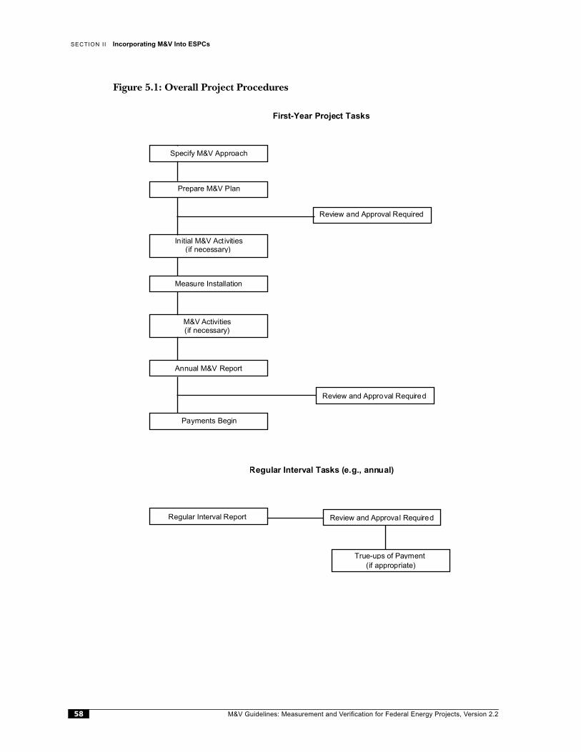
SECTION I I Incorporating M&V Into ESPCs
Figure 5.1: Overall Project Procedures
Regular Interval Tasks (e.g., annual)
Regular Interval Report
True-ups of Payment(if appropriate)
Review and Approval Required
Specify M&V Approach
Prepare M&V Plan
Review and Approval Required
Initial M&V Act ivities(if necessary)
Measure Installation
M&V Activities(if necessary)
Annual M&V Report
Review and Approval Required
Payments Begin
First-Year Project Tasks
M&V Guidelines: Measurement and Verification for Federal Energy Projects, Version 2.258
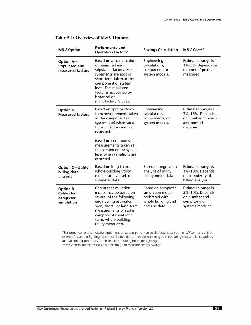
CHAPTER 5 M&V Quick-Start Guidelines
Table 5.1: Overview of M&V Options
*Performance factors indicate equipment or system performance characteristics such as kW/ton for a chiller or watts/fixture for lighting; operation factors indicate equipment or system operating characteristics such as annual cooling ton-hours for chillers or operating hours for lighting.**M&V costs are expressed as a percentage of measure energy savings.
M&V OptionPerformance and Operation Factors*
Savings Calculation M&V Cost**
Option A—Stipulated and measured factors
Based on a combination of measured andstipulated factors. Mea-surements are spot or short term taken at the component or system level. The stipulatedfactor is supported by historical ormanufacturer’s data.
Engineeringcalculations,component, orsystem models.
Estimated range is 1%–3%. Depends on number of points measured.
Option B—Measured factors
Based on spot or short-term measurements taken at the component orsystem level when varia-tions in factors are not expected.
Based on continuous measurements taken at the component or system level when variations are expected.
Engineeringcalculations,components, orsystem models.
Estimated range is 3%–15%. Depends on number of points and term ofmetering.
Option C—Utility billing data analysis
Based on long-term, whole-building utility meter, facility level, or submeter data.
Based on regression analysis of utilitybilling meter data.
Estimated range is 1%–10%. Depends on complexity of billing analysis.
Option D—Calibrated computer simulation
Computer simulation inputs may be based on several of the following: engineering estimates; spot, short-, or long-term measurements of system components; and long-term, whole-buildingutility meter data.
Based on computer simulation model calibrated with whole-building and end-use data.
Estimated range is 3%–10%. Depends on number and complexity ofsystems modeled.
M&V Guidelines: Measurement and Verification for Federal Energy Projects, Version 2.2 59
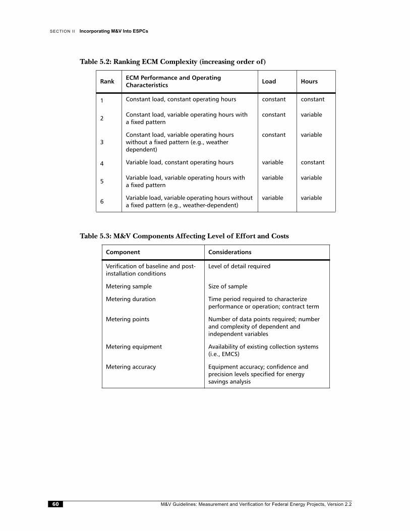
SECTION I I Incorporating M&V Into ESPCs
Table 5.2: Ranking ECM Complexity (increasing order of)
Table 5.3: M&V Components Affecting Level of Effort and Costs
RankECM Performance and Operating Characteristics
Load Hours
1 Constant load, constant operating hours constant constant
2Constant load, variable operating hours witha fixed pattern
constant variable
3Constant load, variable operating hourswithout a fixed pattern (e.g., weatherdependent)
constant variable
4 Variable load, constant operating hours variable constant
5Variable load, variable operating hours witha fixed pattern
variable variable
6Variable load, variable operating hours without a fixed pattern (e.g., weather-dependent)
variable variable
Component Considerations
Verification of baseline and post-installation conditions
Level of detail required
Metering sample Size of sample
Metering duration Time period required to characterizeperformance or operation; contract term
Metering points Number of data points required; number and complexity of dependent andindependent variables
Metering equipment Availability of existing collection systems (i.e., EMCS)
Metering accuracy Equipment accuracy; confidence andprecision levels specified for energysavings analysis
M&V Guidelines: Measurement and Verification for Federal Energy Projects, Version 2.260
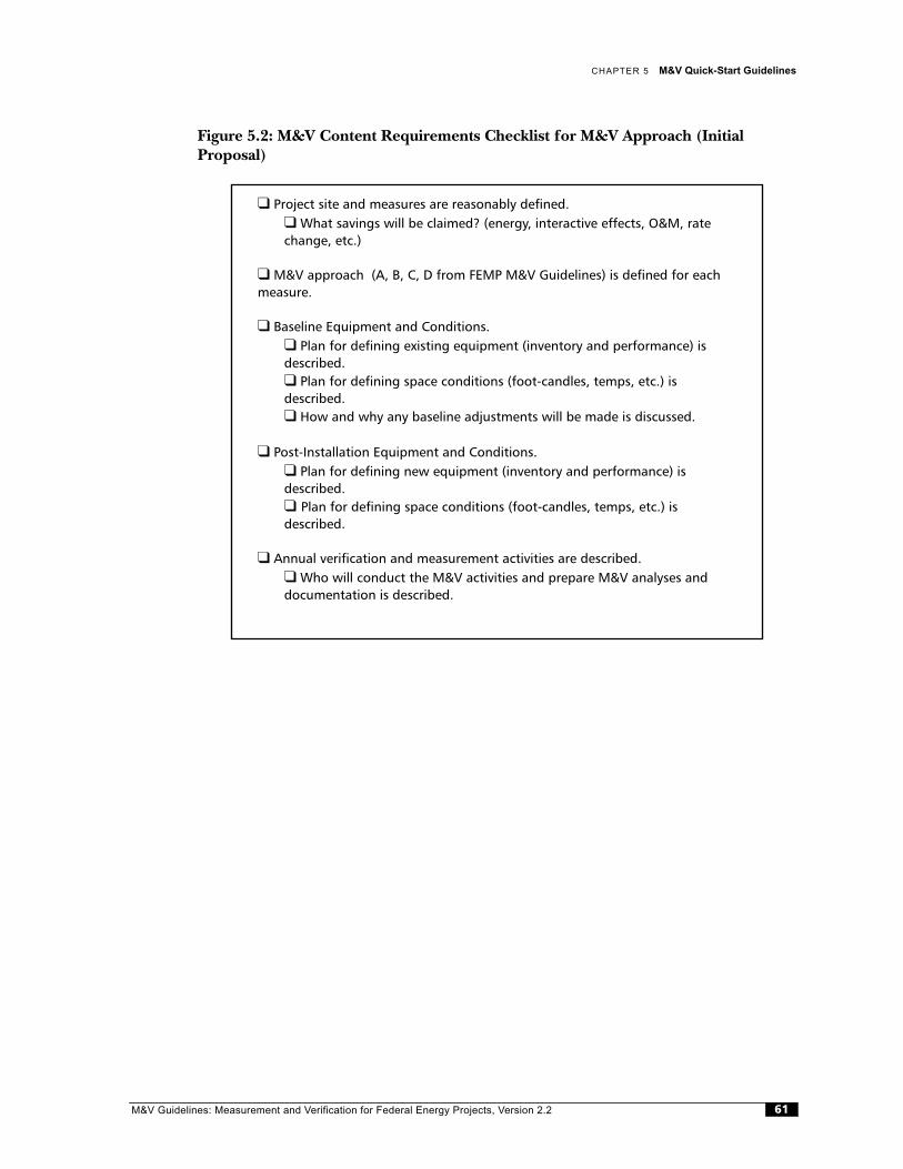
CHAPTER 5 M&V Quick-Start Guidelines
Figure 5.2: M&V Content Requirements Checklist for M&V Approach (Initial Proposal)
❑ Project site and measures are reasonably defined.❑ What savings will be claimed? (energy, interactive effects, O&M, rate change, etc.)
❑ M&V approach (A, B, C, D from FEMP M&V Guidelines) is defined for each measure.
❑ Baseline Equipment and Conditions.❑ Plan for defining existing equipment (inventory and performance) is described.❑ Plan for defining space conditions (foot-candles, temps, etc.) is described.❑ How and why any baseline adjustments will be made is discussed.
❑ Post-Installation Equipment and Conditions.❑ Plan for defining new equipment (inventory and performance) is described.❑ Plan for defining space conditions (foot-candles, temps, etc.) is described.
❑ Annual verification and measurement activities are described.❑ Who will conduct the M&V activities and prepare M&V analyses anddocumentation is described.
M&V Guidelines: Measurement and Verification for Federal Energy Projects, Version 2.2 61

SECTION I I Incorporating M&V Into ESPCs
Figure 5.3: Content Requirement Checklist for M&V Plan and Periodic Submittals (Final Proposal)
❑ Project site and measures are defined.❑ What savings will be claimed? (energy, interactive effects, O&M, rate change, etc.)❑ How will these ancillary savings be treated?
❑ M&V method(s) (chapters), from FEMP M&V Guidelines, is defined.
❑ Details of how calculations will be made are defined. All equations are shown. ❑ Provided information shows how collected data and assumptions are used.❑ Energy pricing information and assumptions are defined. (fixed cost, inflated per EIA...)
❑ Baseline Equipment and Conditions.❑ Existing equipment (inventory and performance) is defined.❑ Space conditions (foot-candles, temps, etc.) are defined. ❑ Assumptions and stipulations—show supporting information ormeasurements.❑ How and why any baseline adjustments will be made is discussed.
❑ Post-Installation Equipment and Conditions.❑ Plan for defining new equipment (inventory and performance) is described.❑ Plan for defining new space conditions (foot-candles, temps, etc.) is described.❑ Assumptions and stipulations—show supporting information ormeasurements to be taken.
❑ Metering equipment is specified.❑ Schedule of metering, including duration and when it will occur, is defined.❑ Who will provide equipment, establish and ensure its accuracy, and perform calibration procedures is described.❑ How data from metering will be validated and reported, including formats, are defined.❑ How electronic, formatted data, directly from a meter or data logger, will be provided.❑ Any sampling that will be used, sample sizes, and documentation on how sample sizes were selected, are defined.
❑ Annual verification and measurement activities are defined.❑ Who will conduct the M&V activities and prepare M&V analyses anddocumentation is defined.❑ How quality assurance will be maintained and repeatability confirmed is defined.❑ Reports are defined, including what they will contain and when they will be provided. ❑ Electronic formats and software programs to be used for reporting are defined.
❑ Initial and annual M&V costs for each measure (totals only).
M&V Guidelines: Measurement and Verification for Federal Energy Projects, Version 2.262

CHAPTER 5 M&V Quick-Start Guidelines
Figure 5.4: Guidelines for M&V Plan Review
❑ Examine ECMs.❑ Rank cost savings from measures❑ Assess measure complexity❑ Assess savings error tolerance
❑ Expect diversity of M&V strategies❑ Stipulations and engineering estimates❑ Spot/short-term measurements❑ Continuous measurements❑ Modeling
❑ Assess assumptions and stipulations❑ Are operating hours reasonable? Do they match the facility's activities?❑ Is stipulated value subject to wide variations?❑ Are measurements being made over the full range of loads?
❑ Evaluate M&V costs❑ Is each ECM M&V cost appropriate for the projected level of savings?❑ Is the cost of the M&V appropriate for the level of effort required?❑ Do the majority of M&V costs occur up front? If so, are they in accordance with the level of effort required?
M&V Guidelines: Measurement and Verification for Federal Energy Projects, Version 2.2 63

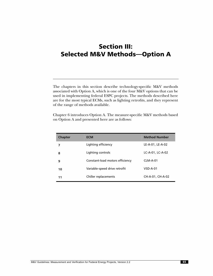
M&V Guidelines:
Section III:Selected M&V Methods—Option A
The chapters in this section describe technology-specific M&V methodsassociated with Option A, which is one of the four M&V options that can beused in implementing federal ESPC projects. The methods described hereare for the most typical ECMs, such as lighting retrofits, and they representof the range of methods available.
Chapter 6 introduces Option A. The measure-specific M&V methods basedon Option A and presented here are as follows:
Chapter ECM Method Number
7 Lighting efficiency LE-A-01, LE-A-02
8 Lighting controls LC-A-01, LC-A-02
9 Constant-load motors efficiency CLM-A-01
10 Variable-speed drive retrofit VSD-A-01
11 Chiller replacements CH-A-01, CH-A-02
Measurement and Verification for Federal Energy Projects, Version 2.2 65
6Introduction to Option A
An Option A-based M&V method involves a retrofit or system-level M&V assessment. The approach is intended for retrofits where either performance factors (e.g., end-use capacity, demand, power) or operational factors (lighting operational hours, cooling ton-hours) can be spot or short-term measured during the baseline and post-installation periods. The factor not measured is stipulated based on assumptions, analysis of historical data, or manufacturer's data. Using a stipulated factor isappropriate only if supporting data demonstrates its value is not subject tofluctuation over the term of the contract.
All end-use technologies can be verified using Option A; however, the accuracy of this option is generally inversely proportional to the complexity of the measure. In addition, within Option A, various methods and levels of accuracy in verifyingperformance/operation are available. The level of accuracy depends on the validity of assumptions, quality of the equipment inventory, and whether spot/short-term measurements are made. The penalty associated with low accuracy is not achieving the estimated measure savings and the associated utility bill cost reductions.
Option A can be applied when identifying the potential to generate savings is the most critical M&V issue, including situations in which:
• The magnitude of savings is low for the entire project or a portion of the project to which Option A can be applied.
• The risk of achieving savings is low or ESCO payments are not directly tied to actual savings.
6.1. Approach
Option A is an approach designed for projects in which the potential to generatesavings must be verified, but the actual savings can be determined from stipulated factors, short-term data collection, and engineering calculations. Post-installation energy use is not measured throughout the term of the contract. Post-installation and perhaps baseline energy use is predicted using an engineering or statisticalanalysis of information that does not involve long-term measurements.
M&V Guidelines: Measurement and Verification for Federal Energy Projects, Version 2.266

CHAPTER 6 Introduction to Option A
With Option A, savings are determined by measuring the capacity, efficiency, oroperation of a system before and after a retrofit and by multiplying the difference by a stipulated factor. Stipulation is the easiest and least expensive method of etermining savings. It can also be the least accurate and is typically the method with the greatest uncertainty of savings. This level of verification may suffice for certain types of projects in which a single factor represents a significant portion of thesavings uncertainty. Option A is appropriate for projects in which both parties agree to a payment stream that is not subject to fluctuation due to changes in theoperation or performance of the equipment. Payments could be subject to change based on periodic measurements, however.
6.2. M&V Considerations
Option A includes procedures for verifying the following:
• Baseline conditions have been properly defined.
• The equipment and/or systems contracted to be installed were installed.
• The installed equipment/systems meet contract specifications in terms ofquantity, quality, and rating.
• The installed equipment is operating and performing in accordance withcontract specifications and is meeting all functional tests.
• The installed equipment/systems continue, during the term of the contract, to meet contract specifications in terms of quantity, quality, rating, operation, and functional performance.
This level of verification is all that is contractually required for certain types ofperformance contracts. Baseline and post-installation conditions (e.g., equipment quantities and ratings such as lamp wattages, chiller kW/ton, or motor kW)represent a significant portion of the uncertainty associated with many projects.
All end-use technologies can be verified using Option A; however, the accuracy of this option is generally inversely proportional to the complexity of the measure. Thus, the savings from a simple lighting retrofit will typically be more accurately estimated with Option A than the savings from a chiller retrofit. If greater accuracy is required, Options B, C, or D may be more appropriate.
Within Option A, various methods and levels of accuracy in verifying performance are available. The level of accuracy depends on the quality of assumptions made, and it can also depend on whether an inventory method is used for ensuring nameplate data and quantity of installed equipment or whether short-term measurements are used for verifying equipment ratings, capacity, operating hours and/or efficiency. The potential to generate savings may be verified through observation, inspections, and/or spot/short-term metering conducted immediately before and/or immedi-ately after installation. Annual (or some other regular interval) inspections may also be conducted to verify an ECM's or system's continued potential to generate savings.
M&V Guidelines: Measurement and Verification for Federal Energy Projects, Version 2.2 67

SECTION I I I Selected M&V Methods Option A
Savings potential can be quantified using any number of methods, depending on contract accuracy requirements. Equipment performance can be obtained either directly (through actual measurement) or indirectly (through the use ofmanufacturer data). There may be sizable differences between publishedinformation and actual operating data. Where discrepancies exist or are believed to exist, field-operating data should be obtained. This could include spot measurement for a constant load application. Short-term M&V can be used if the application is not proven to be a constant load. Baseline and post-installation equipment should be verified with the same level of detail. Either formally or informally, all equipment baselines should be verified for accuracy and for concurrence with stated operating conditions. Actual field audits are almost always required.
M&V Guidelines: Measurement and Verification for Federal Energy Projects, Version 2.268
7
Methods:
LE-A-01
LE-A-02
Lighting Efficiency: No Metering and Metering of Fixture Wattages Only
7.1 ECM Definition
Lighting ECM projects covered by this verification plan are as follows:
• Retrofits of existing fixtures, lamps, and/or ballasts with an identical number of more energy-efficient fixtures, lamps, and/or ballasts
• De-lamping with or without the use of reflectors
These lighting efficiency projects reduce demand; however, the fixtures are assumed to have the same pre- and post-retrofit operating hours.
7.2 Overview of Verification Methods
Two verification methods are covered in this chapter. For both methods, the hours of operation are stipulated. The methods differ in how the fixture wattages aredetermined.
Surveys are required of existing (baseline) and new (post-installation) fixtures.Corrections may be required for non-operating fixtures. Light level requirements may be specified for projects that involve reducing lighting levels.
Method LE-A-01 does not require metering of fixtures. Fixture wattages will be from a standard table unless other documentation, such as the manufacturer's data, is provided.
Method LE-A-02 requires spot or short-term wattage measurements of a representative sample of baseline and post-installation fixtures or fixture circuits to establish demand. This method is more time-consuming and expensive, but it may result in more accurate savings estimates if fixture wattage measurements are done carefully.
M&V Guidelines: Measurement and Verification for Federal Energy Projects, Version 2.2 69
SECTION I I I Selected M&V Methods Option A
7.3 Calculation of Demand and Energy Savings
7.3.1 Baseline DemandThe baseline conditions identified in the pre-installation equipment survey may be defined by either the federal agency or the ESCO. If the baseline is defined by the federal agency, the ESCO will have an opportunity to verify the baseline. If thebaseline is defined by the ESCO, the federal agency will verify the baseline.
In the pre-installation equipment survey, the equipment to be changed and the replacement equipment to be installed are inventoried. The location of theequipment (e.g., the rooms it is in) and building floor plans should be included with the survey submittal. The surveys will include, in a set format, fixture, lamp andballast types, usage area designations, counts of operating and non-operatingfixtures, and whether the room is air-conditioned and/or heated.
Method LE-A-01—No MeteringFixture wattages will be from a standard table unless other documentation isprovided. A standard table of fixture wattages should contain common lamp andballast combinations. If a fixture is not found in the table, the party conducting the pre-installation equipment survey should either (a) conduct instantaneous wattage measurements for a representative sample of fixtures or (b) provide an approved, documented source of the fixture wattages for approval by the other party.
In general, a standard table of fixture wattages should be used for the baselinefixtures, and documented manufacturers' data should be used for post-installation fixtures.
Method LE-A-02—Fixture Wattage Metering Fixture wattages will be measured. An example of a metering protocol is:
The ESCO will take 15-minute, true root-mean-square (RMS) wattage measurements from at least six fixtures representative of the baseline and post-installation fixtures (actual values may vary by application). Readings will be averaged to determine per-fixture wattage values. For post-installation fixtures, readings should be taken only after the new fixtures have been operating for at least 100 hours. Meters used for this task will be calibrated and have an accuracy of ±2% of reading or better.
7.3.2 Adjustments to Baseline DemandBefore the new lighting fixtures are installed, adjustments to the baseline demand may be required for non-operating fixtures. In addition, after ECM installation, adjustments to baseline demand may be required because of remodeling or changes in occupancy. Methods for making adjustments should be specified in thesite-specific M&V plan.
M&V Guidelines: Measurement and Verification for Federal Energy Projects, Version 2.270
CHAPTER 7 Lighting Efficiency: No Metering and Metering of Fixture Wattages Only
The party responsible for defining the baseline will also identify any non-operating fixtures. Non-operating fixtures are those that are typically operating but that havebroken lamps, ballasts, and/or switches that are intended for repair.
A de-lamped fixture is not a non-operating fixture, and de-lamped fixtures should have their own unique wattage designations. Fixtures that have been disabled or de-lamped, or that are broken and not intended for repair, should not be included in the calculation of baseline demand or energy. They should, however, be noted in the lighting survey to avoid confusion.
For non-operating fixtures, the baseline demand may be adjusted by using values from the standard table of fixture wattages or from fixture wattage measurements. The adjustment for inoperative fixtures will be limited to some percentage of the total fixture count per facility; e.g., 10%. If, for example, more than 10% of the total number offixtures are inoperative, the number of fixtures beyond 10% will be assumed to have a baseline fixture wattage of zero.
7.3.3 Post-Installation DemandThe post-installation conditions identified in the post-installation equipment survey will be defined by the ESCO and verified by the federal agency.
Method LE-A-01—No MeteringFixture wattages will be from a standard table unless other, approved documentation is provided. See part 7.3.1
Method LE-A-02—Fixture Wattage MeteringFixture wattages will be measured. See part 7.3.1.
7.3.4 Operating HoursOperating hours will stipulated and agreed to by the federal agency and the ESCO. Sources of stipulated hours can be any of the following:
• Results from other projects in similar facilities
• Studies of lighting operating hours
• Building occupancy hours multiplied by a lighting load factor
• Pre-metering of representative areas by the ESCO or federal agency.
Operating hours should be defined for each unique usage group within a building or facility that is being retrofit.
Usage groups are areas with similar operating hours (either annual operating hours, seasonal operating hours, or operating hours per the electric utility's time-of-use periods). Examples of usage groups are private offices, open offices, conference rooms, classrooms, and hallways.
M&V Guidelines: Measurement and Verification for Federal Energy Projects, Version 2.2 71
SECTION I I I Selected M&V Methods Option A
Within each group, the range of operating hours should be narrow. Each usage group type should have similar use patterns and comparable average operating hours.
7.4 Equations for Calculating Energy and Demand Savings
7.4.1 EnergyTo determine estimates of energy savings for lighting efficiency projects, use thefollowing equation:
where:
kWh Savings = kilowatt-hour savings realized during the post-installa-tion time period t
kW/Fixturebaseline = lighting baseline demand per fixture for usage group u
kW/Fixturepost = lighting demand per fixture during post-installation period for usage group u
Quantitybaseline = quantity of affected fixtures before the lightingretrofit for usage group u, adjusted for inoperative and nonoperative lighting fixtures
Quantitypost = quantity of affected fixtures after the lighting retrofit for usage group u
Hours of Operation = number of operating hours during the time period t for the usage group u, assuming operating hours are the same before and after measure installation.
7.4.2 Demand
Demand savings can be calculated as either an average reduction in demand or as a maximum reduction in demand.
Average reduction in demand is generally easier to calculate. It is defined as kWhsavings during the time period in question (e.g., utility summer peak period) divided by the hours in the time period.
kWh SavingstΣu kW/Fixturebaseline Quantitybaseline× kW/Fixturepost Quantitypost× )–( Hours of Operation× ]
t,u[=
M&V Guidelines: Measurement and Verification for Federal Energy Projects, Version 2.272
CHAPTER 7 Lighting Efficiency: No Metering and Metering of Fixture Wattages Only
Maximum demand reduction with respect to cost savings, is typically the reduction in utility meter maximum demand under the terms and conditions specified by theservicing utility. For peak load reduction, for example, the maximum demandreduction may be defined as the maximum kW reduction averaged over 30-minute intervals during the utility's summer peak period. The maximum demand reduction is usually calculated to determine savings in utility peak demand charges. Thus, if utility demand savings are to be determined, each site must define (a) how the reduction will affect the utility bill and (b) how the demand reduction will becalculated for purposes of payments to ESCOs.
7.4.3 Interactive EffectsLighting efficiency projects may have the added advantage of saving more electricity by reducing loads associated with space-conditioning systems. The reduction in lighting load, however, may also increase space heating requirements. Three options exist for estimating savings (or losses) associated with the interactive effects of lighting efficiency projects:
1. Ignore interactive effects
2. Use agreed-to, “default” interactive values, such as a 5% addition to lighting kWh savings to account for additional air-conditioning savings
3. Calculate interactive effects on a site-specific basis
7.5 Pre- and Post-Installation Submittals
For each site, the ESCO submits a project pre-installation report that includes the following:
• A project description and schedule
• A pre-installation equipment survey
• Estimates of energy savings
• Documentation on utility billing data
• Projected budget
• Site-specific M&V plan and schedule.
If the federal agency defines the baseline condition, the ESCO must verify an agreed-to pre-installation equipment survey.
The ESCO submits a project post-installation report following project completion and defines projected energy savings for the first year. In addition, the report includes most of the same components as the project pre-installation report, as well as information on actual rather than expected measure or ECM installations.
M&V Guidelines: Measurement and Verification for Federal Energy Projects, Version 2.2 73

SECTION I I I Selected M&V Methods Option A
7.6 Site-Specific Measurement and Verification Plan
The site-specific measurement and verification approach may be prespecified in the ESPC between the federal agency and the ESCO and/or agreed to after the award of the project. In either case, before the federal agency approves the projectconstruction, the ESCO must submit a final M&V plan that addresses the following elements on a site-specific basis:
• Overview of approach
• Specification of savings calculations
• Identification of corresponding variables and specification of assumptions
• Identification of data sources and/or collection techniques
• Specification of data collection (i.e., sampling, site inspection, and monitoring plan), if required
• Identification and resolution of any other M&V issues.
Specific M&V issues related to lighting efficiency that need to be addressed include the following:
• Decision whether to establish baseline fixture wattages at current efficiencystandards
• Designation of usage groups for defining stipulated lighting operating hours
• Assessment of non-operating fixtures
• Choice of methods to account for changes to baseline and post-installationfixture counts and types due to remodels
• Identification of interactive impact approach.
In addition, project re- and post-installation reports should identify specific steps required to implement the M&V plan.
M&V Guidelines: Measurement and Verification for Federal Energy Projects, Version 2.274
8
Methods:
LC-A-01
LC-A-02
Lighting Controls: No Metering and Metering of Fixture Wattages Only
8.1 ECM Definition
The lighting projects covered by this verification plan are as follows:
• Installation of occupancy sensors or daylighting controls without any changes tofixtures, lamps, or ballasts.
• Installation of occupancy sensors or daylighting controls with changes to fixtures, lamps, and/or ballasts.
These lighting controls projects reduce fixture operating hours.
8.2 Overview of Verification Methods
Two methods are covered in this chapter. For both methods, the baseline and post-installation fixture hours of operation are stipulated. The methods differ in the way that the fixture wattages are determined for lighting controls projects.
Surveys are required of existing (baseline) and new (post-installation) fixtures and lighting controls. Corrections may be required for non-operating fixtures. Light level requirements may be specified for projects that involve reducing lighting levels.
M&V Method LC-A-01 requires no metering of fixtures. Fixture wattages will be from a standard table unless other documentation, such as the manufacturer's data, isprovided.
M&V Method LC-A-02 requires spot or short-term wattage measurements of arepresentative sample of baseline and post-installation fixtures or fixture circuits to establish demand. This method is more time consuming and expensive, but it may result in more accurate savings estimates if fixture wattage measurements are done carefully.
M&V Guidelines: Measurement and Verification for Federal Energy Projects, Version 2.2 75
SECTION I I I Selected M&V Methods Option A
8.3 Calculation of Demand and Energy Savings
8.3.1 Baseline DemandThe baseline conditions identified in the pre-installation equipment survey may be defined by either the federal agency or the ESCO. If the baseline is defined by the federal agency, the ESCO will have the opportunity to verify the baseline. If thebaseline is defined by the ESCO, the federal agency will verify the baseline.
In the pre-installation equipment survey, the existing lighting equipment and the controls (and lighting equipment to be changed, if an efficiency retrofit is to be done concurrently) are inventoried. Room location and corresponding building floor plans should be included with the survey submittal. The surveys will include, in a set format, fixture, lamp and ballast types; lighting control types; usage areadesignations; counts of operating and non-operating fixtures; and whether theroom is air- conditioned and/or heated.
Method LC-A-01—No MeteringFixture wattages will be from a standard table unless other documentation isprovided. A standard table of fixture wattages should contain common lamp andballast combinations. If a fixture is not found in the table, the party conducting the pre-installation equipment survey should either (a) conduct instantaneous wattage measurements for a representative sample of fixtures (i.e., Method LE-A-02) or (b) provide an approved, documented source of the fixture wattages for approval by the other party.
In general, a standard table of fixture wattages should be used for the baselinefixtures, and documented manufacturers' data should be used for post-installation fixtures.
Method LC-A-02—Fixture Wattage MeteringFixture wattages will be measured. An example of a metering protocol is:
The ESCO will take 15-minute, true RMS wattage measurements from at least six fixtures representative of the baseline and post-installation fixtures (actual values may vary by application). Readings will be averaged to determine per-fixture wattage values. For post-installation fixtures, readings should be taken only after the new fixtures have been operating for at least 100 hours. Meters used for this task will be calibrated and have an accuracy of ±2% of reading or better.
8.3.2 Adjustments to Baseline DemandBefore the new lighting fixtures are installed, adjustments to the baseline demand may be required for non-operating fixtures. In addition, after ECM installation, adjustments to baseline demand may be required because of remodeling or changes in occupancy. Methods for making adjustments should be specified in thesite-specific M&V plan.
M&V Guidelines: Measurement and Verification for Federal Energy Projects, Version 2.276

CHAPTER 8 Lighting Controls: No Metering and Metering of Fixture Wattages Only
The party responsible for defining the baseline will also identify any non-operating fixtures. Non-operating fixtures are those that are typically operating and have broken lamps, ballasts, and/or switches that are intended for repair.
A de-lamped fixture is not a non-operating fixture. Thus, de-lamped fixtures should have their own unique wattage designations. Fixtures that have been disabled orde-lamped, or that are broken and not intended for repair, should not be included in the calculation of baseline demand or energy. They should, however, be noted in the lighting survey to avoid confusion.
For non-operating fixtures, the baseline demand may be adjusted by using values from the standard table of fixture wattages or from fixture wattage measurements. The adjustment for inoperative fixtures will be limited to some percentage of the total fixture count per facility; e.g., 10%. If, for example, more than 10% of the total number of fixtures are inoperative, the number of fixtures beyond 10% will be assumed to have a fixture wattage of zero.
8.3.3 Post-Installation DemandFor projects that involve only lighting controls, the post-installation demand is assumed to equal the baseline demand.
For projects with lighting efficiency and control measures, the measurement or definition ofconnected load will occur after all energy-efficiency retrofits have been installed to avoiddouble-counting the savings. For these projects, the post-installation conditionsidentified in the post-installation equipment survey will be defined by the ESCOand verified by the federal agency.
Savings for combined energy efficiency and lighting control projects are defined in the equation in Section 8.4.
8.3.4 Operating HoursBaseline and post-installation operating hours will be stipulated and agreed to bythe federal agency and the ESCO. Sources of stipulated hours can be any of thefollowing:
• Building occupancy hours multiplied by a lighting load factor
• Premetering of representative areas by the ESCO or federal agency
• Results from other projects in similar facilities
• Studies of lighting operating hours.
Operating hours should be defined for each unique usage group within a building or facility that is being retrofit.
M&V Guidelines: Measurement and Verification for Federal Energy Projects, Version 2.2 77
SECTION I I I Selected M&V Methods Option A
Usage groups are areas with similar operating hours (either annual operating hours, seasonal operating hours, or operating hours per the electric utility's time-of-use periods). Examples of usage groups are private offices, open offices, conference rooms, classrooms, and hallways. Within each group the range of operating hours should be narrow. Each usage group should have similar use patterns andcomparable average operating hours.
8.4 Equations for Calculating Energy and Demand Savings
8.4.1 EnergyTo avoid double counting lighting efficiency and control projects, the savingsequation for combined projects is defined as follows:
where:
kWh Savingst = the kilowatt-hour savings realized during the post-installation time period t
kW/Fixturebaseline = the lighting baseline demand per fixture for usage group u
kW/Fixturepost = the lighting demand per fixture during post-installation period for usage group u
Quantitybaseline = the quantity of affected fixtures before the lighting retrofit adjusted for inoperative and non-operative lighting fixtures for usage group u
Quantitypost = the quantity of affected fixtures after the lighting retrofit adjusted for inoperative and non-operative lighting fixtures for usage group u
Hours of Operation baseline = the total number of operating hours during the pre-installation period for usage group u
Hours of Operation post = the total number of operating hours during the post-installation period for usage group u.
The equation above is based on the two equations for lighting efficiency and lighting control projects that follow.
kWhSavingst ΣukW/Fixture Quantity Hours of Operation××( )baseline kW/Fixture Quantity Hours of Operation××( )post–[ ]t u,
=
M&V Guidelines: Measurement and Verification for Federal Energy Projects, Version 2.278
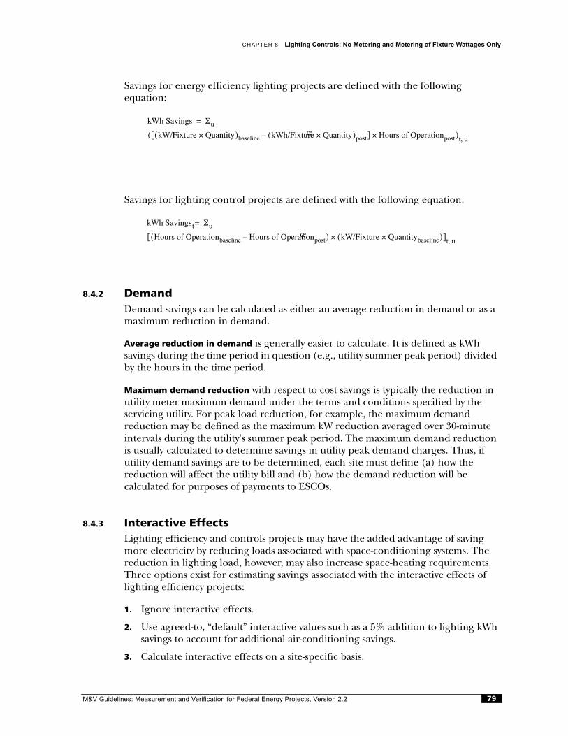
CHAPTER 8 Lighting Controls: No Metering and Metering of Fixture Wattages Only
Savings for energy efficiency lighting projects are defined with the followingequation:
Savings for lighting control projects are defined with the following equation:
8.4.2 Demand Demand savings can be calculated as either an average reduction in demand or as a maximum reduction in demand.
Average reduction in demand is generally easier to calculate. It is defined as kWhsavings during the time period in question (e.g., utility summer peak period) divided by the hours in the time period.
Maximum demand reduction with respect to cost savings is typically the reduction in utility meter maximum demand under the terms and conditions specified by theservicing utility. For peak load reduction, for example, the maximum demandreduction may be defined as the maximum kW reduction averaged over 30-minute intervals during the utility's summer peak period. The maximum demand reduction is usually calculated to determine savings in utility peak demand charges. Thus, if utility demand savings are to be determined, each site must define (a) how the reduction will affect the utility bill and (b) how the demand reduction will becalculated for purposes of payments to ESCOs.
8.4.3 Interactive EffectsLighting efficiency and controls projects may have the added advantage of saving more electricity by reducing loads associated with space-conditioning systems. The reduction in lighting load, however, may also increase space-heating requirements. Three options exist for estimating savings associated with the interactive effects of lighting efficiency projects:
1. Ignore interactive effects.
2. Use agreed-to, “default” interactive values such as a 5% addition to lighting kWh savings to account for additional air-conditioning savings.
3. Calculate interactive effects on a site-specific basis.
kWh Savings Σu
kW/Fixture Quantity×( )baseline kWh/Fixture Quantity×( )post–[ ] Hours of Operationpost×( )t u,œ
=
kWh Savingst Σu
Hours of Operationbaseline Hours of Operationpost–( ) kW/Fixture Quantitybaseline×( )×[ ]t u,œ
=
M&V Guidelines: Measurement and Verification for Federal Energy Projects, Version 2.2 79
SECTION I I I Selected M&V Methods Option A
8.5 Pre- and Post-Installation Submittals
For each site, the ESCO submits a project pre-installation report that includes thefollowing:
• A project description and schedule
• A pre-installation equipment survey
• Estimates of energy savings
• Documentation on utility billing data
• Projected budget
• Scheduled M&V activities.
If the federal agency defines the baseline condition, the ESCO must verify anagreed-to pre-installation equipment survey.
The ESCO submits a project post-installation report after the project is completed and defines projected energy savings for the first year. In addition, the report includes most of the components of the project pre-installation report, as well as information on actual rather than expected results of ECM installations.
8.6 Site-Specific Measurement and Verification Plan
The site-specific measurement and verification approach may be prespecified in the ESPC between the federal agency and the ESCO and/or agreed to after the award of the project. In either case, before the federal agency approves project construction, the ESCO must submit a final M&V plan that addresses the following elements on a site-specific basis:
• Overview of approach
• Specification of savings calculations
• Identification of corresponding variables and specification of assumptions
• Identification of data sources and/or collection techniques
• Specification of data collection (i.e., sampling, site inspection, and monitoring plan), if required
• Identification and resolution of any other M&V issues.
Specific M&V issues related to lighting efficiency and controls projects that must be addressed include the following:
• Decision whether to establish baseline fixture wattages at current efficiencystandards
M&V Guidelines: Measurement and Verification for Federal Energy Projects, Version 2.280

CHAPTER 8 Lighting Controls: No Metering and Metering of Fixture Wattages Only
• Avoidance of double-counting the savings from energy-efficiency projects that are controlled
• Designation of usage groups for defining stipulated lighting operating hours
• Assessment of non-operating fixtures
• Choice of methods to account for changes to baseline and post-installationfixture counts and types due to remodels
• Identification of interactive impact approach.
In addition, project pre- and post-installation reports should identify the specific steps required to implement the M&V plan.
M&V Guidelines: Measurement and Verification for Federal Energy Projects, Version 2.2 81
9Methods:
CLM-A-01
Constant-Speed Motor Efficiency: Metering of Motor kW
9.1 ECM Definition
Constant-speed motor efficiency projects involve the replacement of existing(baseline) motors with high-efficiency motors that serve constant-load systems. These ECMs are called constant-load motor efficiency projects because the power draw of the motors does not vary over time. These projects reduce demand and energy use.
This M&V method is appropriate only for projects where constant-load motors are replaced with similar capacity constant-speed motors, with two exceptions:
• Baseline motors may be replaced with smaller high-efficiency motors when the original motor was oversized for the load.
• Constant-speed motor drives may be adjusted to account for the difference in slip between the baseline motor and the high-efficiency motor.
If motor changes are accompanied by a change in operating schedule, a change in flow rate, or the installation of variable-speed drives, other M&V methods will be more appropriate.
9.2 Overview of Verification Method
Under Option A, Method CLM-A-01 is the only specified technique for verifyingconstant-load motor efficiency projects. This method assumes that the federal agency and the ESCO are confident that the motors operate at a consistent load with a definable operating schedule that can be stipulated.
Surveys are required to document existing (baseline) and new (post-installation) motors. The surveys should include (in a set format) the following data for each motor:
• Nameplate data
• Operating schedule
• Spot metering data
M&V Guidelines: Measurement and Verification for Federal Energy Projects, Version 2.282
CHAPTER 9 Constant-Speed Motor Efficiency: Metering of Motor kW
• Motor application
• Location.
Metering is required on at least a sample of motors to determine the average power draw for baseline and new motors. Demand savings are based on the average kW measured before new motors are installed minus the average kW measured after the new motors are installed. Allowances for differences in motor slip between existing and new motors may be allowed. Baseline and post-installation hours of operation, used in calculating energy savings, will be stipulated.
9.3 Calculation of Demand and Energy Savings
9.3.1 Baseline DemandThe baseline conditions identified in the pre-installation equipment survey will be defined by either the federal agency or the ESCO. If the baseline is defined by the federal agency, the ESCO will have an opportunity to verify the baseline. If thebaseline is defined by the ESCO, the federal agency will verify the baseline.
Steps involved in establishing the baseline demand are as follows:
• Conduct a pre-installation equipment survey
• Spot metering of existing motors.
Pre-Installation Equipment SurveyIn the pre-installation equipment survey, the equipment to be changed and the replacement equipment to be installed will be inventoried. Motor surveys withlocation information and corresponding building floor plans should be included with the survey submittal. The surveys will include, in a set format, nameplate data, motor horsepower, load served, operating schedule, spot metering data, motorapplication, and location.
Sample survey forms are included in Appendix B. Table M1 is the pre-installation survey form.
Spot Metering of Existing MotorsInstantaneous measurements of three-phase amps, volts, pava factor (PF), kVA, kW, and motor speed in RPM should be recorded based on spot metering of each motor to be replaced. These data should be entered into a form such as the one shown in Table M2 (Appendix B). Such measurements should be made using a true RMS meter with an accuracy at or approaching ±1% of reading.1 Other factors to measure include motor speed in RPM and the working fluid temperature if the motor serves a fan or pump. The temperature measurement may be taken at either the inlet oroutlet of the device, as long as such location is identical for the baseline and post-installation measurements.
M&V Guidelines: Measurement and Verification for Federal Energy Projects, Version 2.2 83
SECTION I I I Selected M&V Methods Option A
9.3.2 Adjustments to Baseline DemandBefore new motors are installed, adjustments to the baseline demand may be required for non-operating motors that are normally operating or intended foroperation. In addition, after ECM installation, adjustments to baseline demand may be required owing to factors such as remodeling or changes in occupancy. Methods for making adjustments should be specified in the site-specific M&V plan.
With respect to non-operating equipment, the party responsible for defining the baseline will also identify any non-operating motors. Non-operating equipment is equipment that is typically operating but that has broken parts and is intended for repair.
9.3.3 Post-Installation DemandThe new equipment will be defined and surveyed by the ESCO and verified by the federal agency. The ESCO should enter the information in Table M1. After high-efficiency motors are installed, spot metering will be conducted for all motors using the same meter and procedures used for the baseline motors. The results are entered in Table M2. See Section 8.3.1.
9.3.4 Changes in Load Factor (Slip)Standard-efficiency motors and high-efficiency motors may rotate at different rates when serving the same load. Such differences in rotational speed, characterized as “slip,” may lead to smaller savings than expected. Considerable impacts on savings due to slip may be reflected in the difference in load factor between the existing motor and a new high-efficiency motor. Large differences in load factor between the existing motor and the replacement high-efficiency motor may be symptomatic of other problems as well. As such, the ESCO will identify motors for which thedifference in load factor between the high-efficiency motor and the baseline motor is greater than 10%. If the load factor is outside that range, the ESCO will provide an explanation, with supporting calculations and documentation. An acceptable reason for changes in load factor greater than 10% may be that the high-efficiency motor is smaller than the original baseline motor.
9.3.5 Operating HoursOperating hours will be stipulated and agreed to by the federal agency and the ESCO. Sources of stipulated hours can be any of the following:
• Operation logs or documentation schedules from energy management systems
• Pre-metering of representative areas by the ESCO or federal agency
1. Report that, on the average, for all qualifying motors, the change in efficiency between a standard-effi-ciency motor and a high-efficiency motor, including an adjustment for slip, is 4.4%. As such, the resolu-tion of meters used to measure instantaneous kW should be much smaller than 4.0%. Gordon et al. (Gordon, F.M. et al. “Impacts of Performance Factors on Savings From Motor Replacement and New Motor Programs.” ACEEE 1994 Summer Study on Energy Efficiency in Buildings. American Council for an Energy-Efficient Economy. 1994.)
M&V Guidelines: Measurement and Verification for Federal Energy Projects, Version 2.284
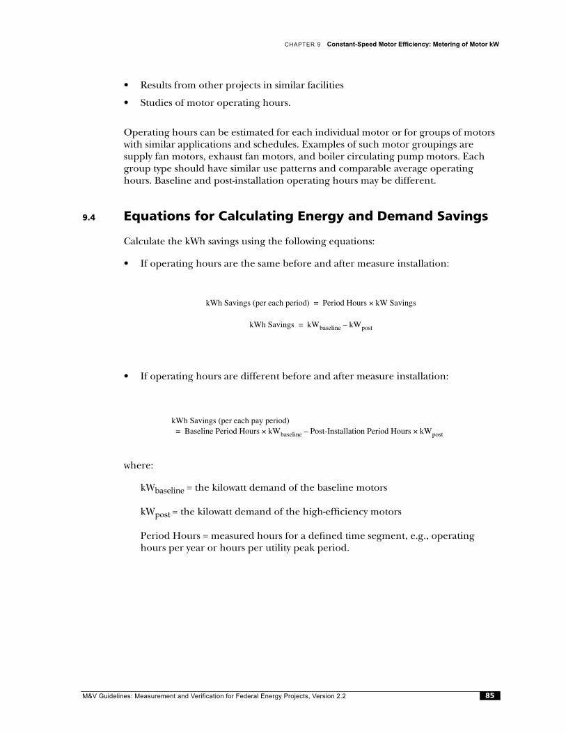
CHAPTER 9 Constant-Speed Motor Efficiency: Metering of Motor kW
• Results from other projects in similar facilities
• Studies of motor operating hours.
Operating hours can be estimated for each individual motor or for groups of motors with similar applications and schedules. Examples of such motor groupings aresupply fan motors, exhaust fan motors, and boiler circulating pump motors. Each group type should have similar use patterns and comparable average operating hours. Baseline and post-installation operating hours may be different.
9.4 Equations for Calculating Energy and Demand Savings
Calculate the kWh savings using the following equations:
• If operating hours are the same before and after measure installation:
• If operating hours are different before and after measure installation:
where:
kWbaseline = the kilowatt demand of the baseline motors
kWpost = the kilowatt demand of the high-efficiency motors
Period Hours = measured hours for a defined time segment, e.g., operating hours per year or hours per utility peak period.
kWh Savings (per each period) Period Hours kW Savings×=
kWh Savings kWbaseline kWpost–=
kWh Savings (per each pay period)Baseline Period Hours kWbaseline× Post-Installation Period Hours kWpost×–=
M&V Guidelines: Measurement and Verification for Federal Energy Projects, Version 2.2 85
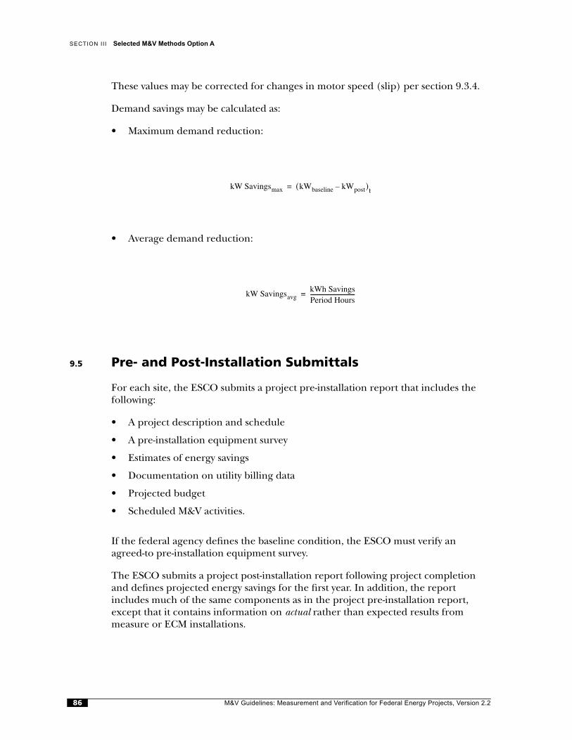
SECTION I I I Selected M&V Methods Option A
These values may be corrected for changes in motor speed (slip) per section 9.3.4.
Demand savings may be calculated as:
• Maximum demand reduction:
• Average demand reduction:
9.5 Pre- and Post-Installation Submittals
For each site, the ESCO submits a project pre-installation report that includes the following:
• A project description and schedule
• A pre-installation equipment survey
• Estimates of energy savings
• Documentation on utility billing data
• Projected budget
• Scheduled M&V activities.
If the federal agency defines the baseline condition, the ESCO must verify anagreed-to pre-installation equipment survey.
The ESCO submits a project post-installation report following project completion and defines projected energy savings for the first year. In addition, the report includes much of the same components as in the project pre-installation report, except that it contains information on actual rather than expected results frommeasure or ECM installations.
kW Savingsmax kWbaseline kWpost–( )t=
kW SavingsavgkWh SavingsPeriod Hours--------------------------------=
M&V Guidelines: Measurement and Verification for Federal Energy Projects, Version 2.286

CHAPTER 9 Constant-Speed Motor Efficiency: Metering of Motor kW
9.6 Site-Specific Measurement and Verification Plan
The site-specific measurement and verification approach may be prespecified in the ESPC contract between the federal agency and the ESCO and/or agreed to after the award of the project. In either case, before the federal agency approves the project construction, the ESCO must submit a final M&V plan that addresses the site-specific nature of the following elements:
• Overview of approach
• Specification of savings calculations
• Source of stipulated motor operating hours
• Specification of data collection methods, schedule, duration, equipment, and reporting format
• Identification and resolution of any other M&V issues.
Specific M&V issues that may need to be addressed and that are related to constant-load motor efficiency projects include the following:
• Operating hours for motors
• Assessment of non-operating motors
• Method(s) to account for changes in motor loading (slip) between baseline and new motors.
M&V Guidelines: Measurement and Verification for Federal Energy Projects, Version 2.2 87
10
Methods:
VSD-A-01
Variable-Speed Drive Motor Efficiency: Metering of Motor kW
10.1 ECM Definition
Variable-speed drive motor efficiency projects involve the replacement of constant-speed (baseline) motor controllers with variable-speed drive (or VSD) motorcontrollers. These projects reduce demand and energy use but do not necessarily reduce utility demand charges. Often VSD retrofits also include installation of new, high-efficiency motors. Typical VSD applications include HVAC fans and boiler and chiller circulating pumps.
This M&V method is appropriate only for VSD projects in which, for the baseline and post-installation motors, the following apply:
• Electrical demand varies as a function of operating scenarios—e.g., damperposition for baseline or motor speed for post-installation; the electrical demand for each operating scenario can be defined with spot measurements of motor power draw.
• Operating hours as a function of operating scenario can be stipulated.
If the affected motor has a complex variable load profile and/or a complicatedoperating schedule, other M&V methods will be more appropriate.
10.2 Overview of Verification Method
Under Option A, method VSD-A-01 is the only specified technique for verifying VSD projects. This method assumes that the federal agency and the ESCO are confident that the affected motors operate with a definable operating schedule that can bestipulated.
Surveys are required to document existing (baseline) and new (post-installation) motors and motor controls (e.g., motor starters, inlet vane dampers, and VSDs).The surveys should include (in a set format) the following data for each motor andcontrol device:
• Nameplate data
• Operating schedule
M&V Guidelines: Measurement and Verification for Federal Energy Projects, Version 2.288
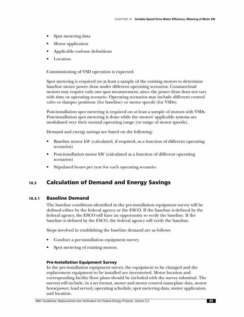
CHAPTER 10 Variable-Speed Drive Motor Efficiency: Metering of Motor kW
M&V Guidelines: Measurement and Verification for Federal Energy Projects, Version 2.2 89
• Spot metering data
• Motor application
• Applicable end-use definitions
• Location.
Commissioning of VSD operation is expected.
Spot metering is required on at least a sample of the existing motors to determine baseline motor power draw under different operating scenarios. Constant-load motors may require only one spot measurement, since the power draw does not vary with time or operating scenario. Operating scenarios may include different control valve or damper positions (for baseline) or motor speeds (for VSDs).
Post-installation spot metering is required on at least a sample of motors with VSDs. Post-installation spot metering is done while the motors' applicable systems aremodulated over their normal operating range (or range of motor speeds).
Demand and energy savings are based on the following:
• Baseline motor kW (calculated, if required, as a function of different operating scenarios)
• Post-installation motor kW (calculated as a function of different operatingscenarios)
• Stipulated hours per year for each operating scenario.
10.3 Calculation of Demand and Energy Savings
10.3.1 Baseline DemandThe baseline conditions identified in the pre-installation equipment survey will be defined either by the federal agency or the ESCO. If the baseline is defined by the federal agency, the ESCO will have an opportunity to verify the baseline. If thebaseline is defined by the ESCO, the federal agency will verify the baseline.
Steps involved in establishing the baseline demand are as follows:
• Conduct a pre-installation equipment survey.
• Spot metering of existing motors.
Pre-Installation Equipment SurveyIn the pre-installation equipment survey, the equipment to be changed and the replacement equipment to be installed are inventoried. Motor location andcorresponding facility floor plans should be included with the survey submittal. The surveys will include, in a set format, motor and motor control nameplate data, motor horsepower, load served, operating schedule, spot metering data, motor application, and location.
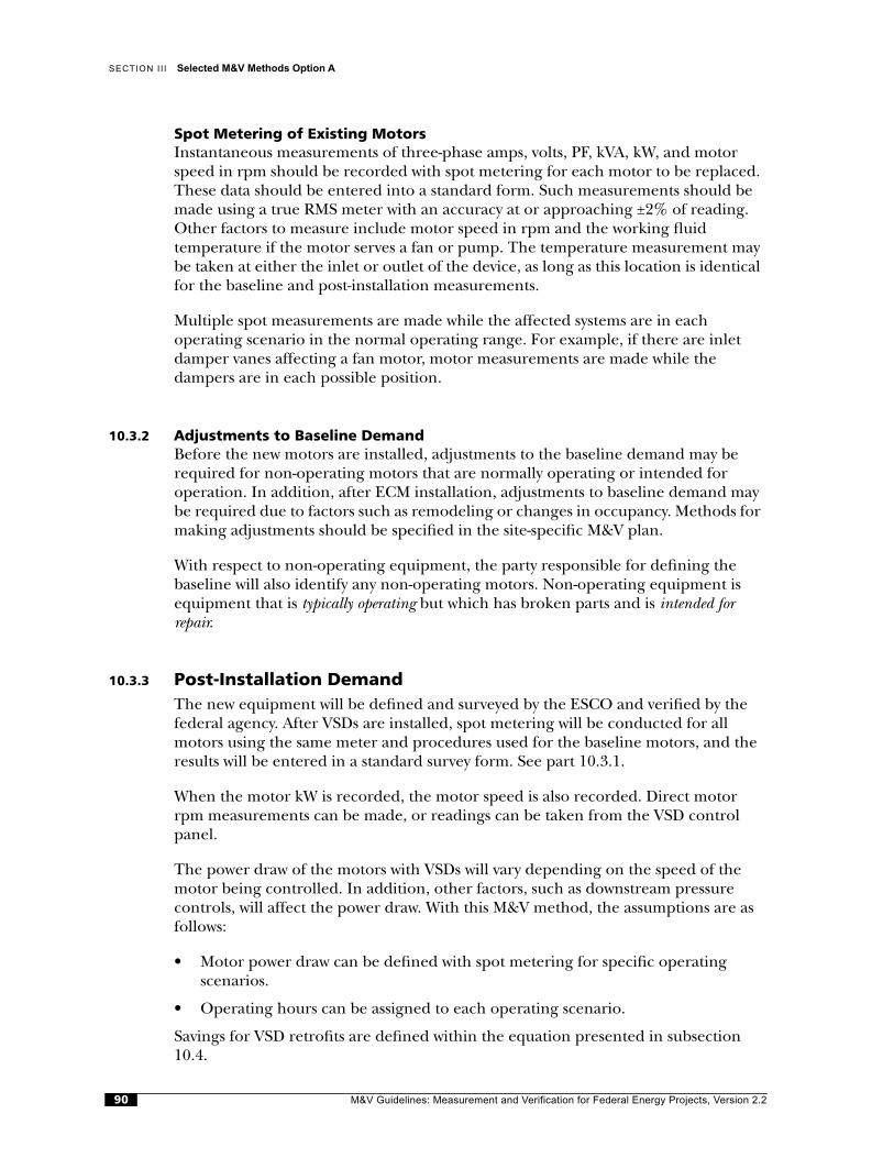
SECTION I I I Selected M&V Methods Option A
Spot Metering of Existing MotorsInstantaneous measurements of three-phase amps, volts, PF, kVA, kW, and motor speed in rpm should be recorded with spot metering for each motor to be replaced. These data should be entered into a standard form. Such measurements should be made using a true RMS meter with an accuracy at or approaching ±2% of reading. Other factors to measure include motor speed in rpm and the working fluidtemperature if the motor serves a fan or pump. The temperature measurement may be taken at either the inlet or outlet of the device, as long as this location is identical for the baseline and post-installation measurements.
Multiple spot measurements are made while the affected systems are in eachoperating scenario in the normal operating range. For example, if there are inlet damper vanes affecting a fan motor, motor measurements are made while thedampers are in each possible position.
10.3.2 Adjustments to Baseline DemandBefore the new motors are installed, adjustments to the baseline demand may be required for non-operating motors that are normally operating or intended foroperation. In addition, after ECM installation, adjustments to baseline demand may be required due to factors such as remodeling or changes in occupancy. Methods for making adjustments should be specified in the site-specific M&V plan.
With respect to non-operating equipment, the party responsible for defining the baseline will also identify any non-operating motors. Non-operating equipment is equipment that is typically operating but which has broken parts and is intended for repair.
10.3.3 Post-Installation DemandThe new equipment will be defined and surveyed by the ESCO and verified by the federal agency. After VSDs are installed, spot metering will be conducted for all motors using the same meter and procedures used for the baseline motors, and the results will be entered in a standard survey form. See part 10.3.1.
When the motor kW is recorded, the motor speed is also recorded. Direct motor rpm measurements can be made, or readings can be taken from the VSD control panel.
The power draw of the motors with VSDs will vary depending on the speed of the motor being controlled. In addition, other factors, such as downstream pressurecontrols, will affect the power draw. With this M&V method, the assumptions are as follows:
• Motor power draw can be defined with spot metering for specific operatingscenarios.
• Operating hours can be assigned to each operating scenario.
Savings for VSD retrofits are defined within the equation presented in subsection 10.4.
M&V Guidelines: Measurement and Verification for Federal Energy Projects, Version 2.290
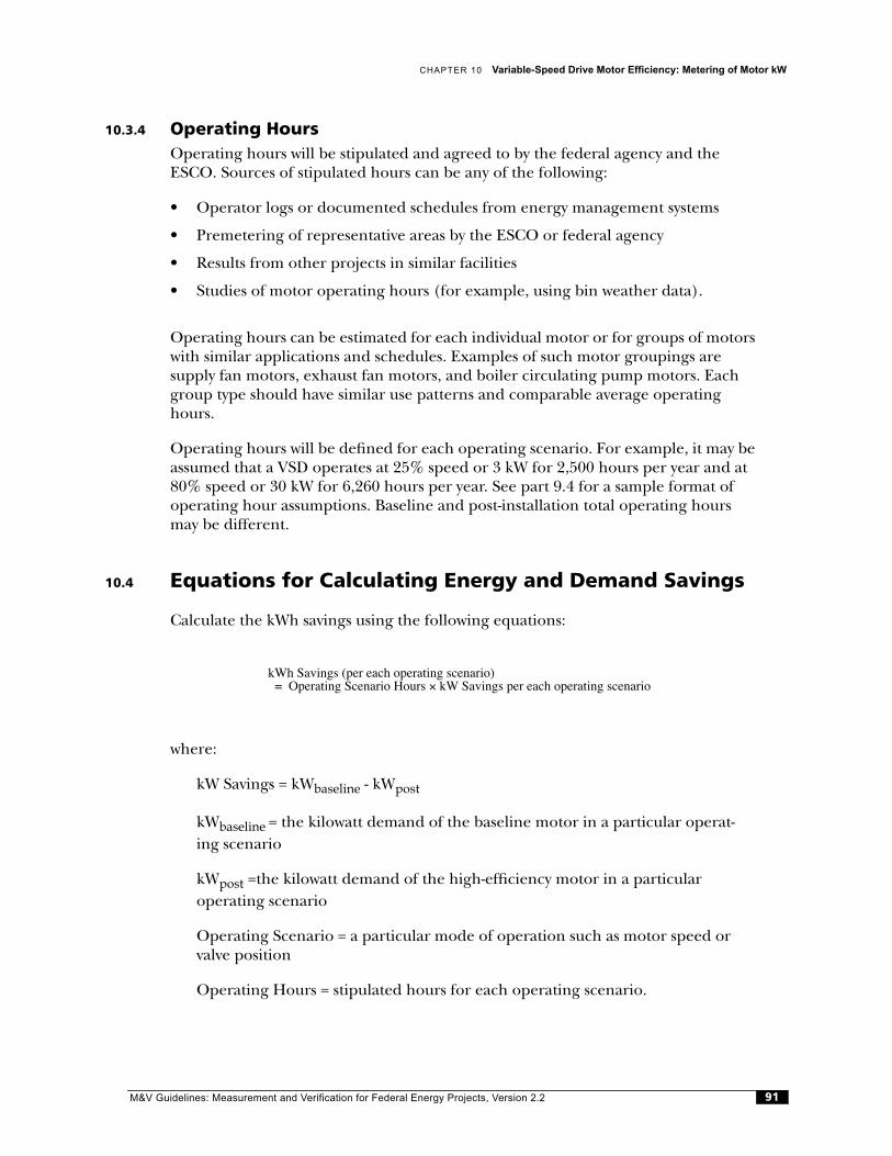
CHAPTER 10 Variable-Speed Drive Motor Efficiency: Metering of Motor kW
10.3.4 Operating HoursOperating hours will be stipulated and agreed to by the federal agency and the ESCO. Sources of stipulated hours can be any of the following:
• Operator logs or documented schedules from energy management systems
• Premetering of representative areas by the ESCO or federal agency
• Results from other projects in similar facilities
• Studies of motor operating hours (for example, using bin weather data).
Operating hours can be estimated for each individual motor or for groups of motors with similar applications and schedules. Examples of such motor groupings aresupply fan motors, exhaust fan motors, and boiler circulating pump motors. Each group type should have similar use patterns and comparable average operating hours.
Operating hours will be defined for each operating scenario. For example, it may be assumed that a VSD operates at 25% speed or 3 kW for 2,500 hours per year and at 80% speed or 30 kW for 6,260 hours per year. See part 9.4 for a sample format of operating hour assumptions. Baseline and post-installation total operating hours may be different.
10.4 Equations for Calculating Energy and Demand Savings
Calculate the kWh savings using the following equations:
where:
kW Savings = kWbaseline - kWpost
kWbaseline = the kilowatt demand of the baseline motor in a particular operat-ing scenario
kWpost =the kilowatt demand of the high-efficiency motor in a particular operating scenario
Operating Scenario = a particular mode of operation such as motor speed or valve position
Operating Hours = stipulated hours for each operating scenario.
kWh Savings (per each operating scenario)Operating Scenario Hours kW Savings per each operating scenario×=
M&V Guidelines: Measurement and Verification for Federal Energy Projects, Version 2.2 91
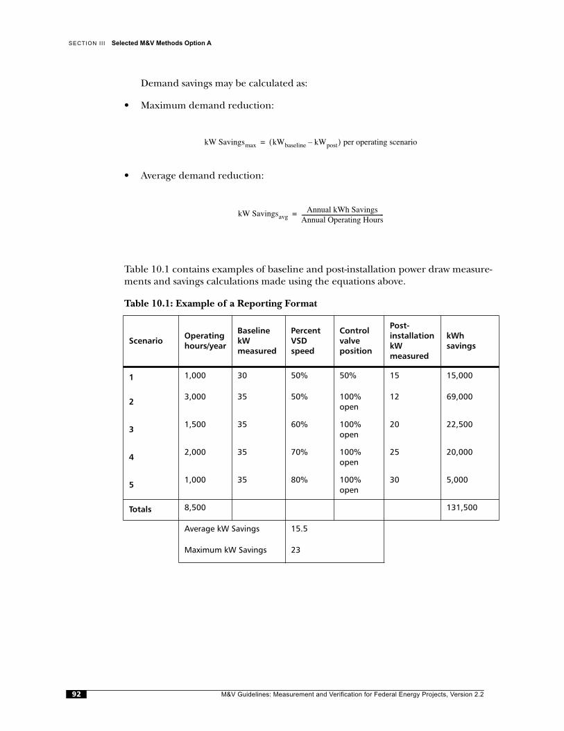
SECTION I I I Selected M&V Methods Option A
9
Demand savings may be calculated as:
• Maximum demand reduction:
• Average demand reduction:
Table 10.1 contains examples of baseline and post-installation power draw measure-ments and savings calculations made using the equations above.
Table 10.1: Example of a Reporting Format
ScenarioOperating hours/year
Baseline kW measured
Percent VSD speed
Control valve position
Post-installation kW measured
kWh savings
1 1,000 30 50% 50% 15 15,000
23,000 35 50% 100%
open12 69,000
31,500 35 60% 100%
open20 22,500
42,000 35 70% 100%
open25 20,000
51,000 35 80% 100%
open30 5,000
Totals 8,500 131,500
Average kW Savings 15.5
Maximum kW Savings 23
kW Savingsmax kWbaseline kWpost–( ) per operating scenario=
kW SavingsavgAnnual kWh Savings
Annual Operating Hours-----------------------------------------------------------=
M&V Guidelines: Measurement and Verification for Federal Energy Projects, Version 2.22
CHAPTER 10 Variable-Speed Drive Motor Efficiency: Metering of Motor kW
10.5 Pre- and Post-Installation Submittals
For each site, the ESCO submits a project pre-installation report that includes the following:
• A project description and schedule
• A pre-installation equipment survey
• Estimates of energy savings
• Documentation on utility billing data
• Projected budget
• Scheduled M&V activities.
If the federal agency defines the baseline condition, the ESCO must verify anagreed-to pre-installation equipment survey.
The ESCO submits a project post-installation report following project completion and defines projected energy savings for the first year. In addition, the report includes most of the same components as the project pre-installation report, as well as information on actual rather than expected results from measure installations.
10.6 Site-Specific Measurement and Verification Plan
The site-specific measurement and verification approach may be prespecified in the ESPC between the federal agency and ESCO and/or agreed to after the award of the project. In either case, before the federal agency approves the project construction, the ESCO must submit a final M&V plan that addresses the following elements on a site-specific basis:
• Overview of approach
• Specification of savings calculations
• Source of stipulated motor operating hours
• Specification of data collection methods, schedule, duration, equipment, and reporting format
• Identification and resolution of any other M&V issues.
Specific M&V issues that may need to be addressed and that are related to VSD projects include the following:
• Definition of operating scenarios for motors
• Motor operating hours for each operating scenario
• Assessment of non-operating motors
• Meter specifications and spot metering methodology.
M&V Guidelines: Measurement and Verification for Federal Energy Projects, Version 2.2 93
11
Methods:
CH-A-01
CH-A-02
Chiller Replacement: No Metering and Verification of Chiller kW/ton Methods
11.1 ECM Definition
This ECM involves chillers used for space conditioning or process loads. Projects can include either of the following:
• Existing chillers replaced with more energy-efficient chillers
• Changes in chiller controls that improve chiller efficiency.
Two M&V methods are described in this chapter. For method CH-A-01, the chiller efficiency (e.g., kW per ton) and the chiller load (e.g., tons per year) are stipulated. For method CH-A-02, the chiller efficiency is measured and the chiller load isstipulated. Thus, these methods are appropriate only for projects in which the baseline and post-installation chiller efficiency and/or the chiller load can be defined and stipulated by the ESCO and the federal agency.
11.2 Overview of Verification Methods
Surveys are required to document existing (baseline) and new (post-installation) chillers and chiller auxiliaries (e.g., chilled water pumps and cooling towers). The surveys should include the following (in a set format) for each chiller and control device:
• Nameplate data
• Chiller application
• Operating schedules.
Commissioning of chiller operation is expected.
Method CH-A-01—No MeteringBaseline and post-installation chiller ratings (e.g., kW/ton or integrated part load value [IPLV]) are stipulated on the basis of manufacturers' or other data. Annual cooling loads (e.g., annual or monthly ton-hours) are also stipulated. Energy savings are based on the product of (a) the difference between average baseline kW/ton and post-installation kW/ton and (b) cooling load in ton-hours.
M&V Guidelines: Measurement and Verification for Federal Energy Projects, Version 2.294
CHAPTER 11 Chiller Replacement: No Metering and Verification of Chiller kW/ton Methods
Method CH-A-02—Performance MeasuredBaseline and post-installation chiller ratings (e.g., kW/ton, IPLV) are based on short-term metering of chiller kW (and perhaps auxiliary pump and cooling tower fan kW) and chiller load. Annual cooling loads (e.g., annual or monthly ton-hours) arestipulated. Energy savings are based on the product of (a) the difference between baseline kW/ton and post-installation kW/ton (possibly at each load rating) and(b) cooling load in ton-hours.
Methods CH-A-01 and CH-A-02 can be “mixed and matched” for the baseline chiller(s) and new chiller(s). For example, baseline chiller efficiency may bemeasured, and manufacturer's data can be used to stipulate performance ratingsfor the new chiller.
Baseline and post-installation chiller load can be different to account for changes in load during the term of the contract.
11.3 Calculation of Demand and Energy Savings
11.3.1 Baseline DemandThe baseline conditions identified in the pre-installation equipment survey will be defined by either the federal agency or the ESCO. If the baseline is defined by the federal agency, the ESCO will have the opportunity to verify the baseline. If thebaseline is defined by the ESCO, the federal agency will verify the baseline.
Steps involved in establishing the baseline demand are:
• Pre-installation equipment survey
• Defining chiller efficiency (method CH-A-01) or metering existing chillers (method CH-A-02).
Pre-Installation Equipment SurveyIn the pre-installation equipment survey, the equipment to be changed and the equipment to be installed will be inventoried. Chiller location and corresponding facility floor plans should be included with the survey submittal. The surveys will include, in a set format:
• Chiller and chiller auxiliaries nameplate data
• Chiller age, condition, and ratings
• Load served
• Operating schedule
• Chiller application
• Equipment locations.
M&V Guidelines: Measurement and Verification for Federal Energy Projects, Version 2.2 95
SECTION I I I Selected M&V Methods Option A
Method CH-A-01—Stipulated Chiller EfficienciesFor this simple M&V method, the chiller performance is stipulated—i.e., agreed to by the federal agency and the ESCO. The most common source of chillerperformance data is the manufacturer. For existing chillers, the “nameplate”performance ratings may be downgraded based on the chillers' age and/orcondition (e.g., fouling). Chiller efficiency can be presented in several formats, depending on the type of load data that will be stipulated. Possible options include annual average kW/ton, expressed as the IPLV or kW/ton per incremental cooling loads for the chiller(s) affected by the ECM.1
Method CH-A-02—Metering of Existing ChillersFor this M&V method, the baseline chiller efficiency is measured. The following data should be collected:
• Chiller kW
• Chilled water flow, entering and leaving temperatures for calculating cooling load
• Chiller circulating and condenser pumps kW (kWh) if they are to be replaced or modified
• Cooling tower fan(s) kW (kWh) if they are to be replaced or modified.2
These data should be entered into a standard form. Such measurements should be made using a meter with an accuracy at or approaching ±2% of reading.
Multiple measurements are made while the cooling systems are operating atdifferent loads so that the complete range of chiller performance can be evaluated. Optimally, baseline metering is performed during a period where a range of cooling loads exist (e.g., summer).
ASHRAE is preparing chiller measurement protocols (e.g., RP-827) that may bespecified by the federal agency.
11.3.2 Post-Installation DemandThe new equipment will be defined and surveyed by the ESCO and verified by the federal agency.
1. For example, per the appropriate standards of the Air-Conditioning and Refrigeration Institute2. Condenser pumps and cooling tower measurements are not involved in air-cooled systems. Circulat-ing pump measurements are not involved in DX systems. Condenser flows and temperatures can also be measured to check system energy balances. For DX systems, air flows and temperatures (although more difficult than water system measurements) are measured to determine cooling load.
M&V Guidelines: Measurement and Verification for Federal Energy Projects, Version 2.296
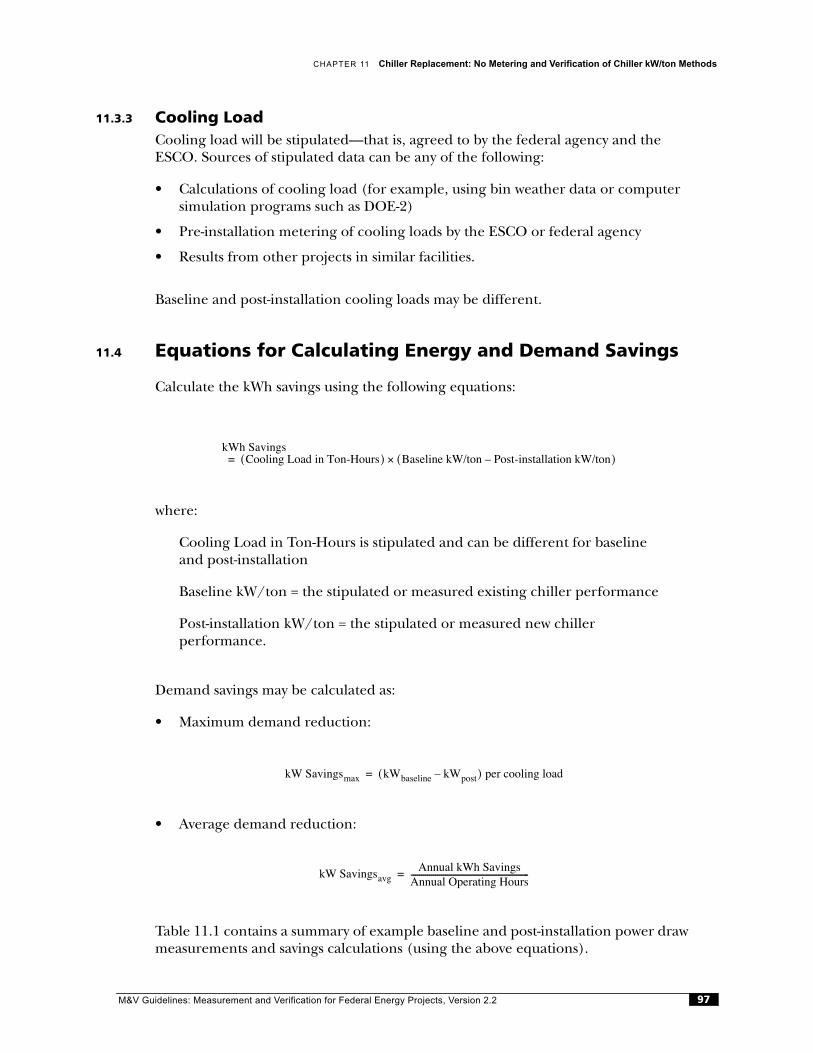
CHAPTER 11 Chiller Replacement: No Metering and Verification of Chiller kW/ton Methods
11.3.3 Cooling LoadCooling load will be stipulated—that is, agreed to by the federal agency and the ESCO. Sources of stipulated data can be any of the following:
• Calculations of cooling load (for example, using bin weather data or computer simulation programs such as DOE-2)
• Pre-installation metering of cooling loads by the ESCO or federal agency
• Results from other projects in similar facilities.
Baseline and post-installation cooling loads may be different.
11.4 Equations for Calculating Energy and Demand Savings
Calculate the kWh savings using the following equations:
where:
Cooling Load in Ton-Hours is stipulated and can be different for baseline and post-installation
Baseline kW/ton = the stipulated or measured existing chiller performance
Post-installation kW/ton = the stipulated or measured new chillerperformance.
Demand savings may be calculated as:
• Maximum demand reduction:
• Average demand reduction:
Table 11.1 contains a summary of example baseline and post-installation power draw measurements and savings calculations (using the above equations).
kWh SavingsCooling Load in Ton-Hours( ) Baseline kW/ton Post-installation kW/ton–( )×=
kW Savingsmax kWbaseline kWpost–( ) per cooling load=
kW SavingsavgAnnual kWh Savings
Annual Operating Hours-----------------------------------------------------------=
M&V Guidelines: Measurement and Verification for Federal Energy Projects, Version 2.2 97
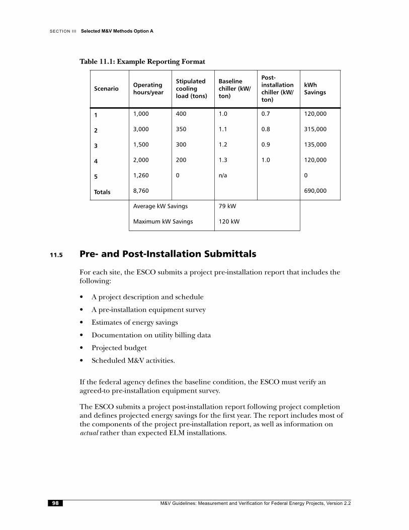
SECTION I I I Selected M&V Methods Option A
Table 11.1: Example Reporting Format
11.5 Pre- and Post-Installation Submittals
For each site, the ESCO submits a project pre-installation report that includes thefollowing:
• A project description and schedule
• A pre-installation equipment survey
• Estimates of energy savings
• Documentation on utility billing data
• Projected budget
• Scheduled M&V activities.
If the federal agency defines the baseline condition, the ESCO must verify anagreed-to pre-installation equipment survey.
The ESCO submits a project post-installation report following project completion and defines projected energy savings for the first year. The report includes most of the components of the project pre-installation report, as well as information on actual rather than expected ELM installations.
ScenarioOperating hours/year
Stipulated cooling load (tons)
Baseline chiller (kW/ton)
Post-installation chiller (kW/ton)
kWh Savings
1 1,000 400 1.0 0.7 120,000
2 3,000 350 1.1 0.8 315,000
3 1,500 300 1.2 0.9 135,000
4 2,000 200 1.3 1.0 120,000
5 1,260 0 n/a 0
Totals 8,760 690,000
Average kW Savings 79 kW
Maximum kW Savings 120 kW
M&V Guidelines: Measurement and Verification for Federal Energy Projects, Version 2.298
CHAPTER 11 Chiller Replacement: No Metering and Verification of Chiller kW/ton Methods
11.6 Site-Specific Measurement and Verification Plan
The site-specific measurement and verification approach may be prespecified in the ESPC between the federal agency and the ESCO and/or agreed to after the awardof the project. In either case, before the federal agency approves the projectconstruction, the ESCO must submit a final M&V plan that addresses the following elements on a site-specific basis:
• Overview of approach
• Specification of savings calculations
• Source of stipulated chiller performance and/or cooling loads
• Specification of data collection methods, schedule, duration, equipment, and reporting format
• Identification and resolution of any other M&V issues.
Specific M&V issues that must be addressed and that are related to chillerreplacement projects include the following:
• Definition of operating scenarios
• Cooling loads of the chillers at each operating mode
• Duration of monitoring.
M&V Guidelines: Measurement and Verification for Federal Energy Projects, Version 2.2 99

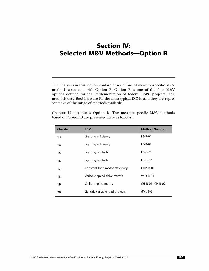
M&V Guidelines:
Section IV:Selected M&V Methods—Option B
The chapters in this section contain descriptions of measure-specific M&Vmethods associated with Option B. Option B is one of the four M&Voptions defined for the implementation of federal ESPC projects. Themethods described here are for the most typical ECMs, and they are repre-sentative of the range of methods available.
Chapter 12 introduces Option B. The measure-specific M&V methodsbased on Option B are presented here as follows:
Chapter ECM Method Number
13 Lighting efficiency LE-B-01
14 Lighting efficiency LE-B-02
15 Lighting controls LC-B-01
16 Lighting controls LC-B-02
17 Constant-load motor efficiency CLM-B-01
18 Variable-speed drive retrofit VSD-B-01
19 Chiller replacements CH-B-01, CH-B-02
20 Generic variable load projects GVL-B-01
Measurement and Verification for Federal Energy Projects, Version 2.2 101
12Introduction to Option B
Option B involves a retrofit or system-level M&V assessment. The approach is intended for retrofits with performance factors (e.g. end-use capacity, demand, power) and operational factors (lighting operational hours, cooling ton-hours) that can be measured at the component or system level. It is appropriate to use spot or short-term measurements to determine energy savings when variations in operations are not expected to change. When variations are expected, it is appropriate tomeasure factors continuously during the contract.
Option B is typically used when any or all of these conditions apply:
• For simple equipment-replacement projects with energy savings that are less than 20% of total facility energy use as recorded by the relevant utility meter orsub-meter.
• When energy savings values per individual measure are desired.
• When interactive effects are to be ignored or are stipulated using estimating methods that do not involve long-term measurements.
• When the independent variables that affect energy use are not complex and excessively difficult or expensive to monitor.
• When sub-meters already exist that record the energy use of subsystems under consideration (e.g., a 277 Volt lighting circuit or a separate submeter for HVAC systems).
12.1 Approach
Option B verification procedures involve the same items as Option A but generally involve more end-use metering. Option B relies on the physical assessment ofequipment change-outs to ensure the installation is to specification. The potential to generate savings is verified through observations, inspections, and spot/short-term/continuous metering. The continuous metering of one or more variables may only occur after retrofit installation. Spot or short-term metering may be sufficient to characterize the baseline condition.
M&V Guidelines: Measurement and Verification for Federal Energy Projects, Version 2.2102
CHAPTER 12 Introduction to Option B
12.2 M&V Considerations
Option B is for projects in which (a) the potential to generate savings must beverified and (b) actual energy use during the contract term needs to be measured for comparison with the baseline model for calculating savings. Option B involves procedures for verifying the same items as Option A, plus the determination of energy savings during the contract term through short-term or continuous end-use metering. Option B:
• Confirms that the proper equipment/systems were installed and that they have the potential to generate predicted savings.
• Determines an energy (and cost) savings value using short-term or continuous measurement of performance and operating factors.
All end-use technologies can be verified with Option B; however, the degree ofdifficulty and costs associated with verification increases as metering complexity increases. Energy savings accuracy is defined by the owner or is negotiated with the ESCO. The task of measuring or determining energy savings using Option B can be more difficult and costly than that of Option A. Results are typically more precise, however, than the use of stipulations as defined for Option A.
Methods involve the use of pre- and post-installation measurement of one or more variables. If operation does not vary between pre and post conditions, monitoring pre-installation operation is not necessary. Spot or short-term measurements offactors are appropriate when variations in loads and operation are not expected. When variations are expected, it is appropriate to measure factors continuously.Performing continuous measurements (i.e. periodic measurements taken over the term of the contract) account for operating variations and will result in closer approximations of actual energy savings. Continuous measurements provide long-term persistence data on the energy use of the equipment or system. These data can be used to improve or optimize the operation of the equipment on a real-time basis, thereby improving the benefit of the retrofit. In situations like constant-loadretrofits, however, there may be no inherent benefit of continuous over short-term measurements. Measurement of all affected pieces of equipment or systems may not be required if statistically valid sampling is used. For example, population samples may be measured to estimate operating hours for a selected group of lightingfixtures or the power draw of certain constant-load motors that have beenpredetermined to operate in a similar manner.
M&V Guidelines: Measurement and Verification for Federal Energy Projects, Version 2.2 103

13Methods:
LE-B-01
Lighting Efficiency: Monitoring of Operating Hours
13.1 Project Definition
The lighting projects covered by this verification plan are as follows:
• Retrofits of existing fixtures, lamps, and/or ballasts with an identical number of more energy-efficient fixtures, lamps, and/or ballasts
• De-lamping with or without the use of reflectors.
These lighting efficiency projects reduce demand; however, the fixtures have the same pre- and post-retrofit operating hours.
13.2 Overview of Verification Method
This method is similar to Option A methods LE-A-01 and LE-A-02 in that surveyswill be made of all baseline and post-installation lighting fixtures and that fixture wattages will be based on a standard table or measurements. This method differs in that, instead of stipulating operating hours, the operating hours are measured throughout the term of the agreement, either at regular intervals or continuously.
Surveys are required of existing (baseline) and new (post-installation) fixtures.Corrections may be required for non-operating fixtures. Light level requirements may be specified for projects that involve reducing lighting levels.
Fixture wattages will be determined from any of the following:
• A table of standard wattages
• Documentation on each fixture or ballast or lamp combination
• Measurements of representative fixtures or lighting circuits.
Post-installation hours of operation will be determined by monitoring a statistically valid sample of fixtures and rooms. The monitoring time period must be reasonable and account for any seasonal variations.
M&V Guidelines: Measurement and Verification for Federal Energy Projects, Version 2.2104
CHAPTER 13 Lighting Efficiency: Monitoring of Operating Hours
This chapter addresses one of two M&V methods under Option B for lightingefficiency projects. Method LE-B-01 requires pre- and post-installation equipment surveys in combination with post-installation metering of hours of operation toestimate savings. Chapter 11 addresses Method LE-B-02, which involves baseline and post-installation lighting circuit measurements to determine both demand and energy savings.
13.3 Calculating Demand and Energy Savings
13.3.1 Baseline DemandThe baseline conditions identified in the pre-installation equipment survey may be defined by either the federal agency or the ESCO. If the baseline is defined by the federal agency, the ESCO will have an opportunity to verify the baseline. If thebaseline is defined by the ESCO, the federal agency will verify the baseline.
In the pre-installation equipment survey, the equipment to be changed and the replacement equipment to be installed will be inventoried. Room location andcorresponding building floor plans should be included with the survey submittal. The surveys will include, in a set format, fixture, lamp, and ballast types; usage area designations; counts of operating and non-operating fixtures; and whether the room is air-conditioned and/or heated.
Fixture wattages will be based on a table of standard fixture wattages or spot/short-term metering.
Wattage TableFixture wattages will be from a standard table unless other documentation isprovided. A standard table of fixture wattages should contain common lamp andballast combinations. In the event that a fixture is not in the table, the partyconducting the pre-installation equipment survey should either (a) take wattage measurements for a representative sample of fixtures or (b) provide a documented source of the fixture wattages for approval by the other party.
In general, a standard table of fixture wattages should be used for the baselinefixtures, and documented manufacturers' data should be used for post-installation fixtures.
Fixture Wattage Metering Fixture wattages will be measured. An example of a metering protocol is as follows:
The ESCO will take 15-minute, true RMS wattage measurements from at least six fixtures representative of the baseline and post-installation fixtures (actual values may vary by application). Readings will be averaged to determine per-fixture wattage values. For post-installation fixtures, readings should be taken only after the new fixtures have been operating for at least 100 hours. Meters used for this task will be calibrated and have an accuracy of ±2% of reading or better.
M&V Guidelines: Measurement and Verification for Federal Energy Projects, Version 2.2 105
SECTION IV Selected M&V Methods Option B
13.3.2 Adjustments to Baseline DemandBefore the new lighting fixtures are installed, adjustments to the baseline demand may be required for non-operating fixtures. In addition, after ECM installation, adjustments to baseline demand may be required because of remodeling orchanges in occupancy. Methods for making adjustments should be specified in the site-specific M&V plan.
With respect to non-operating fixtures, the party responsible for defining thebaseline will also identify any non-operating fixtures. Non-operating fixtures are those that are typically operating but that have broken lamps, ballasts, and/or switches that are intended for repair.
A de-lamped fixture is not a non-operating fixture; thus, de-lamped fixtures should have their own unique wattage designations. Fixtures that have been disabled orde-lamped or that are broken and not intended for repair should not be included in the calculation of baseline demand or energy. They should, however, be noted in the lighting survey to avoid confusion.
For non-operating fixtures, the baseline demand may be adjusted by using values from the standard table of fixture wattages or from fixture wattage measurements. The adjustment for non-operating fixtures will be limited to a percentage of the total fixture count per facility, e.g., 10%. If, for example, more than 10% of the total number offixtures are non-operating, the number of fixtures beyond 10% will be assumed to have a baseline fixture wattage of zero.
13.3.3 Post-Installation DemandThe post-installation conditions identified in the post-installation equipment survey will be defined by the ESCO and verified by the federal agency. The techniquesdiscussed in part 13.3.1 can be used to inventory the installed equipment.
13.3.4 Operating HoursTo measure post-installation operating hours, three key issues must be defined:
1. The appropriate usage groups and sample sizes for metering each facility or group of similar facilities.
2. Whether lighting circuit measurements or lighting loggers will be used.
3. How long operating hours will be metered to determine a representativeoperating profile.
Usage GroupsBuilding usage areas will be identified for areas with comparable average operating hours, as determined by the lights operating during the year or by each of theelectric utility's costing periods. Usage areas must be defined in a way that groups together areas that have similar occupancies and lighting operating-hour schedules.
M&V Guidelines: Measurement and Verification for Federal Energy Projects, Version 2.2106

CHAPTER 13 Lighting Efficiency: Monitoring of Operating Hours
For each unique usage area, the ESCO or federal agency will develop a sampling plan to monitor the average operating hours of either a sample of fixtures or asample of circuits. Sampling guidelines are in Appendix D.
MetersThe ESCO will specify the meter to be used in the site-specific M&V plan.Measurements of operating hours are typically done with either of these:
• “Light loggers,” which are devices that measure the operating hours of individual fixtures through the use of photocells. A wide variety of products are available that store information that can be translated into either elapsed run times forfixtures (run-time loggers) or actual load profiles of on and off times for fixtures (time-of-use loggers)
• Current or power measurements of lighting circuits that, when calibrated to the total connected lighting load on the circuit, can be used to determine how many fixtures were operating in terms of elapsed time or actual time-of-use loadprofiles.
The meter and recording device may be required to measure and record dataindicating operating hours for each all-utility time-of-use costing period. The ESCO must use a data logger that records status at frequent intervals (i.e., at least every 15 minutes). “Raw” as well as “compiled” data from the meter(s) must be madeavailable.
If the ESCO chooses to monitor circuits to determine average operating hours, the ESCO will use run-time or power recording meters that record the circuit on/offpattern in each utility costing period. The ESCO will not monitor circuits when the circuit serving the lighting retrofit load also serves other non lighting loads thatcannot be distinguished from the lighting load. Thus, only when lighting andnon-lighting loads are separable may circuits be monitored.
Period of MonitoringMonitoring provides an estimate of annual equipment operating hours. Theduration and timing of the installation of run-time monitoring have a stronginfluence on the accuracy of operating-hours estimates. Monitoring equipment should not be installed during significant holiday or vacation periods. If a holiday or vacation falls within the monitoring installation period, that period should be extended for the same number of days as the holiday or vacation.
If less than continuous monitoring is used, the lighting operating hours during the monitored period will be extrapolated to the full year. A minimum monitoring period of three weeks is recommended for almost all usage-area groups. For situations in which lighting might vary seasonally, such as classrooms, or according to ascheduled activity, it may be necessary to determine lighting operating hours duringdifferent times of the year.
The ESCO-supplied site-specific M&V plan will include the detailed the agreed-to sample plan and monitoring plan.
M&V Guidelines: Measurement and Verification for Federal Energy Projects, Version 2.2 107
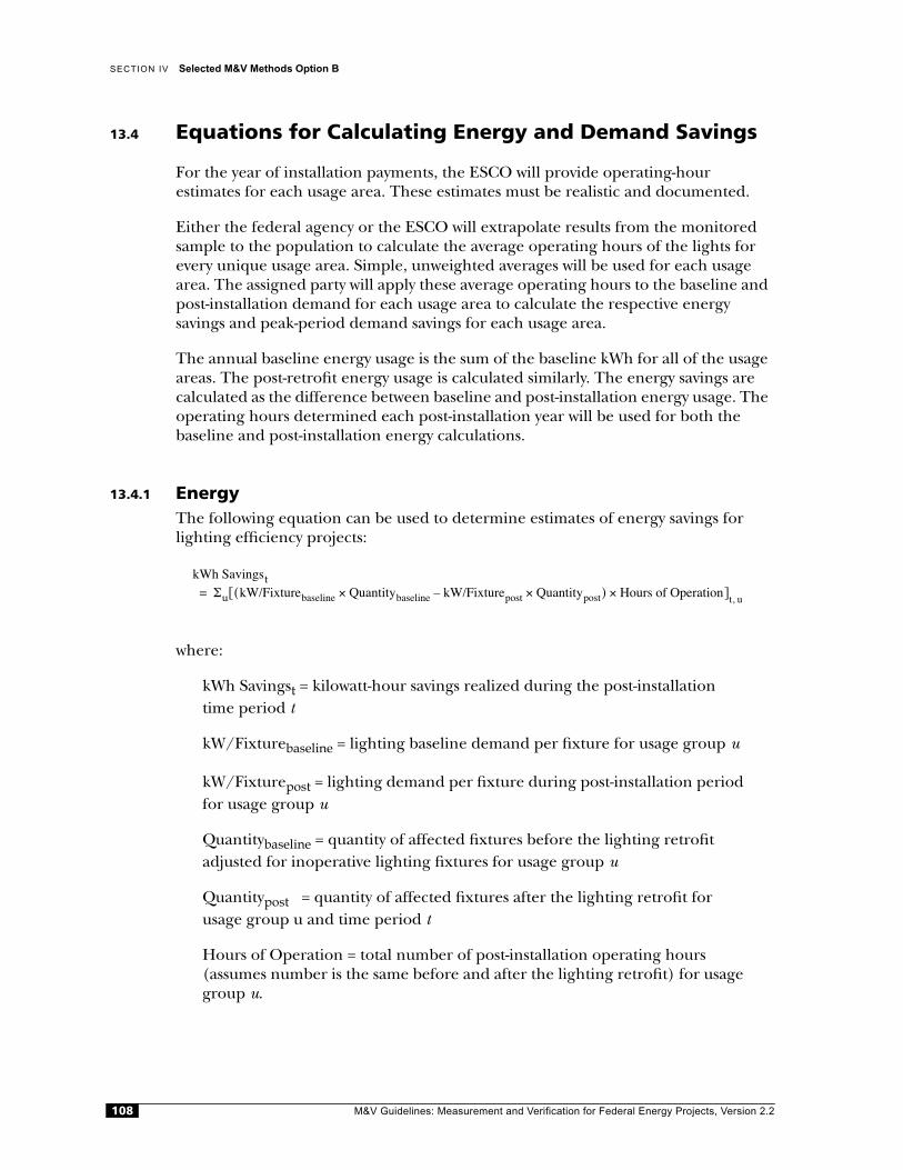
SECTION IV Selected M&V Methods Option B
13.4 Equations for Calculating Energy and Demand Savings
For the year of installation payments, the ESCO will provide operating-hourestimates for each usage area. These estimates must be realistic and documented.
Either the federal agency or the ESCO will extrapolate results from the monitored sample to the population to calculate the average operating hours of the lights for every unique usage area. Simple, unweighted averages will be used for each usage area. The assigned party will apply these average operating hours to the baseline and post-installation demand for each usage area to calculate the respective energysavings and peak-period demand savings for each usage area.
The annual baseline energy usage is the sum of the baseline kWh for all of the usage areas. The post-retrofit energy usage is calculated similarly. The energy savings are calculated as the difference between baseline and post-installation energy usage. The operating hours determined each post-installation year will be used for both the baseline and post-installation energy calculations.
13.4.1 EnergyThe following equation can be used to determine estimates of energy savings for lighting efficiency projects:
where:
kWh Savingst = kilowatt-hour savings realized during the post-installation time period t
kW/Fixturebaseline = lighting baseline demand per fixture for usage group u
kW/Fixturepost = lighting demand per fixture during post-installation period for usage group u
Quantitybaseline = quantity of affected fixtures before the lighting retrofit adjusted for inoperative lighting fixtures for usage group u
Quantitypost = quantity of affected fixtures after the lighting retrofit for usage group u and time period t
Hours of Operation = total number of post-installation operating hours (assumes number is the same before and after the lighting retrofit) for usage group u.
kWh SavingstΣu kW/Fixturebaseline Quantitybaseline kW/Fixturepost Quantitypost×–×( ) Hours of Operation×[ ]
t, u=
M&V Guidelines: Measurement and Verification for Federal Energy Projects, Version 2.2108
CHAPTER 13 Lighting Efficiency: Monitoring of Operating Hours
13.4.2 Demand Demand savings can be calculated as either an average reduction in demand or as a maximum reduction in demand.
Average reduction in demand is generally easier to calculate and is defined as kWh savings during the time period in question (e.g., utility summer peak period) divided by the hours in the time period.
Maximum demand reduction, with respect to cost savings, is typically the reduction in utility meter maximum demand under terms and conditions specified by theservicing utility. For peak load reduction, for example, the maximum demandreduction may be defined as the maximum kW reduction averaged over 30-minute intervals during the utility's summer peak period. The maximum demand reduction is usually calculated to determine savings in utility peak demand charges. Thus, if utility demand savings are to be determined, each site must define (a) how the reduction will affect the utility bill and (b) how the demand reduction will becalculated for purposes of payments to ESCOs.
13.4.3 Interactive EffectsLighting efficiency projects may have the added advantage of saving more electricity by reducing loads associated with space-conditioning systems. However, thereduction in lighting load may also increase space-heating requirements. Three options exist for estimating savings or losses associated with the interactive effects of lighting efficiency projects:
• Ignore interactive effects
• Use agreed-to, “default” interactive values such as a 5% add-on to lighting kWh savings to account for additional air-conditioning saving
• Calculate interactive effects on a site-specific basis.
13.5 Pre- and Post-Installation Submittals
For each site, the ESCO submits a project pre-installation report that includes:
• A project description and schedule
• A pre-installation equipment survey
• Estimates of energy savings
• Documentation on utility billing data
• Projected budget
• Scheduled M&V activities.
If the federal agency defines the baseline condition, the ESCO must verify anagreed-to pre-installation equipment survey.
M&V Guidelines: Measurement and Verification for Federal Energy Projects, Version 2.2 109

SECTION IV Selected M&V Methods Option B
The ESCO submits a project post-installation report following project completion and defines projected energy savings for the first year. In addition, the report includes most of the components in the project pre-installation report, addinginformation on actual rather than expected ECM installations.
13.6 Site-Specific Measurement and Verification PlanThe site-specific M&V approach may be pre-specified in the ESPC contract between the federal agency and the ESCO and/or agreed to after the award of the project. In either case, before the federal agency approves the project construction, the ESCO must submit a final M&V plan that addresses the site-specific nature of the following elements:
• Overview of approach
• Specification of savings calculations
• Identification of corresponding variables and specification of assumptions
• Identification of data sources and/or collection techniques
• Specification of data collection (i.e., sampling, site inspection, and monitoring plan), if required
• Identification and resolution of any other M&V issues.
Specific M&V issues related to lighting efficiency projects that must be addressed include the following:
• Establishment of baseline fixture wattages at current efficiency standards
• Designation of usage groups and lighting operating hours sampling plans, including accounting for lost data and unique situations at the site that can affect measurements, e.g., double-switched lighting fixtures
• Assessment of non-operating fixtures
• Methods to account for changes to baseline and post-installation fixture counts and types due to remodels
• Identification of approach for determining interactive savings.
In addition, project pre- and post-installation reports should identify the specific steps required to implement the M&V plan.
M&V Guidelines: Measurement and Verification for Federal Energy Projects, Version 2.2110
14Methods:
LE-B-02
Lighting Efficiency: Metering of Lighting Circuits
14.1 Project Definition
The lighting projects covered by this verification plan are as follows:
• Retrofits of existing fixtures, lamps and/or ballasts with an identical number of more energy-efficient fixtures, lamps and/or ballasts
• De-lamping with or without the use of reflectors.
Lighting efficiency projects reduce demand; however, the fixtures have the samepre- and post-retrofit operating hours.
14.2 Overview of Verification Method
This M&V method involves measuring all, or a representative number of, lightingcircuits to determine either or both of the following:
• Baseline and post-installation electrical energy consumption (kWh) in order to determine energy savings and average demand savings
• Baseline and post-installation electrical demand (kW) profiles in order todetermine demand savings.
Circuit measurements may be made of current flow (amperage) or power draw(wattage) per unit of time. The post-installation metering time period may becontinuous or for a reasonable, limited period of time during each contract year.
Surveys are suggested for existing (baseline) and new (post-installation) fixtures.Corrections may be required for non-operating baseline fixtures. Light levelrequirements may be specified for projects that involve reducing lighting levels.
This chapter addresses one of two M&V methods under Option B for lighting efficiency projects. Method LE-B-01 requires pre- and post-installation equipment surveys incombination with post-installation monitoring of hours of operation for establishing savings. Method LE-B-02 involves baseline and post-installation lighting circuitmeasurements for determining both demand and energy savings.
M&V Guidelines: Measurement and Verification for Federal Energy Projects, Version 2.2 111
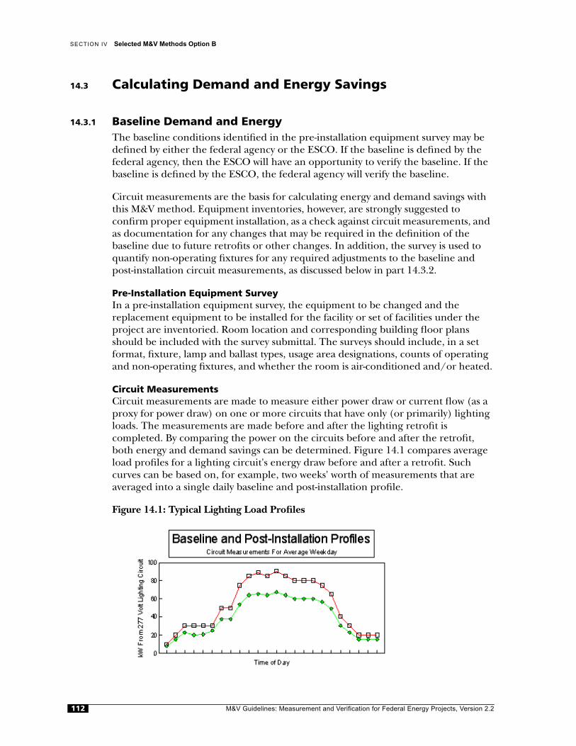
SECTION IV Selected M&V Methods Option B
14.3 Calculating Demand and Energy Savings
14.3.1 Baseline Demand and EnergyThe baseline conditions identified in the pre-installation equipment survey may be defined by either the federal agency or the ESCO. If the baseline is defined by the federal agency, then the ESCO will have an opportunity to verify the baseline. If the baseline is defined by the ESCO, the federal agency will verify the baseline.
Circuit measurements are the basis for calculating energy and demand savings with this M&V method. Equipment inventories, however, are strongly suggested toconfirm proper equipment installation, as a check against circuit measurements, and as documentation for any changes that may be required in the definition of thebaseline due to future retrofits or other changes. In addition, the survey is used to quantify non-operating fixtures for any required adjustments to the baseline and post-installation circuit measurements, as discussed below in part 14.3.2.
Pre-Installation Equipment SurveyIn a pre-installation equipment survey, the equipment to be changed and the replacement equipment to be installed for the facility or set of facilities under the project are inventoried. Room location and corresponding building floor plans should be included with the survey submittal. The surveys should include, in a set format, fixture, lamp and ballast types, usage area designations, counts of operating and non-operating fixtures, and whether the room is air-conditioned and/or heated.
Circuit MeasurementsCircuit measurements are made to measure either power draw or current flow (as a proxy for power draw) on one or more circuits that have only (or primarily) lighting loads. The measurements are made before and after the lighting retrofit iscompleted. By comparing the power on the circuits before and after the retrofit, both energy and demand savings can be determined. Figure 14.1 compares average load profiles for a lighting circuit's energy draw before and after a retrofit. Such curves can be based on, for example, two weeks' worth of measurements that are averaged into a single daily baseline and post-installation profile.
Figure 14.1: Typical Lighting Load Profiles
M&V Guidelines: Measurement and Verification for Federal Energy Projects, Version 2.2112

CHAPTER 14 Lighting Efficiency: Metering of Lighting Circuits
The circuits must be carefully selected to ensure the following:
• Only lighting loads that are affected by the retrofit are on the measured circuit(s) (typically, 277-V circuits are used).
• If other loads are on the circuit(s), the non-lighting loads should be minimal, and well defined, and they should not vary from before the retrofit to after it is complete.
If only a subset of affected lighting circuits are metered, the following issues must be addressed:
• Which lighting loads are on each lighting circuit?
• Which lighting circuits are representative of the entire facility, certain areas, or certain lighting usage groups?
• What are the appropriate lighting circuit sample sizes?
Whether all the circuits or just a sample of them are metered, it is important tospecify how long the metering will be conducted in order to determine arepresentative baseline and post-installation operating profile.
For each facility, the ESCO or federal agency will develop a sampling plan formonitoring circuits. The sampling plan may concentrate measurements in areas with the greatest savings.
MetersThe ESCO will specify the meter to be used in the site-specific M&V plan.Measurements of circuits are typically made with either of the following:
• Current transducers connected to one or more legs of a lighting circuit. Current data measurements are taken over an extended period of time. Voltage and power factor data are taken as spot measurements and then assumed to beconstant during the time period of the current metering. True RMS readingsare preferred.
• True RMS current and potential (voltage) transducers used to measure power continuously during the time period of circuit monitoring. This type of metering can be more accurate than just current measurement, but it is also moreexpensive.
The meter and recording device may be required to measure and record data for all utility time-of-use costing periods. The ESCO should use a data logger that records status at frequent intervals (e.g., at least every 15 minutes). “Raw” as well as “compiled” data from the meter(s) must be made available to the federal agency.
Period of MonitoringMetering provides an estimate of demand profiles and annual energy use. Theduration and timing of the installation of circuit monitors have a strong influence on the accuracy of energy savings estimates. Metering should not be installed during
M&V Guidelines: Measurement and Verification for Federal Energy Projects, Version 2.2 113
SECTION IV Selected M&V Methods Option B
significant holiday or vacation periods. If a holiday or vacation falls within themetering installation period, the metering period should be extended as many days as the holiday or vacation lasted.
If less than continuous metering is used, the energy use and demand profiles obtained during the metered period will be extrapolated to the full year. A minimum metering period of three weeks is recommended for almost all situations. Forsituations in which lighting might vary seasonally, such as classrooms, or according to a scheduled activity, it may be necessary to determine lighting energy use andprofiles during different times of the year.
The ESCO-supplied site-specific M&V plan will include a detailed, agreed-to sample plan and metering plan.
14.3.2 Adjustments to Baseline DemandBefore new lighting fixtures are installed, adjustments to the baseline demandmay be required for non-operating fixtures. In addition, after ECM installation,adjustments to baseline demand may be required because of remodeling orchanges in occupancy. Methods for making adjustments should be specified in thesite-specific M&V plan.
The party responsible for defining the baseline will also identify any non-operating fixtures. Non-operating fixtures are those that are typically operating but have broken lamps, ballasts, and/or switches that are intended for repair.
A de-lamped fixture is not a non-operating fixture; thus, de-lamped fixtures should have their own unique wattage designations. Fixtures that have been disabled orde-lamped or that are broken and not intended for repair should not be included in the calculation of baseline demand or energy. They should, however, be noted in the lighting survey to avoid confusion.
For non-operating fixtures, the baseline demand may be adjusted by using values from the standard table of fixture wattages or from fixture wattage measurements. The adjustment for inoperative fixtures will be limited to some percentage of the total fixture count per facility, e.g., 10%. If, for example, more than 10% of the total number offixtures are inoperative, the number of fixtures beyond 10% will be assumed to have a baseline fixture wattage of zero.
14.3.3 Post-Installation DemandThe post-installation conditions should be identified in the post-installationequipment survey, which is typically prepared by the ESCO and verified by thefederal agency. The circuit measurements are then used to define post-installation demand and energy, as discussed above.
M&V Guidelines: Measurement and Verification for Federal Energy Projects, Version 2.2114
CHAPTER 14 Lighting Efficiency: Metering of Lighting Circuits
14.4 Equations for Calculating Energy and Demand Savings
For the year of installation payments, the ESCO will provide energy and demandsavings estimates. These estimates must be realistic and documented. Either thefederal agency or the ESCO will extrapolate results from the metering data todetermine demand and energy savings.
14.4.1 EnergyTo determine estimates of energy savings for lighting efficiency projects, use the following equation:
where:
kWh Savings t = the kilowatt-hour savings realized during the time period t, where t can be a whole year, a week, weekdays, weekends, or a particular hour of the day
(Average kWhbaseline)t = the lighting baseline energy use averaged for all the time period t measurements
(Average kWhpost)t = the lighting post-installation energy use averaged for all the time period t measurements.
Implicit in this equation is the assumption that baseline and post-installation lighting operating hours are the same.
14.4.2 Demand Demand savings can be calculated as either an average reduction in demand or as a maximum reduction in demand.
Average reduction in demand is generally easier to calculate. It is defined as kWhsavings during the time period in question (e.g., utility summer peak period) divided by the hours in the time period.
Maximum demand reduction with respect to cost savings, is typically the reductionin utility meter maximum demand under terms and conditions specified by theservicing utility. For peak-load reduction, for example, the maximum demandreduction may be defined as the maximum kW reduction averaged over 30-minute intervals during the utility's summer peak period. The maximum demand reduction is usually calculated to determine savings in utility peak demand charges. Thus, if utility demand savings are to be determined, each site must define (a) how the reduction will affect the utility bill, and (b) how the demand reduction will becalculated for purposes of payments to ESCOs.
kWh Savingst Average kWhbaseline( )t
Average kWhpost( )t
–=
M&V Guidelines: Measurement and Verification for Federal Energy Projects, Version 2.2 115
SECTION IV Selected M&V Methods Option B
14.4.3 Interactive EffectsLighting efficiency projects may have the added advantage of saving more electricity by reducing loads associated with space-conditioning systems; however, the reduction in lighting load may also increase space heating requirements. Three options exist for estimating savings or losses associated with the interactive effects of lightingefficiency projects:
• Ignore interactive effects.
• Use agreed-to, “default” interactive values such as a 5% add on to lighting kWh savings to account for additional air-conditioning saving.
• Calculate interactive affects on a site-specific basis.
14.5 Pre- and Post-Installation Submittals
For each site, the ESCO submits a project pre-installation report that includes the following:
• A project description and schedule
• A pre-installation equipment survey
• Estimates of energy savings
• Documentation on utility billing data
• Projected budget
• Scheduled M&V activities.
If the federal agency defines the baseline condition, the ESCO must verify aagreed-to pre-installation equipment survey.
The ESCO submits a project post-installation report following project completion and defines projected energy savings for the first year. In addition, the report includes many of the components in the project pre-installation report, addinginformation on actual rather than expected ECM installations.
14.6 Site-Specific Measurement and Verification Plan
The site-specific M&V approach may be pre-specified in the ESPC between thefederal agency and the ESCO and/or agreed to after the award of the project. In either case, before the federal agency approves project construction, the ESCO must submit a final M&V plan that addresses the following elements on a site-specific basis:
• Overview of approach
• Specification of savings calculations
M&V Guidelines: Measurement and Verification for Federal Energy Projects, Version 2.2116

CHAPTER 14 Lighting Efficiency: Metering of Lighting Circuits
• Identification of corresponding variables and specification of assumptions
• Identification of data sources and/or collection techniques
• Specification of data collection (i.e., sampling, site inspection, and monitoring plan), if required
• Identification and resolution of any other M&V issues.
Specific M&V issues related to lighting efficiency projects that need to be addressed include the following:
• Establishment of baseline fixture wattages at current efficiency standards
• Selection of lighting circuits to be metered
• Selection of metering equipment
• Selection of time period for metering
• Assessment of non-operating fixtures
• Methods to account for changes to baseline and post-installation fixture counts and types due to remodels
• Identification of approach for determining interactive savings.
In addition, project pre- and post-installation reports should identify the specific steps required to implement the M&V plan.
M&V Guidelines: Measurement and Verification for Federal Energy Projects, Version 2.2 117
15Methods:
LC-B-01
Lighting Controls: Monitoring of Operating Hours
15.1 Project Definition
The lighting projects covered by this M&V plan are installation of occupancy sensors or daylighting controls with or without changes to fixtures, lamps, or ballasts.
These lighting control projects reduce fixture operating hours.
15.2 Overview of Verification Method
This method is similar to Option A methods LC-A-01 and LC-A-02, in that surveys will be made of all baseline and post-installation lighting fixtures and controls andfixture wattages will be measured on a standard table of measurements. Thedifference is that, instead of stipulating operating hours, the operating hours are measured throughout the term of the agreement either at regular intervals orcontinuously.
Surveys are required of existing (baseline) and new (post-installation) fixtures and controls. Corrections may be required for non-operating fixtures. Light level requirements may be specified for projects that involve reducing lighting levels.
Fixture wattages will be determined from any of the following:
• Measurements of representative fixtures or lighting circuits
• Documentation on each fixture or ballast or lamp combination
• A table of standard wattages.
Post-installation hours of operation will be determined by monitoring a statistically valid sample of fixtures and rooms. The monitoring time period must be reasonable and account for any seasonal variations.
This chapter addresses one of two M&V methods under Option B for lighting con-trol projects. Method LC-B-01 requires pre- and post-installation equipment surveys in combination with pre- and post-installation metering of hours of operation to establish savings. Chapter 16 addresses method LC-B-02, which involves baseline and post-installation lighting circuit measurements for determining both demand and energy savings.
M&V Guidelines: Measurement and Verification for Federal Energy Projects, Version 2.2118
CHAPTER 15 Lighting Controls: Monitoring of Operating Hours
15.3 Calculating Demand and Energy Savings
15.3.1 Baseline DemandThe baseline conditions identified in the pre-installation equipment survey may be defined by either the federal agency or the ESCO. If the baseline is defined by the federal agency, the ESCO will have an opportunity to verify the baseline. If thebaseline is defined by the ESCO, the federal agency will verify the baseline.
In the pre-installation equipment survey, the equipment to be changed and the replacement equipment to be installed (if an efficiency retrofit is to be doneconcurrently) are inventoried. Room locations and corresponding building floor plans should be included with the survey submittal. The surveys will include, in a set format, fixture, lamp, and ballast types; lighting controls; usage area designations; counts of operating and non-operating fixtures; and whether the room isair-conditioned and/or heated.
Fixture wattages will be based on a table of standard fixture wattages or spot/short-term metering.
Wattage TableFixture wattages will be determined from a standard table unless otherdocumentation is provided. A standard table of fixture wattages should containcommon lamp and ballast combinations. If a fixture is not in the table, the partyconducting the pre-installation equipment survey should either (a) take wattage measurements for a representative sample of fixtures, or (b) provide a documented source of the fixture wattages for approval by the other party.
In general, a standard table of fixture wattages should be used for the baselinefixtures, and documented manufacturers' data should be used for post-installation fixtures.
Fixture Wattage MeteringFixture wattages will be measured. An example of a metering protocol is as follows:
The ESCO will take 15-minute, true RMS wattage measurements from at least six fixtures representative of the baseline and post-installation fixtures (actual values may vary by application). Readings will be averaged to determineper-fixture wattage values. For post-installation fixtures, readings should be taken only after the new fixtures have been operating for at least 100 hours. Meters used for this task will be calibrated and have an accuracy of ±2% of reading, or better.
15.3.2 Adjustments to Baseline DemandBefore new lighting fixtures are installed, adjustments to the baseline demandmay be required for non-operating fixtures. In addition, after ECM installation,adjustments to baseline demand may be required because of remodeling orchanges in occupancy.
M&V Guidelines: Measurement and Verification for Federal Energy Projects, Version 2.2 119

SECTION IV Selected M&V Methods Option B
Methods for making adjustments should be specified in the site-specific M&V plan.
The party responsible for defining the baseline will also identify any non-operating fixtures. Non-operating fixtures are those that are typically operating but that havebroken lamps, ballasts, and/or switches that are intended for repair.
A de-lamped fixture is not a non-operating fixture; thus, de-lamped fixtures should have their own unique wattage designations. Fixtures that have been disabled orde-lamped or that are broken and not intended for repair should not be included in the calculation of baseline demand or energy. They should, however, be noted in the lighting survey to avoid confusion.
For non-operating fixtures, the baseline demand may be adjusted by using values from the standard table of fixture wattages or from fixture wattage measurements. The adjustment for inoperative fixtures will be limited to a percentage of the total fixture count per facility, e.g., 10%. If, for example, more than 10% of the total number of fixtures are inoperative, the number of fixtures beyond 10% will be assumed to have abaseline fixture wattage of zero.
15.3.3 Post-Installation DemandThe post-installation conditions identified in the post-installation equipment survey will be defined by the ESCO and verified by the federal agency. The techniquesdiscussed in part 15.3.1 can be used to inventory the installed equipment.
15.3.4 Operating HoursTo determine how operating hours will be measured (both before and after thecontrol devices are installed), three key issues must be defined:
• The appropriate usage groups and sample sizes for metering each facility or group of similar facilities
• Whether lighting circuit measurements or lighting loggers will be used
• How long the operating hours should be metered to determine a representative operating profile.
Usage GroupsBuilding usage areas will be identified for those areas with comparable averageoperating hours, as determined by the lights operating during the year or by each of the electric utility's costing periods. Usage areas must be defined in a way that groups together areas that have similar occupancies and lighting operating hour schedules.
For each unique usage area, the ESCO or federal agency will develop a sampling plan to monitor the average operating hours of either a sample of fixtures or asample of circuits. Sampling guidelines are provided in Appendix D.
M&V Guidelines: Measurement and Verification for Federal Energy Projects, Version 2.2120

CHAPTER 15 Lighting Controls: Monitoring of Operating Hours
MetersThe ESCO will specify the meter to be used in the site-specific M&V plan. Operating hours are typically measured with either of the following:
• “Light loggers,” which are devices that measure the operating hours of individual fixtures through the use of photocells. A wide variety of products are available that store information that can be translated into either elapsed run times forfixtures (run-time loggers) or actual load profiles of on and off times for fixtures (time-of-use loggers).
• Current or power measurements of lighting circuits, which, when calibrated to the total connected lighting load on the circuit, can be used to determine how many fixtures were operating in terms of elapsed time over a period of time or actual time-of-use load profiles.
The meter and recording device may be required to measure and record data for all utility time-of-use costing periods. The ESCO must use a data logger that recordsstatus at frequent intervals (e.g., at least every 15 minutes). “Raw” as well as compiled” data from the meter(s) must be made available to the federal agency.
If the ESCO chooses to monitor circuits to determine average operating hours, the ESCO will use run-time or power recording meters that record the circuit on/off pattern in each utility costing period. The ESCO will not monitor circuits when the circuit serving the lighting retrofit load also serves other non-lighting loads thatcannot be distinguished from the lighting load. Thus, only when lighting andnon-lighting loads are separable, may circuits be monitored.
Period of MonitoringMonitoring provides an estimate of annual equipment operating hours. Theduration and timing of the installation of run-time monitoring have a stronginfluence on the accuracy of operating hours estimates. Run-time monitoring should not be installed during significant holiday or vacation periods. If a holiday orvacation falls within the run-time monitoring installation period, the duration of monitoring should be extended for as many days as the holiday or vacation lasted.
If less than continuous monitoring is used, the lighting operating hours during the monitored period will be extrapolated to the full year. A minimum monitoring period of three weeks is recommended for almost all usage area groups. For situations in which lighting might vary seasonally, such as classrooms, or according to ascheduled activity, it may be necessary to determine lighting operation hoursduring different times of the year.
The ESCO supplied site-specific M&V plan will include the detailed, agreed-to sample plan and monitoring plan.
M&V Guidelines: Measurement and Verification for Federal Energy Projects, Version 2.2 121
SECTION IV Selected M&V Methods Option B
15.4 Equations for Calculating Energy and Demand Savings
For the year of installation payments, the ESCO will provide operating-hourestimates for each usage area. These estimates must be realistic and documented.
Either the federal agency or the ESCO will extrapolate results from the monitored sample to the population to calculate the average operating hours of the lights for every unique usage area. Simple, unweighted averages will be used for each usage area. To calculate the respective energy savings and peak period demand savings for each usage area, the assigned party will apply these average operating hours to the baseline and post-installation demand for each usage area.
The annual baseline energy usage is the sum of the baseline kWh for all of the usage areas. The post-retrofit energy usage is calculated similarly. The energy savings are calculated as the difference between baseline and post-installation energy usage. The operating hours determined each post-installation year will be used for both the baseline and post-installation energy calculations.
To avoid double-counting the savings from energy-efficiency projects that also have lighting control projects applied, the ESCO will meter the pre-installation and post-installation controlled hours of operation as the basis for calculating lightingefficiency savings. See below for calculations.
15.4.1 EnergyTo avoid double-counting lighting efficiency and control projects' savings, thesavings equations for both types of projects are combined into a single equation:
where:
kWh Savingst = kilowatt-hour savings realized during the post-installation time period t
kW/Fixturebaseline = lighting baseline demand per fixture
kW/Fixturepost = lighting demand per fixture during post-installation period for usage group u
Quantitybaseline = the quantity of affected fixtures before the lighting retrofit adjusted for inoperative and non-operative lighting fixtures for usage group u
Quantitypost = quantity of affected fixtures after the lighting retrofit for usage group u
kWh Savingst Σu kW/Fixture Quantity Hours of Operation××( )baseline[=
- kWh/Fixture Quantity Hours of Operation××( )post ]t, u
M&V Guidelines: Measurement and Verification for Federal Energy Projects, Version 2.2122
CHAPTER 15 Lighting Controls: Monitoring of Operating Hours
Hours of Operationbaseline = total number of operating hours during thepre-installation period for usage group u
Hours of Operationpost = total number of operating hours during thepost-installation period for usage group u.
This equation is based on the following:
• Savings for energy efficiency lighting projects as defined in the followingequation:
• Savings for lighting control projects as defined in the following equation:
15.4.2 Demand Demand savings can be calculated as either an average reduction in demand or as a maximum reduction in demand.
Average reduction in demand is generally easier to calculate. It is defined as kWhsavings during the time period in question (e.g., utility summer peak period) divided by the hours in the time period.
Maximum demand reduction with respect to cost savings is typically the reduction in utility meter maximum demand under terms and conditions specified by theservicing utility. For peak-load reduction, for example, the maximum demandreduction may be defined as the maximum kW reduction averaged over 30-minute intervals during the utility's summer peak period. The maximum demand reduction is usually calculated to determine savings in utility peak demand charges. Thus, if utility demand savings are to be determined, each site must define (a) how the reduction will affect the utility bill, and (b) how the demand reduction will becalculated for purposes of payments to ESCOs.
15.5 Interactive Effects
Lighting efficiency projects may have the added advantage of saving more electricity by reducing loads associated with space-conditioning systems; however, the reduction in lighting load may also increase space-heating requirements. Three options exist for estimating savings or losses associated with the interactive effects of lightingefficiency projects:
kWh Savings Σu kW/Fixture Quantity×( )baseline
kW/Fixture Quantity )post× ] Hours of Operation×post
)t, u
(–
[(=
kWh Savings ΣuHours of Operation( baseline Hours of Operationpost )–[ kW/Fixture(× Quantity×
baseline) ]
t, u
=
M&V Guidelines: Measurement and Verification for Federal Energy Projects, Version 2.2 123
SECTION IV Selected M&V Methods Option B
• Ignore interactive effects
• Use agreed-to, “default” interactive values such as a 5% adder to lighting kWhsavings to account for additional air-conditioning saving
• Calculate interactive affects on a site-specific basis.
15.6 Pre- and Post-Installation Submittals
For each site, the ESCO submits a project pre-installation report that includes the following:
• A project description and schedule
• A pre-installation equipment survey
• Estimates of energy savings
• Documentation on utility billing data
• Projected budget
• Scheduled M&V activities.
If the federal agency defines the baseline condition, the ESCO must verify anagreed-to pre-installation equipment survey.
The ESCO submits a project post-installation report following project completion and defines projected energy savings for the first year. The report includes many of the components in the project pre-installation report, adding information on actual rather than expected ECM installations.
15.7 Site-Specific Measurement and Verification Plan
The site-specific M&V approach may be pre-specified in the ESPC between thefederal agency and the ESCO and/or agreed to after the award of the project. In either case, before the federal agency's approval of project construction, the ESCO will need to submit a final M&V plan that addresses the following elements on asite-specific basis:
• Overview of approach
• Specification of savings calculations
• Identification of corresponding variables and specification of assumptions
• Identification of data sources and/or collection techniques
• Specification of data collection (i.e., sampling site inspection, and monitoring plan), if required
• Identification and resolution of any other M&V issues.
M&V Guidelines: Measurement and Verification for Federal Energy Projects, Version 2.2124

CHAPTER 15 Lighting Controls: Monitoring of Operating Hours
Specific M&V issues that must be addressed related to lighting efficiency projects include the following:
• Decision whether to establish baseline fixture wattages at current efficiencystandards
• Avoiding double-counting the savings from energy-efficiency projects that are controlled
• Designation of usage groups and lighting operating hours sampling plans, including accounting for lost data and unique situations at the site that can affect measurements; e.g., double-switched lighting fixtures
• Assessment of non-operating fixtures
• Methods to account for changes to baseline and post-installation fixture counts and types due to remodels, and identification of approach for determininginteractive savings.
M&V Guidelines: Measurement and Verification for Federal Energy Projects, Version 2.2 125
16Methods:
LC-B-02
Lighting Controls: Metering of Lighting Circuits
16.1 Project Definition
The lighting projects covered by this verification plan are installations of occupancy sensors or daylighting controls with or without changes to fixtures, lamps, or ballasts.
These lighting controls projects reduce fixture operating hours.
16.2 Overview of Verification Method
This M&V method involves measuring all, or a representative number of, lighting circuits to determine either or both of the following:
• Baseline and post-installation electrical energy consumption (kWh) in order to determine energy savings and average demand savings
• Baseline and post-installation electrical demand (kW) profiles in order todetermine demand savings.
Circuit measurements may be made of current flow (amperage) or power draw (wattage) per unit of time. The post-installation metering time period may becontinuous or for a reasonable, limited period of time during each contract year.
Surveys are suggested for existing (baseline) and new (post-installation) fixtures. Corrections may be required for non-operating baseline fixtures. Light levelrequirements may be specified for projects that involve reducing lighting levels.
This chapter addresses one of two M&V methods under Option B for lightingcontrols projects. Method LC-B-02 involves baseline and post-installation lightingcircuit measurements to determine both demand and energy savings. The previous chapter address method LC-B-01, which requires pre- and post-installationequipment surveys in combination with baseline and post-installation monitoringof hours of operation for establishing savings.
M&V Guidelines: Measurement and Verification for Federal Energy Projects, Version 2.2126
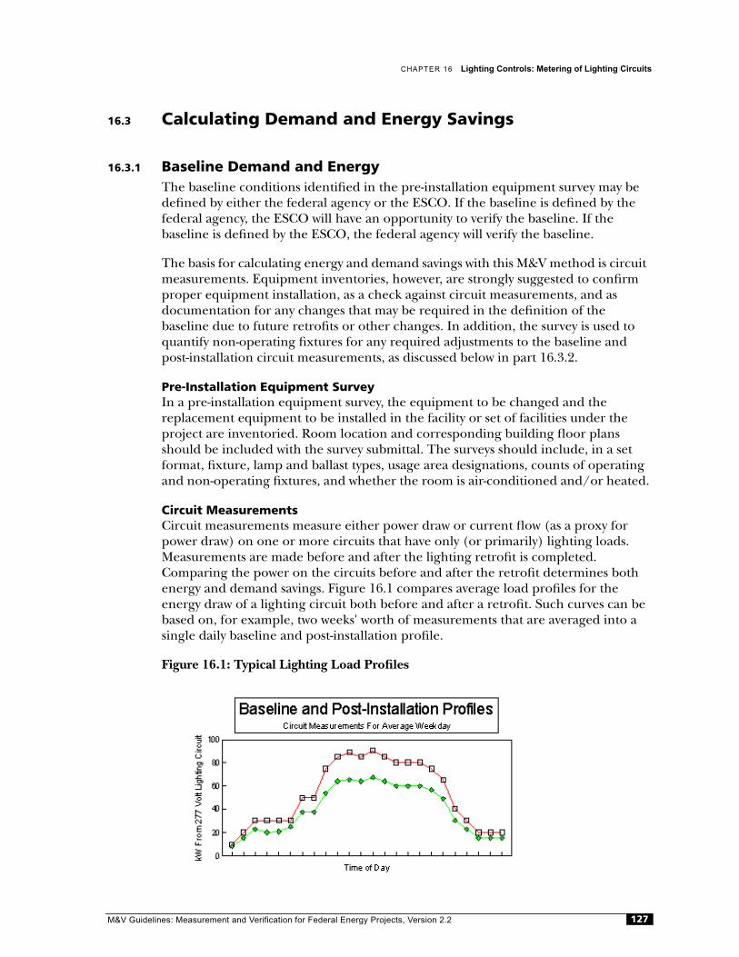
CHAPTER 16 Lighting Controls: Metering of Lighting Circuits
16.3 Calculating Demand and Energy Savings
16.3.1 Baseline Demand and EnergyThe baseline conditions identified in the pre-installation equipment survey may be defined by either the federal agency or the ESCO. If the baseline is defined by the federal agency, the ESCO will have an opportunity to verify the baseline. If thebaseline is defined by the ESCO, the federal agency will verify the baseline.
The basis for calculating energy and demand savings with this M&V method is circuit measurements. Equipment inventories, however, are strongly suggested to confirm proper equipment installation, as a check against circuit measurements, and asdocumentation for any changes that may be required in the definition of thebaseline due to future retrofits or other changes. In addition, the survey is used to quantify non-operating fixtures for any required adjustments to the baseline and post-installation circuit measurements, as discussed below in part 16.3.2.
Pre-Installation Equipment SurveyIn a pre-installation equipment survey, the equipment to be changed and the replacement equipment to be installed in the facility or set of facilities under the project are inventoried. Room location and corresponding building floor plans should be included with the survey submittal. The surveys should include, in a set format, fixture, lamp and ballast types, usage area designations, counts of operating and non-operating fixtures, and whether the room is air-conditioned and/or heated.
Circuit MeasurementsCircuit measurements measure either power draw or current flow (as a proxy for power draw) on one or more circuits that have only (or primarily) lighting loads. Measurements are made before and after the lighting retrofit is completed.Comparing the power on the circuits before and after the retrofit determines both energy and demand savings. Figure 16.1 compares average load profiles for the energy draw of a lighting circuit both before and after a retrofit. Such curves can be based on, for example, two weeks' worth of measurements that are averaged into a single daily baseline and post-installation profile.
Figure 16.1: Typical Lighting Load Profiles
M&V Guidelines: Measurement and Verification for Federal Energy Projects, Version 2.2 127

SECTION IV Selected M&V Methods Option B
The circuits must be carefully selected to ensure either of the following:
• Only lighting loads that are affected by the retrofit are on the measurementcircuit(s) (typically 277-V circuits are used).
• If other loads are on the circuit(s), the non-lighting loads should be minimal, well defined, and not vary from before the retrofit is complete to after it iscomplete.
If only a subset of affected lighting circuits is metered, the following issues must be addressed:
• Which lighting loads are on each lighting circuit?
• Which lighting circuits are representative of the entire facility, certain areas, or certain lighting usage groups?
• What are the appropriate lighting circuit sample sizes?
Whether all or just a sample of circuits are metered, it is important to specify how long the metering will be conducted in order to determine a representative baseline and post-installation operating profile.
For each facility, the ESCO or federal agency will develop a sampling plan formonitoring circuits. The sampling plan may concentrate measurements in areas with the greatest savings.
MetersThe ESCO will specify the meter to be used in the site-specific M&V plan. Circuits are typically measured with either of the following:
• Current transducers connected to one or more legs of a lighting circuit. Current data measurements are taken over an extended period of time. Voltage and power factor data are taken as spot measurements and then assumed to beconstant during the time period of the current metering. True RMS readingsare preferred.
• True RMS current and potential (voltage) transducers are used to measure power continuously during the time period of circuit monitoring. This type of metering can be more accurate than just current measurement, but it is also moreexpensive.
The meter and recording device may be required to measure and record data for all utility time-of-use costing periods. The ESCO should use a data logger that records status at frequent intervals (e.g., at least every 15 minutes). “Raw” as well as “com-piled” data from the meter(s) must be made available to the federal agency.
Period of MeteringMetering is intended to provide an estimate of demand profiles and annual energy use. The duration and timing of the installation of circuit metering have a strong
M&V Guidelines: Measurement and Verification for Federal Energy Projects, Version 2.2128
CHAPTER 16 Lighting Controls: Metering of Lighting Circuits
influence on the accuracy of energy savings estimates. Metering should not be installed during significant holiday or vacation periods. If a holiday or vacation falls within the metering installation period, the duration of metering should be extended for as many days as the holiday lasted.
If less than continuous metering is used, the energy use and demand profiles obtained during the monitored period will be extrapolated to the full year. Aminimum metering period of three weeks is recommended for almost all situations. For situations in which lighting might vary seasonally, such as in classrooms, or according to a scheduled activity, it may be necessary to determine lighting energy use and profiles during different times of the year.
The ESCO-supplied site-specific M&V plan will include a detailed, agreed-to sample plan and metering plan.
16.3.2 Adjustments to Baseline DemandBefore the new lighting fixtures are installed, adjustments to the baseline demand may be required for non-operating fixtures. After the ECM installation, adjustments to baseline demand may be required because of remodeling or changes inoccupancy. Methods for making adjustments should be specified in the site-specific M&V plan.
The party responsible for defining the baseline will also identify any non-operating fixtures. Non-operating fixtures are those that are typically operating but that havebroken lamps, ballasts, and/or switches that are intended for repair.
A de-lamped fixture is not a non-operating fixture; thus, de-lamped fixtures should have their own unique wattage designations. Fixtures that have been disabled orde-lamped or that are broken and not intended for repair should not be included in the calculation of baseline demand or energy. They should, however, be noted in the lighting survey to avoid confusion.
For non-operating fixtures, the baseline demand may be adjusted by using values from the standard table of fixture wattages or from fixture wattage measurements. The adjustment for inoperative fixtures will be limited to a percentage of the total fixture count per facility, e.g., 10%. If, for example, more than 10% of the total number of fixtures are inoperative, the number of fixtures beyond 10% will be assumed to have abaseline fixture wattage of zero.
16.3.3 Post-Installation DemandThe post-installation conditions should be identified in the post-installationequipment survey, which is typically prepared by the ESCO and verified by thefederal agency. The circuit measurements are then used to define post-installation demand and energy, as discussed above.
M&V Guidelines: Measurement and Verification for Federal Energy Projects, Version 2.2 129

SECTION IV Selected M&V Methods Option B
16.4 Equations for Calculating Energy and Demand Savings
For the year of installation payments, the ESCO will provide energy and demandsavings estimates. These estimates must be realistic and documented.
Either the federal agency or the ESCO will extrapolate results from the metering data to determine demand and energy savings.
16.4.1 EnergyTo determine estimates of energy savings for lighting controls projects, use thefollowing equation:
where:
kWh Savingst = the kilowatt-hour savings realized during the time period t, where t can be a whole year, a week, weekdays, weekends, or a particular hour of the day
(Average kWhbaseline)t = the lighting baseline energy use averaged for all the time period t measurements
(Average kWhpost)t = the lighting post-installation energy use averaged for all the time period t measurements.
Implicit in this equation is the assumption that baseline and post-installation lighting operating hours are the same.
16.4.2 DemandDemand savings can be calculated as either an average reduction in demand or as a maximum reduction in demand.
Average reduction in demand is generally easier to calculate. It is defined as kWhsavings during the time period in question (e.g., utility summer peak period) divided by the hours in the time period.
Maximum demand reduction is the largest reduction in demand that occurs from the retrofit during a specified period of time. For peak load reduction, for example,the maximum demand reduction may be defined as the maximum kW reductionaveraged over 30-minute intervals during the utility's summer peak period. Themaximum demand reduction is usually calculated to determine savings in utility peak demand charges. Thus, if utility demand savings are to be determined, each site must define how the reduction will affect the utility bill and how the demandreduction will be calculated for purposes of payments to ESCOs.
kWh Savingst Average kWhbaseline )t Average kWhpost )t(–(=
M&V Guidelines: Measurement and Verification for Federal Energy Projects, Version 2.2130
CHAPTER 16 Lighting Controls: Metering of Lighting Circuits
16.4.3 Interactive EffectsLighting efficiency projects may have the added advantage of saving more electricity by reducing loads associated with space-conditioning systems; however, the reduction in lighting load may also increase space-heating requirements. Three options exist for estimating savings or losses associated with the interactive effects of lightingefficiency projects:
• Ignore interactive effects
• Use agreed-to, “default” interactive values such as a 5% adder to lighting kWhsavings to account for additional air conditioning savings
• Calculate interactive affects on a site-specific basis.
16.5 Pre- and Post-Installation Submittals
For each site, the ESCO submits a project pre-installation report that includes the following:
• A project description and schedule
• A pre-installation equipment survey
• Estimates of energy savings
• Documentation on utility billing data
• Projected budget
• Scheduled M&V activities.
If the federal agency defines the baseline condition, the ESCO must verify anagreed-to pre-installation equipment survey.
The ESCO submits a project post-installation report following project completion and defines projected energy savings for the first year. The report includes many of the components in the project pre-installation report, adding information on actual rather than expected ECM installations.
16.6 Site-Specific Measurement and Verification Plan
The site-specific measurement and verification approach may be pre-specified in the ESPC between the federal agency and the ESCO and/or agreed to after the awardof the project. In either case, before the federal agency approves the projectconstruction, the ESCO must submit a final M&V plan that addresses the following elements on a site-specific basis:
• Overview of approach
• Specification of savings calculations
M&V Guidelines: Measurement and Verification for Federal Energy Projects, Version 2.2 131

SECTION IV Selected M&V Methods Option B
• Identification of corresponding variables and specification of assumptions
• Identification of data sources and/or collection techniques
• Specification of data collection (i.e., sampling, site inspection, and monitoring plan), if required
• Identification and resolution of any other M&V issues.
Specific M&V issues related to lighting efficiency projects that must be addressed include the following:
• Establishment of baseline fixture wattages at current efficiency standards
• Avoiding double-counting the savings from energy-efficiency projects that are controlled
• Selection of lighting circuits to be metered
• Selection of metering equipment
• Selection of time period for metering
• Assessment of non-operating fixtures
• Methods to account for changes to baseline and post-installation fixture counts and types due to remodels
• Identification of the approach for determining interactive savings.
In addition, project pre- and post-installation reports should identify the specific steps required to implement the M&V plan.
M&V Guidelines: Measurement and Verification for Federal Energy Projects, Version 2.2132
17Methods:
CLM-B-01
Constant-Load Motor Efficiency: Metering of Operating Hours
17.1 ECM Definition
Constant-load motor efficiency projects involve the replacement of existing (baseline) motors with high-efficiency motors that serve constant-load systems. These ECMs are called constant-load motor efficiency projects because the power draw of the motors does not vary over time. These projects reduce demand and energy use.
This M&V method is appropriate only for projects in which constant-load motors are replaced with similar capacity constant-speed motors, with two exceptions:
• Baseline motors may be replaced with smaller high-efficiency motors when theoriginal motor was oversized for the load.
• Constant-speed motor drives may be adjusted to account for the difference in slip between the baseline motor and the high-efficiency motor.
If motor changes are accompanied by a change in operating schedule, a change in flow rate, or the installation of variable-speed controls, other M&V methods are moreappropriate.
17.2 Overview of Verification Method
Under Option B, method CLM-B-01 is the only specified technique for verifyingconstant-load motor efficiency projects. Surveys are required to document existing (baseline) and new (post-installation) motors. The surveys should include thefollowing (in a set format) for each motor:
• Nameplate data
• Operating schedule
• Spot and short-term metering data
• Motor application definitions
• Location.
M&V Guidelines: Measurement and Verification for Federal Energy Projects, Version 2.2 133
SECTION IV Selected M&V Methods Option B
Metering is required on at least a sample of motors to determine average powerdraw for baseline and new motors. Demand savings are based on the average kWmeasured before the new motors are installed minus the average kW measured after they are installed. Allowances may be made for differences in motor slip between existing and new motors.
Operating hours for the baseline and/or post-installation periods will be determined with short-term or long-term metering on at least a sample of the motors. Inaddition, metering can be used to (a) confirm constant loading and (b) determine average motor power draw (if normalization is required).
17.3 Calculating Demand and Energy Savings
17.3.1 Baseline DemandThe baseline conditions identified in the pre-installation equipment survey will be defined by either the federal agency or the ESCO. If the baseline is defined by the federal agency, the ESCO will have the opportunity to verify the baseline. If thebaseline is defined by the ESCO, the federal agency will verify the baseline.
Steps involved in establishing the baseline demand are as follows:
• Conduct a pre-installation equipment survey
• Perform spot metering of existing motors
• Perform short-term metering of existing motors.
The equipment survey is described in this subsection. Spot and short-term metering are discussed in part 16.5, as these types of metering activities are also requiredduring the post-installation period.
In the pre-installation equipment survey, the equipment to be changed and the replacement equipment to be installed will be inventoried. Motor location andcorresponding building floor plans should be included with the survey submittal. The surveys will include, in a set format:
• Nameplate data
• Motor horsepower
• Load served
• Operating schedule
• Spot and short-term metering data (3-phase amps, volts, PF, kVA, kW and motor speed in rpm)
• Motor application
• Location.
M&V Guidelines: Measurement and Verification for Federal Energy Projects, Version 2.2134
CHAPTER 17 Constant-Load Motor Efficiency: Metering of Operating Hours
Sample survey forms are included in Appendix C. Table M1 is the pre-installation survey form.
The spot metering measures the instantaneous power draw of the motors. The short-term metering establishes that the motor load is constant, to determine “normalizing factors” for motor power draw, and, possibly, for determining operating hours.
17.3.2 Adjustments to Baseline DemandBefore the new motors are installed, adjustments to the baseline demand may be required for non-operating motors that are normally operating or intended foroperation. In addition, after ECM installation, adjustments to baseline demandmay be required because of factors such as remodeling or changes in occupancy.Methods for making adjustments should be specified in the site-specific M&V plan.
The party responsible for defining the baseline will also identify any non-operating motors. Non-operating equipment is equipment that is typically operating but that has broken parts and is intended for repair.
17.3.3 Baseline Operating HoursBaseline motor operating hours can be determined in either of these ways:
• Prior to ECM installation if the hours are assumed to be different thanpost-installation operating hours
• After ECM installation if the hours are assumed to be the same as thepost-installation operating hours.
Short-term or long-term metering will be used to determine operating hours, asdiscussed in subsection 17.6.
17.3.4 Post-Installation DemandThe new equipment will be defined and surveyed by the ESCO and verified by the federal agency. After high-efficiency motors are installed:
• All the motors will be surveyed using the same reporting format as the one used for the baseline motors.
• All motors should be spot metered using the same meter and procedures used for the baseline motors.
See part 17.3.1 for details.
If existing motors were short-term metered, the replacement, high-efficiency motors will also be subject to short-term metering. The data need be processed only tonormalize the spot-metering results (as discussed in part 17.5). There is no needto verify that the motor load is constant for the high-efficiency motors.
M&V Guidelines: Measurement and Verification for Federal Energy Projects, Version 2.2 135
SECTION IV Selected M&V Methods Option B
17.3.5 Post-Installation Operating HoursPost-installation operating hours can be assumed to be either the same as ordifferent from pre-installation operating hours. If the hours are assumed to be the same before and after the new motors are installed, either pre-installation or post-installation monitoring can be used. If the hours are assumed to be different,however, post-installation monitoring must also be done. Typically, where hoursare the same before and after installation, post-installation monitoring will be used because motor installation can proceed without delay due to monitoring.
Operating-hours monitoring is discussed in part 17.6.
17.4 Changes in Load Factor and Slip
Standard-efficiency motors and high-efficiency motors may rotate at different rates when serving the same load. Such differences in rotational speed, characterized as “slip,” may lead to smaller savings than expected. Considerable impacts on savings due to slip may be reflected in the difference in load factor between the existing motor and a new high-efficiency motor. Large differences in load factor between the existing motor and the replacement high-efficiency motor may also be symptomatic of other problems. The ESCO will identify motors for which the difference in load factor between the high-efficiency motor and the baseline motor is greater than 10%. If the load factor is outside that range, the ESCO will provide an explanation, with supporting calculations and documentation.
Acceptable reasons for changes in load factor greater than 10% may include these factors:
• The high-efficiency motor is smaller than the original baseline motor. The ESCO will provide documentation that demonstrates that the difference in load factor is due to differences in motor size.
• The high-efficiency motor exhibits less slip and is operating at a higher speed than the baseline motor. The ESCO will provide calculations and documentation that demonstrate that the change in slip accounts for the difference in loadfactor. (On centrifugal loads, changes in RPM are governed by the “cube-law.”) The ESCO is encouraged to account for slip when selecting motors andpreparing initial savings calculations or modifying motor drive systems where appropriate.
17.5 Spot and Short-Term Metering
17.5.1 Spot MeteringFor each baseline and new motor, spot metering (i.e., instantaneous measurements) of volts, amperes, kVA, PF, and kW should be recorded. These data should be entered into a form such as Table M2 (in Appendix C). Such measurements should be made using a true RMS meter with an accuracy at or approaching ±1% of
M&V Guidelines: Measurement and Verification for Federal Energy Projects, Version 2.2136
CHAPTER 17 Constant-Load Motor Efficiency: Metering of Operating Hours
reading.1 Other factors to measure include motor speed in rpm and the working fluid temperature if the motor serves a fan or pump. The temperature measurement may be taken at either the inlet or outlet of the device as long as the location isidentical for the baseline and post-installation measurements.
17.5.2 Short-Term MeteringThe ESCO will conduct short-term monitoring to do the following:
• Verify that motor loads are constant (baseline only).
• Normalize spot-metering kW measurement results.
• Determine operating hours, as discussed in part 17.6.
The ESCO will conduct short-term metering on all baseline and new motors or arandomly selected sample of motors with the same application and/or operating hours. Short-term metering should be summarized in a form such as Table M3 in Appendix B. Sample selection and results of metering for the entire sample should be summarized as shown in Table M4 in Appendix B.
ESCOs may conduct short-term metering using current transducers and dataloggers. The equipment for short-term metering need be accurate only within ±5% of full scale, but it must be calibrated against the spot-metering equipment specified above by taking spot-metering readings at the same time. Thus, short-term metering equipment must be installed at the same time spot-metering readings are being taken. Data loggers will record readings at intervals of 15 minutes or less. Note that motor load and kW do not correlate in a linear way with amperage across the full operating range of most motors.
The transducer installation and calibration report and data logger reports inAppendix B should be completed as part of this metering activity.
Verify Constant LoadThe ESCO will verify that motor loads are constant by comparing the average amperes measured in the short-term metering period with all hourly non-zerovalues. An application will be verified to be constant if 90% of all non-zeroobservations are within ±10% of these average amperes. The ESCO will record the number of non-zero observations, the number of observations within ±10% of the average amperes, and the percent of observations within ±10% of the average amperes. If any application cannot be verified for constant load, the ESCO will examine the collected data to determine whether the load for the motor varies on a systematic and predictable basis, whether the constant load was changed during the test period, or whether there is some system anomaly.
1. Gordon et. al. reported that on the average, for all qualifying motors, the change in efficiency between a standard-efficiency motor and a high-efficiency motor, including an adjustment for slip, was 4.4%. As such, the resolution of meters used to measure instantaneous kW should be much smaller than 4.0%. (Gordon, F.M. et. al. Impacts of Per-formance Factors on Savings From Motors Replacement and New Motor Programs. ACEEE 1994 Summer Study on Energy Efficiency in Buildings. American Council for an Energy-Efficient Economy, 1994.)
M&V Guidelines: Measurement and Verification for Federal Energy Projects, Version 2.2 137

SECTION IV Selected M&V Methods Option B
If the load varies on a systematic basis, the motor will be treated as a variable load. If the load was changed during the short-term monitoring period, spot metering and short-term monitoring testing will be repeated. If a system anomaly is discovered,the ESCO will investigate the anomaly to determine whether there is a logicalexplanation. Once the anomaly is understood, the ESCO will either treat the loadas a variable load or re-test it as a constant load.
Normalize Spot-Metering kW Measurement ResultsTo determine the average power draw of the replaced or new motors, the spot kW measurements must be adjusted and normalized using short-term measurement data. To develop factors to normalize spot-metering wattage measurements, the ESCO will begin short-term metering by taking measurements at the same moment as the spot metering. The ESCO will enter the spot values in Table M3, in the row titled “Instantaneous Amps.” At the conclusion of the short-term metering period, the ESCO will determine the average ampere value during times of motor operation, i.e., the sum of all non-zero observations divided by the number of observations. The ESCO will also enter this value in Table M3. The ESCO will then calculate the "Normalizing Factor” with the following equation:
During the short-term metering, the ESCO will test each motor by modulating the applicable systems over their normal operating range (e.g., low cooling load topeak cooling load, economizer operation, low heating load to peak heating load, minimum output of process product to peak output of process product). Suchtesting will serve to verify (or not) that, over the full range of normal systemoperation, motor load remains fairly constant.
For each motor replaced, the ESCO will then calculate average or normalized kW, using the following equation:
For motors that were not subject to short-term metering, the normalizing factor is equivalent to the average normalizing factor developed for the motor sample of the same application (Table M4).
17.6 Monitoring to Determine Operating Hours
Operating hours may be the same before and after the new motors are installed,or the hours may be different. Operating hours for the baseline and/or post-installation period will be determined with short-term or long-term monitoringon at least a sample of motors.
Normalizing Factor Average amps measured during short-term meteringInstantaneous amps measured with spot metering
-----------------------------------------------------------------------------------------------------------------------------=
Normalized kW Instantaneous kW Normalizing Factor×=
M&V Guidelines: Measurement and Verification for Federal Energy Projects, Version 2.2138
CHAPTER 17 Constant-Load Motor Efficiency: Metering of Operating Hours
9
M&V Guidelines: Measurement and Verification for Federal Energy Projects, Version 2.2 13The ESCO will conduct short-term monitoring for a period of time to be specified in the site-specific M&V plan. The period of time will be proposed by the ESCO and approved or modified by the federal agency.
Monitoring is intended to provide an estimate of annual equipment operating hours. The duration and timing of the installation of run-time monitoring have a strong influence on the accuracy of operating-hours estimates. Run-time monitoring should not be installed during significant holiday or vacation periods. If a holiday or vacation falls within the run-time monitoring installation period, the duration should be extended as many days as the holiday or vacation lasted.
If less than continuous monitoring is used, the operating hours during the moni-tored period will be extrapolated to the full year. A minimum monitoring period of three weeks is recommended for almost all usage-area groups. For situations in which motor operating hours might vary seasonally or according to a scheduled activity, as they do with HVAC systems, it may be necessary to determine operating hours during different times of the year.
17.7 Sampling
The ESCO will spot meter all of the motors. However, the short- or long-termmetering to determine (a) that the load is constant, (b) the normalizing factors, and (c) the monitoring operating hours may need to be done only for a sample of motors.
ESCOs will begin their sampling analyses with a classification of existing motors by applications with identical operating characteristics and/or expected operating hours. Examples of applications include HVAC constant volume supply fans, cooling water pumps, heating water pumps, condenser water pumps, HVAC constant-volume return fans, and exhaust fans. Each application will be defined and supported with schematics of ductwork and/or piping, as well as control sequences to demonstrate that the application qualifies as a constant load.
For each application or usage group in the ESCO's program, there must be at least one motor subject to short-term metering.
17.8 Equations for Calculating Energy and Demand Savings
Calculate normalized kW using the following equation:
Calculate the kWh savings using the following equations:
• If operating hours are the same before and after ECM installation:
kWnormalized Instantaneous kW (from spot metering) Normalizing Factor×=
kWh Savings (per each period)Period Hours kWbaseline, normalized(× kWpost, normalized )–=

SECTION IV Selected M&V Methods Option B
• If operating hours are different before and after ECM installation:
where:
kWbaseline, normalized = the normalized kilowatts for the baseline motors
kWpost, normalized = the normalized kilowatts for the high-efficiency motors
Period Hours = measured hours for a defined time segment, e.g., operating hours per year or hours per utility peak period.
These values may be corrected for changes in motor speed (slip); see part 17.4.
Demand savings may be calculated as follows:
• Maximum demand reduction:
• Average demand reduction:
17.9 Pre- and Post-Installation Submittals
For each site, the ESCO submits a project pre-installation report that includes the following:
• A project description and schedule
• A pre-installation equipment survey
• Estimates of energy savings
• Documentation on utility billing data
• Projected budget
• Scheduled M&V activities.
If the federal agency defines the baseline condition, the ESCO must verify anagreed-to pre-installation equipment survey.
kWh Savings (per each period) Baseline Period Hours kW× baseline, normalizedPost-Installation Period Hours kW× post, normalized–
=
kW Savingsmax kWbaseline, normalized kWpost, normalized )t–(=
kW SavingsavgkWh Savings per Period
Period Hours----------------------------------------------------------=
M&V Guidelines: Measurement and Verification for Federal Energy Projects, Version 2.2140
CHAPTER 17 Constant-Load Motor Efficiency: Metering of Operating Hours
The ESCO submits a project post-installation report following project completion and defines projected energy savings for the first year. The report includes many of the components in the project pre-installation report, adding information on actual rather than expected ECM installations.
17.10 Site-Specific Measurement and Verification Plan
The site-specific M&V approach may be pre-specified in the ESPC between thefederal agency and the ESCO and/or agreed to after the award of the project. In either case, before the federal agency approves the project construction, the ESCO must submit a final M&V plan that addresses the following elements on a site-specific basis:
• Overview of approach
• Specification of savings calculations
• Source of stipulated motor operating hours
• Specification of site survey plan
• Specification of data collection methods, schedule, duration, equipment, and reporting format
• Identification and resolution of any other M&V issues.
Specific M&V issues that may need to be addressed and that are related to constant-load motor efficiency projects include the following:
• Method for determining operating hours
• Short-term metering strategy, including usage groups, sampling plan, period of metering and type(s) of meters and data logger(s) to be used
• Assessment of non-operating motors
• Method (s) to account for changes in motor loading (slip) between the baseline and new motor.
M&V Guidelines: Measurement and Verification for Federal Energy Projects, Version 2.2 141
18Methods:
VSD-B-01
Variable-Speed Drive Retrofit: ContinuousPost-Installation Metering
18.1 ECM Definition
Variable-speed drive (VSD) efficiency projects involve the replacement of existing (baseline) motor controllers with VSD motor controllers. These projects reduce demand and energy use but do not necessarily reduce utility demand charges. Also, VSD retrofits often include the installation of new, high-efficiency motors. Typical VSD applications include HVAC fans and boiler and chiller circulating pumps.
This M&V method is appropriate only for VSD projects in which, for the baseline and post-installation motors, the following conditions apply:
• Electrical demand as a function of operating scenarios, e.g. damper positionfor baseline or motor speed for post-installation can be defined with spotmeasurements of motor power draw.
• Operating hours as a function of different motor operating scenarios can bemeasured.
18.2 Overview of Verification Method
Under Option B, method VSD-B-01 is the only specified technique for verifying VSD projects.
Surveys are required to document existing (baseline) and new (post-installation) motors and motor controls (e.g., motor starters, inlet vane dampers, and VSDs). The surveys should include the following (in a set format) for each motor and control device:
• Nameplate data
• Operating schedule
• Spot metering data
• Motor application
• Location.
M&V Guidelines: Measurement and Verification for Federal Energy Projects, Version 2.2142
CHAPTER 18 Variable-Speed Drive Retrofit: Continuous Post-Installation Metering
Commissioning of VSD operation is expected.
Metering is required on at least a sample of the existing motors to determinebaseline motor power draw. Constant-load motors may require only short-term metering to confirm constant loading. For baseline motors with variable loading, short-term metering is done while the motors' applicable systems are modulated over their normal operating range. For variable-load baseline motors, an average kW demand or a kW demand profile as a function of appropriate independent variables (e.g., outside air temperature) may be used in calculating baseline energy use. If baseline independent-variable values are required to calculate the baseline, they will be monitored during the post-installation period.
Post-installation metering is required on at least a sample of motors with VSDs.
Baseline demand and energy use are based on the following:
• Motor operating hours that are measured before or after the VSDs are installed
• A constant-motor kW value that is determined from pre-installation metering.
Alternatively, motor kW can be calculated as a function of independent variables that are monitored during the post-installation period.
Post-installation demand and energy use are based on the following:
• Motor operating hours that are measured after the VSDs are installed
• Motor kW, which is continuously metered or metered at regular intervals during the term of the contract.
Alternatively, motor kW can be calculated as a function of independent variables that are monitored during the post-installation period.
18.3 Calculating Demand and Energy Savings
18.3.1 Baseline Demand and EnergyThe baseline conditions identified in the pre-installation equipment survey will be defined by either the federal agency or the ESCO. If the baseline is defined by the federal agency, the ESCO will have an opportunity to verify the baseline. If thebaseline is defined by the ESCO, the federal agency will verify the baseline.
Baseline motor demand will either be any one of the following:
• A constant kW value
• A value that varies per a set operating schedule, e.g., 4,380 hours per year at 40 kW and 4,380 hours per year at 20 kW
M&V Guidelines: Measurement and Verification for Federal Energy Projects, Version 2.2 143

SECTION IV Selected M&V Methods Option B
• A value that varies as a function of some independent variable, such as outdoor air temperature or system pressure for a variable air volume system.
Steps involved in establishing the baseline demand are as follows:
• Conduct a pre-installation equipment survey
• Perform spot and/or short-term metering of existing motors.
Pre-Installation Equipment SurveyIn the pre-installation equipment survey, the equipment to be changed and the replacement equipment to be installed are inventoried. Motor location andcorresponding facility floor plans should be included with the survey submittal.The surveys will include the following in a set format:
• Motor and motor control nameplate data
• Motor horsepower
• Load served
• Operating schedule
• Spot metering data
• Motor application and location.
Spot-and Short-Term Metering of Existing MotorsFor each motor to be replaced, spot-metered three-phase amps, volts, PF, kVA, kW and motor speed data should be recorded. These data should be entered into astandard form. Such measurements should be made using a true RMS meter with an accuracy at or approaching ±2% of reading. Other factors to measure include motor speed in rpm and the working fluid temperature if the motor serves a fan or pump. The temperature measurement may be taken at either the inlet or outlet of the device, as long as the same location is used for both the baseline and post-installation measurements.
The ESCO will conduct short-term monitoring for constant load, baseline motors to do the following:
• Verify that motor loads are constant
• Normalize spot-metering kW measurement results.
The ESCO will conduct short-term monitoring for variable-load, baseline motors to do the following:
• Develop a schedule of motor kW, e.g., 4,380 hours per year at 40 kW and 4,380 hours per year at 20 kW (see part 16.5).
• Define the relationship between motor kW and the appropriate independent variables, such as outdoor air temperature or system pressure for a variableair-volume system.
M&V Guidelines: Measurement and Verification for Federal Energy Projects, Version 2.2144
CHAPTER 18 Variable-Speed Drive Retrofit: Continuous Post-Installation Metering
The ESCO will conduct short-term metering on all baseline and post-installation VSD-controlled motors or on a randomly selected sample of motors with the same application and/or operating hours. Short-term metering should be conducted and analyzed in the manner discussed in Method CLM-B-01 for constant-load motor applications (see Chapter 17).
18.3.2 Baseline Operating HoursBaseline motor operating hours can be determined at either of the following times:
• Before ECM installation, if the hours are assumed to be different frompost-installation operating hours
• After ECM installation, if the hours are assumed to be the same aspost-installation operating hours.
Short-term or long-term metering will be used to be determine operating hours, as discussed in part 18.5.
18.3.3 Adjustments to Baseline Demand and EnergyBefore the new motors are installed, adjustments to the baseline demand may be required for non-operating motors that are normally operating or intended foroperation. In addition, after ECM installation, adjustments to baseline demand may be required because of factors such as remodeling or changes in occupancy.Methods for making adjustments should be specified in the site-specific M&V plan.
The party responsible for defining the baseline will also identify any non-operating motors. Non-operating equipment is typically operating but has broken parts and is intended for repair.
18.3.4 Post-Installation Demand and EnergyThe new equipment will be defined and surveyed by the ESCO and verified by the federal agency. After VSDs are installed, short-term metering will be conducted for all motors using the same meter and procedures used for the baseline motors, and the results will be entered in a standard survey form. See part 18.3.1.
When recording the motor kW, the motor speed is also recorded. Direct motor rpm measurements can be made or readings can be taken from the VSD control panel.
The power draw of the motors with VSDs will vary depending on the speed of the motor being controlled. In addition, other factors (such as downstream pressure controls) will affect the power draw. With this M&V method, it is assumed that motor power draw is continuously metered or metered for set intervals during the term of the contract, or that motor power draw can be defined as a function of appropriate independent variables, and the independent variables are continuously monitored or monitored for set intervals during the term of the contract.
M&V Guidelines: Measurement and Verification for Federal Energy Projects, Version 2.2 145
SECTION IV Selected M&V Methods Option B
If less than continuous monitoring is used, the monitored data during themonitoring period will be extrapolated to the full year. A minimum monitoring period of one month is recommended for almost all usage-area groups. Forsituations in which motor operating hours might vary seasonally or according toa scheduled activity, such as they do with HVAC systems, it may be necessary tocollect data during different times of the year.
Examples of set monitoring or metering intervals are once a month for each season or one randomly selected month during each contract year.
18.3.5 Post-Installation Operating HoursPost-installation operating hours can be assumed to be either the same as ordifferent from the pre-installation operating hours. If the hours are assumed tobe the same before and after the new motors are installed, then post-installationmonitoring of motors with VSDs can be used to determine operating hours.Typically, post-installation monitoring will be used because waiting for the resultsof baseline monitoring could delay VSD installation.
Operating hours can be established per a certain time period (e.g., weekday hours) or per different operating scenarios (e.g., at different VSD speeds). Operating hours monitoring is discussed in part 18.5.
18.4 Sampling
The ESCO will spot meter all of the motors; however, the short- or long-termmetering may need to be done only for a sampling of motors.
ESCOs will begin their sampling analyses by classifying existing motors according to applications with identical operating characteristics and/or expected operating hours. Examples of applications include HVAC supply fans, cooling water pumps, heating water pumps, condenser water pumps, HVAC constant-volume return fans, and exhaust fans. Each application will be defined and supported with schematics of ductwork and/or piping as well as control sequences.
For each application or usage group in the project, at least one motor must besubject to short-term metering by the ESCO.
18.5 Monitoring to Determine Operating Hours
Operating hours may be the same before and after the VSDs are installed, or they may be different. Operating hours for the baseline and/or post-installation periods will be determined with short-term or long-term monitoring on at least a sample of motors.
Operating hours will be established for different operating scenarios. Examples include these:
M&V Guidelines: Measurement and Verification for Federal Energy Projects, Version 2.2146
CHAPTER 18 Variable-Speed Drive Retrofit: Continuous Post-Installation Metering
• For a baseline motor: 4,000 hours per year at 50 kW (control valve open) and 4,760 hours per year at 40 kW (control valve closed).
• For a motor with a VSD: 2,000 hours per year at 16 kW (50% speed), 2,000 hours at 30 kW (75% speed), and 4,760 hours at 50 kW (100% speed).
The ESCO will conduct short-term monitoring for a period of time specified in the site-specific M&V plan. The period of time will be proposed by the ESCO and approved or modified by the federal agency.
Monitoring provides an estimate of annual equipment operating hours and energy use. The duration and timing of the installation of run-time monitoring strongly influence the accuracy of operation-hours estimates. Run-time monitoring should not be installed during significant holiday or vacation periods. If a holiday orvacation falls within the run-time monitoring installation period, the monitoring period should be extended for as many days as the holiday or vacation lasted.
If less than continuous monitoring is used, the operating hours during themonitored period will be extrapolated to the full year. A minimum monitoring period of three weeks is recommended for almost all usage-area groups. For situations in which motor operating hours might vary seasonally or according to a scheduled activity, as they do with HVAC systems, it may be necessary to determine operation hours during different times of the year.
18.6 Equations for Calculating Energy and Demand Savings
Calculate the kWh savings using the following equations:
where:
kW Savings = kWbaseline - kWpost
kWbaseline = the kilowatt demand of the baseline motor in a particularoperating scenario
kWpost = the kilowatt demand of the high-efficiency motor in a particular operating scenario
Operating Scenario = a particular mode of operation defined by anindependent variable such as motor speed or valve position
Operating Hours = hours for each operating scenario.
kWh Savings (per each Operating Scenario)Operating Scenario Hours kW Savings per each Operating Scenario×=
M&V Guidelines: Measurement and Verification for Federal Energy Projects, Version 2.2 147
SECTION IV Selected M&V Methods Option B
Demand savings may be calculated as:
• Maximum demand reduction:
• Average demand reduction:
18.7 Pre- and Post-Installation Submittals
For each site, the ESCO submits a project pre-installation report that includes the following:
• A project description and schedule
• A pre-installation equipment survey
• Estimates of energy savings
• Documentation on utility billing data
• Projected budget
• Scheduled M&V activities.
If the federal agency defines the baseline condition, the ESCO must verify anagreed-to pre-installation equipment survey.
The ESCO submits a project post-installation report following project completion and defines projected energy savings for the first year. The report includes many of the components in the project pre-installation report, adding information on actual rather than expected ECM installations.
18.8 Site-Specific Measurement and Verification Plan
The site-specific M&V approach may be pre-specified in the ESPC between thefederal agency and the ESCO and/or agreed to after the award of the project. In either case, before the federal agency approves the project construction, the ESCO must submit a final M&V plan that addresses the following elements on a site-specific basis:
• Overview of approach
• Specification of savings calculations
• Specification of site survey plan
kW Savingsmax kWbaseline kWpost )operating scenario, t–(=
kW SavingsavgAnnual kWh Savings
Annual Operating Hours-----------------------------------------------------------=
M&V Guidelines: Measurement and Verification for Federal Energy Projects, Version 2.2148

CHAPTER 18 Variable-Speed Drive Retrofit: Continuous Post-Installation Metering
• Specification of data collection methods, schedule, duration, equipment, and reporting format
• Identification and resolution of any other M&V issues.
Specific M&V issues that may need to be addressed and that are related to VSD projects include the following:
• Definition of operating modes for motors
• Sampling plan for motor power measurements
• Post-installation metering strategy for motor kW or independent variables
• Assessment of non-operating motors.
M&V Guidelines: Measurement and Verification for Federal Energy Projects, Version 2.2 149
19Methods:
CH-B-01
CH-B-02
Chiller Replacement: Metering of kW and of kW and Cooling Load
19.1 ECM Definition
This ECM involves chillers used for space conditioning or process loads. Projects can include either of the following:
• Existing chillers replaced with more energy-efficient chillers
• Changes in chiller controls that improve chiller efficiency.
Two M&V methods are described in this chapter. For method CH-B-01, the post-installation chiller energy use is continuously metered or metered at regularintervals. With method CH-B-02, the post-installation chiller energy use and thecooling load are continuously metered or metered at regular intervals.
19.2 Overview of Verification Methods
Surveys are required to document existing (baseline) and new (post-installation) chillers and chiller auxiliaries (e.g., chilled water pumps, cooling towers). Thesurveys should include the following (in a set format) for each chiller and control device:
• Nameplate data
• Chiller application
• Operating schedules.
Commissioning of chiller operation is expected.
Method CH-B-01—Energy Use MeteredPost-installation chiller energy use is continuously measured or measured duringset intervals throughout the term of the ESPC. Baseline energy use is based on thefollowing:
• Measured or stipulated baseline chiller ratings (e.g., kW/ton, IPLV)
• Stipulated cooling loads or cooling loads calculated from the measurement of post-installation chiller energy use.
M&V Guidelines: Measurement and Verification for Federal Energy Projects, Version 2.2150
CHAPTER 19 Chiller Replacement: Metering of kW and of kW and Cooling Load
Method CH-B-02—Energy Use and Cooling Load MeteredPost-installation chiller energy use and cooling loads are continuously measured or measured during set intervals throughout the term of the ESPC. Baseline energy use is based on the following:
• Measured or stipulated baseline chiller ratings (e.g., kW/ton, IPLV)
• Cooling loads measured during the post-installation period.
19.2.1 Baseline DemandThe baseline conditions identified in the pre-installation equipment survey will be defined by either the federal agency or the ESCO. If the baseline is defined by the federal agency, the ESCO will have an opportunity to verify the baseline. If thebaseline is defined by the ESCO, the federal agency will verify the baseline.
Steps involved in establishing the baseline demand are these:
• Conduct a pre-installation equipment survey.
• Define the chiller efficiency (see Method CH-A-01) or meter the existing chillers (see Method CH-A-02).
Pre-Installation Equipment SurveyIn the pre-installation equipment survey, the equipment to be changed and the replacement equipment to be installed will be inventoried. Chiller location andcorresponding facility floor plans should be included with the survey submittal.The surveys will include the following in a set format:
• Chiller and chiller auxiliaries nameplate data
• Chiller age, condition, and ratings
• Load served
• Operating schedule
• Chiller application
• Equipment locations.
Chiller performance can either be stipulated or measured.
Stipulated Chiller EfficienciesThe most common source of chiller performance data is the manufacturer. Forexisting chillers, the “nameplate” performance ratings may be downgraded on the basis of the chiller's age and/or condition. Chiller efficiency can be presented inseveral formats, depending on the type of load data that will be stipulated. Possible options include annual average kW/ton expressed as IPLV (for example, per the appropriate standards of the Air-Conditioning and Refrigeration Institute) orkW/ton per incremental cooling loads.
M&V Guidelines: Measurement and Verification for Federal Energy Projects, Version 2.2 151
SECTION IV Selected M&V Methods Option B
Metering of Existing ChillersThe data collected to characterize the performance of the chiller depends on whether the chiller's efficiency is sensitive to the condenser and chilled watertemperature or not. Volume II of the Final Report for ASHRAE Research Project 827-RP, Guidelines for In-Situ Performance Testing of Centrifugal Chillers, provides detailed instructions for developing both a temperature-dependent and temperature-independent model of chiller performance. The models use linear regressionson metered data to characterize the performance of the chiller over a range of onditions. The wider the range of conditions experienced during the metering,the more accurate the models will be.
For temperature-independent chillers (chillers whose condenser and chilled water temperatures are close to constant), the following data will need to be collected:
• Chiller kW
• Chilled water flow, entering and leaving temperatures for calculating cooling load.
For chillers subject to varying condenser and chilled water temperatures, all of the data noted above must be collected along with the following:
• Condenser water supply temperature
• Chilled water return temperature.
If other features of the cooling plant are also modified by the proposed measures, they'll need to be metered as well. For instance, if the condenser water pumps, chilled water pumps, or cooling tower fans are affected, their demand (kW) should also be metered.
As much as possible, these data should be entered into standard forms. Suchmeasurements should be made using a meter with an accuracy at or approaching ±2% of reading for power measurements and ±5% for flow measurements. Multiple measurements are made while the cooling systems are operating at different loads so that the complete range of chiller performance can be evaluated. Thus, the baseline metering typically requires a time period of at least several weeks when the cooling load is expected to vary over a wide range; often, more time is required.
19.2.2 Post-Installation Demand and EnergyThe new equipment will be defined and surveyed by the ESCO and verified by the federal agency.
Chiller energy use and demand profile will be measured either continuously throughout the term of the ESPC contract or at set intervals during the term of the contract (e.g., one month during each of the four seasons). The intervals mustadequately define the full range of chiller performance.
M&V Guidelines: Measurement and Verification for Federal Energy Projects, Version 2.2152
CHAPTER 19 Chiller Replacement: Metering of kW and of kW and Cooling Load
If data are not collected continuously, the data that are collected are used to develop a model of the chiller performance, which can be applied when chiller performance isn't measured.
The data collected to characterize the performance of the chiller depends on the whether the chiller's efficiency is sensitive to condenser and chilled watertemperature or not. Volume II of the Final Report for ASHRAE Research Project 827-RP, Guidelines for In-Situ Performance Testing of Centrifugal Chillers, provides detailed instructions for developing both a temperature-dependent and temperature-independent model of chiller performance. The models use linear regressions on metered data to characterize the performance of the chiller over a range of conditions. The wider the range of conditions experienced during the metering,the more accurate the model will be.
For temperature-independent chillers (chillers whose condenser and chilled water temperatures are close to constant), the following data will need to be collected:
• Chiller kW
• Chilled water flow, entering and leaving temperatures for calculating cooling load
For chillers subject to varying condenser and chilled water temperatures, all of the data noted above must be collected along with the following:
• Condenser water supply temperature
• Chilled water return temperature
If other features of the cooling plant are also modified by the proposed measures, they must be metered as well. For instance, if the condenser water pumps, chilled water pumps, or cooling tower fans are affected, their demand (kW) should also be metered.
As much as possible, these data should be entered into standard forms. Thesemeasurements should be made using a meter with an accuracy at or approaching ±2% of reading for power measurements and ±5% for flow measurements. Multiple measurements are made while the cooling systems are operating at different loads so the complete range of chiller performance can be evaluated. Thus, the baseline metering typically requires a time period of at least several weeks during a time when the cooling load is expected to vary over a wide range; often, more time is required.
19.2.3 Cooling LoadCooling load does not have to be measured to determine post-installation energy use and demand because the post-installation chiller energy use is metered with these two M&V methods. The baseline-cooling load, however, must be determined tocalculate baseline energy use and demand.
M&V Guidelines: Measurement and Verification for Federal Energy Projects, Version 2.2 153
SECTION IV Selected M&V Methods Option B
Method CH-B-01—Energy Use MeteredWith this method, cooling load is not measured; therefore, baseline cooling loadis either stipulated or calculated from post-installation chiller energy usemeasurements.
Possible sources of stipulated baseline chiller loads are these:
• Pre-installation metering of cooling loads by the ESCO or federal agency
• Results from other projects in similar facilities.
If stipulated loads are used, a simple, temperature-independent model of chillerperformance should be used, since the condenser water return temperature would be very difficult to stipulate successfully.
Baseline and post-installation cooling loads may be different. Typical weather dataor actual weather data can be used to determine cooling loads. The problem withstipulating cooling loads is savings may be inappropriately biased becausecomparison of the baseline and post-installation energy use of different cooling loads.
Method CH-B-02—Energy Use and Cooling Load MeteredCooling loads are measured with this method. Therefore, baseline cooling loads are based on the post-installation cooling load. Data that should be metered include the following:
• Chilled water flow
• Chilled water entering and leaving temperatures (air-flow measurements are required for DX systems)
• Outside air temperature or weather data (for reference).
If a temperature-dependent model of chiller performance is used, the condenser water return temperature should also be metered.
19.2.4 Equations for Calculating Energy and Demand SavingsCalculate the kWh savings using the following equations:
where:
Cooling Load in Ton-Hours = stipulated, measured, or calculated
Baseline kW/ton = stipulated or measured existing chiller performance
Post-installation kWh = measured for the new chiller(s).
kWh SavingsBaseline Cooling Load in Ton-Hours ) Baseline kW/Ton ) ](× Post-Installation kWh–([=
M&V Guidelines: Measurement and Verification for Federal Energy Projects, Version 2.2154

CHAPTER 19 Chiller Replacement: Metering of kW and of kW and Cooling Load
Demand savings may be calculated as follows:
• Maximum demand reduction:
• Average demand reduction:
19.3 Pre- and Post-Installation Submittals
For each site, the ESCO submits a project pre-installation report that includes the following:
• A project description and schedule
• A pre-installation equipment survey
• Estimates of energy savings
• Documentation on utility billing data
• Projected budget
• Scheduled M&V activities.
If the federal agency defines the baseline condition, the ESCO must verify anagreed-to pre-installation equipment survey.
The ESCO submits a project post-installation report following project completion and defines projected energy savings for the first year. The report includes many of the components in the Project Pre-Installation Report, adding information on actual rather than expected ECM installations.
19.4 Site-Specific Measurement and Verification Plan
The site-specific M&V approach may be pre-specified in the ESPC between the fed-eral agency and the ESCO and/or agreed to after the award of the project. In either case, before the federal agency approves the project construction, the ESCO must submit a final M&V plan that addresses the following elements on a site-specific basis:
• Overview of approach
• Specification of savings calculations
• Source of baseline chiller performance and/or cooling loads
W Savingsmax kWbaseline kWpost ) at maximum cooling load, t–(=
kW SavingsavgAnnual kWh Savings
Annual Operating Hours-----------------------------------------------------------=
M&V Guidelines: Measurement and Verification for Federal Energy Projects, Version 2.2 155

SECTION IV Selected M&V Methods Option B
• Specification of site survey plan
• Specification of data collection methods, schedule, duration, equipment, and reporting format
• Identification and resolution of any other M&V issues.
Specific M&V issues that must be addressed and that are related to chillerreplacement projects include these:
• Determination of whether to meter cooling load
• Duration of the monitoring.
M&V Guidelines: Measurement and Verification for Federal Energy Projects, Version 2.2156
20Methods:
GVL-B-01
Generic Variable Load: ContinuousPost-Installation Metering
20.1 Project Definition
This M&V method plan covers projects that improve the efficiency of end uses that exhibit variable energy demand and/or variable operating hours. Here are someexamples:
• Replacing motors that serve variable loads with high-efficiency motors
• Upgrading building automated systems
• Installing new air-conditioning equipment
• Installing thermal insulation.
For this M&V method, the savings associated with the ECMs must be verified withend-use metering.
20.2 Overview of Method
The ESCO will audit existing systems to document relevant components; e.g., piping and ductwork diagrams, control sequences, and operating parameters. The ESCO will also document the proposed project and expected savings. All of the existing systems, or a representative sample, will be metered by the ESCO to establish regression-based equations (or curves) for defining baseline system energy use as a function ofappropriate variables, e.g., weather or cooling load.
Once the ECM is installed, there are two general approaches for determining savings:
• Continuously measuring post-installation energy use and the appropriate variables. Post-installation variable data are used with the baseline equations to calculatebaseline energy use.
• Continuously measuring only the appropriate post-installation variables. The post-installation variable data are used with the baseline and post-installation equations to calculate baseline and post-installation energy use. With this approach, the ESCO will conduct metering to determine the post-installation relationship between input energy and the appropriate variables after the project is installed.
M&V Guidelines: Measurement and Verification for Federal Energy Projects, Version 2.2 157
SECTION IV Selected M&V Methods Option B
The ESCO will apply the results of the post-installation metering to determine the difference between pre-installation and post-installation input energy use (and demand). This difference represents the system savings.
20.3 Metering and Calculating Baseline Demand and Energy Savings
20.3.1 Audit Baseline SystemThe ESCO will audit system(s) to be affected by projects to document all relevant components, such as motors, fans, pumps, and controls. For each piece ofequipment, documented information will include the manufacturer, model number, rated capacity, energy-use factors (such as voltage, rated amperage, MBtu/hr),nominal efficiency, the load served, and a listing of independent variables that affect system energy consumption. Equipment location and corresponding facility floor plans should be included with the survey submittal.
20.3.2 Establishing Baseline ModelThe ESCO will meter system input energy (e.g., kWh, Btu) and demand (e.g., kW, Btu/hr) over a representative time period before any efficiency modifications are made (note that demand is measured if contract payments include a demandsavings-based component). This metering will be applied to devices that will be directly affected by the ECM. The duration of input metering will be long enough to document the full range of system operation. The ESCO will propose an appropriate duration in the site-specific M&V plan, subject to approval by the federal agency on a case-by-case basis. Typically, observations will be made at 15-minute intervals, unless the ESCO demonstrates that longer intervals are sufficient and this is approved by the federal agency.
Energy StandardsIf the project is subject to any energy standards or minimum performance standards, these standards may need to be accounted for in the baseline model.
If multiple, similar equipment components or systems are to be modified (e.g., ten supply fans), the ESCO may propose metering only a sample in the site-specific plan.
Variable MeasurementsWhile the input energy use is being monitored, the ESCO will meter one or both of the following at the same time:
• Independent variables that affect the energy and demand use are ambient tem-perature, control set points, and building occupancy.
• Dependent variables (system output) that indicate the energy and demand use. This monitoring will clearly quantify output in units that directly correspond to system input. Examples of dependent variables are tons of cooling, MBtu ofheating load, and gallons of liquid pumped.
M&V Guidelines: Measurement and Verification for Federal Energy Projects, Version 2.2158
CHAPTER 20 Generic Variable Load: Continuous Post-Installation Metering
Baseline Model(s)Most efficiency projects and systems can be directly influenced by highly variable independent variables such as weather conditions. For these projects, the ESCO may choose to develop a regression model that links independent variable data to energy input. The ESCO can present specific methods for doing this in the site-specific M&V plan, and these methods will be considered for approval by the federal agency.
The ESCO will combine the results of energy input metering and variable(s)monitoring to establish the pre-installation relationship between the quantities. This relationship will be known as the “System Baseline Model” and will probably bepresented in the form of an equation. The ESCO may use regression analysis to develop such an equation, although other mathematical methods may be approved. If regression analysis is used, the ESCO will demonstrate that it is statistically valid. These are some examples of criteria for establishing statistical validity:
• The model makes intuitive sense; e.g., the explanatory variables are reasonable, the coefficients have the expected sign (positive or negative), and they are within an expected range (magnitude).
• The modeled data are representative of the population.
• The form of the model conforms to standard statistical practice.
• The number of coefficients are appropriate for the number of observations (approximately no more than one explanatory variable for every five dataobservations).
• The T-statistic for all key parameters in the model is at least 2 (95% confidence that the coefficient is not zero).
• The model's R2 (coefficient of determination) is reasonable given the type of data being modeled.
• All data entered into the model are thoroughly documented, and model limits (the range of independent variables for which the model is valid) are specified.
The federal agency will make the final determination on the validity of models and monitoring plans and may request additional documentation, analysis, and/or metering from the ESCO, as necessary.
Note: The ESCO must carefully investigate systems and select data input and output for monitoring that exhibit direct relationships to energy use. For example, some processes may use the same amount of energy regardless of the amount of unitsproduced. In such cases, the ESCO must carefully analyze systems to identify aquantifiable output that exhibits a direct relationship to the input energy.
M&V Guidelines: Measurement and Verification for Federal Energy Projects, Version 2.2 159
SECTION IV Selected M&V Methods Option B
16
20.4 Post-Installation Metering and Calculating Savings
Two approaches are defined here for calculating savings:
• Continuously measuring post-installation energy use (and demand) and the appropriate variables. The post-installation variable data are used with thebaseline equations to calculate baseline energy use (and demand).
• Continuously measuring the appropriate post-installation variables. The post-installation variable data are used with the baseline and post-installationequations to calculate baseline and post-installation energy use (and demand).
20.4.1 Calculating Savings by Metering Post-Installation Energy and VariablesAfter installing the ECM, the ESCO will continuously meter the system energy input and monitor the output (e.g., tons of cooling) or independent variables (e.g., weather) over the life of the claimed energy savings. Metering and monitoring will be done in the same way as the monitoring done to model the performance of the baseline system.
For this option, the post-installation metered input energy will be used directly in the savings calculation. The monitored data will be used in the System Baseline Model to calculate pre-installation energy input.
Energy savings over the course of a single observation interval will be calculated by the ESCO using the following equation (assuming an electric measure):
where:
kWbaseline = Baseline kW calculated from System Baseline Model andcorresponding to the same variable (e.g., time interval, system output, weather, conditions) as kWm
kWm = Measure kW obtained through continuous post-installation metering
Ti = Length of time interval.
(Note that kW is used in this equation, but other factors such as Btu/hr may be appropriate).
For a particular observation interval, the ESCO will apply the monitored data to the Baseline System Model in order to determine what the baseline system energy input would have been. From this amount, the ESCO will subtract the metered system post-installation input. Energy savings are determined by multiplying this difference by the length of the observation interval.
Energy Savingsi kWbaseline kWm ) Ti×–(=
M&V Guidelines: Measurement and Verification for Federal Energy Projects, Version 2.20
CHAPTER 20 Generic Variable Load: Continuous Post-Installation Metering
20.4.2 Calculating Savings by Metering Post-Installation VariablesThe ESCO may meter the post-installation system energy input and monitor the post-installation conditions in order to develop a Post-Installation System Model. The ESCO would then monitor system output (and/or other relevant variables)during a representative period on a regular basis. This representative period will be similar to the period over which the System Baseline Model monitoring occurred.If regression analysis is employed, the Post-Installation System Model will also besubject to the same validity criteria specified in part 20.3.2.
When choosing this alternative, the ESCO will use two equations to calculate savings or one equation to calculate changes in energy use. The ESCO will apply monitored data to the Baseline System Model to obtain the baseline system energy input. The ESCO will then apply the same monitored data to the Post-Installation System Model to obtain the post-installation system energy input. The monitored data (e.g.,ambient temperature) may be obtained continuously or for selected intervals (e.g., once a month for each season for weather-dependent measures) during the term of the contract. The ESCO may then calculate the savings by taking the difference of the baseline and post-installation system data input and multiplying by theappropriate time interval.
20.4.3 Actual or Typical DataTo determine savings using dependent or independent variables, either use (a) the actual measured values as they occur during the term of the agreement or (b) typical values for calculating savings. For example, with respect to weather data, it may be more appropriate to use typical-year data rather than actual weather data.
20.5 Pre- and Post-Installation Submittals
For each site, the ESCO submits a project pre-installation report that includes:
• A project description and schedule
• A pre-installation equipment survey
• Estimates of energy savings
• Documentation on utility billing data
• Projected budget
• Scheduled M&V activities.
If the federal agency defines the baseline condition, the ESCO must verify anagreed-to pre-installation equipment survey.
The ESCO submits a project post-installation report following project completion and defines projected energy savings for the first year. The report includes many of the components in the project pre-installation report, adding information on actual rather than expected ECM installations.
M&V Guidelines: Measurement and Verification for Federal Energy Projects, Version 2.2 161

SECTION IV Selected M&V Methods Option B
20.6 Site-Specific Measurement and Verification Plan
The site-specific M&V approach may be pre-specified in the ESPC between thefederal agency and the ESCO and/or agreed to after the award of the project. In either case, before the federal agency approves the project construction, the ESCO must submit a final M&V plan that addresses the following elements on a site-specific basis:
• Overview of approach
• Specification of savings calculation methods, including the models used
• Specification of site survey plan
• Specification of the data to be collected and the data collection methods,schedule, duration, equipment, and reporting format
• Identification and resolution of any other M&V issues.
Specific M&V issues that may need to be addressed and that are related to these types of generic variable load projects include the following:
• Determination of metering approach, i.e., monitoring of energy uses orpost-installation variable
• Identification of appropriate variables
• Duration of monitoring.
M&V Guidelines: Measurement and Verification for Federal Energy Projects, Version 2.2162

M&V Guidelines:
Section V:Whole Building M&V—Option C
This section of the Guidelines provides information on how to measureand verify savings using Option C—whole building analysis. Chapter 21introduces Option C and describes general M&V issues related to theapproach. Chapters 22 and 23 describe method-specific approaches forgeneral variable-load retrofits using utility bill regression and utility billcomparison, respectively.
Chapter Method Description Method Number
22 Utility bill analysis using regression model
GVL-C-01
23 Utility bill comparison (with a discus-sion of energy accounting)
GVL-C-02
Measurement and Verification for Federal Energy Projects, Version 2.2 163
21Introduction to Option C
Option C encompasses whole-facility or main-meter verification procedures thatprovide retrofit performance verification for those projects in which whole-facility baseline and post-installation data are available. Option C usually involves collecting historical whole-facility baseline energy use data and the continuous measuring of whole-facility energy use after ECM installation. Baseline and periodic inspections of the equipment are also warranted. Energy savings under Option C are estimated by developing statistically representative models of whole-facility energy consumption (i.e., therms and/or kWh) or performing simple utility bill comparisons.
In general, Option C should be used with complex equipment replacement andcontrols projects for which predicted savings are relatively large (i.e., greater than about 10% to 20% of the site's energy use), on a monthly basis. Option C regression methods are valuable for measuring interactions between energy systems ordetermining the impact of projects that cannot be measured directly, such asinsulation or other building envelope measures. Specific difficulties associated with Option C methods include meeting the following requirements:
1. Using at least 12, and preferably 24, months of pre-installation data to calculate a baseline model
2. Using at least 9, and preferably 12, months of post-installation data to calculate first-year savings
3. Collecting adequate data in order to generate accurate baseline andpost-installation models, and, if required
4. Adjusting the analyses to have the baseline meet minimum operating conditions or energy standards (e.g., minimum ventilation rates that exceed currentconditions).
21.1 Approach
With Option C, energy savings evaluations using whole-building or facility-level metered data may be completed using techniques ranging from simple billingcomparison to multivariate regression analysis. Utility bill comparison is the use of utility billing data (therms, fuel oil, kW, kWh) and simple mathematical techniques
M&V Guidelines: Measurement and Verification for Federal Energy Projects, Version 2.2164
CHAPTER 21 Introduction to Option C
to calculate annual energy savings. Utility bill comparison is a very simple and,typically, an unreliable method. It is applicable only to very simple ECMs in which energy use changes are a direct result of ECM installation. Therefore, this method is not recommended for most federal ESPC projects.
Option C regression modeling is a specific statistical technique appropriate for determining energy savings under a performance contract. Regression models can take into account the impacts of weather and other independent variables on energy use; utility bill comparison techniques can not.
Utility bill regression analysis involves developing a model to estimate baseline energy use. Energy savings are estimated by comparing energy use predicted by the baseline model (forecasted into the post-installation period) to post-installationutility billing data. The analysis requires an empirical evaluation of the behavior of the facility as it relates to one or more independent variables. The variables may include weather, occupancy, and production rate.
In general, the procedure for determining energy savings with a regression model is as follows:
1. Develop the appropriate baseline model for the baseline period that represents normal operations.
2. Project the baseline energy use into the post-installation period by driving the baseline model with the post-installation weather and independent variablevalues.
3. Calculate savings by comparing the difference between predicted baseline energy use and the actual energy use of the post-installation period.
The best regression model is one that is simple and yet produces accurate and repeatable savings estimates. Finding the best model often requires the testing ofseveral to find one that is easy enough to use and that meets statistical requirements for accuracy.
21.2 M&V ConsiderationsThe following points should be considered when conducting Option C analyses for M&V:
1. All explanatory variables that affect energy consumption as well as possible inter-active terms (i.e., combination of variables) must be specified, whether or not they are accounted for in the model. Critical variables can include weather, occu-pancy patterns, set points, and operating schedules.
2. Independent variable data will need to correspond to the time periods of the bill-ing meter reading dates and intervals.
3. If the energy savings model incorporates weather data, the following issues should be considered.
M&V Guidelines: Measurement and Verification for Federal Energy Projects, Version 2.2 165
SECTION V Whole-Building M&V Option C
– If the energy savings model incorporates weather data, the following issues should be considered: Use of the building “temperature balance point” for defining degree-days versus an arbitrary temperature base.
– The relationship between temperature and energy use that tends to vary depending upon the time of year. For example, an ambient temperature of 55˚F in January has a different implication for energy usage than the same temperature in August. Thus, seasons should be addressed in the model.
– The nonlinear response to weather. For example, a 10˚F change intemperature results in a very different energy use impact if that change is from 75˚F to 85˚F rather than 35˚F to 45˚F.
– Matching degree-day data with billing start and end dates.
4. The criteria used for identifying and eliminating outliers must be documented. Outliers are data beyond the expected range of values (or two to three standard deviations away from the average of the data). Outliers should be defined using common sense as well as common statistical practice.
5. Statistical validity of the final regression model must be demonstrated. Validation steps include checks to make sure that:
– The model makes intuitive sense; that is, the explanatory variables arereasonable and the coefficients have the expected sign (positive or negative) and are within an expected range (magnitude).
– Modeled data are representative of the population.
– Model form conforms to standard statistical practice.
– The number of coefficients is appropriate for the number of observations (approximately no more than one explanatory variable for every five data observations).
– All model data are thoroughly documented, and model limits (range of independent variables for which the model is valid) are specified.
21.3 Data Collection
Collecting data, validating the data, and ensuring that all start and end dates of the data are aligned are important elements of billing analysis. Data types and some data analysis protocols are discussed below.
M&V Guidelines: Measurement and Verification for Federal Energy Projects, Version 2.2166

CHAPTER 21 Introduction to Option C
21.3.1 Data TypesBilling data provide the basis for calibrating models and post-installation energy use. Other site data provide a means for controlling changes in energy use not associated with ECM installation. These data elements are discussed below.
Monthly billing data. There are typically two types of monthly billing data: total usage for the month and usage aggregated by time-of-use periods. Although either type of data can be used with a regression model, time-of-use is preferable because itprovides more insight into usage patterns. In many cases, the peak demand is also recorded.
Interval demand billing data. This type of billing data records the average demand (or energy use) for a given interval (e.g., 15 minutes) associated with the billing period.
Stored energy sources. Inventory readings or delivery information can be used to determine historical consumption for resources such as fuel oil.
Site data. Site data provide the information necessary to account for changes in energy consumption that are not associated with the retrofit equipment. Typical site data that can be incorporated in regression models include weather parameters, occupancy, facility square footage, and operating hours. These data are typically used to help define the independent variables that explain energy consumption or changes associated with equipment other than the installed equipment.
M&V Guidelines: Measurement and Verification for Federal Energy Projects, Version 2.2 167
22Methods:
GVL-C-01
Utility Billing Analysis Using Regression Models
This Option C approach uses regression models and utility billing data (therms, fuel oil and/or kWh, and kW) to calculate annual energy savings. In general, Option C should be used with complex equipment replacement and controls projects for which predicted savings are relatively large—i.e., greater than 10% to 20% of the site's energy use, on a monthly basis.
Unlike the Option C approach in which billing comparison methods are used (described in Chapter 23), regression analyses can take into account manyindependent variables and thus provides a more reliable estimate of energy savings.
22.1 Project Definition
Utility billing analysis using regression models is applicable for measurement and verification when the impacts of the ECMs are too complex to analyze cost effectively with Option B and when the rigor of Option D is not required.
Billing analysis is appropriate when:
• Savings are above noise—that is, the estimated energy savings are greater than at least 10% to 20% of the monthly utility bill being analyzed.
• There is a high degree of interaction between multiple measures at a single site.
• The ECM improves or replaces the building energy management or controlsystem.
• The ECM involves improvements to the building shell or other measures thatprimarily affect the building load (e.g., thermal insulation, low-e windows).
• The measurement of individual component savings is not relevant.
• Other approaches are too expensive.
Regression analysis is a time-consuming task that requires experienced, qualified analysts. Specific difficulties associated with Option C methods include the following requirements:
M&V Guidelines: Measurement and Verification for Federal Energy Projects, Version 2.2168
SECTION V Whole-Building M&V Option C
• Using at least 12, and preferably 24, months of pre-installation data tocalculate a baseline model
• Using at least 9, and preferably 12, months of post-installation data tocalculate first-year savings
• Collecting adequate data in order to generate accurate baseline andpost-installation models
• If required, adjusting the analyses so as to have the baseline meet minimumoperating conditions or energy standards (e.g., minimum ventilation rates that exceed current conditions).
22.2 Overview of Method
Utility billing regression analysis is a highly specialized discipline. Contractors who plan to use this option should use this chapter for guidance and request that thefederal agency review specific Option C issues. See sections 21.2 and 22.5 beforepreparing a project-specific M&V plan.
The M&V method described here is based in part on materials in the 1998 IPMVP. Information on the IPMVP can be found on the Web at www.ipmvp.org. Valuable insights into utility bill analysis can be found in the IPMVP.
Energy consumption under Option GVL-C-01 is calculated by developing statistically representative models of whole-facility energy consumption (i.e., therms and/or kWh). The types of models depend on the number of independent variables that affect energy use and the complexity of the relationships. The types of models that may be used include the following:
• One-parameter
• Two-parameter
• Change-point
• Multivariate.
The best model is one that is simple and yet produces accurate and repeatable sav-ings estimates. Finding the best model often requires the testing of several to find one that is easy enough to use and meets statistical requirements for accuracy. This chapter discusses generic modeling issues, with an emphasis on multivariatemodeling.
There are three approaches to calculating savings:
1. A baseline model is defined using regression analysis. The independent variables are input and estimated energy consumption is output. The model results are compared against actual post-installation meter readings to determine savings.
M&V Guidelines: Measurement and Verification for Federal Energy Projects, Version 2.2169
CHAPTER 22 Utility Billing Analysis Using Regression Models
2. Separate models may be proposed that define pre-installation energy use and post-installation energy use with savings equal to the difference between the two.
3. A single “savings” model is generated that includes both baseline andpost-installation factors. This approach is usually simpler and generates more reliable estimates, since it is also based on more data points than the second approach described here.
22.3 Data Analysis Protocols
This part describes some of the required data analysis protocols.
Baseline Energy Consumption. The regression analysis requires information that spans the full range of normal values for the independent variables. For weather-dependent ECMs, this usually means collecting data for at least one full heating and/or cooling season. The rule of thumb is that at least 12 months of data, before the date of the ECM installation, is required; however, at least 24 months of data are desirable, particularly if energy consumption is very sensitive to weather or other highly variable factors. If data are missing, the period of data collection should be extended; creating extra utility billing data points is generally not acceptable.
First-Year Post-Installation Energy Consumption. The regression analysis requires at least 9 months of data collected after the date of installation to determine impacts for the first year, and preferably 12 months of data before submitting the first-year M&V savings report.
Second-Year and Subsequent Year Post-Installation Energy Consumption. The billing analysis models should be updated until at least 18 months of post-installation data (but preferably 24 months) have been used to determine the independent-variable coefficients. The regression model coefficients can be either fixed during the term of the contract or continuously updated.
Outliers. The criteria used to identify and eliminate outliers needs to be documented in the project-specific M&V plan. Outliers are data beyond the expected range ofvalues (e.g., a data point more than two standard deviations away from the average of the data). The elimination of outliers, however, must be explained; it is not sufficient to eliminate a data point simply because it is beyond the expected range of values. If data are found to be abnormal because of specific mitigating factors, then the data point can be eliminated from the analysis. If a reason for the unexpected datacannot be found, the data should be included in the analysis. Outliers will be defined according to “common sense” as well as common statistical practice. Outliers can be defined in terms of consumption changes and actual consumption levels.
M&V Guidelines: Measurement and Verification for Federal Energy Projects, Version 2.2 170
SECTION V Whole-Building M&V Option C
22.4 Multivariate Regression Method
Multivariate regression is an effective technique that controls non-retrofit-relatedfactors that affect energy consumption. If the necessary data (on all relevantexplanatory variables, such as weather, occupancy, and operating schedules) are available and/or collected, the technique will result in more accurate and reliable savings estimates than a simple comparison of pre-and post-installation consumption loads.
The use of the multivariate regression approach is dependent on, and limited by, the availability of data. The decision to use a regression analysis technique must be based on the availability of appropriate information. Thus, on a project-specific basis, it is critical to investigate the systems that affect and are affected by the project and select all independent variables that have direct relationships to energy use. Data need to be collected for the dependent and explanatory variables in a suitable format over a significant period of time. For example, collecting chiller energy use over a wide range of ambient temperatures and indoor temperatures may require several months of data collection.
22.4.1 Overview of the Regression ApproachA regression model (or models) should be developed that describes changes between pre-installation and post-installation energy use for the affected site (or sites), taking into account all explanatory variables. For affected utility electric bill-ing meters with time-of-use data, the regression model(s) will yield savings by the hour or critical time-of-use period. For meters with only monthly consumption data, the models will be used to predict monthly savings.
22.4.2 Standard Equation for Regression AnalysisIn the regression analysis, utility meter billing data (monthly or hourly) on a project-specific basis is used to prepare models for comparing energy use before theinstallation of ECMs to energy use after they are installed. Any differences, after adjusting for non-retrofit-related factors, are then defined as the gross load impacts of the project at the site.
The regression equations should be specified so as to yield as much information as possible about savings impacts. For example, with hourly data, it should be possible to estimate savings impacts by time of day, day of week, month, and year. Using only monthly data, however, it is possible to determine effects only by month or year. Data with a frequency lower than monthly should not be used under any circumstances.
The standard form of a multivariate regression model, for a weather-dependent ECM, is:
Qi B1 B2 Ti Ti 1––( )×( ) B3 HDDi×( ) B4 CDDi×( ) B5 X1×( ) B6 X2×( ) B7 X3×( )+ + + + + +=
M&V Guidelines: Measurement and Verification for Federal Energy Projects, Version 2.2171
CHAPTER 22 Utility Billing Analysis Using Regression Models
where:
Q = energy use
i = index for units of time per meter data point
Bn = coefficients
T = ambient temperature
HDD = heating degree days
CDD = cooling degree days
Xn = independent steady-state variables.
22.4.3 Explanatory VariablesA list of explanatory variables that affect energy consumption as well as interactive terms (i.e., combination of variables) needs to be specified. Critical variables can include weather, occupancy patterns, and operating schedules. The most common variable is outdoor temperature for many types of ECMs. Other examples of vari-ables are building occupancy, number of meals served, and time of day.
Model LimitsModels are generally valid only for the range of independent variables that are used to determine the regression model. For example, if a regression model was “tuned” using ambient temperature data between 30˚ and 75˚F, the model is documented to be valid only for that range—i.e., the model limits are 30˚ and 75˚F. If a situation arises in which energy use or savings must be calculated when the ambienttemperature is 80˚F, the model may or may not be valid. Model limits shouldalways be specified in conjunction with a definition of the regression model(s).
Independent Variable RangesIt is important that the data collected on each independent variable span as large a range as possible. For example, if building occupancy during the 24 months before a retrofit varied only between 65% and 75%, the model coefficient for occupancy will not be very meaningful. Not until occupancy varies significantly from 65% or 75% will it become apparent that the model cannot account for such a variation inoccupancy, and this could take a long time. As a rule of thumb, a prospectiveindependent variable should span a range of at least 2 to 1 (i.e., its highest value should be at least twice the lowest value for the related coefficient to be reliable).
Weather DataIf the energy-savings model incorporates weather in the form of heating degree days and cooling degree days, the following issues should be considered:
M&V Guidelines: Measurement and Verification for Federal Energy Projects, Version 2.2 172
SECTION V Whole-Building M&V Option C
• Use of the building temperature balance point in defining degree days rather than an arbitrary degree-day temperature base
• The relationship between temperature and energy use that tends to varydepending upon the time of year. For example, a temperature of 55˚F inJanuary has a different implication for energy usage than the same temperature in August. Thus, seasonality should be addressed in the model.
Relationships Between VariablesIndependent variables must be truly independent of each other in order forregression models to be most accurate. Lack of independence is referred to asauto-collinearity. Adding variables that are not independent can result in no new information in the model and unstable results, if the standard statistical T-test (see below) does not indicate a problem.
22.4.4 Testing Statistical Validity of Model(s)To be statistically valid, the final regression model will need to demonstrate that:
• The model makes intuitive sense—e.g., the explanatory variables are reasonable, the coefficients have the expected sign (positive or negative), and they are within an expected range (magnitude).
• The modeled data are representative of the population—i.e., the model limits (range of independent variables for which the model is valid) are reasonable.
• The form of the model conforms to standard statistical practice.
• The number of coefficients are appropriate for the number of observations (approximately no more than one explanatory variable for every five dataobservations).
• The T-statistic for all key parameters in the model is at least 2 (95% confidence that the coefficient is not zero).
• The model is tested for possible statistical problems (e.g., auto-collinearity), and if they are found, appropriate statistical techniques are used to correct for them.
• All data input to the model are thoroughly documented, and model limits are specified.
22.5 Calculating Savings
The details of the savings calculations are dependent on these kinds of issues:
• The use of hourly versus monthly utility meter billing data
• The format of the data (e.g., corresponding to the same time interval as thebilling data) and availability of all relevant data for explanatory variables
• The amount of available energy consumption data
M&V Guidelines: Measurement and Verification for Federal Energy Projects, Version 2.2173
CHAPTER 22 Utility Billing Analysis Using Regression Models
• Whether actual or typical data are used to calculate savings
• How energy standards are accounted for in the baseline.
Energy savings calculations may need to incorporate minimum operating standards, such as minimum ventilation rates or lighting levels. These standards may exceed actual baseline operating conditions; thus, modifications to the model(s) may be required.
Under some performance contracting arrangements, energy savings might needto be calculated by ECM when differential pricing is used. The method(s) forseparating out energy savings by measure category (HVAC, lighting, and other) must be (a) specified in the project-specific M&V plan for the federal agency's approval and (b) done with Option D, calibrated simulation and/or Option B, end-usemetering based analyses.
22.6 Project-Specific M&V Issues
When Option GVL-C-01 billing analysis methods are used, the project-specific M&V plan must address the following in addition to other topics generic to all M&V methods:
• The model type and format that will be used to define baseline and, possibly, post-installation energy use, as well as energy savings
• The explanatory (independent) variables that will be evaluated for inclusion in the model(s) and the expected limits for these variables
• The source and time frame of data that will be used to determine modelcoefficients
• The statistical tests that will be used to test the validity of the models
• The baseline modifications that the model(s) will capture and the frequency in which the model(s) will be updated
• How outlier data will be identified dealt with.
M&V Guidelines: Measurement and Verification for Federal Energy Projects, Version 2.2 174
23Methods:
GVL-C-02
Utility Bill Comparison with a Discussion ofEnergy Accounting
Utility bill comparison is the use of utility billing data (therms, fuel oil, kW, kWh, etc.) and simple mathematical techniques to calculate annual energy savings. Utility bill comparison is a very simple and typically an unreliable M&V method. It is applicable only to very simple ECMs in which energy use changes are a direct result of ECMinstallation. Therefore, this method is not recommended for most federal ESPC projects.
Simple utility bill comparisons, however, and energy accounting tools can be used by facility operators to better understand and manage the energy consumption and loads in their facilities. This method also helps identify the effects of energy efficiency improvements.
Chapter 22 presents a specific statistical technique—utility bill regression analysis—which is an Option C method that can be used to determine energy savings under a performance contract. Utility bill regression models can take into account the impacts of weather and other independent variables on energy use while utility bill comparison techniques can not.
23.1 Project Definition
In general, utility billing analysis indicates the energy savings resulting from installing an ECM and all other variations (e.g., weather and change of use) that impact afacility's energy use.
Utility bill comparison is applicable when:
• Energy use does not change significantly as a result of independent variables such as weather, occupancy hours, or facility use. Such situations may be lighting retrofits of street or parking lot lighting or pumping system modifications for a constant-load irrigation system.
• A utility billing meter, or submeter, is connected to the facility or end-use subsystem (e.g., the parking lot lights or irrigation pumps) and at least one year (andpreferably more) of historical data are available.
• The projected energy savings are at least 10% to 20% of the site's energy use, on a monthly basis.
M&V Guidelines: Measurement and Verification for Federal Energy Projects, Version 2.2 175
SECTION V Whole-Building M&V Option C
17
23.2 Overview of Method
Energy savings can be derived from a comparison of post-installation energyconsumption with that of the corresponding baseline period. This comparison uses utility billing data and can be done manually, on computerized spreadsheets, or with dedicated software.
A basic comparison approach is simple and easily applied when non-retrofit-related factors remain constant over the observation period. The approach requires aminimal amount of data collection since the information is available in utility meter billing data. Accounting for changes in energy consumption due to factors other than the energy efficiency improvement requires more sophisticated techniques.
A simple comparison approach is appropriate in evaluating energy savings when the value of a project is relatively low and the level of certainty in the estimates of savings is not critical. Projects in which payments are tied to performance associated with energy savings probably warrant conducting a more sophisticated analysis, such as regression, which is discussed in Chapter 22. Note that some energy accountingsoftware includes regression features, but each has limitations associated with the number of parameters and types of regression equations allowed.
23.3 Comparison Methods
There are several ways to compare information from utility billing data. Threemethods that vary in how they account for changes in one key factor (such as weather) are explained in the following parts of this chapter. In all of the methods, a correction must be made for the varying numbers of days in utility billing periods.
23.3.1 Present-to-Past Comparison Present-to-past comparison is the simplest method of comparing energy use,requiring only monthly utility bill data. In this method, energy usage for a given period (a month, quarter, year, or other period) is compared with that of the same period of the previous year or a base year.
This method, however, does not account for changes in weather or any other factors. It works well for facilities that use electricity for lighting and small motors but not heating and cooling.
To obtain reasonable comparisons between time periods, it is necessary to prorate by month the amount of energy consumed in each billing period, since the number of days in billing periods can vary. To calculate savings, post-installation energy use is subtracted from a pre-installation energy use for the same calendar month.
M&V Guidelines: Measurement and Verification for Federal Energy Projects, Version 2.26
CHAPTER 23 Utility Bill Comparison with a Discussion of Energy Accounting
23.3.2 Multiple-Year Monthly Average ComparisonMultiple-year comparison provides a more accurate reflection of historical heating and cooling usage than does the present-to-past comparison, especially if other factors, such as square footage and hours of equipment operation have remained constant.
In multiple-year, monthly-average utility-bill comparison, energy use from the same time period over a number of years is averaged to develop a baseline. For example, energy use in January 1996 could be compared with average energy use for January 1993, 1994, and 1995. This way, variations in weather are smoothed out to create a more realistic base.
The main drawback for this method is that it does not account for unusualtemperatures during the current year. If winter is colder or summer is hotter than normal, savings might be underestimated. (In this method, as in the present-to-past comparison, an adjustment must be made if the number of days in the billing period varies.)
23.3.3 Temperature-Corrected Method—Heating Degree Days/Cooling Degree Days The temperature-corrected comparison method provides some correction forvariations in weather; however, it is not as accurate as the regression analysismethods, described in Chapter 22.
Temperature correction requires the collection of weather data as well as utility bill information and uses a statistical model to adjust the current year to the baseline. Heating and cooling degree days (HDD and CDD) are used to adjust energyconsumption data before calculating energy savings. A normalization adjustment should be made only if there is a statistically significant correlation between HDD or CDD and energy consumption with a particular fuel.
If other non-retrofit-related factors change, they can also be controlled bynormalizing consumption to typical or baseline conditions. Even with normalization, the saving estimates under these circumstances may be suspect without a fullexamination of all the effects of non-retrofit-related factors. In addition, a possible issue with normalizing is that the resulting change in energy consumption is based on typical or baseline conditions rather than actual conditions in the post-installation year. Another issue is that normalizations are not always linear. Forexample, a building's gas consumption for space heating would not vary with HDDs above or below a certain number of degree days. These types of problems can be dealt with more easily using a multivariate regression analysis.
Regression analysis, as discussed in Chapter 22, is a better method of modeling energy consumption, and calculating actual energy savings, when there arenumerous factors beside the energy efficiency improvement affecting energyconsumption.
M&V Guidelines: Measurement and Verification for Federal Energy Projects, Version 2.2 177

SECTION V Whole-Building M&V Option C
23.4 Energy Accounting Software
The following discussion of energy accounting tools is based in part on a handbook from the California Energy Commission titled, “Energy Accounting: A Key Tool in Managing Energy Costs,” (May 1997, P400-97-001G). The handbook also includes tips on selecting software and a comparison chart of the five software packages listed here. More information can be obtained by calling (916) 654-4304 or by visiting the web site at www.energy.ca.gov.
Billing analysis that compares billing data and/or makes adjustments for changes in energy consumption due to non-ECM-related factors could be conducted through the use of energy accounting software. Energy accounting is a system used to record, analyze, and report energy consumption and cost on a regular basis. Commercially available software packages provide the structure for energy accounting and can enhance energy management.
Energy accounting software can be used to provide feedback on how much energy a facility uses and how much it costs. It also shows reductions due to energy efficiency savings, and it can provide a means to communicate energy data that facility staff, building occupants, and managers can use to monitor and improve energymanagement. Energy accounting software can help users do the following:
• Record and attribute energy consumption and costs
• Troubleshoot energy problems and billing errors
• Provide a basis for setting priorities among energy capital investments
• Evaluate energy program success and communication results
• Create incentives for energy management
• Budget more accurately
• Position an organization to shop for lower prices for energy in a changingelectricity market.
23.4.1 Features of Available SoftwareEnergy accounting software programs vary in their complexity, user friendliness, application, and cost. Selecting from different programs can be challenging. A good starting point is to examine the following basic features found in most software:
• Organization/site records
• Billing and climate records
• Output data, reports, and graphs
• Documentation and support.
M&V Guidelines: Measurement and Verification for Federal Energy Projects, Version 2.2178

CHAPTER 23 Utility Bill Comparison with a Discussion of Energy Accounting
Organization/Site RecordsEach software program must be able to record basic site information, including the name of the site, its address, and associated accounts and meters. Site records should also record the square footage of each building, gallons of water for each pump, or other appropriate units of measure.
Some software programs may limit the number of sites or meters that can be tracked, or the software price may depend on the number of meters, so it is important to ensure that the software can accommodate the needs of the federal agency. Most energy accounting software uses a hierarchical organization structure for buildings, accounts, and meters. More levels, such as departments, areas within buildings, or submeters (if used), may also be useful for more detailed tracking. The ability to group sites into departments, for example, is useful if each department has its own energy budget.
Billing and Climate RecordsAll the reviewed commercial software programs record total monthly energyconsumption and cost based on monthly utility bills for each fuel. All allow at least some additional detail, such as recording and breaking out of the cost of electrical demand, different charges for different times of use, and power factor charges from electricity bills.
The software needs to record monthly billing-period dates. This allows the program to prorate consumption and cost by calendar month. To make meaningfulcomparisons of current-to-past energy use, at least one year of historical data must be used for the baseline. With some software, the baseline may include more than one year's worth of historical energy-consumption data. Some programs may be limited as to how many years of data can be stored.
Different software programs vary as to what non-energy utilities can be tracked (i.e., water, sewer, garbage or recycling revenue). It may be worth the extra cost topurchase software that can track non-energy utilities if that data is useful to your organization.
Commercial software also requires entering HDD and CDD or other weather data— average monthly temperature or daily temperatures—to support adjustments to account for the effect of weather on energy consumption. Some software providers offer periodic installments of weather data for your weather station(s) for anadditional cost. Weather data are also available from commercial and government sources or directly from your local weather stations.
Each program uses a different model for applying weather corrections to energysavings calculations. Explanations of the models are included in each program's user manual. Some software allows the user to adjust parameters such as the temperature at which cooling or heating use is required (balance temperature). This can result in greater accuracy in estimating savings, but requires sufficient technical expertise on the part of the user.
M&V Guidelines: Measurement and Verification for Federal Energy Projects, Version 2.2 179

SECTION V Whole-Building M&V Option C
The ability to electronically import billing data provided by utilities can be asignificant time saver. Some of the software providers will create additional software needed to import billing information provided in a specific format by your utility. Some energy accounting software also allows weather data to be importedelectronically.
Energy consumption data may be electronically downloaded directly from facilities' meters. Some utilities may also offer this service directly to large customers.
Linking the software directly to meters is the best way to get precise demand-period (15-minute) energy use information. This amount of detail will be useful forshedding demand during peak periods or for considering the use of real-timepricing when purchasing electricity.
Output Data, Reports, and GraphsBasic reporting needs include the following:
• Monthly and yearly energy usage and cost reports for each site. Often a single report will combine monthly and year-to-date totals.
• An executive summary of the organization as a whole. Ideally, this report should be no longer than a few pages and should show at a glance the performance of major departments and the entire organization, including dollar savings. Reports or graphs with this information are critical in providing administrators with easy-to-understand information on your energy management efforts.
• Monthly direct side-by-side comparisons of current energy use with the baseline or previous year's use for each site. This kind of report or graph allows the users to observe changes in energy use patterns that result from operational changes, equipment failures, retrofits, or other factors.
• A two-year comparison graph. This provides an easy way to track progress in reducing costs or spot problems at individual sites.
• Calculations of comparison parameters. These can include the percentage change in fuel use, dollar cost per square foot, total Btu per square foot, and actual fuel use in therms or kWh per square foot. These parameters make iteasier to compare similar buildings. Depending on how the data are used, the most appropriate parameters may vary. Percent of change is useful because goals are often set in these terms. Cost information is more meaningful to most people than kWh and Btu.
• Graphs. Visual presentation of data is usually more effective in getting the point across. Many energy accounting software programs now have the capability of attractively formatted color graphs.
Most energy accounting suppliers will provide potential customers with a trial copy of the software. Reviews of software packages should include examining the data entry methods, checking standard reports and customizable features, and ensuring that the software meets federal needs for content and format.
M&V Guidelines: Measurement and Verification for Federal Energy Projects, Version 2.2180

CHAPTER 23 Utility Bill Comparison with a Discussion of Energy Accounting
Documentation and SupportAt a minimum, the software documentation must explain each entry screen orwindow and menu of options. There should also be access to technical support.
23.4.2 Selected Software PackagesSome of the most commonly used energy accounting software includes:
• ENACT
• ENVISIONTM
• FASER
• METRIX
• The Utility Manager (UM).
Most of the main energy accounting programs are Microsoft® Windows®-based. There are a variety of procedures for using energy data, creating reports and graphs, and flagging possible errors.
Ideally, the basic functions should be simple, easy to use, and offer automaticfeedback when questionable data are entered. If billing data will be importedelectronically, the software must be able to accept different utility billing dataformats.
M&V Guidelines: Measurement and Verification for Federal Energy Projects, Version 2.2 181


M&V Guidelines:
Section VI:Whole-Building Computer
Simulation—Option D
This section provides information on how to measure and verify savingsusing Option D—whole-building computer simulation. Chapter 24 intro-duces Option D and describes the M&V issues associated with using OptionD to verify savings for projects with generic variable-load retrofits.
Chapter Project Description Method Number
25 Generic variable-load retrofit(s). Gen-erally, projects with multiple ECMs and/or complex measure interactions.
GVL-D-01
Measurement and Verification for Federal Energy Projects, Version 2.2 183

24Introduction to Option D
This section discusses the calibrated computer simulation analysis method ofmeasurement and verification. Use of Option D is appropriate for complex projects in buildings where multiple ECMs will be installed or where tracking complexbuilding operation conditions is necessary. Because a computer simulation allows a user to model the complex interactions that govern building energy use, it can be a very powerful tool to use in estimating a project's energy savings. Even for thesimplest projects, however, simulation modeling and calibration are time-intensive activities and should be performed by an accomplished building simulationspecialist. Calibrated simulation analysis is an expensive M&V procedure, andshould only be used for projects that generate enough savings to justify its use.
24.1 Option D Terminology
This M&V method description uses various definitions of building models andconcepts. Below are the key definitions used in describing this procedure:
Existing Building Model: The existing building model is a model of the building as is. All data collected for the existing building will be used to construct the existing building model. These data include the building geometry and materials ofconstruction; building orientation and solar shading; inventories and descriptionsof all active building systems, which include the heating and cooling plant, HVAC and lighting systems; plug loads; occupancy rates; and building operation schedules. The existing building model is used as a basis for developing the baseline building model and the post-installation building model. In some cases, the existing building model and the baseline building model are the same.
Baseline Building Model: If performance standards are specified to define thebaseline building conditions, adjustments must be made to the existing building model. If this is the case, the baseline building model is a model of the building with equipment (chillers, HVAC, lighting, etc.) efficiencies that comply with minimum efficiency equipment standards. The model is developed from the existing building model. Only the equipment efficiencies (such as lighting kW per lumen, motorefficiency, or chiller kW per ton) of equipment or systems that will be replaced by the ECMs of the project must be changed from those in the existing building model.
M&V Guidelines: Measurement and Verification for Federal Energy Projects, Version 2.2184
CHAPTER 24 Introduction to Option D
Post-Installation Building Model: The post-installation model is a model of thebuilding with all of the proposed equipment efficiency specifications included. Itdiffers from the existing building model and the baseline building model only in the efficiencies of the proposed ECMs. It uses the same descriptions of the building and the same building operation conditions as the existing and baseline building models to determine the post-installation energy usage.
Calibrated Model: A building model is considered to be calibrated if its predictions of whole-building energy usage and its predictions of individual ECM energy usage are in agreement with measured data. Demonstration of this agreement is completed using the statistical comparison techniques described in Chapter 25.
Initial Savings Estimation: The initial savings estimate is required in the initial orpre-installation report and may be determined from the predictions of uncalibrated models. However, the models must be “tuned” using the best available data, such as whole-building usage data from the building's previous 12 to 24 months of utility bills. If other data are available, such as trend logs of specific equipment energy usage from the building's EMCS, then they should also be used to develop the initial savings estimation. The initial savings estimation for each ECM is determinedfrom the difference in annual energy usage between the post-installation modelprediction and the baseline model prediction. The procedure used to develop the initial savings estimation should be documented in the M&V plan.
Verified Savings: Verified savings for each ECM are determined from calibratedmodels after each post-installation year. Annual energy usage for each ECM isdetermined from the difference in annual energy usage between the calibratedpost-installation model prediction and the baseline model prediction. Total verified savings for each ECM must be reported in each regular interval report. Theprocedure used to determine the verified savings should be documented in theM&V plan.
24.2 Overview of Method
The M&V method described here is based, in part, on materials in draft and finalversions of the 1997 IPMVP. Information on the IPMVP can be found at www.ipmvp.org.
The following steps are involved in performing Option D M&V:
• In the site-specific M&V plan, document the strategy for calculating savings.
• Collect the required data from utility bill records, architectural drawings, sitesurveys, and direct measurements of specific equipment installed in the building.
• Adapt the data and enter them into the simulation program input files.
• Run the simulation program for the existing building.
M&V Guidelines: Measurement and Verification for Federal Energy Projects, Version 2.2 185
SECTION VI Whole-Building Computer Simulation Option D
18
• Calibrate the simulation program by comparing its output with utility bills and measured data. Refine the existing building model until the program's output is within acceptable tolerances of the measured data.
• If standards must be referenced in the baseline model, adjust the existing model to develop the baseline model. If applicable, adjust the affected equipmentefficiencies to represent the standards. If standards are not required, the existing model is the baseline model.
• Repeat the simulation process for the post-installation model. Calibrate theretrofit model with data collected from site surveys (to validate the newequipment and systems are installed and operating properly) and from spot, short-term, or utility metering.
• Estimate the savings. Determine savings by subtracting the post-installation results from the baseline results using either actual weather and facility operatingconditions (e.g., occupancy and set points) or typical conditions and weather.
• Document results for the first year of the performance period. Submit alldocumentation, including electronic files, for approval.
• Annually verify proper installation and operation of the ECM(s) and rerun the computer simulation if either (1) operational characteristics of the measures have changed and/or (2) actual versus typical weather and facility operatingconditions are obtained.
These steps are described in detail in Chapter 25.
24.3 Simulation Software
The most frequently used type of building simulation program for energy analyses is the whole-building, fixed-schematic hourly simulation program. Such programs are the most versatile, allowing the accurate modeling of most buildings through input data. Two of the most common public domain programs of this type are DOE-2 and BLAST.
The U.S. Department of Energy maintains a list of public domain and proprietary building energy simulation programs that can be obtained by accessing DOE'sinformation server on the World Wide Web at www.eren.doe.gov. For information on a specific simulation program, please refer to the Web site or the simulation software user manuals.
Simulation programs acceptable for Option D should have the followingcharacteristics:
• Program is commercially available, supported and documented.
• Program has capabilities to adequately model the project site and ECMs.
• Model can be calibrated to an acceptable level of accuracy.
• Calibration can be documented.
M&V Guidelines: Measurement and Verification for Federal Energy Projects, Version 2.26
CHAPTER 24 Introduction to Option D
Fixed-schematic programs require extensive input data to describe a building. Merely writing all the necessary data into a program's input file can consume asignificant part of the project budget. Recently, user interfaces have been developed that simplify the input process with easy-to-use graphical formats. In addition, more extensive libraries of building components, materials, and systems have been added to facilitate model development.
24.4 Model CalibrationThe model calibration is accomplished by linking simulation inputs to actualoperating conditions and comparing simulation results with whole-building and/or end-use data. The simulation may be of a whole-facility or just for the end use affected by the ECM or system. For whole facility simulations, both levels ofcalibration should be performed. To obtain end-use data for calibration, building sub-system metering must be included in the project M&V activities (usually during the post-installation period). The specific sub-systems selected for monitoring are in most cases the installed ECMs. For ECMs such as windows or insulation that cannot be monitored, the impacted HVAC system should be sub-metered. The modelcalibration will benefit the most from the monitoring of the energy end-uses for which the least information is available. An Option D-based M&V plan should include the number of sub-systems to be monitored, and the number of variables, the duration, and the data collection interval for each specific sub-system.
Calibrating a computer simulation of a real building for a specific year necessitates the use of actual weather data. Programs that only allow the use of average weather files or weather data from only a few “representative” periods per month or perseason are not suitable for the calibration techniques required for Option D. The measure-specific M&V plan must specify which weather data sources will be used. Both the source of the data and the physical location of the weather station need to be specified. One example of an acceptable weather data source is the National Oceanographic Atmospheric Association (NOAA). The location of the source of data is significant, because some NOAA city data are from weather stations at remote airports, well-removed from a downtown location.
24.5 Determination of Energy Savings
All ECM savings will be determined by the difference in annual ECM usage predicted by the baseline building model and that predicted by the post-installation building model. In the M&V plan and post-installation report submittals, it is desired that ECM savings be reported individually. This means the ECMs must be inputconsecutively into the baseline building model and simulations run after each is input. Individual ECM savings are determined by the difference in energy use between two consecutive runs. This same procedure should be followed forcalculating the initial project savings estimate as well as the verified savings.
M&V Guidelines: Measurement and Verification for Federal Energy Projects, Version 2.2 187
SECTION VI Whole-Building Computer Simulation Option D
24.6 M&V Considerations
Many issues must be considered and addressed in developing the measure-specific M&V plan. Some of the more common issues are discussed below.
24.6.1 Use an Experienced Building Modeling ProfessionalAlthough new simulation software packages make much of the process easier, aprogram's capabilities and real data requirements cannot be fully understood by inexperienced users. Using inexperienced staff for building modeling will result in inefficient use of time in data processing, model trouble-shooting, and interpreting simulation results.
24.6.2 Availability of Hourly Utility Bill DataCalibrations to hourly data are generally more accurate than calibrations to monthly data because there are more points to compare. However, hourly whole-building usage data are generally available only for a utility's largest customers. Determine whether hourly or monthly billing data are available and whether meters can be installed to collect hourly data. If only monthly billing data are available, beprepared to use additional short-term monitoring of building sub-systems to improve the accuracy of the model.
24.6.3 Specify Spot-Measurements and Short-Term MonitoringSpot and short-term measurements augment the whole-building data and more accurately characterize building systems. It is recommended that an end use bemonitored over a period that captures the full range of the equipment's operation. The data must also be collected in a way that facilitates comparison to the building model's end-use prediction of the same quantity. Careful selection of spot-measurements and short-term monitoring is necessary because it may addsignificant cost and time to the project.
24.6.4 Use of the Simulation Program's HVAC System LibraryMany software packages have libraries of HVAC systems that may seem to be a good match with the real system. Be cautious and investigate the library HVAC description to be sure it is a good representation of the real system.
24.6.5 ControlsThoroughness is required to obtain close-to-exact sequencing of building controls. Sequencing of building controls is difficult to interpret from interviews, site surveys, manufacturer's data, and measurements. Be aware that the program's inputcapability may limit data input for control systems.
M&V Guidelines: Measurement and Verification for Federal Energy Projects, Version 2.2188

CHAPTER 24 Introduction to Option D
24.7 M&V Plan Content Requirements
Specific M&V issues that need to be addressed in the measure-specific M&V plan include:
• Documentation of the project procedure, describing how the initial savingsestimate was determined and how the verified savings will be determined.
• Describe data that will be used to calibrate the model. This includes selection of the whole building data (monthly or hourly) and data from specific subsystems that will be collected, including the duration and season of monitoring and the monitoring interval.
• Describe the simulation program and version that will be used, the supplier of the program, and what, if any, pre- and post-processors will be used.
• Describe existing building (age, square footage, location, orientation, etc.), including a description of building systems to be replaced by the ECMs of the proposed project.
• Describe any building operation conditions (set-points, schedules, etc.) affected by the ECMs.
• Document that the baseline model complies with minimum standards.
• Describe the building data to be collected and their sources (e.g., site surveys, drawings, etc.).
• Identify spot measurements and short-term monitoring of specific building equipment to be made.
• Identify source of weather data used (on-site, local weather station, or typical weather data).
• Identify the statistical calibration tolerances and graphical techniques to be used to demonstrate calibration of the model.
• Indicate who will conduct the simulation analysis, complete the calibration, and document the process.
M&V Guidelines: Measurement and Verification for Federal Energy Projects, Version 2.2 189
25Methods:
GVL-D-01
Calibrated Computer Simulation Analysis
25.1 Project Definition
Computer simulations for measurement and verification are used when the energy impacts of ECMs are too complex or costly to evaluate with M&V Option B.Situations for which computer-based building energy simulations are appropriate include any or all of the following:
• ECM savings cannot be readily determined using baseline and post-installation measurements.
• The ECM improves or replaces the building energy management or controlsystem.
• There is more than one ECM and the degree of interaction between them is unknown or too difficult or costly to measure.
• The ECM involves improvements to the building shell or other measures thatprimarily affect the building load (e.g., thermal insulation, low-e windows).
Conducting a computer simulation is a time-consuming task, and buildingsimulation software programs cannot model every conceivable building and ECM. Situations for which computer simulation is not appropriate include these:
• Buildings that cannot be modeled; for example, buildings with complexgeometrical shapes.
• Building systems (HVAC, EMS, etc.) that cannot be modeled; for example, the simulation program lacks the capability to model certain equipment or control algorithms that are important in comparing baseline and post-installationscenarios.
• ECMs that cannot be modeled; for example, some new technologies like ground source heat pumps.
• Projects with limited resources that are not sufficient to support the effort required for data collection, simulation, calibration, and documentation.
• Analysis of ECM savings that can be more cost-effectively analyzed with other methods.
M&V Guidelines: Measurement and Verification for Federal Energy Projects, Version 2.2190
CHAPTER 25 Calibrated Computer Simulation Analysis
• Anticipated savings that are too small to justify the cost and expense of computer modeling.
25.2 Building Simulation Procedure
25.2.1 Collect DataThe data required for simulating a real building is voluminous. The procedures to collect data for the building and proposed ECMs are described below:
• Obtain building plans. Use as-built building plans if available, or else definealternative sources and submit for approval.
• Collect a minimum of 12 (and preferably 24) consecutive months of utility bills for the months immediately before installation of the ECMs. The billing data should include meter read date, kWh consumption, peak electric demand, and heating fuel use (e.g., natural gas).
• Fifteen-minute or hourly data are also desired for calibration. Determine ifbuilding systems are sub-metered. Collect these data if available.
• If hourly data are required to calibrate the simulation, but none are available, consider installing metering equipment to acquire them.
• Determine what data to collect from the building. Develop data-collection forms to facilitate a site survey and keep records of building data. Prepare summary tables to easily check program input.
• Conduct on-site surveys. Visit the building site and collect the requisite dataidentified in the preceding step. Data that may be collected include:
– HVAC systems—primary equipment (e.g., chillers and boilers): capacities, number, model and serial numbers, age, condition, operating schedules, etc.
– HVAC systems—secondary equipment (e.g., air-handling units, terminal boxes): characteristics, fan sizes and types, motor sizes and efficiencies, design-flow rates and static pressures, duct-system types, economizeroperation, and control.
– HVAC system-controls: including location of zones, temperature set-points, control set-points and schedules, and any special control features.
– Building envelope and thermal mass: dimensions and type of interior and exterior walls, properties of windows, and building orientation and shading from nearby objects.
– Lighting systems: number and types of lamps, with nameplate data for lamps and ballasts, lighting schedules, etc.
M&V Guidelines: Measurement and Verification for Federal Energy Projects, Version 2.2 191
SECTION VI Whole-Building Computer Simulation Option D
19
– Plug loads: summarize major and typical plug loads for assigning values per zone.
– Building occupants: population counts, occupation schedules in different zones.
– Other major energy-consuming loads: type (industrial process, aircompressors, water heaters, elevators), energy consumption, schedulesof operation.
• Interview operators. Building operators can provide much of the above listed information and also any deviation in the intended operation of buildingequipment. It is critical to note changes in building occupancies that will affect energy use and thus the calibration process.
• Make spot measurements. Record power draw on lighting plug load, HVAC equipment, and other circuits to determine actual equipment operation power.
• Conduct short-term monitoring. Data-logging monitoring equipment is set up to record system data as it varies over time. The data reveal how variable loads change with building operating conditions such as weather, occupancy, daily schedules, etc. The measurements may include lighting systems, HVAC systems, and motors. The measurement period may be from one to several weeks. These data may be required if particular subsystems—such as the chiller plant in a building—need to be modeled accurately in order to determine savings.
• Collect weather data. For calibration purposes, representative site weather data are required. These data may be measured on-site or obtained for a nearby site from the National Climatic Data Center (NCDC). Solar radiation data are not generally available in these data sets, but many programs have modules thatsimulate solar radiation from the cloud cover values in the NCDC data.
• Model calibration is most effective when the weather files contain real data for the same dates covered by the billing records. After the model is calibrated, the building's energy use may be normalized using average-year weather. Average weather data may be obtained from ASHRAE (WYEC2) and the NationalRenewable Energy Laboratory (TMY2).
• Document all collected information and inputs in a format that allows due-diligence review. Inadequate or disorganized documentation can be the basis for rejecting a submittal.
25.2.2 Input Data and Run ModelConsult the simulation program's user guide to determine how to properly input the collected data into the model. From the volume of data collected, many decisions must be made to best represent the data in the simulation program's input file. This can be done most cost-effectively by an experienced building-modeling specialist.
After inputting data, run a few simulations to debug the model. Check the model output files to verify that there are no errors in running the program and that the model predictions are reasonable.
M&V Guidelines: Measurement and Verification for Federal Energy Projects, Version 2.22
CHAPTER 25 Calibrated Computer Simulation Analysis
25.2.3 Compare Outputs to Measured DataUsing the procedures described in section 25.4, compare the energy usage and demand projected by the model to that of the measured utility data. This step may require some post-processing to view the comparison. All utility billing data should be used in the analysis, electric as well as heating fuels such as natural gas.
The calibration process must be documented to show the results from initial runs and adjustments made to bring the model into calibration. This information, as well as the actual calibration results, needs to be provided in post-installation submittals and annual reports.
25.2.4 Refine ModelIf the statistical indices calculated during the previous step indicate that the model is not sufficiently calibrated, revise the model inputs, run the model, and compare its predictions to the measured data again. There are statistical and graphical tech-niques described in sections 25.4 and 25.5 that reveal where the greatest errors in the model may be found. Pay particular attention to the model's predictions of usage by project ECMs. These results can be plotted and compared with short-term measured data and scheduling information to check for sources of error.
25.3 Model Calibration Procedure
Selecting an approach to calibrate a building model depends on many factors. Among these are the availability of hourly utility bill data and the amount of project savings. After consideration of these and other factors, one of the following three approaches must be selected for calibration:
1. Calibration at the whole building level, comparing model monthly usagepredictions to monthly utility bill data.
2. Calibration at the whole building level, comparing model monthly usagepredictions to monthly utility bill data in combination with calibration at thesubsystem level—i.e., comparing model sub-system usage predictions tomeasured hourly data.
3. Calibration at the whole-building level, comparing model hourly usagepredictions to hourly utility bill data.
The following three sections describe the required tolerances for model calibration at the whole building level using monthly data, at the sub-system level using hourly data, and at the whole building level using hourly data. Note that for the second approach, if calibration at the whole building level using monthly data is combined with calibration at the sub-system level using hourly data, then the calibrationtolerances prescribed in sections 25.3.1 and 25.3.2 both apply.
M&V Guidelines: Measurement and Verification for Federal Energy Projects, Version 2.2 193
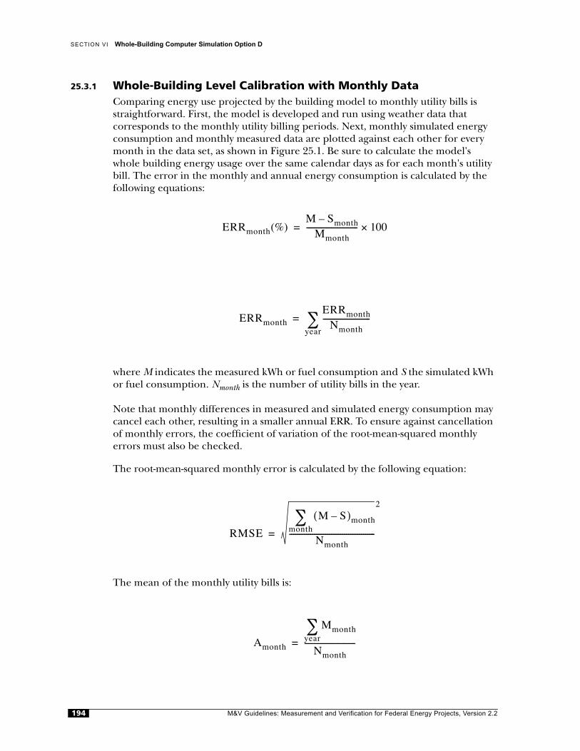
SECTION VI Whole-Building Computer Simulation Option D
25.3.1 Whole-Building Level Calibration with Monthly DataComparing energy use projected by the building model to monthly utility bills is straightforward. First, the model is developed and run using weather data thatcorresponds to the monthly utility billing periods. Next, monthly simulated energy consumption and monthly measured data are plotted against each other for every month in the data set, as shown in Figure 25.1. Be sure to calculate the model's whole building energy usage over the same calendar days as for each month's utility bill. The error in the monthly and annual energy consumption is calculated by the following equations:
where M indicates the measured kWh or fuel consumption and S the simulated kWh or fuel consumption. Nmonth is the number of utility bills in the year.
Note that monthly differences in measured and simulated energy consumption may cancel each other, resulting in a smaller annual ERR. To ensure against cancellation of monthly errors, the coefficient of variation of the root-mean-squared monthly errors must also be checked.
The root-mean-squared monthly error is calculated by the following equation:
The mean of the monthly utility bills is:
ERRmonth(%)M Smonth–
Mmonth--------------------------- 100×=
ERRmonthERRmonth
Nmonth-------------------------
year∑=
RMSE
M S–( )monthmonth∑
Nmonth---------------------------------------------
2
=
Amonth
Mmonthyear∑
Nmonth---------------------------=
M&V Guidelines: Measurement and Verification for Federal Energy Projects, Version 2.2194
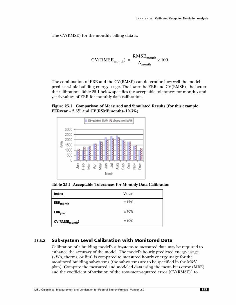
CHAPTER 25 Calibrated Computer Simulation Analysis
The CV(RMSE) for the monthly billing data is:
The combination of ERR and the CV(RMSE) can determine how well the modelpredicts whole-building energy usage. The lower the ERR and CV(RMSE), the better the calibration. Table 25.1 below specifies the acceptable tolerances for monthly and yearly values of ERR for monthly data calibration.
Figure 25.1 Comparison of Measured and Simulated Results (for this example EERyear = 2.5% and CV(RSMEmonth)=10.3%)
Table 25.1 Acceptable Tolerances for Monthly Data Calibration
25.3.2 Sub-system Level Calibration with Monitored DataCalibration of a building model's subsystems to measured data may be required to enhance the accuracy of the model. The model's hourly predicted energy usage (kWh, therms, or Btu) is compared to measured hourly energy usage for themonitored building subsystems (the subsystems are to be specified in the M&V plan). Compare the measured and modeled data using the mean bias error (MBE) and the coefficient of variation of the root-mean-squared error [CV(RMSE)] to
Index Value
ERRmonth ±15%
ERRyear ±10%
CV(RMSEmonth) ±10%
CV RMSEmonth( )RMSEmonth
Amonth------------------------------ 100×=
M&V Guidelines: Measurement and Verification for Federal Energy Projects, Version 2.2 195
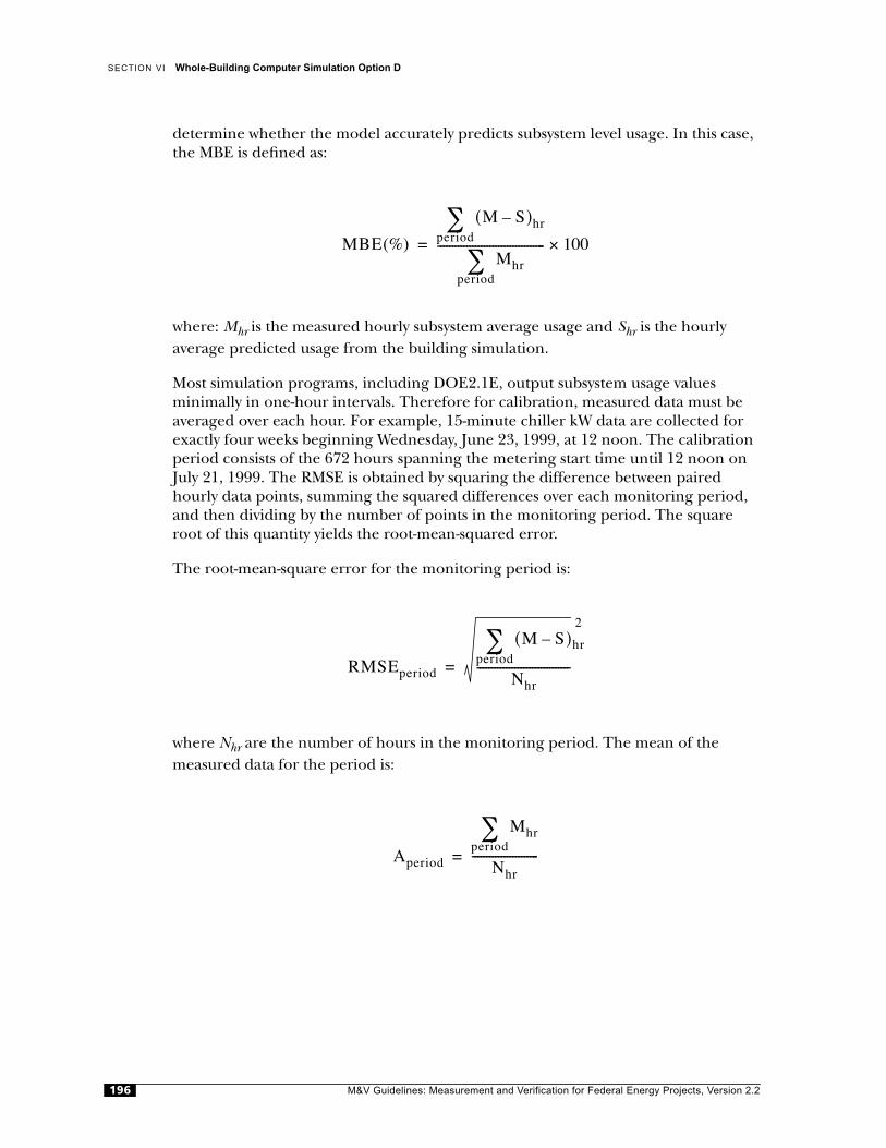
SECTION VI Whole-Building Computer Simulation Option D
determine whether the model accurately predicts subsystem level usage. In this case, the MBE is defined as:
where: Mhr is the measured hourly subsystem average usage and Shr is the hourlyaverage predicted usage from the building simulation.
Most simulation programs, including DOE2.1E, output subsystem usage valuesminimally in one-hour intervals. Therefore for calibration, measured data must be averaged over each hour. For example, 15-minute chiller kW data are collected for exactly four weeks beginning Wednesday, June 23, 1999, at 12 noon. The calibration period consists of the 672 hours spanning the metering start time until 12 noon on July 21, 1999. The RMSE is obtained by squaring the difference between paired hourly data points, summing the squared differences over each monitoring period, and then dividing by the number of points in the monitoring period. The square root of this quantity yields the root-mean-squared error.
The root-mean-square error for the monitoring period is:
where Nhr are the number of hours in the monitoring period. The mean of themeasured data for the period is:
MBE(%)
M S–( )hrperiod∑
Mhrperiod∑
------------------------------------- 100×=
RMSEperiod
M S–( )period∑
Nhr--------------------------------
2
hr
=
Aperiod
Mhrperiod∑
Nhr-----------------------=
M&V Guidelines: Measurement and Verification for Federal Energy Projects, Version 2.2196
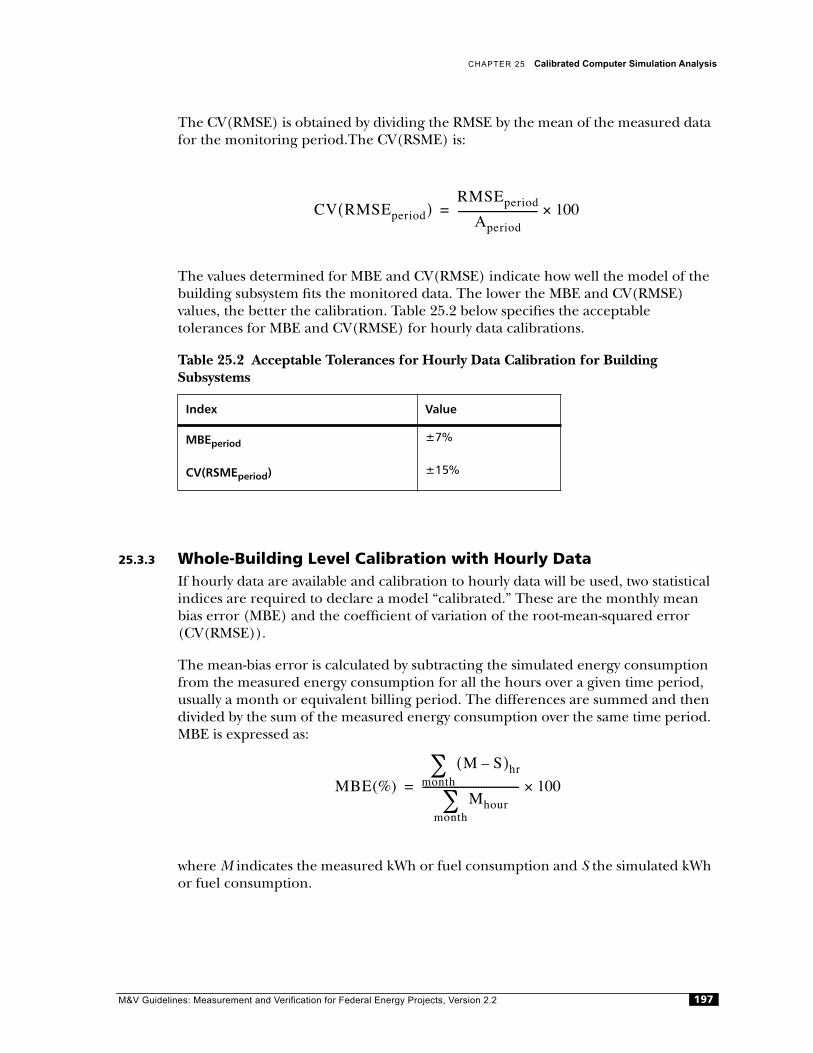
CHAPTER 25 Calibrated Computer Simulation Analysis
The CV(RMSE) is obtained by dividing the RMSE by the mean of the measured data for the monitoring period.The CV(RSME) is:
The values determined for MBE and CV(RMSE) indicate how well the model of the building subsystem fits the monitored data. The lower the MBE and CV(RMSE)values, the better the calibration. Table 25.2 below specifies the acceptabletolerances for MBE and CV(RMSE) for hourly data calibrations.
Table 25.2 Acceptable Tolerances for Hourly Data Calibration for Building Subsystems
25.3.3 Whole-Building Level Calibration with Hourly DataIf hourly data are available and calibration to hourly data will be used, two statistical indices are required to declare a model “calibrated.” These are the monthly mean bias error (MBE) and the coefficient of variation of the root-mean-squared error (CV(RMSE)).
The mean-bias error is calculated by subtracting the simulated energy consumption from the measured energy consumption for all the hours over a given time period, usually a month or equivalent billing period. The differences are summed and then divided by the sum of the measured energy consumption over the same time period. MBE is expressed as:
where M indicates the measured kWh or fuel consumption and S the simulated kWh or fuel consumption.
Index Value
MBEperiod ±7%
CV(RSMEperiod) ±15%
CV RMSEperiod( )RMSEperiod
Aperiod------------------------------ 100×=
MBE(%)
M S–( )hrmonth∑
Mhourmonth∑
------------------------------------ 100×=
M&V Guidelines: Measurement and Verification for Federal Energy Projects, Version 2.2 197

SECTION VI Whole-Building Computer Simulation Option D
The MBE indicates how well the energy consumption is predicted by the model as compared to the measured data. However, it is subject to cancellation errors, where the combination of positive and negative values for (M-S)hr serve to reduce MBE. To account for cancellation errors, the CV(RMSE) is also needed.1
The CV(RSME) is a normalized measure of variability between two sets of data. For calibrated simulation purposes, it is obtained by squaring the difference between paired hourly data points, summing the squared differences over each month orbilling period, and then dividing by the number of points, which yields the mean squared error. The square root of this quantity yields the root-mean-squared error. The CV(RMSE), is obtained by dividing the RMSE by the mean of the measured data for the month or billing period.
The root-mean-square error for the month is:
where Nhr are the number of hours in the month. The mean of the measured data for the month is:
1. Kreider, J. and J. Haberl, “Predicting Hourly Building Energy Usage: The Great Energy Predictor Shootout: Over-view and Discussion of Results,” ASHRAE Transactions Technical Paper, Vol. 100, pt. 2, June 1994.Kreider, J. and J. Haberl, “Predicting Hourly Building Energy Usage: The Results of the 1993 Great Energy Predictor Shootout to Identify the Most Accurate Method for Making Hourly Energy Use Predictions,”: ASHRAE Journal, pp. 72-81, March 1994.Haberl, J. and S. Thamilseran, “Predicting Hourly Building Energy Use: The Great Energy Predictor Shootout II, Measuring Retrofit Savings - Overview and Discussion of Results, ASHRAE Transactions, June 1996.Bou-Saada, T.E. and J.S. Haberl, “An Improved Procedure for Developing Calibrated Hourly Simulation Models,” International Building Performance Simulation Association, Report no. ESL-PA-95/08-01, 1995.
RMSEperiod
M S–( ) hr2
month∑
Nhr---------------------------------------=
Amonth
Mhrmonth∑
Nhr----------------------=
M&V Guidelines: Measurement and Verification for Federal Energy Projects, Version 2.2198

CHAPTER 25 Calibrated Computer Simulation Analysis
The CV(RSME) is:
The combination of MBE and CV(RMSE) allows one to determine how well a model fits the data: the lower the two values, the better the calibration. These indices may be calculated for the entire period, or for weekdays, weekends, and holidaysseparately (Bou-Saada and Haberl 1995). Table 25.3 below specifies the acceptable tolerances for MBE and CV(RMSE).
Table 25.3 Acceptable Tolerances for Hourly Data Calibration for Whole-Building Data
25.4 Graphical Comparison Techniques
Any or all of four graphical comparison techniques summarized in Bou-Saada and Haberl 1995 may be used to compare a simulation's output with real data. Some of these techniques require significant post-processing of data. These are:
• Hourly load profiles, which compare measured and simulated power for differ-ent day-types and seasons. These plots show where the simulation may be under- or overestimating building power.
• Binned interquartile analysis using box-whisker-mean plots, which show both measured and simulated energy use by temperature bins. Such plots allow thestatistical characterization of dense collections of points in temperature bins. These plots show how well the simulation is performing in different temperature ranges, as well as the variability in both the measured data and simulation results.
• Weather day-type 24-hour profile plots are also box-whisker-mean plots that show whole-building electricity use versus the hour-of-the-day for both measured and simulated data for different weather day-types. These plots show ambienttemperature influences and how well the simulation performs for the different weather periods chosen.
• Three-dimensional surfaces, which are plots of day, hour-of-day, and differences (positive only) between measured and simulated results (negative-onlydifferences are plotted separately). These plots show the modeler when grossdifferences occur, that may be caused by modeling errors, which can then be checked and corrected, or by building operating conditions that were not
Index Value
MBEmonth ±10%
CV(RMSEmonth) ±25%
CV RMSEmonth( )RMSEmonth
Amonth------------------------------ 100×=
M&V Guidelines: Measurement and Verification for Federal Energy Projects, Version 2.2 199
SECTION VI Whole-Building Computer Simulation Option D
accounted for in the data-collection phase of the project. Three-dimensional color plots may be used instead of surface plots. The advantage of color plots is that the plot may be easier to interpret or easier to recognize than time-of-year occurrences of peculiar data.
25.5 Calculation of Energy and Demand Savings
Whether the baseline or the post-installation building simulation is the calibrated model, total energy savings are still determined from the difference between theoutputs of the baseline and post-installation model. Savings are determined with both models using the same conditions (weather, occupancy schedules, etc.). It is very important that the baseline and post-retrofit models be consistent in terms of weather and building operation conditions (occupancy schedules, setpoints, etc.).
25.5.1 Select the Appropriate Weather Data Set and Run Both Models If savings are to be estimated for a specific year, actual weather data from that year must be used. If savings are to be estimated for a typical year, typical weather data files may be used. Both the baseline model and the post-installation model must be run with the same weather data. The weather data to be used are specified in thesite-specific M&V plan.
25.5.2 Run Models for Each ECMSo that savings are not double-counted, the ECMs should be input consecutively into the baseline model. After each is modeled, the simulation is run. The first run is the baseline model, the second run is ECM 1, the third run is ECM 1 and ECM 2, the fourth run is ECM 1, ECM 2, and ECM 3, etc. After the final ECM is input, the model should represent the post-installation condition with all ECMs installed.
25.5.3 Calculate Energy Savings. To calculate ECM energy savings, subtract energy consumption between twoconsecutive runs. To calculate total savings, subtract energy consumption projected by the post-retrofit model from energy consumption projected by the baseline model. The energy savings determined for the individual ECM should total that determined from the baseline and post-installation runs.
Savings may be quantified using the equation below. The equations are based on total energy savings determined from the difference between the baseline and post-installation runs.
Electric energy kWh savings are calculated with the equation below. Fuel savings (such as natural gas therms, oil volumes, pounds of steam,) for heating or other uses are calculated in the same manner as savings for kWh.
M&V Guidelines: Measurement and Verification for Federal Energy Projects, Version 2.2200
CHAPTER 25 Calibrated Computer Simulation Analysis
where:
kWhsaved,t = kilowatt-hour savings realized during time period t
kWhbaseline,t = kilowatt-hour consumption of the baseline building operating under the same conditions (weather, operation, and occupancy schedules, etc.) as the post-installation building, for the selected time period t
kWhpost,t = kilowatt-hour consumption of the post-installation buildingoperating under the same conditions (weather, operation and occupancy schedules, etc.) as the baseline building, for the selected time period t.
When the federal agency pays a flat fee per kWh throughout the year, t is one year and the savings calculations are straightforward. When time-of-use charges or other variable usage schedules are applied, the kWh savings must be broken down into the proper categories to determine cost savings.
25.5.4 Calculate Demand SavingsDemand savings are calculated similarly to energy savings. To calculate ECM demand savings, subtract demand between two consecutive runs. To calculate total demand, subtract demand projected by the post-retrofit model from the demand projected by the baseline model. In general, the total project demand savings is determined asfollows:
Demand savings may be based on an average demand reduction or a maximum demand reduction. Average reduction in demand is calculated as the kWh savings during the time period in question (usually the utility summer peak period) divided by the hours in the time period. Maximum reduction in demand is typically the reduction in the utility-metered maximum demand under terms and conditions specified by the servicing utility. For example, the billing peak may be based on the maximum building kW load measured in 15-minute intervals and coincident with the utility peak demand period. The maximum demand reduction is usuallycalculated to determine savings in utility peak demand charges. Thus, if utility demand savings are to be determined, each site must define (a) how the reduction will affect the utility bill and (b) how the demand reduction will be calculated for purposes of payments to the ESCOs.
kWhsaved t, kWhbaseline t, kWhpost t,–=
kWsaved kWbaseline kWpost–=
M&V Guidelines: Measurement and Verification for Federal Energy Projects, Version 2.2 201

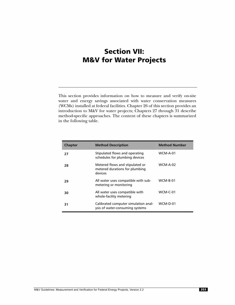
M&V Guidelines:
Section VII:M&V for Water Projects
This section provides information on how to measure and verify on-sitewater and energy savings associated with water conservation measures(WCMs) installed at federal facilities. Chapter 26 of this section provides anintroduction to M&V for water projects; Chapters 27 through 31 describemethod-specific approaches. The content of these chapters is summarizedin the following table.
Chapter Method Description Method Number
27 Stipulated flows and operating schedules for plumbing devices
WCM-A-01
28 Metered flows and stipulated or metered durations for plumbing devices
WCM-A-02
29 All water uses compatible with sub-metering or monitoring
WCM-B-01
30 All water uses compatible with whole-facility metering
WCM-C-01
31 Calibrated computer simulation anal-ysis of water-consuming systems
WCM-D-01
Measurement and Verification for Federal Energy Projects, Version 2.2 203
26Introduction to Water Conservation Measurement and Verification
26.1 Introduction
This chapter provides background information on water conservation opportunities, M&V issues relating to water conservation, and overviews of various M&V methods that follow the framework of Options A, B, C, and D. Some of the information and text in this section comes directly from the 1997 version of the InternationalPerformance Measurement and Verification Protocol (IPMVP). The IPMVP (see www.ipmvp.org) contains additional information and references that may be useful in developing water conservation projects and plans for measuring and verifyingsavings.
26.2 Water Conservation Measures
Water resource efficiency has become one of the most successful tools that water and sewer providers can use to limit and manage the increasing costs of providing water and treating wastewater. A partial list of water conservation measures that Federal agencies can consider includes the following:
• Replacing components of older plumbing systems with water-saving equipment such as ultra-low-flow toilets (ULFTs), high-efficiency shower heads, aerators, and self-closing valves.
• Eliminating continuously flowing urinals, lab drains, drinking fountains, and other similar devices.
• Replacing once-through cooling devices for space-cooling, icemaking, and other purposes with closed-loop or air-cooled systems.
• Improving technologies and management techniques for boilers, dishwashing, laundry, and other special purposes.
• Identifying and repairing all leaks promptly (an operations and maintenance measure.
• Maintaining proper pressure through the use of pressure regulating valves (PRVs).
• Decreasing the use of water for landscaping by implementing xeriscaping and more efficient irrigation systems and practices.
M&V Guidelines: Measurement and Verification for Federal Energy Projects, Version 2.2204

CHAPTER 26 Introduction to Water Conservation Measurement and Verification
• Installing graywater, rainwater, and reclaimed water-recycling technology for flushing and/or irrigation
• Installing monitoring equipment and sub-meters as needed so that increases in consumption over time can be quickly rectified
On-site savings, or savings that accrue directly to the facility, can result from reduced water supply charges, sewer charges, and/or energy costs.The greatest savings are often the result of lowered energy costs, for example, reduced water heating,pumping, and treatment needs. Energy savings often occur at facilities that use pumps to boost water pressure or to irrigate with groundwater, or at facilities with their own water-treatment systems.
In some warm, humid climates, hot water is also used to temper cold water in toilet and urinal cisterns in order to prevent condensation problems. In some very coldclimates, hot water is bled into cisterns and cold water pipes to prevent freezing problems. Although fixture retrofits may greatly reduce hot water needs for these purposes, it is generally preferable not only to retrofit the fixtures, but also to reduce or eliminate the need for hot water by using strategies such as insulating cisterns and pipes, using passive solar techniques to heat cold water pipes (which can also reduce cooling loads), and other techniques.
Unfortunately, certain water measures may actually increase on-site energy use. For example, switching from a once-through cooling system to a closed-loop or air-cooled system can greatly reduce water usage, but it requires fans or pumps andcan lower cooling efficiency, depending on the temperature of the incoming water. Agencies should take such increases in energy demand into account whendetermining overall savings accruing to a specific site.
On-site water conservation can also result in off-site energy savings. Though federal performance contracts will not include payments for these savings, there may be value in considering them for utility incentive programs.
26.3 Information on Federal Water Conservation Programs
The Energy Policy Act of 1992 (EPAct) and Executive Order 13123 call for theimplementation of water conservation projects and provide the authority to useperformance contracting to finance these projects. Subtitle F, Section 152, of EPAct amends Section #541 of the National Energy Conservation Policy Act (42 USC 8252) to explicitly include water with the requirement related to energy use. The samesection also directs federal agencies to install in the facilities they own, to themaximum extent practicable, all energy and water conservation measures with apayback period of 10 years or less. Subtitle F, Section 152, of EPAct amends 42 USC 8287 to authorize the use of energy-saving performance contracting, and Section 152 authorizes and encourages agencies to participate in incentive programs offered by gas, water, or electric utilities to finance the installation of energy and waterefficiency measures required by EPAct.
M&V Guidelines: Measurement and Verification for Federal Energy Projects, Version 2.2 205

SECTION VII M&V for Water Projects
Executive Order 13123, “Energy and Water Efficiency in Federal Facilities,” Section 303, further directs agencies to identify conservation opportunities and installcost-effective conservation measures. Finally, Section 401 directs agencies to useinnovative financing and contractual mechanisms including, but not limited to,utility demand-side management programs and energy-savings performancecontracts to meet the water and energy goals and requirements.
DOE's Federal Energy Management Program (FEMP) is working with federalagencies to help achieve these goals. FEMP provides technical support to federal facility managers to help identify opportunities for successful water conservation projects. FEMP's technical assistance program offers a range of services, including project and financing assistance, software tools, and training.
Federal Water Working GroupsThe Federal Water Working Group, established by the Interagency EnergyManagement Task Force and facilitated by the FEMP Water Conservation Program, focuses on water management awareness, technical assistance, training, waterconservation plan development, and partnerships with industry and professional associations. The Federal Utility Partnership Working Group consists ofrepresentatives from water, wastewater, electric and gas utilities, and federalagencies. The group explores ways that federal agencies and utilities can work together to create efficiency projects and programs that benefit all parties.
Project AssistanceFor site-specific projects, FEMP can help plan and develop projects, leverage resources, and provide information on water-efficiency technologies. As part of the project-screening process, FEMP has developed WATERGY, a spreadsheet modelthat uses water/energy relationship assumptions to estimate potential water and associated energy savings at a facility or building.
Project Financing AssistanceThe FEMP Water Conservation Program also supports federal agency use ofalternative financing mechanisms. These include ESPC and utility contracts for water conservation projects.
Training and WorkshopsFEMP offers a Water Resource Management training course and, for a fee, can design and implement agency-specific water conservation workshops. Traininginformation and WATERGY software, copies of water conservation case studies, and other information resources can be obtained from the FEMP Help Desk.
26.4 M&V Options for Water Conservation Measures
This part provides a brief overview of methods for determining water savings. The methods follow the framework of the IPMVP's Options A, B, C, and D. An overview of the M&V options is presented in Chapter 2.
M&V Guidelines: Measurement and Verification for Federal Energy Projects, Version 2.2206
CHAPTER 26 Introduction to Water Conservation Measurement and Verification
The four M&V options for WCMs are as follows:
• Option A: Focuses on physical assessment of equipment and system changes to ensure that installation is to specification. Key performance factors (e.g., gallons per flush) are determined with spot measurements or manufacturer's data, and operational factors (flushes per hour) are stipulated based on an analysis ofhistorical data and/or one-time, spot, or short-term measurements.
• Option B: Savings are determined after project completion by using short-term or continuous measurements taken throughout the term of the contract at the device or system level. Both performance and operational factors are monitored.
• Option C: Savings are determined after project completion at the whole-building or facility level using current-year and historical utility meter or sub-meter data.
• Option D: Savings are determined through simulation of facility components and/or the whole facility. The simulation is calibrated with end-use or whole-facility metering data. Simulations can include anything from spreadsheets using fixture unit data to sophisticated programs using psychometric calculations.
M&V methods defined for these options are summarized in part 26.7.
26.5 Water Conservation M&V Issues
26.5.1 M&V Cost ConsiderationThe value of a WCM should be considered when deciding how much effort to put into M&V activities. The value of the M&V information should not exceed the cost of obtaining the information. Thus, when examining water efficiency opportunities with small amounts of water savings, ESCOs and federal agencies may need to apply simplified versions of the M&V techniques used for energy efficiency. Exceptions to this approach exist when the water-efficiency projects lead to significant direct or indirect energy savings.
26.5.2 Water RatesWater and sewer rates vary tremendously throughout the country. Many locations do not charge on the basis of consumption and/or do not meter the service. Otherjurisdictions charge only for water consumption and issue a flat bill for sewerservices. Most areas, however, bill for water and sewer service from meter readings, and a large percentage of charges are consumption based. These are areas where performance contracting can be most successful for all parties involved.
As with energy-efficiency projects, the goal of a performance contract is to reduce facility operating costs. The M&V approach selected should be designed to provide water and energy savings information in such a way that cost savings can beestimated. Therefore, the M&V plan should ensure that:
M&V Guidelines: Measurement and Verification for Federal Energy Projects, Version 2.2 207
SECTION VII M&V for Water Projects
20
• Appropriate energy, water, and sewer rate schedules are used to calculate costsavings.
• Agreements are made between the federal agency and the ESCO on how changes in rates (e.g., $/1000 cubic feet) and changes in how the charges are calculated (flat rate changed to volumetric rate) will affect any savings guarantees or shared savings arrangements.
• The water (and energy) savings data and calculations can be used to determine cost savings—i.e., all the data used to calculate a water, sewer, and energy bill are available and documented.
26.5.3 Meter Accuracy and Metering The quality and accuracy of water meters varies significantly according to the type, initial quality, age, calibration efforts, and maintenance of individual meters. Ahistorical consumption level could be substantially lower than actual flow. The encoded register meters used by most water utilities tend to register anywhere from zero to 25% low (IPMVP, Section 4.5.1) and thus may not precisely representconsumption after long periods of service. Therefore, using historical water meter data may not provide an accurate baseline for purposes of a performance contract and can adversely affect savings projections.
Recommendations for metering include the following:
• All meters installed to verify savings should comply with appropriate American Water Works Association (AWWA) accuracy standards. Regular calibration should be part of any M&V plan that relies on the use of either whole-facility or sub-meters for the calculation of savings.
• Sub-meter quality must be addressed if these meters are used to measurequantities involved in determining savings. Degradation of low-quality meterscan result in artificially low flow readings.
• If existing water meters are used in the M&V effort, project partners shouldconsider either testing the accuracy of the meters or installing metersindependent of the utility meters. For example, adjusting three years of istorical water-use data, based only on recent calibration may not accountproperly for meter inaccuracies that varied throughout the last three years.
Flow measurements can be made either with flow meters or by volumetric means. Suitable flow meters are selected for appropriate accuracy and have flow ratings that conform to field conditions. Flow rates can also be determined by measuring how much water (i.e., its volume) is used or discharged during a measured time interval. For example, water discharged from a faucet is collected for a timed period of2 minutes, and is found to be exactly 5 gallons when measured; the flow rate is5 gallons divided by 2 minutes, or 2.5 gpm (gallons per minute). Volumetricmeasurements are usually used to determine how much water is discharged during a set cycle, such as one flush of a water closet. Dishwashers and clothes washers also have set cycles, although care must be taken to recognize possible variations such as water-saver cycles or extra rinse cycles.
M&V Guidelines: Measurement and Verification for Federal Energy Projects, Version 2.28
CHAPTER 26 Introduction to Water Conservation Measurement and Verification
Spot measurements are useful not only to quantify water consumption but also to make sure specific devices are assigned to appropriate groups (when sampling is used to characterize the entire population of devices) and to verify that all devices assigned to the sampling group have similar performance characteristics.
Flow measurements should be made with integrating flow meters, either by direct reading or perhaps through an energy management system (EMS), and with orwithout automatic recording. Suitable flow meters will be selected for appropriate accuracy and have flow ratings that conform to field conditions. The readout from integrating flow meters will be in volumetric units, typically gallons or cubic feet, often with a multiplier. Knowledge of the correct multiplier is critical. Readings must be taken and recorded regularly, either monthly or at a more frequent interval.
Fixtures of a similar type that have the same flow characteristics can be grouped together. Units of measure should be consistent with the fixture type, but all should be expressed with a common volumetric measure (usually gallons) so those totals can be aggregated easily. For example, water consumption for water closets might be expressed in gallons per flush, while shower consumption is expressed in gallons per minute. Water consumption per unit of measure must then be quantified in the same units, and periods of service must be expressed in consistent terms (such as flushes per day, or minutes per shower and showers per day). In some facilities the utilization factor may change seasonally (e.g., a school summer vacation period);separate data will be needed for each season.
26.5.4 Nameplate DataESCOs and agencies should use great caution if they rely on nameplate data for M&V calculations of baseline water-use or savings. The water consumed by most water fixtures can be easily adjusted to go well above or below nameplatespecification. Actual use for existing fixtures can be determined by short-termmetering or other techniques. All newly installed equipment should be tested and adjusted as needed.
The following are two examples (excerpted from the 1997 IPMVP, Section 4.5.1):
ToiletsExisting toilets that are nominal five-gallon-per-flush (GPF) models (pre-1980) are often assumed to consume 4.5–5.0 GPF. “Low-flush” toilets from the 1980s aregenerally said to have a nominal flush volume of 3.5 gallons. These assumptions are not always valid, because significant variations are possible due to internal refillsettings and different flush mechanisms. The flush volume of “flushometer” valve toilets may vary by as much as several gallons depending on water pressure, valve condition, and, in the case of piston-type flush valves, the position of the adjustment screw. Even gravity tank toilet flush volumes may vary somewhat with watertemperature and pressure, although these variations may be relatively minor.
M&V Guidelines: Measurement and Verification for Federal Energy Projects, Version 2.2 209
SECTION VII M&V for Water Projects
21
M&V Guidelines: Measurement and Verification for Federal Energy Projects, Version 2.20An assumption must also be made for the number of flushes per day. This isparticularly difficult since it requires an understanding of how building occupants live and work and how often they “double-flush” the toilet. Although there has been much discussion of the need to double-flush low-consumption toilets, some informa-tion indicates that higher-consumption toilets are being double-flushed as well.
The actual measured consumption of “water-wasting” toilets varies from 3.5–7 GPF. A stipulation of unit flush volumes for existing toilets ignores the fact that a part of the baseline consumption and later water savings resulting from toilet replacement(or repair/retrofit of existing toilets) comes from ending internal leaks in the oldtoilets. These leaks can originate with seeping/leaking flappers, ball cocks out ofadjustment, leaking supply lines, etc. Leaks can be identified by using techniques such as dye tablets in toilets or looking for variances from normal consumption rates. Quantifying baseline losses due to leaks is difficult, however, and simple stipulations should be used with caution.
Shower HeadsExisting pre-1990 shower heads are often assumed to flow at 5 gallons per minute (GPM). However, field studies suggest that actual flow rates are closer to 4 GPM, and sometimes even lower. Flow rates may vary, depending on the specific shower head model, water pressure, and condition of the fitting, from well over 5 GPM to less than 1 GPM. The flow rates of most older shower heads vary significantly with water pressure and long-term deposition. Of course, an assumption must be made about the number and duration of showers per day.
Taking Spot Flow Measurements of Shower Heads and ToiletsTaking spot flow measurements of shower heads and toilets can be done by using small flow meters or by timing the filling of a container of known volume. Unliketoilets, for which measuring unit flush volumes involves the often difficultinstallation of inline flow meters on water lines, approximating showered flowrates can be accomplished by using a graduated container or calibrated measuring device (e.g., the Water Weir), which does not require a timer. After determining flow rates and flush volumes, an assumption must still be formulated concerning usage rates (number of flushes per day, number and duration of showers per day).
26.5.5 Baseline AdjustmentsBaseline adjustments, which may be required during the service phase of an ESPC, are a common area of contention in performance contracts. In general, one might expect baseline adjustment changes to fall into one or more of the following three categories:
1. Clearly expected and predictable annual variations. For example, changes in rainfall that affect irrigation requirements or changes in a building's occupancy that affects water closet use. These are usually dealt with through defined proce-dures for each identified factor in the savings formulas. Such procedures might include the use of regression analyses to calculate savings using current-year weather or occupancy data (Options B and C), stipulating the use of typical weather or occupancy data (all options), or agreements to modify baseline calcu-lations by using current-year weather or occupancy data (Options A and D).

CHAPTER 26 Introduction to Water Conservation Measurement and Verification
2. Potential changes that are predictable, although describing a detailed calculation method for them is not reasonable given the unknowns about each situation or the cost of developing numerous “what-if” scenarios. For example, adding more occupancy hours to a library, closure of a facility, adding new wings on a hospital, or acquiring more landscape irrigation acreage. These changes require aconceptual approach defined in the agreement between the ESCO and the agency, rather than a method to cover each eventuality. Examples of suchconceptual approaches are (a) defining which party is responsible for decreases in energy-savings associated with different categories of changes, (b) defining whether an ESCO is able to claim credit for additional savings associated withdifferent categories of changes, (c) defining the categories of changes eligiblefor baseline adjustments, (d) defining which party can request a baselineadjustment, and (e) when this can be done, what time period of the servicephase the adjustment will cover, and what approval process is required.
3. Potential changes that are not obviously predictable. For example, changing the use of a facility from warehouse to office space. These potential changes require either (a) agreement clauses that allow for adjustments for unexpected changes and/or (b) the use of a “re-open” clause that allows either party to renegotiate the baseline “model.” These clauses would be part of or consistent withtermination, default, and arbitration clauses contained in the agreement between the agency and the ESCO. Determining which of the these threecategories each potential change fits into can be done by preparing a list of potential changes associated with each water conservation measure or bydefining which baseline factors are constant or are assumed to be constant,and which can vary.
The following are some notes on baseline adjustments:
• Even if utility meter analysis is used to determine savings, a complete and detailed audit (e.g., investment-grade audit) is required. If the baseline conditions are not well documented, it becomes difficult, if not impossible, to properly adjust them when they change and adjustments to payment calculations are required. For example, if a toilet valve retrofit takes place in a building with 100 toilets, and later (during the service phase) the number of toilets is increased to 125, post-installation water-use may be more and calculated savings may be less. If there were no records of how many toilets were originally in place, however, thebaseline could not be adjusted to properly reflect the amount of “true” savings and how much the ESCO should be paid.
• With Option A, baseline adjustments are less likely to be required because many of the factors are stipulated, such as occupancy. This is one reason why Option A can be less accurate but easier and less expensive to implement.
• Option B involves metering techniques. Baseline capacity values are assumed to be constant (e.g., baseline sprinkler head flow rates or water closet gallons per flush), but baseline “operating values” can be changed by using post-installation monitoring data (e.g., hours per year of irrigation and flushes per day).
M&V Guidelines: Measurement and Verification for Federal Energy Projects, Version 2.2 211
SECTION VII M&V for Water Projects
• For Option C, billing analysis, either typical values or post-installation values are defined for baseline and post-installation independent variables that influence water-use (e.g., weather and occupancy). It is important to agree in advance on the variables that will be used.
• For Option D, calibrated simulation, it is important to agree in advance on the model to be calibrated and what changes will require a new simulation run. For most retrofit and new construction projects, baseline and post-installation models are calibrated and then run with typical input data (e.g., weather data). Thereafter, they are typically not modified unless major changes occur at thesite. Annual verifications are expected, but normally the models do not need to be run again unless changes occur to the installed WCMs.
26.5.6 Notes on Outdoor Water Use
Establishing Baseline Water ConsumptionUnless there is a separate meter of outdoor water use, the usual first step is toevaluate the entire facility's water consumption by using several years of data tocompare seasonal irrigation use with non-seasonal irrigation use. The difference can be used for a baseline but should be adjusted for changes in temperature, rainfall, evapotranspiration, and/or other relevant factors, if possible. If the water utilityseparately meters outdoor water use, then establishing baseline use is relativelysimple, except for concerns regarding the accuracy of older utility meters. Thedifficulty with monitoring whole-building consumption is that outdoor water use can be so variable that desegregating that end-use from a facility's water load, which is itself variable in use, can be problematic.
If outdoor end uses are not separately metered by the water utility, strongconsideration should be given to installing new meters to track outdoor end uses.
An alternative to establishing baseline outdoor use, without new or existingmetering, depends on the system having a relatively constant flow rate and being operated on a relatively regular schedule. For example, the consumption of asprinkler system that flows constantly at “X” cubic feet per minute (CFM) for “Y” hours per day can be reasonably estimated. It is common, however, for operators to vary the operation of outdoor systems, depending on perceptions of need. Detailed information about how the system is operated is necessary to place a high degree of confidence in calculated estimates of use, unless the investment in the project is small enough to tolerate a relatively low degree of confidence in the estimate ofbaseline use.
Methods of Monitoring SavingsIn comparison to metered observations, estimating savings from outdoor water-use projects by stipulating or assuming changes in the system's operation is particularly difficult. Efficiency improvements to outdoor water end-uses generally are focused on either modifying the schedule of irrigation or improving the efficiency of water delivery to the lawn or crops.
M&V Guidelines: Measurement and Verification for Federal Energy Projects, Version 2.2212
CHAPTER 26 Introduction to Water Conservation Measurement and Verification
Modifying the schedule of irrigation is based on varying irrigation times with weather and the evapotranspiration rate. These savings may be specific to the plant species involved and certainly vary according to the region and even the microclimate. Increasing the delivery efficiency of water involves the use of irrigation technologies (e.g., “drip irrigation” or more efficient sprinkler technologies) or other changes that result in lower evaporative losses. These savings also depend on local climate and evapotranspiration rate as well as plant species. Even metered baseline and post-retrofit data may need to be “normalized” with changing weather.
26.5.7 Notes on Graywater Use
Establishing Baseline ConsumptionEstablishing baseline consumption depends on which end use(s) the graywater isdisplacing. The two most common end uses are irrigation and toilet/urinalflushing. In each case, the whole-facility meter, end-use metering, or stipulation approaches for assessing baseline consumption can apply.
Methods of Monitoring SavingsIf graywater is completely displacing potable water for a specific end use, and the graywater consumption level can be shown to represent a one-to-one correlation to that of the displaced potable water, then the complications of determining a baseline are not an issue. For post-installation graywater measurements, it may be easier to meter the flow of graywater into a system. If the graywater originates from multiple sources, then it would be easier to monitor the use of graywater at the end use.
26.5.8 Demand SavingsSome water utilities have demand charges that are linked to water meter size. Water conservation projects therefore may not realize any demand savings unless the water meter is replaced with a smaller one, or if it can be shown that a larger meter would have been required in the absence of the WCMs. In these situations, any demandsavings will depend on the change in meter size and the serving utility's schedule of charges.
Changes in water supply demand may also affect sewer charges. Sewer charges are sometimes based on how much water is delivered to the utility's supply meter during a specified period, such as one winter month. Demand savings from reduced sewer charges resulting from water conservation measures can be calculated from the sewer charge before and after the improvements are made.
26.5.9 Sanitary ConsiderationsMost domestic water use is for cleaning and transporting waste. These are sanitary functions that use equipment and systems designed to comply with carefully crafted sanitary codes and standards. Saving water by using methods that compromise system performance is unacceptable. For example, when graywater systems are installed, special attention should be taken to prevent cross connections and prolongedretention periods.
M&V Guidelines: Measurement and Verification for Federal Energy Projects, Version 2.2 213
SECTION VII M&V for Water Projects
26.6 General Considerations for Selecting an Appropriate M&V Option and Method
26.6.1 Whole-Building Analysis—Option CThe most common approach to M&V for water is the “whole-building” or main-meter approach, in which all aspects of water usage are combined into a single M&V analysis strategy.
To establish a baseline figure on which all savings calculations are based, a typical method is to average the previous 2 to 3 years of consumption data (e.g., directly from past water/sewer bills) and convert this number into daily usage. Thiscalculation will typically be in gallons, but it can also be in cubic feet or cubicmeters. The baseline figure will be in units of water/sewer use (e.g., average daily consumption), which is not a monetary amount. During the term of theperformance contract, this baseline figure can be converted into a monetaryamount using the current water/sewer rate in that community.
Understanding and tracking key parameters at the facility (e.g., population changes) are important in accurately defining a baseline and estimating building-wide water savings estimates. These parameters are used in adjusting the baseline as theparameters change over time.
As an added benefit, detailed and frequent (even continuous) building-wide water consumption metering data may also provide important information for assessing equipment performance.
26.6.2 Sub-meters and Data Loggers—Option BWater sub-metering should be considered for the following:
• Facilities with significant single process use or outdoor water use.
• Large facilities with distinct water-use areas that can be accurately metered and monitored; examples include individual buildings on military bases, coolingtowers, laundry facilities, or graywater systems.
• Facilities for which the agency wants to achieve or verify savings for a discreteportion.
One benefit of sub-metering is that it provides ongoing information on theperformance of individual systems. This can provide the federal agency and ESCO with early warnings of system problems, and it may prove helpful if troubleshooting is required. For example, a leak that could easily nullify all water savings resulting from a water measure can be more easily identified and repaired by regular reading of submeters.
M&V Guidelines: Measurement and Verification for Federal Energy Projects, Version 2.2214
CHAPTER 26 Introduction to Water Conservation Measurement and Verification
Water sub-metering should be considered in order to make the user (e.g., individual departments) accountable for his or her water use. For example, reductions in water consumption are being experienced in multifamily properties that use sub-metering as a conservation strategy. Thus, water sub-metering can both promote savings and act as a means of detailed verification.
Sophisticated water meter data loggers have been developed that can greatly assist in the M&V of water measures. The use of data loggers can often help identify actual savings when a facility faces considerable and/or uncontrollable changes in factors that affect water use (e.g., occupancy, weather). Changing factors can often be too expensive and nearly impossible to measure. With data loggers, water savings perfixture use can be measured rather than relying on the measurement of overall reductions in water use.
26.6.3 Use of Stipulations—Option AAs discussed in part 26.5.4 using nameplate data for water-consuming devices can introduce significant uncertainty into savings calculations. Thus, this approach should be used with caution and only for projects in which the economic value is low, where there is little risk of not obtaining the project, and/or for which assumptions can be tested or confirmed with current or historical data.
While a stipulation may be the least expensive method of determining post-installation unit consumption rates, water savings calculations still have a significant variable—the number of uses (e.g., flushes, showers, irrigation schedule, and their duration).
26.6.4 Use of Simulation Tools—Option DThis M&V approach can be considered a combination of Options A and B or A and C, in which meter data are combined with calculations using analysis tools such as spreadsheets, vendor computer programs, or sophisticated simulation programs that estimate water use in evaporative cooling systems, for example. Caution should be used when working with any simulation tool to ensure that the results are reasonable and documented. See Chapter 24 for general information on calibrated simulation for energy efficiency projects.
26.6.5 Using Multiple M&V Options at a Single FacilityWhen a variety of measures are installed at a single facility, it is not recommended that different M&V options be used to calculate savings. For example, Option B should not be used to calculate savings from an irrigation retrofit when Option C is then used to calculate the remaining savings at a facility, through a billing meter analysis and the subtraction of the irrigation system savings. This can lead toinaccuracies in savings estimates.
M&V Guidelines: Measurement and Verification for Federal Energy Projects, Version 2.2 215
SECTION VII M&V for Water Projects
26.7 Summary of M&V for Water Conservation Measures
The following paragraphs and tables summarize the five M&V methods described in this document as they apply to WCMs. Each method is appropriate for differentmeasure types and risk profiles. The descriptions in this document assist federalprocurement and project managers as well as ESCOs in the selection of the most appropriate method. See part 26.6 for a discussion on selecting appropriate M&V methods.
26.7.1 Method WCM-A-01—Stipulation of Key Variables, No MeteringThis method assumes that the federal agency and the ESCO are confident that unit water consumption can be defined and stipulated for each fixture type and that device usage schedules (flushes per month, hours of use, water schedule, or another parameter) can be quantified and stipulated based on the manufacturer's data and other available data. This M&V method is appropriate for projects in which water is conserved in either or both of these ways:
• Replacing existing plumbing fixtures (the baseline) with new fixtures designed to deliver water at low flow rates
• Delivering water during fewer and/or shorter intervals.
Example WCMs include new toilets, urinals, shower heads, and/or irrigation head retrofits; defined-cycle laundry and dishwashing retrofits; and irrigation and once-through pumping control conversions.
In this approach, as with all M&V methods, surveys are required to documentexisting (baseline) and new (post-installation) devices and their characteristics.
All values, however determined, are stipulated for the term of the agreement, subject to changes in the facility or its operation. The source(s) of stipulations may vary and can include manufacturers' ratings, published values for a range of flows typically associated with a given generic type of plumbing fixtures, and results from prior projects.
Water consumption savings are based on the following:
• Stipulated baseline consumption for each type of device
• Stipulated post-installation consumption for each type of device
• Number of devices, both baseline and post-installation, of each type
• Stipulated cycles or hours per year for each operating scenario, both baseline and post-installation.
M&V Guidelines: Measurement and Verification for Federal Energy Projects, Version 2.2216
CHAPTER 26 Introduction to Water Conservation Measurement and Verification
26.7.2 Method WCM-A-02—Stipulation of Key Variables Using Spot or Short-Term MeteringThis method is the same as method WCM-A-01 except that one-time, spot, or short-term metering is used to quantify key parameters. This method is used if the federal agency and ESCO want to verify savings with the simplicity associated with Option A, but also want to base stipulations on metering data. Thus, either or both of these can be done:
• Values for baseline and post-installation flow rate are determined one time with either spot measurements (e.g., averaging four measurements of representative toilets' water flow per flush) or short-term measurements (e.g., the average of two weeks of values to determine average daily flow rate for a sprinkler system).
• Operating hours or cycles per time period are determined with short-termmetering.
Water consumption savings are based on the following:
• Baseline consumption for each type of device, based on metering data or other sources
• Post-installation consumption for each type of device, based on metering data or other sources
• Number of devices, both baseline and post-installation, of each type
• Stipulated cycles or hours per year for each operating scenario, both baseline-based and post-installation-based, using short-term metering or historical data.
26.7.3 Method WCM-B-01—Determining Savings from Plumbing Fixture and Other Water-Consuming-System Retrofits with the Use of Sub-MeteringThis method is applicable to retrofits in which all or a sample of affected devices' (or systems') water consumption can be sub-metered and/or monitored. Because of the costs of this method, it is recommended for retrofits associated with the following: (a) water closets, urinals, irrigation, etc., with electronic controls that can be used to record operating patterns, or (b) systems that are already, or can easily be, sub-metered.
Examples of these measures are irrigation system retrofits and large-scale shower head retrofits in a locker room setting.
In this approach, as with all M&V methods, surveys are required to documentexisting (baseline) and new (post-installation) devices and their characteristics.
M&V Guidelines: Measurement and Verification for Federal Energy Projects, Version 2.2 217
SECTION VII M&V for Water Projects
Water consumption savings are based on the following:
• Number of devices, both baseline and post-installation, of each type
• Measured baseline consumption, extrapolated to annual values, for each device or device category
• Measured (either continuously or during representative time periods and then extrapolated to annual values) consumption for each device or device category
• Baseline device counts, cycles, or hours of use are updated, as needed, using regressions/correlations with independent variables (e.g., occupancy and weather).
26.7.4 Method WCM-C-01—Determining Savings from Plumbing Fixture and Other Water-Consuming-System Retrofits with the Use of Whole-Facility MeteringThis method is applicable to all water system retrofits when project consumption and/or water savings are large in comparison to the total consumption recorded on whole-facility meter(s). Because of this limitation, this method is recommended for water system retrofits that are large and comprehensive.
Examples of measures are graywater applications and large-scale plumbing fixture retrofits.
In this approach, as with all M&V methods, surveys are required to documentexisting (baseline) and new (post-installation) devices and their characteristics.
Water consumption savings are based on the following:
• Historical whole-facility water meter and independent variable (e.g., weather or occupancy) data
• Recorded whole-facility, post-installation consumption, and independent variable data
• Regression analysis to isolate the effects of the WCM from the other variables.
26.7.5 Method WCM-D-01—Determining Savings From Plumbing Fixture and Other Water-Consuming-System Retrofits with the Use of Cal-ibrated Simulation AnalysisThis method is applicable to retrofits in which baseline and post-installation water-use can be simulated and the simulation can be calibrated using whole-facility and/or end-use metering data. Because of the possible complexity and costs associated with this method, it is recommended for comprehensive retrofits for which Options B or C cannot be applied because of complex interactions and/or the effects ofindependent variables.
M&V Guidelines: Measurement and Verification for Federal Energy Projects, Version 2.2218
CHAPTER 26 Introduction to Water Conservation Measurement and Verification
Examples of these measures are cooling tower retrofits and other HVAC types of projects.
In this approach, as with all M&V methods, surveys are required to documentexisting (baseline) and new (post-installation) devices and their characteristics.
There are several approaches for determining savings using simulation models. One approach involves the following:
• Simulation of the baseline system and then calibration of this simulation with end-use or whole-facility meter data
• Simulation of the post-installation system and then calibration of this simulation with end-use or whole-facility meter data
• Comparison of the baseline and post-installation models using actual or typical independent variables (e.g., occupancy and weather).
26.8 Pre- and Post-Installation Submittals
For each site, the ESCO submits a project pre-installation report that includes the following:
• A project description and schedule
• A pre-installation equipment survey
• Estimates of water savings
• Documentation of historical water utility billing data
• Site-specific M&V plan
• Schedule of project and M&V activities.
If the federal agency defines the baseline condition, the ESCO must verify anagreed-to pre-installation equipment survey.
The ESCO submits a project post-installation report following project completion and in that document defines projected savings for the first year. In addition, the report includes many of the components as in the project pre-installation report, adding information on actual rather than expected WCM installations.
The site-specific M&V approach may be prespecified in the ESPC between thefederal agency and the ESCO and/or agreed to after the award of the project. In either case, before the federal agency approves the project construction, the ESCO must submit a final M&V plan that addresses the following:
• Overview of approach
• Specification of savings calculations, including units of measure
M&V Guidelines: Measurement and Verification for Federal Energy Projects, Version 2.2 219

SECTION VII M&V for Water Projects
• Specification of data collection methods, schedules, equipment, and reporting format
• Identification and resolution of any other M&V issues.
26.9 Site-Specific M&V Plan
Every project or, as appropriate, group of similar projects must have an approved site-specific M&V plan before the installation of any WCMs. The minimumrequirements for preparing a site-specific M&V plan, using a method described in these Guidelines, are as follows:
1. State which M&V method (chapter) of the M&V Guidelines will be used.
2. Describe the facility and the project and include information on how the project saves water (and energy) and what key variables affect the realization of savings.
3. Indicate who will conduct the M&V activities and prepare the M&V analyses and documentation.
4. Define the details of how calculations will be made. For instance, “List analysis tools and/or show the equations to be used.”
5. Specify what metering equipment will be used, who will provide the equipment, its accuracy and calibration procedures, and how data from the metering will be validated and reported, including formats; electronic format data directly from a meter or data logger is required for any short- or long-term metering.
6. Define what key assumptions will be made about significant variables or unknowns. For instance, “actual weather data will be used, rather thantypical-year data,” or “water consumption will be metered for one full year for two of the six restrooms.” Describe any stipulations that will be made and the source of data for the stipulations.
7. Describe any sampling that will be used, why it is required, sample sizes,documentation on how sample sizes were selected, and information on howrandom sample points will be selected.
8. Define the level of accuracy which should be achieved if not for the entireanalysis, at least for key components. For instance, “Irrigation water flows will be measured at a sample of locations sufficient to provide a 90% confidence level and 10% precision.”
9. Indicate how quality assurance will be maintained and repeatability confirmed. For instance, “The data being collected will be checked every month,” or “To ensure accuracy, results will be subjected to third-party review by the XYZCompany.”
10. Indicate which reports will be prepared, what they will contain, and when they will be provided.
M&V Guidelines: Measurement and Verification for Federal Energy Projects, Version 2.2220

CHAPTER 26 Introduction to Water Conservation Measurement and Verification
If the site-specific M&V plan is to be developed independent of a method described in the M&V Guidelines, then the following information is required in place of item 1 above:
• Explain why none of the M&V methods in the Guidelines is applicable.
• Provide an overview of the method.
• Describe how baseline and post-installation inventories and equipment/system descriptions will be documented.
• Describe any spot, short-term, or long-term metering that will be conducted.
• Specify the analysis method for calculating savings.
M&V Guidelines: Measurement and Verification for Federal Energy Projects, Version 2.2 221
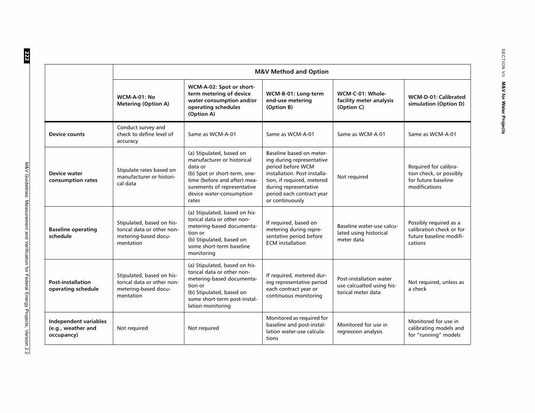
SE
CT
ION
VII
M&
V fo
r Water P
rojects
M&
V G
uidelines: Measurem
ent and Verification for F
ederal Energy P
rojects, Version 2.2
22
2
M&V Method and Option
WCM-A-01: No Metering (Option A)
WCM-A-02: Spot or short-term metering of device water consumption and/or operating schedules (Option A)
WCM-B-01: Long-term end-use metering (Option B)
WCM-C-01: Whole-facility meter analysis (Option C)
WCM-D-01: Calibrated simulation (Option D)
Device countsConduct survey and check to define level of accuracy
Same as WCM-A-01 Same as WCM-A-01 Same as WCM-A-01 Same as WCM-A-01
Device water consumption rates
Stipulate rates based on manufacturer or histori-cal data
(a) Stipulated, based on manufacturer or historical data or(b) Spot or short-term, one-time (before and after) mea-surements of representative device water-consumption rates
Baseline based on meter-ing during representative period before WCM installation. Post-installa-tion, if required, metered during representative period each contract year or continuously
Not required
Required for calibra-tion check, or possibly for future baseline modifications
Baseline operating schedule
Stipulated, based on his-torical data or other non-metering-based docu-mentation
(a) Stipulated, based on his-torical data or other non-metering-based documenta-tion or(b) Stipulated, based on some short-term baseline monitoring
If required, based on metering during repre-sentative period before ECM installation
Baseline water-use calcu-lated using historical meter data
Possibly required as a calibration check or for future baseline modifi-cations
Post-installation operating schedule
Stipulated, based on his-torical data or other non-metering-based docu-mentation
(a) Stipulated, based on his-torical data or other non-metering-based documenta-tion or(b) Stipulated, based on some short-term post-instal-lation monitoring
If required, metered dur-ing representative period each contract year or continuous monitoring
Post-installation water use calcualted using his-torical meter data
Not required, unless as a check
Independent variables (e.g., weather and occupancy)
Not required Not required
Monitored as required for baseline and post-instal-lation water-use calcula-tions
Monitored for use in regression analysis
Monitored for use in calibrating models and for “running” models
27Methods:
WCM--A-01
Stipulated Flows and Operating Schedules for Plumbing Devices
27.1 WCM Definition
Many water conservation projects focus simply on replacing existing plumbing devices (the baseline) with new devices. The new devices are designed to deliver water at low flow rates or low consumption per cycle during consistent operating schedules. Designs limit the flow and/or cycle consumption to fixed maximumvalues, usually stated in the product specifications. Other projects simply involve changing water consumption schedules.
For these projects, the operating schedules are known and consistent. Typicalapplications include water closet, urinal, irrigation sprinkler head and shower head conversions, and irrigation schedule changes.
This M&V method is appropriate only for water conservation projects in which, for the baseline and post-installation conditions, the following apply:
• Device flow rates and/or water consumption per cycle can be stipulated because the values are known or can be estimated with reasonable accuracy.
• Baseline and post-installation scheduled use of the water-consuming devices can be stipulated because usage patterns are known or can be estimated withreasonable accuracy, and operating schedules are consistent from one time period to the next.
27.2 Overview of Verification Method
Method WCM-A-01 assumes that the federal agency and the ESCO are confident that unit water consumption can be defined and stipulated for each device type and that operating cycles (flushes, hours of use, or other parameter) can be quantified andstipulated.
Surveys are required to document existing (baseline) and new (post-installation) devices (sprinkler heads, toilets, etc.) and characteristics. The surveys should include the following information in a set format, preferably in a matrix that allows each device type to be listed by location:
M&V Guidelines: Measurement and Verification for Federal Energy Projects, Version 2.2 223
SECTION VII M&V for Water Projects
22
• Generic type of device
• Location
• Number of devices (of the same type and flow) counted in each location
• Unit of measure for each device group (gpm flow, gallons per flush, etc.)
• Period of service in consistent units (hours per day, flushes per day, etc.)
• Water consumption per unit of measure, existing devices (base case)
• Water consumption per unit of measure, new devices.
This method, unlike methods WCM-A-02 and WCM-B-01, does not requiremeasurements or metering of water flow from individual devices or other water delivery devices. Therefore, it is a good idea to conduct a “reality check” of the assumptions for consumption and savings against the facility's total or, if available, sub-meter billing data.
With this method, all values, however determined, are stipulated. Thus, meaningful results require good estimates of unit water consumption and frequency of use.Modern water conservation devices usually have manufacturer-suppliedconsumption ratings. However, devices are subject to many variables. Thus, spot measurements will yield superior results.
Spot measurements are useful not only to quantify water consumption but also to make sure specific devices are assigned to appropriate device groups, and to verify that all devices assigned to the group have similar performance characteristics. Spot measurements are not called for with this M&V method because the waterconsumption characteristics of new plumbing devices are assumed to be known before they are approved for installation.
Water consumption savings are based on the following:
• Stipulated baseline consumption for each type of device
• Stipulated post-installation consumption for each type of device
• Number of devices, both baseline and post-installation, of each type
• Stipulated cycles or hours per year for each operating scenario, both baseline and post-installation.
27.3 Calculation of Savings in Water Consumption and Demand
27.3.1 Baseline Water ConsumptionThe baseline conditions identified in the pre-installation equipment survey will be defined either by the federal agency or the ESCO. If the baseline is defined by the federal agency, the ESCO will have an opportunity to verify the baseline. If thebaseline is defined by the ESCO, the Federal agency will verify the baseline.
M&V Guidelines: Measurement and Verification for Federal Energy Projects, Version 2.24
CHAPTER 27 Stipulated Flows and Operating Schedules for Plumbing Devices
5
M&V Guidelines: Measurement and Verification for Federal Energy Projects, Version 2.2 22Steps involved in establishing the baseline water consumption are these:
• Conduct pre-installation facility survey.
• Determine flow rates of representative existing devices.
In the pre-installation survey, all devices to be changed are inventoried. Devicelocations and corresponding facility drawings should be included with the survey submittal. The surveys will include, in a set format, the type of device, the number of devices in each type, locations, units of measure for each device group, periods of service, and water consumption per unit of measure.
27.3.2 Adjustments to Baseline Water ConsumptionAfter WCM installation, adjustments to baseline water consumption may be required because of factors such as remodeling or changes in occupancy. Methods for making adjustments should be specified in the site-specific M&V plan.
27.3.3 Post-Installation Water ConsumptionThe new equipment will be defined and surveyed by the ESCO and verified by the federal agency.
After new devices are installed, documentation must be done using the sameprocedures used for the baseline devices, with results entered in a standard survey form. See part 27.3.1. If no water consumption values are available yet for the new plumbing devices, or any doubt is raised about the water consumption figuressupplied by the manufacturer, then another M&V method should be used. Ineither case, installation of the new devices and their proper operation should be field-verified.
27.3.4 Operating Hours/CyclesInformation about the usage of the device must be captured during the pre-installation facility survey. Usage factors must be consistent with the units ofmeasurement applied to each device type, so that the product of the flow rate or cycle flow times the usage factor will determine the total consumption for the time period. For example:
1. A shower has a flow rate expressed in gpm; determine how many minutes the shower is used each year (or how many minutes per day and the number of active days each year).
2. A tank type toilet discharges a certain number of gallons per flush; determine how many times it is flushed each year (or how many times each day and the number of active days each year).
Once defined, the operating hours will be stipulated—i.e., agreed to by the federal agency and the ESCO. Sources of stipulated hours can be any of the following:
• Research reports or documents provided by vendors or third-parties
• Results from other projects in similar facilities
SECTION VII M&V for Water Projects
22
M&V Guidelines: Measurement and Verification for Federal Energy Projects, Version 2.26• Operator logs or documented schedules from building management systems (infrequent).
Operating periods or cycles can be estimated for each individual device or for groups of devices with similar applications and schedules. Each group type should have similar use patterns and comparable average operating hours. Examples of such groupings are the following:
• Shower usage in a 40-person barracks
• All sprinklers for an area covered by a single timer.
Note that baseline and post-installation total operating hours may differ.
See Appendix D for information on sampling.
27.4 Calculating Water Consumption Savings
The following is an example of a water savings calculation using method WCM-A-01.
Table 27.1 is a summary of sample baseline and post-installation water consumption measurements and savings calculations.
27.5 Method-Specific Issues for M&V Plan
Specific M&V issues that may need to be addressed in the site-specific M&V plan and that are related to this water M&V method include these:
• Definition of operating scenarios for the devices affected by the WCM.
• Source and documentation of consumption and operating- cycle assumptions for each scenario, for baseline and post-installation cases.
Example: Calculating water savings using WCM-A-01
A tank-type toilet, rated by the manufacturer at 3 gallons per flush, is used an average of 20 times a day (per studies from similar facilities) throughout the year; the annual water consumption is:
3 x 20 x 365 = 21,900 gallons per year
If the toilet is replaced with one that is rated by the manufacturer at 1.6 gallons per flush, and the usage is unchanged, the post-installation annual water consumption is:
1.6 x 20 x 365 = 11,680 gallons per year
And the estimated savings in water consumption is:
21,900 - 11,680 = 10,220 gallons per year
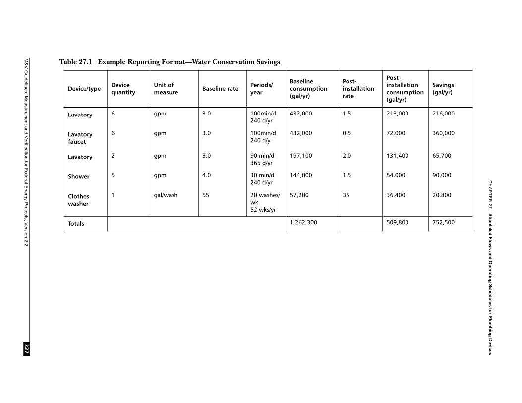
M&
V G
uidelines: Measurem
ent and Verification for F
ederal Energy P
rojects, Version 2.2
CH
AP
TE
R 2
7S
tipu
lated F
low
s and
Op
erating
Sch
edu
les for P
lum
bin
g D
evices
227
tion
Post-installation consumption (gal/yr)
Savings(gal/yr)
213,000 216,000
72,000 360,000
131,400 65,700
54,000 90,000
36,400 20,800
509,800 752,500
Table 27.1 Example Reporting Format—Water Conservation Savings
Device/typeDevice quantity
Unit of measure
Baseline ratePeriods/year
Baseline consumption (gal/yr)
Post-installarate
Lavatory 6 gpm 3.0 100min/d240 d/yr
432,000 1.5
Lavatory faucet
6 gpm 3.0 100min/d240 d/y
432,000 0.5
Lavatory 2 gpm 3.0 90 min/d365 d/yr
197,100 2.0
Shower 5 gpm 4.0 30 min/d240 d/yr
144,000 1.5
Clothes washer
1 gal/wash 55 20 washes/wk52 wks/yr
57,200 35
Totals 1,262,300

28Methods:
WCM-A-02
Metered Flows and Stipulated or MeteredDurations for Plumbing Devices
28.1 WCM Definition
Many water conservation projects focus simply on replacing existing plumbing devices (the baseline) with new devices. The new devices are designed to deliver water at low flow rates or low consumption per cycle during consistent operating schedules. Designs limit the flow and/or cycle consumption to fixed maximumvalues, usually stated in the product specifications. Other projects simply involve the changing of water consumption schedules.
For these projects, the operating schedules are known and consistent. Typicalapplications include water closet, urinal, irrigation head and shower headconversions, and irrigation schedule changes.
This M&V method is appropriate only for water conservation projects in which, for baseline and post-installation conditions, the following apply:
• Device flow rates and/or water consumption per cycle can be measured for each applicable water-consuming device (or group of devices).
• Device usage can be determined from short-term monitoring or from othersurveys or research on typical units, because usage patterns are known or can be estimated with reasonable accuracy and operating schedules are consistent from one time period to the next.
28.2 Overview of Verification Method
Method WCM-A-02 assumes that the federal agency and the ESCO are confident that unit water consumption can be defined, measured, and stipulated for each device type, and that operating cycles (flushes, hours of use, or another parameter) can be quantified and stipulated.
Surveys are required to document existing (baseline) and new (post-installation) devices (sprinklers, toilets, etc.) and characteristics. The surveys should include the following information in a set format, preferably in a matrix that allows each device type to be listed by location:
M&V Guidelines: Measurement and Verification for Federal Energy Projects, Version 2.2228
CHAPTER 28 Metered Flows and Stipulated or Metered Durations for Plumbing Devices
• Generic type of device
• Location
• Number of devices (of the same type and flow) counted in each location
• Unit of measure for each device group (gpm flow, gallons per flush, etc.)
• Period of service in consistent units (hours per day, flushes per day, etc.)
• Water consumption per unit of measure, existing devices (base case)
• Water consumption per unit of measure, new devices.
Even though this method, in comparison to method WCM-A-01, requires measure-ment or metering of water flow for each type of water-consuming device, it is a good idea to conduct a “reality check” of the assumptions for consumption and savings against the facility's total, or, if available, sub-meter; billing data.
Existing devices are subject to many variables and usually will not display a flowrating; thus, this method can provide reliable data if metering is done correctly. Modern water conservation devices are usually rated by the manufacturers; however, published data should generally not be used for the documentation of a newinstallation. Comparison with measurements of existing conditions is required.
Flow measurements can be made either with flow meters or by volumetric means. Suitable flow meters are selected for appropriate accuracy, and they have flow ratings that conform to field conditions. Flow rates can also be determined by measuring how much water (i.e., its volume) is used or discharged during a measured time interval. For example, water discharged from a faucet is collected for a timed period of 2 minutes, and when measured is found to be exactly 5 gallons; the flow rate is 5 gallons divided by 2 minutes, or 2.5 gpm). Volumetric measurements are usually used to determine how much water is discharged during a set cycle, such as one flush of a water closet. Dishwashers and clothes washers also have set cycles, although care must be taken to recognize possible variations, such as water-saver cycles or extra rinse cycles.
Spot measurements are useful not only to quantify water consumption but also to make sure specific devices are assigned to appropriate device groups, and to verify that all devices assigned to the group have similar performance characteristics.
Savings estimates also require good estimates of how frequently each type of device is used or for how long it operates per day, week, or year. Frequency information may need to be determined by measuring how often each type of device is used, most likely by sample counts. Any surveys of this type must account for variables in user practices, such as shower duration, double-flushing of water closets, and the amount of rinsing that occurs during food preparation. Given these variables, it is often pref-erable to use results from published surveys that are representative of the actual field conditions, or use short-term metering to determine patterns during representative time periods.
Water consumption savings are based on the following:
M&V Guidelines: Measurement and Verification for Federal Energy Projects, Version 2.2 229
SECTION VII M&V for Water Projects
• Measured baseline consumption for each type of device
• Measured post-installation consumption for each type of device (includingpossibly using manufacturers' flow measurements that are stipulated for use, assuming approval by the agency and ESCO)
• Number of devices, both baseline and post-installation, of each type
• Measured or stipulated cycles or hours per year for each operating scenario, both baseline and post-installation.
28.3 Calculation of Savings in Water Consumption and Demand
28.3.1 Baseline Water ConsumptionThe baseline conditions identified in the pre-installation equipment survey will be defined either by the federal agency or the ESCO. If the baseline is defined by the federal agency, the ESCO will have an opportunity to verify the baseline. If thebaseline is defined by the ESCO, the federal agency will verify the baseline.
Steps involved in establishing the baseline water consumption are as follows:
• Conduct a pre-installation facility survey
• Determine flow rates of representative existing devices.
In the pre-installation survey, all devices to be changed are inventoried. Devicelocations and corresponding facility drawings should be included with the survey submittal. The surveys will include, in a set format, device types, number of devices of each type, locations, units of measure for each device group, periods of service, and water consumption per unit of measure.
28.3.2 Adjustments to Baseline Water ConsumptionAfter WCM installation, adjustments to baseline water consumption may be required because of factors such as remodeling or changes in occupancy. Methods for making adjustments should be specified in the site-specific M&V plan.
28.3.3 Post-Installation Water ConsumptionThe new equipment will be defined and surveyed by the ESCO and verified by the federal agency.
After new devices are installed, spot metering may again be necessary, using theprocedures that were used for the baseline devices, and entering results in astandard survey form. See part 28.3.1. In some instances, the manufacturer's water consumption values for the new devices can be used; however, if there is any doubt about the water consumption figures supplied by the manufacturer, metering should be used. In either case, installation of the new devices should be field verified.
M&V Guidelines: Measurement and Verification for Federal Energy Projects, Version 2.2230
CHAPTER 28 Metered Flows and Stipulated or Metered Durations for Plumbing Devices
28.3.4 Operating Hours/CyclesInformation about device usage must be captured during the pre-installation facility survey. Usage factors must be consistent with the units of measurement applied to each device type, so that the product of the flow rate or cycle flow times the usagefactor will determine the total consumption for the time period. Examples:
1. A shower has a flow rate expressed in gpm; determine how many minutes the shower is used each year (or how many minutes per day and the number of active days each year).
2. A tank-type toilet discharges a certain number of gallons per flush; determine how many times it is flushed each year (or how many times each day and the number of active days each year).
Once defined, the operating hours will be stipulated—i.e., agreed to by the federal agency and the ESCO. Sources of stipulated hours can be any of the following:
• Pre-metering of representative devices by the ESCO or federal agency
• Research reports or documents provided by vendors or third parties
• Results from other projects in similar facilities
• Operator logs or documented schedules from building management systems (infrequent).
Operating periods or cycles can be estimated for each individual device or for groups of devices with similar applications and schedules. Each group type should have similar use patterns and comparable average operating hours. These areexamples of such groupings:
• Kitchen sink usage in all two-bedroom apartments within a residential complex
• All top-load clothes washers (of the same rated load capacity) within alaundromat.
Note that baseline and post-installation total operating hours may differ.
See Appendix D for information on sampling.
M&V Guidelines: Measurement and Verification for Federal Energy Projects, Version 2.2 231

SECTION VII M&V for Water Projects
28.4 Calculating Water Consumption Savings
The following is an example of water savings calculation using method WCM-A-02.
Table 28.1 is a summary of sample baseline and post-installation water consumption measurements and savings calculations using the above equations.
28.5 Method Specific Issues for the M&V Plan
Specific M&V issues that may need to be addressed in the site-specific M&V plans and that are related to this M&V method include the following:
• Defining operating scenarios for the devices affected by the WCM.
• Providing a source and documentation for any consumption and operating cycle assumptions for each scenario, for baseline and post-installation case.
• Stipulating a meter specification and spot metering methodology, includingcalibration methods.
• Providing a source of any consumption and operating-cycle assumptions used in developing baseline and post-installation assumptions.
Example: Calculating water savings using WCM-A-02
.A tank-type toilet is measured to consume 3 gpf and is used on average 20 times a day (based on a facility survey) throughout the year; the annual water consumption is:
3 x 20 x 365 = 21,900 gallons per year
If the toilet is replaced with one that is measured to consume 1.6 gpf, and the usage is unchanged, the post-installation annual water consumption is
1.6 x 20 x 365 = 11,680 gallons per year
And the savings in water consumption is
21,900 - 11,680 = 10,220 gallons per year
M&V Guidelines: Measurement and Verification for Federal Energy Projects, Version 2.2232
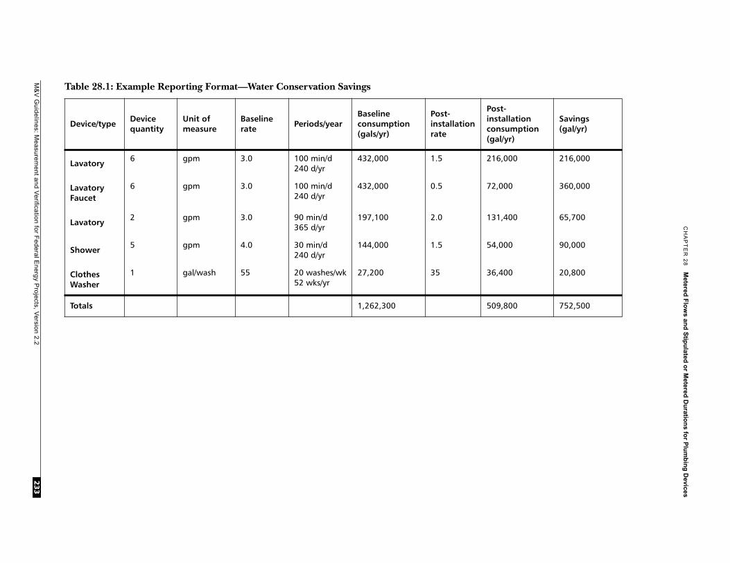
CH
AP
TE
R 2
8M
etered F
low
s and
Stip
ulated
or M
etered D
uratio
ns fo
r Plu
mb
ing
Devices
M&
V G
uidelines: Measurem
ent and Verification for F
ederal Energy P
rojects, Version 2.2
233
Ta
Dlation mption r)
Savings (gal/yr)
La00 216,000
LaFa
0 360,000
La00 65,700
S0 90,000
CW
0 20,800
To 00 752,500
ble 28.1: Example Reporting Format—Water Conservation Savings
evice/typeDevicequantity
Unit of measure
Baselinerate
Periods/yearBaseline consumption (gals/yr)
Post-installation rate
Post-instalconsu(gal/y
vatory6 gpm 3.0 100 min/d
240 d/yr432,000 1.5 216,0
vatoryucet
6 gpm 3.0 100 min/d240 d/yr
432,000 0.5 72,00
vatory2 gpm 3.0 90 min/d
365 d/yr197,100 2.0 131,4
hower5 gpm 4.0 30 min/d
240 d/yr144,000 1.5 54,00
lothes asher
1 gal/wash 55 20 washes/wk52 wks/yr
27,200 35 36,40
tals 1,262,300 509,8
29Methods:
WCM-B-01
All Water Uses Compatible with Sub-Meteringor Monitoring
29.1 WCM Definition
Some water conservation projects can easily be sub-metered, and others are complex or large enough that the added cost of sub-metering is justified. Sub-metering isindicated when the water-consuming devices do not have constant flows, water usage patterns are expected to change or vary unpredictably, operating schedules are erratic (and can be known only through monitoring), and/or metering costs are small in comparison to other project costs. Sub-metering, if done properly, often provides very useful information and the most accurate savings estimates.
Typical applications include retrofits that are done only in a portion of a very large building, multibuilding developments, irrigation projects, and certain HVACsystems, especially those with evaporative cooling.
This M&V method is appropriate only for water conservation projects in which, for the baseline and post-installation conditions, the following apply:
• Water flowing to most of the water conservation project, or all of it, can be, or is, measured by sub-metering at one or more points.
• Periods of measurement, for the baseline and post-installation, can be defined for comparable seasons and/or regular usage patterns.
29.2 Overview of Verification Method
Method WCM-B-01 assumes that the federal agency and the ESCO agree to usemeasured flows of supply water as the basis for evaluating the savings from a water conservation project, including impacts of any leaks, occupancy changes, or other effects that may be reflected in the measured values.
Water flowing to or through for any group of devices is likely to change over a period of time. Periodic or continuous monitoring of the project with sub-metering will help identify sudden changes—e.g., the onset of leaks or the lax irrigation practices of gardeners. Ongoing metering improves the chances of maintaining full savings from the project, and perhaps increasing savings beyond expectations by usinginformation feedback.
M&V Guidelines: Measurement and Verification for Federal Energy Projects, Version 2.2234

CHAPTER 29 All Water Uses Compatible with Sub-Metering or Monitoring
Surveys are required to document existing (baseline) and new (post-installation) devices (sprinkler heads, toilets, etc.). Surveys should include the followinginformation in a set format, preferably in a matrix that allows each device typeto be listed by location:
• Generic type of water delivery device
• Location
• Number of devices (of the same type and flow) in each location
• Unit of measure for each device group (gpm flow, gpf, etc.)
• Period of service in consistent units (hours per day, flushes per day, etc.)
• Water consumption per unit of measure, existing devices (base case)
• Predicted water consumption per unit of measure, new devices.
The number of devices will normally be determined by device counts during field observations. In instances in which construction modules have been repeated and construction drawings or other documents show the complete installation, device counts may be extrapolated from counts in representative modules.
Water consumption savings are based on the following:
• Measured baseline consumption for the project
• Measured post-installation consumption for the project
• Metering and/or analysis of independent variables that affect baseline andpost-installation water-use.
Although this method requires metering water flow from individual devices or groups of devices, “reality checking” results against utility bills is still recommended.
29.3 Calculating Savings in Water Consumption and Demand
29.3.1 Baseline Water ConsumptionThe baseline conditions identified in the pre-installation equipment survey will be defined by either the federal agency or the ESCO. If the baseline is defined by the federal agency, the ESCO will have an opportunity to verify the baseline. If thebaseline is defined by the ESCO, the federal agency will verify the baseline.
Steps involved in establishing the baseline water consumption are as follows:
• Conduct a pre-installation facility survey
• Determine flow rates by sub-metering
• Document the independent variables that affect baseline water-use (e.g., weather or occupancy).
M&V Guidelines: Measurement and Verification for Federal Energy Projects, Version 2.2 235
SECTION VII M&V for Water Projects
Pre-Installation Facility SurveyIn the pre-installation survey, all devices to be changed are inventoried. Devicelocations and corresponding facility drawings should be included with the survey submittal. The surveys will include, in a set format, device types, and number of devices of each type, locations, units of measure for each device group, periods of service, and estimated water consumption per unit of measure.
Flow Determination By Sub-meteringSub-metered data must be collected and recorded for the water conservation project. If meter readings are taken at more than one independent location, waterconsumption for the same periods should be added together. Results may need to be interpolated or extrapolated if meter locations do not coincide exactly with water flows within the project boundaries. Readings must encompass a period long enough to average normal fluctuations in water-use (e.g., daily and weekly patterns of use).
In some facilities, water-use may change seasonally (e.g., rainy and dry seasons), so separate data will be needed for each season.
29.3.2 Adjustments to Baseline Water ConsumptionAfter WCM installation, adjustments to baseline water consumption may be required because of factors such as remodeling or changes in occupancy. Methods for making adjustments should be specified in the site-specific M&V plan.
29.3.3 Post-Installation Water ConsumptionThe new equipment will be defined and surveyed by the ESCO and verified by the federal agency.
After new devices are installed, installation and proper operation of the new devices should be field-verified. Sub-metered water consumption measurements should be repeated at the same metering points and for periods of measurement that are either (a) continuous or (b) for each year of the agreement, comparable to those used in the pre-installation measurements.
29.3.4 Operating Hours/CyclesInformation about water consumption patterns must be captured during the pre-installation facility survey. At a minimum, the record should define the types of water consumption devices and how many units of each type are in active use. Additional data collection is encouraged for how intensively the equipment is used and hours of service. This information provides the means to confirm that metered data aremeeting expectations. It also provides a comparative record, should consumption patterns change. An adjustment will be needed if baseline and post-installationoperating conditions differ.
M&V Guidelines: Measurement and Verification for Federal Energy Projects, Version 2.2236
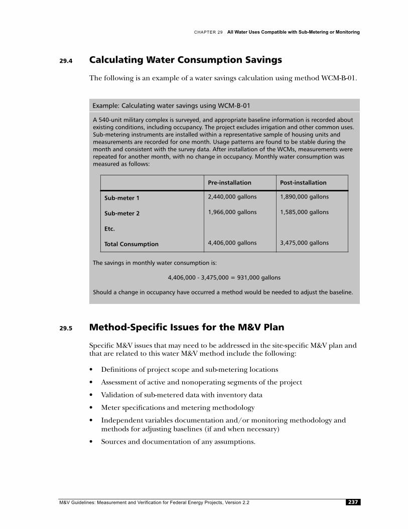
CHAPTER 29 All Water Uses Compatible with Sub-Metering or Monitoring
29.4 Calculating Water Consumption Savings
The following is an example of a water savings calculation using method WCM-B-01.
29.5 Method-Specific Issues for the M&V Plan
Specific M&V issues that may need to be addressed in the site-specific M&V plan and that are related to this water M&V method include the following:
• Definitions of project scope and sub-metering locations
• Assessment of active and nonoperating segments of the project
• Validation of sub-metered data with inventory data
• Meter specifications and metering methodology
• Independent variables documentation and/or monitoring methodology and methods for adjusting baselines (if and when necessary)
• Sources and documentation of any assumptions.
Example: Calculating water savings using WCM-B-01
A 540-unit military complex is surveyed, and appropriate baseline information is recorded about existing conditions, including occupancy. The project excludes irrigation and other common uses. Sub-metering instruments are installed within a representative sample of housing units andmeasurements are recorded for one month. Usage patterns are found to be stable during the month and consistent with the survey data. After installation of the WCMs, measurements were repeated for another month, with no change in occupancy. Monthly water consumption was measured as follows:
The savings in monthly water consumption is:
4,406,000 - 3,475,000 = 931,000 gallons
Should a change in occupancy have occurred a method would be needed to adjust the baseline.
Pre-installation Post-installation
Sub-meter 1 2,440,000 gallons 1,890,000 gallons
Sub-meter 2 1,966,000 gallons 1,585,000 gallons
Etc.
Total Consumption 4,406,000 gallons 3,475,000 gallons
M&V Guidelines: Measurement and Verification for Federal Energy Projects, Version 2.2 237

30Methods:
WCM-C-01
All Water Uses Compatible withWhole-Facility Metering
30.1 WCM Definition
Measurement and verification for some water conservation projects can best be achieved with whole-facility metering, usually with the servicing utility's own water supply meter. All end-use technologies can be verified with Option C, provided that the reduction in consumption is larger than the associated modeling error—i.e., the savings are not “lost in the noise.” This option may be used in cases where there is a high degree of interaction between different water conservation measures, and/or it is difficult to measure individual component savings. Accounting for changes is the major challenge associated with Option C, particularly for long-term contracts.
“Whole-building” metering may include several buildings or an entire complex. Whole-building metering is appropriate when (a) water-consuming devices do not have constant flows, and (b) the use of splintering is not practical or is prohibitively expensive. Compared with methods relying on stipulated values or spot measure-ments, whole-building metering may provide superior information and improve the accuracy of the savings estimates. Typical applications include large scale plumbing fixture retrofits and irrigation projects.
This M&V method is appropriate when the following apply:
• The utility meter (or other whole-building meter) can measure water flowing to most or all of the water conservation project.
• Periods of measurement, for the baseline and post-installation, can be defined for comparable seasons and/or other usage patterns.
• Project water savings are at least 20% of the water consumption recorded by the whole-facility meter.
30.2 Overview of Verification Method
Method WCM-C-01 assumes that the federal agency and the ESCO agree to use whole-facility measured-supply water flows as the basis for evaluating savings from a water conservation project, including impacts of any leaks, occupancy changes, or other effects which may be reflected in the measured values.
M&V Guidelines: Measurement and Verification for Federal Energy Projects, Version 2.2238

CHAPTER 30 All Water Uses Compatible with Whole-Facility Metering
Water demand in any project is likely to change over time. Periodic or continuous monitoring of the project with whole-building metering will help identify changes, such as the onset of leaks or lax irrigation practices of gardeners. Ongoing metering improves the opportunity for maintaining full savings from the project, and perhaps increasing the savings beyond expectations using information feedback. However, whole-facility metering does not help pinpoint changes as well as sub-metering does.
Surveys are required to document existing (baseline) and new (post-installation) devices. Surveys should include the following information in a set format, preferably in a matrix that allows each device type to be listed by location:
• Generic type of water delivery device
• Location
• Number of devices (of the same type and flow) in each location
• Unit of measure for each device group (gpm flow, gpf, etc.)
• Period of service in consistent units (hours per day, flushes per day, etc.)
• Water consumption per unit of measure, existing devices (base case)
• Predicted water consumption per unit of measure, new devices.
This method does not require measurements or metering of water flow fromindividual devices or other water-delivery devices; however, “reality checking” results requires reasonable estimates of unit water consumption, number of devices, and frequency of use. Flows recorded with metering should be consistent with theseestimates, within appropriate allowances. The number of devices will normally be determined by device counts during field observations. In instances whereconstruction modules have been repeated and construction drawings or otherdocuments show the complete installation, device counts may be extrapolated from counts in representative modules.
Readings must be taken and recorded regularly, either monthly or at a morefrequent interval. Recording meters that provide electronic data (with telemetry) may be very valuable tools.
Water consumption savings are based on the following:
• Measured baseline consumption for the project
• Measured post-installation consumption for the project
• Metering and/or analysis of independent variables that effect baseline andpost-installation energy use.
M&V Guidelines: Measurement and Verification for Federal Energy Projects, Version 2.2 239

SECTION VII M&V for Water Projects
30.3 Calculating Savings in Water Consumption and Demand
30.3.1 Baseline Water ConsumptionThe baseline conditions identified in the pre-installation equipment survey will be defined either by the federal agency or by the ESCO. If the baseline is defined by the federal agency, the ESCO will have an opportunity to verify the baseline. If thebaseline is defined by the ESCO, the federal agency will verify the baseline.
Steps involved in establishing the baseline water consumption are as follows:
• Conduct a pre-installation facility survey
• Determine flow rates by whole-building metering
• Document the independent variables that affect baseline water-use(e.g., occupancy and weather).
Pre-Installation Facility SurveyIn the pre-installation survey, an inventory is made of all plumbing devices and other water-consuming devices to be changed. Device locations and the corresponding facility drawing should be included with the survey submittal. The surveys will include, in a set format, device types and number of devices of each type, locations, units of measure for each device group, periods of service, and estimated waterconsumption per unit of measure. This information is required primarily in case any baseline adjustments are required during the term of the agreement.
Flow Determination by Whole-Building MeteringMetered data must be collected and recorded for the water conservation project. Results may need to be interpolated or extrapolated if meter locations do notcoincide exactly with water flows within project boundaries. Readings must be taken for a period long enough to average out normal fluctuations in water use (e.g., daily and weekly patterns of use).
In some facilities, water use may change seasonally (e.g., rainy and dry seasons), so separate data will be needed for each season.
When readings are taken by the utility, they will often be for periods a little longer or shorter than one month; such readings should be adjusted in proportion to the number of days included in the reading interval, to reflect corrected values for exactly one month at a time.
Documentation of Independent VariablesA regression analysis is required to properly estimate savings using whole-facility analysis. To complete the analysis, data on independent variables that affect water use need to be collected throughout the term of the agreement and for the baseline. Whole-facility, or billing, analysis is discussed in Chapter 21.
M&V Guidelines: Measurement and Verification for Federal Energy Projects, Version 2.2240
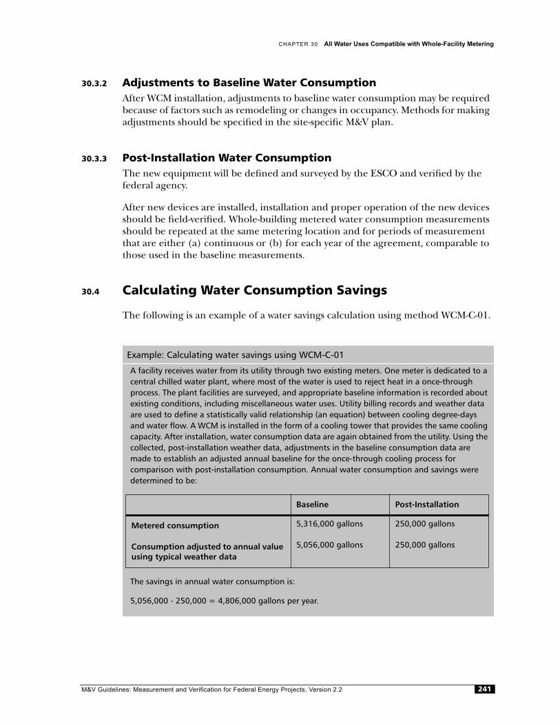
CHAPTER 30 All Water Uses Compatible with Whole-Facility Metering
30.3.2 Adjustments to Baseline Water ConsumptionAfter WCM installation, adjustments to baseline water consumption may be required because of factors such as remodeling or changes in occupancy. Methods for making adjustments should be specified in the site-specific M&V plan.
30.3.3 Post-Installation Water ConsumptionThe new equipment will be defined and surveyed by the ESCO and verified by the federal agency.
After new devices are installed, installation and proper operation of the new devices should be field-verified. Whole-building metered water consumption measurements should be repeated at the same metering location and for periods of measurement that are either (a) continuous or (b) for each year of the agreement, comparable to those used in the baseline measurements.
30.4 Calculating Water Consumption Savings
The following is an example of a water savings calculation using method WCM-C-01.
Example: Calculating water savings using WCM-C-01
A facility receives water from its utility through two existing meters. One meter is dedicated to a central chilled water plant, where most of the water is used to reject heat in a once-throughprocess. The plant facilities are surveyed, and appropriate baseline information is recorded about existing conditions, including miscellaneous water uses. Utility billing records and weather data are used to define a statistically valid relationship (an equation) between cooling degree-days and water flow. A WCM is installed in the form of a cooling tower that provides the same cooling capacity. After installation, water consumption data are again obtained from the utility. Using the collected, post-installation weather data, adjustments in the baseline consumption data are made to establish an adjusted annual baseline for the once-through cooling process forcomparison with post-installation consumption. Annual water consumption and savings were determined to be:
The savings in annual water consumption is:
5,056,000 - 250,000 = 4,806,000 gallons per year.
Baseline Post-Installation
Metered consumption 5,316,000 gallons 250,000 gallons
Consumption adjusted to annual value using typical weather data
5,056,000 gallons 250,000 gallons
M&V Guidelines: Measurement and Verification for Federal Energy Projects, Version 2.2 241

SECTION VII M&V for Water Projects
30.5 Method-Specific Issues for the M&V Plan
M&V issues that need to be addressed in a site-specific M&V plan and that are related to this M&V method include the following:
• Definitions of project scope and sub-metering locations
• Validation (reality check) of meter water consumption data with inventory data
• Meter specifications and metering methodology
• Documentation and/or monitoring methodology for independent variables and methods for adjusting baselines (if and when necessary)
• Criteria for determining acceptable accuracy in analysis equations, e.g, minimum R2 values for regression models
• Sources and documentation of any assumptions concerning variables used in analysis equations.
M&V Guidelines: Measurement and Verification for Federal Energy Projects, Version 2.2242
31Methods:
WCM-D-01
Calibrated Simulation Analysis ofWater-Consuming Systems
31.1 WCM Definition
Modeling, or computerized simulation, techniques are used for measurement and verification when impacts of WCMs are too complex to analyze cost-effectively with Option B, when the savings are too small to show up in whole-facility meter analysis (Option C), or when Option A methods cannot provide the level of detail oraccuracy required.
Few computer-based modeling tools have been developed to analyze waterconservation measures. Those that are available are not as sophisticated or widelyvalidated as their building-energy-simulation counterparts. More sophisticatedengineering simulation tools have been developed for complex water problems such as network flow, but they are generally not suitable for analyzing water conservation measures. The relative lack of water conservation modeling tools may be attributed partly to a slower start for efforts in the water conservation field; but the primaryconsideration is that most water conservation projects are generally not complex, and formal computational tools generally are not needed. Thus, most projects should take advantage of Option A, B, or C.
Option D may be appropriate when the water project is unusually complex, when existing metering is not congruent with the project, and/or when long-termsub-metering would be too difficult or costly to implement. Applications might include WCMs involving evaporative cooling systems or irrigation projects using moisture sensors.
31.2 Overview of Verification Method
Computer simulations and other modeling techniques that are used to predict water consumption and demand are generally recognized as being more of an art form than an exact science. The reason for this view is that water-use in a building or other development can depend on a large number of factors, many of which are difficult to predict or are beyond the control of project managers, and are thus hard to“program” into a model. Factors include the unique behaviors of individuals who use the facilities.
M&V Guidelines: Measurement and Verification for Federal Energy Projects, Version 2.2 243

SECTION VII M&V for Water Projects
A key element of this method is calibrating the model with (a) utility metering data and/or (b) short-term or spot metering of individual devices or systems. In some facilities, the utilization factor may change seasonally (e.g., dry versus rainy season), and appropriate data will be needed for each season. If the simulation results do not agree with measured data, often only trained and experience personnel are able to determine the cause of the discrepancy and correct the model.
Comparative data are required to document existing (baseline) and new (post-installation) characteristics. Data may be available in the form of inventories and engineering documents (drawings, specifications). These data should be reflected in the model's input parameters; however, it is not sufficient that there is a change in simulated water flow or consumption. Even if there is agreement that additional documentation is not needed for the project as a whole, a suitable sampling plan is still required in which first-hand observations are made both before and after the WCM, to confirm that the physical changes have in fact been made.
It is usually helpful to summarize the following information and present it in a set format, preferably in a matrix that allows each device type to be listed by location:
• Generic type of device or other water delivery device
• Location
• Number of devices (of the same type and flow) in each location
• Unit of measure for each device group (gpm flow, gpf, etc.)
• Period of service in consistent units (hours per day, flushes per day, etc.)
• Water consumption per unit of measure, existing devices (base case)
• Water consumption per unit of measure, new devices.
Water consumption savings are based on the following:
• Simulated baseline consumption for the project
• Simulated post-installation consumption for the project
• Analysis of the effects of independent variables in order to determine anynecessary baseline adjustments.
31.3 Calculating Savings in Water Consumption and Demand
31.3.1 Baseline Water ConsumptionThe baseline conditions identified in the pre-installation equipment survey will be defined either by the federal agency or by the ESCO. If the baseline is defined by the federal agency, the ESCO will have the opportunity to verify the baseline. If thebaseline is defined by the ESCO, the federal agency will verify the baseline. Steps involved in determining the baseline water consumption are as follows:
M&V Guidelines: Measurement and Verification for Federal Energy Projects, Version 2.2244

CHAPTER 31 Calibrated Simulation Analysis of Water-Consuming Systems
• Conduct a pre-installation facility survey or sampling
• Perform modeling to compute the consumption
• Collect metering data to calibrate the model
• Document the independent variables that affect baseline water-use.
Pre-Installation Facility SurveyIn the pre-installation survey, an inventory is made of all plumbing devices and other water-consuming devices to be changed. Device locations and corresponding facility drawings should be included with the survey submittal. The surveys will include, in a set format, device types and the number of devices of each type, locations, units of measure for each device group, periods of service, and estimated water consumption per unit of measure.
Modeling and CalibrationMeasurement and verification of WCMs using computer simulation or othermodeling approaches involves the following steps:
• Select appropriate simulation software or other computational basis.
• Conduct detailed site surveys, collecting water-related building and equipment data.
• Select appropriate program inputs such as weather, occupancy schedules, and irrigation schedules.
• Select appropriate calibration data, usually from utility billings or sub-metering.
• Input baseline data into the model; simulate the baseline conditions.
• Calibrate the baseline model.
• Input WCM specifications and simulate the post-installation conditions.
• Estimate energy-savings by comparing the water consumption predicted by the baseline and post-installation models.
More information on calibrated simulation can be found in Chapter 24.
31.3.2 Adjustments to Baseline Water ConsumptionAfter WCM installation, adjustments to baseline water consumption may be required because of factors such as remodeling or changes in occupancy. Methods for making adjustments should be specified in the site-specific M&V plan.
31.3.3 Post-Installation Water ConsumptionThe new equipment will be defined and surveyed by the ESCO and verified by the federal agency. Installation of the new devices and proper operation should befield-verified. Unless field changes are observed, the previously modeled post-installation consumption figures may be accepted without change.
M&V Guidelines: Measurement and Verification for Federal Energy Projects, Version 2.2 245
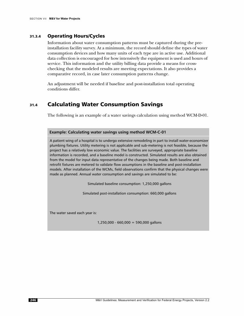
SECTION VII M&V for Water Projects
31.3.4 Operating Hours/CyclesInformation about water consumption patterns must be captured during the pre-installation facility survey. At a minimum, the record should define the types of water consumption devices and how many units of each type are in active use. Additional data collection is encouraged for how intensively the equipment is used and hours of service. This information and the utility billing data provide a means for cross-checking that the modeled results are meeting expectations. It also provides acomparative record, in case later consumption patterns change.
An adjustment will be needed if baseline and post-installation total operatingconditions differ.
31.4 Calculating Water Consumption Savings
The following is an example of a water savings calculation using method WCM-D-01.
Example: Calculating water savings using method WCM-C-01
A patient wing of a hospital is to undergo extensive remodeling in part to install water-economizer plumbing fixtures. Utility metering is not applicable and sub-metering is not feasible, because the project has a relatively low economic value. The facilities are surveyed, appropriate baselineinformation is recorded, and a baseline model is constructed. Simulated results are also obtained from the model for input data representative of the changes being made. Both baseline andretrofit fixtures are metered to validate flow assumptions in the baseline and post-installation models. After installation of the WCMs, field observations confirm that the physical changes were made as planned. Annual water consumption and savings are simulated to be:
Simulated baseline consumption: 1,250,000 gallons
Simulated post-installation consumption: 660,000 gallons
The water saved each year is:
1,250,000 - 660,000 = 590,000 gallons
M&V Guidelines: Measurement and Verification for Federal Energy Projects, Version 2.2246

CHAPTER 31 Calibrated Simulation Analysis of Water-Consuming Systems
31.5 Method-Specific Issues for the M&V Plan
M&V issues that need to be addressed in the site-specific M&V plan and that are related to this water M&V method include the following:
• Definitions of project scope and submetering locations
• Definition of models to be used, who will conduct the modeling, how the models will be calibrated, what the criteria will be for establishing calibration, and the documentation of the models that will be provided
• Documentation and/or monitoring methodology for independent variables and methods for adjusting baselines (if and when necessary)
• Sources and documentation of any assumptions to be used in models.
M&V Guidelines: Measurement and Verification for Federal Energy Projects, Version 2.2 247

M&V Guidelines:
Section VIII:M&V Plan Overviews for Other
Project Categories
This section includes information on M&V methods for federal perfor-mance contracts that involve projects other than conventional waterconservation and/or energy-efficiency opportunities.
Chapter Project Description Method Number
32 New construction projects NC-A-01NC-B-01NC-C-01NC-C-02NC-D-01
33 Operations and maintenance mea-sures
OM-01
34 Cogeneration projects COG-01
35 Renewable energy projects REN-01
Measurement and Verification for Federal Energy Projects, Version 2.2 249
32Methods:
NC-A-01NC-B-01NC-C-01NC-C-02NC-D-01
New Construction Projects
32.1 Introduction
Construction of new buildings represents an opportunity to achieve energy savings through performance contracting. Capital budgets are usually limited for newbuilding projects and consequently many energy conservation measures, which may require more capital for equipment purchase or more integrated (and costly) design, are not included. The result can be a significant and unnecessary increase in a building’s operating cost and more importantly, a lost opportunity to obtain cost-effective energy savings over the typical 50-year life of a building.
Performance-based contracts may be used to produce energy-efficient buildings. The ESCO's involvement in a new construction project may range from providing single ECMs to providing multiple, interacting ECMs or providing fully integrated building designs.
32.2 Project Definition
The projects covered by these verification plans include any ECM in new construc-tion that can be reasonably modeled with accepted engineering practices. Such projects may include lighting, motors, controls, and HVAC. The projects may be as simple as replacing lighting fixtures with more efficient fixtures or as complex as the integrated design of ECMs in the building architecture.
Project definition in new construction is critical, as the “baseline” building only exists in concept, not in physical reality. The baseline energy performance is obtained from a model of the baseline building. Depending on the complexity of the project, the building may be modeled by calculations in a simple spreadsheet or by a thorough description of the complete building in a whole-building computer simula-tionanalysis.
In addition, the installed ECMs in the energy-efficient building, as in any retrofit project, must be verified. In new construction, projects verification may be simple inspection and spot checking and/or metering of lighting or motor ECMs, or through well-documented commissioning processes for complex ECMs, such as HVAC or controls systems.
M&V Guidelines: Measurement and Verification for Federal Energy Projects, Version 2.2250

CHAPTER 32 New Construction Projects
32.3 Overview Of New Construction M&V Options
32.3.1 GeneralIn all new construction M&V options, the energy performance of the baseline must meet current building energy codes and standards. For federal agencies, the Energy Policy Act of 1992 requires that new non-residential buildings must meet or exceed ASHRAE Building Energy Efficiency Standard 90.1. In most situations this standard will be used to define the baseline. Defining 90.1 is not necessarily straightforward or easy. All energy savings estimates are obtained from comparison with this baseline.
This section presents five new construction M&V options, which are similar inconcept to the retrofit M&V options:
• Option NC-A-01: Stipulated baseline and savings, verified equipmentperformance.
• Option NC-B-01: Stipulated baseline, savings based on verified equipmentperformance and estimating tool using short-or long-term measurements
• Option NC-C-01: Whole-building baseline simulation, savings based on differ-ence with actual billing data, verified ECM performance
• Option NC-C-02: Stipulated baseline, savings based on comparison with similar buildings with and without ECMs
• Option NC-D-01: Calibrated whole-building simulation of as-built building,baseline performance defined by “ECM Subtraction Technique,” verified ECM performance.
32.3.2 Steps Common to All M&V OptionsThe basic steps in new construction M&V are similar to those in retrofit M&V. These steps are as follows:1
1. Define the Baseline. Baseline definition is a two-part process. First, a designbaseline must be developed. This can be the stipulation of specific baseline equipment or specifying whole-building compliance with energy codes orstandards. Once the design baseline has been established, analytical tools are used to estimate the associated energy performance of the baseline.
2. Define Energy-Efficient Design and Projected Savings. The energy-efficient design is defined through the building design process and is the natural final outcome of that process. Analytical tools are used to estimate performance of the energy-efficient design. First year estimated savings are determined by subtraction of energy efficient design use from baseline use. The estimation process should also include the identification and quantification of factors which could affect the
1. The steps are similar to those defined in the International Performance Measurement and Verification Protocol (IPMVP), 1997.
M&V Guidelines: Measurement and Verification for Federal Energy Projects, Version 2.2 251
SECTION VII I M&V Plan Overviews for Other Project Categories
performance of both the baseline and energy-efficient design, and how thesefactors will impact energy performance.
3. Define General M&V Approach. This chapter presents new building M&V methods that are roughly analogous to the M&V retrofit Options A, B, C, and D, which are presented earlier in this guideline. Options A and B are directed at end-usemeasures, and Options C and D address whole-building M&V methods. Therelative suitability of each approach is a function of:
– The M&V objectives and the requirements of any related performancecontracts.
– The number of ECMs and the degree of interaction with each other as well as with other systems.
– The technical practicality and issues associated with M&V of particular ECMs or broader whole-building ECMs and strategies.
– Current trends toward more integrated and holistic new building designs, which are moving M&V requirements more to the whole-building methods.
The definition of the general M&V approach should also include adescription of how savings will be determined. This section should include the equations that determine energy and demand savings and the conditions under which the equations are used. The assumptions made in developing the data used in the equations should be described as well. Any supporting calculations that are made to manipulate the data (e.g., statistical sampling of lighting fixture operating hours, determining plug load densities) must be documented.
4. Prepare Project-Specific M&V Plan. Development of an M&V plan should begin during the design phase of the project. It should include the definition of the baseline building, the definition of the energy-efficient building, and adescription of how the ECMs will be verified, what data will be collected, what analytical tools will be used, how savings will be determined (including equa-tions), and what annual activities will be performed and reported.
The project-specific M&V plan also describes the scope of the project and all issues pertaining to savings determination. These issues are listed in part 32.5. Starting the M&V plan development early in the process forces the development of commissioning plans and O&M procedures for ECMs where necessary.Commissioning and O&M procedures are in the ESCOs interest to ensuresavings are realized over the course of the project.
5. Verify Installation and Commissioning of ECMs or Energy-Efficient Strategies. Installation and proper operation is verified through site inspections and spot measurements as necessary, combined with review of commissioning reports, fluid balancing reports, etc. Any deviations should be noted and addressed when determining the performance of the energy-efficient building.
M&V Guidelines: Measurement and Verification for Federal Energy Projects, Version 2.2252
CHAPTER 32 New Construction Projects
6. Determine Savings Under Actual Post-Installation Conditions. Virtually all energy performance projections are predicated upon certain assumptions regarding operational conditions, such as occupancy and weather. This affects both the baseline and energy-efficient design estimations. Deviations from the operational assumptions must be tracked by an appropriate mechanism (i.e., a site survey, short-and/or long-term metering) and the baseline and energy-efficientprojections modified accordingly to determine actual savings.
7. Re-Evaluate at Appropriate Intervals. Ongoing performance of ECMs or energy-efficient strategies and the associated energy savings must be re-evaluated and verified at intervals and over a time frame appropriate to M&V and relatedperformance contract requirements. This also allows ongoing management and correction of significant deviations from projected performance.
32.3.3 Description of New Construction M&V Options
Method NC-A-01: Stipulated baseline and savings, verified equipment performance This method is suitable for projects where the potential to perform needs to beverified, but actual savings can be stipulated using estimations of baselineperformance and ECM performance based on the verified as-built performance potential. Note that while ECM performance potential must be physically verified (through one-time and/or periodic verification), the savings stipulation is made using assumed typical operating conditions for both the baseline and energy-efficient estimations. Also note that this is a modification of the initial performance estimations that supported the decision to implement the ECM. It is not sufficient to simply use the initial estimates “as-is” without performance potential verification.
Although the most rudimentary of M&V methods, NC-A-01 is adequate for manypurposes, including performance contracts. It can be applied to essentially any end-use ECM—motors, lighting ballasts, chillers—and is particularly well suited to constant or predictable loads. The method of verification of performance potential depends on the measure savings uncertainty, the confidence level required, thepracticality of physical performance measurement, and M&V costs. The method can range from physical inspection and verification of nameplate data to short-term metering. The following table illustrates the advantages and disadvantages of this method.
Advantages Disadvantages
• Simplicity
• Low cost
• Reasonable accuracy with constant or predictable loads
• Diminished accuracy with non-constant or unpredictable loads
M&V Guidelines: Measurement and Verification for Federal Energy Projects, Version 2.2 253
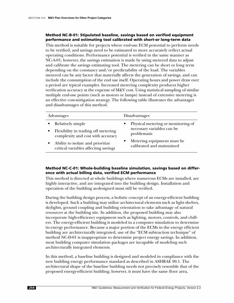
SECTION VII I M&V Plan Overviews for Other Project Categories
Method NC-B-01: Stipulated baseline, savings based on verified equipment performance and estimating tool calibrated with short-or long-term dataThis method is suitable for projects where end-use ECM potential to perform needs to be verified, and savings need to be estimated to more accurately reflect actual operating conditions. Performance potential is verified in the same manner asNC-A-01; however, the savings estimation is made by using metered data to adjust and calibrate the savings estimating tool. The metering can be short or long term depending on the constancy and/or predictability of the load. The variables metered can be any factor that materially affects the generation of savings, and can include the consumption of the end use itself. Operating hours and power draw over a period are typical examples. Increased metering complexity produces higherverification accuracy at the expense of M&V cost. Using statistical sampling of similar multiple end-use points (such as motors or lamps) instead of extensive metering is an effective cost-mitigation strategy. The following table illustrates the advantages and disadvantages of this method.
Method NC-C-01: Whole-building baseline simulation, savings based on differ-ence with actual billing data, verified ECM performance This method is directed at whole buildings where numerous ECMs are installed, are highly interactive, and are integrated into the building design. Installation andoperation of the building as-designed must still be verified.
During the building design process, a holistic concept of an energy-efficient building is developed. Such a building may utilize architectural elements such as light shelves, skylights, ground coupling and building orientation to take advantage of natural resources at the building site. In addition, the proposed building may alsoincorporate high-efficiency equipment such as lighting, motors, controls, and chill-ers. The energy-efficient building is modeled in a computer simulation to determine its energy performance. Because a major portion of the ECMs in the energy efficient building are architecturally integrated, use of the “ECM subtraction technique” of method NC-D-01 is inappropriate to determine project energy savings. In addition, most building computer simulation packages are incapable of modeling sucharchitecturally integrated elements.
In this method, a baseline building is designed and modeled in compliance with the new building energy performance standard as described in ASHRAE 90.1. Thearchitectural shape of the baseline building needs not precisely resemble that of the proposed energy-efficient building; however, it must have the same floor area,
Advantages Disadvantages
• Relatively simple
• Flexibility in trading off metering complexity and cost with accuracy
• Ability to isolate and prioritizecritical variables affecting savings
• Physical metering or monitoring of necessary variables can beproblematic
• Metering equipment must becalibrated and maintained
M&V Guidelines: Measurement and Verification for Federal Energy Projects, Version 2.2254
CHAPTER 32 New Construction Projects
similar surface-area-to-volume ratio, support the same occupancy, comfort andbuilding operation schedule requirements, and any other system function required by the federal agency for the new building.
In most cases, the estimating tool will be an hourly computer energy simulationpackage. The baseline building is stipulated and modeled in the design process. Actual operating conditions of the as-built building that materially impact energy use are monitored and/or metered throughout the M&V term. These conditions include, at a minimum:
• Weather data
• Occupancy - density and schedule
• HVAC run time and set points
• Lighting schedules
• Plug load power density and schedules.
The baseline simulation model is adjusted and re-run under actual operatingconditions for a given period. The resulting adjusted baseline performance iscompared to the actual utility billing meter data for the same period to generate the savings. Since there is no real data to check the baseline building model, the baseline model should be reviewed by an independent, qualified third party who is familiar with both ASHRAE standard 90.1 and building simulation modelling. A supplemen-tary quality control reference for the baseline is to compare it with the utility data of similar buildings.
Aside from adjusting simulation models to reflect actual operating conditions, the single greatest factor affecting the accuracy of this method is the quality of computer modeling and simulations. Most hourly simulation programs tend to underestimate actual energy use due to factors such as precise default equipment sizing (i.e., no over-sizing to accommodate equipment increments or safety factors), broad HVAC zoning (due either to zone handling limitations in the software or user lack ofattention to detail), and HVAC air volume sizing based solely on thermodynamic requirements. The following table lists the advantages and disadvantages of this method.
M&V Guidelines: Measurement and Verification for Federal Energy Projects, Version 2.2 255
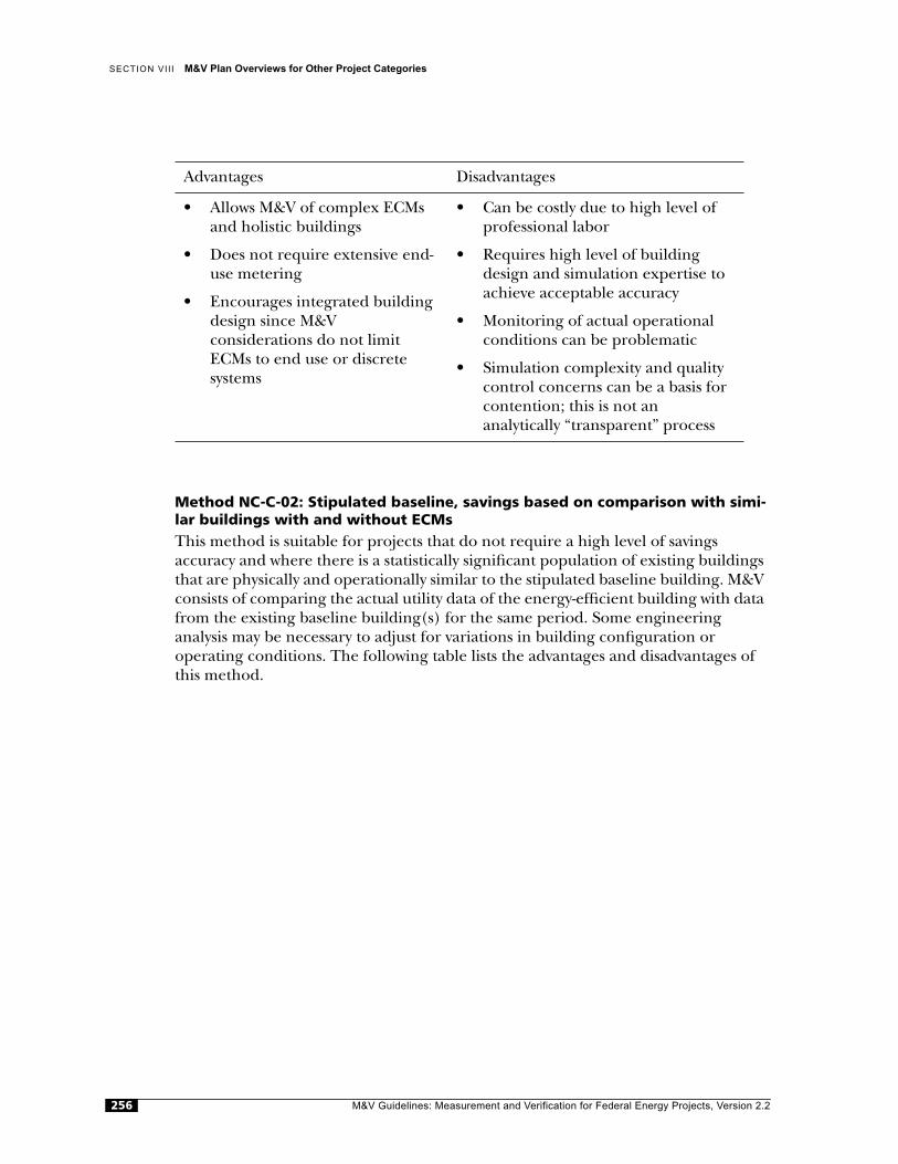
SECTION VII I M&V Plan Overviews for Other Project Categories
Method NC-C-02: Stipulated baseline, savings based on comparison with simi-lar buildings with and without ECMs This method is suitable for projects that do not require a high level of savingsaccuracy and where there is a statistically significant population of existing buildings that are physically and operationally similar to the stipulated baseline building. M&V consists of comparing the actual utility data of the energy-efficient building with data from the existing baseline building(s) for the same period. Some engineeringanalysis may be necessary to adjust for variations in building configuration oroperating conditions. The following table lists the advantages and disadvantages of this method.
Advantages Disadvantages
• Allows M&V of complex ECMs and holistic buildings
• Does not require extensive end-use metering
• Encourages integrated building design since M&Vconsiderations do not limit ECMs to end use or discretesystems
• Can be costly due to high level of professional labor
• Requires high level of building design and simulation expertise to achieve acceptable accuracy
• Monitoring of actual operational conditions can be problematic
• Simulation complexity and quality control concerns can be a basis for contention; this is not ananalytically “transparent” process
M&V Guidelines: Measurement and Verification for Federal Energy Projects, Version 2.2256

CHAPTER 32 New Construction Projects
Method NC-D-01: Calibrated whole-building simulation of as-built building, baseline performance defined by “ECM Subtraction Technique,” verified ECM performanceThis method is directed at buildings where numerous, highly interactive ECMs will be installed, rendering savings estimations of individual ECMs impractical orinappropriate. ECM installation and operation must still be verified. This method is not appropriate for buildings which derive energy efficiency from integrated, holistic building designs. The appropriate method for holistic building designs is method NC-C-01.
During the building design process, the baseline building and energy-efficientbuilding are defined. Energy-efficient lighting, motors, controls, chillers, boilers, and so on that would not be included in the baseline building may be included as part of the proposed energy-efficient building; however, the baseline building must perform to current federal building energy performance standards, which is ASHRAE 90.1.
The energy performance of the baseline building and the energy-efficient buildingis determined by estimation through computer simulation. In most cases, theestimating tool will be a quality hourly computer simulation program. First year energy and cost savings are estimated during the design process. Verification of the ECMs is achieved through commissioning. Variables that impact the as-builtbuilding's energy consumption are monitored beginning in the first year.
Advantages Disadvantages
• Relatively simple and low cost
• Limits technical contentious-ness (if method is mutually agreeable in concept)
• May be difficult to find reliable and statistically meaningful baselinecomparison buildings
• Securing the cooperation of baseline building owners/managers can be problematic
• Variability in operation, mainte-nance, etc., between baseline and energy-efficient building(s) limits accuracy of the method
• Accuracy issues limit the method to energy-efficient buildings with ECMs or performance strategies that are expected to generate significantsavings; the anticipated savings must substantially exceed the accuracytolerances of the comparisons
M&V Guidelines: Measurement and Verification for Federal Energy Projects, Version 2.2 257
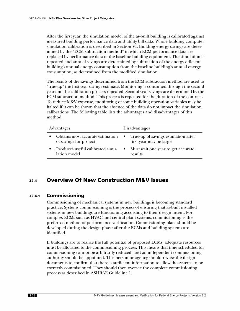
SECTION VII I M&V Plan Overviews for Other Project Categories
After the first year, the simulation model of the as-built building is calibrated against measured building performance data and utility bill data. Whole building computer simulation calibration is described in Section VI. Building energy savings are deter-mined by the “ECM subtraction method” in which ECM performance data are replaced by performance data of the baseline building equipment. The simulation is repeated and annual savings are determined by subtraction of the energy efficient building's annual energy consumption from the baseline building's annual energy consumption, as determined from the modified simulation.
The results of the savings determined from the ECM subtraction method are used to “true-up” the first year savings estimate. Monitoring is continued through the second year and the calibration process repeated. Second year savings are determined by the ECM subtraction method. This process is repeated for the duration of the contract. To reduce M&V expense, monitoring of some building operation variables may be halted if it can be shown that the absence of the data do not impact the simulation calibrations. The following table lists the advantages and disadvantages of this method.
32.4 Overview Of New Construction M&V Issues
32.4.1 Commissioning Commissioning of mechanical systems in new buildings is becoming standardpractice. Systems commissioning is the process of ensuring that as-built installedsystems in new buildings are functioning according to their design intent. Forcomplex ECMs such as HVAC and central plant systems, commissioning is thepreferred method of performance verification. Commissioning plans should be developed during the design phase after the ECMs and building systems areidentified.
If buildings are to realize the full potential of proposed ECMs, adequate resources must be allocated to the commissioning process. This means that time scheduled for commissioning cannot be arbitrarily reduced, and an independent commissioning authority should be appointed. This person or agency should review the designdocuments to confirm that there is sufficient information to allow the systems to be correctly commissioned. They should then oversee the complete commissioningprocess as described in ASHRAE Guideline 1.
Advantages Disadvantages
• Obtains most accurate estimation of savings for project
• Produces useful calibrated simu-lation model
• True-up of savings estimation after first year may be large
• Must wait one year to get accurate results
M&V Guidelines: Measurement and Verification for Federal Energy Projects, Version 2.2258

CHAPTER 32 New Construction Projects
Some ECMs, such as natural ventilation, daylighting, nighttime flushing, and use of building thermal mass, result in a building that behaves differently than does aconventional building. It is important that the commissioning contractor, thebuilding maintenance staff, and the occupants understand how the building works.
In addition to performing building commissioning, the design intent and correct operation of ECMs should be documented for the building maintenance staff. The ESCO may even consider conducting training sessions for the staff to further ensure that the ECMs will be properly maintained and operated.
StandardsThe suggested minimum standards to be used are as follows:
• NEBB Procedural Standards for Testing, Adjusting, Balancing of Environmental Systems, Vienna, VA: National Environmental Balancing Bureau, 1983.
• AABC National Standards 1982, Washington, DC: Associated Air BalanceCouncil, 1982.
• ASHRAE G-1 Guideline for Commissioning of HVAC Systems, Atlanta: American Society of Heating, Refrigerating, and Air-Conditioning Engineers, Inc., 1989.
• ANSI/ASHRAE 111, Practices for Measurement, Testing, Adjusting andBalancing of Building Heating, Ventilation, Air-Conditioning, and Refrigerating Systems, Atlanta: American Society of Heating, Refrigerating, andAir-Conditioning Engineers, Inc., 1988.
• In addition to recommendations in the above Standards, the Commissioning Authority as defined in ASHRAE G-1 must be independent of the installingcontractor.
DDC CommissioningNearly all buildings today (aside from very small ones) have some form of directdigital controls (DDC). While procedures for checking valve stroke and operation, location, and calibration of sensors are well documented, there is less clarity oncommissioning and verification of the software functions and sequence ofoperations. It is not the intention of the guidelines to define a commissioningprocedure for DDC systems. It is vitally important that the system is correctlycommissioned especially if the system is to be used for verifying energy performance. True system verification requires each point and sequence of operation to be checked. For a large and complex building, this may involve two controls engineers for approximately four weeks.
Documenting the ProcessDocumentation of the commissioning process becomes critical for performancecontracting. Clear documentation of all setpoints and air and water quantities as well as any deviations from the design documents will form an essential part of thepost-installation verification process. Both the commissioning agent and theperformance verification agent need to review the proposed documentation before commissioning starts. This should ensure that the level of information presented in completed documents is adequate for the performance verification method selected.
M&V Guidelines: Measurement and Verification for Federal Energy Projects, Version 2.2 259
SECTION VII I M&V Plan Overviews for Other Project Categories
32.4.2 Using Actual Versus Typical Operating ConditionsWhenever a new building's energy performance is to be compared with an estimate of performance calculated during design, real building performance or input to the calculation has to be modified so that the two can be compared. Even if the new building is being compared to other typical buildings, local climate, occupancy, internal load, etc. must be noted. Some major parameters affecting energy use in real buildings are discussed below.
WeatherMost computer simulations used for estimating energy use typical annual weather data for input. If relevant data are recorded at the building, then the computed energy can be modified to account for actual annual weather conditions. It isimportant that the actual data recorded matches the input requirements of thecomputer analysis. For instance, if the program uses hourly weather data, hourly data should be recorded. And if the program uses solar insulation data, this information needs to be measured (a solar pyranometer would not normally be specified for a building control system).
Lighting Actual lighting load may vary significantly from the lighting-use profile assumed in the computer analysis. Metering the overall power load will not give a true indication of lighting use profiles. If lighting circuits are metered, a better indication can be obtained. For buildings that feature extensive daylighting schemes, the metering of lighting circuits needs to be broken down to fairly small zones so that predicted reductions in lighting energy can be checked against actual use. Monitoring a large number of lighting circuits can be expensive. Alternate methods are to monitortypical circuits on each facade of the building and some interior zones.
Small PowerThe issues for small power measurement are similar to those for lighting. Ideally each panel board should be monitored; however, monitoring a representativesample may be sufficient. The practice of estimating cooling loads based on the nameplate rating of computing equipment has led to over-designed systems. Real measurements of power consumption of office equipment over time would be avaluable resource for HVAC system designers. If monitoring of actual powerconsumption is not available, an actual count of in-use equipment can be made. A few spot measurements of power draw can then be used to estimate the diversityfactor to be applied to the equipment ratings.
OccupancyOccupancy loads are the most difficult building loads to compare. Most computer analysis programs assume a uniform distribution of people throughout the building. In actual buildings, however, neither the total number nor the location of people remain static. The computer analysis assumes an occupancy profile for the building, but in the case of a multi-tenant building, real occupancy profiles may vary signifi-cantly from floor to floor. A practical solution to estimating real occupancy profiles is to observe actual occupancy on a few representative days each year, and use these data to extrapolate annual occupancy patterns.
M&V Guidelines: Measurement and Verification for Federal Energy Projects, Version 2.2260
CHAPTER 32 New Construction Projects
Internal TemperaturesInternal temperature set points are often varied by facility staff in response tooccupant complaints. Actual set points must be recorded so that meaningfulcomparisons can be made with predictions. This information should be available from the energy management system.
User-Controlled BuildingsNaturally ventilated buildings and mixed-mode buildings (combination of natural ventilation and air-conditioning) pose a difficult problem for comparing predicted versus actual operating conditions. These buildings often have high occupantsatisfaction due to the fact that occupants have some control over their environment. Tracking these effects is difficult, and is most accurately achieved through EMS or other system sensors.
32.4.3 Computer Simulation Model Issues All methods (with the exception of NC-C-02) rely on “estimating tools” to generate the necessary baseline and energy efficient performance projections. These tools are presumed to be computer-based and can range in sophistication from spreadsheets programmed using engineering calculation methodologies to hourly whole-building simulations. The level of sophistication should be appropriate for the complexity of the ECMs, the M&V method used, and the necessary degree of accuracy orconfidence. Tools used in a performance contract context should not only bemutually agreeable to the parties, but should also be technically comprehensible to all concerned. In this regard, more demanding analyses (such as hourly simulations) should be conducted using one of the more widely recognized and validatedpackages.
Computer SimulationThe accuracy of computer simulations is an issue that has been the subject ofconsiderable debate in all building engineering sectors. The reality is that most mainstream hourly computer simulation programs tend to underestimate actual energy usage, particularly when applied by less experienced users. Some of the main reasons are:
• Default or automatic HVAC plant and large secondary equipment sizing is usually “right on” the load, with perhaps some provision for a user-specified safety factor. In reality, available equipment capacity increments, load pickup considerations, and redundancy/backup considerations result in considerably larger as-builtsystems and equipment than the software defaults for auto-sizing.
• HVAC air supply volumes are usually defaulted or auto-sized based only onthermodynamic load. In real practice, air volume required to meet the pureheating or cooling load is usually a fraction of what is normally considerednecessary for adequate air circulation in the space. Consequently, default or auto-sizing of air supply volumes inevitably results in a considerably undersized air system in the simulation. This can result in catastrophic underestimation of energy use if a constant volume (CV) reheat-based system is being evaluated.
M&V Guidelines: Measurement and Verification for Federal Energy Projects, Version 2.2 261
SECTION VII I M&V Plan Overviews for Other Project Categories
• The default HVAC configurations and control sequences for ventilation in many programs simply presume an exact specified ventilation rate to the space. This approach may not consider the practicalities of central air-handling design that drive up the overall building ventilation rate. The result, again, is significant underestimation of energy use in CV reheat-based systems.
• Broad-block HVAC zoning in all simulations results in the mixing and canceling of local heating and cooling loads, which are normally met individually in aproperly zoned real-world HVAC system. The result is an energy useunderestimation. In this regard, it is a general axiom that the more tightly and accurately the HVAC zoning is modeled, the more accurate the simulation results.
• A related HVAC zoning issue is the “corner office effect.” This occurs when areal-world chronic problem zone (such as a corner office or boardroom) isconsolidated into a larger simulation zone. The high chronic load is “diluted,” and sometimes effectively neutralized. This is a serious problem in the simulation of supply air reset strategies. Since the simulation does not “see” a chronic high load area, the supply air reset modulates through a much wider range than would be the real-world case. This results in underestimation of design flow rates,system reheat, and plant energy demand.
The knowledge and experience of the simulation engineer and the rigor of thesimulation model are paramount to result accuracy. All of the issues listed above can be avoided, but a thorough understanding of building design principles, withparticular emphasis on HVAC design and operation is required. Simulation “short-cuts” and program defaults should only be used if there is a clear understanding of their implications.
In many cases, it is impossible to model all ECMs with a single estimating tool. In these instances it is acceptable to use a number of estimating approaches andconsolidate the results in a single final result. Many simulation programs haveprovisions for manual input to override certain operational variables or factors. Many stock system models or components can be programmed to mimic a non-stock configuration or operational sequence. The latter should only be attempted by the most experienced users.
32.4.4 Use of Energy Management Systems or Data Loggers for Data Collection and AnalysisThe building EMS can provide much of the monitoring necessary for the verification process; however, the system and software requirements need to be specified so that the EMS can be a useful tool for verification as well as its primary function ofcontrolling building systems.
There may be parameters that need monitoring for verification, but are not required for control. These points must be specified in the design documents. Electric power metering is an example. Trending of small power, lighting and main feed powerconsumption may be very useful for high quality verification.
M&V Guidelines: Measurement and Verification for Federal Energy Projects, Version 2.2262
CHAPTER 32 New Construction Projects
Other functions that can easily be incorporated into the software are automatic recording of changes in set-points. The evaluation team can have a direct read-only connection into the EMS via a modem link. This allows all the trending data to be analyzed and collated by the evaluation team in their office. It is not unusual for many of the trending capabilities required for verification to be incorporated in an EMS. All too often, however, the building facility staff is not properly trained in the use of the system and is unaware of the many additional monitoring and diagnostic capabilities of the system.
32.4.5 Changes in Building Operation and ECMs During Termof Performance ContractUnder a performance contract, all changes in operation, from system on-times to control set-points, must be recorded. Methods for estimating what effect these changes have must be agreed upon, preferably at the start of the contract. Changes in the system due to ECMs can be addressed using the methods already developed for existing buildings. In addition, there may also be changes in set-points during the first year to optimize the performance of the systems. These changes are part of the commissioning process of the original ECMs and so do not require a separateanalysis.
Buildings with high turnover rates and changes of occupancy present a significant workload in recording and re-evaluation of energy performance. In many cases these changes may have a significant effect on the building energy consumption; there-fore, the method for recording and incorporating them into the verification method must be defined.
32.5 Site-Specific M&V Plans
Issues that need to be addressed in the project-specific M&V plan and that are related to new construction projects include:
• Which analytical tool will be used to calculate savings from ECMs. If the tool is an hourly building simulation package, it should be one of the generally accepted hourly simulation packages, such as DOE2 or BLAST. Also provide the version number, the supplier of the program, and what, if any, pre- and post-processors will be used
• A thorough baseline description must be provided. The scale of this description should be on the order of the scale of the project. Additionally, documentation of how the baseline building meets ASHRAE standard 90.1 must be provided. It should be clear how the energy performance of the baseline building will be obtained.
• Description of post-retrofit building which includes identification of the ECMs to be installed, and how the energy performance of the ECMs will be obtained.
M&V Guidelines: Measurement and Verification for Federal Energy Projects, Version 2.2 263

SECTION VII I M&V Plan Overviews for Other Project Categories
• Description of any building operation conditions (i.e., set-points, schedules) that will be used to predict the baseline and energy-efficient building energyperformance.
• Documentation of the ECM or building modeling strategy and projectprocedure, including how the building models will be calibrated or adjusted with actual measurements or utility bill data.
• Identification of spot and short-term measurements to be made
• Description of commissioning procedures for complex ECMs and relatedoperations manuals to be developed, as necessary.
• For calibrated computer simulation of the new building, documentation of the calibration procedure as specified in Section VI.
M&V Guidelines: Measurement and Verification for Federal Energy Projects, Version 2.2264
33Methods:
OM-01
Operations and Maintenance Measures
This chapter is a “place-holder” for discussing some of the issues associated with M&V of O&M measures. Future efforts by FEMP to develop M&V methods and test them on a range of projects will result in M&V methods for O&M projects being defined in future editions of this document. In the meantime, it is hoped that material in this chapter will help federal agency project managers and procurement officers develop O&M projects and understand the M&V issues that need to be addressed.
33.1 Project Definition
Federal agencies are allowed to use ESPC for installation of O&M measures that can demonstrably reduce facility energy costs and related O&M expenses. Specifically Regulation Section § 8287c. defines the term “energy savings” as a reduction in the cost of energy, from a base cost established through a methodology set forth in the contract, utilized in an existing federally owned building or buildings or other federally owned facilities as a result of:
1. The lease or purchase of operating equipment, improvements, altered operation and maintenance (O&M), or technical services; or
2. The increased efficient use of existing energy sources by cogeneration or heatrecovery, excluding any cogeneration process for other than a federally owned building or buildings or other federally owned facilities.
O&M measures do not necessarily involve the installation of new equipment.They can include repairs of defective equipment or equipment that is not operating as efficiently as possible (e.g., broken HVAC economizer systems), commissioning, improvedmaintenance procedures (including computerized tracking systems), training, or the installation of computerized systems that monitor system performance and report warnings when systems are not operating properly. In some cases O&M measures can include the out-sourcing of facility O&M staffing.
Methods for measuring and verifying O&M project savings are not nearly as developed or tested as methods for the M&V of energy or water projects. As discussed below, there are several issues associated with the M&V of O&M projects that make quantifyingbaseline conditions, post-installation conditions, and savings very difficult.
M&V Guidelines: Measurement and Verification for Federal Energy Projects, Version 2.2 265
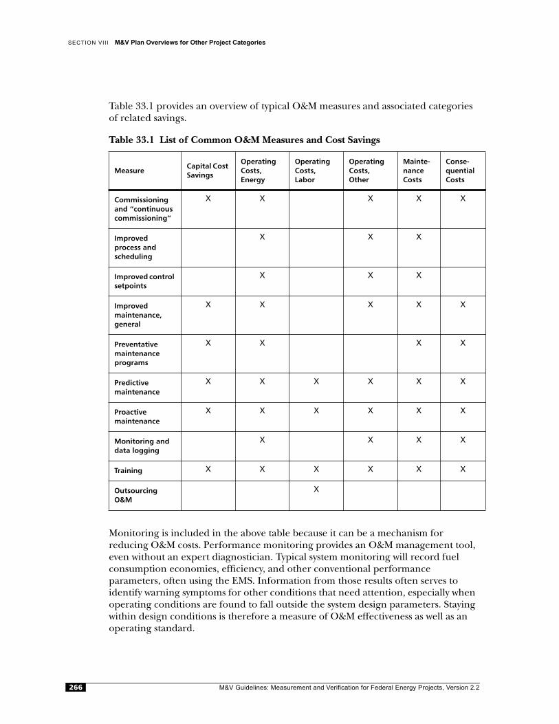
SECTION VII I M&V Plan Overviews for Other Project Categories
Table 33.1 provides an overview of typical O&M measures and associated categories of related savings.
Table 33.1 List of Common O&M Measures and Cost Savings
Monitoring is included in the above table because it can be a mechanism forreducing O&M costs. Performance monitoring provides an O&M management tool, even without an expert diagnostician. Typical system monitoring will record fuelconsumption economies, efficiency, and other conventional performanceparameters, often using the EMS. Information from those results often serves to identify warning symptoms for other conditions that need attention, especially when operating conditions are found to fall outside the system design parameters. Staying within design conditions is therefore a measure of O&M effectiveness as well as an operating standard.
MeasureCapital Cost Savings
Operating Costs, Energy
Operating Costs,Labor
Operating Costs,Other
Mainte-nance Costs
Conse-quential Costs
Commissioning and “continuous commissioning”
X X X X X
Improved process and scheduling
X X X
Improved control setpoints
X X X
Improved maintenance, general
X X X X X
Preventative maintenance programs
X X X X
Predictive maintenance
X X X X X X
Proactive maintenance
X X X X X X
Monitoring and data logging
X X X X
Training X X X X X X
Outsourcing O&M
X
M&V Guidelines: Measurement and Verification for Federal Energy Projects, Version 2.2266
CHAPTER 33 Operations and Maintenance Measures
33.2 Overview of Operations and Maintenance M&V Issues
The energy and non-energy savings from O&M measures are difficult to quantify because:
• O&M measures are usually not limited to new pieces of equipment whose impacts can be isolated and measured.
• Baseline O&M procedures and costs are difficult to quantify, particularly if the current O&M practices are resulting in sub-standard comfort, equipment lives, indoor air quality, etc.
• Valuation of O&M savings may require trade-offs between short-term and long-term benefits and thus may require a long period of evaluation to determine true net benefits.
• Valuation of O&M costs and savings may involve intangibles such as risk andquality of service.
The following is a discussion of some of the issues associated with quantifying thesavings from O&M measures.1 The issues are compiled into the following categories:
• Valuation of savings
• Determining and adjusting baselines
• Persistence of savings and time period for analysis
• O&M Measure's indirect effects
• Can O&M savings justify M&V/metering activities.
33.2.1 Valuation of Non-Energy Savings
Energy CostsMany energy cost issues for O&M projects are similar to those for energy-efficiency measures, such as calculating energy costs versus kWh, kW or therm savings; however, other issues such as the trade-off between energy and other non-energy benefits (e.g., comfort) can affect the valuation of the overall O&M project.
Labor CostsWhen a project involves reductions in facility staffing as a means of reducing costs, there are several M&V issues (beyond labor relations and equity issues). These M&V issues include defining the baseline cost, tasks and performance of the existinglabor force, defining how labor costs will be reduced by the project (and not justtransferred to another “accounting category”), and providing sufficient oversight to
1. This discussion is from “Measuring and Verifying Savings from Improvements in Operation and Maintenance of Energy-Consuming Systems in Commercial and Institutional Buildings,” Steven R. Schiller and Gale Corsen, Schiller Associates, prepared for Lawrence Berkeley National Laboratory and U.S. Department of Energy’s Rebuild America Program, April, 1998.
M&V Guidelines: Measurement and Verification for Federal Energy Projects, Version 2.2 267
SECTION VII I M&V Plan Overviews for Other Project Categories
ensure that the tasks and performance of the labor force's replacement are equal to or above the specified requirements.
Operating Versus Capital Costs SavingsO&M measures can affect both labor cost and capital cost accounting categories, sometimes in opposite directions. Therefore, the M&V process must consider all cost accounting categories that are affected by the O&M measures to ensure that alldebits and credits are properly accounted for and used in the calculation ofperformance.
Another related issue is calculating a potential difference in residual value at the end of the performance period—a concept related to salvage value. For example, an agency would probably rather have performing systems at the end of the contract period instead of systems that are at the end of their useful life.
33.2.2 Determining and Adjusting Baselines
Setting Baseline M&V ProceduresDetermining the baseline from which savings are calculated for O&M measures often requires evaluating what the existing standards of performance are for O&Mactivities. These existing standards are often not well documented and the baseline definition can thus involve identifying the incremental value of “more robust” O&M measures versus “well done, conventional” measures—both of which need to be defined for the calculation of savings. In addition, while the standard for acceptable practice may be defined for the facility, actual practice may be sub-standard. Thus, should the savings be based on the O&M standard or the actual O&M practices?
Adjusting BaselinesBaseline adjustments are one of the more difficult aspects of energy project M&V. Issues associated with energy project baseline adjustments, as discussed in Section I, should be reviewed. Some of the unique issues associated with O&M measures are:
• Adjusting labor costs, equipment repair costs, and equipment replacement schedules based on changes in the facility's operation (e.g., changes to longer life lamps paid for by the facility).
• Period of time for assuming existing baseline conditions (e.g., how long should the current, perhaps poor, maintenance procedures be assumed to have been continued in the absence of the O&M measure).
33.2.3 Persistence of Savings and Time Period for AnalysisA simple O&M measure such as cleaning filters may achieve substantial energysavings, but only so long as people continue the practice. Concerns aboutpersistence apply to a wide variety of maintenance and operational items.Experience tells us that, after certain procedural improvements are made, atendency to slip back into earlier practices can occur in which clogged filters are
M&V Guidelines: Measurement and Verification for Federal Energy Projects, Version 2.2268
CHAPTER 33 Operations and Maintenance Measures
continued in use, controls are no longer optimized, drive belts are slipping, and repairs are not made. It is easy to conclude that many O&M measures have short lives.
Another important characteristic of O&M measures is the inherent coupling of short-term and long-term effects. O&M budget cuts “today” do not result in long term savings if they lead to still higher O&M costs “tomorrow.”
Long-Term Versus Short-Term SavingsReducing O&M costs in the short term is relatively easy. It is reducing O&M costs, and related equipment costs, over the long term while maintaining necessaryperformance levels (e.g., comfort and safety) that is difficult. Thus, M&V of O&M measures will tend to be a lengthy process to ensure that long-term savings are not sacrificed to achieve short-term benefits. This involves evaluating the persistence of savings and life-cycle savings.
Time Period for Analysis of PerformanceSeveral issues arise out of the time period for analysis. A standard response would be that savings should be determined for the full term of the performance contract. If the contract term is relatively short, however, then certain O&M measure impacts might not be considered, whether these are beneficial (e.g., extended equipment life) or not (e.g., shortened equipment life). For longer term contracts, a related question is how long is it “fair” to attribute savings to a measure? For example, some measures might correct deficiencies, such as broken economizer systems, that would have been repaired at some point regardless of a performance-based contract.
33.2.4 O&M Measure's Indirect Effects
Performance StandardsAs part of an O&M project, it is important to set facility standards for short-term and long-term satisfactory operations (e.g., comfort, lighting levels, temperature ranges, and air quality.) For the M&V of an O&M measure, it is important to:
1. Define criteria, methods and matrix for evaluating if the facility's performance standards have been met.
2. Define how adjustments will be made if operating standards are currently below standard and will be brought up to standard by the implementation of the O&M measures—e.g., outside air levels are brought up from below standard to levels required by standards. Note that, in some cases, the existing performance will be above standard, such as 100% outside air when it is not required, and the O&M measures may reduce the performance, but not below the set standard.
Valuation of Indirect BenefitsOperating and maintenance practices can have an important bearing on anorganization's less tangible costs, such as work stoppages, occupant satisfaction,consequential liability and insurance costs, and other risk factors. Measures for O&M savings have the same potential. These costs are often difficult to identify and even more difficult to value, requiring probability estimates for unlikely but critical events.
M&V Guidelines: Measurement and Verification for Federal Energy Projects, Version 2.2 269

SECTION VII I M&V Plan Overviews for Other Project Categories
For example, what if an O&M measure simultaneously changes several factors such as energy, indoor air quality, and comfort; how are these effects accounted for,verified, and measured? What if multiple changes result in degradation of some factor as well as improvements in others—how is this accounted for?
33.2.5 Calculation of Savings and O&M M&V OptionsBefore defining a framework for calculating O&M savings, the following general points need to be made:
• Savings from O&M measures will typically fall into one or more of the following three categories: energy, labor, and equipment. A possible fourth category isin-directs, which (almost by definition) are difficult to measure.
• The baseline costs and performance period costs should be tracked with stan-dard accounting practices. A key is to make sure that all costs are accounted for, including all those which rise or fall, due to the O&M measures.
In general, the baseline labor and equipment costs can be determined by either:
• Use of a “control group” set of facilities, which are similar to the one(s) with the O&M measures, to determine what the O&M costs would have been in the absence of the measures; or
• Use of historical cost data, adjusted as needed to changing needs and uses of the facility (e.g., more operating hours or higher occupancy loads effect on HVAC system operating costs).
There may be a practical minimum threshold, or level of effort, that must beconducted for measuring and verifying the savings from any O&M project; however, this issue is the same as for energy efficiency projects. The level of M&V rigor is going to vary according to (a) the value of the project and its expected benefits and (b) the acceptable level of risk in achieving the benefits.
The following is a discussion of measurement and verification options for O&Mmeasures. They are described per the framework of Option A, B, C, and D (seeSection I of this document).
33.2.6 Option A for O&M MeasuresOption A is for projects in which confirming the potential to generate savings is the primary objective of the M&V activities—versus the other options, where actual savings are estimated based on actual operating conditions. Therefore, Option A involves determining savings by validating certain key performance criteria (such as the operation of a new O&M software program or repairs to outside air dampers) and stipulating other parameters (such as assumed reductions in labor hours). Payments could be subject to change based on periodic assessments of O&Mactivities.
M&V Guidelines: Measurement and Verification for Federal Energy Projects, Version 2.2270
CHAPTER 33 Operations and Maintenance Measures
Stipulation is the easiest and least expensive method of determining savings. It can also be the least accurate (compared to using long-term measured data) and istypically the method with the greatest uncertainty of determining actual savings. Option A includes procedures for verifying that baseline conditions have beenproperly defined and the O&M measures, procedures, and/or systems:
• That were to be initiated have been initiated
• Meet contract specifications in terms of factors such as quality of service
• Are operating and performing in accordance with contract specifications and are meeting all functional tests
• During the term of the contract, continue to meet contract specifications in terms of factors such as quality, operation, and functional performance.
An example of Option A would be for an economizer repair program. The M&V activities would consist of checking the existing condition of the economizers and verifying their repair. A systems model may be used to predict energy use with the economizers in their existing (broken) condition (the baseline) and with properly operating economizers (post-installation energy use). Then savings would bestipulated as the difference between the baseline and post-installation predictions. Then each year of the performance contract the economizers' proper operation would be checked and the savings (payments) would not be re-calculated unless the economizer is not working to specification. The estimated savings would not be adjusted with changes in the weather or operation of the building as a whole.
33.2.7 Option BOption B is for projects where long-term measurement of performance is desired. Under Option B, individual O&M measures or systems are continuously monitored to determine performance, and this measured performance is compared withbaseline values to determine savings. Option B methods provide long-term operating (persistence) data on the O&M measures, procedures, and/or systems. In some cases, these data can be used to improve or optimize the operation of the equipment on a real-time basis, thereby improving the benefit of the retrofit. Option B also relies on the direct measurement of affected end uses.
Option B methods involve the use of post-installation measurement of one or more variables. The use of periodic or long-term measurement accounts for operatingvariations and will more closely approximate actual energy savings than the use of stipulations as defined for Option A. For example, energy use, labor costs, and equipment costs might be tracked after measure implementation for actualcomparison with baseline values.
An example of Option B would be for an economizer repair program. The M&V activities would consist of checking the existing condition of the economizers and verifying their repair. Chiller, and related auxiliary energy consumption, would be metered before and after repair of the economizers. The pre-existing energy data and independent variable data would be used to establish a baseline model. Savings would be calculated each year as the difference between the baseline energy model
M&V Guidelines: Measurement and Verification for Federal Energy Projects, Version 2.2 271
SECTION VII I M&V Plan Overviews for Other Project Categories
and measured, post-implementation data. The savings would thus be adjusted with changes in the weather or operation of the building as a whole.
An issue with Option B (and C) is that there may be changes that affect post-installation energy, labor, or equipment costs that are not associated with the O&M measures and are beyond the contractor's control. For example, there may be an increase in square footage of conditioned space or an increase in facility operating hours. Therefore, and this can be very complex, data would need to be collected in order to derive correlations between each of the cost categories and key factors such as occupancy, hours of operation, weather, industrial production rates, etc. Thebaseline would be adjusted to account for these changes depending on which party assumes the risk for changes to each variable.
33.2.8 Option COption C involves determining savings by comparing total facility energy and/or O&M costs before and after implementation of the measures. This is a “bottom-line” approach where documented costs (e.g. from utility bills or a company's accounting/tracking system) are used to identify savings. Option C methods are useful when measuring interactions between systems is desired, when determining the impact of projects that cannot be measured directly, and when a direct connection between the M&V effort and “bottom-line” is desired.
An Option C example would be similar to the one for Option B; however, with Option C, the total costs before and after the out-sourcing would be compared in total versus the comparison of each individual cost category.
33.3 Site-Specific Measurement and Verification Plan
At this time, measurement and verification plans for O&M measures will need to be custom developed by the ESCO and the federal agency since there are no guideline M&V methods (as there are for water and energy measures). It is highly recom-mended that not only the definition of the measures and their projected savings be established early in the planning process, but also the M&V approach. This is because for all ESPC agreements, the savings must be determined on an annual basis and thus, O&M measures must be defined in a way that their benefits can bequantified. If the O&M measures do not lend themselves to straightforwardquantification of savings, the contract negotiations can be held up or there willbe significant disputes during the term of the agreement.
The site-specific measurement and verification approach may be pre-specified in the ESPC contract between the federal agency and ESCO and/or agreed to after the award of the project. In either case, prior to the federal agency's approval of project construction, the ESCO will need to submit a final M&V plan that addresses thefollowing elements:
• Describe the facility and the project; include information on how the project saves energy and/or provides non-energy benefits and what key variables effect the realization of savings. An accounting type spreadsheet should be prepared
M&V Guidelines: Measurement and Verification for Federal Energy Projects, Version 2.2272
CHAPTER 33 Operations and Maintenance Measures
which shows estimated baseline costs and projected performance period costs for categories such as: labor, materials, equipment replacement, energy, and demand. Each of these values will need to be verified (baseline) or determined during the pre- and post-installation M&V processes.
• Indicate how the federal agency's budget will directly be reduced by themplementation of the measure(s). All payments to ESCOs must come from demonstrable savings to the agency's budget.
• Define the baseline O&M performance standard. If this standard is better and more expensive than the existing standard, then document how the baseline O&M budget will be established and calculated.
• Define the minimum performance standards (indoor air, temperature ranges, lighting levels, safety requirements, etc.) that are currently in place and those required once the measure is in place. Determine how benefits (or losses)associated with improvements (or reductions) in performance standards will be allocated between parties. Indicate how compliance with performance standards will be verified during the term of the agreement and what will happen if they are not met.
• Indicate who will conduct the M&V activities and prepare the M&V analyses and documentation.
• Define the details of how calculations will be made and the assumptions that will be made about significant variables or unknowns. For instance, labor costinflation rates, labor hours per specific task, and equipment life times with and without the new O&M measure. Describe any stipulations that will be made and the source of data for the stipulations. Describe any maintenance/management software that may be used. Show how calculations of O&M savings will be used to determine payments to the ESCO.
• Specify what metering and data logging equipment will be used, who will provide the equipment, its accuracy and calibration procedures, and how data from the metering will be validated and reported, including formats. Electronicformatted data directly from a meter or data logger are usually required forany short- or long-term metering.
• Specify what additional management oversight logs will be maintained, the nature and frequency of entries, and interpretation that is to be assigned to the results. Examples include logging of equipment failures and frequencies,equipment down time, and complaints.
• Describe any sampling that will be used, why it is required, sample sizes,documentation on how sample sizes were selected, and information on howrandom sample points will be selected.
• Define the level of accuracy which should be achieved for at least the keycomponents if not for the entire analysis.
• Indicate how quality assurance will be maintained and repeatability confirmed. For instance, “The data being collected will be checked every month andprovided to the federal agency.”
• Indicate which reports will be prepared, what they will contain, and when they will be provided.
M&V Guidelines: Measurement and Verification for Federal Energy Projects, Version 2.2 273
34Methods:
COG-01
Cogeneration Projects
This chapter introduces methods for determining savings from cogeneration projects and discusses some associated issues. As the number of cogeneration projects implemented through federal ESPCs increases, FEMP may develop more detailed M&V methods for inclusion in future editions of this document. In the meantime, it is hoped that material in this chapter will help federal agency project managers develop cogeneration projects and understand the M&V issues that need to be addressed.
34.1 Measure Definition
Federal agencies are allowed to use ESPCs for installation of cogeneration projects that can demonstrably reduce facility energy costs and related O&M expenses.Specifically, Regulation Section § 8287c. defines the term “energy savings” as areduction in the cost of energy, from a base cost established through a methodology set forth in the contract, utilized in an existing federally owned building or buildings or other federally owned facilities as a result of:
1. The lease or purchase of operating equipment, improvements, altered operation and maintenance, or technical services; or
2. The increased efficient use of existing energy sources by cogeneration or heat recovery, excluding any cogeneration process for other than a federally owned building or buildings or other federally owned facilities.
Cogeneration is the simultaneous generation of both electricity and thermal energy. Typical systems include packaged, gas turbines, and reciprocating engines with heat-recovery systems that can provide steam, hot water, or even chilled water through the use of thermal input chillers.
Depending on the performance contract arrangement the ESCO may either(a) simply provide the agency with thermal and electrical energy, at a discount to the baseline costs, or (b) share the net benefits of the entire cogeneration system—i.e.,a shared savings contract. Net benefits would be equal electrical and thermal output value and lower capital costs, fuel costs, and incremental O&M costs.
M&V Guidelines: Measurement and Verification for Federal Energy Projects, Version 2.2274
CHAPTER 34 Cogeneration Projects
34.2 Overview of M&V Methods For Cogeneration Projects
Determining the electrical and thermal output of cogeneration systems is relatively straightforward because fuel input and electrical output can be measured simply with many commercially available meters. Measuring thermal output (steam, hot water, or chilled water) of cogeneration systems is also straightforward, although not necessarily inexpensive, using commercial steam meters, water flow meters, andtemperature transducers.
Determining the full impact of changes in utility and O&M costs can be morecomplex because the analysis should include allowances for interconnect safety, rate changes, standby charges, air-quality control requirements, and the need to reject excess heat; all of which the agency will need to account for if the ESCO does not have full operating responsibility under the performance contract.
For determining savings, two general approaches may be used:
1. “One-for-one replacement” calculation
2. Net benefits calculation.
34.2.1 One-for-One ReplacementThis concept assumes that energy (electrical and thermal) produced by the cogener-ation system, and used in the facility, displaces energy that would have been provided by an existing source. Savings calculations depend on the type of financialarrangement—whether the ESCO is selling discounted electrical and thermal energy or whether it is a shared savings arrangement. The most likely application for this one-for-one replacement approach is the discounted energy cost arrangement in which energy savings are equal to the useful production of the cogeneration system. With the one-for-one replacement concept, all one has to do is (1) measure the net amount of energy produced by the cogeneration system and used in the facility, and (2) calculate the net economic value of the energy produced compared to what has been replaced. With some projects the value of reduced O&M costs are included in the calculation of benefits.
34.2.2 Net Energy-Use AnalysisThe net energy-use analysis approach is similar to Option B or C for energy-effi-ciency projects. Energy and operating costs for the facility (e.g., utility-supplied gas and electricity, any energy sales to other sites, labor costs, insurance costs) arecompared before and after the cogeneration system is installed to estimate the net benefit provided by the cogeneration system. This approach is most common with the shared savings financial arrangement. This approach is more complicated because (a) baseline fuel and operations costs need to be quantified, and (b) O&M costs need to be quantified and it is often difficult to allocate costs between the base case, the cogeneration system, and the non-cogeneration systems after thecogeneration system is installed.
M&V Guidelines: Measurement and Verification for Federal Energy Projects, Version 2.2 275
SECTION VII I M&V Plan Overviews for Other Project Categories
34.3 Overview of Cogeneration M&V Issues
Several key issues for evaluating cogeneration projects are:
• Benefits to the facility are usually calculated based on the portion of the cogener-ation output (thermal and electrical) that is actually used by the facility, versus total production. Net useful energy production may not be as easy to isolate and measure as gross production. Consideration should be given to items such as amount of vented steam versus delivered steam, enthalpy values of the thermal output (e.g. steam) versus enthalpy values of the thermal stream returned to the cogeneration system (e.g. condensate), parasitic power losses, and heat and power sales to other parties (e.g. back to the utility). As a side note, somecontracts will have provisions for how much energy the facility has to take, as a minimum, which can affect actual payments to the ESCO.
• Determining the economic value of the energy provided by the cogenerationsystem requires information on the value of the energy—i.e., what it would cost to purchase the energy from the existing sources, such as the utility or from a boiler plant. On the electrical side of the equation, current rate schedules should be used and the parties should take into account all changes in customer charges, stand-by charges, and rate structures due to the installation of thecogeneration system. For the thermal side the current rate schedules need to be used for the displaced fuel (e.g., natural gas for boilers or electricity for chillers) and the efficiency of the baseline thermal systems needs to be determined (e.g., boiler, hot water generator, or chiller efficiency) in order to calculate the value of the displaced thermal energy (e.g., steam, hot water, or chilled water).
• Correct incremental O&M costs associated with the existing (baseline) systems and the new cogeneration project need to be defined and used in the analyses. This is true for both the net energy benefit analysis approach or the one-for-one replacement approach. For the net benefit approach O&M costs are used to determine net savings. For the one-for-one replacement approach, O&M costs can be used in the thermal energy price calculation (e.g., eliminated labor costs associated with steam production are included in the price per pound of steam). These O&M costs can include hard-to-quantify changes in labor, repairs,insurance, management support, spare part requirements, air emissionsmonitoring and reporting, and subcontracted services.
• Predicting and verifying electrical demand savings is one of the more difficult aspects of evaluating cogeneration projects. Demand savings are affected by the load profile of the facility and the output profile of the cogeneration system, whether it has a constant electrical output or is load following. Also note that demand-savings calculations need to take into account down times for thecogeneration system, when downtimes occur (with respect to the facility's peak demand), and the servicing utility's rate structure (particularly if demandratchets are part of the rate structure). Restructuring of the electric industry and the ability of agencies to buy power on the spot market can also complicatecalculations of demand savings and energy purchases in general.
M&V Guidelines: Measurement and Verification for Federal Energy Projects, Version 2.2276

CHAPTER 34 Cogeneration Projects
34.4 Information on Metering
34.4.1 Electrical MeteringFor electrical savings, meter(s) will typically show the project's gross output, in kW and kWh, less station use, less any plant loads and sales to third parties or the local utility, and local transformation and transmission losses. Metering will typically be for output after station power and losses, either as the aggregate of several meters or as a total with sub-metering for third-party sales; the performance contract will dictate the accounting for the third-party sales. The goal is usually to measure net genera-tion delivered to the federal agency's facilities. Metering, interconnection (including safety provisions), reporting, and other related issues are to be in accordance with current electrical standards and the requirements of the servicing electric utility.
Metering requirements will be similar to, if not identical to, the general require-ments for metering the supply of electric service by the electric utility. Therefore, a copy of any electric service requirements documents should be obtained from the utility and referred to for general requirements such as access height and enclosure standards.
Electricity measurements associated with generator output, parasitic loads, and power to the facility, as well as to third parties and the utility, may be needed. Note that power may flow into or out of the plant at different times. Deliveries to and from the facility should be separately recorded and treated as separate transactions. For purposes of power delivered to the facility, a single meter that records energysupplied to the facility is preferred. If a calculated transformer loss value is used, it must be based on certified factory test data for that particular transformer supplied by the manufacturer and accepted by the agency and the ESCO.
All electrical meters (and related equipment) are usually provided, installed, owned, and maintained by the ESCO. This should include all mounting structures, conduits, meter sockets, meter socket enclosures, metering transformer cabinets, and switch-board service sections of a size and type approved by the agency and the local utility. The ESCO may also need to install net generator metering for establishing cogeneration qualifying facility status as outlined in the Code of Federal Regulations (18 CFR 292; Public Utility Regulatory Policies Act).
The following are some suggested metering requirements differentiated by electrical output of the cogeneration system. Note that all meters should be equipped with detents that prevent reverse registration.
Projects with capacity rated at 200 kW or less The following meter requirements apply kWh and demand metering at the Point of Delivery.
Projects with capacity rated at greater than 200 kW The following meter requirements apply:
• kWh and demand metering at the point of delivery
M&V Guidelines: Measurement and Verification for Federal Energy Projects, Version 2.2 277
SECTION VII I M&V Plan Overviews for Other Project Categories
• kVarh meter
• Time-of-delivery pricing metering
• Conduit to accommodate a telephone line for remote meter reading
• Load profile recording equipment at the point of delivery, with graphic recorder or data logger.
34.4.2 Thermal MeteringThermal savings meters are required for measuring the net thermal output of the cogeneration system. Depending on the contractual arrangements, the metering can be at (in order of likelihood):
• The heat recovery system of the cogeneration—i.e., measuring net output of the cogeneration system, typically steam or hot water
• The output of a conversion device that uses the thermal output of the heatrecovery system, e.g., a steam driven chiller, in which case chilled water might be measured
• The delivery points of the thermal energy—i.e., where hot water enters thebuilding hot HVAC coils.
Note that metering thermal energy requires a “net” measurement of flows and enthalpy to and from a system. Measurements of thermal flows may need to take into account any vented or wasted energy that is produced by the cogeneration system but not used at the facility. Also note that small errors in enthalpy measurements (usually determined by temperature) can introduce large errors in the energy calculations, so meter precision, accuracy, and calibration are especially important.
Finally, a word of caution concerning steam flow measurements. Steam flow and enthalpy measurements are difficult. For good accuracy, very good meters andcareful calibration are required. Often existing steam meters, which have been in place for long periods of time, are not accurate and thus provide questionablehistorical and current steam-flow consumption data.
For any fuel input metering, the general principle is that metering should comply with standard utility operating practices.
34.5 Equations for Calculating Savings
The general format for calculating savings from cogeneration projects is shown below for two M&V approaches.
M&V Guidelines: Measurement and Verification for Federal Energy Projects, Version 2.2278
CHAPTER 34 Cogeneration Projects
34.5.1 One-for-One Replacement CalculationSavings to federal agency equal:
(electrical energy delivered and used at facility) x (electric rate)
+
[(thermal energy delivered and used) x (rates for displaced fuel) / (efficiency of displaced system)].
34.5.2 Net Benefits CalculationSavings to federal agency equal:
(electrical energy delivered and used at facility) x (electric rate)
+
[(thermal energy delivered and used) x (rates for displaced fuel) / (efficiency of displaced system)]
+
(value of any thermal energy or electricity sold to other sites/utility)
-
(cost of fuel)
-
(cost of incremental operations and maintenance, including any utility and capital costs).
34.6 Site-Specific Measurement and Verification Plan
Measurement and verification plans for cogeneration projects will need to be custom developed by the ESCO and the federal agency since each project is usually unique, and there are no guideline M&V methods (as there are for water and energy measures). The site-specific measurement and verification approach may be pre-specified in the ESPC contract between the federal agency and ESCO and/or agreed to after the award of the project. In either case, prior to the federal agency's approval of project construction, the ESCO will need to submit a final M&V plan that addresses the following elements:
• Describe the facility and the project; include information on how the project saves energy and/or provides non-energy benefits and what key variables effect the realization of savings. An accounting-type spreadsheet should be prepared which shows estimated baseline costs and projected performance periodcosts for categories such as electricity and fuel purchases (rates, total costs, andconsumption), labor, materials, and equipment replacement. Each of thesevalues will need to be verified (baseline) or determined during the pre- and post-installation M&V processes. To determine the savings from cogeneration projects (particularly demand savings), it is usually necessary to prepare time-of-use analy-ses for typical days or weeks, if not for the whole year.
M&V Guidelines: Measurement and Verification for Federal Energy Projects, Version 2.2 279

SECTION VII I M&V Plan Overviews for Other Project Categories
• Indicate how the federal agency's budget will be directly reduced by theimplementation of the project. All payments to ESCOs must come fromdemonstrable savings to the agency's budget.
• Define the minimum performance standards (e.g., steam quality or voltage over and under frequency standards) that are currently in place and those required once the measure is in place. Determine how benefits (or losses) associated with improvements (or reductions) in performance standards will be allocated between parties. Indicate how compliance with performance standards will be verified during the term of the agreement.
• Indicate who will conduct the M&V activities and prepare analyses anddocumentation.
• Define the details of how calculations will be made and the assumptions that will be made about significant variables or unknowns. For instance: labor cost inflation rates, labor hours per specific task, and utility rate schedules (including stand-by rates) with and without the new cogeneration measure. Describe any stipulations that will be made and the source of data for the stipulations. Describe any tracking software that may be used. Show how calculations of savings will be used to determine payments to the ESCO.
• Specify what metering and data logging equipment will be used, who will provide the equipment, its accuracy and calibration procedures, and how data from the metering will be validated and reported, including formats. Electronicformatted data directly from a meter or data logger is usually required.
• Specify what additional management oversight logs will be maintained, the nature and frequency of entries, and the interpretation that is to be assigned to the results. Examples include logging of equipment failures, equipment down time, and system outputs.
• Indicate how quality assurance will be maintained and repeatability confirmed. For instance, “The data being collected will be checked every month andprovided to the federal agency.”
• Indicate which reports will be prepared, what they will contain, and when they will be provided.
M&V Guidelines: Measurement and Verification for Federal Energy Projects, Version 2.2280
35Methods:
REN-01
Renewable Energy Projects
This chapter introduces methods for determining savings from renewable energy projects and discusses some associated issues. As the number of renewable energy projects implemented through federal energy service performance contracts (ESPCs) increases, FEMP may develop more detailed M&V methods for inclusion in futureeditions of this document. In the meantime, it is hoped that material in this chapterwill help federal agency project managers develop renewable energy projects and understand the M&V issues that need to be addressed.1
While renewable energy system technologies are well established, the initial capitalcosts of these systems tends to discourage their adoption. In addition, they are stillconsidered experimental by many ESCOs, federal agencies, and design professionals. Thus, M&V guidelines are intended for (a) documenting the benefits of federal ESPC projects and serving as the basis for payments in a performance based contract, (b) assisting in the commissioning process and ongoing diagnostics that can help sustain benefits, and (c) allaying the concerns of ESPC participants and to assist them inadopting renewable energy technologies.
35.1 Measure Definition
Federal agencies are allowed to use ESPCs for installing renewable energy projects that can demonstrably reduce facility energy costs and related O&M expenses.
The renewables projects covered by this chapter are the installation of devices and/or systems that generate energy (electricity or heat) or displace energy use thorough the use of renewable energy resources. Examples of technologies include photovoltaics (PV), active or passive solar systems for space conditioning, or the production ofdomestic hot water, ground-source heat pumps, biomass conversion systems (e.g.,landfill gas methane recovery projects), and wind systems. Some of these systems, such as ground source heat pumps and architectural passive solar systems, could most likely use the M&V methods described in other chapters of this document.
1. Portions of this chapter are from the initial draft materials prepared for the 1999 version of the IPMVP, which, when published, may provide additional resources for the measurement and verification of renewable energy projects. See www.ipmvp.org links to renewables M&V or contact Andy Walker of the National Renewable Energy Laboratory ([email protected]).
M&V Guidelines: Measurement and Verification for Federal Energy Projects, Version 2.2 281
SECTION VII I M&V Plan Overviews for Other Project Categories
Depending on the performance contract arrangement, the ESCO may either(a) simply provide the federal agency with thermal and electrical energy at adiscount to the baseline costs (i.e., a guaranteed savings contract) or (b) share the net economic benefits of the renewable energy system (i.e., a shared savingscontract). Net benefits would equal electrical and/or thermal output value lesscapital costs, fuel costs, and incremental O&M costs.
35.2 Overview of MethodsEach of the four M&V options, with modification, can be used for renewable energy projects:
• Option A: Measured verification of equipment rating and capacity withperformance based on stipulated production and/or consumption values. An example would be verifying solar thermal collector performance values and then using typical year solar insolation values to calculate hot water production.
• Option B: Measured production and consumption at the system level can be used with most renewables projects with mechanical and/or electrical sub-systems. Architectural passive solar systems can usually not take advantage of Option B. An example would be measuring the thermal output of a solar collector systemto determine the amount of hot water that is produced and that displacesconventional fuels.
• Option C: Whole facility or sub-meter analysis can be used to compare conven-tional fuel use before and after the installation of a renewable energy project. An example would be comparing natural gas use in a facility before and after a solar thermal collector system is installed to displace conventional, domestic hot-water production.
• Option D: Calibrated simulation can be used to model the expected perfor-mance of a renewable energy system, with calibration of key parameters using short-term metering or performance tests. An example would be using a com-puter simulation model, calibrated with short-term performance data, to predict long-term savings from the installation of a solar-thermal collector system.
There are two general approaches for calculating energy savings for purposes of determining payments in an ESPC:
1. “One-for-one replacement” calculation
2. Net-benefits calculation.
35.2.1 One-for-One ReplacementThis concept assumes that energy (electrical and/or thermal) produced by the renewable system, and used at the project site, displaces energy that would have been provided by an existing source. With one-for-one replacement, all one has to do is measure the net amount of energy produced by the renewable system and used at the project site. This approach is most common with photovoltaic, wind, and biomass
M&V Guidelines: Measurement and Verification for Federal Energy Projects, Version 2.2282
CHAPTER 35 Renewable Energy Projects
energy production projects. This approach would most likely be used with M&V Options A, B, or D.
35.2.2 Net Energy-Use AnalysisWith this approach, which can be used with all four M&V options, electrical energy use at the project site is compared before and after the system is installed to estimate the net benefit provided by the renewable energy system. This approach is mostcommon with solar-thermal systems, particularly when dealing with energy storage issues.
35.3 Information on Metering
Determining the electrical output of systems is relatively straightforward. This is because electrical output and parasitic loads can be simply measured with many commercially available meters. Measuring thermal output (e.g., hot water from a domestic hot water solar system displacing an electric water heating system) is also straightforward, although not necessarily inexpensive, using commercial Btu meters, water flow meters, or temperature transducers. All of the thermal and electricaloutput from a system, however, does not necessarily displace an equivalent amount of load. This is due to storage, differences in time between when useful energy is produced and when it is needed, and system losses.
35.3.1 Electrical MeteringElectricity measurements associated with generator output, parasitic loads, power to the project site as well as power to third parties and the utility may be needed. All electrical meters (and related equipment) are usually provided, installed, owned, and maintained by the ESCO or the servicing utility.
With the one-for-one replacement approach, meter(s) will typically show themeasure's gross output (in kW and kWh) less parasitic use (e.g., pump motors)and sales to third parties or the local utility, as well as any local transformation andtransmission and battery storage losses. The goal of this method is usually to measure net generation delivered to the project site. Metering, interconnection (including safety provisions), reporting and other related issues are to be in accordance with current electrical standards and the requirements of the servicing electric utility.
With the net energy-use approach, deliveries to and from the facility should beseparately recorded and treated as separate transactions. Note that power may flow into or out of the “plant” at different times and thus detents that prevent reverseregistration may be required. For purposes of power delivered to the site, a single meter that records energy supplied to the site is preferred. If a calculatedtransformer loss value is used, it must be based on certified factory test data for that particular transformer supplied by the manufacturer and acceptable to the ESCO and federal agency.
M&V Guidelines: Measurement and Verification for Federal Energy Projects, Version 2.2 283
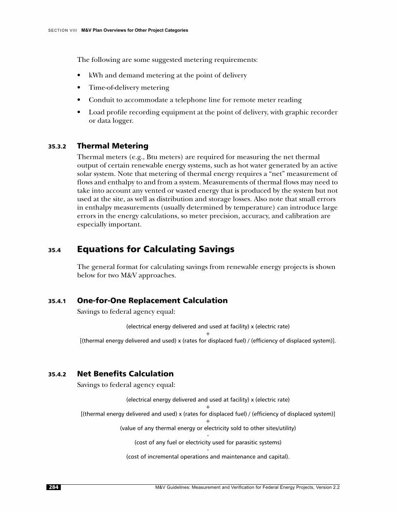
SECTION VII I M&V Plan Overviews for Other Project Categories
The following are some suggested metering requirements:
• kWh and demand metering at the point of delivery
• Time-of-delivery metering
• Conduit to accommodate a telephone line for remote meter reading
• Load profile recording equipment at the point of delivery, with graphic recorder or data logger.
35.3.2 Thermal MeteringThermal meters (e.g., Btu meters) are required for measuring the net thermaloutput of certain renewable energy systems, such as hot water generated by an active solar system. Note that metering of thermal energy requires a “net” measurement of flows and enthalpy to and from a system. Measurements of thermal flows may need to take into account any vented or wasted energy that is produced by the system but not used at the site, as well as distribution and storage losses. Also note that small errors in enthalpy measurements (usually determined by temperature) can introduce large errors in the energy calculations, so meter precision, accuracy, and calibration are especially important.
35.4 Equations for Calculating Savings
The general format for calculating savings from renewable energy projects is shown below for two M&V approaches.
35.4.1 One-for-One Replacement CalculationSavings to federal agency equal:
(electrical energy delivered and used at facility) x (electric rate)+
[(thermal energy delivered and used) x (rates for displaced fuel) / (efficiency of displaced system)].
35.4.2 Net Benefits CalculationSavings to federal agency equal:
(electrical energy delivered and used at facility) x (electric rate)+
[(thermal energy delivered and used) x (rates for displaced fuel) / (efficiency of displaced system)]+
(value of any thermal energy or electricity sold to other sites/utility)-
(cost of any fuel or electricity used for parasitic systems)-
(cost of incremental operations and maintenance and capital).
M&V Guidelines: Measurement and Verification for Federal Energy Projects, Version 2.2284
CHAPTER 35 Renewable Energy Projects
35.5 Notes on Renewable Energy Project M&V
35.5.1 Active Solar Thermal SystemsActive solar thermal systems include systems for producing industrial process heat, domestic hot water, and space heating and cooling. Useful monitoring includes (a) site inspections and brief temperature and system monitoring for diagnostics, (b) spot, short-term, or long-term monitoring of system key parameters such astemperatures, energy flows, and control status, and (c) utility billing analyses.
35.5.2 Passive Solar SystemsPassive solar systems usually involve the performance of a whole building witharchitectural features such as overhang design and use of thermal mass. As such, this technology is different from other renewable energy measures in that mechanical devices with identifiable energy inputs and outputs are not involved. Thus, passive solar M&V typically involves the analysis of a whole building and it is best to use utility billing analyses and calibrated simulation techniques—Options C and D.
35.5.3 Wind, PV, and Other Renewable Generation ProjectsWith these types of systems the performance characteristics of the components are usually well defined, such as the conversion efficiency of the PV modules or the Btu content of landfill gas. In addition, the electrical or thermal flows can usually beeasily measured. The complexity of these projects is in projecting long-termperformance due to variation in the resources (e.g., solar insolation, wind resource, or reserve of methane gas in a landfill) and accounting for any variations between when the resource is available and when it is needed—i.e., the interaction of storage systems and their inefficiencies.
35.6 Site-Specific Measurement and Verification Plan
M&V plans for renewable energy projects will need to be custom developed by the ESCO and the federal agency since each project is usually unique, and there are no guideline M&V methods (as there are for water and energy measures). The site-specific measurement and verification approach may be pre-specified in the ESPC contract between the federal agency and ESCO and/or agreed to after the awardof the project. In either case, prior to the federal agency's approval of projectconstruction, the ESCO will need to submit a final M&V plan that addresses thefollowing elements:
M&V Guidelines: Measurement and Verification for Federal Energy Projects, Version 2.2 285

SECTION VII I M&V Plan Overviews for Other Project Categories
• Describe the facility and the project; include information on how the project saves energy and/or provides non-energy benefits and what key variables effect the realization of savings. An accounting-type spreadsheet should be prepared which shows estimated baseline costs and projected performance period costsfor categories such as: electricity and fuel purchases (rates, total costs, andconsumption), labor, materials, and equipment replacement. Each of thesevalues will need to be verified (baseline) or determined during the pre- and post-installation M&V processes. To determine the savings from renewables projects (particularly demand savings), it is usually necessary to prepare time-of-useanalyses for typical days or week, if not for the whole year.
• Indicate how the federal agency's budget will be directly reduced by theimplementation of the project. All payments to ESCOs must come fromdemonstrable savings to the agency's budget.
• Define the minimum performance standards (e.g., minimum hot watertemperatures or voltage over- and under -frequency standards) that are currently in place and those required once the measure is in place. Determine how benefits (or losses) associated with improvements (or reductions) in performance standards will be allocated between parties. Indicate how compliance with performance standards will be verified during the term of the agreement.
• Indicate who will conduct the M&V activities and prepare analyses and documentation.
• Define the details of how calculations will be made and the assumptions that will be made about significant variables or unknowns. For instance: utility rate schedules (including stand-by rates) with and without the new renewables measures and sources for solar or wind resource data. Describe any stipulations that will be made and the source of data for the stipulations. Describe any tracking software that may be used. Show how calculations of savings will be used to determine payments to the ESCO.
• Specify what metering and data logging equipment will be used, who will provide the equipment, its accuracy and calibration procedures, and how data from the metering will be validated and reported, including formats. Electronic formatted data directly from a meter or data logger is usually required.
• Specify what additional management oversight logs will be maintained, the nature and frequency of entries, and the interpretation that is to be assigned to the results. Examples include logging equipment failures, equipment down time, and system outputs.
• Indicate how quality assurance will be maintained and repeatability confirmed. For instance, “The data being collected will be checked every month and provided to the federal agency.”
• Indicate which reports will be prepared, what they will contain, and when they will be provided.
M&V Guidelines: Measurement and Verification for Federal Energy Projects, Version 2.2286

AAppendix A: Definition of Terms
Note: If there is any discrepancy between the definitions in this document and those in the ESCO/federal agency contract, the definitions in the contract prevail.
Baseline Usage or Demand The calculated or measured energy usage (demand) by a piece of equipment or a site prior to the implementation of the project. Baselinephysical conditions such as equipment counts, nameplate data, and control strategies will typically be determined through surveys, inspections, and/or metering at the site.
Contract The executed document between a federal agency and the ESCO and any appendices, as amended from time to time, that outline provisions of the project.
Commissioning The process of documenting and verifying through adjusting/remedying the performance of building facility systems so that they operate inconformity with the design intent. An independent party rather than an ESCO may complete system/equipment commissioning. Current editions of the American Society of Heating, Refrigerating, and Air Conditioning Engineers' (ASHRAE) commissioning guideline GPC-1 can be the basis for commissioning activities.
Demand Reduction Estimates Energy demand reductions (e.g., in kW or Btu/hr) determined from metering and/or calculations performed in accordance with theprovisions of the federal agencies' approved measurement and verification plans, and documented in regular true-up reports.
Energy Savings Estimates Energy savings (e.g., in kWh or therms) determined from metering and/or calculations performed in accordance with the provisions of the federal agencies' approved measurement and verification plans, and documented in regular interval reports.
Energy Services Company (ESCO) An organization that designs, finances, procures, installs, and possibly maintains one or more ECMs or systems at a federal facility or facilities.
Measurements, Continuous Measurements repeated at regular intervals over the baseline period or contract term.
Measurements, Long-Term Measurements taken over a period of several years.
M&V Guidelines: Measurement and Verification for Federal Energy Projects, Version 2.2 287
APPENDIX A Definition of Terms
Measurements, Short-Term Measurements taken for several hours, weeks, or months.
Measurements, Spot Measurements taken one-time; snapshot measurements.
M&V Option One of four generic M&V approaches (A, B, C, and D) defined for ESPC projects. These options are defined in the International Performance Measurement and Verification Protocol (IPMVP) and in Chapter 2 of this document.
M&V Method A generic, non-project-specific M&V approach that applies one of the four M&V Options to a specific ECM technology category. Examples of ECM categories are lighting efficiency retrofits and constant-load motor retrofits.
M&V Technique An evaluation procedure for determining energy and cost savings. M&V techniques discussed in this document include engineering calculations, metering, utility billing analysis, and computer simulation.
Performance Factors Factors that influence energy use (e.g., outdoor air temperature, lighting levels, and timeclock settings).
Performance Period The time period spanning from approval of the project installation to the end of the contract.
Project Pre-Installation Report The initial report that provides a description and inventory of existing and proposed energy-efficiency equipment, estimates of energy savings, and a site-specific M&V plan (if not included in the contract). This report must be received and approved before the installation of energy-efficient equipment or O&M measures can occur.
Project Post-Installation Report The report that provides a description and inventory of baseline and installed energy-efficiency equipment, estimates of energy savings, and M&V results. After the installation of ECMs, the ESCO provides pre-specified documentation that verifies the installed equipment/systems, provides ECM energy saving estimates, and demonstrates proper commissioning has been completed.
Performance Period Energy Use or Demand The calculated energy usage (or demand) by a piece of equipment or a site after implementation of the project. The ESCO and the federal agency verify the post-installation energy use, the installation of the proper equipment components or systems, the correct operation of the components and systems, and their potential to generate the predicted savings.
Project The implementation of energy efficiency services at a federal facility or group of facilities.
Project-Specific M&V Plan Plan providing details on how a specific project's savings will be verified based on the general M&V approaches described in this document.
M&V Guidelines: Measurement and Verification for Federal Energy Projects, Version 2.2288

APPENDIX A Definition of Terms
Regular Interval Report Prespecified documentation provided by the ESCO at defined intervals (e.g., annually) during the performance period but after the submittal of the project post-installation report. This documentation verifies the continued operation of the ECMS, provides the associated energy savings estimates, demonstrates proper maintenance, and provides M&V results. The energy savings documented in the report serves as the basis for the ESCO's invoice after the regular interval report has been reviewed and approved by the federal agency.
Usage Group A collection of equipment (e.g., motors or rooms with light fixtures) with similar characteristics (e.g., operating schedule).
M&V Guidelines: Measurement and Verification for Federal Energy Projects, Version 2.2 289


B
Appendix B: Sample Metering Forms
M&V Guidelines: Measurement and Verification for Federal Energy Projects, Version 2.2 291
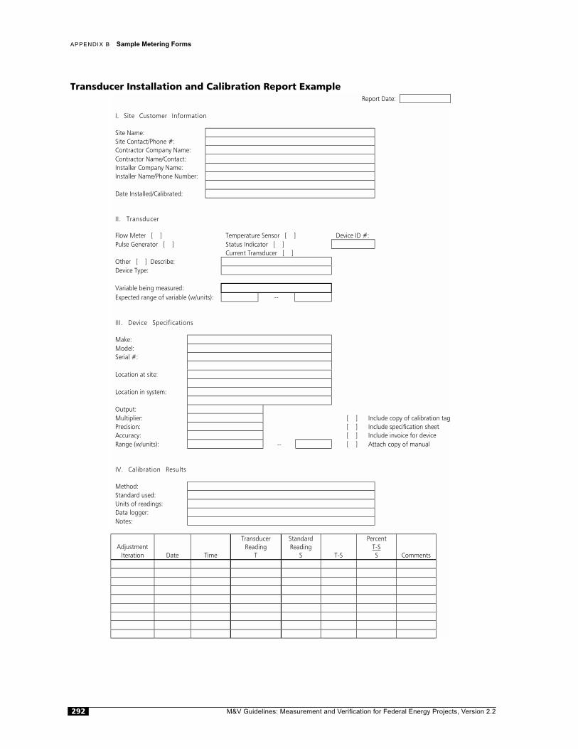
APPENDIX B
Sample Metering Forms
2
Tr
Report Date:I. Site Customer Information
Site Name:Site Contact/Phone #:Contractor Company Name:Contractor Name/Contact:Installer Company Name:Installer Name/Phone Number:
Date Installed/Calibrated:
II. Transducer
Flow Meter [ ] Temperature Sensor [ ] Device ID #:Pulse Generator [ ] Status Indicator [ ]
Current Transducer [ ]Other [ ] Describe:Device Type:
Variable being measured:Expected range of variable (w/units): --
III. Device Specifications
Make:Model:Serial #:
Location at site:
Location in system:
Output:Multiplier: [ ] Include copy of calibration tagPrecision: [ ] Include specification sheetAccuracy: [ ] Include invoice for deviceRange (w/units): -- [ ] Attach copy of manual
IV. Calibration Results
Method:Standard used:Units of readings:Data logger:Notes:
AdjustmentIteration Date Time
TransducerReading
T
StandardReading
S T-S
PercentT-SS Comments
ansducer Installation and Calibration Report Example
M&V Guidelines: Measurement and Verification for Federal Energy Projects, Version 2.292

APPENDIX B
Sample Metering Forms
Data Logger Report Example
Report Date:
I. Site/Installer Information
Site Name:Site Contact/Phone #:Contractor Company Name:Contractor Name/Contact:Installer Company Name:Installer Name/Phone Number:
Date Installed/Programmed:
II. Data Collection Information
Data Output Format:
Data Reporting Period:Storage Capacity of Data Logger:
Downloading Procedure:
Person/company responsible fordelivering data to federal agency:
III. Data Format
Channel Output UnitsExpected
RangeSampling
Rate
IV. Transducers
ChannelTransducer/Location
TransducerOutput
TransducerVendor/Model
TransducerInstall Date
TransducerCalibrated
M&V Guidelines: Measurement and Verification for Federal Energy Projects, Version 2.2 293


C
Appendix C: Sample Lighting and MotorSurvey Forms
M&V Guidelines: Measurement and Verification for Federal Energy Projects, Version 2.2 295
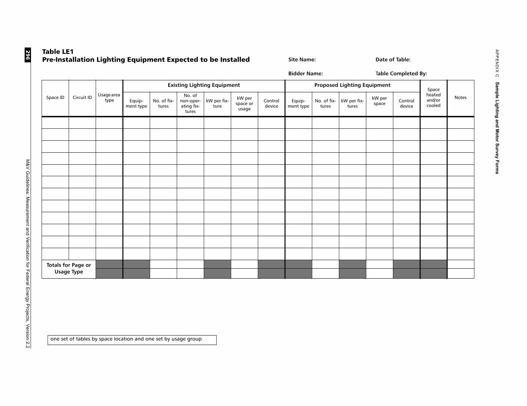
AP
PE
ND
IX C
Sam
ple L
igh
ting
and
Mo
tor S
urvey F
orm
s
M&
V G
uidelines: Measurem
ent and Verification for F
ederal Energy P
rojects, Version 2.2
29
6
TP
g Equipment
Space heated and/or cooled
Notes fix-s
kW per space Control
device
Date of Table:
T
able Completed By:
able LE1re-Installation Lighting Equipment Expected to be Installed
Space ID Circuit ID Usage area type
Existing Lighting Equipment Proposed Lightin
Equip-ment type
No. of fix-tures
No. of non-oper-ating fix-
tures
kW per fix-ture
kW per space or usage
Control device
Equip-ment type
No. of fix-tures
kW perture
Totals for Page or Usage Type
one set of tables by space location and one set by usage group
Site Name:
Bidder Name:
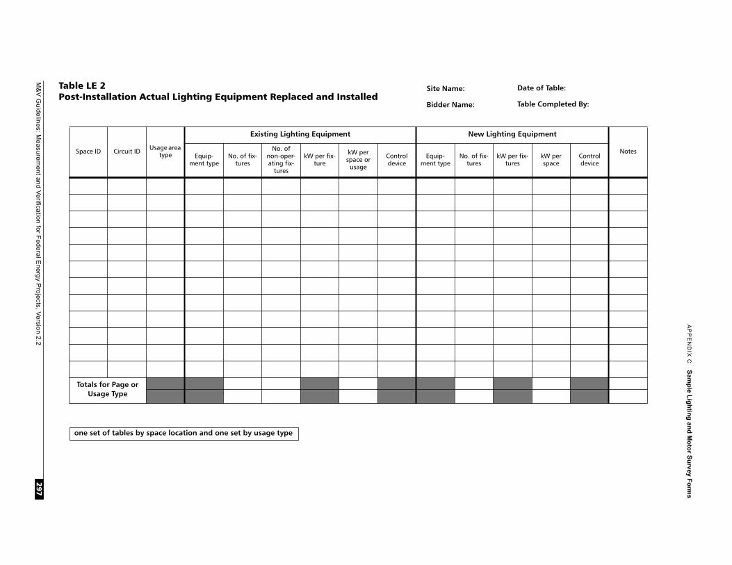
M&
V G
uidelines: Measurem
ent and Verification for F
ederal Energy P
rojects, Version 2.2
AP
PE
ND
IX C
Sam
ple L
igh
ting
and
Mo
tor S
urvey F
orm
s
297
TabPos
g Equipment
Notesper fix-ures
kW per space
Control device
Date of Table:
Table Completed By:
le LE 2t-Installation Actual Lighting Equipment Replaced and Installed
Space ID Circuit ID Usage area type
Existing Lighting Equipment New Lightin
Equip-ment type
No. of fix-tures
No. of non-oper-ating fix-
tures
kW per fix-ture
kW per space or usage
Control device
Equip-ment type
No. of fix-tures
kW t
Totals for Page or Usage Type
Site Name:
Bidder Name:
one set of tables by space location and one set by usage type
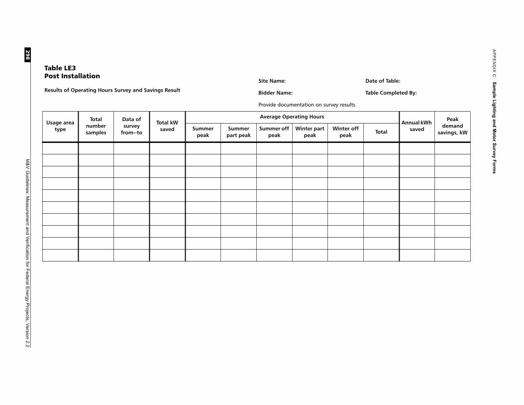
AP
PE
ND
IX C
Sam
ple L
igh
ting
and
Mo
tor S
urvey F
orm
s
M&
V G
uidelines: Measurem
ent and Verification for F
ederal Energy P
rojects, Version 2.2
29
8
Date of Table:
Table Completed By:
s
Annual kWh saved
Peak demand
savings, kWff
Total
Table LE3Post Installation
Results of Operating Hours Survey and Savings Result
Site Name:
Bidder Name:
Provide documentation on survey result
Usage area type
Total number samples
Data of survey
from--to
Total kW saved
Average Operating Hours
Summer peak
Summer part peak
Summer off peak
Winter part peak
Winter opeak

M&
V G
uidelines: Measurem
ent and Verification for F
ederal Energy P
rojects, Version 2.2
AP
PE
ND
IX C
Sam
ple L
igh
ting
and
Mo
tor S
urvey F
orm
s
299
TabAn
Res
Date of Table:
Table Completed By:
Usa Annual kWh saved
Peak demand
savings, kWTotal
le LE4nual Report
ults of Annual Operating Hours Survey and Savings Result
Site Name:
Bidder Name:
Provide documentation on survey results
ge area type
Total number samples
Data of survey
from--to
Total kW saved
Average Operating Hours
Summer peak
Summer part peak
Summer off peak
Winter part peak
Winter off peak
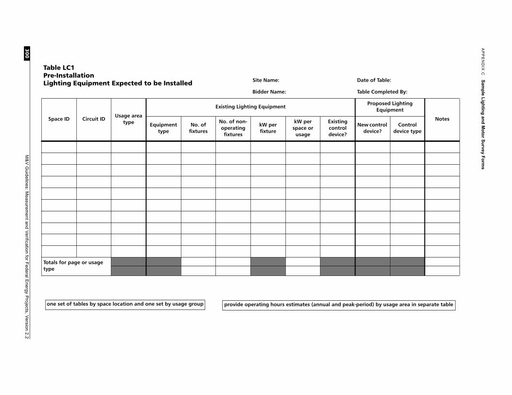
AP
PE
ND
IX C
Sam
ple L
igh
ting
and
Mo
tor S
urvey F
orm
s
M&
V G
uidelines: Measurem
ent and Verification for F
ederal Energy P
rojects, Version 2.2
30
0
Date of Table:
Table Completed By:
Proposed Lighting Equipment
Notes l
New control device?
Control device type
eak-period) by usage area in separate table
Table LC1Pre-InstallationLighting Equipment Expected to be Installed Site Name:
Bidder Name:
Space ID Circuit IDUsage area
type
Existing Lighting Equipment
Equipment type
No. of fixtures
No. of non-operating fixtures
kW per fixture
kW per space or
usage
Existingcontrodevice?
Totals for page or usage type
one set of tables by space location and one set by usage group provide operating hours estimates (annual and p
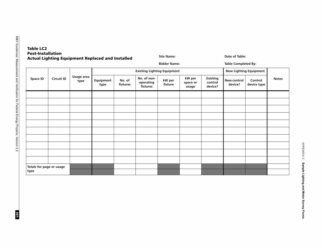
M&
V G
uidelines: Measurem
ent and Verification for F
ederal Energy P
rojects, Version 2.2
AP
PE
ND
IX C
Sam
ple L
igh
ting
and
Mo
tor S
urvey F
orm
s
301
TabPoAct
Date of Table:
Table Completed By:
Sp
New Lighting Equipment
NotesNew control device?
Control device type
Totatype
le LC2st-Installationual Lighting Equipment Replaced and Installed Site Name:
Bidder Name:
ace ID Circuit IDUsage area
type
Existing Lighting Equipment
Equipment type
No. of fixtures
No. of non-operating fixtures
kW per fixture
kW per space or
usage
Existing control device?
ls for page or usage

AP
PE
ND
IX C
Sam
ple L
igh
ting
and
Mo
tor S
urvey F
orm
s
M&
V G
uidelines: Measurem
ent and Verification for F
ederal Energy P
rojects, Version 2.2
30
2
Date of Table:
Table Completed By:
n on survey results
re-Installation
er part eak
Winter off peak
Total Annual
Table LC3Pre-InstallationResults of Operating Hours Survey Site Name:
Bidder Name:
Provide documentatio
Usage area type
Total number sampled
Dates of survey Total connected
kW
Average Operating Hours: P
From ToSummer
peakSummer part
peakSummer off
peakWint
p

M&
V G
uidelines: Measurem
ent and Verification for F
ederal Energy P
rojects, Version 2.2
AP
PE
ND
IX C
Sam
ple L
igh
ting
and
Mo
tor S
urvey F
orm
s
303
TabPoReRe
ble LC3
Us Annual kWh saved
Peak demand savings,
kWf
Total Annual
le LC4st-Installationsults of Operating Hours Survey and Savings sults
Site Name: Date of Table:
Bidder Name: Table Completed By:
Provide documentation on survey results
Savings based on difference in operating hours from Ta
age area type
Total number sampled
Dates of surveyTotal
connected kW
Average Operating Hours: Post-Installation
From ToSummer
peakSummer part peak
Summer off peak
Winter part peak
Winter ofpeak

AP
PE
ND
IX C
Sam
ple L
igh
ting
and
Mo
tor S
urvey F
orm
s
M&
V G
uidelines: Measurem
ent and Verification for F
ederal Energy P
rojects, Version 2.2
30
4
Table LC3
Annual kWh saved
Peak demand savings,
kWr off
akTotal Annual
Table LC5Annual ReportResults of Operating Hours Survey and Savings Results
Site Name: Date of Table:
Bidder Name: Table Completed By:
Provide documentation on survey results
Savings based on difference in operating hours from
Usage area type
Total number sampled
Dates of surveyTotal
connected kW
Average Operating Hours: Post-Installation
From ToSummer
peakSummer part peak
Summer off peak
Winter part peak
Wintepe

APPENDIX C
Sample Lighting and Motor Survey Forms
Table M1: Motor SurveyPre- and Post-Installation Data
Contractor Name:
Site Name:
Motor Location:
Motor Application:
complete during pre-installation complete during post-installation
Item Baseline High-Efficiency
Motor ID No.
Table Completed By
Date of Table
Nameplate Available (yes/no)
Manufacturer
Model No.
Serial No.
Service Factor
Enclosure Type
Full Load HP
Volts
Phase and Hz
Fill Load Amperes
Full Load Speed (RPM)
Synchronous Speed (RPM)
Nominal Efficiency
Load Served by Motor
Summer Weekday Operating Hours
Summer Weekend Operating Hours
Winter Weekday Operating Hours
Winter Weekend Operating Hours
Annual Operating Hours
Other
Complete for all motors
M&V Guidelines: Measurement and Verification for Federal Energy Projects, Version 2.2 305

APPENDIX C
Sample Lighting and Motor Survey Forms
Table M2: Spot Metered ValuesPre- and Post-Installation Data
Complete for all motors
Contractor Name:
Site Name:
Motor Location:
Motor Application:
pre-installation post-installation
Item Baseline High-Efficiency
Motor ID No.
Table Completed By
Date and Time of Readings
Instantaneous Volts
Instantaneous Amps
Instantaneous kW
Power Factor
Temp. of Working Fluid
Location of Temp. Sensor
Meter Model No.
Meter Serial No.
M&V Guidelines: Measurement and Verification for Federal Energy Projects, Version 2.2306
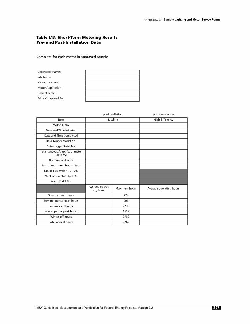
APPENDIX C
Sample Lighting and Motor Survey Forms
Table M3: Short-Term Metering ResultsPre- and Post-Installation Data
Complete for each motor in approved sample
Contractor Name:
Site Name:
Motor Location:
Motor Application:
Date of Table:
Table Completed By:
pre-installation post-installation
Item Baseline High-Efficiency
Motor ID No.
Date and Time Initiated
Date and Time Completed
Data-Logger Model No.
Data-Logger Serial No.
Instantaneous Amps (spot meter) Table M2
Normalizing Factor
No. of non-zero observations
No. of obs. within +/-10%
% of obs. within +/-10%
Meter Serial No.
Average operat-ing hours Maximum hours Average operating hours
Summer peak hours 774
Summer partial peak hours 903
Summer off hours 2739
Winter partial peak hours 1612
Winter off hours 2732
Total annual hours 8760
M&V Guidelines: Measurement and Verification for Federal Energy Projects, Version 2.2 307

APPENDIX C
Sample Lighting and Motor Survey Forms
Table M4: First Year Sample Selection and Results
To be completed for each unique application.
Contractor Name:
Site Name:
Date of Table:
Table Completed By:
Application Name:
Item Value
ID Nos. of motors serving application
Required sample size
ID Nos. of motors in sample
Average normalizing factor
Average summer peak operating hours
Average summer partial peak operating hours
Average summer off peak operating hours
Average winter partial peak operating hours
Average winter off peak operating hours
Average total annual operating hours
M&V Guidelines: Measurement and Verification for Federal Energy Projects, Version 2.2308
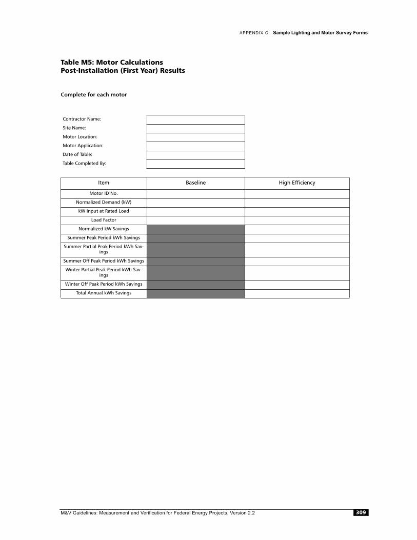
APPENDIX C
Sample Lighting and Motor Survey Forms
Table M5: Motor CalculationsPost-Installation (First Year) Results
Complete for each motor
Contractor Name:
Site Name:
Motor Location:
Motor Application:
Date of Table:
Table Completed By:
Item Baseline High Efficiency
Motor ID No.
Normalized Demand (kW)
kW Input at Rated Load
Load Factor
Normalized kW Savings
Summer Peak Period kWh Savings
Summer Partial Peak Period kWh Sav-ings
Summer Off Peak Period kWh Savings
Winter Partial Peak Period kWh Sav-ings
Winter Off Peak Period kWh Savings
Total Annual kWh Savings
M&V Guidelines: Measurement and Verification for Federal Energy Projects, Version 2.2 309

D
Appendix D: Sampling Guidelines
D.1 Introduction
This appendix introduces the statistical background, theory, and formulas used tocalculate sample sizes for monitoring purposes. It has been included for sampling designs that may be required for both lighting and non-lighting projects
This part provides guidelines for the procedures to follow to draw a sample forequipment monitoring. The guidelines are applicable to projects such as lightingretrofits and energy-efficient motor replacements, in which a large number of similar pieces of equipment are affected by the same type of ECM. The sampling guidelines are designed to help the ESCO and the federal agency determine the number ofsample points that should be monitored to provide a reliable estimate of parameters such as annual energy savings or hours of operation.
The purpose of monitoring a sample of equipment is twofold:
1. To measure operating patterns or other equipment characteristics used to estimate energy savings or other key parameters for the population from which the sample is drawn
2. To minimize monitoring costs while maintaining specified requirements for thereliability of the estimates
This information can be used to prepare project-specific M&V plans. This part includes 10 topics as follows:
• Part 2 states the general approach.
• Part 3 presents two sampling options.
• Part 4 explains the terminology used in the guidelines.
• Part 5 identifies the assumptions used in the sampling options.
• Part 6 presents the steps involved in calculating sample size.
• Part 7 discusses sample selection.
• Part 8 discusses verification of sample reliability and supplemental sampling.
M&V Guidelines: Measurement and Verification for Federal Energy Projects, Version 2.2 311
APPENDIX D
Sampling Guidelines
• Part 9 presents a lighting retrofit example using both sampling options.
• Part 10 summarizes the purpose of sampling.
D.2 General Approach
The sampling techniques in this section describe the procedures for selecting aproperly sized random sample of equipment for monitoring factors such asoperating hours. The measurements, taken from a sample of equipment, can then be used to estimate operating hours (which are used to calculate energy savings) for the entire population.
A successful sample will be sufficiently representative of the population to enable one to draw reliable inferences about the population as a whole. The reliability with which the sample-based estimate reflects the true population is based on specified statistical criteria, such as the confidence interval and precision level, used in the sample design.
The reliability of a sample-based estimate can be computed only after the metered data have been gathered. Before collecting the data, one cannot state the level of reliability that a given sample size will yield. However, one can compute the sample size that is expected to be sufficient to achieve a specified reliability level. This is done by using projections of certain values and criteria in the sample size calcula-tions. If the projections are too conservative, the estimate will exceed the reliability requirements. If these projections prove to be overly optimistic, then the reliability of the estimates will fall short of the requirements, requiring additional data collec-tion to achieve the specified reliability level. This method of using projections to cal-culate the necessary sample size is the one adopted for these guidelines.
The proposed sampling approaches consist of grouping the population of theequipment that is affected by the ECM's at the project site into “usage groups” from which samples are drawn. Usage groups are subsets of the entire population of affected equipment at the project site that have similar operating characteristics. Combining the affected equipment into homogeneous groups reduces the sample size required to obtain a reliable estimate. The proper designation of usage groups is critical for maintaining small sample sizes while still obtaining statistically valid results within specified confidence bounds.
In the first year of monitoring, the ESCO will use estimates of the average value and variability for key variables, e.g., operating hours of equipment for lighting projects in each usage group, in order to calculate the sample size required to achieve anestimate of the annual energy savings with the specified level of reliability. The ESCO will select sample points in each usage group randomly, as is consistent with statisti-cal practice.
After the required monitoring is performed on the sample of equipment, the ESCO will estimate the annual energy savings and compute the reliability of that estimate using metered data from the sample. If the reliability of the sample-based estimate falls short of the requirements of these guidelines, the ESCO will need to meter a
M&V Guidelines: Measurement and Verification for Federal Energy Projects, Version 2.2312
APPENDIX D
Sampling Guidelines
larger sample of equipment to achieve the necessary reliability requirements in the subsequent year.
In subsequent years of monitoring, the ESCO will use the results for averageoperating hours and their variances from the previous year's monitoring to calculate the necessary sample sizes. The formulas for calculating the variances based on the previous year's sample are presented in part D.6.
The perspective of this appendix is that a typical performance contractingarrangement, under the ESPC program, will be one in which the ESCO isresponsible for developing a detailed equipment inventory and sampling plan,conducting the metering, and analyzing savings. In contrast, the federal agency reviews and approves each step. Under some arrangements, the federal agency could develop the equipment inventory and sampling plan for the ESCO to follow. In that case, the federal agency would need to complete the tasks in this section that arecurrently assigned to the ESCO.
D.3 Sampling Options
Two sampling techniques discussed in these guidelines include:1
1. Building Level Sampling using stratified random sampling at the building level
2. Usage Group Sampling using simple random sampling at the usage group level, over multiple buildings.
D.3.1 Building Level SamplingThis approach includes guidelines for calculating sample size and allocating thesample across usage groups designed to achieve a specified level of precision for the savings estimate for a single building. The approach is based on an optimal allocation of sample points across the usage groups based on expected energy savings. This approach may be applied to a project with only one building, but has the advantage of reducing the overall number of required samples compared to usage groupsampling.
D.3.2 Usage Group SamplingA simple random sampling approach applies the precision criteria to each usage group within one or more buildings. This can lead to a higher-than-needed precision level for a single building. The advantages of this approach are (a) it is easy to implement, given a specified sample size table based on equipment population size; and (b) it permits sampling across buildings that are similar, are operated in the same manner, and have the same usage groups.
1. Schiller Associates developed these methodologies for various utility performance contracting pro-grams in collaboration with Dr. Andrew Goett of AAG and Associates and Dr. M. Sami Khawaja of Quan-tec.
M&V Guidelines: Measurement and Verification for Federal Energy Projects, Version 2.2 313
APPENDIX D
Sampling Guidelines
The key to the success of either of these approaches is that the ESCO properlydesignate usage groups.
D.4 Definitions
The guidelines presented here use certain terminology and notations that are defined as follows.
Last Point of Control (LPC). The last point of control (LPC) is defined as the portion of an electrical circuit that serves a set of equipment that is controlled on a single switch. As a result, all of the fixtures or pieces of equipment on that LPC are typically operated the same number of hours per year. For metering purposes, it is assumed that measurements taken of a single light fixture or piece of equipment on an LPC captures the operating hours for all of the equipment served on the same circuit. (Minor exceptions such as differences due to burnt-out bulbs and the like are ignored for these calculations.)
An example of an LPC would be a set of lighting fixtures in a room that operates on a single switch. If there were two separate switches controlling different groups offixtures in the room, each one would constitute an LPC for the metering purposes. In the formulas presented later, the total number of LPCs in the project or building is denoted by the population term N.
Usage Group. A usage group is a subset of the whole population of affectedequipment at the project site. Usage groups are designated for similar types ofequipment, similar areas, or with applications that have similar operatingcharacteristics. The designation of usage groups is based on equipment application and operating characteristics. This grouping technique subdivides a large group into smaller groups that are more homogeneous and thus reduces the variance of the projected operating hours in each group.2 By using building-level samplingtechniques, the number of LPCs that must be monitored to obtain an estimate with a given level of reliability is minimized. In the formulas presented later, usage groups are indexed by k. For example, the total number of LPCs in the usage group k is denoted by the term Nk.
Usage groups are not appropriately designated if they combine different functional groups with different operating patterns (e.g., offices and closets), lump smaller usage groups together (e.g., closets, storage, and utility rooms), or lump groups based on total annual hours but not operating function and pattern (e.g., offices and commons).
Project Site. A project site is any number of connected buildings. A project is the installation of measures at a project site
2.Care must be taken when designating usage groups, since too few groupings may result in higher vari-ances in operating hours and require a larger sample for each usage group in subsequent monitoring peri-ods. If there are too many groupings with too few points, the estimate of variance used for determining sample size in subsequent years will be poor and possibly lead to under-sampling.
M&V Guidelines: Measurement and Verification for Federal Energy Projects, Version 2.2314
APPENDIX D
Sampling Guidelines
Aggregation of Project Sites. For aggregation of project sites (i.e., multiple buildings) into a single project-specific M&V plan, all the project sites must have the same ESCO, measures, occupancy schedule, functional use, and energy consumptionpatterns.
Sample. The sample is the number of points (LPCs) that are monitored in each year. This sample must be drawn at random from the population of LPCs in each usage group, so that each LPC in a given usage group has the same likelihood of being selected to be monitored. The total sample size is denoted by n, and the sample in each usage group is nk. The percentage of circuits sampled in a given usage group is denoted by nk/Nk.
Sample Mean. The purpose of monitoring a sample of equipment or circuits is toestimate the mean or average value for one or more variables. For example, a typical objective of monitoring is to estimate the average hours of operation per year for the equipment that has been retrofitted with ECMs. The estimate of operating hours from the sample is used, in turn, to estimate the total energy savings.
Measures of Variability. The variance, standard deviation, standard error, andcoefficient of variation are measures of the variability of the values of the variable of interest (e.g., hours of operation) around the average. If the values are all clustered very close together, these measures are small. In the formulas presented latersection, the variance is denoted by S2(). The standard deviation is SD(), thestandard error is SE(), and the coefficient of variation is c.v.(). (c.v.() = SD()/mean())
Reliability Level. The reliability of a sample refers to the confidence with which one can state that the estimate produced by the sample falls within a specified range of the true value in the population. Any time an estimate of some variable such asaverage operating hours is based on measurements from a sample (rather than the entire population), the estimate typically will differ from the true value for thepopulation. This difference will vary from sample to sample, so that one cannot state with certainty the magnitude of any error in the estimate caused by using a sample. However, one can state the likelihood or probability that the estimate falls within some specified range of the true value for the population.
For example, one may be able to state that the probability is 95% that an estimate from a given sample falls within 100 hours of the true average number of operating hours per year. This means that if one drew 1,000 different independent samples, 95% of them would produce estimates within 100 hours of the population average. The probability (95%) is referred to as the confidence level. The specified range (100 hours) is the level of precision. This precision can be stated in absolute terms (±/-100 hours) or percentage terms (±/- 10%). By increasing the size of the sample used to produce the estimate, one can increase the reliability of the estimate (i.e., increase the confidence level, narrow the precision, or both).
Projected versus Estimated Total Savings and Its Variability. In the discussion below, the distinction is made between projected versus estimated values of the total savings and its variability. In order to calculate the sample size expected to achieve a
M&V Guidelines: Measurement and Verification for Federal Energy Projects, Version 2.2 315
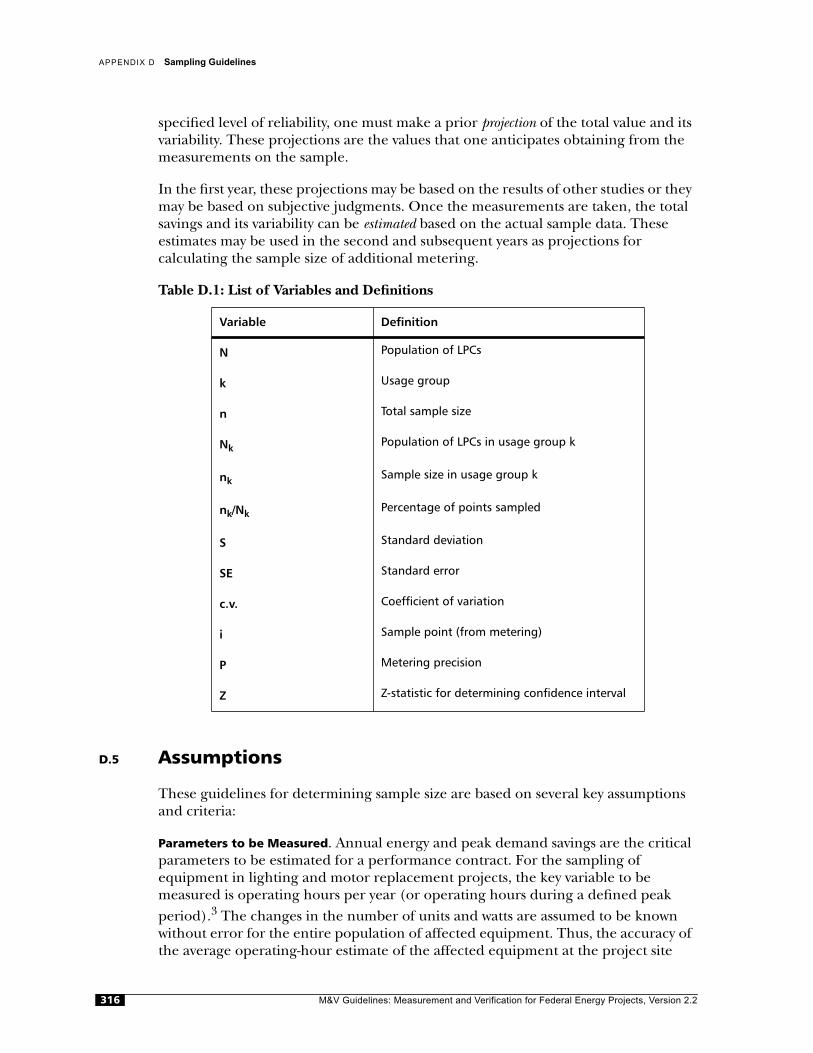
APPENDIX D
Sampling Guidelines
specified level of reliability, one must make a prior projection of the total value and its variability. These projections are the values that one anticipates obtaining from the measurements on the sample.
In the first year, these projections may be based on the results of other studies or they may be based on subjective judgments. Once the measurements are taken, the total savings and its variability can be estimated based on the actual sample data. Theseestimates may be used in the second and subsequent years as projections forcalculating the sample size of additional metering.
Table D.1: List of Variables and Definitions
D.5 Assumptions
These guidelines for determining sample size are based on several key assumptions and criteria:
Parameters to be Measured. Annual energy and peak demand savings are the critical parameters to be estimated for a performance contract. For the sampling ofequipment in lighting and motor replacement projects, the key variable to bemeasured is operating hours per year (or operating hours during a defined peak period).3 The changes in the number of units and watts are assumed to be known without error for the entire population of affected equipment. Thus, the accuracy of the average operating-hour estimate of the affected equipment at the project site
Variable Definition
N Population of LPCs
k Usage group
n Total sample size
Nk Population of LPCs in usage group k
nk Sample size in usage group k
nk/Nk Percentage of points sampled
S Standard deviation
SE Standard error
c.v. Coefficient of variation
i Sample point (from metering)
P Metering precision
Z Z-statistic for determining confidence interval
M&V Guidelines: Measurement and Verification for Federal Energy Projects, Version 2.2316
APPENDIX D
Sampling Guidelines
based on the sample is directly related to the accuracy level for the estimate of energy savings.
Sample Design Variable. For building level sampling, the variable that will be used to determine the required sample size is the annual electricity savings for the entire building or building in which the lighting or meter efficiency measures are installed. As a first-order approximation, the annual savings are equal to:
where:
• Savings = the annual energy savings for the build ing4
• ∆wattsk = the total change in wattage in usage group k
• = the average hours of operation per year of the equipment in usage group k.
Changes in Wattage. As part of the installation of ECMs, the ESCO records the change in wattage due to the replacement. As a result, the total change in wattage is known with certainty for all of the affected equipment in each usage group in the building.
Projection of Operating Hours. The ESCO makes a projection of the average operat-ing hours of the affected equipment in each usage group. Before the first year of monitoring, this may be a subjective judgment based on (a) the building operator's knowledge of how the affected equipment is typically used in each area; (b) a prior study of similar areas; or (c) a federal-agency-approved, pre-installation metering of a small sample in each usage group. After the first year, the metered results frommonitoring in the previous year will be used to determine the present-year sample size.
Reliability Level. The sample size needs to be sufficiently large to estimate the average annual operating hours within acceptable reliability requirements. What constitutes acceptable reliability is subject to discussion and negotiation. For example, utility DSM programs often use 90% confidence at 10% precision (90/10) or 80% confi-dence at 20% precision (80/20). (Both criteria are applied at the usage group level.) Which criteria are used depends on how reliable and accurate the utility company would like the savings estimates. What agencies and ESCOs need to realize is that increasing the reliability and accuracy of the savings estimates significantly increases
3. The formulas presented for calculating the necessary sample size are based on the assumption that the objective of the measurements is to estimate annual energy savings. If the objective is to estimate average kW reduction during the peak period, then the formulas would need to be modified by substituting a kWh variable with a kW variable.4. For purposes of calculating sample size, secondary effects, such as reduced internal loads caused by more efficient equipment, are ignored.
Savings ∆wattskk∑ OpHoursk×=
OpHoursk
M&V Guidelines: Measurement and Verification for Federal Energy Projects, Version 2.2 317
APPENDIX D
Sampling Guidelines
the effort required. Improving the precision from 20% to 10% will increase sample size (and M&V cost!) fourfold. Selecting the appropriate sampling criteria requires balancing accuracy requirements with M&V costs. Building-level sampling attempts to maximize accuracy while minimizing total sample size and M&V cost.
Oversampling. The initial sample size should be increased to compensate forpotential reductions in the final usable sample due to equipment failure or loss.Suggested guidelines are that the sample size be increased by 10% above the required amount.
D.6 Steps in Calculating Sample Size
The ESCO will calculate the number of pieces of equipment to be meteredaccording the following procedure:
1. Compiling ECM Information. As part of the installation of ECMs, the ESCO will compile the following information for the equipment affected by the measures:
– Number of LPCs. The ESCO will identify and document the LPCs that are affected by the installation of ECMs. This would be in the form of anequipment inventory survey in which each line in the survey represents an LPC that includes descriptions of affected and proposed ECM nameplate data and quantity as well as location information.
– Total Change in Wattage. Using the equipment inventory survey, the ESCO should tabulate the total change in wattage of the affected equipment by usage group.
– Projected Hours of Operation. The ESCO will project the average hours ofoperation of the equipment. This projection, which is distinguished from the estimate based on the monitoring, will be used solely for calculating the size and distribution of the sample required for monitoring. In the first year, it should be based on the experience of the building operator, on theoperation of the affected equipment or even some preliminary monitoring. After the first year of monitoring, the ESCO should use the estimate obtained from metering in the prior year to compute the sample size. If the ESCO expects that the equipment will be used in a significantly different manner in the current year than it was in the previous year, the estimate may be adjusted to reflect this, but only after the federal agency's review and approval.
– Expected Savings. The ESCO will project the expected annual savings from the ECMs installed in the building. This projection will be consistent with the change in wattage and projected hours of operation.
2. Designating Usage Groups. The ESCO will assign each LPC to a usage group based on similarities in equipment and operating characteristics as follows:
– Area type (e.g., office, hallway, bathroom)
– Annual operating hours
M&V Guidelines: Measurement and Verification for Federal Energy Projects, Version 2.2318

APPENDIX D
Sampling Guidelines
– Timing of the operating hours
– Variability of operating hours
– Similar functional use.
For the federal agency's project, a usage group is defined by equipment in the same area type for which the annual operating hours cluster around a specific estimate. At the same time, ESCOs should avoid designating usage groups with populations that will yield less than 10 points.
Sources of information on operating characteristics, other than monitoring, used in defining usage groups include the following: (a) operating schedules thatprovide information on energy consumption or hours of operation and (b) type of application or location that provides information on how and whenequipment (e.g., fixtures or motors) is operated.
Examples of standard usage groups for fan motors with similar operatingcharacteristics are HVAC ventilation supply fans, return fans, and exhaust fans. Examples of standard usage groups for lighting projects are fixtures with similar operating characteristics in offices, laboratories, hallways, stairwells, common areas, perimeters, and storage areas.
In some instances, area type alone may be insufficient to designate usage groups. Usage groups may need to be further subdivided if an area type is inherentlyvariable because area occupants have very different characteristics. For example, some laboratories may have longer operating hours than others and should be subdivided, if information is available that predicts the operating hours (e.g., computer laboratory hours are 8 hours per day while agriculture laboratory hours are 4 hours per day).
Usage groups will typically be defined for the population on a building-by-building basis. However, under special circumstances, for some projects it may be reasonable to determine sample sizes across a number of buildings with similar usage areas. For example, if an ESCO is conducting lighting retrofits in barracks, then the usage groups of common sleeping areas, private sleeping areas,washrooms, etc., may be totaled for all the barracks. These values can be usedto determine total population size for each usage group (assuming the usage group level sampling option is used). In applying the Usage Group Sampling approach, the samples would be selected from all the barracks. This would result in fewer monitoring points than if each building were considered separately.
3. Establishing Coefficient of Variation. In the first year of monitoring, the projec-tion of the coefficient of variation is typically drawn from other studies that have metered the operation of buildings with similar operating characteristics.However, under this guideline, the ESCO must use a coefficient of variation in each group of 0.5 as a default value. This assumption requires proper designation of homogeneous usage groups (where, in a given usage group, each point'sprojected operating hours vary no more than two standard deviations from the
M&V Guidelines: Measurement and Verification for Federal Energy Projects, Version 2.2 319
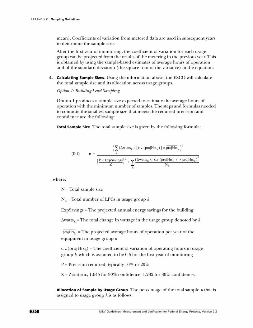
APPENDIX D
Sampling Guidelines
mean). Coefficients of variation from metered data are used in subsequent years to determine the sample size.
After the first year of monitoring, the coefficient of variation for each usage group can be projected from the results of the metering in the previous year. This is obtained by using the sample-based estimates of average hours of operation and of the standard deviation (the square root of the variance) in the equation.
4. Calculating Sample Sizes. Using the information above, the ESCO will calculate the total sample size and its allocation across usage groups.
Option 1: Building Level Sampling
Option 1 produces a sample size expected to estimate the average hours ofoperation with the minimum number of samples. The steps and formulas needed to compute the smallest sample size that meets the required precision andconfidence are the following:
Total Sample Size. The total sample size is given by the following formula:
where:
N = Total sample size
Nk = Total number of LPCs in usage group k
ExpSavings = The projected annual energy savings for the building
∆wattsk = The total change in wattage in the usage group denoted by k
= The projected average hours of operation per year of theequipment in usage group k
c.v.(projHrsk) = The coefficient of variation of operating hours in usage group k, which is assumed to be 0.5 for the first year of monitoring
P = Precision required, typically 10% or 20%
Z = Z-statistic, 1.645 for 90% confidence, 1.282 for 80% confidence.
Allocation of Sample by Usage Group. The percentage of the total sample n that is assigned to usage group k is as follows:
(D.1) n
∆wattsk c.v. projHrsk ) ]([× projHrs× k(k∑
2
P ExpSavings×Z--------------------------------------
2 ∆wattsk c.v. projHrsk([× ) ] projHrsk )×(
2
Nk-------------------------------------------------------------------------------------------------------
k∑+
--------------------------------------------------------------------------------------------------------------------------------------------------------------------=
projHrsk
M&V Guidelines: Measurement and Verification for Federal Energy Projects, Version 2.2320

APPENDIX D Sampling Guidelines
where:
nk = The sample size in usage group k; other terms are as defined above.
In the first year, the steps for computing the sample size and allocation are:
• Using (D.1), calculate the total sample size n based on the information on the change in wattage, projected hours of operation, and coefficient of varia-tion by usage group.
• Calculate the percentage of n to be allocated to each usage group (nk) based on the formula in equation (D.2), rounding the result up to the nearest whole number.
It is not possible to determine the reduction in sample size that building-level sampling provides compared to usage-group sampling without specific project information, but it can be significant if one usage group contributes significantly to the total uncertainty.
Option 2:Usage Group Sampling
Option 2 produces a sample size expected to estimate the average hours ofoperation with the required accuracy and confidence for each usage group in the building (or buildings). The steps and necessary formulas for computing the smallest sample size necessary to achieve these levels of precision and statistical confidence are the following:
Sample Size per Usage Group. The total sample size per usage group is given by the following formula:
where:
Z = Z-statistic, 1.645 for 90% confidence, 1.282 for 80% confidence
P = Precision required, typically 10% or 20%.
(D.2) nk∆wattsk c.v. projHrsk ) ] projHrsk×([×
∆wattsk c.v. projHrsk )([ ] projHrsk××k∑----------------------------------------------------------------------------------------------------- n×=
(D.3) nkZ2
c.v.[× projHrs) ]2
(
P2------------------------------------------------------=
M&V Guidelines: Measurement and Verification for Federal Energy Projects, Version 2.2 321
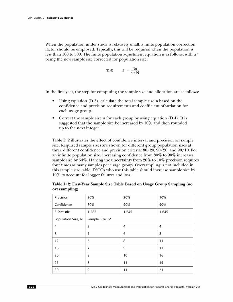
APPENDIX D Sampling Guidelines
When the population under study is relatively small, a finite population correction factor should be employed. Typically, this will be required when the population is less than 100 to 500. The finite population adjustment equation is as follows, with n* being the new sample size corrected for population size:
In the first year, the step for computing the sample size and allocation are as follows:
• Using equation (D.3), calculate the total sample size n based on theconfidence and precision requirements and coefficient of variation foreach usage group.
• Correct the sample size n for each group by using equation (D.4). It issuggested that the sample size be increased by 10% and then roundedup to the next integer.
Table D.2 illustrates the effect of confidence interval and precision on sample size. Required sample sizes are shown for different group population sizes at three different confidence and precision criteria: 80/20, 90/20, and 90/10. For an infinite population size, increasing confidence from 80% to 90% increases sample size by 54%. Halving the uncertainty from 20% to 10% precision requires four times as many samples per usage group. Oversampling is not included in this sample size table. ESCOs who use this table should increase sample size by 10% to account for logger failures and loss.
Table D.2: First-Year Sample Size Table Based on Usage Group Sampling (no oversampling)
Precision 20% 20% 10%
Confidence 80% 90% 90%
Z-Statistic 1.282 1.645 1.645
Population Size, N Sample Size, n*
4 3 4 4
8 5 6 8
12 6 8 11
16 7 9 13
20 8 10 16
25 8 11 19
30 9 11 21
(D.4) n* Nnn N+--------------=
M&V Guidelines: Measurement and Verification for Federal Energy Projects, Version 2.2322

APPENDIX D Sampling Guidelines
Selecting the appropriate sampling criteria depends on the acceptableuncertainty and the M&V budget. Much of the M&V cost is allocated to installing and removing loggers, so increasing sample size to improve reliability directly increases the M&V cost. Finding the most cost-effective sampling criteria is beyond the scope of this discussion, but the general idea is to avoid paying more for M&V than the value of the information returned.
D.7 Sample Selection and Equipment Metering
Given the values of nk, the samples in each usage group should be drawn at random,
so that each LPC has an equal probability of being selected.5 To allow for possible
35 9 12 24
40 9 12 26
45 9 13 28
50 10 13 29
60 10 14 32
70 10 14 35
80 10 15 37
90 10 15 39
100 10 15 41
125 11 15 45
150 11 16 47
175 11 16 49
200 11 16 51
300 11 17 56
400 11 17 59
500 11 17 60
infinite 11 17 68
Precision 20% 20% 10%
Confidence 80% 90% 90%
Z-Statistic 1.282 1.645 1.645
Population Size, N Sample Size, n*
5. Random selection of monitoring points is critical to avoid bias in the sample. Spreadsheet or other computer soft-ware should be used to generate a list of random numbers that may be used to place loggers on a given LPC.
M&V Guidelines: Measurement and Verification for Federal Energy Projects, Version 2.2 323
APPENDIX D Sampling Guidelines
attrition due to metering equipment failures and the like, the ESCO should monitor at least 10% more cases in each usage group than are required to meet the reliability requirement (i.e., the number of LPCs upon which meters are installed should be at least 110% of nk).
The metering period should be selected so that it is representative of equipment usage during the year. The metering should not be performed during periods with major holidays or when a significant portion of the building occupants are onvacation.
If there is reason to believe that there are significant seasonal variations in theaverage hours of operation of the equipment, the ESCO should conduct monitoring during different seasons. The ESCO should select the periods in each season that are representative of equipment usage. The average annual operating hours will beestimated by taking an average of the seasonal values, weighted by the number of months in each season.
D.8 Verification of Sample Reliability and Supplemental Sampling
After metering has been completed, the data will be used to calculate annualizedvalues for operating hours or another variable for which measurements have been taken. For example, if the equipment was metered for 21 days, then the estimate of annual operating hours would be the 21-typical-day total times 365/21 (365 days/year, 21 days monitored). The ESCO needs to ensure that the 21-day monitoring period does not include holidays that might bias the results.
Annualized values of operating hours will be used to estimate the total annual energy savings for the building and the standard error. These will be used to determine whether the reliability of the sample-based estimate meets the accuracy requirement. If the reliability of the estimate fails to meet the required level of confidence orprecision, the ESCO will be required to meter a larger sample of equipment to increase reliability in the following year. The size of this sample will be determined by substituting the metered estimates for the projected values and computing the necessary n and nk. The difference between the new values of n and nk and the old values is the supplemental sample size. A description of the procedure to use ispresented in the next section.
D.8.1 Building-Level VerificationEstimate the total savings and the standard error of the total according to thefollowing formulas:
M&V Guidelines: Measurement and Verification for Federal Energy Projects, Version 2.2324
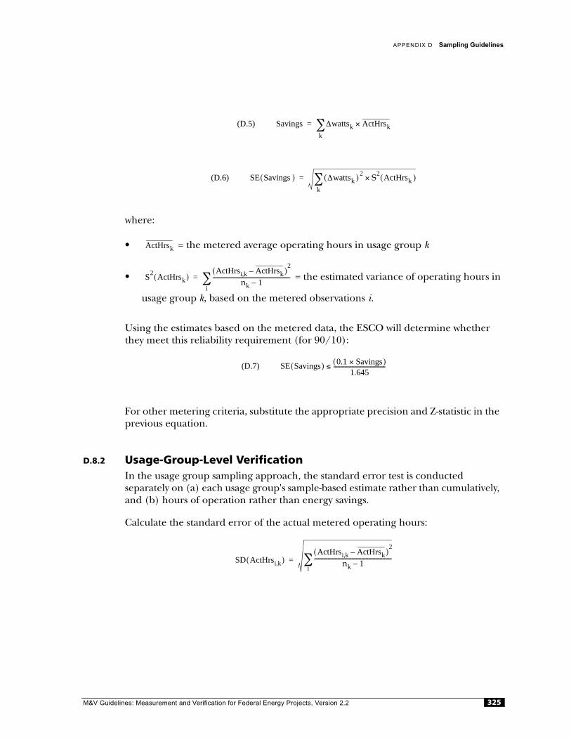
APPENDIX D Sampling Guidelines
where:
• = the metered average operating hours in usage group k
• = the estimated variance of operating hours in
usage group k, based on the metered observations i.
Using the estimates based on the metered data, the ESCO will determine whether they meet this reliability requirement (for 90/10):
For other metering criteria, substitute the appropriate precision and Z-statistic in the previous equation.
D.8.2 Usage-Group-Level VerificationIn the usage group sampling approach, the standard error test is conductedseparately on (a) each usage group's sample-based estimate rather than cumulatively, and (b) hours of operation rather than energy savings.
Calculate the standard error of the actual metered operating hours:
(D.5) Savings ∆wattsk ActHrsk×k∑=
(D.6) SE Savings( ) ∆wattsk )(2
k∑ S2
× ActHrsk )(=
ActHrsk
S2
ActHrsk( )ActHrsi,k ActHrsk–( )
2
nk 1–-------------------------------------------------------
i∑=
(D.7) SE Savings( ) 0.1 Savings×( )1.645
-------------------------------------≤
SD ActHrsi,k( )ActHrsi,k ActHrsk–( )
2
nk 1–-------------------------------------------------------
i∑=
M&V Guidelines: Measurement and Verification for Federal Energy Projects, Version 2.2 325
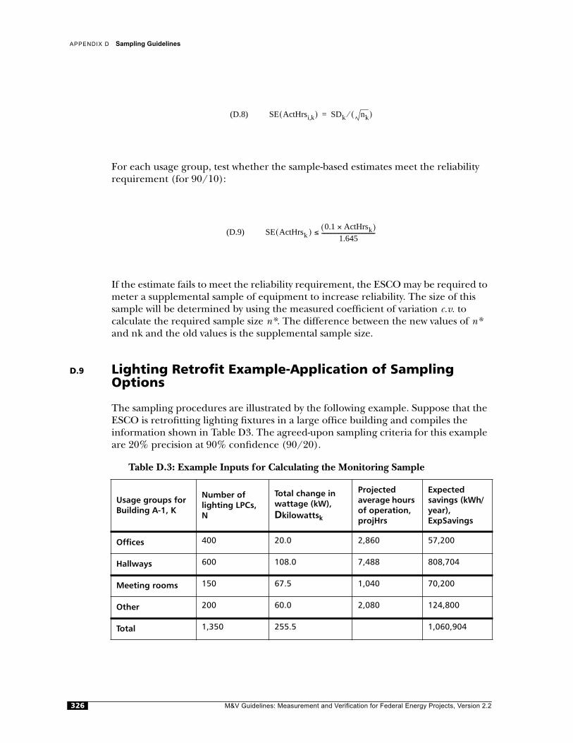
APPENDIX D Sampling Guidelines
For each usage group, test whether the sample-based estimates meet the reliability requirement (for 90/10):
If the estimate fails to meet the reliability requirement, the ESCO may be required to meter a supplemental sample of equipment to increase reliability. The size of this sample will be determined by using the measured coefficient of variation c.v. tocalculate the required sample size n*. The difference between the new values of n* and nk and the old values is the supplemental sample size.
D.9 Lighting Retrofit Example-Application of Sampling Options
The sampling procedures are illustrated by the following example. Suppose that the ESCO is retrofitting lighting fixtures in a large office building and compiles the information shown in Table D3. The agreed-upon sampling criteria for this example are 20% precision at 90% confidence (90/20).
Table D.3: Example Inputs for Calculating the Monitoring Sample
(D.8) SE ActHrsi,k( ) SDk nk( )⁄=
(D.9) SE ActHrsk )(0.1 ActHrsk×( )
1.645--------------------------------------≤
Usage groups for Building A-1, K
Number of lighting LPCs, N
Total change in wattage (kW), Dkilowattsk
Projected average hours of operation, projHrs
Expected savings (kWh/year), ExpSavings
Offices 400 20.0 2,860 57,200
Hallways 600 108.0 7,488 808,704
Meeting rooms 150 67.5 1,040 70,200
Other 200 60.0 2,080 124,800
Total 1,350 255.5 1,060,904
M&V Guidelines: Measurement and Verification for Federal Energy Projects, Version 2.2326

APPENDIX D Sampling Guidelines
D.9.1 Application of Building-Level SamplingThe sampling procedure varies with the following measurement cycle:
• First Measurement Period
Using the values shown in Table D.3 in Equation D.1 yields a total sample size of 64. According to Equation D.2, the percentage of sample in each usage group is calculated as shown in Table D4. After rounding, the total sample increases to 66. Table D.4 also presents the sample sizes adjusted by 10% for oversampling, which is suggested but not required.
• Subsequent Monitoring Periods
In the second and subsequent years, the same procedure will be used to calculate the sample size, with one exception: the values of and will be calculated from the data collected in the previous year's sample.
Table D.4: Example Sample Sizes by Usage Group
*A c.v.(y) = 0.5 is the default in the first measurement period; 10% additional sampling has been added to account for missing or malfunctioning loggers or improper usage group designations.
Note that the required total sample size without oversampling (66) is identical to what would be required using usage-group sampling (66 samples, but 16 or 17samples per group). The difference is that most of the building-level sampling has been concentrated in the hallway group because it represents the largest projectsavings and is thus the greatest contributor to the total uncertainty. This is a result of assuming a coefficient of variation for all groups of 0.5. In subsequent years, the total sample size and sample allocations will change when measured c.v.s are used.
Suppose that the ESCO obtains useful monitoring data for the required number of sample points and computes the standard errors of the operating hours and theestimated savings for each usage group presented in Table D.5. Using Equation D.6, one finds that the standard error of the total estimated savings is 408,815, which is above the value of 64,493 [%precision x expected savings/critical Z-statistic, or (0.1 x 1,060,904)/1.645] required to meet the reliability requirement.
Option 1: Building-Level Sampling (90/20)
Usage group, K nh nh (rounded) nh = 10% (rounded)*
Offices 3.4 4 5
Hallways 48.1 49 54
Meeting rooms 4.2 5 6
Other 7.4 8 9
Total 66 74
projHrsk c.v. projHrsk( )
M&V Guidelines: Measurement and Verification for Federal Energy Projects, Version 2.2 327
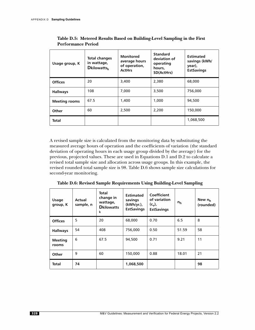
APPENDIX D Sampling Guidelines
Table D.5: Metered Results Based on Building-Level Sampling in the First Performance Period
A revised sample size is calculated from the monitoring data by substituting themeasured average hours of operation and the coefficients of variation (the standard deviation of operating hours in each usage group divided by the average) for the previous, projected values. These are used in Equations D.1 and D.2 to calculate a revised total sample size and allocation across usage groups. In this example, the revised rounded total sample size is 98. Table D.6 shows sample size calculations for second-year monitoring.
Table D.6: Revised Sample Requirements Using Building-Level Sampling
Usage group, KTotal changes in wattage, Dkilowattsk
Monitored average hours of operation, ActHrs
Standard deviation of operating hours, SD(ActHrs)
Estimated savings (kWh/year), EstSavings
Offices 20 3,400 2,380 68,000
Hallways 108 7,000 3,500 756,000
Meeting rooms 67.5 1,400 1,000 94,500
Other 60 2,500 2,200 150,000
Total 1,068,500
Usage group, K
Actual sample, n
Total change in wattage, Dkilowattsk
Estimated savings (kWh/yr.), EstSavings
Coefficient of variation (cv), EstSavings
nhNew nh (rounded)
Offices 5 20 68,000 0.70 6.5 8
Hallways 54 408 756,000 0.50 51.59 58
Meeting rooms
6 67.5 94,500 0.71 9.21 11
Other 9 60 150,000 0.88 18.01 21
Total 74 1,068,500 98
M&V Guidelines: Measurement and Verification for Federal Energy Projects, Version 2.2328
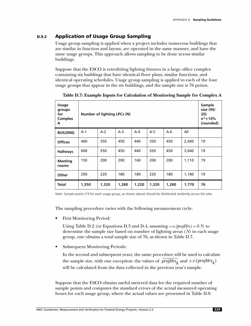
APPENDIX D Sampling Guidelines
D.9.2 Application of Usage Group SamplingUsage group sampling is applied when a project includes numerous buildings that are similar in function and layout, are operated in the same manner, and have the same usage groups. This approach allows sampling to be done across similarbuildings.
Suppose that the ESCO is retrofitting lighting fixtures in a large office complexcontaining six buildings that have identical floor plans, similar functions, andidentical operating schedules. Usage group sampling is applied to each of the four usage groups that appear in the six buildings, and the sample size is 76 points.
Table D.7: Example Inputs for Calculation of Monitoring Sample for Complex A
Note: Sample points (19 for each usage group, as shown above) should be distributed randomly across the sites.
The sampling procedure varies with the following measurement cycle:
• First Monitoring Period:
Using Table D.2 (or Equations D.3 and D.4, assuming c.v.(projHrs) = 0.5) todetermine the sample size based on number of lighting areas (N) in each usage group, one obtains a total sample size of 76, as shown in Table D.7.
• Subsequent Monitoring Periods:
In the second and subsequent years, the same procedure will be used to calculate the sample size, with one exception: the values of and will be calculated from the data collected in the previous year's sample.
Suppose that the ESCO obtains useful metered data for the required number of sample points and computes the standard errors of the actual measured operating hours for each usage group, where the actual values are presented in Table D.8.
Usage groups for Complex A
Number of lighting LPCs (N)
Sample size (90/20) n*+10% (rounded)
BUILDING A-1 A-2 A-3 A-4 A-5 A-6 All
Offices 400 350 450 440 350 450 2,440 19
Hallways 600 550 450 440 550 450 3,040 19
Meeting rooms
150 200 200 160 200 200 1,110 19
Other 200 220 180 180 220 180 1,180 19
Total 1,350 1,320 1,280 1,220 1,320 1,280 1,770 76
projHrskc.v. projHrsk( )
M&V Guidelines: Measurement and Verification for Federal Energy Projects, Version 2.2 329
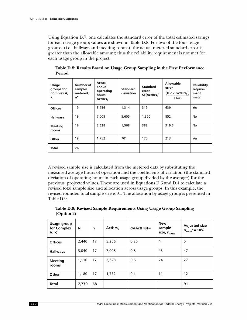
APPENDIX D Sampling Guidelines
Using Equation D.7, one calculates the standard error of the total estimated savings for each usage group; values are shown in Table D.8. For two of the four usage groups, (i.e., hallways and meeting rooms), the actual metered standard error is greater than the allowable amount; thus the reliability requirement is not met for each usage group in the project.
Table D.8: Results Based on Usage Group Sampling in the First Performance Period
A revised sample size is calculated from the metered data by substituting themeasured average hours of operation and the coefficients of variation (the standard deviation of operating hours in each usage group divided by the average) for the previous, projected values. These are used in Equations D.3 and D.4 to calculate a revised total sample size and allocation across usage groups. In this example, the revised rounded total sample size is 91. The allocation by usage group is presented in Table D.9.
Table D.9: Revised Sample Requirements Using Usage Group Sampling(Option 2)
Usage groups for Complex A, K
Number of samples metered, n*
Actual annual operating hours, ActHrsk
Standard deviation
Standard error, SE(ActHrsk)
Allowable error
Reliability require-ment met?
Offices 19 5,256 1,314 319 639 Yes
Hallways 19 7,008 5,605 1,360 852 No
Meeting rooms
19 2,628 1,568 382 319.5 No
Other 19 1,752 701 170 213 Yes
Total 76
Usage group for Complex A, K
N n ActHrsk cv(ActHrs)=New sample size, nnew
Adjusted size nnew*=10%
Offices 2,440 17 5,256 0.25 4 5
Hallways 3,040 17 7,008 0.8 43 47
Meeting rooms
1,110 17 2,628 0.6 24 27
Other 1,180 17 1,752 0.4 11 12
Total 7,770 68 91
0.2 ActHrsk×( )1.645
--------------------------------------
M&V Guidelines: Measurement and Verification for Federal Energy Projects, Version 2.2330

APPENDIX D Sampling Guidelines
D.10 Summary Note
Finally, keep in mind that the purpose of sampling is to monitor a representative sample of points rather than the entire population. The end result is to obtainreliable estimates within a specified precision and statistical confidence. Monitoring the specified number of points (that are calculated from the equations in thisappendix) does not necessarily mean the ESCO has complied with the requirements of the guidelines. The ESCO may have improperly designated usage groups, used incorrect sample design assumptions, or selected nonrandom points, all of which may lead to sample-based estimates that are biased and/or unreliable withinspecified levels. It is critical that the ESCO take care during the initial developmental stages to design a sample that truly reflects the project site.
The federal agency will examine the results of each year's worth of monitoring results of the measured average and variance(s) to establish the sample size in thesubsequent performance period.
M&V Guidelines: Measurement and Verification for Federal Energy Projects, Version 2.2 331


Prepared for the U. S. Department of Energy, FederalEnergy Management Program by Schiller Associates underthe direction of the National Renewable Energy Laboratoryand the Lawrence Berkeley National Laboratory
U. S. Department of EnergyOffice of Energy Efficiency and Renewable EnergyFederal Energy Management Program1000 Independence Ave., SWWashington, DC 20585
Lawrence Berkeley National laboratoryMS 90-3058Berkeley, California 94720510-486-4000
A U. S. Department of Energy national laboratory
National Renewable Energy Laboratory1617 Cole BoulevardGolden, Colorado 80401-3393303-275-3000
A U. S. Department of Energy national laboratory
Printed with a renewable-source ink on paper containing at least 50%wastepaper, including 20% post consumer waste.