Affirmative Action in Winner-Take-All Markets∗

Roland G. Fryer, Jr.† Glenn C. Loury‡

April 2005

Abstract

Whom to hire, promote, admit into elite universities, elect, or issue government contracts

to are all determined in a tournament-like (winner-take-all) structure. This paper constructs

a simple model of pair-wise tournament competition to investigate affirmative action in these

markets. We consider two forms of affirmative action: group-sighted, where employers are

allowed to use group identity in pursuit of their diversity goals; and group-blind, where they are

not. It is shown that the equilibrium group-sighted affirmative action scheme involves a constant

handicap given to agents in the disadvantaged group. Equilibrium group-blind affirmative action

creates a unique semi-separating equilibrium in which a large pool of contestants exerts zero

effort, and this pool is increasing in the aggresiveness of the affirmative action mandate.

∗We are grateful to Edward Glaeser, Jerry Green, and Bart Lipman for helpful comments and suggestions.†Harvard University Society of Fellows and NBER, 1875 Cambridge Street, Cambridge MA, 02138 (e-mail:

rfryer@fas.harvard.edu).‡Department of Economics, Boston University, 270 Bay State Road, Boston MA, 02215 (email: gloury@bu.edu).

1

1 Introduction

Winner-take-all markets are pervasive in our society. Whom to hire, promote, admit, elect, or

contract with are all determined in a tournament-like (winner-take-all) structure. In general, these

markets tend to emerge when there is quality variation, but little price flexibility. As a result, prizes

tend to be awarded on the basis of relative, not absolute, performance. Employment hiring and

promotion, admissions into elite universities, government contracts, or clerks to a supreme court

justice all have this feature in common.

Because of their structure, winner-take-all markets have the feature that small differences in

quality can be associated with large differences in rewards. This, coupled with the fact that many

of the controversial applications of affirmative action (mentioned above) involve winner-take-all

markets, makes it surprising that there has been no theoretical analysis of affirmative action in

these environments. Understanding the theoretical trade-offs involved when applying affirmative

action in winner-take-all markets is of great importance for public policy.

In this paper, we analyze affirmative action in winner-take-all markets. A short synopsis of our

approach is as follows. There are many positions and many more individuals seeking these positions.

Nature moves first and assigns a marginal cost of investment to each individual. Individuals observe

their exogenously-assigned cost of effort and choose the associated optimal level of effort to exert in

the contest. Nature, then, randomly assigns individuals to firms, where they are randomly matched

to compete in pair-wise contests. Absent any affirmative action target, the individual in each match

with the higher level of effort wins an exogenously determined prize.

We establish three main results. First, we solve explicitly for the equilibrium of a heterogeneous

tournament model. In the unique equilibrium, an individual’s behavioral strategy involves emitting

effort as a function of the distribution of individuals with cost above his. This leads naturally to

highly unequal outcomes between social groups endowed with different cost distributions and, hence,

a demand for affirmative action. We go on to analyze group-sighted and group-blind affirmative

action policies. The distinction between these two forms of redistribution turns on how group

information is used in the implementation of affirmative action policies. We show that the unique

equilibrium under group-sighted affirmative action involves a constant handicap for agents in the

disadvantaged group. Finally, when we impose the group-blind constraint, the nature of equilibrium

handicapping changes drastically. Under this formulation, a non-trivial measure of individuals pool

2

on a common low effort level and the prize is randomly distributed to members of the pool whenever

they are matched against one another.

These theoretical results have empirical relevance for the ongoing debate over affirmative action.

Recall, the unique equilibrium of our model under group sighted affirmative action involves a

constant handicap given to members of a disadvantaged group. This is similar, in particular, to the

practice of employing a lower minimum standardized test threshold for admission into elite colleges

and universities for minority applicants. Further, insisting on group-blind affirmative action — which

states such as California and Texas have done — is shown to undermine investment incentives for

all students in the long run.

This paper lies at the intersection of two literatures: tournament theory (Lazear and Rosen

1981, Green and Stokey 1983, Rosen 1986) and income redistribution (Mirrlees 1971, Akerlof 1978).

Our approach has little in common with the existing models in the tournament literature. These

models were developed to investigate the economic efficiency of tournament play and to analyze

tournaments as optimum labor contracts. In contrast, we focus on the implications of redistribution

in tournament-like environments.

The paper is related to the well studied problem of income redistribution. In the traditional op-

timal tax literature, individuals essentially pool their incomes and a central authority redistributes

the pool back to individuals in an incentive compatible manner. This approach is quite different

from our proposed framework. Affirmative action in winner-take-all contests imposes an additional

restriction on redistribution by constraining the employer to redistribute utility (i.e. the probability

of winning) using functionally irrelevant group identifiers in each match, but allowing employers

to reach their redistribution goals by aggregating outcomes across all of their matches. In other

words, when making a particular hiring decision, an employer must choose between a given slate

of candidates, but she evaluates those candidates with an eye toward achieving sufficient diversity

across all of her hiring decisions.

The exposition proceeds as follows: section 2 presents and solves our pair-wise tournament

model; section 3 analyzes group-sighted and group-blind affirmative action in our tournament

setup; and section 4 concludes.

3

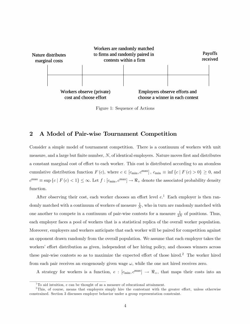
Nature distributesmarginal costs

Workers observe (private)cost and choose effort

Workers are randomly matched to firms and randomly paired in

contests within a firm

Employers observe efforts and choose a winner in each contest

Payoffsreceived

Nature distributesmarginal costs

Workers observe (private)cost and choose effort

Workers are randomly matched to firms and randomly paired in

contests within a firm

Employers observe efforts and choose a winner in each contest

Payoffsreceived

Figure 1: Sequence of Actions

2 A Model of Pair-wise Tournament Competition

Consider a simple model of tournament competition. There is a continuum of workers with unit

measure, and a large but finite number, N, of identical employers. Nature moves first and distributes

a constant marginal cost of effort to each worker. This cost is distributed according to an atomless

cumulative distribution function F (c), where c ∈ [cmin, cmax] , cmin ≡ inf {c | F (c) > 0} ≥ 0, and

cmax ≡ sup {c | F (c) < 1} ≤∞. Let f : [cmin, cmax]→ <+ denote the associated probability density

function.

After observing their cost, each worker chooses an effort level e.1 Each employer is then ran-

domly matched with a continuum of workers of measure 1N , who in turn are randomly matched with

one another to compete in a continuum of pair-wise contests for a measure 12N of positions. Thus,

each employer faces a pool of workers that is a statistical replica of the overall worker population.

Moreover, employers and workers anticipate that each worker will be paired for competition against

an opponent drawn randomly from the overall population. We assume that each employer takes the

workers’ effort distribution as given, independent of her hiring policy, and chooses winners across

these pair-wise contests so as to maximize the expected effort of those hired.2 The worker hired

from each pair receives an exogenously given wage ω, while the one not hired receives zero.

A strategy for workers is a function, e : [cmin, cmax] → <+, that maps their costs into an

1To aid intuition, e can be thought of as a measure of educational attainment.2This, of course, means that employers simply hire the contestant with the greater effort, unless otherwise

constrained. Section 3 discusses employer behavior under a group representation constraint.

4

effort decision. A strategy for an employer is an assignment function in each pair-wise match,

A : <2+ → [0, 1] , that maps the effort levels she observes in each contest to a probability of winning

for each worker in that contest. A worker presenting effort e wins against a worker presenting effortbe with a probability A (e, be) . Thus, the payoff to a worker if he wins the contest is ω − ce, while

the payoff is −ce if he loses.

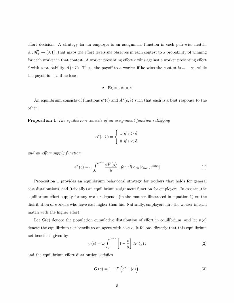
A. Equilibrium

An equilibrium consists of functions e∗(c) and A∗(e, be) such that each is a best response to theother.

Proposition 1 The equilibrium consists of an assignment function satisfying

A∗(e, be) =⎧⎨⎩ 1 if e > be0 if e < be

and an effort supply function

e∗ (c) = ω

Z cmax

c

dF (y)

y, for all c ∈ [cmin, cmax] (1)

Proposition 1 provides an equilibrium behavioral strategy for workers that holds for general

cost distributions, and (trivially) an equilibrium assignment function for employers. In essence, the

equilibrium effort supply for any worker depends (in the manner illustrated in equation 1) on the

distribution of workers who have cost higher than his. Naturally, employers hire the worker in each

match with the higher effort.

Let G(e) denote the population cumulative distribution of effort in equilibrium, and let v (c)

denote the equilibrium net benefit to an agent with cost c. It follows directly that this equilibrium

net benefit is given by

v (c) = ω

Z cmax

c

∙1− c

y

¸dF (y) ; (2)

and the equilibrium effort distribution satisfies

G (e) = 1− F³e∗−1(e)´. (3)

5

Notice that, taken together, equations (1) and (3) define a mapping from the exogenous cumulative

distribution of costs, F (c) , to the cumulative distribution of effort in equilibrium, G (e) , in the

natural way, which provides an explicit solution to the model.

To establish the proposition notice that, because workers choose effort to maximize their net

benefit, we have the first-order condition: ω ddeG(e)e=e∗(c) = c. A simple revealed preference ar-

gument establishes that e∗ (c) is non-increasing in c. Hence, equilibrium behavior implies that

G(e∗ (c)) ≡ [1− F (c)] . Putting these equations together, we have:

c = ωd

de[G(e)]e=e∗(c) = ω

d

dc[1− F (c)] · dc

de|{(e,c)|e=e∗(c)} .

Therefore, e∗ (c) satisfies the differential equation de∗

dc = −¡ωc

¢ ³dF (c)dc

´. Integrating this yields:

e∗ (c)− e∗ (cmax) = ω

Z cmax

c

dF (y)

y.

Finally, e∗ (cmax) = 0 since a worker with cost c = cmax loses with probability one. This establishes

the result.

B. Introducing Groups

Suppose now that employers can divide the population of workers into two identifiable groups.3

Let i ∈ {1, 2} index a worker’s group, and let πi > 0 denote the fraction of the worker population

belonging to group i, where π1 + π2 = 1. Hereafter, we use the subscript, i, to indicate group

identity. Thus, ei(c) denotes the effort exerted by a member of group i with cost c, Fi denotes

the cumulative distribution function of cost for group i workers, and Gi denotes the cumulative

distribution of effort (in equilibrium) among group i workers. We will assume throughout that the

cost distributions for the two groups have a common support.

Given our random matching assumptions, πi is also the probability that any worker, regardless

of his group, is paired to compete with a worker from group i. Since workers choose their effort

prior to being paired against an opponent, and because they are assigned randomly to firms and

then paired with each other at random for competition within firms, every worker faces the same

3These groups can be defined in terms of race, gender, social class, so on and so forth.

6

distribution of opponents (i.e., a statistical replica of the overall worker population.) Thus, despite

any asymmetry between groups that arises when F1(c) 6= F2(c), the workers paired to compete

with one another are playing a symmetric game. So, absent any group-based policy intervention,

the equilibrium behavior of firms and of workers (whatever their group) will be as described in

Proposition 1, with F (c) ≡ π1F1(c) + π2F2(c).

Now, with two distinct groups, three types of matches are possible: a group 2 worker can be

matched with a group 2 worker, which occurs with probability π22; a group 1 worker can be matched

with a group 1 worker, which occurs with probability π21; and a mixed match (between group 1

and group 2 workers) occurs with probability 2π1π2. We will assume that group 1 is “advantaged”

relative to group 2, in that the group 1 cost distribution monotonically first-order stochastically

dominates that of group 2.

Definition 1 Group 1 is said to be advantaged relative to group 2, if f1(c)f2(c)

is a strictly decreasing

function on (cmin, cmax) .

This definition implies F1(c) > F2(c) for all c ∈ (cmin, cmax). Let γ0 denote the probability

that a group 1 worker wins when matched with a group 2 worker, in the laissez-faire equilib-

rium described in Proposition 1. We refer to γ0 as the “natural win rate” of group 1 agents over

group 2 agents. Given Definition 1, it is intuitively obvious and straightforward to show that

γ0 ≡R cmaxcmin

dF1 (c) [1− F2 (c)] >12 .4

Because of the asymmetries in the cost distributions there will be a short-fall in the share of

group 2 agents hired by the employer, relative to their share of the worker population. Specifically,

the proportion of contests won by group 2 workers is

π22 + 2π2(1− π2)(1− γ0) < π2,

4To make this transparent, notice that:Z cmax

cmin

dF1 (c) [1− F2 (c)] =

Z cmax

cmin

dF1 (c) [1− F1 (c)] +

Z cmax

cmin

dF1 (c) [F1 (c)− F2 (c)] (4)

and Z cmax

cmin

dF1 (c) [1− F1 (c)] = −1

2

Z cmax

cmin

d

dc{[1− F1 (c)]

2} = 1

2. (5)

Further, under the assumption that group 2 is disadvantaged,R cmaxcmin

dF1 (c) [F1 (c)− F2 (c)] is necessarily a positive

number. Thus, we have the desired inequality.

7

in view of the fact that γ0 >12 . Thus, a demand for affirmative action could naturally arise here.

This is the subject of the next section.

3 Affirmative Action

Affirmative action involves equilibrium handicapping of workers in the disadvantaged group by

employers who take the distribution of worker effort as exogenous when setting the handicap.5 For

instance, a set of universities designing their admissions policies to ensure sufficient diversity, each

of which thinks its policies are unlikely to affect the effort distribution in the pool of college bound

seniors from which its applicants are drawn, is a case of affirmative action.

We will also employ the distinction between blind and sighted affirmative action. Blind versus

sighted refers to what markers employers are allowed to use in the pursuit of their affirmative

action policies. Group-sighted handicapping allows employers to use group identification directly in

achieving their redistributive target. Group-blind handicapping forbids the use of group information

in achieving diversity goals.

A. Group-Sighted Affirmative Action

Suppose a regulator wants to decrease the win rate of the advantaged group, and let γ ∈ [12 , γ0)

denote the target level of diversity.6 Notice that, as γ → γ0, the laissez-faire equilibrium described

in Proposition 1 obtains, while as γ → 12 , the employer is forced to achieve group parity.

It is straightforward to show that if an employer desires to maximize the expected effort of

the contestants, subject to the constraint that agents from the advantaged group only win at the

rate γ ∈£12 , γ0

¢when matched with an agent from the disadvantaged group, then the best way to

do so is to give group 2 workers a constant effort handicap, λ∗ (γ) . In particular, the employers’

optimization problem implies the maximization of a Lagrangian form as follows:

maxA

½Z ∞

0

Z ∞

0[A (e1, e2) e1 + (1−A (e1, e2)) e2 + λ (γ −A (e1, e2))] dG1(e1)dG2(e2)

¾(6)

5For concreteness, one can think about affirmative action in this context as coming about because all employersare required by some external authority to increase their hiring rate for workers in the disadvantaged category, thougheach employer acts independently of the others to achieve this goal.

6That is, γ denotes the target win rate of group 1 workers when matched against opponents from group 2. Noticethat, under sighted affirmative action, these are the only matches that a regulator would seek to influence.

8

Obviously, the solution must takes the form:

A (e1, e2) =

⎧⎨⎩ 1 if e∗1 (c) > e∗2 (c) + λ∗ (γ)

0 if e∗1 (c) < e∗2 (c) + λ∗ (γ), (7)

where λ∗(γ) is the Lagrangian multiplier on the redistribution constraint. (In effect, λ∗(γ) is the

“shadow price of diversity” when the redistribution target is γ.) Thus, the equilibrium handicap is

independent of the effort levels of the contestants, and varies positively with the aggressiveness of

the diversity goal.

It follows that, if e∗i (c) denotes the equilibrium effort supply of workers in group i ∈ {1, 2}, then

when an agent from group 1 is matched with an agent from group 2, the agent in group 1 wins the

contests if

e∗1 (c) > e∗2 (c) + λ∗ (γ) .

Notice that a group 1 worker who exerts low effort, e1 ∈ (0, λ∗), must lose if matched with any

group 2 worker.

We will now derive the equilibrium in this model under group-sighted affirmative action with

target γ ∈ [12 , γ0). Suppose there is an effort cost threshold, c∗ (γ) , such that group 1 agents

with cost c1 ≥ c∗ (γ) lose when matched with any group 2 agents, and group 1 agents with cost

c1 < c∗ (γ) , win when matched with any agent with higher cost.7 Then, by the affirmative action

constraint:

c∗ (γ) solvesZ c∗

cmin

dF1 (c) [1− F2 (c)] = γ. (8)

Notice, c∗ (γ) is increasing in γ, and c∗ (γ) tends toward cmax, as γ tends toward γ0; the natural

win rate of group1 agents over group 2’s.

To solve the model for any desired level of affirmative action, γ ∈£12 , γ0

¢, we must solve for the

equilibrium affirmative action handicap, λ, and the associated equilibrium effort levels. This is the

subject of our next result.

Proposition 2 Given γ ∈£12 , γ0

¢and c∗ (γ) defined in equation (8), the equilibrium group-sighted

7We shall show momentarily that in the presence of constant effort handicapping for category 2 agents theequilibrium effort supply functions imply this property.

9

affirmative action handicap is given by

λ∗ (γ) = ω

"π2

Z cmax

c∗(γ)

∙1

c∗ (γ)− 1

y

¸dF2 (y) + π1

Z cmax

c∗(γ)

dF1 (y)

y

#, (9)

the associated effort levels are given by

e∗1 (c) = e∗2 (c) + λ∗ (γ) = ω

"π1

Z cmax

c

dF1 (y)

y+ π2

"Z c∗(γ)

c

dF2 (y)

y+

Z cmax

c∗(γ)

dF2 (y)

c∗ (γ)

##,

for all c ∈ [cmin, c∗ (γ)) , and

e∗1 (c) = ωπ1

Z cmax

c

dF1 (y)

y; e∗2 (c) = ωπ2

Z cmax

c

dF2 (y)

y

for all c ∈ [c∗ (γ) , cmax] .

Proposition 2 provides a solution to the group-sighted affirmative action handicapping problem.

The result depends critically on three factors: (1) constant marginal cost of effort; (2) setting of

handicaps by many independent employers facing affirmative action regulation; and (3) random

matching. The solution implies a partition of agents into four classes: {group 1 or 2}×{high cost

(c ≥ c∗ (γ)) or low cost (c < c∗ (γ))}. For convenience of exposition, let Hi (resp. Li) denote the

set of high (resp. low) cost types of group i ∈ {1, 2} . The equilibrium behavior of the agents under

group-sighted affirmative action handicapping can be summarized in the following concise manner.

H 0is only compete at the margin against other H

0is in their same group, and lose to L

0is in either

group. Further, L0is compete at the margin against anyone with whom they are matched, prevailing

if and only if they encounter a contestant with higher cost. However, L02s receive the effort subsidy

λ∗ (γ) , such that e∗1 (c) = e∗2 (c) + λ∗ (γ) for all c ∈ [cmin, c∗ (γ)) . Figure 2 provides a graphical

illustration of Proposition 2.

10

0

A

B

λ

c*

MB

e c1*( ) e c2

*( ) + λ e e c e c= = +1 2* *( ) ( ) λ

( )MB F c1 1 1= ωπ '( ) ( )MB F c2 2 21= − +ω π λ'

0

A

B

λ

c*

MB

e c1*( ) e c2

*( ) + λ e e c e c= = +1 2* *( ) ( ) λ

( )MB F c1 1 1= ωπ '( ) ( )MB F c2 2 21= − +ω π λ'

Figure 2: Group-Sighted Affirmative Action Equilibrium

To establish the proposition, let e = e1 = e2 + λ denote effective effort supply of agents,

when group 2 workers receive the effort handicap λ. Given that, in equilibrium, ei ≥ 0 and

ei (cmax) = 0, i = 1, 2, there exist a set of high costs agents in both groups (i.e., those with c “close

to” cmax) who supply relatively low effort. For group 1 agents this implies e = e1 ≈ 0, and for group

2 agents this implies that e = e2+λ ≈ λ > 0. Thus, group 1 agents will face a non-convex decision

problem, in equilibrium, since at very low effort levels (e1 < λ) they compete only against other

high cost group 1 agents. At levels e1 > λ, they discontinuously encounter additional benefits from

marginal increases in effort, due to the presence of some high cost group 2 agents who are choosing

e2 ≈ 0, so e2 + λ ≈ λ. Figure 2 captures this intuition. Because group 1’s marginal benefit curve

jumps upward at λ, it must be the case that the optimal effort function e∗1 (c) is discontinuous. At

cost c = c∗ the area (in Figure 2) A ≡ [λ− e1 (c∗)] · c∗ is exactly equal (by construction) to the area

B ≡R e2(c∗)+λλ [MB2 (e)− c∗] de. Therefore, H 0

1s prefer e∗1(c) < λ, along the MB1 curve, whereas

L01s prefer to “jump” past λ to some e∗1(c) > e2 (c

∗) + λ. In other words, all H 01s choose to lose to

all group 2 agents, should they end-up paired with one, and compete at the margin only against

other H 01s; and all L

0is lose only if they are matched with a worker who has lower cost. When λ

has been set such that the constraint that workers in group 1 win against workers in group 2 with

probability γ ∈£12 , γ0

¢holds, then it is straightforward to verify that we must have c∗ = c∗ (γ)

11

defined in equation (8).

Using equation (1) and noting that H 0is only compete at the margin against other H

0is in the

same group, we deduce that the marginal benefit for group 1 and group 2 agents can be expressed

as:

MB1 (e) = c if and only if e = ωπ1

Z cmax

c

dF1 (y)

y≡ e∗1 (c)

MB2 (e) = c if and only if e = ωπ2

Z cmax

c

dF2 (y)

y≡ e∗2 (c)

Recall, however, H 01s always have the option of boosting their effort to compete with group 2

workers. This is a break-even proposition when c = c∗ and strictly pays if c < c∗. Hence, for all

c < c∗, the effort supply function looks much like that in Proposition 1. Both groups supply the

same effective effort, given their cost, and e∗ (c) solves the differential equation:

de∗

dc= −ω

c

dF

dc= −ω

c

£π1F

01 (c) + π2F

02 (c)

¤, (10)

as in Proposition 1, but with the boundary condition: e∗ (c∗) = e∗2 (c∗) + λ. Finally, λ must satisfy

c∗ [λ− e∗1 (c∗)] = v2 (c

∗)

where, using equation (2), v2 (c) = ωπ2R cmaxc

h1− c

y

idF2 (y) . By integrating equation (10), using

the relevant boundary conditions and definitions derived thus far, the conditions of the Proposition

can be easily verified by algebraic manipulation.

B. Group-Blind Affirmative Action

The employer’s problem is more complicated when she is not allowed to use group information

in the pursuit of her affirmative action goals. Employers observe two effort levels in each match,

e and be, but under the blindness assumption they do not know the group identity of the workers.Accordingly, to achieve their diversity objectives, employers need to estimate the likelihood that

each effort level was emitted from a worker in the disadvantaged group. Thus, we overlay a signalling

model on top of our pairwise competitive framework. This is a point worth further emphasis. Under

group-sighted affirmative action an employer is allowed to narrowly tailor her policies for agents in

12

disadvantaged groups in order to achieve her diversity goal — focusing exclusively on handicapping

in mixed contests. When constrained to be group-blind, however, she has to implement her policy

across all contests. This is especially inefficient when the disadvantaged group is a small share of

the population.

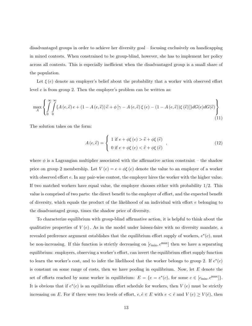
Let ξ (e) denote an employer’s belief about the probability that a worker with observed effort

level e is from group 2. Then the employer’s problem can be written as:

maxA

⎧⎨⎩∞Z0

∞Z0

{A (e, be) e+ (1−A (e, be)) be+ φ [γ −A (e, be) ξ (e)− (1−A (e, be))ξ (be)]}dG(e)dG(be)⎫⎬⎭(11)

The solution takes on the form:

A (e, be) =⎧⎨⎩ 1 if e+ φξ (e) > be+ φξ (be)0 if e+ φξ (e) < be+ φξ (be) , (12)

where φ is a Lagrangian multiplier associated with the affirmative action constraint — the shadow

price on group 2 membership. Let V (e) = e+ φξ (e) denote the value to an employer of a worker

with observed effort e. In any pair-wise contest, the employer hires the worker with the higher value.

If two matched workers have equal value, the employer chooses either with probability 1/2. This

value is comprised of two parts: the direct benefit to the employer of effort, and the expected benefit

of diversity, which equals the product of the likelihood of an individual with effort e belonging to

the disadvantaged group, times the shadow price of diversity.

To characterize equilibrium with group-blind affirmative action, it is helpful to think about the

qualitative properties of V (e) . As in the model under laissez-faire with no diversity mandate, a

revealed preference argument establishes that the equilibrium effort supply of workers, e∗(c), must

be non-increasing. If this function is strictly decreasing on [cmin, cmax] then we have a separating

equilibrium: employers, observing a worker’s effort, can invert the equilibrium effort supply function

to learn the worker’s cost, and to infer the likelihood that the worker belongs to group 2. If e∗(c)

is constant on some range of costs, then we have pooling in equilibrium. Now, let E denote the

set of efforts reached by some worker in equilibrium: E = {e = e∗(c), for some c ∈ [cmin, cmax]}.

It is obvious that if e∗(c) is an equilibrium effort schedule for workers, then V (e) must be strictly

increasing on E. For if there were two levels of effort, e, e ∈ E with e < e and V (e) ≥ V (e), then

13

any worker choosing e could gain by reducing his level of effort to e, which lowers his cost incurred

without lowering his chances of winning the contest. But, from this it follows that a separating

equilibrium cannot obtain here. For, if e∗(c) were strictly monotonic on (cmin, cmax), and if V (e)

were strictly increasing on E, then a worker would not be hired whenever matched against another

worker with lower cost8, in which case the affirmative action constraint could not be satisfied. We

conclude that there must be some pooling in equilibrium. That is, the equilibrium effort supply

function, e∗(c), must be constant over some non-empty interval(s) of costs. Moreover, a worker in

the pool would be hired (not hired) with probability one when paired with a worker whose effort

level is lower (higher) than that of the pool, and would be hired with probability 1/2 when paired

with another worker in the pool. The size of the pool will increase with the aggressiveness of the

diversity goal.

This situation is captured in Figures 3, which show a pooling equilibrium where all worker types

c in the closed interval [bc,bbc] select the common effort level, epool. Figure 3A depicts a worker’s

value to the employer as a function of his effort. Figure 3B shows the worker’s best response to the

employer strategy “hire that worker with the greater value,” as a function of the worker’s cost.

eee

)(eV e

cc c

A B

poole

e

poole

e

eee

)(eV e

cc c

A B

poole

e

poole

e

Figure 3: Group-Blind Affirmative Action Equilibrium

8Ties will occur with probability zero when e∗(c) is strictly monotonic, since we have assumed the cost distributionto be non-atomic.

14

In any equilibrium under group-blind affirmative action several conditions need to be satisfied,

all of which can be illustrated in Figures 3.9 First, the worker with marginal cost bc must beindifferent between leaving the pool by putting in effort be, which would imply that he wins forsure against all workers in the pool, and exerting the effort epool, which has him winning with

probability 12 when matched with anyone in the pool. Similarly, the worker with cost bbc must

be indifferent between staying with the pool, and reducing his effort to bbe. Also, firms must beindifferent between hiring from the pool, and hiring a worker with effort level be (resp., bbe) whensuch a worker is known to have a cost [and associated probability of belonging to group 2] of bc(resp., bbc).10 Finally, we must specify an employer’s beliefs in the event that she were to observe aneffort e ∈ [bbe, epool) ∪ (epool, be], which is off the equilibrium path. To support the candidate pooling

equilibrium, employers’ beliefs must be such that they would strictly prefer a worker in the pool

when matched against a hypothetical worker with effort in (the interior of) this region. Here we will

appeal to a large literature on equilibrium refinements and select a natural one, the D1 refinement

(Cho and Kreps, 1987).

Loosely speaking, the D1 refinement requires out-of-equilibrium actions by informed agents

(workers) to be interpreted by uninformed agents (firms) as having been taken by the worker

type who would gain most [lose least] from the deviation, relative to his payoff in the candidate

equilibrium when this gain [loss] is calculated under the supposition that firms, while adopting

this interpretation, will respond to the deviant action in a manner that is best for themselves.

(Even more loosely speaking, the D1 refinement requires firms to believe that the deviator is the

type who gains most from taking the deviant action [in a set inclusion sense] when he knows that

firms will discover his type when he deviates, and then, based on knowing his type, will respond

optimally to his deviant action.) Equilibria supported by such out-of-equilibrium beliefs are called

9These figures depict a single pooled effort level, whereas in principle there could be many pools in equilibrium.However, we will soon introduce a natural restriction on employers’ out-of-equilibrium beliefs that implies the existenceof a unique equilibrium in this model, with a single pool consisting of the highest cost worker types exerting theminimal effort level. Accordingly, the exposition proceeds from this point onward under the supposition that thereis but one pool in equilibrium.

10This indifference condition for firms is required because, were it to fail, then for any plausible off-equilibrium-path beliefs that firms might hold, they would want to respond to some deviation from the pool in such a way as tomake that deviation pay for some workers in the pool.

15

D1 equilibria.11

Under D1, if an employer observes an effort e ∈ (epool, be], she believes that the deviator is thelowest cost type in the pool, bc. (This type, compared to others either inside or outside of the pool,gains most [loses least] from such a deviation.) Hence (using Bayes’s Rule), employer beliefs must

satisfy:

ξ (e) =π2f2(bc)f(bc) ≡ bξ, for all e ∈ (epool, be].

In light of the indifference conditions mentioned above, no workers inside or outside of the pool

have an incentive to deviate by choosing e in this interval. On the other hand, if epool > 0, and

if an employer observes an effort e ∈ [bbe, epool), then under D1 she must believe that the deviatoris the highest cost type in the pool, bbc. (This type, compared to all of the others, gains most [losesleast] from such a deviation.) Accordingly, under D1 employer beliefs must satisfy:

ξ (e) =π2f2(bbc)f(bbc) ≡ bbξ, for all e ∈ [bbe, epool).

But now, some workers will have an incentive to deviate. To see this, let ξpool be the probability

that a worker belongs to group 2, conditional on the worker being in the pool. Then, in light of the

assumption that group 1 is advantaged, the monotone first-order stochastic dominance property

implies: bξ < ξpool ≡π2[F2(bc)− F2(bbc)][F (bc)− F (bbc)] <

bbξ.Now, it was an implication of the firm’s constrained maximization problem that the value of a

worker to the firm is V (e) = e + φξ (e), with the Lagrangian multiplier (the shadow price of

diversity) φ > 0. Hence, a worker in the pool can anticipate that his value will increase if he

deviates by lowering his effort slightly below epool (since this marginal reduction induces firms to

believe he is strictly more likely than someone drawn from the pool to belong to group 2.) It follows

that in all D1 pooling equilibria, epool must equal zero. But then, since e∗(c) is non-increasing in

any equilibrium, we must have that bbc = cmax. Figures 4 replicate Figures 3 after the application of

11 It has been shown that the only D1 equilibrium to the canonical Spence job signaling model is the Riley(separating) equilibrium (Riley, 1979). This is the unique efficient, separating equilibrium defined by the initialcondition wherein the infimal separating ability type adopts its complete information best educational investmentlevel, while all higher types choose the lowest educational levels consistent with separation (which strictly exceedtheir respective complete information decisions.)

16

the D1 refinement, showing the unique D1 equilibrium in this model.

c

e

c*

e*

A

e

V e( )

V ep( )

B

e*c

e

c*

e*

A

e

V e( )

V ep( )

B

e*

Figure 4: Group-Blind Affirmative Action Equilibrium After Application of D1

We can summarize the discussion to this point as follows:

17

Proposition 3 Given γ ∈£12 , γ0

¢, the equilibrium group-blind affirmative action handicap, after

application of the D1 refinement, is given by

φ =be

ξpool − bξ , where be = ω2 [1− F (bc)]bc ; ξpool =

π2[1− F2(bc)][1− F (bc)] ; bξ = π2f2(bc)

f(bc) ;

and where bc is the unique solution forZ bccmin

dF1 (c) [1− F2 (c)] +1

2[1− F1 (bc)] · [1− F2 (bc)] = γ.

The equilibrium effort supply function for both groups is given by

e∗ (c) = be+ ω

Z bcc

dF (y)

y, c ∈ [cmin,bc) ,

and

e∗ (c) = 0, for all c ∈ [bc, cmax] .Proposition 3 highlights an important feature of group-blind affirmative action; there is a non-

trivial measure of workers that supply zero effort. And, this pool increases with the aggressiveness

of the diversity goal. In the extreme case where the employer strives for group parity, the only D1-

equilibrium involves all workers supplying zero effort and the employer picking at random between

them!12

To establish the proposition, consider figures 4. In order to derive the equilibrium, we must

12This result has a curious implication that warrants mention. If the cost distributions are identical for the twogroups, then each group prevails in half the mixed contests, without any constraint on firm actions. So, the equilibriumeffort schedule given in Proposition 1 (which is a positive, strictly decreasing function of effort cost) obtains in thiscase, automatically generating γ = 1

2 . Yet, with only the slightest (strict monotone likelihood ratio) difference in costdistributions favoring group 1, our characterization given above of the unique D1 equilibrium under category-blindredistribution with representation target γ = 1

2implies zero effort for all agents. This discontinuity of the equilibrium

effort supply schedule, as a function of the cost distributions, when population proportionality is the affirmativeaction target is curious, and it is not an artifact of our having imposed the D1 refinement. For (per the argumentjust given) in any equilibrium, when firms see an effort level e they (in effect) place some value V (e) on a workerwith that effort level, hiring from any pair of workers the one whose value is greater. Moreover, V (e) must be strictlyincreasing on the set of efforts observed by firms in equilibrium, and e∗(c) must be non-decreasing, otherwise workerscould not be best-responding. All of which implies V (e∗(c)) must be non-increasing in any equilibrium, which, inlight of Definition 1 implies that the target γ = 1

2can only be met in equilibrium if the set E is a singleton. So,

population proportionality as a target together with strict cost distribution differences between the groups, howeversmall, requires a pooling equilibrium with all workers taking the same effort level. Imposing D1 merely forces thatpooled effort level to be zero. Hence, the aforementioned discontinuity does not depend on imposing D1.

18

pin down four parameters: (i) bc; (ii) be; (iii) φ; and (iv) e∗ (c) for all c ∈ [cmin,bc] . Under group-blind affirmative action, the effort incentives at the margin (for both groups) of those not in the

pool are identical to the marginal incentives facing workers in the laissez-faire equilibrium. Using

Proposition 1, it follows directly that e∗ (c) − be = ωR bcc

dF (y)y for all c ∈ [cmin,bc) . Thus, we are

left with three equations (the workers’ and firms’ indifference conditions and the affirmative action

constraint,) and three unknowns (bc, be, φ). Consider, first, the affirmative action constraint (whichrequires that the probability a group 1 worker wins when matched against a group 2 worker just

equals γ.) In the D1-equilibrium being asserted here, this amounts to:

Z bccmin

dF1 (c) [1− F2 (c)] +1

2[1− F1 (bc)] · [1− F2 (bc)] = γ (13)

Hence, the cost cut-off bc solves equation 13, which pins down (i).Now, consider the workers’ indifference condition. The worker with cost bc must be indifferent

between exerting effort be and effort 0. If he exerts be he beats all workers in the pool and incursthe cost bcbe; if he invests 0, he ties all workers in the pool — winning with a probability of 12 whenmatched against any one of them, but paying zero effort costs. The indifference condition implies

that be = ω2 [1− F (bc)]bc ,

which pins down (ii).

Finally, to establish the equilibrium shadow price of diversity, φ, consider the firm’s indifference

condition: be+ φbξ = φξpool,

where ξpool is the probability of a randomly drawn worker in the pool being disadvantaged. Obvi-

ously, this implies,

φ =be

ξpool − bξ ,which establishes the desired result.

19

4 Conclusion

Understanding the theoretical trade-offs of affirmative action in winner-take-all markets will take us

a considerable way in better understanding a contentious and often misunderstood set of policies.

This paper opens new directions in the study of affirmative action and tournament theory by

deriving the equilibrium handicapping strategy of employers under group-sighted and group-blind

constraints.

In winner-take-all markets, group-blind affirmative action is inherently inefficient. Under group-

sighted affirmative action an employer is allowed to narrowly tailor her policies for agents in dis-

advantaged groups in order to achieve her diversity goal — focusing exclusively on handicapping in

mixed group contests. Insistence on blindness forces her to implement a policy across all contests.

This is especially inefficient when the disadvantaged group is a small share of the population. In-

deed, we show that under group-blind affirmative action, there is a nontrivial measure of workers

that supply zero effort. And, this pool increases with the aggressiveness of the diversity goal. In

the extreme case where the employer strives for group parity, the only D1-equilibrium involves all

workers supplying zero effort and the employer picking at random between them.

The analysis presented above is of potential use to architects of public policy making important

decisions regarding the nature and extent of affirmative action programs. The model derived here

suggests that advocates of group-blind policies should be cognizant of the potential deleterious

effects on the incentives to exert effort these policies have on all individuals, irrespective of race.

References

[1] Akerlof, George. 1978. “The Economics of Tagging as Applied to Optimal Income Tax, Welfare

Programs, and Manpower Planning.” American Economic Review, 68: 1, 8-19.

[2] Cho, I-K. and D. Kreps. 1987. “Signaling Games and Stable Equilibria.” Quarterly Journal

Economics, May: 179-221.

[3] Fryer, Roland., and Loury, Glenn. 2003. “Categorical Redistribution in Winner-Take-All Mar-

kets.” NBER Working paper No. 10104.

[4] Green, Jerry R. and Stokey, Nancy L., “A Comparison of Tournaments and Contracts,” Journal

20

of Political Economy, June 1983, 91, 349-65.

[5] Lazear, Edward P. and Rosen, Sherwin, “Rank Order Tournaments as Optimum Labor Con-

tracts,” Journal of Political Economy, October 1981, 89, 861-64.

[6] Mirrlees, James. A. 1971. “An Exploration in the Theory of Optimum Income Taxation.” Review

of Economic Studies, vol. 38 (2), 175-208.

[7] Riley, J G. 1979. “Informational Equilibrium,” Econometrica, 47, 331-360.

[8] Rosen, Sherwin, “Prizes and Incentives in Elimination Tournaments” American Economic Re-

view, September 1986, 76, 701-15.

21