Trade, innovation and

productivity: a quantitative

analysis of Europe

EFIGE working paper 62

October 2012

Aranzazu Crespo

EFIGE IS A PROJECT DESIGNED TO HELP IDENTIFY THE INTERNAL POLICIES NEEDED TO IMPROVE EUROPE’S EXTERNAL COMPETITIVENESS

Funded under the

Socio-economic

Sciences and

Humanities

Programme of the

Seventh

Framework

Programme of the

European Union.

LEGAL NOTICE: The

research leading to these

results has received

funding from the

European Community's

Seventh Framework

Programme (FP7/2007-

2013) under grant

agreement n° 225551.

The views expressed in

this publication are the

sole responsibility of the

authors and do not

necessarily reflect the

views of the European

Commission.

The EFIGE project is coordinated by Bruegel and involves the following partner organisations: Universidad Carlos III

de Madrid, Centre for Economic Policy Research (CEPR), Institute of Economics Hungarian Academy of Sciences

(IEHAS), Institut für Angewandte Wirtschafts-forschung (IAW), Centro Studi Luca D'Agliano (Ld’A), Unitcredit Group,

Centre d’Etudes Prospectives et d’Informations Internationales (CEPII).

The EFIGE partners also work together with the following associate partners: Banque de France, Banco de España,

Banca d’Italia, Deutsche Bundesbank, National Bank of Belgium, OECD Economics Department.

Trade, Innovation and Productivity:

A Quantitative Analysis of Europe∗

Aranzazu Crespo†

October 10, 2012

Abstract

This paper proposes a trade model with heterogeneous firms that decide not justwhether and how much to export but also whether and how much to innovate. In-corporating both the extensive and intensive margins of trade and innovation leads todifferent possible equilibria. Depending on how costly trade is relative to innovation,medium-productivity firms may either export without innovating, innovate withoutexporting, do both or do neither. The impact of trade on aggregate productivityand welfare depends crucially on the equilibrium the economy is in. When loweringthe variable costs of trade, the welfare effects arising from reallocating market sharesacross firms may be non-negligible, and when lowering the fixed cost of trade, aggregateproductivity need not always increase. After calibrating the model to five Europeancountries, we show that the different equilibria are plausible, and provide quantitativeevidence that supports the predictions of our theory.

JEL Codes: F12, F14, O24, O31Keywords: Process Innovation, Firm Heterogeneity, Trade Policy

∗I gratefully acknowledge my advisor Klaus Desmet for his valuable advice, guidance and support. Iwould also like to thank Loris Rubini for his insightful comments throughout the development of the paper.I also thank Costas Arkolakis, Stephen Parente, the seminar participants in the UC3M Workshops, in theYale International Trade Workshop, XVII Dynamic Macroeconomics Workshop in Vigo, XIII Conferencein International Economics in Granada and 14th ETSG Conference in Leuven for their comments thatgreatly improved both the content and exposition of the paper. Part of this research was conducted duringmy stays at the economic departments of University of Illinois at Urbana-Champaign and Yale University,and I am grateful for the hospitality enjoyed there. All mistakes are my own. Financial support from theEuropean Commission (EFIGE grant 225551) is gratefully acknowledged.

†Universidad Carlos III de Madrid. E-mail: acrodrig@eco.uc3m.es

1

1 Introduction

There is substantial heterogeneity across firms in both innovation and export activities.

Some firms neither innovate nor export, others both innovate and exports, and still others

may do one of the activities without the other. In addition, within these different groups of

firms, the intensity of both activities also differs across firms. While the literature has long

recognized the interdependence between innovation and trade, it has so far not analyzed

the impact of trade liberalization on productivity and welfare in a model that incorporates

both the extensive and the intensive margins of both trade and innovation.

The main point of the paper is to show that introducing these different margins is

key for understanding the impact of trade liberalization. Different equilibria may arise,

depending on the relative costs of trade and innovation. After theoretically discussing the

properties of each of those equilibria, we show that they are quantitatively plausible by

calibrating the model to five European countries. I then show that the impact of trade

liberalization depends crucially on the equilibrium the economy is in and the nature of the

liberalization. For example, in the case of a drop in variable trade costs, this paper shows

that the effects on welfare from changes in firms’ decisions to export and innovate may be

non-negligible, in contrast to the literature.1 As another example, a drop in the fixed cost

of trade need not always have a positive effect on aggregate productivity. Indeed, in an

economy in which many firms export, but few firms innovate, lowering the fixed cost of

trade, by increasing the number of exporters, may make innovating more expensive, thus

lowering aggregate productivity.

The paper proposes a trade model with heterogeneous firms in the spirit of Melitz

(2003) with a basic difference: once a firm learns about its productivity, it can decide to

spend resources on innovation to lower its marginal costs. Innovation is a costly activity

that involves both fixed and variable costs, hence firms decide not only whether to innovate

but also how much to innovate. This is key to be able to explore how trade liberalization

affects the extensive and intensive margin of innovation. The model is rich enough to

explore the interdependence between the innovation and the export decisions, and yet

tractable enough to aggregate up from firm level decisions and analyze how aggregate

productivity and welfare respond to changes in trade and innovation policies.

Three different equilibria may arise, depending on how costly trade is relative to innova-

tion. In all three equilibria, high-productivity firms always export and innovate, while low-

1See Arkolakis et al. (2012) and Atkeson and Burstein (2010) on this topic.

2

productivity firms never export or innovate. What differs across equilibria is the behavior

of medium-productivity firms. In the low cost innovation equilibrium, trade is relatively

costly compared to innovation, so that medium-productivity firms innovate, but do not

export. In the low cost trade equilibrium, trade costs are relatively low compared to inno-

vation, so that medium-productivity firms export, but do not innovate. In between these

two extremes, there is the intermediate equilibrium, characterized by medium-productivity

firms engaging in either both activities or none of them. Depending on which equilibrium

the economy is in, the theory illustrates that the effect of trade liberalization on aggregate

productivity and welfare may be very different.

To assess the plausibility of the theory, we calibrate the model to five European coun-

tries. In particular, the model is calibrated to match a number of salient features of

innovation, firm size distribution and international trade in France, Germany, Italy, Spain

and United Kingdom, using the firm-level data set European Firms in a Global Economy

(EFIGE). The survey, conducted during the year 2009, is representative of the manufac-

turing sector in each country. Especially relevant for our analysis is the information on

employment, internationalization and innovation. A first result is that the different equili-

bria are not only theoretically relevant, but also empirically plausible: different countries

are in different equilibria. This is important, since the theory predicts that the effect of

trade liberalization on aggregate productivity and welfare depends crucially on the equi-

librium a country is in.

A first quantitative exercise consists of quantifying the effect of a reduction in variable

trade costs on aggregate productivity. The analysis is based on the ideal measure of

aggregate productivity defined by Atkeson and Burstein (2010). I focus on this measure,

because it captures the productivity that is relevant for welfare. Apart from the direct cost

savings effects of a drop in variable trade costs, the theory predicts that there are a number

of indirect effects. First, it induces the exit of less productive firms and the reallocation of

market shares towards the more productive firms. This is the selection effect described in

Melitz (2003). Second, the innovation intensity increases with the participation in foreign

markets, so the effect through the intensive margin of innovation should be positive2.

Third, the theory predicts that the effect through the extensive margin of innovation can

be positive or negative. In the low cost trade equilibrium and the intermediate equilibrium,

2Despite the intensity of innovation from domestic firms decreasing (if there are in the economy), theincrease on the intensity of innovation of exporter firms ensures that the final effect through the intensivemargin is positive.

3

all innovators are exporting. In that case a decrease in variable trade costs increases the

incentives to be an exporter (and to be an exporter innovator), so that the effect through

the extensive margin of innovation is positive. In contrast, in the low cost innovation

equilibrium, some of the innovators do not export. In that case, a drop in trade costs

makes it harder for domestic firms to innovate, so that the effect through the extensive

margin of innovation is negative.

My findings corroborate the theoretical predictions. In particular, in most countries

the effect of a drop in variable trade costs on aggregate productivity through the extensive

margin is positive, except in those that are in the low cost innovation equilibrium, where the

effect is negative. My findings also shed new light on which channels matter when analyzing

the impact of trade liberalization on aggregate productivity. Work by Atkeson and Burstein

(2010) has suggested that the indirect effects of trade liberalization on productivity are

negligible. That is, liberalizing trade improves productivity through the standard direct

effect of saving resources on trade, whereas the indirect effects coming from changes in

firms’ decisions related to exit, trade and innovation are essentially zero. In contrast, our

findings show that this depends crucially on the equilibrium an economy is in. While in

most countries the indirect effects are indeed negligible, this is not the case of countries in

the low cost innovation equilibrium. This underscores the importance of having a model

that encompasses both the extensive and intensive margins of trade and innovation.

A second quantitative exercise focuses on the effectiveness to increase productivity

of lowering the fixed costs of trade or innovation. While our first exercises focused on a

reduction in variable trade costs, we now show that a reduction in fixed trade or innovation

costs may also have very different effects, depending on the equilibrium the economy is in.

While in general the effect of lowering the fixed cost of trade is positive, we find that in the

low cost trade equilibrium it is negative. The intuition is as follows. In such equilibrium,

there are many exporters, but only the most productive innovate. Since all innovators

are also exporters, by increasing the incentives to enter the export market, a drop in the

fixed costs of trade pushes up real wages, reducing the incentives to innovate. As a result,

both the number of innovators and the intensity of the remaining innovators decline, which

translates in the final effect on welfare being negative.

The simulations reveal that a non-infinitesimal drop in fixed trade costs, can induce

productivity gains from 1% to 20% in total, and only if the economy is already very open

(in the low cost trade equilibrium) might a further drop in fixed trade costs be damaging

to the economy, which suggest that a fixed trade cost liberalization does not have the same

4

nature than a variable trade cost liberalization. In contrast to a fixed trade cost reduction,

a fixed innovation cost drop has little effect on the productivity, the maximum increase

being around 2%, and has far more damaging effects if it induces economies to be less

export oriented, since then the productivity might decrease by up to 7%.

This paper is related to different strands of the literature. On the one hand, there is

the literature that focuses on how firms make joint decisions on exporting and innovating.

Yeaple (2005) and Bustos (2011) consider models in which there is a binary technology

choice, and highlight how firms decide to both enter the export market and adopt the new

technology. The cost of innovation is therefore modeled as a fixed cost. Costantini and

Melitz (2008) extend this type of joint decision to a dynamic framework where firms face

both idiosyncratic uncertainty and sunk costs for both exporting and technology adoption.

On the other hand, there is the literature that focuses on examining the impact of trade on

the intensity of innovation. Vannoorenberghe (2008) and Rubini (2011) consider models

in which firm productivity is endogenously determined through innovation, and highlight

that innovation is affected by the existence of foreign markets. Closely related to these is

the work of Atkeson and Burstein (2010). They propose a dynamic trade model to include

a process innovation decision by incumbent firms following Griliches (1979)’s model of

knowledge capital.

A key contribution of my work is joining the two branches of the literature on trade and

innovation. While my model abstracts from the dynamics, it explores quantitatively the

responses of firms along both the extensive and intensive margins of innovation to changes

in the environment. My results echoe those of Atkeson and Burstein (2010) in that welfare

gains from trade do not depend on how a change in variable trade costs affects firms’ exit,

export and innovation decisions, if the extensive margin of innovation is not affected by

the policy. At the same time, my result complements theirs by explaining carefully how

a negative incentive to innovate, driven by a drop in variable trade costs, actually implies

that firms’ exit, export and innovation decisions can have an impact on welfare gains.

Finally, my work here is also related to a large literature on the aggregate implications

of trade liberalization. Baldwin and Robert-Nicoud (2008) study a variant of Melitz’s

model that features endogenous growth through spillovers. They show that depending on

the nature of the spillovers, a reduction in international trade costs can increase or decrease

growth through changes in product innovation. My model centers on process innovation

and abstracts from such spillovers. Arkolakis et al. (2012) calculate the welfare gains from

trade in a wide class of trade models, including Krugman (1980) and Melitz (2003) models

5

with Pareto productivities. The main differences between this paper and mine is that they

abstract from innovation and focus only on changes in marginal trade costs.

The paper is organized as follows. In Section 2, I present the model of the economy

where firms take decisions on innovation and exporting. In Section 3, I explore the equilibria

determined by the interaction between the exporting and innovation choices creates. In

Section 4, I calibrate the model to match five main European economies. In Section 5, I

analyze the effects in aggregate productivity and welfare of a drop in variable trade costs,

a drop in fixed trade cost and a drop in fixed innovation costs. Section 6 concludes.

2 Model

The model is based on the monopolistic competition framework proposed by Melitz (2003).

I consider a symmetric n+1 country world, each of which uses a single factor of production

(labor L) to produce goods. In contrast to Melitz (2003), the model allows these firms to

have the opportunity to engage in process innovation.

2.1 Demand

I denote the source country by i and the destination country by j, where i, j = 1, ..., n+1.

In each country j, there is a continuum of consumers of measure Lj . Given the set Ω of

varieties supplied to the market, the consumer’s preferences of country j are represented

by the standard C.E.S. utility function

[∫ω∈Ω

qρij(ω)dω

] 1ρ

where qij(ω) denotes the quantity consumed of variety ω produced by firm i in country j

and σ = 11−ρ > 1 is the elasticity of substitution across varieties. The market is subject to

the expenditure-income constraint:∫ω∈Ω

pij(ω)qij(ω)dω = Rj

where Rj is the total revenues obtained in country j.

Then standard utility maximization implies that the demand for each individual variety

6

will be:

qij(ω) = [pij(ω)]−σ Rj

P 1−σj

(1)

where pij(ω) is the price of each variety ω and Pj =[∫

ω∈Ω pij(ω)1−σdω

] 11−σ denotes the

price index of the economy.

2.2 Supply

There is a continuum of firms, each producing a different variety ω. Each firm draws its

productivity ϕ from a distribution G (ϕ) with support (0,∞) after paying a labor sunk

cost of entry fE . Since a firm is characterized by its productivity ϕ, it is equivalent to talk

about variety ω or productivity ϕ.

Production requires only labor, which is inelastically supplied at its aggregate level Lj ,

and therefore can be taken as an index of country’s j size. In contrast to the Melitz model

where firms use a constant returns to scale production technology, firms can affect their

marginal cost through process innovation. To enter country j, firm i needs fij > 0 labor

units and I make the standard iceberg cost assumption that τij > 1 units of the good have

to be produced by firm i to deliver one unit to country j. Without loss of generality, I

assume that τii = 1 and thus I denote τij = τ ∀i �= j.3 Therefore, to produce output

qij (ϕ) , a firm requires lij (ϕ) labor units

lij (ϕ) = fij + c (z(ϕ)) +qij(ϕ)

ϕ

τij

(1 + z(ϕ))1

σ−1

where z(ϕ) is a measure of the productivity increase from innovation that has an associated

cost function c (z(ϕ)).

The cost function of the innovation follows Klette and Kortum (2004), Lentz and

Mortensen (2008) and Stahler et al. (2007). Firms pay a fixed cost, that can be attributed

to the acquisition and implementation of the technology, plus a variable cost that depends

directly on the process innovation performed by each firm. Hence the cost function c (zi)

is defined as

c(z(ϕ)) =

{z(ϕ)α+1 + fI if z(ϕ) > 0

0 if z(ϕ) = 0

where fI is the fixed cost required to implement the process innovation and α > 0 measures

3Note that τij = τji by symmetry and there is no possibility of transportation arbitrage

7

the rate at which the marginal cost of the innovation increases. Thus, the higher the level

of innovation, the higher the cost associated with marginal increases.

Even though it can be argued that the cost of innovation can be simplified by imposing

a linear variable cost, the existence of convex innovation costs is a standard feature in the

literature and ensures that innovation is finite. Another simplification would be to have

either a fixed cost or a variable cost but not both. Nevertheless maintaining a flexible

cost function is important. For example, Vannoorenberghe (2008) assumes away a fixed

innovation cost, which implies that all firms engage in process innovation. This eliminates

the possibility of studying the interaction between the export and innovation decisions

along the extensive margin, which is one of the purposes of this paper.

2.3 Firm’s problem

Exit Market

Charge price pD

�fE

Charge price pDI

Enter Market�fD

Charge price pCharge price pX

Charge price pXI

Figure 1: Timing

Figure 1 represents the timing of the firm’s problem. In a first stage, as in Melitz (2003),

entering the market means paying a labor sunk cost fE , in order to get a draw of the pro-

ductivity parameter ϕ. In the second stage, with the knowledge of their own productivity,

firms decide which activities to undertake. Since both exporting and innovation require

paying a labor fixed cost, fX and fI respectively, there will be four types of firms in the

8

open economy. Type D firms are only active in the domestic market and do not perform

innovation; Type DI firms are those active only in the domestic market that innovate; Type

X firms are those active in both the domestic and the foreign market that do not perform

any innovation; and Type XI firms are active in the domestic and foreign markets that

engage in innovation activities. Finally, in the third stage, firms decide prices. Given the

timing, I solve the firms problem through backward induction.

Optimal Pricing Rule. In the last stage of the problem the firm sets its optimal price,

given its innovation decision and the market conditions which are summarized by the price

index Pj and Rj .

maxpij(ϕ)

pij (ϕ) qij (ϕ)− fij − τijqij (ϕ)

ϕ[(1 + zi)

1σ−1

] − c (zi)

The corresponding first order condition is

pij (ϕ) =

(σ

σ − 1

)τijϕ

· 1

(1 + zi)1

σ−1

∀ z (2)

Optimal Innovation Decision. The returns of process innovation increase with the

participation in more countries. Thus, the optimal innovation rule for firm i is obtained

from the first order condition of the maximization of∑

j πij (ϕ) =∑

j [pij(ϕ)qij(ϕ)− lij(ϕ)]

with respect to zi, provided that the firm makes higher profits by innovating than by

choosing not to innovate. This gives

zi(ϕ) =

⎧⎨⎩[1 + nτ1−σ

] 1α

[1

α+1

(R(Pρ)σ−1

σ

)ϕσ−1

] 1α

if∑

j πIij(ϕ) ≥

∑j π

NIij (ϕ)

0 if∑

j πIij(ϕ) <

∑j π

NIij (ϕ)

(3)

where 1α is the parameter that shapes the optimal innovation function and tells us how

innovation rises with size, where I take the productivity parameter ϕσ−1 to be the indicator

of size. If the function is linear (α = 1), then innovation rises proportionately with size,

however, if the function is concave (α > 1), then the amount of innovation performed will

rise less than proportionally with size, and if the function is convex (0 < α < 1) the amount

of innovation performed will increase more than proportionally with the productivity.

To make the joint decision of whether to enter the foreign markets and whether to

9

innovate or not, firms will choose the option that yields the highest profits. Since countries

are symmetric we can drop the subscripts and classify firms in four types.

� Profits of a domestic non-innovator firm (Type D):

πD =R (Pρ)σ−1

σϕσ−1 − fD

� Profits of a domestic innovator firm (Type DI):

πDI =R (Pρ)σ−1

σϕσ−1 (1 + zD (ϕ))− fD − c (zD (ϕ))

� Profits of an exporter non-innovator firm (Type X):

πX =(1 + nτ1−σ

) R (Pρ)σ−1

σϕσ−1 − nfX − fD

� Profits of an exporter innovator firm (Type XI):

πXI =(1 + nτ1−σ

) R (Pρ)σ−1

σϕσ−1 (1 + zX (ϕ))− nfX − fD − c (zX (ϕ))

where fD = fii, fX = fij = fji ∀j �= i, zD(ϕ) =[

1α+1

(R(Pρ)σ−1

σ

)ϕσ−1

] 1α, and zX(ϕ) =[

1 + nτ1−σ] 1α

[1

α+1

(R(Pρ)σ−1

σ

)ϕσ−1

] 1α.

3 Equilibrium

There will be three different equilibria that will cover the whole parameter space. First,

the low-cost innovation equilibrium, where the activity of exporting is relatively costly in

comparison to innovation, and therefore only the most productive firms will carry out both

activities, middle productivity firms will innovate but not export and the lower productivity

firms will neither innovate nor export. Second, the low-cost trade equilibrium, where the

activity of innovation is relatively costly in comparison to exporting and therefore only the

most productive firms will carry out both activities, middle productivity firms will export

but not engage in innovation and the lower productivity firms will neither innovate nor

export. Thirdly, between these two equilibria there will be the intermediate equilibrium

10

where firms are either very productive and can undertake both activities or do not perform

any of them.

The existence of these three equilibria is consistent with the empirical evidence found

both in the trade and the innovation literature. Costantini and Melitz (2008) suggest

that exporting and innovation are performed by the most productive firms while domestic

producers are typically less innovative and less productive, a feature common to all the

equilibria. Vives (2008) provides intuition for the decisions taken by middle productivity

firms in each equilibrium. If trade costs are relatively high, middle productivity firms are

domestic innovators because being an exporter without innovating is not profitable. A

decrease in trade costs attracts the most productive firms from the foreign country, dis-

couraging middle productivity domestic firms to undertake innovation. The disappearance

of domestic innovators as trade costs fall can be explained by this Schumpeterian effect

and is also predicted by the dynamic model of Costantini and Melitz (2008). However, a

fall in trade costs enables more firms to participate actively in both markets which explains

the existence of exporter non-innovators when trade costs are low enough.

Different theoretical papers have identified these equilibria separately, but never all

in a single model. Bustos (2011) identifies the equilibrium where there are no domestic

innovators firms since it is an unprofitable choice. In Vannoorenberghe (2008) all firms

innovate, therefore it is not possible to study the interaction between both decisions. Fi-

nally, Navas-Ruiz and Sala (2007) identify the two extreme equilibria, but fail to identify

the intermediate equilibrium. The main contribution of the theoretical model is the identi-

fication of all the equilibria with the ability to study the transitions between them and the

possible productivity gains that might occur through the intensive and extensive margins

of innovation. In the numerical section I will analyze whether these different equilibria

are relevant when calibrating the model to different European countries. In what follows

I describe each of the equilibria, the effects that trade has on innovation in each case, the

parameter restrictions that give rise to the different equilibria, and conclude by focusing

on the interaction between exporting and innovation.

3.1 Low Cost Innovation Equilibrium

The low cost innovation equilibrium is characterized by exporting being less attractive

than innovation. In Figure 2, I depict the profits of all types of firms as a function of

productivity when trade costs are relatively high in comparison to innovation costs. The

11

envelope line shows the type of firm that will be chosen by a firm with productivity ϕ as

it maximizes profits. In this equilibrium, the least productive firms (ϕ < ϕD) exit, the low

productivity firms (ϕD < ϕ < ϕDI) are active in the domestic market but do not innovate

or export, middle productivity firms (ϕDI < ϕ < ϕXI) are active only on the domestic

market but innovate, and the most productive firms (ϕ > ϕXI) are active both in the

domestic and export market, and innovate. Note that there is no range of productivity

level where exporting without innovating is profitable, that is, the marginal exporter is an

innovator as well.

������

�������� ���������� ����������� ���������� ���������������������������������

����

�����

������

��������

�� ��� ������� �� � � �� � �� �� � ��

Figure 2: Low Cost Innovation Selection Path

The conditions of entry in the domestic and export markets plus the innovation condi-

tion allow to solve for the different productivity cutoffs in the low cost innovation equili-

brium.

The Zero Profit Condition (ZPC) in the domestic market is πD (ϕ∗D) = 0, so that:

(ϕ∗D)

σ−1 =fD(

R(Pρ)σ−1

σ

) (4)

The Innovation Profit Condition (IPC) determines the productivity cutoff ϕ∗DI which

is the productivity of the firm indifferent between innovating or not while operating only

on the domestic market, i.e. πDI (ϕ∗DI) = πD (ϕ∗

DI) , so that:

12

(ϕ∗DI)

σ−1 =

(fIα

) αα+1

(α+ 1)(R(Pρ)σ−1

σ

) (5)

The Innovation Export Profit Condition (IXPC) determines the exporting-innovation

cutoff ϕ∗XI which is the productivity of an innovating firm indifferent between participating

also on the exporting market or not:

πXI (ϕXI)− πDI (ϕXI) = 0 (6)

The following proposition shows for which part of the parameter space the low cost

innovation equilibrium exists.

Proposition 1.

The economy is in the low cost innovation equilibrium, ϕ∗XI > ϕ∗

DI > ϕ∗D, if the

following parameter restrictions hold

1. τσ−1fX ≥[(1+nτ1−σ)

α+1α −1

]

nτ1−σ fI +(fIα

) αα+1

(α+ 1)

2.(fIα

) αα+1

(α+ 1) ≥ fD

Proof. The formal proof can be found in the Appendix A. The proof is divided in two

parts. First I show that there exist a single solution to equation (6). The non linearity

present in the optimal innovation decision is the source of the complexity of finding a closed

form for the cutoff ϕ∗XI . Nevertheless, I show that selection into exporting and innovation

(ϕ∗XI > ϕ∗

DI) requires that condition 1 of Proposition 1 holds, that is exporting costs should

be high enough relative to innovation costs. Notice that condition 2 of Proposition 1 ensures

that there is selection into innovation (ϕ∗DI > ϕ∗

D). Secondly, I show that equations (4)

to (6) along with the Free Entry (FE) condition, which requires that the sunk entry cost

equals the present value of expected profits:

1

δ

[∫ ϕ∗DI

ϕ∗D

πD (ϕ) dG (ϕ) +

∫ ϕ∗XI

ϕ∗DI

πDI (ϕ) dG (ϕ) +

∫ ∞

ϕ∗XI

πXI (ϕ) dG (ϕ)

]= fE (7)

uniquely determine the equilibrium price (P ) , the number of firms (M) and the distri-

bution of active firms productivity in the economy along with the productivity cutoffs

ϕ∗D, ϕ∗

DI and ϕ∗XI .

13

3.2 Low Cost Trade Equilibrium

The low cost trade equilibrium is characterized by exporting being more attractive than

innovation. In Figure 3 , I depict the profits of all types of firms as a function of productivity

when trade costs are relatively low in comparison to innovation costs. The envelope line

shows the type of firm that will be chosen by a firm with productivity ϕ as it maximizes

profits. In this equilibrium, the least productive firms (ϕ < ϕD) exit, the low productivity

firms (ϕD < ϕ < ϕDI) are active in the domestic market but do not innovate or export,

middle productivity firms (ϕDI < ϕ < ϕXI) are active only on the domestic market but

innovate, and the most productive firms (ϕ > ϕXI) are active both in the domestic and

export market, and innovate. Note that there is no range of productivity level where

innovation without exporting is profitable, that is, the marginal innovator is an exporter.

�������� ���������� ��������� �� � �

������

�������� ���������� ���������������������������������

����

�����

������

�� ������ �� � � �� � � �� � �����

��������

Figure 3: Low Cost Trade Selection Path

The conditions of entry in the domestic and export markets, plus the innovation con-

ditions, allow to solve the different productivity cutoffs in the low cost trade equilibrium.

The Zero Profit Condition (ZPC) in the domestic market4 is πD (ϕ∗D) = 0 so that:

(ϕ∗D)

σ−1 =fD(

R(Pρ)σ−1

σ

) (8)

4The ZPC condition is defined theoretically in the same way in every equilibrium. However, since theaggregates in each situation are different, the entry cutoff will also be different.

14

The Exporting Profit Condition (XPC) determines the exporting-entry productivity

cutoff ϕ∗X which is the productivity of the firm indifferent between staying in the domestic

market and participating in the export market, i.e. πX (ϕ∗X) = πD (ϕ∗

X):

(ϕ∗X)σ−1 =

fX(R(Pρ)σ−1

σ

)τ1−σ

(9)

The Exporting Innovation Profit Condition (XIPC) determines the innovation expor-

ting productivity cutoff ϕ∗XI , which is the productivity of an exporting firm indifferent

between innovating or not, i.e. πXI (ϕ∗XI) = πX (ϕ∗

XI):

(ϕ∗XI)

σ−1 =

(fIα

) αα+1

(α+ 1)(R(Pρ)σ−1

σ

)(1 + nτ1−σ)

(10)

The following proposition shows for which part of the parameter space the low cost

trade equilibrium exists.

Proposition 2.

The economy is in the low cost trade equilibrium, ϕ∗XI > ϕ∗

X > ϕ∗D, if the following

parameter restrictions hold

(fIα

) αα+1

(α+ 1)

(1 + nτ1−σ)≥ τσ−1fX ≥ fD

Proof. Selection into exporting and innovation (ϕ∗XI > ϕ∗

X) requires innovation costs to be

high enough relative to trade costs and selection into exporting (ϕ∗X > ϕ∗

D) requires trade

costs to be high enough relative to production costs. Equations (8) to (10) along with

the Free Entry (FE) condition, which requires that the sunk entry cost equals the present

value of expected profits:

1

δ

[∫ ϕ∗X

ϕ∗D

πD (ϕ) dG (ϕ) +

∫ ϕ∗XI

ϕ∗X

πX (ϕ) dG (ϕ) +

∫ ∞

ϕ∗XI

πXI (ϕ) dG (ϕ)

]= fE (11)

uniquely determine the equilibrium price (P ) , the number of firms (M) and the distri-

bution of active firms productivity in the economy along with the productivity cutoffs

ϕ∗XI , ϕ∗

X and ϕ∗D. See Appendix B for a formal proof.

15

3.3 Intermediate Equilibrium

The intermediate equilibrium is characterized by exporting and innovation being relatively

equally attractive. In Figure 4, I depict the profits of all types of firms as a function

of productivity when trade costs are neither very high nor very low in comparison to

innovation costs. The envelope line shows the type of firm that will be chosen by a firm

with productivity ϕ as it maximizes profits. In this equilibrium, the least productive firms

(ϕ < ϕD) exit, the low productivity firms (ϕD < ϕ < ϕXI) are active in the domestic

market but do not innovate or export, and the most productive firms (ϕ > ϕXI) are active

both in the domestic and export market, and innovate. Note that there is no range of

productivity level where exporting without innovating or innovating without exporting is

profitable, that is, the marginal exporter is an innovator as well.

Profits�Type�DProfits�Type�DIP fit T X

Profits

Profits�Type�XProfits�Type�XIType�D#REF!

�fD

�

�fD��

f f�fD�fX

�fD�fX���D �XIExit Type D Type XI

Figure 4: Intermediate Selection Path

The conditions of entry in the domestic markets, plus the innovation and export con-

dition, allow to solve the different productivity cutoffs in the intermediate equilibrium.

16

The Zero Profit Condition (ZPC) in the domestic market5 is πD (ϕ∗D) = 0 so that:

(ϕ∗D)

σ−1 =fD(

R(Pρ)σ−1

σ

) (12)

The Exporting Innovation Profit Condition (XIPC) determines the innovation expor-

ting productivity cutoff ϕ∗XI , which is the productivity of a firm indifferent between ex-

porting and innovating or not.

πXI (ϕ∗XI)− πD (ϕ∗

XI) = 0 (13)

The following proposition shows for which part of the parameter space the intermediate

equilibrium exists.

Proposition 3.

The economy is in the intermediate equilibrium, ϕ∗XI > ϕ∗

D, if the following parameter

restrictions hold

1.

[(1+nτ1−σ)

α+1α −1

]

nτ1−σ fI +(fIα

) αα+1

(α+ 1) ≥ τσ−1fX

2. τσ−1fX ≥(

fIα

) αα+1

(α+1)

(1+nτ1−σ)

3.

(fIα

) αα+1

(α+1)

(1+nτ1−σ)≥ fD

Proof. If the first parameter restriction does not hold, then for some firms is profitable to

innovate without exporting. If the second parameter restriction does not hold, then for

some firms is profitable to export without innovating. Therefore, the trade costs must be in

between the limits of innovation, so that firms either export and innovate or simply remain

in the domestic market. The non linearity present in the optimal innovation decision is the

source of the complexity of finding a closed form for the cutoff ϕ∗XI , nevertheless I show

that conditions 1 and 2 hold. Furthermore, I show that Equations (12) and (13) along

with the Free Entry (FE) condition, which requires that the sunk entry cost equals the

5The ZPC condition is defined theoretically in the same way in every equilibrium. However, since theaggregates in each situation are different, the entry cutoff will also be different.

17

present value of expected profits:

1

δ

[∫ ϕ∗XI

ϕ∗D

πD (ϕ) dG (ϕ) +

∫ ∞

ϕ∗XI

πXI (ϕ) dG (ϕ)

]= fE (14)

uniquely determine the equilibrium price (P ) , the number of firms (M) and the distribution

of active firms productivity in the economy along with the productivity cutoffs ϕ∗XI and ϕ∗

D.

See Appendix C for a formal proof.

3.4 Discussion

The firm productivity distribution varies along the parameter space according to the rela-

tion between trade costs and the relative innovation costs. This is especially relevant for

firms with an intermediate level of productivity, as their decisions will be most sensitive to

these costs. In particular, in the low cost innovation equilibrium, when trade costs are high

enough, they are domestic innovators. In the low cost trade equilibrium, when trade costs

are low enough in relation to innovation costs, middle productivity firms will be exporters

and the most productive of them will export and innovate. In between these two equilibria,

there is the intermediate equilibrium, where trade costs are not relatively high enough for

firms to be domestic innovators nor low enough for firms to be exporters non-innovators.

That is, middle productivity firms are either exporter innovators or domestic firms. These

choices are the ones that determine the parameter restrictions associated to each equili-

brium. Furthermore, notice that the three equilibria cover the whole parameter space, and

therefore the firm productivity distribution and the effects of opening up to trade of an

economy can be always determined. Table 1 summarizes all the possible equilibria in the

open economy and the parameter restrictions associated to each one.

Furthermore, the model has implications for the aggregate productivity level. Firstly,

trade induces the exit of the less productive firms and the reallocation of market shares

towards the more productive firms, raising the industry average productivity in the long

run. This is the selection effect described in Melitz (2003). And secondly, trade has

indirect effects on the average productivity through innovation. Moving from the low cost

innovation equilibrium to the low cost trade equilibrium, the cost of exporting relative

to the cost of innovation decreases, therefore the effect trade has on innovation will be

differentiated according to the level of transportation costs. On the one hand, there is

an effect through the intensive margin of innovation. The innovation intensity increases

18

with the participation in foreign markets and thus, the effect will be larger in the low cost

trade equilibrium where the economy is more open. On the other hand, there is an effect

through the extensive margin of innovation. In Crespo (2011), it is shown that the impact

on average productivity through the extensive margin will be negative in the low cost

innovation equilibrium, undetermined in the intermediate equilibrium and can be positive

in the low cost trade equilibrium. In the empirical analysis we will decompose the change

in productivity due to trade costs into these components and quantify their relevance.

Equilibrium Conditions

Low Cost Innovation

Equilibrium

τσ−1fX ≥[(1+nτ1−σ)

α+1α −1

]

nτ1−σ fI +(

fIα

) αα+1

(α+ 1)

&(fIα

) αα+1

(α+ 1) ≥ fD

Intermediate Equilibrium

[(1+nτ1−σ)

α+1α −1

]

nτ1−σ fI +(

fIα

) αα+1

(α+ 1) ≥ τσ−1fX

&

τσ−1fX ≥(

fIα

) αα+1 (α+1)

(1+nτ1−σ) ≥ fD

Low Cost Trade

Equilibrium

(fIα

) αα+1 (α+1)

(1+nτ1−σ) ≥ τσ−1fX ≥ fD

Table 1: Equilibria in the Open Economy

4 Calibration

I calibrate the model to match a number of salient features of innovation, the firm size

distribution and international trade in five European countries, using firm-level data survey

by the EFIGE project. The sample includes around 3,000 firms for France, Germany, Italy

and Spain, and more than 2,200 firms for the United Kingdom. The survey, conducted

during the year 2009, contains both qualitative and quantitative information data on firms’

characteristics and activities in 2008. The distribution by firm size for the sample and the

19

reference population are shown for each country in Table 2.6

Between Between MoreTotal10 and 49 50 and 249 than 250

Country S P S P S P S P

France 2,151 32,019 608 7,365 214 1,986 2973 41,370

Germany 1836 52,489 793 16,988 306 3,970 2,935 79,144

Italy 2,447 77,092 429 10,062 145 1,408 3,021 88,562

Spain 2,280 38,116 406 6,241 146 1,010 2,832 45,367

U.K. 1,515 27,187 529 7,794 112 1,758 2,156 36,739

Table 2: Distribution by size, sample (S)/reference population(P)

Parameters common to all countries are taken directly from the empirical literature,

while parameters specific to each country are calibrated such that particular firm-level

moments in the model match those moments in the data. Parameters common to all

countries are the elasticity of substitution, the elasticity of innovation, the probability of

firm exit and the sunk cost of entry. The elasticity of substitution is set to be consistent

with empirical estimates provided by Broda and Weinstein (2006). The medians reported

vary from 2.2 to 4.8 depending on the level of aggregation, thus I set σ = 3.2 which lies

within the estimated range of values. The innovation parameter α is taken to be 0.9. This

is consistent with the estimate of Rubini (2011), who sets the elasticity of productivity

to resources devoted to innovation to match a 5% gain in labor productivity in Canada

following the tariff reduction in the U.S.-Canada Free Trade Agreement between 1980 and

1996. The probability of exit and the sunk cost of entry determine the entry and exit of

firms. Following Bernard et al. (2007) I set them to δ = 0.025 and fE = 2.

Parameters specific to each country are innovation fixed costs (fI), export fixed costs

(fX), variable trade costs (τ), domestic fixed costs (fD), the productivity distribution, and

the number of trading partners. The first four are calibrated jointly to match the number

of workers in innovation, the percentage of exporters innovators in the economy, the ratio

of exports to revenue and the percentage of executives (including entrepreneurs and middle

6The sample design over-represents large firms, therefore sampling weights have been constructed interms of size-sector cells to make the sample representative of the underlying population. The calibrationis based on the weighted sample.

20

management) in the labor force. To match the productivity distribution, I target the slope

of the firm size distribution in terms of employees, and similarly to Helpman et al. (2004)

and Chaney (2008), I assume the productivity is distributed according to a Pareto with a

probability density function

g(ϕ) =θ

ϕθ+1

where ϕ ∈ [1,∞) and θ is the curvature parameter. In accordance to the model considered,

I estimate by maximum likelihood the curvature parameter associated to the distribution

of firms, θ = θ/(σ − 1)(α+1α

). Given that the model assumes symmetric country sizes,

the number of a country’s trading partners is determined by the country’s size relative

to the size of the other countries. For example, if the number of employees in Spain is

one-eighth the number of employees in the rest of the countries, we assume Spain has 8

trading partners. The targets are reported in Table 3.

Country Slope Employees Executives Export Exporters R&D

Volume Innovators Workers

France 1.06 2,903,820 17.4% 27.30% 22.82% 6.81%

Germany 1.10 5,565,414 9.3% 19.48% 27.59% 6.16%

Italy 1.43 3,555,052 7.6% 32.81% 27.73% 5.81%

Spain 1.27 2,010,424 9.5% 21.50% 19.89% 4.85%

U.K. 1.01 3,729,340 14.5% 25.84% 24.31% 7.38%

Table 3: Calibration Targets

Several facts stand out in Table 3 that will help us interpret the differences in the

calibrated parameters and our findings. There are important differences in export shares

across countries. While exports make up 33% of revenues for Italian firms, that figure drops

to 21.5% in Spain and 19.5% in Germany. Similarly, while 28% of Italian and German firms

export and innovate, that share drops to 20% in Spain. The differences in R&D workers

are not as substantial across countries: U.K. is the country that employs most workers in

R&D (7.4%) while Spain is the country that employs least (4.85%). As for the slope of the

distribution of exporting firms, a higher number indicates a steeper slope, and therefore

a smaller proportion of larger firms exporting. Consistent with this, in Italy and Spain

21

the typical exporter is relatively smaller, whereas in France and the U.K. there are many

large exporting firms. The percentage of executives and middle management also differs

quite a bit across countries. France and UK appear to have a more horizontal structure

given that the percentage of executives (included entrepreneurs and middle management)

is 17.4% and 14.5% respectively, whereas for Italian firms it drops to 7.6%, indicating a

more vertical structure. The calibrated parameters for each country are in Table 4.

Country θ n fD τ fX fI Ω = fXτσ−1 fEX = nfX

France 4.9 6 0.95 1.88 0.44 5.75 1.76 2.64

Germany 5.1 2 2 1.14 8.4 10.6 11.2 16.8

Italy 6.6 4 1.5 1.19 5.5 6 8.1 22

Spain 5.9 8 2 1.93 4.3 2.55 18.3 34.4

U.K. 4.7 4 1.25 1.68 0.6 8.5 1.88 2.4

Table 4: Calibrated Parameters

Several of these results require some further explanation. First, Germany’s fixed trade

costs are relatively high with respect to other countries such as Spain, in spite of being

a more open economy. This is easily explained by the fact that fX represents the fixed

trade cost paid by export destination. Because Germany’s domestic market is much larger

than Spain’s, our assumption on symmetric countries implies that Germany has 2 trading

partners, compared to 8 in the case of Spain. Therefore, as shown in Table 4, the effective

fixed trade costs of a German exporter is 16.8, while the effective fixed trade costs of a

Spanish exporter is 34.4 labor units. Second, France has a relatively high variable trade

cost, similar to Spain, but this is partly offset by the relatively low fixed export cost. Finally,

in spite of Spanish innovation fixed costs being the lowest, this does not imply higher

innovation. In Spain, exporting is a very expensive activity in comparison to innovation,

which explains why some domestic firms innovate without exporting. However, those

firms innovate less intensively than the exporter innovators, so that the overall intensity of

innovation in Spain is lower than in other countries.

The calibration predicts in which of the three equilibria described in the theory is each

of the countries considered. The prediction is in Table 5, each equilibrium is determined

by the openness of the economy and the level of innovation. The openness depends on

22

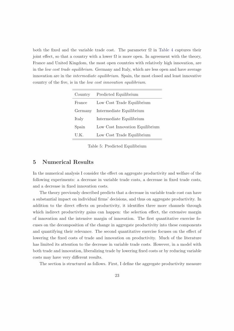
both the fixed and the variable trade cost. The parameter Ω in Table 4 captures their

joint effect, so that a country with a lower Ω is more open. In agreement with the theory,

France and United Kingdom, the most open countries with relatively high innovation, are

in the low cost trade equilibrium. Germany and Italy, which are less open and have average

innovation are in the intermediate equilibrium. Spain, the most closed and least innovative

country of the five, is in the low cost innovation equilibrium.

Country Predicted Equilibrium

France Low Cost Trade Equilibrium

Germany Intermediate Equilibrium

Italy Intermediate Equilibrium

Spain Low Cost Innovation Equilibrium

U.K. Low Cost Trade Equilibrium

Table 5: Predicted Equilibrium

5 Numerical Results

In the numerical analysis I consider the effect on aggregate productivity and welfare of the

following experiments: a decrease in variable trade costs, a decrease in fixed trade costs,

and a decrease in fixed innovation costs.

The theory previously described predicts that a decrease in variable trade cost can have

a substantial impact on individual firms’ decisions, and thus on aggregate productivity. In

addition to the direct effects on productivity, it identifies three more channels through

which indirect productivity gains can happen: the selection effect, the extensive margin

of innovation and the intensive margin of innovation. The first quantitative exercise fo-

cuses on the decomposition of the change in aggregate productivity into these components

and quantifying their relevance. The second quantitative exercise focuses on the effect of

lowering the fixed costs of trade and innovation on productivity. Much of the literature

has limited its attention to the decrease in variable trade costs. However, in a model with

both trade and innovation, liberalizing trade by lowering fixed costs or by reducing variable

costs may have very different results.

The section is structured as follows. First, I define the aggregate productivity measure

23

used in the quantitative exercises, as well as its relation to welfare, following the definition

of Atkeson and Burstein (2010). Second, I decompose changes in aggregate productivity

following a drop in variable trade costs into its different components. Finally, I analyze the

effectiveness of a trade liberalization policy versus the effectiveness of an innovation policy

on aggregate productivity.

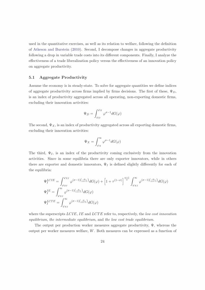
5.1 Aggregate Productivity

Assume the economy is in steady-state. To solve for aggregate quantities we define indices

of aggregate productivity across firms implied by firms decisions. The first of these, ΨD,

is an index of productivity aggregated across all operating, non-exporting domestic firms,

excluding their innovation activities:

ΨD =

∫ ϕX

ϕD

ϕσ−1dG(ϕ)

The second, ΨX , is an index of productivity aggregated across all exporting domestic firms,

excluding their innovation activities:

ΨX =

∫ ∞

ϕX

ϕσ−1dG(ϕ)

The third, ΨI , is an index of the productivity coming exclusively from the innovation

activities. Since in some equilibria there are only exporter innovators, while in others

there are exporter and domestic innovators, ΨI is defined slightly differently for each of

the equilibria:

ΨLCIEI =

∫ ϕXI

ϕDI

ϕ(σ−1)( αα+1)dG(ϕ) +

[1 + τ (1−σ)

]α+1α

∫ ∞

ϕXI

ϕ(σ−1)( αα+1)dG(ϕ)

ΨIEI =

∫ ∞

ϕXI

ϕ(σ−1)( αα+1)dG(ϕ)

ΨLCTEI =

∫ ∞

ϕXI

ϕ(σ−1)( αα+1)dG(ϕ)

where the superscripts LCIE, IE and LCTE refer to, respectively, the low cost innovation

equilibrium, the intermediate equilibrium, and the low cost trade equilibrium.

The output per production worker measures aggregate productivity, Ψ, whereas the

output per worker measures welfare, W . Both measures can be expressed as a function of

24

the productivity indices previously described:

Ψ =Q

Lp=[M(ΨD +

(1 + τ1−σ

)ΨX + F (τ)IΨI

)] 1σ−1 (15)

W =Q

L=

(σ − 1

σ

)[M(ΨD +

(1 + τ1−σ

)ΨX + F (τ)IΨI

)] 1σ−1 (16)

where I is the minimum level of innovation of an innovating firm in each equilibrium, and

F (τ) is a function of the variable trade costs different in each equilibrium. Appendix D

provides a formal derivation of the aggregate productivity in the different equilibria. I

focus on this measure of productivity because it is the measure of productivity that is

relevant for welfare in our model and is similar to the ideal measure of productivity defined

by Atkeson and Burstein (2010), hence making our results comparable.7

5.2 Decomposing the Productivity Effect of a Reduction in Variable

Trade Costs

In this section, I analytically and quantitatively study the impact of a change in marginal

trade costs on the measure of aggregate productivity. Following Atkeson and Burstein

(2010), I do a first order approximation of the effect of a reduction in marginal interna-

tional trade costs τ , decomposing its impact on productivity into a direct effect and an

indirect effect. The direct effect takes all firms’ decisions as given, and simply measures the

productivity gains from trade being less wasteful, whereas the indirect effect arises from

changes in firms’ entry, export and innovation decisions, which are themselves responding

to the change in trade costs. The following proposition shows the decomposition.

Proposition 4. The total change in productivity from a change in trade costs and be

decomposed into a direct effect and an indirect effect. Moreover, the indirect effect can be

7This measure of aggregate productivity does not necessarily correspond to aggregate productivity asmeasured in the data. If all differentiated products are intermediate goods used in production of final goods,changes in the price level for final expenditures can be directly measure using final goods and ΔlogΨ is thevariation of measured productivity. If all different products are consumed directly as final goods, then theproblem of measuring changes in the price level for final expenditures is more complicated. See Atkesonand Burstein (2010) and Bajona et al. (2008) for a discussion of related issues.

25

decomposed into an entry effect, a reallocation effect, and an innovation effect.

ΔlogΨ = −sXΔlog(τ)︸ ︷︷ ︸Exports

−(ΔF (τ)

τ

)sInnIΔlog(τ)︸ ︷︷ ︸

Exporters′ Innovation

⎫⎪⎪⎪⎬⎪⎪⎪⎭Direct

Effect

+ 1σ−1

⎡⎢⎢⎢⎣ Δlog(M)︸ ︷︷ ︸Entry Effect

+ sDΔlog (ΨD)︸ ︷︷ ︸Domestic Market

+

(1 + nτ1−σ

nτ1−σ

)sXΔlog (ΨX)︸ ︷︷ ︸

Export Market

+ sInnIΔlog(I)︸ ︷︷ ︸Extensive Margin

+ sInnIΔlog(ΨI)︸ ︷︷ ︸Intensive Margin

⎤⎥⎦︸ ︷︷ ︸

Innovation

⎫⎪⎪⎪⎪⎪⎪⎪⎪⎪⎪⎪⎪⎪⎬⎪⎪⎪⎪⎪⎪⎪⎪⎪⎪⎪⎪⎪⎭

Indirect

Effect

Proof. Since in each equilibria the decisions on innovation are different, I use a general syn-

tax to point out the different components of the decomposition. The exact equations along

with the full proof are in Appendix D. In what follows, I sketch briefly the mathematics

behind the decomposition 8.

Recall that for every x ∈ RΔx

x= Δlog(x)

Take logs of Ψ

Ψ =1

σ − 1

[log(M) + log

(ΨD +

(1 + τ1−σ

)ΨX + F (τ)IΨI

)]And derivatives

ΔlogΨ =1

σ − 1

[Δlog(M) + ΔlogΨ

]ΔlogΨ =

1

Ψ

[ΔΨD +Δ

(1 + τ1−σ

)ΨX +

(1 + τ1−σ

)ΔΨX

+ΔF (τ)IΨI + F (τ)ΔIΨI + F (τ)IΔΨI ]

Define the share of domestic production excluding innovation in the value of production

8This derivation works well only for infinitesimal changes

26

sD = ΨD

Ψ, the share of export production excluding innovation in the value of production

sX = nτ1−σΨX

Ψand the share of exporters innovation activities in the value of production

sLCIXI =

(1+nτ1−σ)α+1α ΨXI

Ψand sIE,LCT

XI =(1+nτ1−σ)ΨXI

Ψ.

The purpose of the decomposition is to test the prediction of the theoretical model

and to quantify the importance of the different effects. I now discuss each effect, and its

expected theoretical sign. The direct effect takes all firms’ decisions as given and has two

positive components: the first captures the productivity gain of exporters which lose less

output from exporting, and the second captures the additional return from innovation by

exporters that now face lower trade costs. The indirect effect has five components: the

first three correspond to the selection effect described in Melitz (2003), whereas the last

two correspond to the change in innovation. As for the selection effect, the first component

corresponds to a drop in trade costs inducing the exit of less productive firms, implying

the entry effect should be negative. The second and third components have to do with

the reallocation of market shares between the remaining domestic and exporting firms.

Less productive firms lose market share to more productive exporting firms, hence the

domestic indirect effect should be negative and the exporters indirect effect positive. As

for the innovation effect, it can be decomposed into the intensive and extensive margin of

innovation. The innovation intensity increases with the participation in foreign markets

and thus, the effect through the intensive margin of innovation of the exporters innovators

should be positive. For the extensive margin, the theory predicts that the effect can be

positive or negative. In the low cost trade equilibrium and the intermediate equilibrium,

all innovators are exporting. In that case a decrease in iceberg trade costs increases the

incentives to be an exporter (and to be an exporter innovator), so that the effect through the

extensive margin of innovation should be positive. In the low cost innovation equilibrium,

innovation happens by both exporting and domestic firms. Hence, while a decrease in

iceberg trade costs increases the incentives of exporters to innovate, for the domestic firms

innovation becomes harder, as real wages are pushed up. This implies that the productivity

cutoff of domestic innovators moves to the right, so that the effect through the extensive

margin of innovation will be negative.

27

France

Germany

Italy

Spain

United

Kingdom

TotalEffect

0.643

0.642

0.806

0.650

0.597

DirectEffect

0.590

0.593

0.714

1.294

0.560

Exporter

0.021

0.017

0.055

0.031

0.005

Exporters’Innovation

0.569

0.576

0.659

1.263

0.555

IndirectEffect

0.053

0.049

0.092

−0.644

0.038

Entry

−1.182

−1.265

−2.033

−1.555

−1.115

DomesticMarket

−0.010

−0.003

−0.014

−0.006

−0.003

ExportMarket

0.062

0.038

0.167

0.087

0.015

Innovation

1.183

1.279

1.973

0.830

1.141

Extensive

Margin

0.108

0.099

0.089

−0.568

0.065

Intensive

Margin

1.075

1.181

1.884

1.399

1.076

Equilibrium

LCT

IEIE

LCI

LCT

Table

6:ElasticitiesLow

eringIceb

ergTradeCosts1%

28

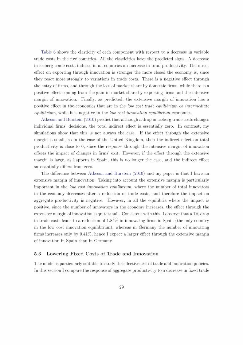
Table 6 shows the elasticity of each component with respect to a decrease in variable

trade costs in the five countries. All the elasticities have the predicted signs. A decrease

in iceberg trade costs induces in all countries an increase in total productivity. The direct

effect on exporting through innovation is stronger the more closed the economy is, since

they react more strongly to variations in trade costs. There is a negative effect through

the entry of firms, and through the loss of market share by domestic firms, while there is a

positive effect coming from the gain in market share by exporting firms and the intensive

margin of innovation. Finally, as predicted, the extensive margin of innovation has a

positive effect in the economies that are in the low cost trade equilibrium or intermediate

equilibrium, while it is negative in the low cost innovation equilibrium economies.

Atkeson and Burstein (2010) predict that although a drop in iceberg trade costs changes

individual firms’ decisions, the total indirect effect is essentially zero. In contrast, my

simulations show that this is not always the case. If the effect through the extensive

margin is small, as in the case of the United Kingdom, then the indirect effect on total

productivity is close to 0, since the response through the intensive margin of innovation

offsets the impact of changes in firms’ exit. However, if the effect through the extensive

margin is large, as happens in Spain, this is no longer the case, and the indirect effect

substantially differs from zero.

The difference between Atkeson and Burstein (2010) and my paper is that I have an

extensive margin of innovation. Taking into account the extensive margin is particularly

important in the low cost innovation equilibrium, where the number of total innovators

in the economy decreases after a reduction of trade costs, and therefore the impact on

aggregate productivity is negative. However, in all the equilibria where the impact is

positive, since the number of innovators in the economy increases, the effect through the

extensive margin of innovation is quite small. Consistent with this, I observe that a 1% drop

in trade costs leads to a reduction of 1.84% in innovating firms in Spain (the only country

in the low cost innovation equilibrium), whereas in Germany the number of innovating

firms increases only by 0.41%, hence I expect a larger effect through the extensive margin

of innovation in Spain than in Germany.

5.3 Lowering Fixed Costs of Trade and Innovation

The model is particularly suitable to study the effectiveness of trade and innovation policies.

In this section I compare the response of aggregate productivity to a decrease in fixed trade

29

costs versus the response to a decrease in fixed innovation costs. While much of the trade

literature focuses on decreases in variable trade costs, evaluating the effect of lowering fixed

costs is also important. This is especially true in model where firms take both export and

innovation decisions.9

First, I will describe the effects of a drop in fixed trade costs and a drop in fixed

innovation costs on the decisions of the firms in the economy. Second, I will quantitatively

assess the elasticity of total productivity, and therefore welfare, to fixed costs. Third, I will

analyze the impact on aggregate productivity of a change in the economies’ equilibrium as

a consequence of a large drop in fixed costs.

5.3.1 Effects on firms’ decisions of a drop in fixed costs

A reduction in fixed trade costs increases the incentives to enter the export market. In the

low cost innovation equilibrium and the intermediate equilibrium this implies that there is

an increase in the firms that export and innovate. In the low cost trade equilibrium it implies

that more firms export but that less firms export and innovate. In this equilibrium, the

firms choosing whether to innovate or not are already exporting (and therefore are paying

the fixed export costs), so they only care about innovation costs and variable trade costs.

For them a drop in fixed trade costs lowers the incentives to innovate, since it induces

more entry into the industry, reducing the price index and lowering the profits coming

from innovation. In the next proposition I prove this latter result.

Proposition 5. In the low cost trade equilibrium, if fixed trade costs fall

1. The domestic cutoff increases ∂ϕD/∂fX < 0

2. The productivity cutoff for exporting decreases ∂ϕX/∂fX > 0

3. The productivity cutoff for exporting and innovation increases ∂ϕXI/∂fX < 0

Proof. Assume that G(ϕ) = 1 −(

1ϕ

)θ. Differentiating (Equation B.2) with respect to

fX and using ∂ϕX/∂fX = (ϕX/ϕD) ∂ϕD/∂fX + [1/(σ − 1)]ϕX/fX and ∂ϕXI/∂fX =

(ϕXI/ϕD) ∂ϕD/∂fX from Equation 8, Equation 9 and Equation 10 yields:

9In a pure trade model, without innovation, lowering variable or fixed costs tend to have qualitativelysimilar results on welfare. See (Melitz, 2003) for a more comprehensive explanation.

30

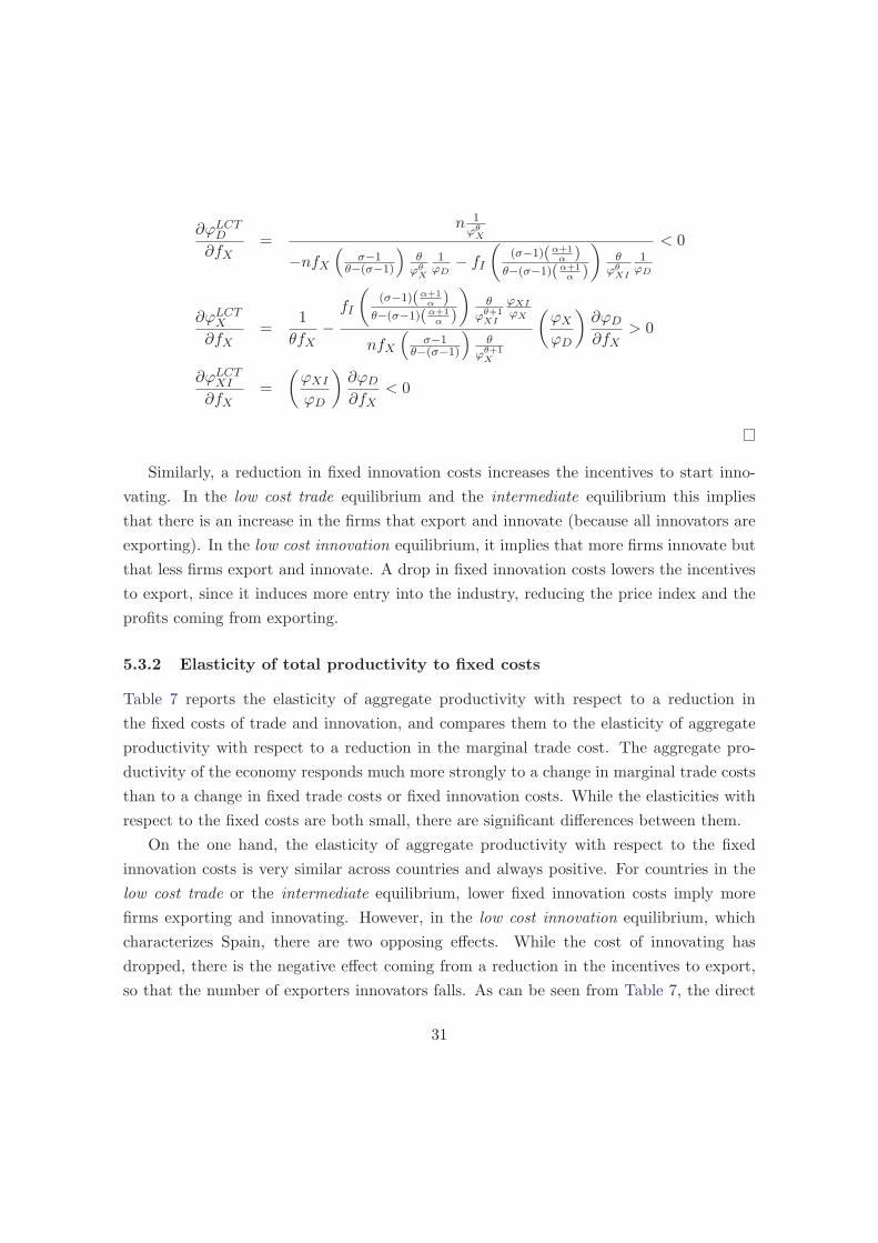
∂ϕLCTD

∂fX=

n 1ϕθX

−nfX

(σ−1

θ−(σ−1)

)θ

ϕθX

1ϕD

− fI

((σ−1)(α+1

α )θ−(σ−1)(α+1

α )

)θ

ϕθXI

1ϕD

< 0

∂ϕLCTX

∂fX=

1

θfX−

fI

((σ−1)(α+1

α )θ−(σ−1)(α+1

α )

)θ

ϕθ+1XI

ϕXIϕX

nfX

(σ−1

θ−(σ−1)

)θ

ϕθ+1X

(ϕX

ϕD

)∂ϕD

∂fX> 0

∂ϕLCTXI

∂fX=

(ϕXI

ϕD

)∂ϕD

∂fX< 0

Similarly, a reduction in fixed innovation costs increases the incentives to start inno-

vating. In the low cost trade equilibrium and the intermediate equilibrium this implies

that there is an increase in the firms that export and innovate (because all innovators are

exporting). In the low cost innovation equilibrium, it implies that more firms innovate but

that less firms export and innovate. A drop in fixed innovation costs lowers the incentives

to export, since it induces more entry into the industry, reducing the price index and the

profits coming from exporting.

5.3.2 Elasticity of total productivity to fixed costs

Table 7 reports the elasticity of aggregate productivity with respect to a reduction in

the fixed costs of trade and innovation, and compares them to the elasticity of aggregate

productivity with respect to a reduction in the marginal trade cost. The aggregate pro-

ductivity of the economy responds much more strongly to a change in marginal trade costs

than to a change in fixed trade costs or fixed innovation costs. While the elasticities with

respect to the fixed costs are both small, there are significant differences between them.

On the one hand, the elasticity of aggregate productivity with respect to the fixed

innovation costs is very similar across countries and always positive. For countries in the

low cost trade or the intermediate equilibrium, lower fixed innovation costs imply more

firms exporting and innovating. However, in the low cost innovation equilibrium, which

characterizes Spain, there are two opposing effects. While the cost of innovating has

dropped, there is the negative effect coming from a reduction in the incentives to export,

so that the number of exporters innovators falls. As can be seen from Table 7, the direct

31

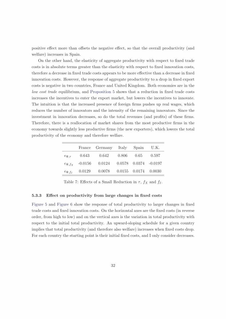
positive effect more than offsets the negative effect, so that the overall productivity (and

welfare) increases in Spain.

On the other hand, the elasticity of aggregate productivity with respect to fixed trade

costs is in absolute terms greater than the elasticity with respect to fixed innovation costs,

therefore a decrease in fixed trade costs appears to be more effective than a decrease in fixed

innovation costs. However, the response of aggregate productivity to a drop in fixed export

costs is negative in two countries, France and United Kingdom. Both economies are in the

low cost trade equilibrium, and Proposition 5 shows that a reduction in fixed trade costs

increases the incentives to enter the export market, but lowers the incentives to innovate.

The intuition is that the increased presence of foreign firms pushes up real wages, which

reduces the number of innovators and the intensity of the remaining innovators. Since the

investment in innovation decreases, so do the total revenues (and profits) of these firms.

Therefore, there is a reallocation of market shares from the most productive firms in the

economy towards slightly less productive firms (the new exporters), which lowers the total

productivity of the economy and therefore welfare.

France Germany Italy Spain U.K.

εΨ,τ 0.643 0.642 0.806 0.65 0.597

εΨ,fX -0.0156 0.0124 0.0578 0.0374 -0.0197

εΨ,fI 0.0129 0.0078 0.0155 0.0174 0.0030

Table 7: Effects of a Small Reduction in τ , fX and fI .

5.3.3 Effect on productivity from large changes in fixed costs

Figure 5 and Figure 6 show the response of total productivity to larger changes in fixed

trade costs and fixed innovation costs. On the horizontal axes are the fixed costs (in reverse

order, from high to low) and on the vertical axes is the variation in total productivity with

respect to the initial total productivity. An upward-sloping schedule for a given country

implies that total productivity (and therefore also welfare) increases when fixed costs drop.

For each country the starting point is their initial fixed costs, and I only consider decreases.

32

05

1015

20Δ

Tot

al P

rodu

ctiv

ity (

ΔΨ

/ Ψ

)

02468 Fixed Trade Costs (fX)

FranceGermanyItalySpainUK

Figure 5: Change in Total Productivity and Fixed Trade Costs

−8

−6

−4

−2

02

ΔT

otal

Pro

duct

ivity

(Δ

Ψ /

Ψ)

0246810 Fixed Innovation Costs (fI)

FranceGermanyItalySpainUK

Figure 6: Change in Total Productivity and Fixed Innovation Costs

33

Several facts stand out in these two figures. First, the response of productivity to

changes in fixed trade costs is stronger than the response to changes in fixed innovation

costs. Second, if the economy is in the low cost trade equilibrium, the total productivity

decreases as fixed trade costs decrease. This is the case of France and the UK. Third, if

fixed innovation costs decrease, total productivity increases the most if the economy is the

low cost innovation equilibrium. This the case of Spain. These three facts are similar to

the ones found when computing the elasticities in Table 7.

However, the figures also reveal that the largest changes in productivity happen when

countries move from one equilibrium to another as a consequence of the drop in fixed

costs. This is especially relevant if the movement from one equilibrium to another has a

big impact on the number of firms in the economy. These changes in productivity can be

positive or negative, large or small, therefore studying what drives them is important to

be able to asses the effectiveness of innovation policies and trade policies.

If the fixed trade cost drops sufficiently, Spain goes from the low cost innovation equi-

librium to the intermediate equilibrium. In Figure 5 this change in equilibrium shows up

as a large upward spike. In this transition 8% of the firms in the economy exit. This

negative effect is more than compensated by an increase of 29% in the productivity of the

economy when ignoring changes on the entry of firms. The large productivity increase is

due to domestic innovators becoming exporting innovators thanks to the increased ease of

entering the export market.

Similarly, if the fixed cost of innovation drops sufficiently, Italy and Germany also

change equilibrium, this time in the other direction, from the intermediate equilibrium to

the low cost innovation equilibrium. Once again, this shows up as a large spike in Figure 6.

Since trade becomes relatively more expensive, after the transition there are less exporter

innovators and more firms enter in the domestic market. The loss through the exporter

innovators dominates the entry of more firms in the economy, hence the spike down in

both economies during the change. Finally, notice that once in the the low cost innovation

equilibrium, the total productivity starts increasing again.

But there are other shifts in equilibria. For example, if the fixed trade cost drops suffi-

ciently, Germany goes from the intermediate equilibrium to the low cost trade equilibrium.

And if the fixed cost of innovation drops sufficiently, France and United Kingdom go from

the low cost trade equilibrium to the intermediate equilibrium. In all these cases, the change

between equilibria is smooth and only the slopes change. In Figure 5, when Germany tran-

sitions to the low cost trade equilibrium, the trend becomes negative, although there are

34

still gains in productivity with respect to the initial productivity since it is now in a more

open economy. The negative effect is consistent with Proposition 5, where a decrease in

fixed trade costs induces losses both through the extensive and the intensive margins of

innovation. Note that France and the United Kingdom, which are already in the low cost

trade equilibrium, display a similar behavior, whereby a drop in fixed trade costs lowers

total productivity. However, since both of them are already in a very export oriented eco-

nomy, there are no gains with respect to the initial productivity, and the decrease translates

in a drop in productivity.

If we turn to the opposite case, going from the low cost trade equilibrium to the in-

termediate equilibrium, as France and United Kingdom do in Figure 6, we see that both

countries react differently. While there is an increase of total productivity in France with

respect to the initial situation, in the United Kingdom the trend is negative and if fixed

innovation costs are low enough, the total productivity decreases with respect to the ini-

tial situation. The decrease in fixed innovation costs induces firms to become exporters

innovators, increasing the market shares of these firms while the most inefficient exit the

economy. While in France the positive effect through the reallocation of market shares

towards the more efficient firms dominates the negative effect through the exit of firms, in

the United Kingdom it is the negative effect through the exit of firms which dominates.

Summarizing, Figure 5 and Figure 6 reveal that a drop in fixed trade costs is more effec-

tive in raising productivity (and welfare) than a drop in fixed innovation costs. Depending

on the country, it can induce productivity gains from 1% to 20% in total, and only if the

economy is already very open might a further drop in fixed trade costs be damaging to the

economy. In contrast, a fixed innovation cost drop has little effect on the productivity, the

maximum increase being around 2%, and if it induces economies to be less export oriented,

then the productivity might decrease by upto 7%.

6 Conclusions

This paper has proposed a trade model with heterogeneous firms that decide not just

whether or how much to export but also whether or how much to innovate. By incorporat-

ing the extensive and intensive margins of trade and innovation, three equilibria may arise.

In all equilibria high-productivity firms export and innovate, whereas low-productivity

neither export nor innovate. What differs across equilibria is the behavior of medium-

productivity firms. In an economy with trade costs that are low relative to innovation costs,

35

medium-productivity firms export without innovating, whereas in an economy with trade

costs that are high relative to innovation costs, medium-productivity firms innovate with-

out exporting. In a third equilibrium, in between the other two, some medium-productivity

firms export and innovate, whereas others do neither.

After characterizing these different equilibria, we have shown that they are empirically

plausible by calibrating the model to five European countries. The numerical exercises

reveal the importance of considering both the intensive and extensive margin of innovation

to understand the interdependence between trade and innovation. More generally, the effect

of trade liberalization on productivity and welfare depends crucially on the equilibrium the

economy is in. A standard result in the literature is that the aggregate productivity effect of

a drop in variable trade costs on firms’ decisions to exit, export and innovate is minimal. In

our setup this is also true in most equilibria, but not in the low cost innovation equilibrium.

In that case a drop in variable trade costs has a negative impact on the extensive margin

of innovation, thus lowering the overall positive effect of trade liberalization.

In addition to analyzing a drop in variable trade costs, I also assessed the impact of

a drop in fixed trade costs and fixed innovation costs. Once again, although in most

equilibria these policies lead to an improvement in aggregate productivity and welfare, this

is not always the case. For example, in the low cost trade equilibrium, a drop in fixed trade

costs increases the number of exporters, making innovating more expensive. This lowers

both the number of innovators and the intensity of innovation, leading to a reduction in

aggregate productivity and welfare.

These findings stress the importance of having a model that jointly analyzes the ex-

tensive and intensive margins of both trade and innovation. Not doing so would not just

result in a less rich theoretical structure, it would also keep us from correctly assessing the

impact of different policies aimed at fomenting trade and innovation.

Of course, this model has abstracted from a number of potentially relevant features

that go beyond the scope of this paper. First, I have exclusively focused on a steady state

environment, thus ignoring the transition dynamics. As shown by Alessandria and Choi

(2011) and Burstein and Melitz (2011), not taking into account transition dynamics may

significantly impact the welfare effects of trade liberalization. Second, the model does not

consider uncertainty in innovation. While most of the literature on trade and innovation

assumes there is no risk involved,10 the empirical evidence suggests otherwise: there is

10An exception is Atkeson and Burstein (2010) who introduce uncertainty in the outcome of the invest-ment in process innovation, although firms always get some returns (no innovation fails).

36

risk that an innovator will not identify important needs, that innovation teams disrupt

the regular operations of a business, or that even a promising idea is not accepted by the

customers whose need it was meant to address. Third, I have assumed that there is no

strategic interaction between firms and therefore the innovation activities of one firm do

not have any influence in the innovation activities of the other firms. The existence of

externalities in process innovation could have a significant effect on the results. Fourth,

the model could be used to analyze the effect of joint trade and innovation policies. The

right mix of policies could lead to greater gains in aggregate productivity.

37

References

Alessandria, G. and H. Choi (2011). Establishment heterogeneity, exporter dynamics,

and the effects of trade liberalization. Working Papers 11-19, Federal Reserve Bank of

Philadelphia.

Arkolakis, C., A. Costinot, and A. Rodriguez-Clare (2012). New trade models, same old

gains? American Economic Review 102 (1), 94–130.

Atkeson, A. and A. T. Burstein (2010). Innovation, Firm Dynamics, and International

Trade. Journal of Political Economy 118 (3), pp. 433–484.

Bajona, C., M. J. Gibson, T. J. Kehoe, and K. J. R. and (2008). Trade liberalization growth

and productivity. 2008 Meeting Papers 789, Federal Reserve Bank of Minneapolis.

Baldwin, R. E. and F. Robert-Nicoud (2008). Trade and growth with heterogeneous firms.

Journal of International Economics 74 (1), 21–34.

Bernard, A. B., S. J. Redding, and P. K. Schott (2007). Comparative Advantage and

Heterogeneous Firms. Review of Economic Studies 74 (1), 31–66.

Broda, C. and D. E. Weinstein (2006). Globalization and the Gains from Variety. The

Quarterly Journal of Economics 121 (2), 541–585.

Burstein, A. and M. J. Melitz (2011). Trade liberalization and firm dynamics. NBER

Working Papers 16960, National Bureau of Economic Research, Inc.

Bustos, P. (2011). Trade Liberalization, Exports, and Technology Upgrading: Evidence on

the Impact of MERCOSUR on Argentinian Firms. American Economic Review 101 (1),

304–40.

Chaney, T. (2008). Distorted gravity: The intensive and extensive margins of international

trade. American Economic Review 98 (4), 1707–21.

Costantini, J. A. and M. J. Melitz (2008). The Organization of Firms in a global economy,

Chapter The Dynamics of Firm Level Adjustment to Trade Liberalization. Harvard

University Press.

Crespo, A. (2011). Trade and Innovation: Extensive and Intensive Margin. mimeo.

38

Griliches, Z. (1979). Issues in assessing the contribution of research and development to

productivity growth. Bell Journal of Economics 10 (1), 92–116.

Helpman, E., M. J. Melitz, and S. R. Yeaple (2004). Export versus fdi with heterogeneous

firms. American Economic Review 94 (1), 300–316.

Klette, T. J. and S. Kortum (2004). Innovating Firms and Aggregate Innovation. Journal

of Political Economy 112 (5), 986–1018.

Krugman, P. (1980). Scale economies, product differentiation, and the pattern of trade.

American Economic Review 70 (5), 950–59.

Lentz, R. and D. T. Mortensen (2008). An Empirical Model of Growth through Product

Innovation. Econometrica 76 (6), 1317–1373.

Melitz, M. J. (2003). The Impact of Trade on Intra-Industry Reallocations and Aggregate

Industry Productivity. Econometrica 71 (6), 1695–1725.

Navas-Ruiz, A. and D. Sala (2007). Technology adoption and the selection effect of trade.

Open access publications from universidad carlos iii de madrid, Universidad Carlos III

de Madrid.

Rubini, L. (2011). Innovation and the elasticity of trade volumes to tariff reductions.

MPRA Paper 21484, EFIGE Working Paper 31.

Stahler, F., H. Raff, and N. Van Long (2007). The Effects of Trade Liberalization on

Productivity and Welfare: The Role of Firm Heterogeneity, R&D and Market Struc-

ture. Economics working papers, Christian-Albrechts-University of Kiel, Department of

Economics.

Vannoorenberghe, G. (2008). Globalization, heterogeneous firms and endogenous invest-

ment. mimeo.

Vives, X. (2008). Innovation and competitive pressure. The Journal of Industrial Eco-

nomics 56 (3), pp. 419–469.

Yeaple, S. R. (2005). A simple model of firm heterogeneity, international trade, and wages.

Journal of International Economics 65 (1), 1–20.

39

Appendix A - Low Cost Innovation Economy

Productivity distribution and weighted averages

Let us denote by μD (ϕ), μDI (ϕ) and μXI (ϕ) respectively, the productivity distribu-

tion of domestic producers, active innovators and active innovators and exporters prior to

innovation.

μD (ϕ) =

{g(ϕ)

G(ϕDI)−G(ϕD) , ϕDI > ϕ ≥ ϕD

0 , otherwise

μDI (ϕ) =

{g(ϕ)

G(ϕXI)−G(ϕDI), ϕXI ≥ ϕ ≥ ϕDI

0 , otherwise

μXI (ϕ) =

{g(ϕ)

1−G(ϕXI), ϕ ≥ ϕXI

0 , otherwise

The distributions μD (ϕ), μDI (ϕ) and μXI (ϕ) are not affected by the simultaneous

entry and exit since the successful entrants and failing incumbents draw their productivity

level from the common distribution μ (ϕ) .

Let ϕ =[∫∞

ϕDϕσ−1μ (ϕ) dϕ

] 1(σ−1)

and ϕX =[∫∞

ϕXIϕσ−1μXI (ϕ) dϕ

] 1(σ−1)

denote the

average productivity levels of, respectively, all firms and exporting firms only prior to

innovation. Then the weighted productivity average that reflects the combined market

share of all firms can be defined as

ϕt =

{1

Mt

[Mϕσ−1 + nMX

(τ−1ϕX

)σ−1]} 1

σ−1

And let ϕDI =

[∫∞ϕDI

(ϕσ−1

) (α+1)α μDI (ϕ) dϕ

] α(α+1)

1(σ−1)

and ϕXI represent the average

productivity the domestic innovators and exporter innovators get from innovation. Thenthe weighted productivity average that reflects the combined market share of innovationcan be defined as

ϕIt =

{1

MIt

[MI (ϕDI)

(σ−1)(α+1α ) +mXI

((1 + nτ1−σ)α+1

α − 1

)(ϕXI)

(σ−1)(α+1α )

]}( αα+1 )(

1σ−1 )

40

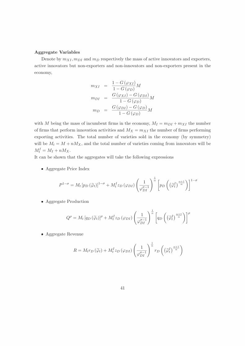
Aggregate Variables

Denote by mXI ,mDI and mD respectively the mass of active innovators and exporters,

active innovators but non-exporters and non-innovators and non-exporters present in the

economy,

mXI =1−G (ϕXI)

1−G (ϕD)M

mDI =G (ϕXI)−G (ϕDI)

1−G (ϕD)M

mD =G (ϕDI)−G (ϕD)

1−G (ϕD)M

with M being the mass of incumbent firms in the economy, MI = mDI +mXI the number

of firms that perform innovation activities and MX = mXI the number of firms performing

exporting activities. The total number of varieties sold in the economy (by symmetry)

will be Mt = M + nMX , and the total number of varieties coming from innovators will be

M It = MI + nMX .

It can be shown that the aggregates will take the following expressions

� Aggregate Price Index

P 1−σ = Mt [pD (ϕt)]1−σ +M I

t zD (ϕDI)

(1

ϕσ−1DI

) 1α [

pD

((ϕIt

)α+1α

)]1−σ

� Aggregate Production

Qρ = Mt [qD (ϕt)]ρ +M I

t zD (ϕDI)

(1

ϕσ−1DI

) 1α [

qD

((ϕIt

)α+1α

)]ρ

� Aggregate Revenue

R = MtrD (ϕt) +M It zD (ϕDI)

(1

ϕσ−1DI

) 1α

rD

((ϕIt

)α+1α

)

41

� Aggregate Profits

Π = MtrD (ϕt)

σ−MfD − nMXfX −MIfI +MIα

(1

α+ 1

)α+1α(rD (ϕI)

σ

)α+1α

+mXI

[(1 + nτ1−σ

)α+1α − 1

]α

(1

α+ 1

)α+1α(rD (ϕXI)

σ

)α+1α

(A.1)

Low Cost Innovation Equilibrium

Proof of Proposition 1, part II

If there are sufficiently high fixed export cost, there exist a single cutoff ϕ∗XI that solves

equation (6)

Proof. The proof is divided in three sections

First, I show that the LHS of equation (6) is positive with respect to the productivity

parameter. πXI (ϕXI)− πDI (ϕXI) ≥ 0

[(1 + nτ1−σ

)α+1α − 1

]α(

1α+1

)α+1α[(

R(Pρ)σ−1

σ

)ϕσ−1

]α+1α

+nτ1−σ(R(Pρ)σ−1

σ

)ϕσ−1−nfx≥ 0

C1

(ϕσ−1

)α+1α + C2ϕ

σ−1 − nfx ≥ 0

∂LHS

∂ϕ= C1

(α+ 1

α

)(σ − 1)ϕ(

α+1α )(σ−1)−1 + C2 (σ − 1)ϕσ−2 > 0

Secondly, I show that πXI (ϕDI) − πDI (ϕDI) < 0, otherwise the firm would choose to

export and innovate instead of being indifferent between innovating or not while staying

in the domestic market.

πXI (ϕDI)− πDI (ϕDI) < 0[(1 + nτ1−σ

)α+1α − 1

]fI + nτ1−σ

(fIα

) αα+1

(α+ 1)− nfX < 0

Thus, for fX large enough, that is for

fX >

[(1 + nτ1−σ

)α+1α − 1

]fIn

+ τ1−σ

(fIα

) αα+1

(α+ 1)

it holds that πXI (ϕDI)− πDI (ϕDI) < 0

42

Finally, I show that the difference between the profits of the exporting and non-

exporting strategies while innovation goes to infinite as the productivity of the firm is

larger.

If ϕ → ∞,then πXI (zD (ϕ)) − πDI (zD (ϕ)) → ∞, since by definition πXI (zX (ϕ)) >

πXI (zD (ϕ)) then it must be that πXI (zX (ϕ))− πDI (zD (ϕ)) → ∞ as ϕ → ∞

πXI (zD (ϕ))− πDI (zD (ϕ)) = nτ1−σ [1 + z]

(R (Pρ)σ−1

σ

)ϕσ−1 − nfX

= nτ1−σ

(1

α+ 1

) 1α

[(R (Pρ)σ−1

σ

)ϕσ−1

]α+1α

+nτ1−σ

(R (Pρ)σ−1

σ

)ϕσ−1 − nfX

limϕ→∞ [πXI (zD (ϕ))− πDI (zD (ϕ))] = lim

ϕ→∞

[C4

[ϕσ−1

]α+1α + C5ϕ

σ−1 − C6

]= lim

ϕ→∞

[C4

[ϕσ−1

]α+1α

]+ lim

ϕ→∞[C5ϕ

σ−1]− lim

ϕ→∞ (C6) → ∞

Proof of Proposition 1, part I

Equations (4) to (6) along with the Free Entry condition (7) completely determine

the equilibrium and the productivity cutoffs can be uniquely determined and allow me to

rearrange the FE conveniently for the characterizing of the equilibrium as a function of ϕ∗D

δfE = [1−G (ϕ∗D)]π

δfE = fDj1 (ϕ∗D) + nτ1−σfDj2 (ϕ

∗X (ϕ∗

D))− [1−G (ϕ∗XI)]nfX (A.2)

− [1−G (ϕ∗DI)] fI + α

(1

α+ 1

)α+1α

fα+1α

D j3 (ϕ∗D)

+α

(1

α+ 1

)α+1α

fDα+1α

[(1 + nτ1−σ

)α+1α − 1

]j4 (ϕ

∗D)

43

where j1 (ϕ∗D) =

[(ϕ (ϕ∗

D) /ϕ∗D)

σ−1 − 1], j2 (ϕ

∗D) = (ϕx (ϕ

∗D) /ϕ

∗D)

σ−1 [1−G (ϕ∗XI)]

j3 (ϕ∗D) =

[(ϕDI (ϕ

∗D) /ϕ

∗D)

σ−1]α+1

α[1−G (ϕ∗

DI)] and

j4 (ϕ∗D) =

[(ϕXI (ϕ

∗D) /ϕ

∗D)

σ−1]α+1

α[1−G (ϕ∗

XI)]

Proof.

Assume the parameter restrictions τσ−1fX ≥[(1+nτ1−σ)

α+1α −1

]

nτ1−σ fI +(fIα

) αα+1

(α+ 1) and(fIα

) αα+1

(α+ 1) ≥ fD hold, then the Low Cost Innovation Equilibrium exists and is unique.

I shall proof that the RHS of equation (A.2) is decreasing in ϕ∗D on the domain (ϕ∗

D,∞),

so that ϕ∗D is uniquely determined by the intersection of the latter curve with the flat line

δfE in the (ϕ∗D,∞) space.

Let k1 (ϕ∗D) =

[(ϕ (ϕ∗

D) /ϕ∗D)

σ−1 − 1], then

k′1 (ϕ∗D) =

g (ϕ∗D)

1−G(ϕ∗D

)k1 (ϕ∗D)−

(σ − 1) [k1 (ϕ∗D) + 1]

ϕ∗D

Similarly, k3 (ϕ∗D) =

[(ϕDI (ϕ

∗D) /ϕ

∗D)

σ−1]α+1

α, thus

k′3 (ϕ∗D) = Λ

1σ−1

g (ϕ∗I)

1−G(ϕ∗I

) [k2 (ϕ∗D)− Λ

α+1α

]−(α+ 1

α

)(σ − 1)

k2 (ϕ∗D)

ϕ∗D

where∂ϕ∗

DI∂ϕ∗

D=

[(fIα

) αα+1 (α+1)

fD

] 1σ−1

= Λ1

σ−1

Now, define j1 (ϕ∗D) = [1−G (ϕ∗

D)] k1 (ϕ∗D) , and j3 (ϕ

∗D) = [1−G (ϕ∗

DI)] k3 (ϕ∗D) which are

non-negative.

Then the derivative and elasticity of j1 (ϕ∗D) and j3 (ϕ

∗D) are

j′1 (ϕ∗D) = −(σ − 1) [k1 (ϕ

∗D) + 1]

ϕ∗D

[1−G (ϕ∗D)] < 0

j′1 (ϕ∗D) · ϕ∗

D

j1(ϕ∗D

) = − (σ − 1)

[1 +

1

k1(ϕ∗D

)]︸ ︷︷ ︸<0 and bounded away of it

< − (σ − 1)

44

and

j′3 (ϕ∗D) = −g (ϕ∗

DI) Λ1

σ−1Λ

α+1α − θ (α+ 1) (σ − 1)

k3 (ϕ∗D)

ϕ∗D

[1−G (ϕ∗DI)] < 0

j′3 (ϕ∗D) · ϕ∗

D

j3(ϕ∗D

) = − g (ϕ∗DI)[

1−G(ϕ∗DI

)] Λ 1σ−1

Λα+1α

k2(ϕ∗D

) ϕ∗D − β (σ − 1)︸ ︷︷ ︸

<0 and bounded away of it

< −β (σ − 1)

Thus, j1 (ϕ∗D) and j3 (ϕ

∗D) must be decreasing to zero as ϕ goes to infinite. Furthermore,

it must be that limϕ∗D→0

j1 (ϕ∗D) = ∞ since lim

ϕ∗D→0

k1 (ϕ∗D) = ∞.and lim

ϕ∗D→0

j3 (ϕ∗D) = ∞ since

limϕ∗D→0

k3 (ϕ∗D) = ∞

Since j1 (ϕ∗D) and j3 (ϕ

∗D), it follows that j2 (ϕ

∗D) and j4 (ϕ

∗D) do also monotonically decrease

from infinite to zero on the (0,∞) parameter space.

Therefore, the RHS of (A.2) is a monotonic decreasing function from infinity to zero

on the space (0,∞) that cuts the FE flat line from above identifying a unique cutoff level

ϕ∗D.

45

Appendix B - Low Cost Trade Economy

Productivity distribution and weighted averages

Let us denote by μD (ϕ), μX (ϕ) and μXI (ϕ) respectively, the productivity distribution

of domestic producers, exporters and innovators exporters.

μD (ϕ) =

{g(ϕ)

G(ϕX)−G(ϕD) , ϕX > ϕ ≥ ϕD

0 , otherwise

μX (ϕ) =

{g(ϕ)

G(ϕXI)−G(ϕX) , ϕXI ≥ ϕ ≥ ϕX

0 , otherwise

μXI (ϕ) =

{g(ϕ)

1−G(ϕXI), ϕ ≥ ϕXI

0 , otherwise

The distributions μD (ϕ), μX (ϕ) and μXI (ϕ) are not affected by the simultaneous

entry and exit since the successful entrants and failing incumbents draw their productivity

level from the common distribution μ (ϕ) .

Let ϕ =[∫∞

ϕDϕσ−1μ (ϕ) dϕ

] 1(σ−1)

and ϕX =[∫∞

ϕXIϕσ−1μXI (ϕ) dϕ

] 1(σ−1)

denote the

average productivity levels of, respectively, all firms and exporting firms only prior to

innovation. Then the weighted productivity average that reflects the combined market

share of all firms can be defined as

ϕt =

{1

Mt

[Mϕσ−1 + nMX

(τ−1ϕX

)σ−1]} 1

σ−1

And let ϕXI =

[∫∞ϕXI

(ϕσ−1

) (α+1)α μXI (ϕ) dϕ

] α(α+1)

1(σ−1)

represent the average productivity

the innovators get from innovation.

Aggregate Variables

Denote by mXI ,mX and mD respectively the mass of active innovators and exporters,

only exporters and non-innovators non-exporters present in the economy,

mXI =1−G (ϕXI)

1−G (ϕD)M

mX =G (ϕXI)−G (ϕX)

1−G (ϕD)M

46

mD =G (ϕX)−G (ϕD)

1−G (ϕD)M

with M being the mass of incumbent firms in the economy, MI = mXI the number of firms

that perform innovation activities and MX = mX +mXI the number of firms performing

exporting activities. The total number of varieties sold in the economy (by symmetry) will

be Mt = M + nMX .

It can be shown that the aggregates will take the following expressions

� Aggregate Price Index

P 1−σ = Mt [pD (ϕt)]1−σ

+mXI

(1 + nτ1−σ

)zX (ϕXI)

(1

ϕσ−1XI

) 1α[pD

(ϕ(α+1

α )XI

)]1−σ

� Aggregate Production

Qρ = Mt [qD (ϕt)]ρ +mXI

(1 + nτ1−σ

)zX (ϕXI)

(1

ϕσ−1XI

) 1α [

qD

(ϕ(α+1

α )XI

)]ρ

� Aggregate Revenue

R = MtrD (ϕt) +mXI

(1 + nτ1−σ

)zX (ϕXI)

(1

ϕσ−1XI

) 1α

rD

(ϕ(α+1

α )XI

)

� Aggregate Profits

Π = MtrD (ϕt)

σ−MfD − nMXfX −mXIfI (B.1)

+mXI

(1 + nτ1−σ

)α

(1

α+ 1

)α+1α(rD (ϕI)

σ

)α+1α

Low Cost Trade Economy Equilibrium

Proof of Proposition 2

Equations (8) to (10) along with the Free Entry condition (11)completely determine the

equilibrium and the productivity cutoffs can be uniquely determined and I can rearrange

the FE conveniently for the characterizing of the equilibrium as a function of ϕ∗D

47

δfE = [1−G (ϕ∗D)]π

δfE = fDl1 (ϕ∗D) + nfX l2 (ϕ

∗X (ϕ∗

D)) (B.2)

+α

(1

α+ 1

)α+1α [

fD(1 + τ1−σ

)](α+1α )

l3 (ϕ∗D)− [1−G (ϕ∗

XI)] fI

where j1 (ϕ∗D) =

[(ϕ (ϕ∗

D) /ϕ∗D)

σ−1 − 1], j2 (ϕ

∗X (ϕ∗

D)) =[(ϕ (ϕ∗

X) /ϕ∗X)σ−1 − 1

][1−G (ϕ∗

X)]

and j3 (ϕ∗D) =

[(ϕXI (ϕ

∗D) /ϕ

∗D)

σ−1](α+1

α )[1−G (ϕ∗

XI)]

Proof.

Assume the parameter restriction

(fIα

) αα+1

(α+1)

(1+nτ1−σ)≥ τσ−1fX ≥ fD holds, then the Low Cost

Trade Equilibrium exists and is unique. I shall proof that the RHS of equation (B.2)

is decreasing in ϕ∗D on the domain (ϕ∗

D,∞), so that ϕ∗D is uniquely determined by the

intersection of the latter curve with the flat line δfE in the (ϕ∗D,∞) space.

Let k1 (ϕ∗D) =

[(ϕ (ϕ∗

D) /ϕ∗D)

σ−1 − 1], then

k′1 (ϕ∗D) =

g (ϕ∗D)

1−G(ϕ∗D

)k1 (ϕ∗D)−

(σ − 1) [k1 (ϕ∗D) + 1]

ϕ∗D

Similarly, k3 (ϕ∗D) =

[(ϕDI (ϕ

∗D) /ϕ

∗D)

σ−1]α+1

α, thus

k′3 (ϕ∗D) = Λ

1σ−1

g (ϕ∗I)

1−G(ϕ∗I

) [k2 (ϕ∗D)− Λ

α+1α

]−(α+ 1

α

)(σ − 1)

k2 (ϕ∗D)

ϕ∗D

where∂ϕ∗

DI∂ϕ∗

D=

[(fIα

) αα+1 (α+1)

fD

] 1σ−1

= Λ1

σ−1

Now, define j1 (ϕ∗D) = [1−G (ϕ∗

D)] k1 (ϕ∗D) , and j2 (ϕ

∗D) = [1−G (ϕ∗

DI)] k2 (ϕ∗D) which are

non-negative.

Then the derivative and elasticity of j1 (ϕ∗D) and j3 (ϕ

∗D) are

j′1 (ϕ∗D) = −(σ − 1) [k1 (ϕ

∗D) + 1]

ϕ∗D

[1−G (ϕ∗D)] < 0

48

j′1 (ϕ∗D) · ϕ∗

D

j1(ϕ∗D

) = − (σ − 1)

[1 +

1

k1(ϕ∗D

)]︸ ︷︷ ︸<0 and bounded away of it

< − (σ − 1)

and

j′3 (ϕ∗D) = −g (ϕ∗

DI) Λ1

σ−1Λ

α+1α − θ (α+ 1) (σ − 1)

k3 (ϕ∗D)

ϕ∗D

[1−G (ϕ∗DI)] < 0

j′3 (ϕ∗D) · ϕ∗

D

j3(ϕ∗D

) = − g (ϕ∗DI)[

1−G(ϕ∗DI

)] Λ 1σ−1

Λα+1α

k2(ϕ∗D

) ϕ∗D − β (σ − 1)︸ ︷︷ ︸

<0 and bounded away of it

< −β (σ − 1)

Thus, j1 (ϕ∗D) and j3 (ϕ

∗D) must be decreasing to zero as ϕ goes to infinite. Further-

more, it must be that limϕ∗D→0

j1 (ϕ∗D) = ∞ since lim

ϕ∗D→0

k1 (ϕ∗D) = ∞ and lim

ϕ∗D→0

j3 (ϕ∗D) = ∞

since limϕ∗D→0

k3 (ϕ∗D) = ∞. Since j1 (ϕ

∗D) and j3 (ϕ

∗D) are decreasing from infinity to zero on

(0,∞),from the closed economy case, it follows that j2 (ϕ∗X (ϕ∗

D)) does also monotonically

decrease from infinite to zero on the (0,∞) parameter space.

Therefore, the RHS of (B.2) is a monotonic decreasing function from infinity to zero

on the space (0,∞) that cuts the FE flat line from above identifying a unique cutoff level

ϕ∗D.

49

Appendix C - Intermediate Economy

Productivity distribution and weighted averages

Let us denote by μD (ϕ), and μXI (ϕ) respectively, the productivity distribution of

domestic producers, and active innovators and exporters prior to innovation.

μD (ϕ) =

{g(ϕ)

G(ϕXI)−G(ϕD) , ϕXI > ϕ ≥ ϕD

0 , otherwise

μXI (ϕ) =

{g(ϕ)

1−G(ϕXI), ϕ ≥ ϕXI

0 , otherwise

The distributions μD (ϕ), and μXI (ϕ) are not affected by the simultaneous entry and

exit since the successful entrants and failing incumbents draw their productivity level from

the common distribution μ (ϕ) .

Let ϕ =[∫∞

ϕDϕσ−1μ (ϕ) dϕ

] 1(σ−1)

and ϕX =[∫∞

ϕXIϕσ−1μXI (ϕ) dϕ

] 1(σ−1)

denote the

average productivity levels of, respectively, all firms and exporting firms only prior to

innovation. Then the weighted productivity average that reflects the combined market

share of all firms can be defined as

ϕt =

{1

Mt

[Mϕσ−1 + nMX

(τ−1ϕX

)σ−1]} 1

σ−1

And let ϕXI =

[∫∞ϕXI

(ϕσ−1

) (α+1)α μDI (ϕ) dϕ

] α(α+1)

1(σ−1)

represent the average productivity

exporter innovators get from innovation.

Aggregate Variables

Denote by mXI and mD respectively the mass of active innovators and exporters, and

non-innovators and non-exporters present in the economy,

mXI =1−G (ϕXI)

1−G (ϕD)M

mDI =G (ϕXI)−G (ϕDI)

1−G (ϕD)M

mD =G (ϕDI)−G (ϕD)

1−G (ϕD)M

50

with M being the mass of incumbent firms in the economy, MI = mXI the number of

firms that perform innovation activities and MX = mXI the number of firms performing

exporting activities. The total number of varieties sold in the economy (by symmetry) will

be Mt = M + nMX .

It can be shown that the aggregates will take the following expressions

� Aggregate Price Index

P 1−σ = Mt [pD (ϕt)]1−σ+MIzD (ϕXI)

(1

ϕσ−1XI

) 1α (

1 + nτ1−σ)α+1

α

[pD

((ϕIt

)α+1α

)]1−σ

� Aggregate Production

Qρ = Mt [qD (ϕt)]ρ +MIzD (ϕXI)

(1

ϕσ−1XI

) 1α (

1 + nτ1−σ)α+1

α

[qD

((ϕIt

)α+1α

)]ρ

� Aggregate Revenue

R = MtrD (ϕt) +MIzD (ϕXI)

(1

ϕσ−1XI

) 1α (

1 + nτ1−σ)α+1

α rD

((ϕIt

)α+1α

)

� Aggregate Profits

Π = MtrD (ϕt)

σ−MfD − nMXfX −MIfI

+MI

(1 + nτ1−σ

)α+1α α

(1

α+ 1

)α+1α(rD (ϕXI)

σ

)α+1α

(C.1)

51

Intermediate Equilibrium

Proof of Proposition 3, part II

There exist a single cutoff ϕ∗XI that solves equation (10)

Proof. The proof is divided in three sections

First, I show that the LHS of equation (10) is positive with respect to the productivity

parameter. πXI (ϕXI)− πD (ϕXI) ≥ 0

(1 + nτ1−σ

)α+1α α

(1

α+1

)α+1α[(

R(Pρ)σ−1

σ

)ϕσ−1

]α+1α

+nτ1−σ(R(Pρ)σ−1

σ

)ϕσ−1−nfX−nfI≥ 0

C1

(ϕσ−1

)α+1α + C2ϕ

σ−1 − nfX − fI ≥ 0

∂LHS

∂ϕ= C1

(α+ 1

α

)(σ − 1)ϕ(

α+1α )(σ−1)−1 + C2 (σ − 1)ϕσ−2 > 0

Secondly, I show that πXI (ϕD) − πD (ϕD) < 0, otherwise the firm would choose to

export and innovate instead of being indifferent between innovating or not while staying

in the domestic market.

πXI (ϕD)− πD (ϕD) < 0(1 + nτ1−σ

)α+1α α

(fD

α+ 1

) αα+1

+ nτ1−σfD − nfX − fI < 0

It holds that πXI (ϕD)− πD (ϕD) < 0 if:

τσ−1fX > +

(fIα

) αα+1

(α+ 1)

(1 + nτ1−σ)(fIα

) αα+1

(α+ 1) +

[(1 + nτ1−σ

)α+1α − 1

]nτ1−σ

fI > τσ−1fX

52

Proof of Proposition 3, part I

Equations (9) to (10) along with the Free Entry condition (11) completely determine

the equilibrium and the productivity cutoffs can be uniquely determined and allow me to

rearrange the FE conveniently for the characterizing of the equilibrium as a function of ϕ∗D

δfE = [1−G (ϕ∗D)]π

δfE = fDj1 (ϕ∗D) + nτ1−σfDj2 (ϕ

∗X (ϕ∗

D))− [1−G (ϕ∗XI)]nfX (C.2)

+α

(fD

α+ 1

)α+1α (

1 + nτ1−σ)α+1

α j3 (ϕ∗D)− [1−G (ϕ∗

XI)] fI

where j1 (ϕ∗D) =

[(ϕ (ϕ∗

D) /ϕ∗D)

σ−1 − 1], j2 (ϕ

∗D) = (ϕx (ϕ

∗D) /ϕ

∗D)

σ−1 [1−G (ϕ∗XI)]

and j3 (ϕ∗D) =

[(ϕXI (ϕ

∗D) /ϕ

∗D)

σ−1]α+1

α[1−G (ϕ∗

XI)]

Proof.

Assume the parameter restrictions

[(1+nτ1−σ)

α+1α −1

]

nτ1−σ fI +(fIα

) αα+1

(α+ 1) > τσ−1fX and(

fIα

) αα+1 (α+1)

(1+nτ1−σ)> τσ−1fX hold, then the Intermediate Equilibrium exists and is unique. I

shall proof that the RHS of equation (C.2) is decreasing in ϕ∗D on the domain (ϕ∗

D,∞),

so that ϕ∗D is uniquely determined by the intersection of the latter curve with the flat line

δfE in the (ϕ∗D,∞) space.

Let k1 (ϕ∗D) =

[(ϕ (ϕ∗

D) /ϕ∗D)

σ−1 − 1],and k2 (ϕ

∗D) = (ϕX (ϕ∗

X) /ϕ∗D)

σ−1 , then

k′1 (ϕ∗D) =

g (ϕ∗D)

1−G(ϕ∗D

)k1 (ϕ∗D)−

(σ − 1) [k1 (ϕ∗D) + 1]

ϕ∗D

k′2 (ϕ∗D) =

g (ϕ∗XI)

1−G(ϕ∗XI

) [k2 (ϕ∗D)−

(ϕXI

ϕD

)σ−1]− (σ − 1) k2 (ϕ

∗D)

ϕ∗D

Similarly, k3 (ϕ∗D) =

[(ϕXI (ϕ

∗D) /ϕ

∗D)

σ−1]α+1

α, thus

k′3 (ϕ∗D) =

g (ϕ∗XI)

1−G(ϕ∗XI

)⎡⎣k3 (ϕ∗

D)−(ϕσ−1XI

ϕσ−1D

)α+1α

⎤⎦ ∂ϕ∗XI

∂ϕ∗D

−(α+ 1

α

)(σ − 1)

k3 (ϕ∗D)

ϕ∗D

53

Now, define j1 (ϕ∗D) = [1−G (ϕ∗

D)] k1 (ϕ∗D) , and j2 (ϕ

∗D) = [1−G (ϕ∗

XI)] k2 (ϕ∗D) and

j3 (ϕ∗D) = [1−G (ϕ∗

XI)] k3 (ϕ∗D) which are non-negative.

Then the derivative and elasticity of j1 (ϕ∗D),j2 (ϕ

∗D) and j3 (ϕ

∗D) are

j′1 (ϕ∗D) · ϕ∗

D

j1(ϕ∗D

) = − (σ − 1)

[1 +

1

k1(ϕ∗D

)]︸ ︷︷ ︸<0 and bounded away of it

< − (σ − 1)

j′2 (ϕ∗D) · ϕ∗

D

j2(ϕ∗D

) =g(ϕXI)

1−G(ϕXI)

(ϕXIϕD

)σ−1∂ϕXI∂ϕD

k2(ϕ∗D

) − (σ − 1)︸ ︷︷ ︸<0 and bounded away of it

< − (σ − 1)

j′3 (ϕ∗D) · ϕ∗

D

j3(ϕ∗D

) = − g (ϕ∗DI)[

1−G(ϕ∗DI

)] Λ 1σ−1

Λα+1α

k2(ϕ∗D

) ϕ∗D − β (σ − 1)︸ ︷︷ ︸

<0 and bounded away of it

< −β (σ − 1)

Thus, j1 (ϕ∗D), j2 (ϕ

∗D) and j3 (ϕ

∗D) must be decreasing to zero as ϕ goes to infinite. Fur-

thermore, it must be that limϕ∗D→0

j1 (ϕ∗D) = ∞ since lim

ϕ∗D→0

k1 (ϕ∗D) = ∞, lim

ϕ∗D→0

j2 (ϕ∗D) = ∞

since limϕ∗D→0

k2 (ϕ∗D) = ∞ & lim

ϕ∗D→0

j3 (ϕ∗D) = ∞ since lim

ϕ∗D→0

k3 (ϕ∗D) = ∞. Then j1 (ϕ

∗D),

j2 (ϕ∗D) and j3 (ϕ

∗D), monotonically decrease from infinite to zero on the (0,∞) parameter

space.

Therefore, the RHS of (C.2) is a monotonic decreasing function from infinity to zero

on the space (0,∞) that cuts the FE flat line from above identifying a unique cutoff level

ϕ∗D.

54

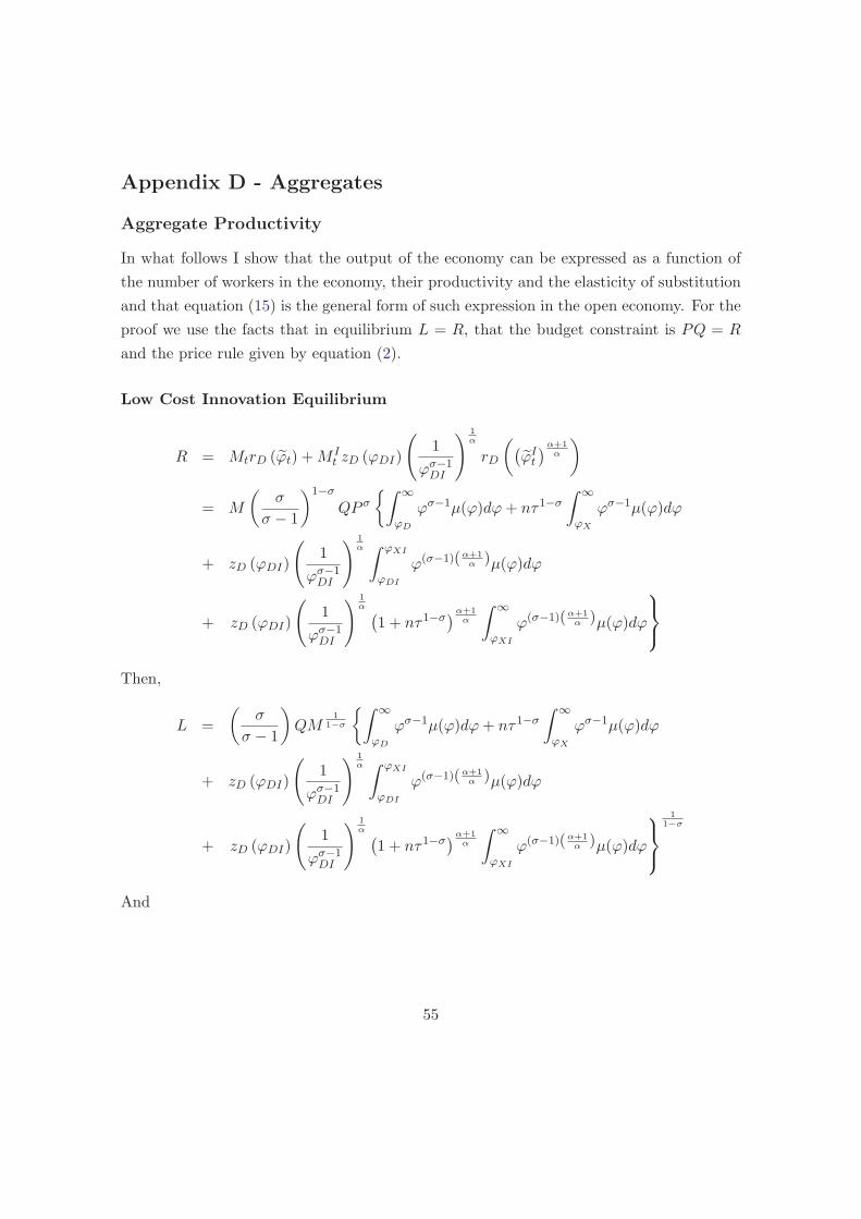
Appendix D - Aggregates

Aggregate Productivity

In what follows I show that the output of the economy can be expressed as a function of

the number of workers in the economy, their productivity and the elasticity of substitution

and that equation (15) is the general form of such expression in the open economy. For the

proof we use the facts that in equilibrium L = R, that the budget constraint is PQ = R

and the price rule given by equation (2).

Low Cost Innovation Equilibrium

R = MtrD (ϕt) +M It zD (ϕDI)

(1

ϕσ−1DI

) 1α

rD

((ϕIt

)α+1α

)

= M

(σ

σ − 1

)1−σ

QP σ

{∫ ∞

ϕD

ϕσ−1μ(ϕ)dϕ+ nτ1−σ

∫ ∞

ϕX

ϕσ−1μ(ϕ)dϕ

+ zD (ϕDI)

(1

ϕσ−1DI

) 1α ∫ ϕXI

ϕDI

ϕ(σ−1)(α+1α )μ(ϕ)dϕ

+ zD (ϕDI)

(1

ϕσ−1DI

) 1α (

1 + nτ1−σ)α+1

α

∫ ∞

ϕXI

ϕ(σ−1)(α+1α )μ(ϕ)dϕ

⎫⎬⎭Then,

L =

(σ

σ − 1

)QM

11−σ

{∫ ∞

ϕD

ϕσ−1μ(ϕ)dϕ+ nτ1−σ

∫ ∞

ϕX

ϕσ−1μ(ϕ)dϕ

+ zD (ϕDI)

(1

ϕσ−1DI

) 1α ∫ ϕXI

ϕDI

ϕ(σ−1)(α+1α )μ(ϕ)dϕ

+ zD (ϕDI)

(1

ϕσ−1DI

) 1α (

1 + nτ1−σ)α+1

α

∫ ∞

ϕXI

ϕ(σ−1)(α+1α )μ(ϕ)dϕ

⎫⎬⎭1

1−σ

And

55

Q =

(σ − 1

σ

)[M

(ΨD +

(1 + nτ1−σ

)ΨX + ILCI

(ΨDI +

(1 + nτ1−σ

)α+1α ΨXI

))] 1σ−1

L

(D.1)

where ILCI = zD (ϕDI)(

1ϕσ−1DI

) 1α, ΨD =

∫ ϕXI

ϕDϕ(σ−1)μ(ϕ)dϕ, ΨX =

∫∞ϕXI

ϕ(σ−1)μ(ϕ)dϕ,

ΨDI =∫ ϕXI

ϕDIϕ(σ−1)(α+1

α )μ(ϕ)dϕ and ΨXI =∫∞ϕXI

ϕ(σ−1)(α+1α )μ(ϕ)dϕ

Intermediate Equilibrium

R = MtrD (ϕt) +mXI

(1 + nτ1−σ

)zX (ϕXI)

(1

ϕσ−1XI

) 1α

rD

((ϕXI)

α+1α

)= M

(σ

σ − 1

)1−σ

QP σ

{∫ ∞

ϕD

ϕσ−1μ(ϕ)dϕ+ nτ1−σ

∫ ∞

ϕX

ϕσ−1μ(ϕ)dϕ

+ zX (ϕXI)

(1

ϕσ−1XI

) 1α (

1 + nτ1−σ) ∫ ∞

ϕXI

ϕ(σ−1)(α+1α )μ(ϕ)dϕ

⎫⎬⎭Then,

L =

(σ

σ − 1

)QM

11−σ

{∫ ∞

ϕD

ϕσ−1μ(ϕ)dϕ+ nτ1−σ

∫ ∞

ϕX

ϕσ−1μ(ϕ)dϕ

+ zX (ϕXI)

(1

ϕσ−1XI

) 1α (

1 + τ1−σ) ∫ ∞

ϕXI

ϕ(σ−1)(α+1α )μ(ϕ)dϕ

⎫⎬⎭1

1−σ

And

Q =

(σ − 1

σ

)[M(ΨD +

(1 + nτ (1−σ)

)ΨX + IIE

(1 + τ1−σ

)ΨXI

)] 1σ−1

L (D.2)

where IIE = zX (ϕXI)(

1ϕσ−1XI

) 1α, ΨD =

∫ ϕXI

ϕDϕ(σ−1)μ(ϕ)dϕ, ΨX =

∫∞ϕXI

ϕ(σ−1)μ(ϕ)dϕ and

ΨXI =∫∞ϕXI

ϕ(σ−1)(α+1α )μ(ϕ)dϕ

56

Low Cost Trade Equilibrium

R = MtrD (ϕt) +mXI

(1 + nτ1−σ

)zX(ϕXI)

(1

ϕσ−1XI

) 1α

rD

(ϕ(α+1

α )XI

)

= M

(σ

σ − 1

)1−σ

QP σ

{∫ ∞

ϕD

ϕσ−1μ(ϕ)dϕ+ nτ1−σ

∫ ∞

ϕX

ϕσ−1μ(ϕ)dϕ

+(1 + nτ1−σ

)zX(ϕXI)

(1

ϕσ−1XI

) 1α ∫ ∞

ϕXI

ϕ(σ−1)(α+1α )μ(ϕ)dϕ

⎫⎬⎭Then,

L =

(σ

σ − 1

)QM

11−σ

{∫ ∞

ϕD

ϕσ−1μ(ϕ)dϕ+ nτ1−σ

∫ ∞

ϕX

ϕσ−1μ(ϕ)dϕ

+(1 + nτ1−σ

)zX(ϕXI)

(1

ϕσ−1XI

) 1α ∫ ∞

ϕXI

ϕ(σ−1)(α+1α )μ(ϕ)dϕ

⎫⎬⎭1

1−σ

And

Q =

(σ − 1

σ

)[M(ΨD + (1 + nτ1−σ)ΨX + ILCT

(1 + nτ1−σ

)ΨXI

)] 1σ−1 L (D.3)

where ILCT = zX(ϕXI)(

1ϕσ−1XI

) 1α,ΨD =

∫ ϕX

ϕDϕ(σ−1)μ(ϕ)dϕ, ΨX =

∫∞ϕX

ϕ(σ−1)μ(ϕ)dϕ and

ΨXI =∫∞ϕXI

ϕ(σ−1)(α+1α )μ(ϕ)dϕ

Proof of Proposition 4

Low Cost Innovation Equilibrium

ΨLCI =

[M

(ΨD +

(1 + nτ1−σ

)ΨX + ILCI

(ΨDI +

(1 + nτ1−σ

)α+1α ΨXI

))] 1σ−1

57

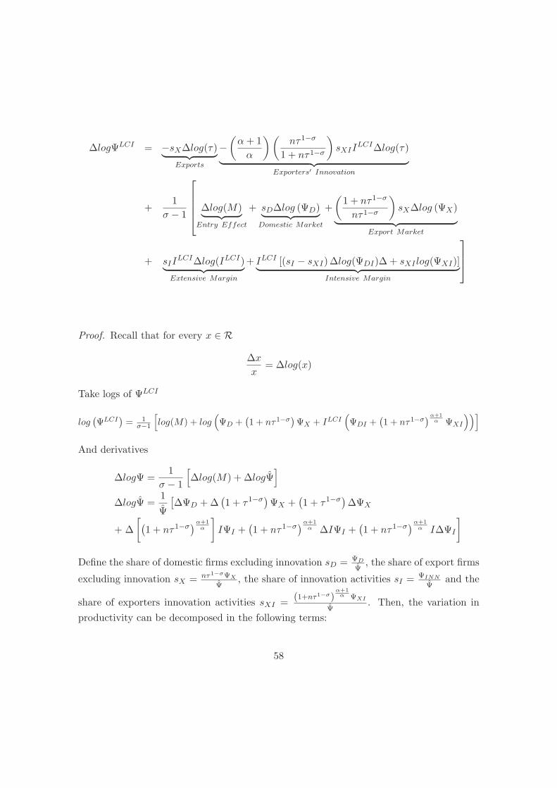
ΔlogΨLCI = −sXΔlog(τ)︸ ︷︷ ︸Exports

−(α+ 1

α

)(nτ1−σ

1 + nτ1−σ

)sXII

LCIΔlog(τ)︸ ︷︷ ︸Exporters′ Innovation

+1

σ − 1

⎡⎢⎢⎢⎣ Δlog(M)︸ ︷︷ ︸Entry Effect

+ sDΔlog (ΨD)︸ ︷︷ ︸Domestic Market

+

(1 + nτ1−σ

nτ1−σ

)sXΔlog (ΨX)︸ ︷︷ ︸

Export Market

+ sIILCIΔlog(ILCI)︸ ︷︷ ︸

Extensive Margin

+ ILCI [(sI − sXI)Δlog(ΨDI)Δ + sXI log(ΨXI)]︸ ︷︷ ︸Intensive Margin

⎤⎥⎦

Proof. Recall that for every x ∈ R

Δx

x= Δlog(x)

Take logs of ΨLCI

log(ΨLCI

)= 1

σ−1

[log(M) + log

(ΨD +

(1 + nτ1−σ

)ΨX + ILCI

(ΨDI +

(1 + nτ1−σ

)α+1α ΨXI

))]And derivatives

ΔlogΨ =1

σ − 1

[Δlog(M) + ΔlogΨ

]ΔlogΨ =

1

Ψ

[ΔΨD +Δ

(1 + τ1−σ

)ΨX +

(1 + τ1−σ

)ΔΨX

+ Δ

[(1 + nτ1−σ

)α+1α

]IΨI +

(1 + nτ1−σ

)α+1α ΔIΨI +

(1 + nτ1−σ

)α+1α IΔΨI

]Define the share of domestic firms excluding innovation sD = ΨD

Ψ, the share of export firms

excluding innovation sX = nτ1−σΨX

Ψ, the share of innovation activities sI = ΨINN

Ψand the

share of exporters innovation activities sXI =(1+nτ1−σ)

α+1α ΨXI

Ψ. Then, the variation in

productivity can be decomposed in the following terms:

58

� Direct Effect on Exports = −sXΔlog(τ)

� Direct Effect on Exporters’ Innovation = − (α+1α

) (nτ1−σ

1+nτ1−σ

)sXII

LCIΔlog(τ)

� Indirect Entry Effect =(

1σ−1

)Δlog(M)

� Indirect Domestic Market Effect =(

1σ−1

)sDΔlog (ΨD)

� Indirect Export Market Effect =(

1σ−1

)(1+nτ1−σ

nτ1−σ

)sXΔlog (ΨX)

� Indirect Extensive Margin Innovation Effect =(

1σ−1

)sII

LCIΔlog(ILCI)

� Indirect Intensive Margin Innovation Effect =(

1σ−1

)ILCI (sI − sXI)Δlog(ΨDI) +

(1

σ−1

)ILCIsXIΔlog

Intermediate Equilibrium

ΨIE =[M(ΨD +

(1 + nτ (1−σ)

)ΨX + IIE

(1 + nτ1−σ

)ΨXI

)] 1σ−1

ΔlogΨIE = −sXΔlog(τ)︸ ︷︷ ︸Exports

−(

nτ1−σ

1 + nτ1−σ

)sXII

IEΔlog(τ)︸ ︷︷ ︸Exporters′ Innovation

+1

σ − 1

⎡⎢⎢⎢⎣ Δlog(M)︸ ︷︷ ︸Entry Effect

+ sDΔlog (ΨD)︸ ︷︷ ︸Domestic Market

+

(1 + nτ1−σ

nτ1−σ

)sXΔlog (ΨX)︸ ︷︷ ︸

Export Market

+ sXIIIEΔlog(IIE)︸ ︷︷ ︸

Extensive Margin

+ IIEsXI log(ΨI)︸ ︷︷ ︸Intensive Margin

⎤⎥⎦

Proof. Recall that for every x ∈ R

Δx

x= Δlog(x)

59

Take logs of ΨIE

log(ΨIE

)=

1

σ − 1

[log(M) + log

(ΨD +

(1 + nτ1−σ

)ΨX + IIE

(1 + nτ1−σ

)ΨI

)]And derivatives

ΔlogΨ =1

σ − 1

[Δlog(M) + ΔlogΨ

]ΔlogΨ =

1

Ψ

[ΔΨD +Δ

(1 + nτ1−σ

)ΨX +

(1 + nτ1−σ

)ΔΨX

+ Δ(1 + nτ1−σ

)IΨI +

(1 + nτ1−σ

)ΔIΨI +

(1 + nτ1−σ

)IΔΨI

]Define the share of domestic firms excluding innovation sD = ΨD

Ψ, the share of export

firms excluding innovation sX = nτ1−σΨX

Ψand the share of exporters innovation activities

sXI =(1+nτ1−σ)ΨI

Ψ. Then, the variation in productivity can be decomposed in the following

terms:

� Direct Effect on Exports = −sXΔlog(τ)

� Direct Effect on Exporters’ Innovation = −(

nτ1−σ

1+nτ1−σ

)sXII

IEΔlog(τ)

� Indirect Entry Effect =(

1σ−1

)Δlog(M)

� Indirect Domestic Market Effect =(

1σ−1

)sDΔlog (ΨD)

� Indirect Export Market Effect =(

1σ−1

)(1+nτ1−σ

nτ1−σ

)sXΔlog (ΨX)

� Indirect Extensive Margin Innovation Effect =(

1σ−1

)sXII

IEΔlog(IIE)

� Indirect Intensive Margin Innovation Effect =(

1σ−1

)sXII

IEΔlog(ΨXI)

Low Cost Trade Equilibrium

ΨLCT =[M(ΨD + (1 + nτ1−σ)ΨX + ILCT

(1 + nτ1−σ

)ΨXI

)] 1σ−1

60

ΔlogΨLCT = −sXΔlog(τ)︸ ︷︷ ︸Exports

−sXIILCTΔlog(τ)︸ ︷︷ ︸

Exporters′ Innovation

+1

σ − 1

⎡⎢⎢⎢⎣ Δlog(M)︸ ︷︷ ︸Entry Effect

+ sDΔlog (ΨD)︸ ︷︷ ︸Domestic Market

+

(1 + nτ1−σ

nτ1−σ

)sXΔlog (ΨX)︸ ︷︷ ︸

Export Market

+

(1 + nτ1−σ

nτ1−σ

)sXII

LCTΔlog(ILCT )︸ ︷︷ ︸Extensive Margin

+

(1 + nτ1−σ

nτ1−σ

)sXII

LCT log(ΨI)︸ ︷︷ ︸Intensive Margin

⎤⎥⎥⎥⎦

Proof. Recall that for every x ∈ R

Δx

x= Δlog(x)

Take logs of ΨLCT

log(ΨLCT

)=

1

σ − 1

[log(M) + log

(ΨD +

(1 + nτ1−σ

)ΨX + ILCT

(1 + nτ1−σ

)ΨI

)]And derivatives

ΔlogΨ =1

σ − 1

[Δlog(M) + ΔlogΨ

]ΔlogΨ =

1

Ψ

[ΔΨD +Δ

(1 + nτ1−σ

)ΨX +

(1 + nτ1−σ

)ΔΨX

+ Δ(1 + nτ1−σ

)IΨI +

(1 + nτ1−σ

)ΔIΨI +

(1 + nτ1−σ

)IΔΨI

]Define the share of domestic firms excluding innovation sD = ΨD

Ψ, the share of export firms

excluding innovation sX = nτ1−σΨX

Ψand the share of exporters innovation activities sXI =

(1+nτ1−σ)ΨXI

Ψ. Then, the variation in productivity can be decomposed in the following

terms:

� Direct Effect on Exports = −sXΔlog(τ)

61

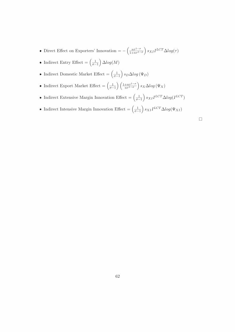
� Direct Effect on Exporters’ Innovation = −(

nτ1−σ

1+nτ1−σ

)sXII

LCTΔlog(τ)

� Indirect Entry Effect =(

1σ−1

)Δlog(M)

� Indirect Domestic Market Effect =(

1σ−1

)sDΔlog (ΨD)

� Indirect Export Market Effect =(

1σ−1

)(1+nτ1−σ

nτ1−σ

)sXΔlog (ΨX)

� Indirect Extensive Margin Innovation Effect =(

1σ−1

)sXII

LCTΔlog(ILCT )

� Indirect Intensive Margin Innovation Effect =(

1σ−1

)sXII

LCTΔlog(ΨXI)

62