APPROXIMATING THREE-DIMENSIONAL FLUID FLOW IN A MICROFLUIDIC DEVICE WITH A TWO-DIMENSIONAL, DEPTH-AVERAGED LATTICE BOLTZMANN METHOD

BY

ARTIN LALEIAN

THESIS

Submitted in partial fulfillment of the requirements for the degree of Master of Science in Environmental Engineering in Civil Engineering

in the Graduate College of the University of Illinois at Urbana-Champaign, 2014

Urbana, Illinois

Advisers:

Professor Albert J. Valocchi Professor Charles J. Werth

ii

ABSTRACT

Microfluidic devices (MFDs) are important tools in the study of reactive transport processes in

porous media. Laboratory and numerical experiments have studied reactions such as bimolecular

complexation, biodegradation and biofilm growth, and mineral precipitation coupled to fluid flow in

MFDs that are shallow rectangular channels with regular or irregular interior pore structure. The success

of these reactive transport models is dependent on accurate determination of the velocity field, because

reaction is coupled to solute transport. The small aspect ratio of these devices has led to their

approximation as two-dimensional (2D) objects in numerical models. This approximation may neglect

significant three-dimensional (3D) effects on the velocity field and contribute to model error. To avoid the

computational cost of a 3D numerical model, some 3D effects may be approximated in a 2D model. In

prior work in the literature, viscous drag from the top and bottom boundary surfaces omitted by the 2D

simulation has been approximated and applied as an external body force acting on the fluid for the case of

constant depth throughout the MFD. This work generalizes the approximation to cases of variable depth

to account for the possibility of precipitate or biofilm formation along those surfaces omitted by the 2D

simulation. The 2D lattice Boltzmann method (LBM) is reformulated to solve the depth-averaged Stokes

equations and the viscous drag body force approximation is applied. The 2D, depth-averaged LBM is

benchmarked by comparison to depth-averaged results of the 3D LBM in several test geometries.

Excellent agreement is observed between the results of the two methods in contracting-expanding channel

geometries. Agreement is not as favorable in more complex flows, such as flow around a cylinder or in a

MFD unit cell. In addition, a comparison of run times demonstrates the reduction in computational cost

with the 2D, depth-averaged LBM.

iii

ACKNOWLEDGEMENTS

I would like to thank my graduate advisors, Professor Charles J. Werth and Professor

Albert J. Valocchi, for their guidance in completing this work, as well as Dr. Haihu Liu for his

help in answering questions along the way. In addition, I owe thanks to my family for their

unrelenting support of my graduate studies. Part of this work was supported by the Department

of Energy Environmental Remediation Science Program, under award numbers DE-SC0001280

and DE-SC0006771. This material is based upon work supported by the National Science

Foundation Graduate Research Fellowship Program under Grant Number DGE-1144245.

iv

TABLE OF CONTENTS

CHAPTER 1: INTRODUCTION ................................................................................................... 1

CHAPTER 2: THEORETICAL BACKGROUND ........................................................................ 6

CHAPTER 3: METHODS ............................................................................................................ 18

CHAPTER 4: RESULTS .............................................................................................................. 24

CHAPTER 5: DISCUSSION ........................................................................................................ 53

BIBLIOGRAPHY ......................................................................................................................... 55

APPENDIX A: SUMMARY OF ANALYTICAL SOLUTIONS FOR OPEN, RECTANGULAR CHANNEL FLOWS ..................................................................................................................... 57

APPENDIX B: DERIVATION OF THE 2D ANALYTICAL VELOCITY PROFILE WITH VISCOUS DRAG ......................................................................................................................... 59

APPENDIX C: INTEGRATION OF THE 2D ANALYTICAL VELOCITY PROFILE WITH VISCOUS DRAG ......................................................................................................................... 61

1

CHAPTER 1: INTRODUCTION

Pore-scale reactive transport processes, such as bimolecular complexation and carbonate

mineral precipitation, have been studied with microfluidic devices (MFDs), model porous media

with simple interior pore structure composed of silicon (Willingham et al. 2008, Zhang et al.

2010). Carbonate precipitation is of interest in carbon capture and storage (CCS) systems

because precipitate buildup can reduce aquifer storage capacity by blocking pores, thereby

reducing the aquifer's effective porosity. Understanding the dynamics of subsurface mineral

precipitation is vital to predicting the success of CCS systems. MFD experiments have also been

used to study other important processes such as biodegradation with biofilm growth (Nambi et al.

2003), and multiphase flow. Laboratory and numerical experiments with MFDs aim to

characterize the complex dynamics involved in subsurface transport and reaction.

The exterior geometry of a MFD is a shallow rectangular channel, with a cross-sectional

depth to width ratio on the order of 10−3, as depicted in Figure 1. Because the flow depth is small

relative to the flow width, numerical models have approximated the MFD as a two-dimensional

(2D) system by neglecting its depth and employing 2D numerical methods for solute transport

and reaction (Willingham et al. 2008, Willingham et al. 2010). The primary motivator for

reducing the MFD’s physical dimensions is the accompanying reduction in computational cost of

Figure 1: Top and side views of MFD. Lengths are not to scale. Actual MFD contains many more cylindrical pillars than depicted here.

2

the numerical model.

Still, the three-dimensional (3D) nature of the system cannot be completely ignored. The

2D model of Yoon et al. (2012) implicitly includes the MFD’s depth by confining precipitate

growth to the top and bottom surfaces of the MFD, which are not explicitly present in the 2D

domain. In Figure 3, the centered horizontal line is the plane included in the simulation and the

solid blocks are mineral precipitate, assumed to grow symmetrically above and below that plane.

Their model tracks precipitate accumulation outside the plane, assuming complete blockage to

flow when this amount exceeds a threshold value. Thus, the MFD’s interior depth is both

transient and spatially-variable as precipitate can grow and dissolve from the implicit top and

bottom surfaces.

Neglecting a spatial dimension of the MFD results in model error due to 3D effects not

captured in the 2D approximation. For example, the top and bottom surfaces impart viscous drag

that reduces fluid speed, and local variation in depth redirects flow, e.g. away from highly-

Figure 3: Magnified side view of MFD. The centered horizontal line represents the domain of the 2D simulation. Symmetric precipitate growth is shown from the top and bottom surfaces.

Figure 2: Scanning electron microscope image of cylindrical pillars in real MFD.

3

blocked regions. Existing 2D models do not capture these effects. We propose an improved

approach to determine a 2D velocity field in the MFD with a depth-averaged lattice Boltzmann

method (LBM) that incorporates the 3D effects of viscous drag with depth variation.

To define a successful 2D representation of the depth-averaged true 3D velocity field,

first assume a 3D velocity field is available, denoted 𝒖𝟑𝟑(𝑥,𝑦, 𝑧) = �𝑢3𝐷,𝑥 𝑢3𝐷,𝑦 𝑢3𝐷,𝑧�𝑇. It is a

function of three spatial coordinates and may be obtained by the 3D LBM or other fluid flow

solver. Its 2D representation is obtained by averaging across the MFD’s depth, yielding three

depth-averaged velocity components. After omitting the vertical component, the resulting 2D

velocity field may be denoted 𝒖�𝟑𝟑(𝑥, 𝑦) = �𝑢�3𝐷,𝑥 𝑢�3𝐷,𝑦 �𝑇. For the purposes of this

work, 𝒖�𝟑𝟑(𝑥, 𝑦) is the desired solution for flow in the MFD. The middle column in the diagram

below summarizes the process just described.

Our goal is to obtain 𝒖�𝟑𝟑 while avoiding the computational cost of determining the 3D

velocity field. The model of Yoon et al. (2012) determines the 2D velocity field by solving the

2D Stokes equations with the LBM (left column of the diagram). However, the resulting 2D

Flow diagram describing various approaches to solution

Existing

Approach True Solution

Proposed

Approach

2D Stokes Eqs.

3D Stokes Eqs.

3D Stokes Eqs.

solve

numerically

solve

numerically

depth-

average

3D vel. field (𝒖𝟑𝟑)

2D D-A Stokes Eqs.

depth-

average

solve

numerically

2D vel. field ≠ 2D vel. field (𝒖�𝟑𝟑) ? 2D vel. field (𝒖𝟐𝟑)

4

velocity field may not closely approximate 𝒖�𝟑𝟑 in local velocity. As a simple example,

transverse analytical velocity profiles are compared in Figure 4 for flow in an open, constant-

depth 2D channel. Analytical velocity profiles, which will be discussed in more detail, are

available in Appendix A. One velocity profile includes the 3D effect of viscous drag from the

implicit top and bottom surfaces. The other profile does not include this effect, resulting in the

characteristic parabolic profile of Poiseulle flow. Under identical pressure gradient and fluid

viscosity, the two analytical profiles match neither in total flow rate nor in shape. The flow rate

may be matched by scaling one velocity profile, but there could still be some error in local

velocity.

An alternative approach is summarized in the right column of the diagram. First, the 3D

Stokes equations are depth-averaged, yielding three equations in three depth-averaged velocity

components. The equation in the vertical component is omitted, leaving two governing equations

to be solved numerically. The 2D LBM can be modified to solve these depth-averaged equations.

Ideally, the resulting 2D velocity field, denoted 𝒖𝟐𝟑(𝑥, 𝑦) = �𝑢2𝐷,𝑥 𝑢2𝐷,𝑦�𝑇, closely

approximates 𝒖�𝟑𝟑. If so, we have obtained an improved 2D velocity field without first

Figure 4: Transverse velocity profile in an open, constant-depth 2D channel, with and without viscous drag from implicit top and bottom

surfaces. Without viscous drag is Poiseuille flow.

5

determining a 3D velocity field.

The reduction in computational cost relative to a 3D approach is not the only benefit of

the proposed 2D approach. Note that in both a 2D and 3D model, precipitate may grow in such a

way as to produce narrow constrictions to flow that are spanned by only a few fluid nodes. With

fewer than four fluid nodes within such a constriction, the LBM is not expected to produce a

realistic velocity field (Succi 2001). Thus, there is a limit on how narrow a constriction should be

allowed in the model to maintain model accuracy. In a 3D model, without confining precipitate

growth to any surfaces, a narrow constriction would be problematic across the width or depth of

the MFD. In a 2D model with implicit depth, only narrow constrictions across the width would

be problematic.

Second, note that precipitate growth and dissolution is represented in a 3D model by

changing the state of a node between solid and fluid. Thus, precipitation and dissolution only

occur in discrete quantities, namely integer multiples of the node spacing, Δ𝑥. With the 2D

approach the implicit MFD depth can take any real value greater than zero, meaning

precipitation and dissolution can occur continuously. This is an improvement over the 3D

method, because precipitate growth and dissolution are not constrained by the lattice in the

vertical direction. Still, the horizontal position of precipitate is confined to nodes in the 2D

domain.

6

CHAPTER 2: THEORETICAL BACKGROUND

2.1 The Lattice Boltzmann Method (LBM)

2.1.1 Choice of Lattice

The LBM is a mesoscopic numerical method for fluid simulation on a regular lattice in

one, two, or three spatial dimensions. Each lattice node is connected to a subset (possibly all)

neighboring nodes via lattice vectors, denoted 𝒆𝒊. In the following text, vector symbols will

appear in bold font and scalars in plain font. The set of lattice vectors defines all possible fluid

particle velocities, requiring that particles remain on the lattice. When implementing the LBM,

the choice of lattice and its connectivity depend on the spatial dimensions of the problem at hand

and the available computational resources. Common lattice nomenclature takes the following

form. .

D (number of spatial dimensions) Q (lattice connectivity)

In the above expression, the number of spatial dimensions is most often two or three and

the lattice connectivity is the size of the set of lattice vectors. D2Q9 and D3Q15 lattices are often

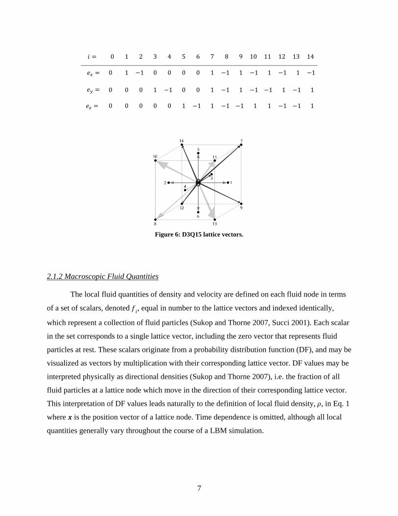
encountered in the literature, and will be implemented in this work. Lattice vectors, 𝒆𝒊, for the

D2Q9 and D3Q15 lattices, indexed 𝑖 = 0, 1, . . . , 8 and 𝑖 = 0, 1, . . . , 14, respectively, are defined

below for a unit lattice, with visual depictions in Figure 5 and Figure 6.

𝑖 = 0 1 2 3 4 5 6 7 8

𝑒𝑥 = 0 1 0 −1 0 1 −1 −1 1

𝑒𝑦 = 0 0 1 0 −1 1 1 −1 −1

Figure 5: D2Q9 lattice vectors.

7

2.1.2 Macroscopic Fluid Quantities

The local fluid quantities of density and velocity are defined on each fluid node in terms

of a set of scalars, denoted 𝑓𝑖, equal in number to the lattice vectors and indexed identically,

which represent a collection of fluid particles (Sukop and Thorne 2007, Succi 2001). Each scalar

in the set corresponds to a single lattice vector, including the zero vector that represents fluid

particles at rest. These scalars originate from a probability distribution function (DF), and may be

visualized as vectors by multiplication with their corresponding lattice vector. DF values may be

interpreted physically as directional densities (Sukop and Thorne 2007), i.e. the fraction of all

fluid particles at a lattice node which move in the direction of their corresponding lattice vector.

This interpretation of DF values leads naturally to the definition of local fluid density, 𝜌, in Eq. 1

where 𝒙 is the position vector of a lattice node. Time dependence is omitted, although all local

quantities generally vary throughout the course of a LBM simulation.

𝑖 = 0 1 2 3 4 5 6 7 8 9 10 11 12 13 14

𝑒𝑥 = 0 1 −1 0 0 0 0 1 −1 1 −1 1 −1 1 −1

𝑒𝑦 = 0 0 0 1 −1 0 0 1 −1 1 −1 −1 1 −1 1

𝑒𝑧 = 0 0 0 0 0 1 −1 1 −1 −1 1 1 −1 −1 1

Figure 6: D3Q15 lattice vectors.

8

𝜌(𝒙) = �𝑓𝑖(𝒙)

𝑖

Eq. 1

Local fluid momentum is a weighted sum of lattice vectors, the weights being DF values.

Extending the previous physical interpretation, terms in the summation below may be considered

directional momenta, their sum yielding the local net momentum.

𝜌𝒖 = �𝑓𝑖𝒆𝒊𝑖

Eq. 2

Pressure and density are related by the equation of state for an ideal gas, where 𝑐𝑠 is the

speed of sound on the lattice, a constant for all lattices implemented in this work.

𝑑 = 𝜌𝑐𝑠2 𝑐𝑠 =1√3

Fluid kinematic viscosity is a function of a parameter 𝜏, related to the interaction of fluid

particles, as described shortly. In the equation below, Δ𝑡 is the lattice time step, most often given

a value of one (Sukop and Thorne 2007).

𝜈 = 𝑐𝑠2 �𝜏 −

Δ𝑡2� Eq. 3

2.1.3 The Lattice Boltzmann Algorithm

The LBM proceeds in two sequential fundamental steps named streaming and collision.

Each step may be understood from its purpose in lattice gas cellular automata (LGCA) models, a

predecessor of the LBM that simulates a fluid with single particles on a regular lattice. In LGCA,

streaming consists of propagating single particles one lattice node in their given direction of

travel, or simply free motion of particles. Collision, as the name implies, involves accounting for

interparticle collisions at each lattice node in such a way as to conserve local mass and

momentum. The earliest LGCA models allowed only head-on collisions between two particles,

which reversed their direction of travel, while later models considered additional possibilities.

Streaming and collision are stated mathematically by the first and second equations below,

respectively. The right-hand side (RHS) of the second equation is written in operator notation,

9

where Ω denotes the collision operator.

Streaming: 𝑓𝑖(𝒙 + 𝒆𝒊Δ𝑡, 𝑡 + Δ𝑡) = 𝑓𝑖(𝒙, 𝑡 + Δ𝑡)

Collision: 𝑓𝑖(𝒙, 𝑡 + Δ𝑡) = Ω[𝑓𝑖(𝒙, 𝑡)]

In the LBM, streaming consists of free motion of DF values, in which they are

propagated by one lattice node in the direction of their respective lattice vector. The LBM does

not stream single particles, but a collection of particles represented by a DF value. As in the

LGCA, collision in the LBM consists of accounting for local interparticle interactions. It is not

immediately clear how to account for collision with DF values as opposed to single particles. As

with LGCA, mass and momentum should be conserved in the LBM collision. The most common

solution to this problem represents collision as a relaxation of DF values toward a local

equilibrium, known as the BGK operator after its original authors (Bhatnagar et al. 1954). Local

equilibrium is defined as a second-order Taylor expansion of the Maxwell distribution, shown in

Eq. 4. Although not explicitly shown, both 𝜌 and 𝒖 are local quantities, 𝜌 = 𝜌(𝒙) and 𝒖 = 𝒖(𝒙).

𝑤𝑖 are directional weights, which may be interpreted as variable particle masses across different

lattice directions (Succi 2001). Values of 𝑤𝑖 for the D2Q9 and D3Q15 lattices are shown below.

𝑓𝑖𝑎𝑒(𝜌,𝒖) = 𝑤𝑖𝜌 �1 + 3(𝒆𝒊 ⋅ 𝒖) +

92

(𝒆𝒊 ⋅ 𝒖)2 −32

(𝒖 ⋅ 𝒖)� Eq. 4

D2Q9 D3Q15

𝑤𝑖 = �

4/9 𝑖 = 01/9 𝑖 = 1 − 4

1/36 𝑖 = 5 − 8 𝑤𝑖 = �

2/9 𝑖 = 01/9 𝑖 = 1 − 6

1/72 𝑖 = 7 − 14

Relaxation toward local equilibrium means that during collision, 𝑓𝑖 are shifted toward 𝑓𝑖𝑎𝑒

at a rate given by the relaxation parameter, 𝜏. The BGK collision operator is expressed explicitly

below.

Ω[𝑓𝑖(𝒙, 𝑡)] = 𝑓𝑖(𝒙, 𝑡) −𝑓𝑖(𝒙, 𝑡) − 𝑓𝑖

𝑎𝑒(𝜌,𝒖)𝜏

The streaming and collision equations are now combined, with the BGK collision

10

operator included.

𝑓𝑖(𝒙 + 𝒆𝒊Δ𝑡, 𝑡 + Δ𝑡) = 𝑓𝑖(𝒙, 𝑡) −

𝑓𝑖(𝒙, 𝑡) − 𝑓𝑖𝑎𝑒(𝜌,𝒖)

𝜏 Eq. 5

2.2 The Incompressible Lattice Boltzmann Formulation

The LBM implementation described above (hereby referred to as the standard LBM)

recovers the compressible Navier-Stokes (N-S) equations to second-order accuracy. Many

applications aim to simulate incompressible flow, however, and an alternative formulation of the

LBM is available (He and Luo 1997) which significantly reduces compressibility error. Under

the new formulation, the same process which recovered the compressible N-S equations to

second-order accuracy now recovers the incompressible N-S equations. Under the

incompressible formulation, local density is calculated as in Eq. 1. Velocity, however, is

calculated as momentum was in Eq. 2.

𝒖 = �𝑓𝑖𝒆𝒊

𝑖

Eq. 6

The equilibrium distribution function also differs from Eq. 4, and is expressed in Eq. 7.

As before, 𝜌 = 𝜌(𝒙) and 𝒖 = 𝒖(𝒙).

𝑓𝑖𝑎𝑒(𝜌,𝒖) = 𝑤𝑖 �𝜌 + 3(𝒆𝒊 ⋅ 𝒖) +

92

(𝒆𝒊 ⋅ 𝒖)2 −32

(𝒖 ⋅ 𝒖)� Eq. 7

2.3 Representation of Viscous Drag from Top and Bottom Surfaces

To characterize the viscous drag caused by the top and bottom surfaces of the MFD, first

consider flow in a 3D constant-depth rectangular channel. This is the outer shell of a MFD, with

no interior pore structure. Because the top and bottom surfaces are outside the 2D domain (refer

to Figure 3), the viscous drag they impart on the fluid has to be accounted for artificially. The

11

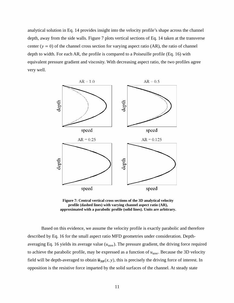
analytical solution in Eq. 14 provides insight into the velocity profile’s shape across the channel

depth, away from the side walls. Figure 7 plots vertical sections of Eq. 14 taken at the transverse

center (𝑦 = 0) of the channel cross section for varying aspect ratio (AR), the ratio of channel

depth to width. For each AR, the profile is compared to a Poiseuille profile (Eq. 16) with

equivalent pressure gradient and viscosity. With decreasing aspect ratio, the two profiles agree

very well.

Based on this evidence, we assume the velocity profile is exactly parabolic and therefore

described by Eq. 16 for the small aspect ratio MFD geometries under consideration. Depth-

averaging Eq. 16 yields its average value (𝑢𝑎𝑎𝑎). The pressure gradient, the driving force required

to achieve the parabolic profile, may be expressed as a function of 𝑢𝑎𝑎𝑎. Because the 3D velocity

field will be depth-averaged to obtain 𝒖�𝟑𝟑(𝑥,𝑦), this is precisely the driving force of interest. In

opposition is the resistive force imparted by the solid surfaces of the channel. At steady state

Figure 7: Central vertical cross sections of the 3D analytical velocity profile (dashed lines) with varying channel aspect ratio (AR),

approximated with a parabolic profile (solid lines). Units are arbitrary.

12

these forces are balanced, meaning the resistive viscous drag is equal in magnitude and opposite

in direction of the driving pressure gradient. Any contribution of drag from the side walls is

neglected. Replacing 𝑢𝑎𝑎𝑎 with the 2D LBM velocity, 𝒖𝟐𝟑, and dividing by 𝜌 provides an

expression for the acceleration due to viscous drag from the top and bottom surfaces.

An expression similar to 𝒂𝒅𝒅𝒂𝒅 (using the maximum rather than average of the Poiseuille

profile) was derived by Flekkoy et al. (1995) for the purpose of representing viscous drag in a

Hele-Shaw cell, and applied to a constant-depth MFD by Venturoli and Boek (2006). Eq. 8 has

been used by Boek and Venturoli (2010), also in a constant-depth channel.

2.4 Body Force Implementation

An external force may be included in the 2D LBM with an additional term in the collision

step, with the form of 𝐹𝑖 varying by implementation.

𝑓𝑖(𝒙 + 𝒆𝒊Δ𝑡, 𝑡 + Δ𝑡) = 𝑓𝑖(𝒙, 𝑡) −𝑓𝑖(𝒙, 𝑡) − 𝑓𝑖

𝑎𝑒(𝜌,𝒖)𝜏

+ 𝐹𝑖Δ𝑡

In addition, some implementations shift the velocity field (Guo et al. 2002). Although

some implementations have theoretical advantages over others, in practice there is little

𝑢𝑎𝑎𝑎 = �−

𝑑𝑑𝑑𝑥�ℎ2

12𝜇

𝑑𝑑𝑑𝑥

= −12𝜇ℎ2

𝑢𝑎𝑎𝑎

𝜌𝑎𝑥 = −

12𝜇ℎ2

𝑢𝑎𝑎𝑎

𝑎𝑥 = −

12𝜈ℎ2

𝑢𝑎𝑎𝑎

𝒂𝒅𝒅𝒂𝒅 = −

12𝜈ℎ2

𝒖𝟐𝟑 Eq. 8

13

difference between the numerical results obtained across implementations (Mohamad and

Kuzmin 2010). For this reason, we utilize the relatively simple implementation of Luo (2000),

where 𝐹𝑖 takes the general form in Eq. 9, with 𝒂 being the acceleration due to external forcing.

𝐹𝑖 = −3𝑤𝑖𝜌(𝒆𝒊 ⋅ 𝒂) Eq. 9

2.5 Depth-Averaged Lattice Boltzmann Formulation

For incompressible Stokes flow, the governing continuum equations are the continuity

and Stokes equations, where 𝒖 = 𝒖(𝑥, 𝑦, 𝑧).

∇𝒖 = 0

𝜇∇2𝒖 − ∇𝑑 = 0

The standard 2D LBM will solve the 2D counterparts of the above equations. We first

present an incomplete derivation of the depth-averaged continuum equations, then discuss the

modifications needed for the 2D LBM to solve these equations. Let 𝒖(𝑥,𝑦, 𝑧) = �𝑢𝑥 𝑢𝑦 𝑢𝑧�𝑇

and ℎ = ℎ(𝑥, 𝑦), the spatially-variable depth . The derivation below considers only the continuity

equation, but may be applied to the momentum equation as well. First, the equation is depth-

averaged.

1ℎ��

𝜕𝑢𝑥𝜕𝑥

ℎ

0𝑑𝑧 + �

𝜕𝑢𝑦𝜕𝑦

ℎ

0𝑑𝑧 + �

𝜕𝑢𝑧𝜕𝑧

ℎ

0𝑑𝑧� = 0

Multiply by h, evaluate the last term, and reverse operator order for the first two terms:

𝜕𝜕𝑥

� 𝑢𝑥ℎ

0𝑑𝑧 +

𝜕𝜕𝑦

� 𝑢𝑦ℎ

0𝑑𝑧 + 𝑢𝑧(𝑥,𝑦, ℎ) − 𝑢𝑧(𝑥,𝑦, 0) = 0

With solid surfaces at 𝑧 = 0 and 𝑧 = ℎ, i.e. the top and bottom walls, the vertical

component of flow must be 0, leaving:

𝜕𝜕𝑥

� 𝑢𝑥ℎ

0𝑑𝑧 +

𝜕𝜕𝑦

� 𝑢𝑦ℎ

0𝑑𝑧 = 0

14

The integrals describe component flow rates across the depth, which are equivalent to the

depth-averaged velocity component multiplied by depth.

𝜕(�̄�𝑥ℎ)𝜕𝑥

+𝜕(�̄�𝑦ℎ)𝜕𝑦

= 0

∇(𝒖�ℎ) = 0

𝒖� = ��̄�𝑥 �̄�𝑦�𝑇

Similarly, the Stokes equations, with drag term now included, transform as below.

∇(�̄�ℎ) = 𝜇∇2(�̄�ℎ) −12𝜇ℎ2

(�̄�ℎ)

Note that if ℎ is constant, the depth-averaged equations reduce to the standard 2D

continuum equations plus the viscous drag term. The depth-averaged equations differ from the

standard 2D governing equations with viscous drag term only by the substitution 𝒖 → �̄�ℎ. The

same substitution is used to reformulate the incompressible 2D LBM so that it solves the depth-

averaged governing equations. Local macroscopic velocity (Eq. 6) and the equilibrium

distribution function (Eq. 7) of the incompressible 2D LBM are redefined in Eq. 10 and Eq. 11.

𝒖(𝑥,𝑦) =

1ℎ(𝑥,𝑦)

�𝑓𝑖𝒆𝒊𝑖

Eq. 10

𝑓𝑖𝑎𝑒(𝜌,𝒖, ℎ) = 𝑤𝑖 �𝜌 + 3h(𝒆𝒊 ⋅ 𝒖) +

9h2

2(𝒆𝒊 ⋅ 𝒖)2 −

3h2

2(𝒖 ⋅ 𝒖)� Eq. 11

2.6 Boundary Conditions

2.6.1 Periodic

Periodic boundaries connect two ends of the computational lattice by treating their nodes

as adjacent to one another. The implementation requires no special treatment beyond the

streaming process, which should propagate DF values between opposite boundaries.

15

2.6.2 No-slip

A great strength of the LBM for applications in porous media is its straightforward

handling of complex solid-fluid boundaries. Each lattice node may be labeled as either solid or

fluid and a localized boundary condition implemented to satisfy the no-slip condition. In this

way the LBM can theoretically handle solid-fluid boundaries of arbitrary complexity. The most

simple no-slip implementation is the halfway bounceback boundary condition. Any DF value

which streams on to a solid node is reflected about the solid node so that it returns to its

originating fluid node in the next iteration of streaming (Sukop and Thorne 2007). The halfway

bounceback boundary effectively places the solid wall halfway between adjacent solid and fluid

nodes, a fact that should be accounted for when representing physical lengths with the lattice.

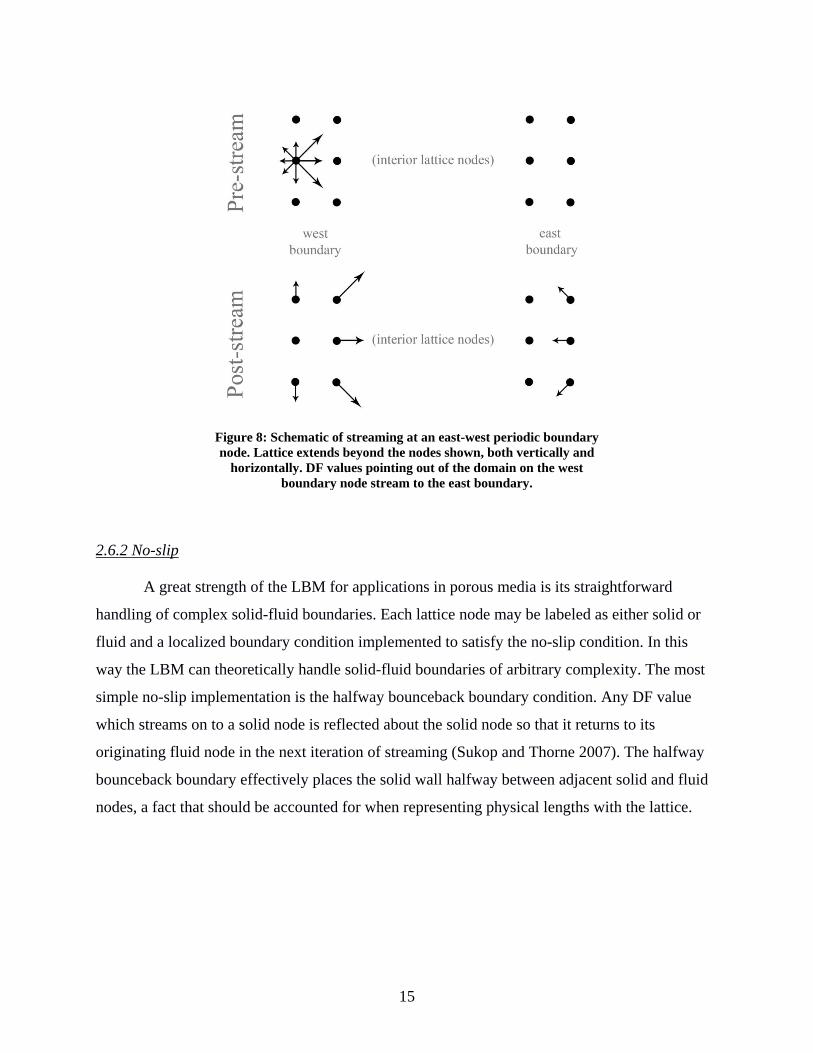
Figure 8: Schematic of streaming at an east-west periodic boundary node. Lattice extends beyond the nodes shown, both vertically and

horizontally. DF values pointing out of the domain on the west boundary node stream to the east boundary.

16

2.7 Unit Conversion

Most lattice Boltzmann implementations assign a value of one to both the node step Δ𝑥

and time step Δ𝑡 in lattice units. The former was implied by the lattice vectors 𝒆𝒊 defined earlier.

Δ𝑥𝑙 = 1 𝑛𝑜𝑑𝑒 𝑠𝑡𝑒𝑝

Δ𝑡𝑙 = 1 𝑡𝑖𝑚𝑒 𝑠𝑡𝑒𝑝

Subscripts of 𝑙 and 𝑝 will denote lattice and physical units, respectively. Conversion

between the two systems of units is possible, and will be used to refine the lattice in physical

units while maintaining the values of Δ𝑥𝑙 and Δ𝑡𝑙 above. The general approach will be to define a

physical system, convert it to a lattice system, determine a velocity field in lattice units, then

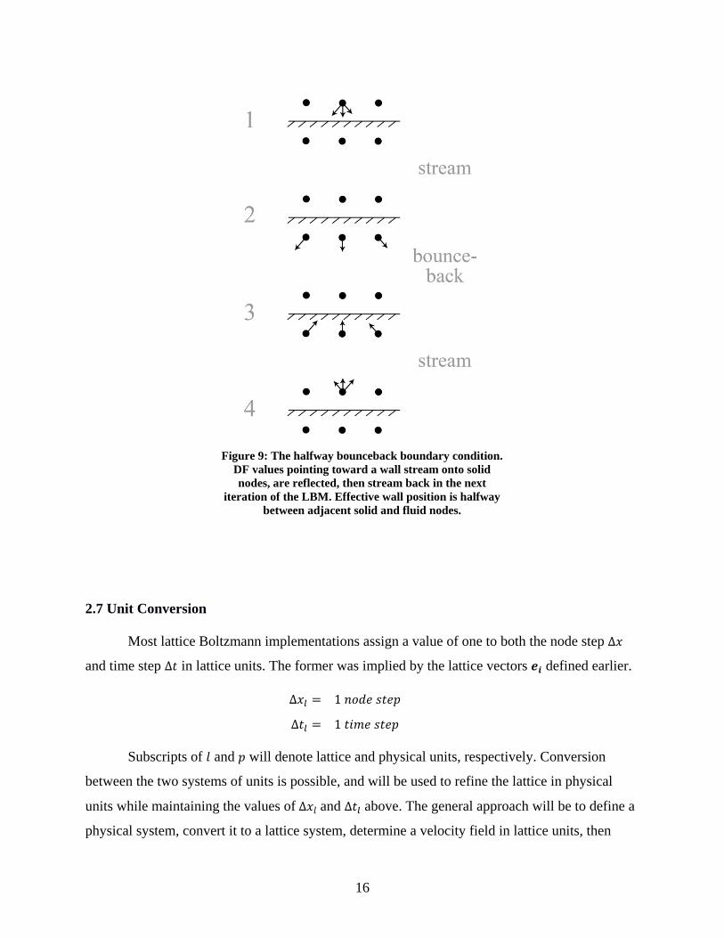
Figure 9: The halfway bounceback boundary condition. DF values pointing toward a wall stream onto solid nodes, are reflected, then stream back in the next

iteration of the LBM. Effective wall position is halfway between adjacent solid and fluid nodes.

17

convert it to a velocity field in physical units. Suppose conversion factors for length and time

have been specified in centimeters and seconds.

Δ𝑥𝑝 𝑐𝑚

𝑛𝑜𝑑𝑒 𝑠𝑡𝑒𝑝

Δ𝑡𝑝 𝑠𝑒𝑐

𝑡𝑖𝑚𝑒 𝑠𝑡𝑒𝑝

Any quantity involving length and time may be converted from a physical value to a

lattice value. Conversion of velocity and kinematic viscosity are shown below, with units

included in brackets.

𝑢𝑙 = 𝑢𝑝 �

𝑐𝑚𝑠𝑒𝑐

� ×1Δ𝑥𝑝

�𝑛𝑜𝑑𝑒 𝑠𝑡𝑒𝑝

𝑐𝑚� × Δ𝑡𝑝 �

𝑠𝑒𝑐𝑡𝑖𝑚𝑒 𝑠𝑡𝑒𝑝

�

𝑢𝑙 = 𝑢𝑝

Δ𝑡𝑝Δ𝑥𝑝

𝜈𝑙 = 𝜈𝑝 �

𝑐𝑚2

𝑠𝑒𝑐� ×

1Δ𝑥𝑝2

�𝑛𝑜𝑑𝑒 𝑠𝑡𝑒𝑝

𝑐𝑚�2

× Δ𝑡𝑝 �𝑠𝑒𝑐

𝑡𝑖𝑚𝑒 𝑠𝑡𝑒𝑝�

𝜈𝑙 = 𝜈𝑝

Δ𝑡𝑝Δ𝑥𝑝2

In principle, both Δ𝑥 and Δ𝑡 may be chosen freely. Δ𝑥 is selected to result in adequate

resolution of the physical system. A good rule of thumb for selecting Δ𝑡 is to scale it with Δ𝑥 by

the relation Δ𝑡 ~ Δ𝑥2, which derives from the requirement that compressibility error and

discretization error are the same order of magnitude (Latt 2008). We use the relation

Δ𝑡 = 5Δ𝑥2.

18

CHAPTER 3: METHODS

3.1 Lattice Boltzmann Code

The LBM in 2D and 3D is implemented in a custom Fortran code. In both 2D and 3D, the

code implements the incompressible formulation with an external body force. In the 2D method,

the body force consists of both a driving acceleration (i.e. pressure gradient) and a resistive

acceleration (i.e. viscous drag). In the 3D method, the body force consists of only a driving

acceleration. For standard LBM subroutines, see Sukop and Thorne (2007).

3.2 Depth-averaging the 3D Velocity Field

Although three components of the 3D velocity field 𝒖𝟑𝟑(𝑥,𝑦, 𝑧) may be depth-averaged,

only the streamwise (𝑢3𝐷,𝑥) and transverse (𝑢3𝐷,𝑦) components, i.e. those components parallel to

the horizontal plane, can be compared against 𝒖𝟐𝟑(𝑥,𝑦). Thus, the vertical component of the

depth-averaged 3D velocity field is omitted in 𝒖�𝟑𝟑(𝑥,𝑦).

𝒖�𝟑𝟑(𝑥,𝑦) =1

ℎ(𝑥,𝑦)� 𝒖𝟑𝟑(𝑥, 𝑦, 𝑧)ℎ(𝑥,𝑦)

0 𝑑𝑧

Numerical integration is performed using the composite trapezoidal approximation,

shown below for a series of 𝑛 + 1 equally-spaced points. The 𝑥 and 𝑦 coordinates are indexed

because integration is performed independently at each node in the horizontal plane. 𝑢 in the

equation below refers to a single component of velocity.

�𝑢(𝑥𝑖 ,𝑦𝑖 , 𝑧) 𝑑𝑧𝑏

𝑎

≈ �ℎ(𝑥𝑖 ,𝑦𝑖)

2𝑛� [𝑢(𝑥𝑖 ,𝑦𝑖 , 𝑧1) + 2𝑢(𝑥𝑖 ,𝑦𝑖 , 𝑧2) + ⋯+ 2𝑢(𝑥𝑖 ,𝑦𝑖 , 𝑧𝑛) + 𝑢(𝑥𝑖 ,𝑦𝑖 , 𝑧𝑛+1)]

19

3.3 Velocity Field Convergence

The LBM is iterated to steady-state, at which time simulated velocities fields are

compared. The velocity field is considered steady when the inequality below (Zou and He 1997)

is satisfied. Summations are evaluated over the entire lattice. The superscript * denotes the

velocity field may be either 𝒖𝟑𝟑(𝑥,𝑦, 𝑧) or 𝒖𝟐𝟑(𝑥,𝑦).

��‖𝒖∗(𝑡) − 𝒖∗(𝑡 − 1)‖2

∑‖𝒖∗(𝑡)‖𝟐< 10−6

3.4 Geometric Parameters

The entire MFD is not simulated due to computational limitations. Rather, the dimensions

of a representative unit cell are used to define the numerical lattice size. In the numerical

experiments to follow, the interior geometry will often differ from that shown in Figure 10, but

the exterior dimensions will not. The length, width, and depth of the 3D unit cell are 335, 335,

and 20 𝜇𝑚, respectively. These physical lengths are denoted 𝑙,𝑤, and ℎ. Note the 2D domain for

simulation has explicit dimensions of 𝑙,𝑤 and an implicit dimension ℎ, which may be spatially-

variable. Lattice node spacing should be selected to adequately resolve the cell’s depth, with no

less than four fluid nodes spanning the channel depth in order to produce realistic results (Succi

2001). Recall this is a consideration for the 3D simulation, where the cell’s depth is explicitly

defined. After defining the node spacing, the lattice dimensions, i.e. the number of nodes in each

dimension, are calculated as follows.

𝑛𝑥 =𝑙Δ𝑥

+ 1 𝑛𝑦 =𝑤Δ𝑥

+ 1 𝑛𝑧 =ℎΔ𝑥

+ 1

The expressions above should be modified by adding a value of one if halfway

bounceback boundaries are implemented, because they effectively place the solid wall halfway

between adjacent fluid and solid nodes. The loss of length Δ𝑥/2 near each wall is balanced by

addition of an extra node, thereby adding a length of Δ𝑥 to the dimension containing two halfway

bounceback boundaries.

20

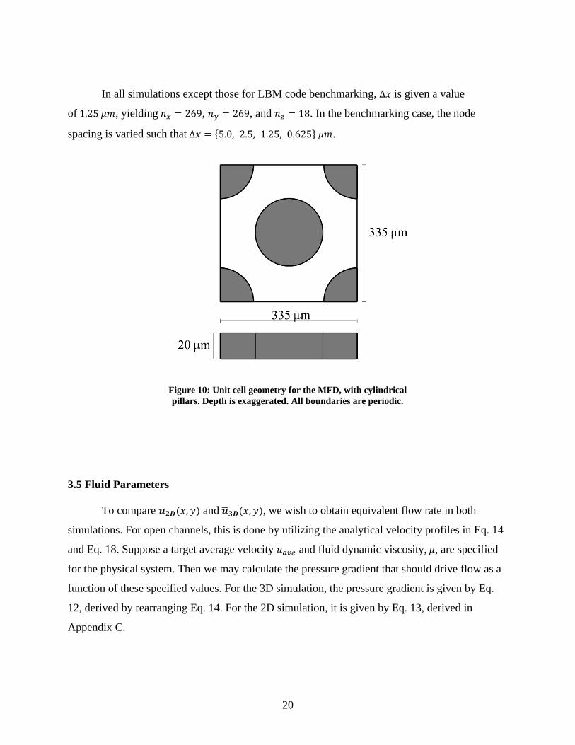
In all simulations except those for LBM code benchmarking, Δ𝑥 is given a value

of 1.25 𝜇𝑚, yielding 𝑛𝑥 = 269, 𝑛𝑦 = 269, and 𝑛𝑧 = 18. In the benchmarking case, the node

spacing is varied such that Δ𝑥 = {5.0, 2.5, 1.25, 0.625} 𝜇𝑚.

3.5 Fluid Parameters

To compare 𝒖𝟐𝟑(𝑥,𝑦) and 𝒖�𝟑𝟑(𝑥,𝑦), we wish to obtain equivalent flow rate in both

simulations. For open channels, this is done by utilizing the analytical velocity profiles in Eq. 14

and Eq. 18. Suppose a target average velocity 𝑢𝑎𝑎𝑎 and fluid dynamic viscosity, 𝜇, are specified

for the physical system. Then we may calculate the pressure gradient that should drive flow as a

function of these specified values. For the 3D simulation, the pressure gradient is given by Eq.

12, derived by rearranging Eq. 14. For the 2D simulation, it is given by Eq. 13, derived in

Appendix C.

Figure 10: Unit cell geometry for the MFD, with cylindrical pillars. Depth is exaggerated. All boundaries are periodic.

21

𝑑𝑑𝑑𝑥

=3𝑢𝑎𝑎𝑎𝜇𝑎2

�192𝑤𝜋5ℎ

� �tanh �𝑖𝜋ℎ2𝑤�

𝑖5� − 1

∞

𝑖=1,3,…

�

−1

Eq. 12

𝑑𝑑𝑑𝑥

=6𝑘1𝑤𝑢𝑎𝑎𝑎𝜇

ℎ2�(1 − 𝑘2)𝑒𝑘2 − (1 + 𝑘2)𝑒−𝑘2

𝑒𝑘2 + 𝑒−𝑘2�−1

Eq. 13

𝑘1 =

2√3ℎ

𝑘2 =𝑘1𝑤

2

Pressure gradients are represented in the simulation as a constant body force driving flow,

necessitating their expression as an acceleration, 𝑎𝑥, for the implementation in Eq. 9. Newton’s

second law of motion relates the pressure gradient and acceleration. Because fluid density, 𝜌, is

given a value of 1.0 in lattice units, the acceleration and pressure gradient are equivalent in the

simulation. Still, it is necessary to convert the pressure gradient from physical to lattice units as

shown earlier.

For cases of variable-depth geometry, the method differs from that of the constant-depth

channel. In particular, it is not known a priori how to specify the pressure gradients in 2D and 3D

such that the same volumetric flow rate is obtained in 𝒖𝟐𝟑(𝑥,𝑦) and 𝒖�𝟑𝟑(𝑥,𝑦). Therefore, 2D and

3D flow is driven with the same pressure gradient. After convergence, 𝒖𝟐𝟑(𝑥,𝑦) is scaled

uniformly such that its volumetric flow rate at the inlet is equal to that of 𝒖�𝟑𝟑(𝑥, 𝑦) at the inlet.

The scale factor is the ratio of the two flow rates, as shown below. Inlet flow rates are

determined by numerically evaluating the integrals below with the composite trapezoidal

approximation.

𝐹𝑥 =

𝑑𝑑𝑑𝑥

𝑉 = 𝑚𝑎𝑥

𝑑𝑑𝑑𝑥

= 𝜌𝑎𝑥

𝑎𝑥 =

1𝜌𝑑𝑑𝑑𝑥

22

Scaling is justified by linearity of the governing equations, the steady-state Stokes

equations. Because any scaling of the pressure gradient will scale the velocity field identically,

scaling the velocity field following convergence is equivalent to scaling the pressure gradient

prior to simulation.

3.6 Boundary Conditions

The inlet and outlet boundaries, i.e. the planes 𝑥 = ±𝑙/2 are periodic in all simulations.

The side boundaries, planes 𝑦 = ±𝑤/2, are also periodic in all simulations except for the

purposes of benchmarking the flow code, where they are no-slip boundaries, as required by the

analytical velocity profiles. The top and bottom boundaries, planes 𝑧 = ±ℎ/2, are no-slip in all

cases.

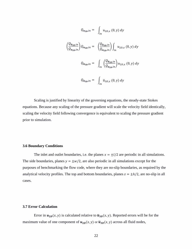
3.7 Error Calculation

Error in 𝒖𝟐𝟑(𝑥,𝑦) is calculated relative to 𝒖�𝟑𝟑(𝑥,𝑦). Reported errors will be for the

maximum value of one component of 𝒖𝟐𝟑(𝑥, 𝑦) or 𝒖�𝟑𝟑(𝑥, 𝑦) across all fluid nodes,

𝑄𝒖𝟐𝟑,𝑖𝑛 = � 𝑢2𝐷,𝑥 (0,𝑦) 𝑑𝑦

𝑖𝑛

�𝑄𝒖�𝟑𝟑,𝑖𝑛

𝑄𝒖𝟐𝟑,𝑖𝑛�𝑄𝒖𝟐𝟑,𝑖𝑛 = �

𝑄𝒖�𝟑𝟑,𝑖𝑛

𝑄𝒖𝟐𝟑,𝑖𝑛�� 𝑢2𝐷,𝑥 (0,𝑦) 𝑑𝑦

𝑖𝑛

𝑄𝒖�𝟑𝟑,𝑖𝑛 = � �

𝑄𝒖�𝟑𝟑,𝑖𝑛

𝑄𝒖𝟐𝟑,𝑖𝑛� 𝑢2𝐷,𝑥 (0,𝑦) 𝑑𝑦

𝑖𝑛

𝑄𝒖�𝟑𝟑,𝑖𝑛 = � 𝑢�3𝐷,𝑥 (0,𝑦) 𝑑𝑦

𝑖𝑛

23

denoted max𝑢𝑖∗, or the average value of one component across all fluid nodes, denoted ⟨𝑢𝑖∗⟩. In

the equations below, 𝑖 = 𝑥 represents the streamwise component and 𝑖 = 𝑦 represents the

transverse component.

𝐸𝑖 =max 𝑢2𝐷,𝑖 − max 𝑢�3𝐷,𝑖

max 𝑢�3𝐷,𝑖× 100%

𝐸𝑖 =⟨𝑢2𝐷,𝑖⟩ − ⟨𝑢�3𝐷,𝑖⟩

⟨𝑢�3𝐷,𝑖⟩× 100%

24

CHAPTER 4: RESULTS

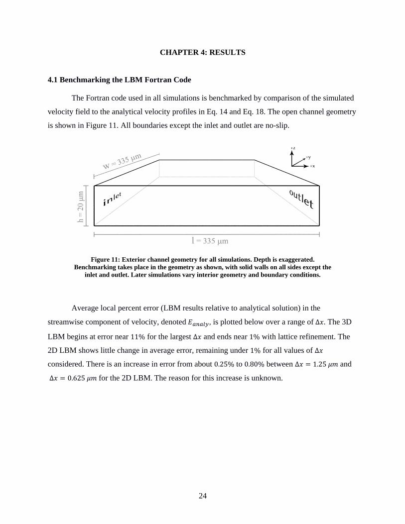
4.1 Benchmarking the LBM Fortran Code

The Fortran code used in all simulations is benchmarked by comparison of the simulated

velocity field to the analytical velocity profiles in Eq. 14 and Eq. 18. The open channel geometry

is shown in Figure 11. All boundaries except the inlet and outlet are no-slip.

Average local percent error (LBM results relative to analytical solution) in the

streamwise component of velocity, denoted 𝐸𝑎𝑛𝑎𝑙𝑦, is plotted below over a range of Δ𝑥. The 3D

LBM begins at error near 11% for the largest Δ𝑥 and ends near 1% with lattice refinement. The

2D LBM shows little change in average error, remaining under 1% for all values of Δ𝑥

considered. There is an increase in error from about 0.25% to 0.80% between Δ𝑥 = 1.25 𝜇𝑚 and

Δ𝑥 = 0.625 𝜇𝑚 for the 2D LBM. The reason for this increase is unknown.

Figure 11: Exterior channel geometry for all simulations. Depth is exaggerated. Benchmarking takes place in the geometry as shown, with solid walls on all sides except the

inlet and outlet. Later simulations vary interior geometry and boundary conditions.

25

4.2 Rapid Symmetric Contracting-Expanding Channel (RSCEC)

Flow is simulated in a rapidly contracting-expanding channel with a centered constriction

formed by symmetric steps, with the purpose of testing 𝒖𝟐𝟑(𝑥,𝑦) with rapid, symmetric depth

variation. The height of each step is one quarter of the total channel depth, or 5 𝜇𝑚. The steps

span the middle one-half of the channel length and the entire width. Flow is driven from left to

right in Figure 13.

Figure 12: Average local error of 2D and 3D LBM velocity relative to analytical solutions for flow in an open rectangular

channel. Average is taken over all fluid nodes. Lattice node spacing is varied between 5 and 0.625 micrometers.

26

The 3D velocity field 𝒖𝟑𝟑(𝑥, 𝑦, 𝑧) in this geometry has nonzero streamwise and vertical

components, and zero transverse component. As previously noted, the vertical component of

𝒖𝟑𝟑(𝑥,𝑦, 𝑧) is omitted from depth-averaging, leaving only the streamwise component nonzero

in 𝒖�𝟑𝟑(𝑥, 𝑦). Because the same is true of 𝒖𝟐𝟑(𝑥, 𝑦), it suffices to compare one-dimensional (1D)

velocity profiles of the streamwise component averaged over the channel width. Note there is

little variability over the width due to the periodic boundaries at 𝑦 = ±𝑤/2. Still, 𝒖�𝟑𝟑(𝑥,𝑦) and

𝒖𝟐𝟑(𝑥,𝑦) are width-averaged and compared in Figure 14. The 1D velocity profiles show

qualitatively good agreement between the two methods with absolute error less than 1%,

implying the assumption of a parabolic velocity profile in the vertical is fairly accurate, as

verified by inspection in Figure 15. Table 1 contains maximum and average values of the

streamwise component of velocity for both 𝒖𝟐𝟑(𝑥,𝑦) and 𝒖�𝟑𝟑(𝑥,𝑦). In both cases, 𝒖𝟐𝟑(𝑥,𝑦)

underestimates 𝒖�𝟑𝟑(𝑥,𝑦) by less than one percent. The Reynolds number (𝑅𝑒) is also included in

Table 1 to demonstrate the assumption of Stokes flow is satisfied. In this case, the characteristic

length scale is twice the average channel depth ℎ�.

Figure 13: The rapid symmetric contracting-expanding channel (RSCEC) geometry. Centered steps reduce channel depth by half. Flow is driven from left to right.

27

Table 1: Streamwise component summary for the RSCEC. Maximum and average values of the streamwise (𝑥) velocity component are reported, in

addition to the 𝑹𝒆 in each simulation. Velocity in units of 𝝁𝝁/𝒔.

max 𝑢𝑥∗ ⟨𝑢𝑥∗ ⟩ 𝑅𝑒 = 2⟨𝑢𝑥∗ ⟩ℎ� 𝜈⁄

𝒖𝟐𝟑 2.908 2.178 6.507 × 10−5

𝒖�𝟑𝟑 2.914 2.181 6.517 × 10−5

𝐸𝑥[%] −0.216 −0.142

Figure 14: Width-averaged velocity profiles of the streamwise component of 𝒖�𝟑𝟑 and 𝒖𝟐𝟑 in the rapid symmetric contracting-

expanding channel.

28

As previously discussed, the implicit depth with 𝒖𝟐𝟑(𝑥,𝑦) may allow for more accurate

determination of the velocity field in narrow constrictions across the channel depth, where

𝒖�𝟑𝟑(𝑥,𝑦) will produce inaccurate results with less than four fluid nodes. To demonstrate, we

perform additional experiments in the RSCEC geometry. The results in Figure 14 and Table 1

were obtained by allowing the steps to block half the channel depth, leaving eight fluid nodes

(𝑛 = 8) or a physical length of 10 𝜇𝑚 within the constriction, whether it be explicitly or

implicitly defined. We reduce the number of fluid nodes in the constriction to test the accuracy

of both approaches, i.e. where 𝒖�𝟑𝟑(𝑥,𝑦) and 𝒖𝟐𝟑(𝑥,𝑦) diverge or converge to an unrealistic result.

Recall that in Figure 14, the streamwise component of velocity approximately doubles within the

constriction, where the depth has been halved. In general, the ratio of the streamwise component

in the constriction to that outside (𝑅𝒖∗) equals the ratio of the depth outside the constriction to

that inside (𝑅ℎ). As seen in Figure 14, velocity is constant within the constriction and outside it.

The results are summarized in Table 2 and plotted in Figure 16.

Figure 15: Profiles of the streamwise velocity component across the channel depth near the constriction in the RSCEC geometry. Profiles follow an approximately parabolic shape.

29

Table 2: Ratio of depth (𝑅ℎ) and streamwise velocity component (𝑅𝒖∗) change due to flow constriction in RSCEC

geometry. Velocity ratio is streamwise component inside constriction to that outside. Depth ratio is depth outside

constriction to that inside. The number of fluid nodes within the constriction is 𝒏.

𝑅ℎ 𝑅𝒖∗

𝑛 = 8 (10 𝜇𝑚)

𝒖𝟐𝟑 2 2.0008

𝒖�𝟑𝟑 2 2.005

𝑛 = 6 (7.5 𝜇𝑚)

𝒖𝟐𝟑 2.67 2.6706

𝒖�𝟑𝟑 2.67 2.6871

𝑛 = 4 (5 𝜇𝑚)

𝒖𝟐𝟑 4 4.0181

𝒖�𝟑𝟑 4 4.1301

𝑛 = 2 (2.5 𝜇𝑚)

𝒖𝟐𝟑 8 8.3411

𝒖�𝟑𝟑 8 12.3643

𝑛 = 1 (1.25 𝜇𝑚)

𝒖𝟐𝟑 16 23.1739

𝒖�𝟑𝟑 16 −0.2162

30

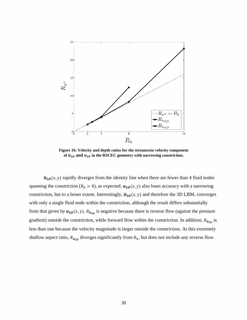
𝒖�𝟑𝟑(𝑥,𝑦) rapidly diverges from the identity line when there are fewer than 4 fluid nodes

spanning the constriction (𝑅ℎ > 4), as expected. 𝒖𝟐𝟑(𝑥, 𝑦) also loses accuracy with a narrowing

constriction, but to a lesser extent. Interestingly, 𝒖�𝟑𝟑(𝑥,𝑦) and therefore the 3D LBM, converges

with only a single fluid node within the constriction, although the result differs substantially

from that given by 𝒖𝟐𝟑(𝑥, 𝑦). 𝑅𝒖�𝟑𝟑 is negative because there is reverse flow (against the pressure

gradient) outside the constriction, while forward flow within the constriction. In addition, 𝑅𝒖�𝟑𝟑 is

less than one because the velocity magnitude is larger outside the constriction. At this extremely

shallow aspect ratio, 𝑅𝒖𝟐𝟑 diverges significantly from 𝑅ℎ, but does not include any reverse flow.

Figure 16: Velocity and depth ratios for the streamwise velocity component of 𝒖�𝟑𝟑 and 𝒖𝟐𝟑 in the RSCEC geometry with narrowing constriction.

31

4.3 Rapid Asymmetric Contracting-Expanding Channel (RACEC)

The RACEC geometry is equivalent to the RSCEC geometry in depth variation; one-half

the depth is blocked within the centered constriction. This geometry differs in that the depth

variation is imposed asymmetrically, with the purpose of testing 𝒖𝟐𝟑(𝑥,𝑦) with rapid,

asymmetric depth variation.

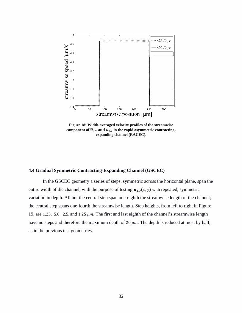
Figure 18 plots the 1D width-averaged velocity profiles of the streamwise component of

𝒖𝟐𝟑(𝑥,𝑦) and 𝒖�𝟑𝟑(𝑥,𝑦). The velocity profiles appear nearly identical to those in Figure 14, for

the RSCEC. The maximum and average values of the streamwise component, however, show

slightly larger error compared to the previous test geometry. The added error may be attributed to

asymmetric depth variation, that being the only difference between the two geometries. Recall

the assumption of a parabolic velocity profile across the channel depth implies the assumption of

symmetry across the horizontal plane. The RACEC clearly violates this assumption, which may

explain the greater error compared to the RSCEC. As in the previous test geometry, 𝒖𝟐𝟑(𝑥,𝑦)

underestimates 𝒖�𝟑𝟑(𝑥,𝑦) in both average and maximum value of the streamwise component.

Table 3: Streamwise component summary for the rapid asymmetric contracting-expanding channel (RACEC). Maximum and average values of the streamwise (𝑥) velocity component are reported, in addition to the 𝑹𝒆 in each simulation. Velocity in units of 𝝁𝝁/𝒔.

max 𝑢𝑥∗ ⟨𝑢𝑥∗ ⟩ 𝑅𝑒 = 2⟨𝑢𝑥∗ ⟩ℎ� 𝜈⁄

𝒖𝟐𝟑 2.860 2.141 6.406 × 10−5

𝒖�𝟑𝟑 2.865 2.144 6.416 × 10−5

𝐸𝑥[%] −0.220 −0.145

Figure 17: The rapid asymmetric contracting-expanding channel (RACEC).

32

4.4 Gradual Symmetric Contracting-Expanding Channel (GSCEC)

In the GSCEC geometry a series of steps, symmetric across the horizontal plane, span the

entire width of the channel, with the purpose of testing 𝒖𝟐𝟑(𝑥,𝑦) with repeated, symmetric

variation in depth. All but the central step span one-eighth the streamwise length of the channel;

the central step spans one-fourth the streamwise length. Step heights, from left to right in Figure

19, are 1.25, 5.0, 2.5, and 1.25 𝜇𝑚. The first and last eighth of the channel’s streamwise length

have no steps and therefore the maximum depth of 20 𝜇𝑚. The depth is reduced at most by half,

as in the previous test geometries.

Figure 18: Width-averaged velocity profiles of the streamwise component of 𝒖�𝟑𝟑 and 𝒖𝟐𝟑 in the rapid asymmetric contracting-

expanding channel (RACEC).

33

Again, it suffices to compare 1D width-averaged velocity profiles. Figure 20 shows

strong agreement between 𝒖𝟐𝟑(𝑥,𝑦) and 𝒖�𝟑𝟑(𝑥, 𝑦). Table 4 reports the maximum and average

value of the streamwise component of velocity. In both cases, 𝒖𝟐𝟑(𝑥,𝑦) underestimates 𝒖�𝟑𝟑(𝑥, 𝑦)

by less than one percent. The same measures of error were greater in both the RSCEC and

RACEC geometries, possibly due to the more rapid depth variation. Recall the underlying

assumption in obtaining 𝒖𝟐𝟑(𝑥,𝑦) that the velocity profile across the implicit channel depth is

parabolic. This assumption derived from considering flow in a constant-depth channel. As we

stray from constant depth by varying the depth more severely, it is reasonable to expect the

assumption of a parabolic profile to be violated, resulting in greater error.

Figure 19: The gradual symmetric contracting-expanding channel (GSCEC).

Figure 20: Width-averaged velocity profiles of the streamwise component of 𝒖�𝟑𝟑 and 𝒖𝟐𝟑 in the gradual symmetric

contracting-expanding channel (GSCEC).

34

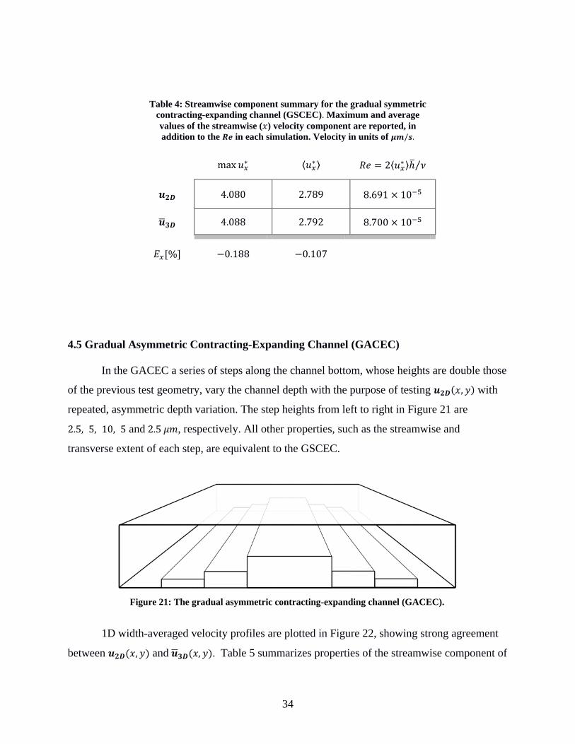
4.5 Gradual Asymmetric Contracting-Expanding Channel (GACEC)

In the GACEC a series of steps along the channel bottom, whose heights are double those

of the previous test geometry, vary the channel depth with the purpose of testing 𝒖𝟐𝟑(𝑥,𝑦) with repeated, asymmetric depth variation. The step heights from left to right in Figure 21 are

2.5, 5, 10, 5 and 2.5 𝜇𝑚, respectively. All other properties, such as the streamwise and

transverse extent of each step, are equivalent to the GSCEC.

1D width-averaged velocity profiles are plotted in Figure 22, showing strong agreement

between 𝒖𝟐𝟑(𝑥,𝑦) and 𝒖�𝟑𝟑(𝑥, 𝑦). Table 5 summarizes properties of the streamwise component of

Table 4: Streamwise component summary for the gradual symmetric contracting-expanding channel (GSCEC). Maximum and average values of the streamwise (𝑥) velocity component are reported, in addition to the 𝑹𝒆 in each simulation. Velocity in units of 𝝁𝝁/𝒔.

max 𝑢𝑥∗ ⟨𝑢𝑥∗ ⟩ 𝑅𝑒 = 2⟨𝑢𝑥∗ ⟩ℎ� 𝜈⁄

𝒖𝟐𝟑 4.080 2.789 8.691 × 10−5

𝒖�𝟑𝟑 4.088 2.792 8.700 × 10−5

𝐸𝑥[%] −0.188 −0.107

Figure 21: The gradual asymmetric contracting-expanding channel (GACEC).

35

velocity, as in previous test cases. 𝒖𝟐𝟑(𝑥,𝑦) underestimates 𝒖�𝟑𝟑(𝑥, 𝑦) by less than one percent in

both maximum and average values.

We now summarize the results of the four contracting-expanding channel geometries.

The error in ⟨𝑢𝑥∗ ⟩ for each is reported in Table 6. All are negative, suggesting 𝒖𝟐𝟑(𝑥, 𝑦) has a bias

toward underestimating 𝒖�𝟑𝟑(𝑥,𝑦) in this general type of geometry. Rapid and asymmetric depth

Table 5: Streamwise component summary for the gradual asymmetric contracting-expanding channel (GACEC). Maximum and average values of both streamwise (𝑥) and transverse (𝑦) velocity components are reported,

in addition to the 𝑹𝒆 in each simulation. Velocity in units of 𝝁𝝁/𝒔.

max 𝑢𝑥∗ ⟨𝑢𝑥∗ ⟩ 𝑅𝑒 = 2⟨𝑢𝑥∗ ⟩ℎ� 𝜈⁄

𝒖𝟐𝟑 4.005 2.738 8.530 × 10−5

𝒖�𝟑𝟑 4.012 2.741 8.540 × 10−5

𝐸𝑥[%] −0.192 −0.113

Figure 22: Width-averaged velocity profiles of the streamwise component of 𝒖�𝟑𝟑 and 𝒖𝟐𝟑 in the gradual

asymmetric contracting-expanding channel (GACEC).

36

variation result in greater absolute error compared to gradual and symmetric depth variation,

respectively. This result is likely due to decreasing accuracy of the underlying assumption used

in obtaining 𝒖𝟐𝟑(𝑥, 𝑦), namely a parabolic velocity profile across the channel vertical. Also, a

change from gradual to rapid depth variation results in greater added error than a change from

symmetric to asymmetric variation. This result suggests the underlying assumption is violated

more severely with the rate of depth variation than its symmetry.

4.6 Constant-Depth Channel with Complete Cylindrical Pillar (CCP)

A single cylindrical pillar is centered in a constant-depth channel. The pillar’s diameter

spans one-half the channel’s streamwise length and width, and its height spans the entire channel

depth. Unlike the previous four geometries, this will test 𝒖𝟐𝟑(𝑥,𝑦) with both components of

velocity being nonzero in the horizontal plane.

Streamlines are plotted in Figure 24 to qualitatively compare 𝒖𝟐𝟑(𝑥,𝑦) and 𝒖�𝟑𝟑(𝑥, 𝑦). The

two sets of streamlines begin to separate near the streamwise front end of the cylinder, and rejoin

Table 6: Summary of contracting-expanding channels: reported values are percent error in ⟨𝑢𝑥∗⟩.

symmetric asymmetric

rapid −0.142 −0.145

Gradual −0.107 −0.113

Figure 23: The constant-depth channel with complete cylindrical pillar (CCP).

37

near the streamwise back end. This characteristic is explained by the left and right periodic

boundaries as well as the geometry’s symmetry. Streamlines near the cylinder appear to separate

more than those further away. This property is explained by considering the differences in each

component of velocity, reported in

Table 7. Note the numbers reported in

Table 7 for the transverse component take its absolute value because there is both positive

and negative transverse flow in this geometry, unlike any of the previous. The transverse

component shows larger absolute error in both maximum and average values over all fluid nodes.

Transverse flow is greatest near the cylinder, particularly near its streamwise front and back,

coinciding with the largest separation in streamlines.

Figure 24: Streamlines of flow around a complete cylinder pillar.

38

In general, 𝒖𝟐𝟑(𝑥,𝑦) overestimates the streamwise component and underestimates the

transverse component. The average values for both velocity components show good agreement

between 𝒖𝟐𝟑(𝑥,𝑦) and 𝒖�𝟑𝟑(𝑥, 𝑦), with less than one percent difference, while the maximum

values show the largest absolute errors so far. The average of the transverse component is

underestimated by about two orders of magnitude greater than the streamwise component is

overestimated. Similarly, the transverse component’s maximum is underestimated more severely

than the streamwise component’s maximum is overestimated.

Table 7 also reports the Reynolds number for each flow, defined with the average velocity

magnitude ⟨‖𝒖∗‖⟩ and cylinder diameter 𝑑.

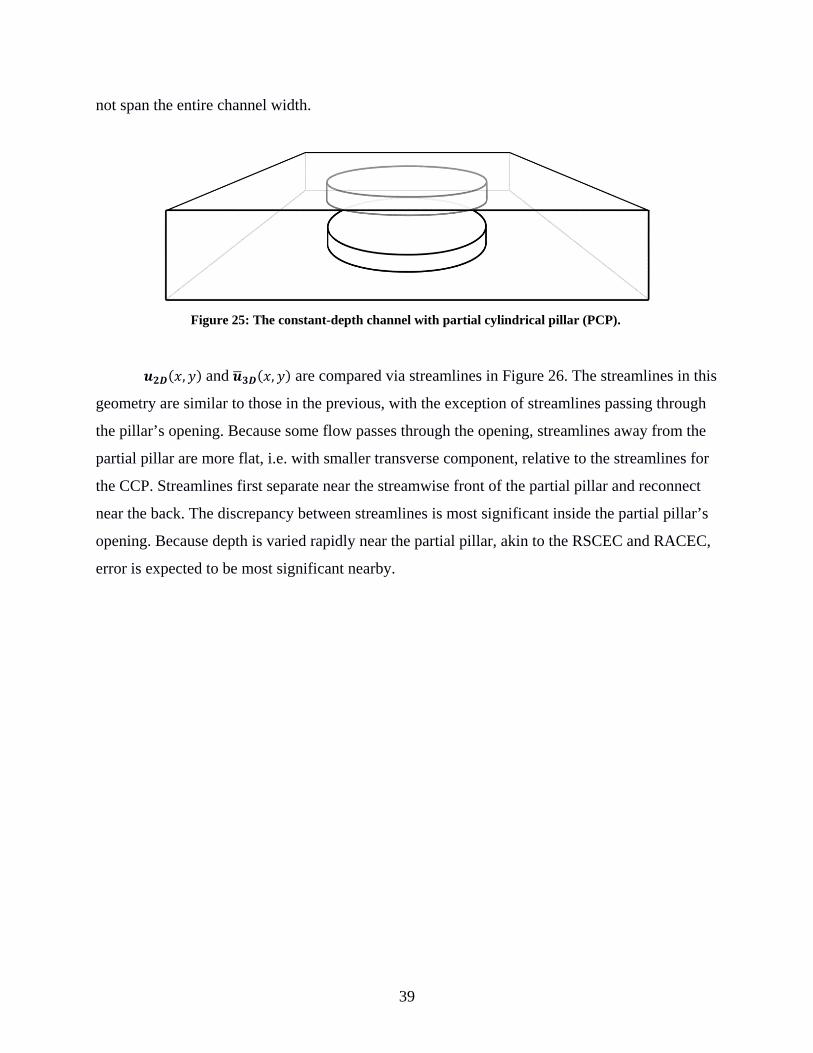
4.7 Constant-depth Channel with Partial Cylindrical Pillar (PCP)

Flow is simulated in a geometry similar to the CCP, except the cylindrical pillar does not

span the entire channel depth. Instead, the middle one-half of the pillar’s height is removed. The

partial pillar is centered in the channel and has a diameter spanning one-half the channel’s length

and width. This geometry will test 𝒖𝟐𝟑(𝑥,𝑦) with two nonzero components of velocity in the

horizontal plane with depth variation, unlike the previous test geometries. Note that unlike in the

CCP test case, the 2D geometry here does not include a cylindrical pillar. This geometry is

similar to the contracting-expanding channels examined earlier, except the step constriction does

Table 7: Velocity field summary for the complete cylindrical pillar (CCP). Maximum and average

values of both streamwise (𝑥) and transverse (𝑦) velocity components are reported, in addition to the 𝑹𝒆 in each simulation. Velocity in units of 𝝁𝝁/𝒔.

max 𝑢𝑥∗ ⟨𝑢𝑥∗ ⟩ max�𝑢𝑦∗ � ⟨�𝑢𝑦∗ �⟩ 𝑅𝑒 = ⟨‖𝒖∗‖⟩𝑑 𝜈⁄

𝒖𝟐𝟑 10.212 4.2705 2.841 0.810 7.382 × 10−4

𝒖�𝟑𝟑 9.716 4.2702 3.790 0.817 7.401 × 10−4

𝐸𝑖[%] 5.11 0.00703 −25.0 −0.850

39

not span the entire channel width.

𝒖𝟐𝟑(𝑥,𝑦) and 𝒖�𝟑𝟑(𝑥, 𝑦) are compared via streamlines in Figure 26. The streamlines in this

geometry are similar to those in the previous, with the exception of streamlines passing through

the pillar’s opening. Because some flow passes through the opening, streamlines away from the

partial pillar are more flat, i.e. with smaller transverse component, relative to the streamlines for

the CCP. Streamlines first separate near the streamwise front of the partial pillar and reconnect

near the back. The discrepancy between streamlines is most significant inside the partial pillar’s

opening. Because depth is varied rapidly near the partial pillar, akin to the RSCEC and RACEC,

error is expected to be most significant nearby.

Figure 25: The constant-depth channel with partial cylindrical pillar (PCP).

40

Both components of the velocity field are reported in Table 8. The closest agreement

between 𝒖𝟐𝟑(𝑥,𝑦) and 𝒖�𝟑𝟑(𝑥,𝑦) is in the average streamwise component, in line with previous

results. The average streamwise component is overestimated by 𝒖𝟐𝟑(𝑥, 𝑦); all other metrics

considered in the table are underestimated. The absolute errors in maximum and average

transverse component are larger than those for the streamwise component, also in line with

Table 8: Velocity field summary for the partial cylindrical pillar (PCP). Maximum and average values of both streamwise (𝑥) and transverse (𝑦) velocity components are reported, in addition to the 𝑹𝒆 in

each simulation. Velocity in units of 𝝁𝝁/𝒔.

max 𝑢𝑥∗ ⟨𝑢𝑥∗ ⟩ max�𝑢𝑦∗ � ⟨�𝑢𝑦∗ �⟩ 𝑅𝑒 = ⟨‖𝒖∗‖⟩𝑑 𝜈⁄

𝒖𝟐𝟑 8.723 4.966 2.179 0.657 8.426 × 10−4

𝒖�𝟑𝟑 9.306 4.874 3.286 0.714 8.322 × 10−4

𝐸𝑖[%] −6.26 1.88 −33.7 −7.94

Figure 26: Streamlines of flow around and through a partial cylindrical pillar.

41

previous results. The absolute errors reported in Table 8 are the largest yet, which is reasonable

considering the flow is the most complex yet.

4.8 Constant-Depth Unit Cell (UC)

The unit cell is a representative section of the MFD, depicted in Figure 27. It contains a

central cylindrical pillar and a quarter pillar centered on each vertical edge of the domain. All

pillars span the entire channel depth. The unit cell geometry will test 𝒖𝟐𝟑(𝑥,𝑦) with a more

complex flow in the horizontal plane, relative to the CCP geometry, with no vertical component

of velocity because the channel depth is constant.

Streamlines for 𝒖𝟐𝟑(𝑥, 𝑦) and 𝒖�𝟑𝟑(𝑥,𝑦) are plotted in Figure 28. In the two previous test

cases, streamlines matched well away from the central pillar. This is not the case in the unit cell

geometry. Streamlines show their maximum separation away from the central pillar. As noted

earlier, streamlines appear to separate in regions of significant transverse flow. Pillars on each

corner of the plane result in significant transverse flow throughout nearly the entire domain,

except near the top and bottom edges, where the streamlines agree relatively well. Symmetry in

the horizontal plane results in streamlines that begin and end in agreement. Suppose the

Figure 27: The constant-depth unit cell geometry (planar view).

42

geometry was not symmetric in the horizontal plane. Then the discrepancy in streamlines

produced in the left half plane may not “reverse” itself in the right half plane. Therefore, it is

possible in simulating flow in an irregular geometry that early error, characterized by streamline

discrepancy, could propagate and increase downstream. We note this possibility as a

consideration for applying and extending the current work.

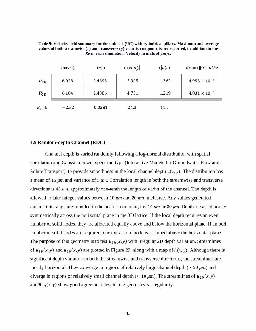
Properties of the velocity components are summarized in Table 9. The best agreement

between 𝒖𝟐𝟑(𝑥,𝑦) and 𝒖�𝟑𝟑(𝑥,𝑦) is in the average streamwise component of velocity, where the

error is less than one percent. The maximum of the streamwise component is underestimated

by 𝒖𝟐𝟑(𝑥, 𝑦), while all other metrics considered in the table are overestimated. As before, the

streamwise component of 𝒖�𝟑𝟑(𝑥,𝑦) is better approximated by 𝒖𝟐𝟑(𝑥,𝑦) than the transverse

component.

Figure 28: Streamline comparison for flow in the unit cell.

43

4.9 Random-depth Channel (RDC)

Channel depth is varied randomly following a log-normal distribution with spatial

correlation and Gaussian power spectrum type (Interactive Models for Groundwater Flow and

Solute Transport), to provide smoothness in the local channel depth ℎ(𝑥, 𝑦). The distribution has

a mean of 15 𝜇𝑚 and variance of 5 𝜇𝑚. Correlation length in both the streamwise and transverse

directions is 40 𝜇𝑚, approximately one-tenth the length or width of the channel. The depth is

allowed to take integer values between 10 𝜇𝑚 and 20 𝜇𝑚, inclusive. Any values generated

outside this range are rounded to the nearest endpoint, i.e. 10 𝜇𝑚 or 20 𝜇𝑚. Depth is varied nearly

symmetrically across the horizontal plane in the 3D lattice. If the local depth requires an even

number of solid nodes, they are allocated equally above and below the horizontal plane. If an odd

number of solid nodes are required, one extra solid node is assigned above the horizontal plane.

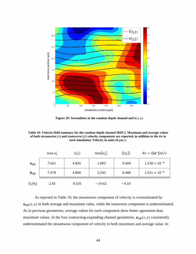
The purpose of this geometry is to test 𝒖𝟐𝟑(𝑥,𝑦) with irregular 2D depth variation. Streamlines

of 𝒖𝟐𝟑(𝑥,𝑦) and 𝒖�𝟑𝟑(𝑥,𝑦) are plotted in Figure 29, along with a map of ℎ(𝑥, 𝑦). Although there is

significant depth variation in both the streamwise and transverse directions, the streamlines are

mostly horizontal. They converge in regions of relatively large channel depth (≈ 20 𝜇𝑚) and

diverge in regions of relatively small channel depth (≈ 10 𝜇𝑚). The streamlines of 𝒖𝟐𝟑(𝑥, 𝑦)

and 𝒖�𝟑𝟑(𝑥,𝑦) show good agreement despite the geometry’s irregularity.

Table 9: Velocity field summary for the unit cell (UC) with cylindrical pillars. Maximum and average values of both streamwise (𝑥) and transverse (𝑦) velocity components are reported, in addition to the

𝑹𝒆 in each simulation. Velocity in units of 𝝁𝝁/𝒔.

max 𝑢𝑥∗ ⟨𝑢𝑥∗ ⟩ max�𝑢𝑦∗ � ⟨�𝑢𝑦∗ �⟩ 𝑅𝑒 = ⟨‖𝒖∗‖⟩𝑑 𝜈⁄

𝒖𝟐𝟑 6.028 2.4893 5.905 1.362 4.953 × 10−4

𝒖�𝟑𝟑 6.184 2.4886 4.751 1.219 4.831 × 10−4

𝐸𝑖[%] −2.52 0.0281 24.3 11.7

44

As reported in Table 10, the streamwise component of velocity is overestimated by

𝒖𝟐𝟑(𝑥,𝑦) in both average and maximum value, while the transverse component is underestimated.

As in previous geometries, average values for each component show better agreement than

maximum values. In the four contracting-expanding channel geometries, 𝒖𝟐𝟑(𝑥,𝑦) consistently

underestimated the streamwise component of velocity in both maximum and average value. In

Table 10: Velocity field summary for the random-depth channel (RDC). Maximum and average values of both streamwise (𝑥) and transverse (𝑦) velocity components are reported, in addition to the 𝑹𝒆 in

each simulation. Velocity in units of 𝝁𝝁/𝒔.

max 𝑢𝑥∗ ⟨𝑢𝑥∗ ⟩ max�𝑢𝑦∗ � ⟨�𝑢𝑦∗ �⟩ 𝑅𝑒 = ⟨‖𝒖∗‖⟩𝑑 𝜈⁄

𝒖𝟐𝟑 7.661 4.826 1.803 0.468 1.538 × 10−4

𝒖�𝟑𝟑 7.478 4.800 2.243 0.488 1.531 × 10−4

𝐸𝑖[%] 2.45 0.535 −19.62 −4.10

Figure 29: Streamlines in the random-depth channel and 𝒉(𝒙,𝒚).

45

those cases, the transverse component of velocity was zero. The current geometry has nonzero,

although relatively little, transverse flow, seen by comparing the magnitudes of max 𝑢𝑖∗ and ⟨𝑢𝑖∗⟩.

In the random-depth channel, 𝒖𝟐𝟑(𝑥,𝑦) overestimates the streamwise component in both

maximum and average value, suggesting the negative bias in streamwise component observed in

earlier geometries is dependent on the transverse component.

4.10 Unit Cell with Random Depth (UCRD)

The final geometry is a unit cell with random depth, representative of the expected

geometry in a section of the MFD with significant precipitate accumulation on the top and

bottom surfaces. The depth field ℎ(𝑥,𝑦) used previously in the random-depth channel defines

local depth around the cylindrical pillars. Thus, the current geometry is simply a composition of

the UC and RDC geometries. As before, the channel depth may be constricted by at most one-

half its maximum value.

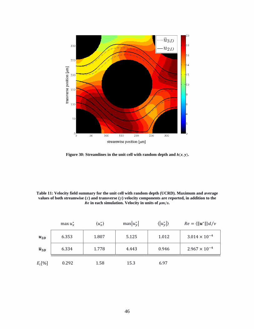
Streamlines of 𝒖𝟐𝟑(𝑥,𝑦) and 𝒖�𝟑𝟑(𝑥,𝑦) are plotted in Figure 30, along with a map

of ℎ(𝑥, 𝑦). The irregular depth results in greater separation of streamlines relative to the unit cell

geometry with constant depth. In addition, streamlines do not converge past the streamwise back

of the central cylinder, as they did in the previous unit cell geometry due to its symmetry. If the

domain were extended further downstream, the discrepancy in streamlines would propagate, and

likely grow with length if the depth continued to be irregular. In general, 𝒖𝟐𝟑(𝑥, 𝑦) may

approximate 𝒖�𝟑𝟑(𝑥,𝑦) more poorly with streamwise length in a realistic, i.e. arbitrary depth,

MFD geometry.

46

Table 11: Velocity field summary for the unit cell with random depth (UCRD). Maximum and average values of both streamwise (𝑥) and transverse (𝑦) velocity components are reported, in addition to the

𝑹𝒆 in each simulation. Velocity in units of 𝝁𝝁/𝒔.

max 𝑢𝑥∗ ⟨𝑢𝑥∗ ⟩ max�𝑢𝑦∗ � ⟨�𝑢𝑦∗ �⟩ 𝑅𝑒 = ⟨‖𝒖∗‖⟩𝑑 𝜈⁄

𝒖𝟐𝟑 6.353 1.807 5.125 1.012 3.014 × 10−4

𝒖�𝟑𝟑 6.334 1.778 4.443 0.946 2.967 × 10−4

𝐸𝑖[%] 0.292 1.58 15.3 6.97

Figure 30: Streamlines in the unit cell with random depth and 𝒉(𝒙,𝒚).

47

𝒖𝟐𝟑(𝑥,𝑦) overestimates 𝒖�𝟑𝟑(𝑥,𝑦) in maximum and average value for both velocity

components. Absolute error is larger for the transverse component, as in all other test geometries

with nonzero transverse flow. Because the current geometry is a composition of two previous

geometries, we compare the errors for each in Table 12. One may expect a worse performance by

𝒖𝟐𝟑(𝑥,𝑦) in the UCRD geometry, compared to the UC or RDC geometries, because it is more

complex. In the average streamwise component, this is the case. In all other metrics considered,

𝒖𝟐𝟑(𝑥,𝑦) performs worst in the UC geometry. Although there appear to be some trends relating

error to geometric features (see the summary of contracting-expanding channel geometries), the

results summarized in Table 12 show that accuracy of 𝒖𝟐𝟑(𝑥,𝑦) in approximating 𝒖�𝟑𝟑(𝑥,𝑦) is not

always a simple function of the geometry complexity.

4.11 Series of Unit Cells with Random Depth (SUCRD)

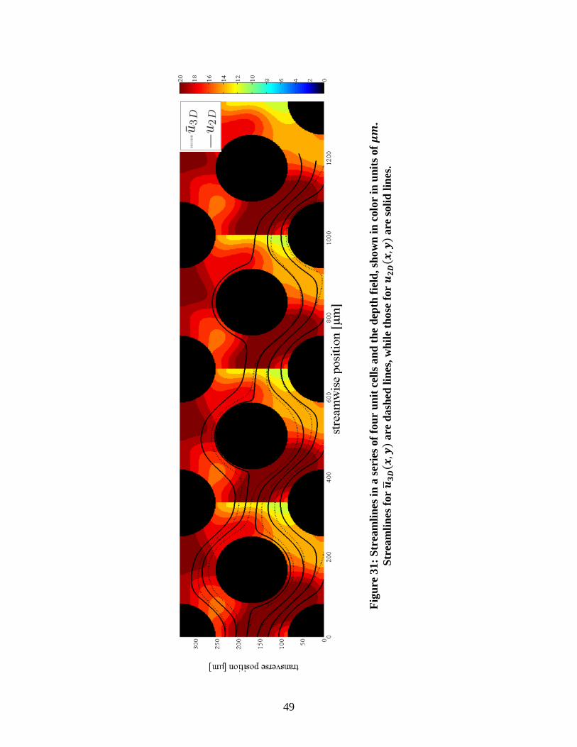
The final test geometry is a series of four unit cells with the purpose of studying

downstream propagation of error between 𝒖𝟐𝟑(𝑥,𝑦) and 𝒖�𝟑𝟑(𝑥, 𝑦). The random spatially-

correlated depth within each cell is identical to that used previously in the RDC and UCRD test

geometries. Although concatenating unit cells results in abrupt depth change at each boundary,

we expect 𝒖𝟐𝟑(𝑥,𝑦) can handle this case considering the previously reported results of the

contracting-expanding channels with rapid depth variation in Sections 4.2 and 4.3. Figure 31

plots streamlines for 𝒖𝟐𝟑(𝑥,𝑦) and 𝒖�𝟑𝟑(𝑥,𝑦) against a map of the local channel depth.

Table 12: Error summary for unit cell (UC), random-depth channel

(RDC), and unit cell with random depth (UCRD) geometries. Reported values are percent error.

max 𝑢𝑥∗ ⟨𝑢𝑥∗ ⟩ max�𝑢𝑦∗ � ⟨�𝑢𝑦∗ �⟩

UC −2.52 0.0281 24.3 11.7

RDC 2.45 0.535 −19.62 −4.10

UCRD 0.292 1.58 15.3 6.97

48

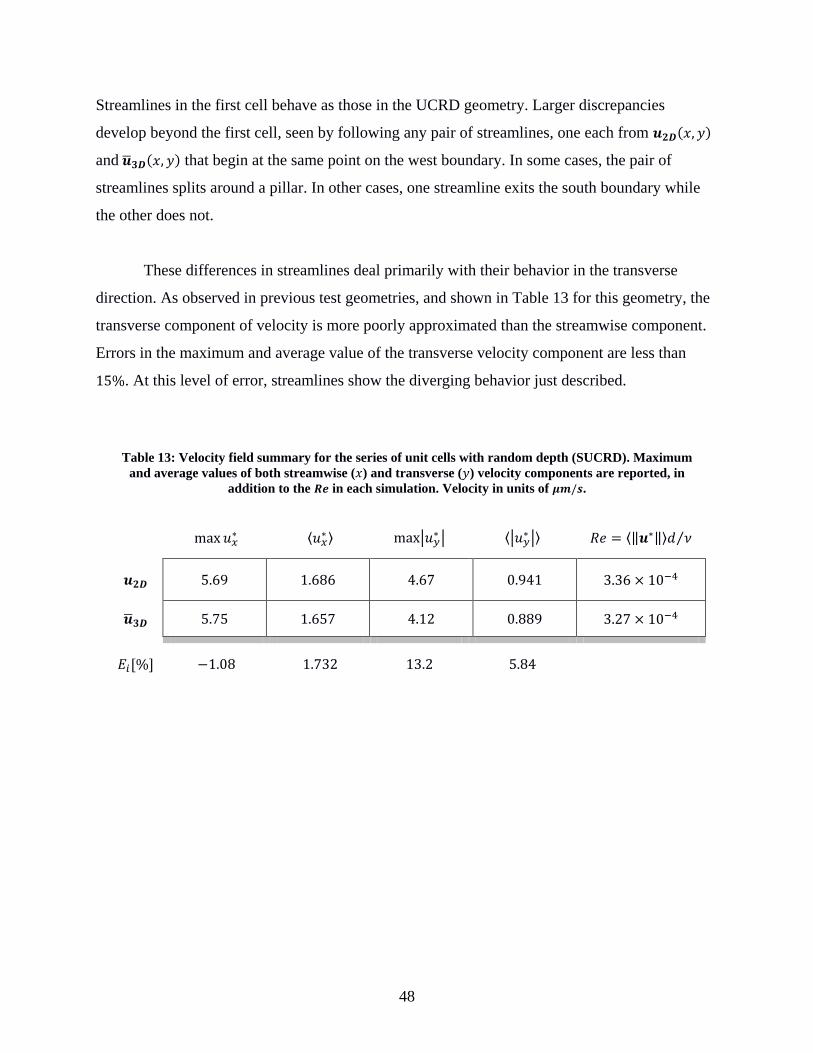
Streamlines in the first cell behave as those in the UCRD geometry. Larger discrepancies

develop beyond the first cell, seen by following any pair of streamlines, one each from 𝒖𝟐𝟑(𝑥,𝑦)

and 𝒖�𝟑𝟑(𝑥,𝑦) that begin at the same point on the west boundary. In some cases, the pair of

streamlines splits around a pillar. In other cases, one streamline exits the south boundary while

the other does not.

These differences in streamlines deal primarily with their behavior in the transverse

direction. As observed in previous test geometries, and shown in Table 13 for this geometry, the

transverse component of velocity is more poorly approximated than the streamwise component.

Errors in the maximum and average value of the transverse velocity component are less than

15%. At this level of error, streamlines show the diverging behavior just described.

Table 13: Velocity field summary for the series of unit cells with random depth (SUCRD). Maximum

and average values of both streamwise (𝑥) and transverse (𝑦) velocity components are reported, in addition to the 𝑹𝒆 in each simulation. Velocity in units of 𝝁𝝁/𝒔.

max 𝑢𝑥∗ ⟨𝑢𝑥∗ ⟩ max�𝑢𝑦∗ � ⟨�𝑢𝑦∗ �⟩ 𝑅𝑒 = ⟨‖𝒖∗‖⟩𝑑 𝜈⁄

𝒖𝟐𝟑 5.69 1.686 4.67 0.941 3.36 × 10−4

𝒖�𝟑𝟑 5.75 1.657 4.12 0.889 3.27 × 10−4

𝐸𝑖[%] −1.08 1.732 13.2 5.84

49

Figu

re 3

1: S

trea

mlin

es in

a se

ries

of f

our

unit

cells

and

the

dept

h fie

ld, s

how

n in

col

or in

uni

ts o

f 𝝁𝝁

. St

ream

lines

for 𝒖� 𝟑

𝟑( 𝒙

,𝒚) a

re d

ashe

d lin

es, w

hile

thos

e fo

r 𝒖 𝟐

𝟑( 𝒙

,𝒚) a

re so

lid li

nes.

50

4.12 Comparison of Run Times

Table 14 reports the run time needed to solve for 𝒖𝟐𝟑(𝑥,𝑦), denoted 𝑅𝑇𝒖𝟐𝟑, the run time

needed to solve for 𝒖�𝟑𝟑(𝑥,𝑦), denoted 𝑅𝑇𝒖�𝟑𝟑, and the ratio of the two, denoted 𝑆, for all ten

geometries. All code is sequential and run on an Intel Core i5-3570 CPU. Repeated runs of the

same simulation yielded run times within one second of each other. This variation has little effect

on the value of 𝑆, so only the times for a single run are reported. 𝑆 ranges from 3.7 to 10.1, with

an average value of 6.9. As a rough approximation, solving the 2D governing equations is about

seven times faster, on average, than solving 3D governing equations, at least across the ten

geometries considered. While the 2D simulations have shorter run times, they require more

iterations to converge. For example, in the GSCEC geometry 𝒖𝟐𝟑(𝑥,𝑦) requires about 13,000

iterations to converge, while 𝒖𝟑𝟑(𝑥,𝑦) requires about 3,000. In the UCRD geometry 𝒖𝟐𝟑(𝑥,𝑦)

requires about 17,000 iterations to converge, while 𝒖𝟑𝟑(𝑥,𝑦) requires about 3,500.

Table 14: Simulation run time for 𝒖𝟐𝟑 (𝑹𝑻𝒖𝟐𝟑) and 𝒖�𝟑𝟑 (𝑹𝑻𝒖�𝟑𝟑) in each test geometry in units of seconds. Ratio of run times 𝑺 = 𝑹𝑻𝒖�𝟑𝟑/𝑹𝑻𝒖𝟐𝟑.

Geometry 𝑅𝑇𝒖𝟐𝟑 𝑅𝑇𝒖�𝟑𝟑 𝑆 = 𝑅𝑇𝒖�𝟑𝟑/𝑅𝑇𝒖𝟐𝟑

RSCEC 49.4 493.9 10.0

RACEC 49.5 498.8 10.1

GSCEC 66.2 403.6 6.1

GACEC 49.4 497.2 10.1

CCP 132.5 656.6 5.0

PCP 155.7 573.5 3.7

UC 82.7 557.5 6.7

RDC 101.8 456.4 4.5

UCRD 62.5 419.4 6.7

SUCRD 294.8 1742.0 5.9

51

4.13 Effects of Velocity Field Scaling and the Viscous Drag Term

Two modifications are made to the standard 2D LBM so that 𝒖𝟐𝟑(𝑥,𝑦) may more closely

approximate 𝒖�𝟑𝟑(𝑥,𝑦). First, 𝒖𝟐𝟑(𝑥,𝑦) is solved for with an external acceleration representing

viscous drag from the top and bottom MFD surfaces. Second, after 𝒖𝟐𝟑(𝑥,𝑦) is solved for it is

uniformly scaled so its inlet flow rate equals that of 𝒖�𝟑𝟑(𝑥,𝑦). The effect of these modifications

is studied by revisiting the unit cell with random depth geometry, shown earlier in Figure 30.

Errors between 𝒖𝟐𝟑(𝑥,𝑦) and 𝒖�𝟑𝟑(𝑥,𝑦) without scaling, without viscous drag, and with neither

scaling nor viscous drag are reported in Table 15. Errors with scaling and viscous drag are

reported again in the first row for comparison. The least absolute error for each category is

marked by an asterisk.

For the maximum and average value of the streamwise component, the least absolute

error comes from omitting the viscous drag term and scaling 𝒖𝟐𝟑(𝑥,𝑦). This result suggests

scaling can account for most of the effect of viscous drag for the streamwise velocity component,

but not for the transverse. The poor agreement in transverse component is seen in Figure 32,

Table 15: Error summary for the unit cell with random depth (UCRD) with and without

scaling and viscous drag. Reported values are percent error of maximum and average values for both streamwise (𝑥) and transverse (𝑦) velocity components. The least absolute error for

each category is marked by an asterisk.

max 𝑢𝑥∗ ⟨𝑢𝑥∗ ⟩ max�𝑢𝑦∗ � ⟨�𝑢𝑦∗ �⟩

𝐸𝑖[%] 0.292 1.58 15.3* 6.97*

𝐸𝑖[%] (no scaling) −40.84 −40.07 −31.95 −36.903

𝐸𝑖[%] (no viscous drag) 0.0647* 0.0321* 31.00 18.515

𝐸𝑖[%] (no scaling or viscous drag)

167 149 208 169

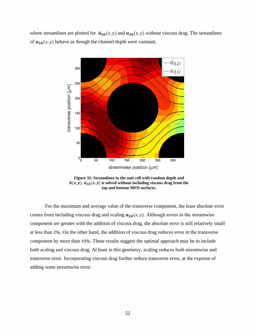
52

where streamlines are plotted for 𝒖�𝟑𝟑(𝑥,𝑦) and 𝒖𝟐𝟑(𝑥,𝑦) without viscous drag. The streamlines

of 𝒖𝟐𝟑(𝑥,𝑦) behave as though the channel depth were constant.

For the maximum and average value of the transverse component, the least absolute error

comes from including viscous drag and scaling 𝒖𝟐𝟑(𝑥,𝑦). Although errors in the streamwise

component are greater with the addition of viscous drag, the absolute error is still relatively small

at less than 2%. On the other hand, the addition of viscous drag reduces error in the transverse

component by more than 10%. These results suggest the optimal approach may be to include

both scaling and viscous drag. At least in this geometry, scaling reduces both streamwise and

transverse error. Incorporating viscous drag further reduce transverse error, at the expense of

adding some streamwise error.

Figure 32: Streamlines in the unit cell with random depth and 𝒉(𝒙,𝒚). 𝒖𝟐𝟑(𝒙,𝒚) is solved without including viscous drag from the

top and bottom MFD surfaces.

53

CHAPTER 5: DISCUSSION

Ten test geometries have been studied to determine if a 2D, depth-averaged LBM can

successfully approximate the depth-averaged results of a 3D LBM to reduce the computational

cost of reactive transport models in MFDs. Existing work in the literature has successfully

implemented this approximation for the case of a constant depth MFD. The method proposed in

this thesis extends that work to cases of spatially-variable depth.

The first four test geometries were variations of an expanding-contracting channel in

which depth varied only in the streamwise direction. These simple geometries discerned the

relative error caused by rapid and asymmetric depth variation, finding the former to be more

significant than the latter. Other test geometries were more complex and included flow around

cylinder pillars and through a channel with randomly-generated depth. The more complex flows

in these geometries resulted in greater discrepancy between the true velocity field and its

approximation.

In general, the streamwise component of velocity was approximated more closely than

the transverse component. This result can be explained, at least in part, by the scaling procedure

implemented to guarantee that velocity fields are compared with equal volumetric flow rate.

Scaling was required because we could not determine, a priori, the driving force (pressure

gradient) needed in paired 2D and 3D simulations to produce equal flow rate; equal driving force

did not produce equal flow rate. Although scaling can be justified for the case of Stokes flow

considered in this work, the need to scale limits application of the proposed method to other

flows.

The 2D, depth-averaged LBM incorporates viscous drag from the horizontally-oriented

top and bottom MFD surfaces by approximating it with an external resistive acceleration.

However, the effect of viscous drag from vertically-oriented solid surfaces, such as the sides of

cylindrical pillars, is not accounted for. The influence of these surfaces on the velocity field

should be studied further to improve accuracy of the 2D approximation.

54

An additional limitation of the proposed approach is the propagation and increase of error

with streamwise length. If streamline separation is an acceptable measure, it seems that in

complex and asymmetric geometries errors in the velocity field will increase with streamwise

length of the simulation domain. This property is problematic for the accuracy of 2D solute

transport and reaction models coupled to the 2D, depth-averaged LBM. Further numerical

experiments in larger and more complex domains are needed to discern the severity of this

potential limitation.

Based on results in the final and most complex test case, the proposed 2D, depth-

averaged approach would not approximate the transport of solutes in a MFD to high accuracy, its

primary shortcoming being poor prediction of transverse flow. However, it is expected to be

more accurate than existing 2D approaches, because it includes some 3D effects. Including

additional 3D effects, such as viscous drag from vertically-oriented surfaces, or utilizing a

different LBM body force implementation, may further increase accuracy. Still, it is likely the

proposed 2D method will provide a rough approximation of reactive transport in complex, 3D

systems. For applications where a rough approximation is sufficient, much computational time

can be saved with a 2D method. For applications requiring higher accuracy, 3D methods should

be employed.

55

BIBLIOGRAPHY

Bhatnagar, P.L., E.P. Gross, and M. Krook. “A Model for Collision Processes in Gases. I. Small

Amplitude Processes in Charged and Neutral One-Component Systems.” Physical Review

94, no. 3 (1954).

Boek, E.S. and M. Venturoli. “Lattice-Boltzmann studies of fluid flow in porous media with

realistic rock geometries.” Computers and Mathematics with Applications 59 (2010): 2305 –

2314.

Flekkoy, E.G., U. Oxaal, J. Feder, and T. Jossang. “Hydrodynamic Dispersion at Stagnation

Points: Simulations and Experiments.” Physical Review E 52, no. 5 (1995).

Guo, Z., C. Zheng, and B. Shi. “Discrete Lattice Effects on the Forcing Term in the Lattice

Boltzmann Method.” Physical Review E 65 (2002).

He, X. and L.S. Luo. “Lattice Boltzmann model for the incompressible Navier-Stokes equations.”

Journal of Statistical Physics 88, (1997).

Interactive Models for Groundwater Flow and Solute Transport. Last modified April 2014,

http://hydrolab.illinois.edu/gw_applets//?q=gw_applets/.

Latt, J. “Choice of units in lattice Boltzmann simulations.” Freely available online

at http://lbmethod.org/_media/howtos:lbunits.pdf. (2008).

Luo, Li-Shi. “Theory of the Lattice Boltzmann Method: Lattice Boltzmann Models for Nonideal

Gases.” Physical Review E 62, no. 4 (2000): 4982.

Mohamad, A.A. and A. Kuzmin. “A Critical Evaluation of Force Term in Lattice Boltzmann

Method, Natural Convection Problem.” International Journal of Heat and Mass Transfer

53 (2010).

Nambi, I.M., C.J. Werth, R.A. Sanford, and A.J. Valocchi. 2003. “Pore-Scale Analysis of

Anaerobic Halorespiring Bacterial Growth Along the Transverse Mixing Zone of an

Etched Silicon Pore Network.” Environ. Sci. Technol. 37: 5617–5624.

Succi, S. The Lattice Boltzmann Equation for Fluid Dynamics and Beyond. Oxford: Clarendon

Press, 2001.

Sukop, M.C. and D.T. Thorne, Jr. Lattice Boltzmann Modeling: An Introduction for

Geoscientists and Engineers. Springer, 2007.

56

Venturoli, M. and E.S. Boek. “Two-dimensional lattice-Boltzmann Simulations of Single Phase

Flow in a Pseudo Two-dimensional Micromodel.” Physica A: Statistical Mechanics and

Its Applications 362, no. 1 (2006): 23–29.

White, F.M. Viscous Fluid Flow. 2nd ed. McGraw-Hill, Inc., 1991.

Willingham, T., C. Zhang, C.J. Werth, A.J. Valocchi, M. Oostrom, and T.W. Wietsma. 2010.

“Using Dispersivity Values to Quantify the Effects of Pore-scale Flow Focusing on

Enhanced Reaction Along a Transverse Mixing Zone.” Advances in Water Resources 33:

525–535.

Willingham, T. W., C. J. Werth, and A. J. Valocchi. “Evaluation of the effects of porous media

structure on mixing-controlled reactions using pore-scale modeling and micromodel

experiments.” Environmental Science & Technology 42, (2008): 3185-3193.

Yoon, H., A. J. Valocchi, C. J. Werth, and T. Dewers. “Pore-scale simulation of mixing-induced

calcium carbonate precipitation and dissolution in a microfluidic pore network.” Water

Resources Research 48, (2012).

Zhang, C., K. Dehoff, T. Wietsma, A. Valocchi, B. Fouke, and C. Werth. “Pore-Scale Study of

Transverse Mixing Induced CaCO3 Precipitation and Permeability Reduction in a Model

Subsurface Sedimentary System.” Environ. Sci. Technol. 44 (2010): 7833–7838. Zou, Q. and X. He. “On Pressure and Velocity Boundary Conditions for the Lattice Boltzmann

BGK Model.” Physics of Fluids 9, no. 6 (1997).

57

APPENDIX A: SUMMARY OF ANALYTICAL SOLUTIONS FOR OPEN,

RECTANGULAR CHANNEL FLOWS

Flow in a 3D channel with rectangular cross section

The steady-state 3D velocity profile, defined over a rectangular cross section such that −𝑤/2 ≤

𝑦 ≤ 𝑤/2 and −ℎ/2 ≤ 𝑧 ≤ ℎ/2, is reported in Eq. 14 (White 1991). 𝑑𝑑/𝑑𝑥 is the pressure gradient

in the streamwise direction, ℎ is the constant channel depth, 𝑤 is the constant channel width, 𝜇 is

the fluid dynamic viscosity, 𝑦 is the transverse spatial coordinate, and 𝑧 is the vertical spatial

coordinate.

𝑢3𝐷,𝑥(𝑦, 𝑧) =4𝑤2

𝜇𝜋3�−

𝑑𝑑𝑑𝑥� � (−1)(𝑖−1)/2 �1 −

cosh (𝑖𝜋𝑧/𝑤)cosh(𝑖𝜋ℎ/2𝑤)

�cos (𝑖𝜋𝑦/𝑤)

𝑖3

∞

𝑖=1,3,…

Eq. 14

Integrating the velocity profile over the cross section yields the volumetric flow rate (𝑄),

reported in Eq. 15 (White 1991). Note the flow rate is equivalent to the average streamwise

velocity (𝑢𝑎𝑎𝑎) multiplied by the cross-sectional area (𝐴 = 𝑤ℎ).

𝑄3𝐷 = 𝑢𝑎𝑎𝑎𝐴 =

ℎ𝑤3

12𝜇�−

𝑑𝑑𝑑𝑥� �1 −

192𝑤𝜋5ℎ

�tanh(𝑖𝜋ℎ/2𝑤)

𝑖5

∞

𝑖=1,3,…

� Eq. 15

Flow in a 2D rectangular channel (Poiseuille flow)

The Poiseuille velocity profile is reported in Eq. 16 and Eq. 17, with all parameters previously

defined. Eq. 16 defines the profile in a vertical (𝑥 − 𝑧) plane, with depth ℎ and spatial coordinate

𝑧. Eq. 17 defines the profile in a horizontal (𝑥 − 𝑦) plane, with width 𝑤 and spatial coordinate 𝑦.

In both cases, no-slip boundaries are assumed. In Figure 4 the Poiseuille profile was applied in

the horizontal plane, while in Figure 7 it is applied in the vertical plane.

𝑢2𝐷(𝑧) = �−

𝑑𝑑𝑑𝑥� �

ℎ2

8𝜇��1 −

4𝑧2

ℎ2� Eq. 16

58

𝑢2𝐷(𝑦) = �−𝑑𝑑𝑑𝑥� �𝑤2

8𝜇��1 −

4𝑦2

𝑤2 � Eq. 17

Flow in a 2D rectangular channel, with viscous drag from top and bottom surfaces

The analytical velocity profile in a 2D channel with viscous drag from top and bottom implicit

surfaces is derived from the governing ordinary differential equation in Appendix B. The

solution is reported in Eq. 18. Note this velocity profile applies only for fully-developed flow in

the horizontal (𝑥 − 𝑦) plane.

𝑢2𝐷(𝑦) = �

ℎ2

12𝜇𝑑𝑑𝑑𝑥� �𝑒𝑘1𝑦 + 𝑒−𝑘1𝑦

𝑒𝑘2 + 𝑒−𝑘2− 1� Eq. 18

𝑘1 =

2√3ℎ

𝑘2 =𝑘1𝑤

2

59

APPENDIX B: DERIVATION OF THE 2D ANALYTICAL VELOCITY PROFILE WITH

VISCOUS DRAG

The Stokes equation, with acceleration due to viscous drag from the implicit top and bottom

surfaces:

0 = 𝜇∇2𝒖 − ∇𝑑 −12𝜇ℎ2

𝒖

If 𝒖 is taken to represent fluid velocity in a 2D channel of constant width, the velocity has only

one non-zero component. The one-dimensional velocity profile is denoted 𝑢(𝑦) such that −𝑤/

2 ≤ 𝑦 ≤ 𝑤/2. Because 𝑢(𝑦) is a function of only one spatial variable and the pressure gradient is

constant in the flow direction, the vector equation reduces to a scalar equation.

0 = 𝜇𝑑2𝑢𝑑𝑦2

−12𝜇ℎ2

𝑢 −𝑑𝑑𝑑𝑥

The equation above is a second-order, nonhomogeneous, linear ordinary differential equation. Its

solution is the sum of a solution to the corresponding homogeneous equation and a particular

solution to the nonhomogeneous equation. The corresponding homogeneous equation is shown

below.

0 = 𝜇𝑑2𝑢𝑑𝑦2

−12𝜇ℎ2

𝑢

To solve it, assume 𝑢 is an exponential function, 𝑢 = 𝑒𝑘1𝑦, where 𝑘1 is an unknown constant to

be determined. Then the second derivative of 𝑢 with respect to 𝑦 equals 𝑘12𝑒𝑘1𝑦. Substituting

these expressions in the equation above yields:

0 = 𝜇𝑒𝑘1𝑦 �𝑘12 −12ℎ2�

The above equation may be divided by the leading factor because this quantity never equals zero.

Remaining is a quadratic equation in 𝑘1 with solution:

𝑘1 =2√3ℎ

The homogeneous solution, 𝑢ℎ, can be written as a linear combination of two exponential

functions with unknown coefficients 𝐴 and 𝐵.

60

𝑢ℎ = 𝐴𝑒𝑘1𝑦 + 𝐵𝑒−𝑘1𝑦

A particular solution, 𝑢𝑝 is determined by inspection. Note the governing equation is made

nonhomogeneous by a constant, the pressure gradient. If 𝑢𝑝 is itself a constant, then its second

derivative will equal zero and the second term above may cancel the pressure gradient if chosen

appropriately. The following particular solution satisfies the nonhomogeneous differential

equation.

𝑢𝑝 = −ℎ2

12𝜇𝑑𝑑𝑑𝑥

= −𝑍

Therefore, the solution 𝑢 is given by:

𝑢 = 𝑢ℎ + 𝑢𝑝 = 𝐴𝑒𝑘1𝑦 + 𝐵𝑒−𝑘1𝑦 − 𝑍

The constants 𝐴 and 𝐵 are selected to satisfy the no-slip boundary conditions 𝑢(±𝑤 2⁄ ) = 0.

These conditions lead to the following system of equations.

𝑢(−𝑤 2⁄ ) = 𝐴𝑒−𝑘1𝑤 2⁄ + 𝐵𝑒𝑘1𝑤 2⁄ − 𝑍 = 0

𝑢(𝑤 2⁄ ) = 𝐴𝑒𝑘1𝑤 2⁄ + 𝐵𝑒−𝑘1𝑤 2⁄ − 𝑍 = 0

Consistency of these two equations requires 𝐴 = 𝐵. Making this substitution in the first equation

and solving for 𝐴 yields:

𝐴 = 𝐵 =𝑍

𝑒𝑘1𝑤 2⁄ + 𝑒−𝑘1𝑤 2⁄

Letting 𝑘2 = 𝑘1𝑤 2⁄ , the 2D velocity profile may be written as below.

𝑢(𝑦) = �ℎ2

12𝜇𝑑𝑑𝑑𝑥� �𝑒𝑘1𝑦 + 𝑒−𝑘1𝑦

𝑒𝑘2 + 𝑒−𝑘2− 1�

61

APPENDIX C: INTEGRATION OF THE 2D ANALYTICAL VELOCITY PROFILE

WITH VISCOUS DRAG

The velocity profile derived in Appendix B is reported below.

𝑢(𝑦) = �ℎ2

12𝜇𝑑𝑑𝑑𝑥� �𝑒𝑘1𝑦 + 𝑒−𝑘1𝑦

𝑒𝑘2 + 𝑒−𝑘2− 1�

𝑘1 =2√3ℎ

𝑘2 =𝑘1𝑤

2

The velocity profile is width-averaged to yield the average value 𝑢𝑎𝑎𝑎. The pressure gradient is

then expressed as a function of 𝑢𝑎𝑎𝑎.

1𝑤

� 𝑢(𝑦) 𝑑𝑦

𝑤 2⁄

−𝑤 2⁄

= �ℎ2

12𝑤𝜇𝑑𝑑𝑑𝑥� � �

𝑒𝑘1𝑦 + 𝑒−𝑘1𝑦

𝑒𝑘2 + 𝑒−𝑘2− 1� 𝑑𝑦

𝑤 2⁄

−𝑤 2⁄

𝑢𝑎𝑎𝑎 = �ℎ2

12𝑤𝜇𝑑𝑑𝑑𝑥� ��𝑒𝑘2 + 𝑒−𝑘2�−1 � �𝑒𝑘1𝑦 + 𝑒−𝑘1𝑦�𝑑𝑦

𝑤 2⁄

−𝑤 2⁄

− � 𝑑𝑦

𝑤 2⁄

−𝑤 2⁄

�

= �ℎ2

12𝑤𝜇𝑑𝑑𝑑𝑥� �

1𝑘1�𝑒𝑘2 + 𝑒−𝑘2�−1[𝑒𝑘1𝑦 − 𝑒−𝑘1𝑦]−𝑤 2⁄

𝑤 2⁄ − [𝑦]−𝑤 2⁄𝑤 2⁄ �

= �ℎ2

12𝑤𝜇𝑑𝑑𝑑𝑥� �

2�𝑒𝑘2 − 𝑒−𝑘2�𝑘1(𝑒𝑘2 + 𝑒−𝑘2) − 𝑤�

= �ℎ2

12𝑤𝜇𝑑𝑑𝑑𝑥� �

2�𝑒𝑘2 − 𝑒−𝑘2� − 𝑤𝑘1�𝑒𝑘2 + 𝑒−𝑘2�𝑘1(𝑒𝑘2 + 𝑒−𝑘2) �

62

= �ℎ2

12𝑤𝜇𝑑𝑑𝑑𝑥� �

(2 − 𝑤𝑘1)𝑒𝑘2 − (2 + 𝑤𝑘1)𝑒−𝑘2𝑘1(𝑒𝑘2 + 𝑒−𝑘2) �

= �ℎ2

12𝑤𝜇𝑑𝑑𝑑𝑥� �

(2 − 2𝑘2)𝑒𝑘2 − (2 + 2𝑘2)𝑒−𝑘2𝑘1(𝑒𝑘2 + 𝑒−𝑘2) �

= �ℎ2

12𝑤𝜇𝑑𝑑𝑑𝑥� �

2𝑘1� �

(1 − 𝑘2)𝑒𝑘2 − (1 + 𝑘2)𝑒−𝑘2𝑒𝑘2 + 𝑒−𝑘2

�

= �ℎ2

6𝑘1𝑤𝜇𝑑𝑑𝑑𝑥� �

(1 − 𝑘2)𝑒𝑘2 − (1 + 𝑘2)𝑒−𝑘2𝑒𝑘2 + 𝑒−𝑘2

�

𝑑𝑑𝑑𝑥

=6𝑘1𝑤𝑢𝑎𝑎𝑎𝜇

ℎ2�(1 − 𝑘2)𝑒𝑘2 − (1 + 𝑘2)𝑒−𝑘2

𝑒𝑘2 + 𝑒−𝑘2�−1