approaches to feature identification and feature selection
TRANSCRIPT

Approaches to Feature Identification and FeatureSelection for Binary and Multi-Class Classification
A DISSERTATION
SUBMITTED TO THE FACULTY OF THE GRADUATE SCHOOL
OF THE UNIVERSITY OF MINNESOTA
BY
Zisheng Zhang
IN PARTIAL FULFILLMENT OF THE REQUIREMENTS
FOR THE DEGREE OF
Doctor of Philosophy
KESHAB K. PARHI
July, 2017

c⃝ Zisheng Zhang 2017
ALL RIGHTS RESERVED

Acknowledgments
I would like to express my sincere gratitude to my advisor Professor Keshab K. Parhi
for his utmost support and guidance throughout the years of my graduate study. It is
my greatest pleasure to have Dr. Parhi as my academic teacher, research mentor, and
spiritual guide. Those tremendous time that we spent together on brain storming, paper
writing, problem solving will be my most precious memories forever. His motivation,
enthusiasm, immense knowledge and commitment to excellence has always inspired me
to be a better researcher and a better person.
I am extremely fortunate to have the opportunity to work with Dr. Thomas R.
Henry, Dr. Zhiyi Sha, and Dr. Tay Netoff for the past three to four years. Their
patience, immense knowledge, and great commitment have made our collaboration pos-
sible. Their insightful comments, suggestions, and support have made our joint work
successful. I am truly thankful to them.
I owe sincere thankfulness to Professor Mostafa Kaveh, Emad Ebbini, and Tay Netoff
for serving on my defense committee. I have benefited from interacting with them and
learned the knowledge that I need for completing my graduate study. I am very grateful
to have my labmates and friends: Dr. Yingjie Lao, Dr. Tingting Xu, Dr. Bo Yuan,
Dr. Yun Sang Park, Yin Liu, Shu-Hsien (Dennis) CHU, and many other friends who
have helped me. They have made my graduate study at UMN meaningful and colorful.
It has been the greatest privilege to have my Chinese friends and buddies: Wei Zhang,
Keping Song, Yinglong Feng, Yi Wang, Xiaofan Wu, Jie Kang, Yu Chen, Jun Fang,
Cong Ma, Kejian Wu, and many others. They have become an important part of my
life in Minnesota. I will always remember the great times we have spent together.
I would like to sincerely thank my host family, Peter Michel. He helped me settle
down when I first came the United States and taught me many traditions in this country.
i

The work on ratio of spectral power as a feature was carried out while I was employed
at Leanics Corporation. A patent on this topic was filed by Prof. Keshab Parhi, Leanics
owner.
Last but not lest, I would like to sincerely thank my family. My parents have always
been teaching me to study hard, work hard, party hard and enjoy life. They always
encourage me and cheer me up when I am down. They always guide me through difficult
time and help me pursue my dreams. Without their unconditional support, I would not
be the person I am today.
ii
Abstract
In this dissertation, we address issues of (a) feature identification and extraction, and
(b) feature selection. Nowadays, datasets are getting larger and larger, especially due to
the growth of the internet data and bio-informatics. Thus, applying feature extraction
and selection to reduce the dimensionality of the data size is crucial to data mining.
Our first objective is to identify discriminative patterns in time series datasets. Using
auto-regressive modeling, we show that, if two bands are selected appropriately, then
the ratio of band power is amplified for one of the two states. We introduce a novel
frequency-domain power ratio (FDPR) test to determine how these two bands should be
selected. The FDPR computes the ratio of the two model filter transfer functions where
the model filters are estimated using different parts of the time-series that correspond
to two different states. The ratio implicitly cancels the effect of change of variance
of the white noise that is input to the model. Thus, even in a highly non-stationary
environment, the ratio feature is able to correctly identify a change of state. Synthesized
data and application examples from seizure prediction are used to prove validity of the
proposed approach. We also illustrate that combining the spectral power ratios features
with absolute spectral powers and relative spectral powers as a feature set and then
carefully selecting a small number features from a few electrodes can achieve a good
detection and prediction performances on short-term datasets and long-term fragmented
datasets collected from subjects with epilepsy.
Our second objective is to develop efficient feature selection methods for binary clas-
sification (MUSE) and multi-class classification (M3U) that effectively select important
features to achieve a good classification performance. We propose a novel incremental
feature selection method based on minimum uncertainty and feature sample elimination
(referred as MUSE) for binary classification. The proposed approach differs from prior
mRMR approach in how the redundancy of the current feature with previously selected
features is reduced. In the proposed approach, the feature samples are divided into a
pre-specified number of bins; this step is referred to as feature quantization. A novel
uncertainty score for each feature is computed by summing the conditional entropies of
the bins, and the feature with the lowest uncertainty score is selected. For each bin, its
iii

impurity is computed by taking the minimum of the probability of Class 1 and of Class
2. The feature samples corresponding to the bins with impurities below a threshold are
discarded and are not used for selection of the subsequent features. The significance of
the MUSE feature selection method is demonstrated using the two datasets: arrhythmia
and hand digit recognition (Gisette), and datasets for seizure prediction from five dogs
and two humans. It is shown that the proposed method outperforms the prior mRMR
feature selection method for most cases.
We further extends the MUSE algorithm for multi-class classification problems. We
propose a novel multiclass feature selection algorithm based on weighted conditional
entropy, also referred to as uncertainty. The goal of the proposed algorithm is to select
a feature subset such that, for each feature sample, there exists a feature that has a low
uncertainty score in the selected feature subset. Features are first quantized into different
bins. The proposed feature selection method first computes an uncertainty vector from
weighted conditional entropy. Lower the uncertainty score for a class, better is the
separability of the samples in that class. Next, an iterative feature selection method
selects a feature in each iteration by (1) computing the minimum uncertainty score
for each feature sample for all possible feature subset candidates, (2) computing the
average minimum uncertainty score across all feature samples, and (3) selecting the
feature that achieves the minimum of the mean of the minimum uncertainty score.
The experimental results show that the proposed algorithm outperforms mRMR and
achieves lower misclassification rates using various types of publicly available datasets.
In most cases, the number of features necessary for a specified misclassification error is
less than that required by traditional methods.
iv

Contents
Acknowledgments i
Abstract iii
List of Tables x
List of Figures xii
1 Introduction 1
1.1 Motivation . . . . . . . . . . . . . . . . . . . . . . . . . . . . . . . . . . 1
1.2 Prior Works . . . . . . . . . . . . . . . . . . . . . . . . . . . . . . . . . . 3
1.2.1 Prior Works on Feature Identification and Extraction . . . . . . 3
1.2.2 Prior Works on Feature Selection . . . . . . . . . . . . . . . . . . 6
1.2.3 Classifiers . . . . . . . . . . . . . . . . . . . . . . . . . . . . . . . 10
1.3 Dissertation topics and structure . . . . . . . . . . . . . . . . . . . . . . 12
1.3.1 PART I . . . . . . . . . . . . . . . . . . . . . . . . . . . . . . . . 13
1.3.2 PART II . . . . . . . . . . . . . . . . . . . . . . . . . . . . . . . . 15
1.4 Contributions of the dissertation . . . . . . . . . . . . . . . . . . . . . . 15
I Feature Identification, Extraction and Classification 18
2 Seizure Detection from Short-Term EEG Recordings using Wavelet
Decomposition of the Prediction Error Signal 19
2.1 Materials and Methods . . . . . . . . . . . . . . . . . . . . . . . . . . . . 20
2.1.1 Patients Database . . . . . . . . . . . . . . . . . . . . . . . . . . 20
v
2.1.2 System Architecture . . . . . . . . . . . . . . . . . . . . . . . . . 20
2.1.3 Feature Extraction . . . . . . . . . . . . . . . . . . . . . . . . . . 21
2.1.4 Seizure Detection Classification . . . . . . . . . . . . . . . . . . . 24
2.2 Experimental Results . . . . . . . . . . . . . . . . . . . . . . . . . . . . . 24
2.3 Discussion . . . . . . . . . . . . . . . . . . . . . . . . . . . . . . . . . . . 25
3 FDMR: Frequency-Domain Model Ratio for Identifying Change of S-
tate from a Single Time-Series 27
3.1 Ratio of Spectral Powers of Two Different Bands . . . . . . . . . . . . . 28
3.1.1 Stationary case . . . . . . . . . . . . . . . . . . . . . . . . . . . . 29
3.1.2 Non-stationary case . . . . . . . . . . . . . . . . . . . . . . . . . 31
3.2 Application to Real Data . . . . . . . . . . . . . . . . . . . . . . . . . . 35
3.3 Experimental Results . . . . . . . . . . . . . . . . . . . . . . . . . . . . . 38
3.3.1 Synthesized Data . . . . . . . . . . . . . . . . . . . . . . . . . . . 38
3.3.2 Improvement by Kalman Filter for Low SNR Environments . . . 42
3.3.3 Choices of different bandwidths . . . . . . . . . . . . . . . . . . . 43
3.4 State Identification in EEG Data from Subjects with Epilepsy . . . . . . 44
3.5 Discussion . . . . . . . . . . . . . . . . . . . . . . . . . . . . . . . . . . . 49
3.6 Conclusion . . . . . . . . . . . . . . . . . . . . . . . . . . . . . . . . . . 50
4 Seizure Detection from Long-Term EEG Recordings using Regression
Tree Based Feature Selection and Polynomial SVM Classification 51
4.1 Materials and Methods . . . . . . . . . . . . . . . . . . . . . . . . . . . . 52
4.1.1 Patients Database . . . . . . . . . . . . . . . . . . . . . . . . . . 52
4.1.2 Flow Chart of Proposed Algorithm . . . . . . . . . . . . . . . . . 53
4.1.3 Feature Extraction . . . . . . . . . . . . . . . . . . . . . . . . . . 53
4.1.4 Feature Selection by Regression Tree . . . . . . . . . . . . . . . . 54
4.1.5 Seizure Detection Classification . . . . . . . . . . . . . . . . . . . 56
4.2 Experimental Results . . . . . . . . . . . . . . . . . . . . . . . . . . . . . 56
4.3 Discussion . . . . . . . . . . . . . . . . . . . . . . . . . . . . . . . . . . . 58
vi
5 Seizure Prediction from Short-Term EEG Recordings using Sparse
Features 60
5.1 Materials and Methods . . . . . . . . . . . . . . . . . . . . . . . . . . . . 61
5.1.1 EEG Databases . . . . . . . . . . . . . . . . . . . . . . . . . . . . 61
5.1.2 Feature Extraction . . . . . . . . . . . . . . . . . . . . . . . . . . 61
5.1.3 Single Feature Selection and Classification . . . . . . . . . . . . . 63
5.1.4 Multi-dimensional Feature Selection and Classification . . . . . . 68
5.2 Experimental Results . . . . . . . . . . . . . . . . . . . . . . . . . . . . . 74
5.3 System Architecture . . . . . . . . . . . . . . . . . . . . . . . . . . . . . 79
5.3.1 PSD estimation . . . . . . . . . . . . . . . . . . . . . . . . . . . . 79
5.3.2 Feature Extractor . . . . . . . . . . . . . . . . . . . . . . . . . . 80
5.3.3 Classifier . . . . . . . . . . . . . . . . . . . . . . . . . . . . . . . 80
5.4 Discussion . . . . . . . . . . . . . . . . . . . . . . . . . . . . . . . . . . . 82
5.5 Conclusion . . . . . . . . . . . . . . . . . . . . . . . . . . . . . . . . . . 85
6 Seizure Prediction from Long-Term Fragmented EEG Recordings 86
6.1 Patients Database . . . . . . . . . . . . . . . . . . . . . . . . . . . . . . 86
6.2 Methods . . . . . . . . . . . . . . . . . . . . . . . . . . . . . . . . . . . . 87
6.2.1 Electrode and Feature Selection by Regression Tree . . . . . . . 90
6.2.2 Seizure Prediction Classification . . . . . . . . . . . . . . . . . . 92
6.3 Experimental Results . . . . . . . . . . . . . . . . . . . . . . . . . . . . . 93
6.3.1 Comparison between RBF-SVM and Polynomial-SVM . . . . . . 93
6.3.2 Comparison between different classifiers and different feature sets 94
6.4 Conclusion . . . . . . . . . . . . . . . . . . . . . . . . . . . . . . . . . . 96
II Feature Selection 97
7 MUSE: Minimum Uncertainty and Sample Elimination Based Binary
Feature Selection 98
7.1 Proposed Method: MUSE . . . . . . . . . . . . . . . . . . . . . . . . . . 99
7.1.1 Feature quantization . . . . . . . . . . . . . . . . . . . . . . . . . 100
7.1.2 Criterion . . . . . . . . . . . . . . . . . . . . . . . . . . . . . . . 101
vii
7.1.3 Elimination of feature samples . . . . . . . . . . . . . . . . . . . 104
7.1.4 Repetition . . . . . . . . . . . . . . . . . . . . . . . . . . . . . . . 105
7.1.5 Summary . . . . . . . . . . . . . . . . . . . . . . . . . . . . . . . 107
7.2 Classifiers . . . . . . . . . . . . . . . . . . . . . . . . . . . . . . . . . . . 111
7.3 Practical Issues . . . . . . . . . . . . . . . . . . . . . . . . . . . . . . . . 112
7.3.1 Quantization level . . . . . . . . . . . . . . . . . . . . . . . . . . 112
7.3.2 Number of features . . . . . . . . . . . . . . . . . . . . . . . . . . 112
7.4 Datasets . . . . . . . . . . . . . . . . . . . . . . . . . . . . . . . . . . . . 115
7.4.1 Arrhythmia dataset . . . . . . . . . . . . . . . . . . . . . . . . . 115
7.4.2 Gisette dataset . . . . . . . . . . . . . . . . . . . . . . . . . . . . 116
7.4.3 American Epilepsy Society Seizure Prediction Challenge database 116
7.5 Experimental Results . . . . . . . . . . . . . . . . . . . . . . . . . . . . . 117
7.5.1 Arrhythmia dataset . . . . . . . . . . . . . . . . . . . . . . . . . 117
7.5.2 Gisette dataset . . . . . . . . . . . . . . . . . . . . . . . . . . . . 118
7.5.3 American Epilepsy Society Seizure Prediction Challenge database 120
7.6 Discussion . . . . . . . . . . . . . . . . . . . . . . . . . . . . . . . . . . . 124
7.7 Conclusion . . . . . . . . . . . . . . . . . . . . . . . . . . . . . . . . . . 126
8 M3U: Minimum Mean Minimum Uncertainty Feature Selection For
Multiclass Classification 127
8.1 Proposed Method . . . . . . . . . . . . . . . . . . . . . . . . . . . . . . . 128
8.1.1 Feature quantization . . . . . . . . . . . . . . . . . . . . . . . . . 128
8.1.2 Uncertainty Vector . . . . . . . . . . . . . . . . . . . . . . . . . . 129
8.1.3 Iterative Feature Selection . . . . . . . . . . . . . . . . . . . . . . 135
8.2 Classifiers . . . . . . . . . . . . . . . . . . . . . . . . . . . . . . . . . . . 137
8.2.1 Basic Learners . . . . . . . . . . . . . . . . . . . . . . . . . . . . 137
8.2.2 Error-Correcting Output Code Multiclass Model . . . . . . . . . 137
8.3 Datasets . . . . . . . . . . . . . . . . . . . . . . . . . . . . . . . . . . . . 138
8.3.1 Smartphone-Based Recognition of Human Activities and Postural
Transitions Data Set . . . . . . . . . . . . . . . . . . . . . . . . . 138
8.3.2 Sensorless Drive Diagnosis Data Set . . . . . . . . . . . . . . . . 139
8.3.3 Otto Group Product Dataset . . . . . . . . . . . . . . . . . . . . 139
viii

8.3.4 Forest Cover Type Dataset . . . . . . . . . . . . . . . . . . . . . 140
8.4 Experimental Results . . . . . . . . . . . . . . . . . . . . . . . . . . . . . 141
8.4.1 Comparison of weighted and conventional entropy . . . . . . . . 141
8.4.2 Smartphone-Based Recognition of Human Activities and Postural
Transitions Data Set . . . . . . . . . . . . . . . . . . . . . . . . . 141
8.4.3 Sensorless Drive Diagnosis Data Set . . . . . . . . . . . . . . . . 143
8.4.4 Otto Group Product Dataset . . . . . . . . . . . . . . . . . . . . 143
8.4.5 Forest Type Prediction Dataset . . . . . . . . . . . . . . . . . . . 145
8.5 Discussion . . . . . . . . . . . . . . . . . . . . . . . . . . . . . . . . . . . 146
8.6 Conclusion . . . . . . . . . . . . . . . . . . . . . . . . . . . . . . . . . . 146
References 147
ix

List of Tables
2.1 Detection Performance of The System using linear SVM . . . . . . . . . 24
2.2 Detection Performance of The System using Adaboost . . . . . . . . . . 25
2.3 Comparison to prior work . . . . . . . . . . . . . . . . . . . . . . . . . . 26
3.1 Prediction Performance of The Proposed System using a single feature
for MIT Database . . . . . . . . . . . . . . . . . . . . . . . . . . . . . . 49
4.1 Detection Performance of The Proposed System . . . . . . . . . . . . . . 57
4.2 Comparison to prior work . . . . . . . . . . . . . . . . . . . . . . . . . . 59
5.1 Prediction Performance of The Proposed System using a single feature
for Freiburg Database . . . . . . . . . . . . . . . . . . . . . . . . . . . . 75
5.2 Prediction Performance of The Proposed System using a single feature
for MIT Database . . . . . . . . . . . . . . . . . . . . . . . . . . . . . . 76
5.3 Prediction Performance of The Proposed System using BAB for Freiburg
Database . . . . . . . . . . . . . . . . . . . . . . . . . . . . . . . . . . . 76
5.4 Prediction Performance of The Proposed System using BAB for MIT
Database . . . . . . . . . . . . . . . . . . . . . . . . . . . . . . . . . . . 77
5.5 Overall Prediction Performance of The Proposed System for Freiburg and
MIT Databses . . . . . . . . . . . . . . . . . . . . . . . . . . . . . . . . . 77
5.6 Comparison of Prediction Performance between BAB and LASSO for
Freiburg Database . . . . . . . . . . . . . . . . . . . . . . . . . . . . . . 78
5.7 Comparison of Prediction Performance between BAB and LASSO for
MIT Database . . . . . . . . . . . . . . . . . . . . . . . . . . . . . . . . 78
5.8 Synthesis Results Of 1024-Point Serial Rfft For 100 MHz Clock Frequency 80
5.9 Comparison of Energy Consumption between Linear SVM and RBF-SVM
for MIT Database. . . . . . . . . . . . . . . . . . . . . . . . . . . . . . . 82
x

5.10 Comparison to prior work . . . . . . . . . . . . . . . . . . . . . . . . . . 83
6.1 Comparing the Prediction Performance of The System using RBF-SVM
and the proposed method with Polynomial-SVM . . . . . . . . . . . . . 94
6.2 Comparison of Prediction Performance using Different Feature Sets and
Classifiers on the Testing Dataset . . . . . . . . . . . . . . . . . . . . . . 94
6.3 Best Prediction Performance on Testing Data . . . . . . . . . . . . . . . 95
7.1 Conditional Entropy for mRMR and the Proposed Method and its Esti-
mated Value. . . . . . . . . . . . . . . . . . . . . . . . . . . . . . . . . . 110
7.2 Description of Arrhythmia and Gisette datasets. . . . . . . . . . . . . . 116
7.3 Seizure Prediction Dataset from Kaggle Contest. . . . . . . . . . . . . . 117
7.4 Classification Performance on the American Epilepsy Society Seizure Pre-
diction Challenge database Using CART . . . . . . . . . . . . . . . . . . 120
7.5 Classification Performance on the American Epilepsy Society Seizure Pre-
diction Challenge database Using ANN . . . . . . . . . . . . . . . . . . . 123
8.1 An Example For A Quantized Feature With 5 Bins And 4 Classes. . . . 134
8.2 Entropy With Weighting For The Features Shown in Table 8.1. . . . . . 134
8.3 Entropy Without Weighting For The Features Shown in Table 8.1. . . . 134
8.4 Coding Example for a 3-class OVO multclass classification. . . . . . . . 138
8.5 Description of The Four Datasets. . . . . . . . . . . . . . . . . . . . . . 140
8.6 Misclassification Rate for the Proposed Algorithm and mRMR for the
Smartphone-Based Recognition of Human Activities and Postural Tran-
sitions Data Set using Decision Tree. . . . . . . . . . . . . . . . . . . . . 142
8.7 Misclassification Rate for the Proposed Algorithm and mRMR for the
Sensorless Drive Diagnosis Data Set using Decision Tree. . . . . . . . . . 144
8.8 Misclassification Rate for the Proposed Algorithm and mRMR for the
Otto Group Product Dataset using Decision Tree. . . . . . . . . . . . . 145
8.9 Misclassification Rate for the Proposed Algorithm and mRMR for the
Forest Type Prediction Dataset using Decision Tree. . . . . . . . . . . . 145
xi

List of Figures
1.1 General framework for machine learning. . . . . . . . . . . . . . . . . . . 2
1.2 Mean power of the whitened EEG signal from electrode No. 1 for patient
No. 19 in the MIT physionet EEG database. . . . . . . . . . . . . . . . 4
1.3 Structure of a 2-level wavelet decomposition . . . . . . . . . . . . . . . . 7
2.1 System architecture for seizure detection . . . . . . . . . . . . . . . . . . 20
2.2 Percentage of total energy captured by the predictor versus the predic-
tor’s order using (a) an hour’s inter-ictal data from patient No. 1 while
the patient is awake and (b) an hour’s inter-ictal data from patient No.
1 while the patient is sleeping. . . . . . . . . . . . . . . . . . . . . . . . 22
2.3 Spectrograms of the EEG signal (left) and its error signal (right) using
interictal recordings for the 16th hour from patient No. 1. . . . . . . . . 22
2.4 Feature extraction. . . . . . . . . . . . . . . . . . . . . . . . . . . . . . . 23
3.1 System models at (a) State 1 and (b) State 2. . . . . . . . . . . . . . . . 29
3.2 magnitudes of frequency responses for the system in two states. . . . . . 29
3.3 Histogram of the logarithm of the band power in the frequency band of
[0, 0.2π] for segments of x1 and x2.. . . . . . . . . . . . . . . . . . . . . . 31
3.4 Histogram of the band powers in (a) frequency band of [0, 0.2π], and in
(b) frequency band of [0.3π, 0.4π]. . . . . . . . . . . . . . . . . . . . . . 32
3.5 Magnitude of the ratio between H1 and H2, i.e., |H2(ejω)|/|H1(e
jω)| from0 to 0.4π. . . . . . . . . . . . . . . . . . . . . . . . . . . . . . . . . . . . 35
3.6 Histogram of the ratio between the band powers in frequency band of
[0, 0.2π], and the band power in the frequency band of [0.2π, 0.4π]. . . . 36
3.7 PEF for the system at (a) State 1, and (b) State 2. . . . . . . . . . . . . 36
3.8 Auto-regressive models for (a) x1, and (b) x2. . . . . . . . . . . . . . . . 37
xii

3.9 Magnitude of the AR(19) PEF for the synthesized signals in State 1 and
State 2. . . . . . . . . . . . . . . . . . . . . . . . . . . . . . . . . . . . . 39
3.10 RH(ejω) versus frequency ω, where the blue horizontal line represents the
baseline. . . . . . . . . . . . . . . . . . . . . . . . . . . . . . . . . . . . . 39
3.11 (a) Spectral power ratio between the band power in the frequency band
of [0.8π, π] and the band power in the frequency band of [0, 0.1π] for each
segment and (b) the input noise variance for each segment. . . . . . . . 40
3.12 Histogram of (a) the band power in the frequency band of [0.8π, π], (b) the
band power in the frequency band of [0, 0.1π], and (c) the ratio between
the above 2 band powers. . . . . . . . . . . . . . . . . . . . . . . . . . . 41
3.13 Scatter plot of the logarithm of the band power in the frequency band of
[0.8π, π] and the logarithm of the band power in the frequency band of
[0, 0.1π] for each segment in 2 states. . . . . . . . . . . . . . . . . . . . . 41
3.14 AUC versus the SNR in dB scale for the band power in the frequency
band of [0.8π, π], the band power in the frequency band of [0, 0.1π], and
their ratio.. . . . . . . . . . . . . . . . . . . . . . . . . . . . . . . . . . . 42
3.15 The same spectral power ratio between the band power in the frequency
band of [0.8π, π] and the band power in the frequency band of [0, 0.1π] as
shown in Fig. 3.11 for State 1 and State 2 before and after post-processing
in a low-SNR case, where SNR=2dB. . . . . . . . . . . . . . . . . . . . . 43
3.16 AUC versus the SNR in dB scale for the band power in the frequency
band of [0.8π, π], the band power in the frequency band of [0, 0.1π], and
their ratio after Kalman filter. . . . . . . . . . . . . . . . . . . . . . . . . 44
3.17 AUC versus the SNR in dB scale for different choices of frequency bands. 44
3.18 The magnitude of the ratio between the frequency response of the PEF
for preictal signal and the frequency response of the PEF for the interictal
signal in electrode No. 17 for Patient No. 1. . . . . . . . . . . . . . . . . 46
3.19 The magnitude of the ratio between the frequency response of the PEF
for preictal signal and the frequency response of the PEF for the interictal
signal in electrode No. 20 for Patient No. 8. . . . . . . . . . . . . . . . . 46
xiii

3.20 The magnitude of the ratio between the frequency response of the PEF
for preictal signal and the frequency response of the PEF for the interictal
signal in electrode No. 4 for Patient No. 11. . . . . . . . . . . . . . . . . 46
3.21 The magnitude of the ratio between the frequency response of the PEF
for preictal signal and the frequency response of the PEF for the interictal
signal in electrode No. 1 for Patient No. 18. . . . . . . . . . . . . . . . . 46
3.22 The magnitude of the ratio between the frequency response of the PEF
for preictal signal and the frequency response of the PEF for the interictal
signal in electrode No. 1 for Patient No. 19. . . . . . . . . . . . . . . . . 47
3.23 The magnitude of the ratio between the frequency response of the PEF
for preictal signal and the frequency response of the PEF for the interictal
signal in electrode No. 1 for Patient No. 20. . . . . . . . . . . . . . . . . 47
3.24 The magnitude of the ratio between the frequency response of the PEF
for preictal signal and the frequency response of the PEF for the interictal
signal in electrode No. 1 for Patient No. 21. . . . . . . . . . . . . . . . . 47
3.25 Band power in γ2 band (top pannel), band power in γ3 band (middle
pannel) and the spectral power ratio of γ2− to− γ3 after Kalman filter
using the EEG recordings in electrode No. 1 of Patient No. 19 in the
MIT Physionet database. . . . . . . . . . . . . . . . . . . . . . . . . . . 48
4.1 Flow chart of the proposed algorithm for seizure detection . . . . . . . . 53
4.2 Spectral power in in band [13, 30] Hz (top pannel), spectral power in
band [160, 200] Hz (middle pannel) and the spectral power ratio of P8,13-
to-P160,200 using the EEG recordings in electrode No. 10 of patient No.
8 from the Upenn and Mayo Clinic’s database. . . . . . . . . . . . . . . 54
4.3 A three-node regression tree for patient No. 7 from the Upenn and Mayo
Clinic’s seizure detection contest. . . . . . . . . . . . . . . . . . . . . . . 55
4.4 3D scatter plot of the interictal and ictal feature vectors (left pannel) and
the 3D scatter plot of the testing feature vectors after feature selection
by CART using the EEG recordings Patient No. 7 from the Upenn and
Mayo Clinic’s database. . . . . . . . . . . . . . . . . . . . . . . . . . . . 55
4.5 Conversion form decision variable to seizure probability for Pat. No. 8. 56
xiv

4.6 Relationship between detection horizon and specificity at different thresh-
olds. . . . . . . . . . . . . . . . . . . . . . . . . . . . . . . . . . . . . . . 58
5.1 Spectral power in γ2 band (top pannel), spectral power in γ1 band (mid-
dle pannel) and the spectral power ratio of γ2-to-γ1 after postprcossing
using the EEG recordings in electrode No. 1 of Patient No. 19 in the
MIT Physionet database. . . . . . . . . . . . . . . . . . . . . . . . . . . 63
5.2 Flow chart of single feature selection. . . . . . . . . . . . . . . . . . . . . 64
5.3 Examples to illustrate the single ratio feature selected for seizure predi-
tion and the power of the Kalman filter using the (a) ictal and (b) inter-
ictal recordings from Patient No. 1 in the Freiburg database. . . . . . . 66
5.4 ROC analysis using Patient No. 1’s feature signal from the MIT EEG
database. . . . . . . . . . . . . . . . . . . . . . . . . . . . . . . . . . . . 67
5.5 Flow chart of single feature selection. . . . . . . . . . . . . . . . . . . . . 68
5.6 Eigenvalues of the covariance matrix of the features using Patient No.
14’s data from the MIT sEEG database.) . . . . . . . . . . . . . . . . . 69
5.7 Linear separability criteria J of the subset of features with different fea-
ture dimensions using Patient No. 14’s recordings in electrode No. 14
from the MIT database. . . . . . . . . . . . . . . . . . . . . . . . . . . . 72
5.8 Comparison the feature selection results of (a) LASSO and (b) BAB for
Patient No. 15 in the Freiburg database. . . . . . . . . . . . . . . . . . . 74
5.9 System architecture for PSD estimation. . . . . . . . . . . . . . . . . . . 79
5.10 Fully real serial FFT architecture. . . . . . . . . . . . . . . . . . . . . . 80
5.11 System architectures for extracting (a) a single absolute spectral in a
specific band, (b) a relative spectral power in a specific band, and (c) a
ratio of spectral powers in two bands from the PSD coefficients. . . . . . 81
5.12 System architecture for linear SVM. . . . . . . . . . . . . . . . . . . . . 82
6.1 Flow chart of the proposed algorithm for seizure prediction . . . . . . . 87
6.2 Spectral power in in band [8, 13] Hz (top pannel), spectral power in band
[13, 30] Hz (middle pannel) and the spectral power ratio of P8,13-to-P13,30
using the EEG recordings in electrode No. 13 of Patient No. 1 from the
American Epilepsy Society Seizure Prediction Challenge database. . . . 89
xv

6.3 Cross correlation coefficient between electrode No. 1 and electrode No.
10 using the EEG recordings of Patient No. 2 from the American Epilepsy
Society Seizure Prediction Challenge database. . . . . . . . . . . . . . . 90
6.4 A three-node regression tree for Patient No. 1 from the American Epilep-
sy Society Seizure Prediction Challenge database. . . . . . . . . . . . . . 91
6.5 Feature importance and electrode importance for Dog No. 1 from the
American Epilepsy Society Seizure Prediction Challenge database. . . . 91
6.6 Sorted feature importance for Dog No. 1 from the American Epilepsy
Society Seizure Prediction Challenge database in a descending order. . . 92
6.7 Conversion form decision variable to seizure probability for Dog. No. 1. 93
7.1 Histograms of (a) the original feature No. 939 and (b) quantized feature
No. 939 for Patient No. 1 in the American Seizure Prediction Challenge
database. The details of this dataset are described in Section 7.4. . . . . 99
7.2 Flow chart of the proposed algorithm. . . . . . . . . . . . . . . . . . . . 100
7.3 Proposed criteria (score) for each feature for the Gisette dataset. . . . . 103
7.4 Stacked histogram of the feature samples for Class 1 and Class 2 selected
by the proposed criterion for the Gisette dataset. . . . . . . . . . . . . . 103
7.5 Bin impurities for the feature selected by the proposed criterion for the
Gisette dataset. . . . . . . . . . . . . . . . . . . . . . . . . . . . . . . . . 104
7.6 Bin impurities of the feature selected by the proposed criterion for Patient
No. 1 in the American Seizure Prediction Challenge database. . . . . . . 105
7.7 Stacked histogram of the feature samples for Class 1 and Class 2 selected
by the proposed algorithm (with p = 0.2) in the second iteration for the
Gisette dataset. . . . . . . . . . . . . . . . . . . . . . . . . . . . . . . . . 106
7.8 Histograms of (a) feature No. 3 and (b) quantized feature No. 3 selected
in the second iteration with sample elimination using Dog No. 1 in the
American Seizure Prediction Challenge database. . . . . . . . . . . . . . 106
7.9 Histograms of the original feature No. 3 without sample elimination. . . 107
7.10 Flow chart of the proposed iterative feature sample elimination process. 108
7.11 Scatter plot of interictal features (blue crosses) and preictal features (red
circles) using the features selected by the proposed algorithm for Patient
No. 1 in the American Seizure Prediction Challenge dataset. . . . . . . 111
xvi

7.12 Classification error rate of the Arrhythmia dataset for different quanti-
zation levels using (a) Naive Bayes classifier, (b) LDA classifier, and (c)
CART classifier. . . . . . . . . . . . . . . . . . . . . . . . . . . . . . . . 113
7.13 Percentage of feature samples that survive for Class 1 and Class 2, re-
spectively, after each iteration using the Gisette dataset, where the black
dashed horizontal line represents the stopping threshold (Ts = 0.1 in this
case). . . . . . . . . . . . . . . . . . . . . . . . . . . . . . . . . . . . . . 114
7.14 Percentage of feature samples that survive for Class 1 (interictal) and
Class 2 (preictal), respectively, after each iteration for Patient No. 1 in
the American Seizure Prediction Challenge database. . . . . . . . . . . . 115
7.15 Sensitivity (left panel) and specificity (right panel) for the Arrhythmia
dataset from UCI for the proposed algorithm and mRMR using (a )Naive
Bayes classifier, (b) LDA classifier, and (c) CART classifier. . . . . . . . 119
7.16 Classification accuracies for Class 1 (left) and Class 2 (right) for the
Gisette dataset from UCI between the proposed algorithm and mRMR
using (a )Naive Bayes classifier, (b) LDA classifier, and (c) CART classifier.121
7.17 Comparison of (a) AUC, (b) sensitivity, and (c) specificity, for proposed
algorithm and mRMR for the American Epilepsy Society Seizure Predic-
tion Challenge database when CART is used. . . . . . . . . . . . . . . . 123
7.18 Comparison of (a) AUC, (b) sensitivity, and (c) specificity, for proposed
algorithm and mRMR for the American Epilepsy Society Seizure Predic-
tion Challenge database when ANN is used. . . . . . . . . . . . . . . . . 125
8.1 A typical flow chart for machine learning. . . . . . . . . . . . . . . . . . 128
8.2 Flow chart for the proposed feature selection algorithms. . . . . . . . . . 129
8.3 Block diagram for computing the proposed uncertainty vector. . . . . . 130
8.4 Binary entropy. . . . . . . . . . . . . . . . . . . . . . . . . . . . . . . . . 132
8.5 Binary entropy. . . . . . . . . . . . . . . . . . . . . . . . . . . . . . . . . 133
8.6 An example for the proposed iterative feature selection algorithm. . . . 136
8.7 Classification error rate versus No. of features for the Otto Group Prod-
uct Dataset using mRMR, proposed algorithm with weighted conditional
entropy, and proposed algorithm with conventional conditional entropy. 141
xvii

8.8 Classification error rate versus No. of features for the Smartphone-Based
Recognition of Human Activities and Postural Transitions Data Set using
(a) SVM and (b) decision tree. . . . . . . . . . . . . . . . . . . . . . . . 142
8.9 Classification error rate versus No. of features for the Sensorless Drive
Diagnosis Data Set using (a) SVM and (b) decision tree. . . . . . . . . . 143
8.10 Classification error rate versus No. of features for the Otto Group Prod-
uct Dataset using (a) SVM and (b) decision tree. . . . . . . . . . . . . . 144
8.11 Classification error rate versus No. of features for the Forest Type Pre-
diction Dataset using decision tree. . . . . . . . . . . . . . . . . . . . . . 145
xviii

Chapter 1
Introduction
1.1 Motivation
This dissertation addresses issues of (a) feature identification and extraction, and (b)
feature selection. Data mining has been widely used in many areas, such as decision
making, marketing, artificial intelligence, pattern recognition, and financial forecasts
[1, 2, 3]. Fig. 1.1 illustrates a general framework for machine learning, which includes
preprocessing, feature identification and extraction, feature selection, learning, and per-
formance evaluation. Nowadays, datasets are getting larger and larger, especially due
to the growth of the internet data and bio-informatics. However, high dimensionality
of data may cause the curse of dimensionality problem [4, 5, 6]. Thus, applying feature
extraction and selection to reduce the dimensionality of the data size is a crucial step
in data mining.
Feature Identification and Extraction
The problem of finding discriminative patterns in time series datasets has received much
attention in past decades [7, 8, 9]. Time series are collected in a variety of applications
such as electrocardiogram (ECG) [10, 11], electroencephalogram (EEG) [12, 13], hourly
temperature and humidity [14], lung sounds [15], and stock prices [16], etc. A time series
usually contains a lot of redundancy between consecutive samples as these samples are
typically highly correlated. Feature extraction can be applied to extract discriminative
features to extract useful information from the original signal and to reduce the data
1

2
Figure 1.1: General framework for machine learning.
size. The discriminative features can be input to classifiers to identify state of the time
series.
In a typical pattern recognition problem for time series, we are faced with classifying
the time series into different states. For instance, seizure prediction using EEG signals
can be viewed as a binary classification problem where one class consists of preictal
signals corresponding to the signal right before an occurrence of the seizure, and the
other class consists of normal EEG signals, also referred as interictal signals [17, 18,
19, 20, 21]. Identifying features that can differentiate or discriminate the preictal state
(time period before a seizure) from the inter-ictal state (time period between seizures)
is the key to seizure prediction [22, 23, 24, 25, 26, 27, 28]. In a related but different
problem of seizure detection, the EEG signal is classified into ictal (during seizure)
and inter-ictal (baseline) [29, 30, 31]. In another example of the arrhythmia detection
from ECG signals [32, 33], the aim is to distinguish between the presence and absence
of cardiac arrhythmia. As another example, consider the Sensorless Drive Diagnosis
problem [34, 35] using electric current drive signals. The drive has intact and defective
components. This results in 11 different classes with different conditions. Each condition

3
has been measured several times by 12 different operating conditions such as different
speeds, load moments and load forces. The current signals are measured with a current
probe and an oscilloscope on two phases. The time series corresponding to the current
signals are analyzed to classify whether a component is intact or defective. In another
example, signals from the magnetoencephalogram (MEG) can be used to discriminate
schizophrenia [36]. Seismograms also correspond to time-series that can be used to
predict earthquakes.
Feature Selection
In the feature subset selection problem, a learning algorithm is faced with the problem
of selecting a subset of features upon which to focus its attention, while ignoring the
rest [37, 38, 39, 40]. Feature selection is the process of selecting a subset of relevant fea-
tures for model construction. In contrast to other dimensionality reduction techniques
like projection (e.g., principal component analysis) or compression (e.g., information
theory), feature selection techniques do not change the original representations of the
variables, but merely select a subset of them [41, 42]. Thus, they preserve the original
meanings of the variables, offering explanations for the data and the models.
While feature selection can be applied to both supervised and unsupervised learning,
we focus here on the problem of supervised learning (classification), where the class
labels are known beforehand [43, 44, 45]. The importance of feature selection techniques
are manyfold which include: (1) avoid overfitting, (2) reduce time consumption of model
training, (3) reduce energy consumptions in devices providing real-time classifications,
and (4) simplify interpretations of different models [46].
1.2 Prior Works
This section reviews the prior works on feature identification, feature selection, and
classification.
1.2.1 Prior Works on Feature Identification and Extraction
Popular feature extraction techniques for time series include the discrete wavelet trans-
form (DWT) [26], the discrete Fourier transform (DFT) [47], power spectral density

4
(PSD) [22, 23, 24], empirical mode decomposition (EMD) [48], eigenvectors [49], au-
toregressive models [50], statistical values [51], instantaneous amplitude, frequency, or
phase [52].
However, these features may not achieve a good classification performance for non-
stationary signals. For instance, in the problem of seizure prediction, the preictal and
interictal patterns vary substantially over different patients. Even for a single patient,
preictal and interictal patterns may vary substantially from seizure to seizure and from
hour to hour. For example, Fig. 1.2 illustrates the mean power of the whitened EEG
signal from electrode No. 1 for patient No. 19 in the MIT physionet EEG database
[53, 54], where a 10 second sliding window with no overlap is used. The EEG signal
from electrode No. 1 is divided into 10-seconds-long segments and is then whitened for
each segment. The variance of the whitened signal in each segment is computed as the
mean power. As shown in the figure, the signal is very non-stationary as the variance
of whitened signal changes significantly during the whole 29 hours. Mean power of
the whitened signal during interictal period sometimes can be significantly higher than
that of preictal signals. Therefore, extracting discriminative features from this signal
to separate the preictal signal (60 minutes data prior to the seizure onsets) and the
interictal signal is very challenging.
time(hour)0 5 10 15 20 25 30
mea
n po
wer
0
1000
2000
3000
4000whitened signal powerseizures onsets
Figure 1.2: Mean power of the whitened EEG signal from electrode No. 1 for patientNo. 19 in the MIT physionet EEG database.
Window-based Signal Processing
Before feature extraction, the input signal, s(n), is divided into the input segments and
the signal is processed segment by segment. Let M denote the length of each segment

5
and L denote the total number of segments. Let
sl(n) = s(n+ (l − 1)M/2) (1.1)
n = 0, . . . ,M − 1, l = 1, . . . , L (1.2)
denote the windowed signal in the l-th segment. Each segment has a 50% overlap with
its neighbour segment. Features can then be extracted from each segment.
Absolute spectral power
Absolute spectral power in a particular frequency band represents the power of a signal
in that frequency band. To compute the (absolute) spectral powers in the above eight
frequency bands, PSD of the input signal needs to be estimated. The PSD of a signal
s(n) describes the distribution of the signal’s total average power over frequency. The
spectral power of a signal in a frequency band is computed as the logarithm of the sum
of the PSD coefficients within that frequency band. Mathematically, the spectral power
in the i-th frequency band is computed as
Pi = log∑
ω∈ band i
PSDs(ω), i = 1, 2, ..., 8. (1.3)
For window-based signal processing, spectral power needs to be computed for each
windowed segment sl(n):
Pi(l) = log∑
ω∈ band i
PSDsl(ω), i = 1, 2, ..., 8. (1.4)
Therefore, Pi(l) is a time series whose l-th element represents the spectral power of the
input signal in the l-th segment in band i.
Relative spectral power
The relative spectral power measures the ratio of the total power in the i-th band to
the total power of the signal in logarithm scale, which is computed as follows
Qi(l) = log
∑ω∈ band i
PSDsl(ω)∑all ω
PSDsl(ω), i = 1, 2, ..., 8. (1.5)

6
Spectral power ratio
Let Ri,j(l) = Pi(l) − Pj(l) represent the spectral power ratio of the spectral power in
band i over that in band j in the l-th window. These ratios indicate the change of power
distribution in frequency domain from interictal to preictal periods, which have been
shown in [30] to be good features for seizure detection and can also be used to predict
seizures [55].
Cross-correlation coefficients
Cross-correlation is a measure of similarity of two time series. Let si,l(n) and sj,l(n)
denote the l-th segments from the i-th electrode and from the j-th electrode respectively.
The correlation coefficient between the two segments is computed as follows:
ρi,j(l) =∑
n in l-th segment
si,l(n)sj,l(n) (1.6)
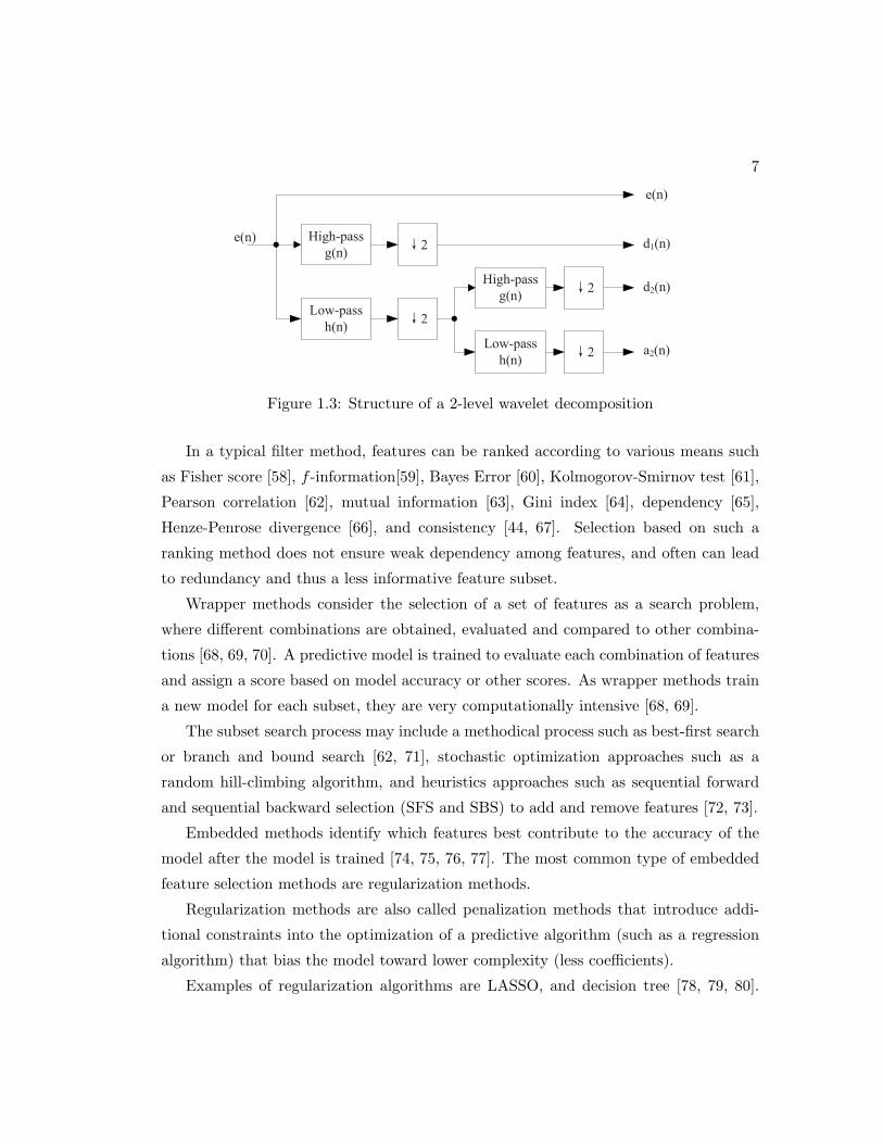
Discrete wavelet decomposition
The purpose of wavelet decomposition is to decompose the original signal into three dis-
joint sub-bands [56]. Discrete wavelet transform (DWT) decomposes discrete sequences
into discrete wavelets coefficients. The structure of a 2-level wavelet decomposition tree
is shown in Fig. 1.3. The input signal is first passed through a low-pass (LPF) and
a high-pass (HPF) filter. Then each filter is followed by a down-sampler with factor
of 2. At the next level, the approximation coefficients are further decomposed into
approximate and detail coefficients.
1.2.2 Prior Works on Feature Selection
Feature selection techniques, in general, can be organized into three categories: filter
methods, wrapper methods and embedded methods.
Filter feature selection methods apply a statistical measure to assign a score to each
feature. The features are ranked by the score and then selected to be either kept or
removed from the feature set. These methods are often univariate and consider each
feature independently [38, 57].
7
1
2
2
Low-pass
h(n)
e(n) High-pass
g(n)
2
a (n)Low-pass
h(n)
High-pass
g(n)
2
2
2 d (n)
d (n)
e(n)
Figure 1.3: Structure of a 2-level wavelet decomposition
In a typical filter method, features can be ranked according to various means such
as Fisher score [58], f -information[59], Bayes Error [60], Kolmogorov-Smirnov test [61],
Pearson correlation [62], mutual information [63], Gini index [64], dependency [65],
Henze-Penrose divergence [66], and consistency [44, 67]. Selection based on such a
ranking method does not ensure weak dependency among features, and often can lead
to redundancy and thus a less informative feature subset.
Wrapper methods consider the selection of a set of features as a search problem,
where different combinations are obtained, evaluated and compared to other combina-
tions [68, 69, 70]. A predictive model is trained to evaluate each combination of features
and assign a score based on model accuracy or other scores. As wrapper methods train
a new model for each subset, they are very computationally intensive [68, 69].
The subset search process may include a methodical process such as best-first search
or branch and bound search [62, 71], stochastic optimization approaches such as a
random hill-climbing algorithm, and heuristics approaches such as sequential forward
and sequential backward selection (SFS and SBS) to add and remove features [72, 73].
Embedded methods identify which features best contribute to the accuracy of the
model after the model is trained [74, 75, 76, 77]. The most common type of embedded
feature selection methods are regularization methods.
Regularization methods are also called penalization methods that introduce addi-
tional constraints into the optimization of a predictive algorithm (such as a regression
algorithm) that bias the model toward lower complexity (less coefficients).
Examples of regularization algorithms are LASSO, and decision tree [78, 79, 80].

8
For example, features can be selected using a tree classifier and a model can then be
trained on the selected features [29, 81]. In LASSO, a penalty term is added to the mean
squared error to reduce the number features selected while minimizing the regression
error. The drawbacks of such a method are its computational cost and sensitivity to
overfitting.
Approaches of information-theoretic feature selection in machine learning have ad-
vanced a lot over the past 15-20 years. Well-known criteria for feature selection include
(1) Mutual Information Based Feature Selection (MIFS) [82], (2) Maximum-Relevance
Minimum-Redundancy (mRMR) [83], (3) Joint Mutual Information (JMI) [84], (4)
MIFS-U [85], (5) Conditional Infomax Feature Extraction (CIFE) [86], (6) Conditional
Mutual Information Maximization (CMIM) [87], and (7) Informative Fragments (IF)
[88].
The study in [89] illustrates that the less complex criteria manage to resist over-
fitting. Among all these criteria, mRMR achieves the lowest leave-one-out test error.
The mRMR makes use of mutual information to select features [83]. The aim is to
penalize a feature’s relevancy by its redundancy based on the presence of the other se-
lected features. The mRMR algorithm is an approximation of the theoretically-optimal
maximum-dependency feature selection algorithm that maximizes the mutual informa-
tion between the joint distribution of the selected features and the classification vari-
able [90]. In general, this algorithm is more efficient than the theoretically-optimal
max-dependency selection and produces a feature set with small pairwise redundancy.
Feature Selection by Regression Tree
Classification and Regression Trees (CART) is one of the predictive modeling approaches
and represents a flexible method that can unveil nonlinear relationships [80]. The tree
creation approach has been proposed in [80] and can be described as follows:
1) Examine all possible binary splits on all features.
2) Select a split with least squared error.
3) Impose the split.
4) Repeat recursively for the two child nodes until a stopping rule is satisfied.

9
mRMR Feature Selection Algorithm
The mutual information between two random variables X taking particular values of x
and Y taking particular values of y is defined as follows:
I(X;Y ) = H(X)−H(X|Y )
where
H(X) = −∑x
P (X = x) logP (X = x)
and
H(X|Y ) =∑y
P (Y = y)H(X|Y = y)
Using the notations and symbols in [83], the goal of max relevance feature selec-
tion scheme is to find a feature set Sm with m features {xi, i = 1, 2, ...,m} such that
these features jointly have the largest relevance with class label c. Mathematically, the
objective is to find the m features such that the following criterion is maximized:
maxxi∈X
D(S, c) =1
m
m∑i=1
I(xi; c)
where X represents the whole feature set containing all features. To avoid redundant
features, the minimum redundancy criterion is added. Mathematically, it finds the m
features such that the following criterion is minimized:
minR(S) =1
m2
∑i
∑j
I(xi;xj)
The mRMR algorithm combines the two criteria and can be described as selecting m
features such that D−R is maximized. The mRMR selection method uses an iterative
algorithm such that in each step the following is maximized:
maxxj∈X−Sm−1
[I(xj ; c)−1
m− 1
∑i
I(xi;xj)]

10
1.2.3 Classifiers
Naive Bayes
Naive Bayes is a classification algorithm that applies the Bayes theorem with the as-
sumption that the predictors are conditionally independent given the class [91]. Given a
feature observation, it assigns to this feature observation a probability of P (cl|X1, ..., Xm)
for each of the l-th class. One common rule is the maximum a posteriori or MAP de-
cision rule which predicts this feature vector as class k whose posterior probability
P (Cl|X1, ..., Xm) achieves the maximum value.
LDA
LDA is one of the most popular linear classifiers that learns a linear classification bound-
ary in the input feature space [92].
SVM
Recently, among all linear classifiers, Support Vector Machine (SVM) has attracted
significant attention. Detailed descriptions of cost-sensitive linear SVM (c-LSVM) can
be found in [5]. Generally speaking, the SVM seeks to find the solution to the following
optimization problem:
min J(w, w0, ξ) =1
2∥w∥2 + C+
N∑i∈C1
ξi + C−N∑
j∈C2
ξj (1.7)
subject to yi(wTxi + w0) ≥ 1− ξi, i = 1, 2, ..., N (1.8)
ξi ≥ 0, i = 1, 2, ..., N (1.9)
where xi represents the r-dimensional feature vector, N represents the total number
of feature vectors used for training the classifier, w represents the orientation of the
discriminating hyperplane and w0 represents the offset of the plane from the origin, yi
represents the class indicator (yi = +1 if xi is from class 1, otherwise yi = −1), ξi
represents the slack variable, and C+, C− represent the misclassification costs for two

11
classes, respectively. After training, the decision function of a linear SVM is given by:
f(x) = sign(
N∑i=1
αiyixTi x+ b) (1.10)
where x represents a new feature vector. The above equation can be simplified as
follows:
f(x) = sign(wTx+ b) (1.11)
where w =∑
i αiyixi. The penalty parameter C+ and C− are usually determined by
the cross-validation step [6]. Leave-one-out cross-validation strategy, which refers to
leaving feature vectors corresponding to a randomly selected seizure out of the training
set, is widely used to avoid overfitting of the model. After the test data are classified, the
hyperplane decision function is smoothed by a moving-average filter in a postprocessing
step in the proposed algorithm.
kernel SVM
Detailed descriptions of kernel SVM can be found in [5]. The decision variable of the
kernel SVM classifier is given by
f(x) =
N∑i=1
αiyiK(xi,x) + b (1.12)
where x represents a testing feature vector, xi represent the feature vectors, αi represent
the Lagrangian coefficients, N represents the total number of feature vectors used for
training the classifier, yi represents the class indicator (yi = +1 if xi is from class 1,
otherwise yi = −1). The parameters αi and b are computed during the training process.
K represents the kernel function. As CART unveils nonlinear relationships, polynomial
SVM with degree of 2 and radial basis function kernel SVM (RBF-SVM) are used and
their performance characteristics are compared.
ADABOOST
Boosting, formulated by Freund and Schapire [93], has been very successful in feature
classification and seizure prediction [94]. Its advantages include adaptivity and strong

12
resistance to overfitting. Given a set of training data, {(x1, y1), (x2, y2), ..., (xN , yN )},where xi belongs to a d-dimensional space X and yi is in the label set {−1. + 1},and given the weak classifiers, the algorithm calls the weak learning algorithm T times
(iterations) for constructing a strong classifier as a linear combination of them:
H(x) = sign(
T∑1
αtht(x)) (1.13)
where ht(x) is the weak or base classifiers generated during the t-th iteration and H(x)
is the final strong classifier. In our algorithm, the base classifier is defined as a decision
stump:
f(x) =
1, x < v
−1, x ≥ v(1.14)
where v is the threshold.
AdaBoost is adaptive as each new weak classifier is built in favor of the misclassified
samples. In each iteration, AdaBoost generates a new weak classifier and updates the
distribution weights representing the importance of the feature samples. The weights
of the misclassified samples are increased, so the new weak classifier focuses more on
samples that previous classifiers have missed.
Neural Network
In machine learning, artificial neural networks (ANNs) represent a family of classifier
models. The feedforward neural network uses the following decision function:
f(x) =
T∑i=1
wih(xTvi) + w0 (1.15)
where h(t) represents a logistic sigmoid function and T represents the number of hidden
neurons.
1.3 Dissertation topics and structure
In this section, we discuss the main topics and the structure of the dissertation.
13
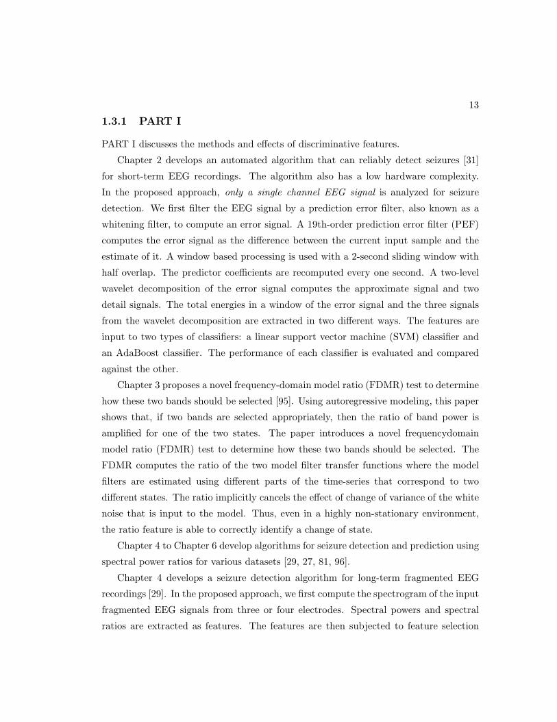
1.3.1 PART I
PART I discusses the methods and effects of discriminative features.
Chapter 2 develops an automated algorithm that can reliably detect seizures [31]
for short-term EEG recordings. The algorithm also has a low hardware complexity.
In the proposed approach, only a single channel EEG signal is analyzed for seizure
detection. We first filter the EEG signal by a prediction error filter, also known as a
whitening filter, to compute an error signal. A 19th-order prediction error filter (PEF)
computes the error signal as the difference between the current input sample and the
estimate of it. A window based processing is used with a 2-second sliding window with
half overlap. The predictor coefficients are recomputed every one second. A two-level
wavelet decomposition of the error signal computes the approximate signal and two
detail signals. The total energies in a window of the error signal and the three signals
from the wavelet decomposition are extracted in two different ways. The features are
input to two types of classifiers: a linear support vector machine (SVM) classifier and
an AdaBoost classifier. The performance of each classifier is evaluated and compared
against the other.
Chapter 3 proposes a novel frequency-domain model ratio (FDMR) test to determine
how these two bands should be selected [95]. Using autoregressive modeling, this paper
shows that, if two bands are selected appropriately, then the ratio of band power is
amplified for one of the two states. The paper introduces a novel frequencydomain
model ratio (FDMR) test to determine how these two bands should be selected. The
FDMR computes the ratio of the two model filter transfer functions where the model
filters are estimated using different parts of the time-series that correspond to two
different states. The ratio implicitly cancels the effect of change of variance of the white
noise that is input to the model. Thus, even in a highly non-stationary environment,
the ratio feature is able to correctly identify a change of state.
Chapter 4 to Chapter 6 develop algorithms for seizure detection and prediction using
spectral power ratios for various datasets [29, 27, 81, 96].
Chapter 4 develops a seizure detection algorithm for long-term fragmented EEG
recordings [29]. In the proposed approach, we first compute the spectrogram of the input
fragmented EEG signals from three or four electrodes. Spectral powers and spectral
ratios are extracted as features. The features are then subjected to feature selection

14
using classification and regression tree (CART). The selected features are then subjected
to a polynomial support vector machine (SVM) classifier with degree of 2. Since all these
features can be extracted by performing the fast Fourier transform (FFT) on the signals
and the classifier requires low hardware complexity [97], the proposed algorithm can be
implemented by the hardware with low complexity and low power consumption.
Chapter 5 develops a patient-specific algorithm that can reliably predict seizures
using either one or two electrodes [27] for short-term dataset. The proposed algorithm
achieves an overall sensitivity higher than 90% and a false positive (FP) rate less than
0.125 FP/hour. The algorithm also requires a low hardware complexity in extracting
features and classification. In the proposed approach, we first compute the spectrogram
of the input EEG signals from one or two electrodes. A window based PSD computation
is used with a 4-second sliding window with half overlap. Thus, the effective window
period is 2 second. Spectral powers and spectral ratios are extracted as features and are
input to a classifier. A postprocessing step is used to remove undesired fluctuations of
the decision output of the classifier. The feature signals are then subjected to feature
selection and classification where two strategies are used. One is the single feature selec-
tion and the other is the multi-dimensional feature selection. While a seizure prediction
system using a single feature requires low hardware complexity and power consumption,
systems using multi-dimensional features achieve a higher prediction reliability. Multi-
dimensional features are selected for patients where systems using a single feature can
not achieve a predetermined requirement.
Chapter 6 develops a patient-specific algorithm that can reliably predict seizures
with high area under curve (AUC) for long-term fragmented EEG recordings [81, 96].
The proposed algorithm compares the performance of different feature sets and different
classifiers for different canine or human subject. In the proposed approach, we first
extract two sets of features. A window based feature extraction is used, where the
window size is 4 second for spectral feature set and is 10 second for the correlation
feature set, respectively. The 10-second window for correlation is chosen for an accurate
estimate of the correlation coefficient. The first feature set includes spectral powers
and spectral ratios. The second feature set includes correlation coefficients between all
possible pairs of electrodes. The two feature sets are then subjected to feature selection
and classification independently. Three classifiers are used and tested on the selected

15
features, which include AdaBoost, radial basis function kernel support vector machine
(RBF-SVM), and artificial neural netwroks (ANN).
1.3.2 PART II
PART II discusses feature selection methods for binary classification and multicalss
classification.
Chapter 7 proposes a new feature selection algorithm based on minimum uncertainty
and sample elimination (referred as MUSE) [98]. The three-step algorithm first quan-
tizes features into bins, ranks the features based on an uncertainty score, selects the
feature with the lowest uncertainty score, and then discards samples based on an im-
purity metric. The discarded samples are not used for selection of subsequent features.
The process is repeated until a stopping criterion is satisfied.
Chapter 8 proposes a new multi-class feature selection criterion based on minimum
uncertainty (referred as M3U) [99]. In this chapter, we propose a three-step algorithm
that first quantizes features into bins, computes an uncertainty vector for each feature
and all sample in each feature, and finally iteratively selects features that achieves the
minimum mean minimum uncertainty (M3U). The proposed iterative feature selection
algorithm includes two minimization steps and one expectation step, which include (1)
find the minimum uncertainty (MU) score for each feature sample given a feature subset,
(2) compute the mean minimum uncertainty score (M2U) for the feature subset, and (3)
select the feature that achieves the minimum mean minimum uncertainty score (M3U).
1.4 Contributions of the dissertation
In this section, main contribution of each part is discussed.
First, Part I introduces a novel frequency-domain model ratio (FDMR) test to
identify the discriminative ratio features from a single-channel signal. Although the
ratios in [30, 27] were chosen using band definitions from neuroscience, such as δ, θ, α,
β, and γ, and ranking algorithms from machine learning, the actual bands do not need
to coincide with these bands. Several theoretical questions remain unanswered. Why
the ratio features amplify the discrimination remains unexplained. How the two bands
should be chosen to maximize the discrimination remains unknown. These questions

16
are answered in this Chapter 3. Using an auto-regressive model, we argue that a state
change in a time-series corresponds to a change in the filter model. From the ratio
of the frequency-domain characteristics of these two models, i.e., one frequency-domain
response normalized with respect to the other, we can determine two bands such that for
one band the ratio is much higher than 1 and for the other much less than 1. We show
that the ratio of spectral powers of a single time-series in these two bands is amplified
for one of the two states. This chapter shows that the effect of the non-stationarity
of the noise power can be eliminated by using the ratio of spectral powers when the
signal-to-noise ratio (SNR) is high. This chapter also shows that, even when the SNR
is low, the ratio of spectral power ratios can significantly discriminate the state of the
time-series if a postprocessing step such as a second-order Kalman filter is applied to
the ratio feature. Thus, ratio of spectral powers can be used for identifying state of a
non-stationary time-series assuming the model filters for the two states are different.
Second, Part I shows that combining the PSD features such as absolute spectral
powers, relative spectral powers and spectral power ratios as a feature set and then
carefully selecting a small number features from a few electrodes can achieve a good de-
tection and prediction performances on short-term datasets and long-term fragmented
datasets. Since only a few features from a few electrodes are carefully selected us-
ing various feature selection method, the proposed algorithms also have a low-power
and low-complexity hardware design. In low-power and low-complexity hardware de-
sign, the first key consideration is the number of sensors used to collect EEG signals.
Electrode selection is an essential step before feature selection as sensors and analog-to-
digital converters (A/D) can be highly power consuming for an implantable or wearable
biomedical device. The second key consideration is selecting useful features that are
computationally simple and are indicative of upcoming seizure activities. The third key
consideration is the choice of classifier. Based on the selection of the classifier, a criteria
for electrode and feature selection should be chosen accordingly in order to achieve the
best classification performance.
Part II proposes novel feature selection methods for binary classification (MUSE)
and multi-class classification (M3U). The main contribution of MUSE is that a new
feature selection algorithm based on minimum uncertainty and sample elimination (re-
ferred as MUSE) is proposed. The sample elimination process reduces redundancy and
17
the selection of a feature with the least uncertainty score increases relevance. The dis-
carding of the samples and the selection of the feature are both nonlinear operations
and are ideal for general machine learning applications where feature samples may not
necessarily be linearly separable. The main contribution of M3U is a new multi-class
feature selection criterion based on minimum uncertainty. To the best of our knowledge,
the one-versus-all (OVA) uncertainty vector is defined in M3U is is a new sample-wise
criterion that has not been proposed before. Given a feature sample in a particular
feature, this uncertainty score illustrates how good the bin (corresponding to the fea-
ture sample) is to separate the class (corresponding to the feature sample) from the
remaining classes.

Part I
Feature Identification, Extraction
and Classification
18
Chapter 2
Seizure Detection from
Short-Term EEG Recordings
using Wavelet Decomposition of
the Prediction Error Signal
Our main objective is to develop an automated algorithm that can reliably detect
seizures. The algorithm should also have a low hardware complexity. In the proposed
approach [31], only a single channel EEG signal is analyzed for seizure detection. We
first filter the EEG signal by a prediction error filter, also known as a whitening filter,
to compute an error signal. A 19th-order prediction error filter (PEF) computes the
error signal as the difference between the current input sample and the estimate of it. A
window based processing is used with a 2-second sliding window with half overlap. The
predictor coefficients are recomputed every one second. A two-level wavelet decompo-
sition of the error signal computes the approximate signal and two detail signals. The
total energies in a window of the error signal and the three signals from the wavelet de-
composition are extracted in two different ways. The features are input to two types of
classifiers: a linear support vector machine (SVM) classifier and an AdaBoost classifier.
The performance of each classifier is evaluated and compared against the other.
19
20
2.1 Materials and Methods
2.1.1 Patients Database
We have trained and tested our algorithm on the Freiburg EEG database [100], which
is available to any lab by request. According to [100], this database contains electrocor-
ticogram (ECoG) or iEEG from 21 patients with medically intractable focal epilepsy.
We have chosen 18 of the available datasets of 21 patients, who have three or more
seizures (the minimum number for cross-validation). Each 2-s-long window of iEEG
has been categorized as ictal (containing a seizure), interictal (at least 1 h preceding or
postceding a seizure), preictal (in 60 min preceding a seizure onset), or artifact. Half
an hour of iEEG recordings preceding preictal and an hour of those postceding seizure
offset are excluded in training. The Freiburg database contains six of iEEG recordings
from grid, strip, or depth-electrodes, three near the seizure focus (focal) and the oth-
er three distal to the focus (afocal). Seizure onset times and artifacts were identified
by certified epileptologists. The data were collected at 256 Hz (Patient 12 at 512 Hz)
sampling rate with 16 bit analog-to-digital converters.
2.1.2 System Architecture
Classifier
Prediction
Error
Filter
w(n)
Wavelet
Decomposition
EEG
signal
s(n)
Error
Signal
e(n)
+1
0
Feture
Vectors
Feature
Extractor
e(n),or Wavelet
Coefficients
a(n) or di(n)
Esitimate
Prediction
Error
Filter
Coeffcients
w(n)
Figure 2.1: System architecture for seizure detection
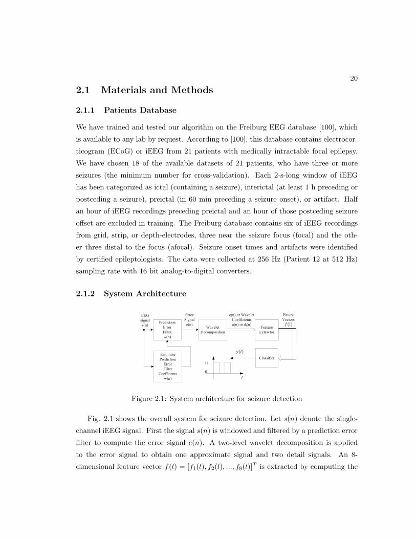
Fig. 2.1 shows the overall system for seizure detection. Let s(n) denote the single-
channel iEEG signal. First the signal s(n) is windowed and filtered by a prediction error
filter to compute the error signal e(n). A two-level wavelet decomposition is applied
to the error signal to obtain one approximate signal and two detail signals. An 8-
dimensional feature vector f(l) = [f1(l), f2(l), ..., f8(l)]T is extracted by computing the

21
total power for the error signal and the three signals obtained by wavelet decomposition
inside the sliding window. The feature vectors are then subjected to training and
classification. The output of the system y(l) represents the detection signal. Two types
of classifiers are considered. These include: the linear SVM and the AdaBoost. The
training follows leave-one-out procedure, where the seizure to be tested is not used for
training.
2.1.3 Feature Extraction
This section describes the method for feature extraction, which includes prediction error
filter, a 2-level wavelet decomposition and power computation.
Window-based signal processing
The input signal is divided into the input segments (or windows) and the signal is
processed segment by segment. Each segment has a 50% overlap with its neighbour
segment.
Preprocessing
In the first step, EEG data is preprocessed to remove its mean. The demeaned signal is
then filtered by a PEF to remove the predictable component of the EEG signal. Each
window is 2 seconds long and has 50% overlap. The PEF is then used to compute the
error signal for next one second. Thus, effective feature computation rate is one per
second.
Let wf represent tap-weights vector of an m-tap predictor (or a mth-order PEF).
Coefficients of the PEF can be computed by solving the Wiener-Hopf equation: wf =
R−1r, where R represents the autocorrelation matrix of the input sample vector of a
window, and r represents the cross-correlation vector between the input sample vector
and its delayed versions. Levinson-Durbin algorithm is used to solve the above equation
[101].
A 19th-order PEF is chosen for this dataset. A singular value decomposition of
the covariance matrix is performed for patient No. 1 to find the optimal order of the
predictor. Fig. 2.2(a) and Fig. 2.2(b) show the plots of the percentage of total energy

22
captured by the predictor versus the predictor’s order using (a) an hour’s inter-ictal
data from patient No. 1 while the patient is awake and (b) an hour’s inter-ictal data
from patient No. 1 while the patient is sleeping, respectively. A 19-tap predictor
(equivalently, 19th order or 20-tap PEF) can capture about 95% of the total energy of
the signal.
0 10 20 30 4020
30
40
50
60
70
80
90
100
No. of SV
Tot
al e
nerg
y (%
)
awake
0 10 20 30 4020
30
40
50
60
70
80
90
100
No. of SV
Tot
al e
nerg
y (%
)
sleep
Figure 2.2: Percentage of total energy captured by the predictor versus the predictor’sorder using (a) an hour’s inter-ictal data from patient No. 1 while the patient is awakeand (b) an hour’s inter-ictal data from patient No. 1 while the patient is sleeping.
Figure 2.3: Spectrograms of the EEG signal (left) and its error signal (right) usinginterictal recordings for the 16th hour from patient No. 1.
Fig. 2.3 shows the spectrograms of the EEG signal and its error signal corresponding
to the interictal recordings for patient No. 1 in the 16th hour, where undesired harmonics
in the interictal period are filtered and the dominance of the low frequencies on the total
power is eliminated after prediction error filtering.

23
Discrete wavelet decomposition
A two-level wavelet decomposition is applied to the error signal to compute wavelet
coefficients at different levels.
Feature extractor
Two types of features are extracted from the error signal and the wavelet coefficients:
one is the total power and the other is the sum of the logarithm of the absolute feature
values (also equivalently, logarithm of the product of the absolute feature values). Total
power for each segment is obtained by computing the sum of the squared value of the
wavelet coefficients (or the error signal). Mathematically, these are computed as:
f ′(l) =∑n∈Il
log|e(n)| (2.1)
f ′′(l) =∑n∈Il
e2(n) (2.2)
where Il = {(l − 1)fs + 1, ..., lfs} represents the samples of the l-th window. Fig. 2.4
shows the block diagram of feature extraction, where a total number of 8 features (f1(l)
to f8(l)) are extracted from the error signal, e(n), and the wavelet coefficients, a2(n),
d2(n), and d1(n); four of these features represent the mean power and the remaining
four represent the logarithm of the product of the absolute values. For the AdaBoost
classifier, all 8 features are input to the classifier. The classifier always selects between
1 to 4 out of the 8 features.
d1(n)a2(n) d2(n)e(n)
Accumu-
lator
Accumu-
lator
Accumu-
lator
Accumu-
latorAccumu-
lator
Accumu-
lator
Accumu-
lator
Accumu-
lator
f1(l) f2(l) f3(l) f4(l) f5(l) f6(l) f7(l) f8(l)
Figure 2.4: Feature extraction.
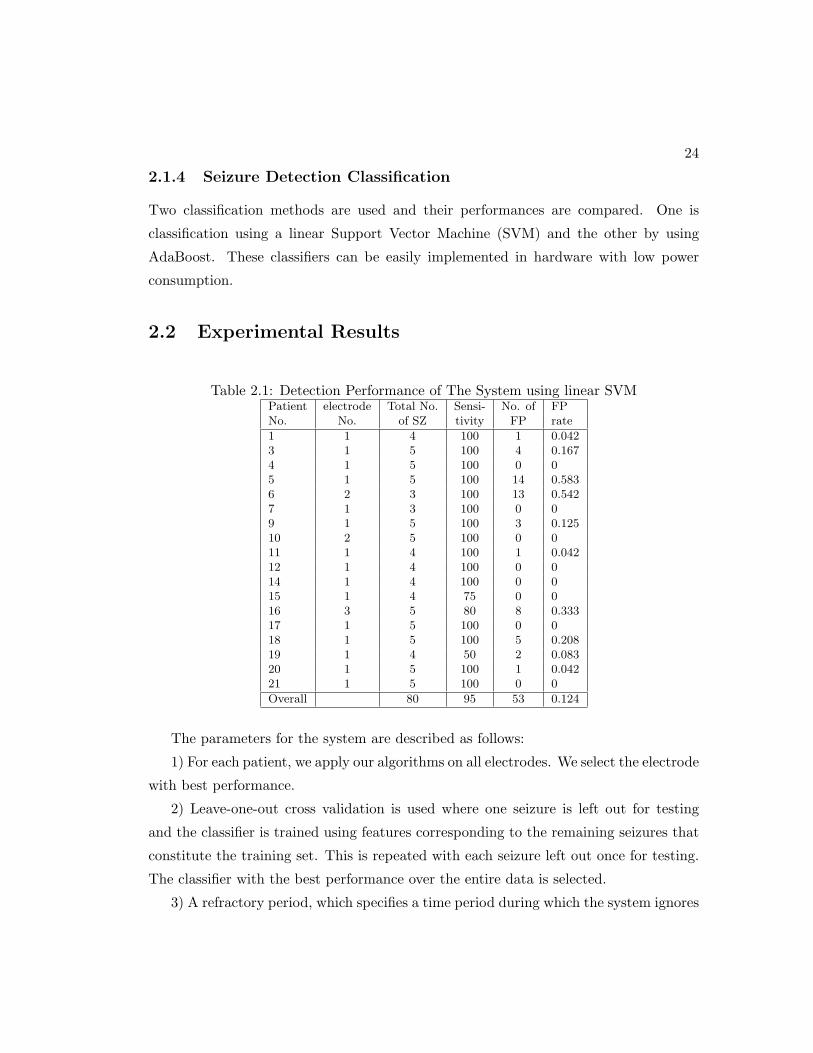
24
2.1.4 Seizure Detection Classification
Two classification methods are used and their performances are compared. One is
classification using a linear Support Vector Machine (SVM) and the other by using
AdaBoost. These classifiers can be easily implemented in hardware with low power
consumption.
2.2 Experimental Results
Table 2.1: Detection Performance of The System using linear SVMPatient electrode Total No. Sensi- No. of FPNo. No. of SZ tivity FP rate
1 1 4 100 1 0.0423 1 5 100 4 0.1674 1 5 100 0 05 1 5 100 14 0.5836 2 3 100 13 0.5427 1 3 100 0 09 1 5 100 3 0.12510 2 5 100 0 011 1 4 100 1 0.04212 1 4 100 0 014 1 4 100 0 015 1 4 75 0 016 3 5 80 8 0.33317 1 5 100 0 018 1 5 100 5 0.20819 1 4 50 2 0.08320 1 5 100 1 0.04221 1 5 100 0 0
Overall 80 95 53 0.124
The parameters for the system are described as follows:
1) For each patient, we apply our algorithms on all electrodes. We select the electrode
with best performance.
2) Leave-one-out cross validation is used where one seizure is left out for testing
and the classifier is trained using features corresponding to the remaining seizures that
constitute the training set. This is repeated with each seizure left out once for testing.
The classifier with the best performance over the entire data is selected.
3) A refractory period, which specifies a time period during which the system ignores

25
Table 2.2: Detection Performance of The System using AdaboostPatient electrode Total No. Sensi- No. of FPNo. No. of SZ tivity FP rate
1 1 4 100 0 03 1 5 100 0 04 2 5 100 0 05 2 5 100 5 0.2086 2 3 100 7 0.2927 1 3 100 0 09 1 5 100 3 0.12510 2 5 100 0 011 1 4 100 0 012 1 4 100 0 014 3 4 100 1 0.04215 3 4 75 0 016 2 5 100 8 0.33317 1 5 100 0 018 1 5 100 7 0.29219 1 4 100 1 0.04220 5 5 100 0 021 3 5 100 0 0
Overall 80 98.75 32 0.075∗ Features for patient No. 19 are computed as the time difference of the original features.
all the subsequent triggers once it’s triggered, is introduced. The refractory period is
set to be 10 minutes.
Test Results using linear SVM classifier are shown in Table 2.1. Only the first 4
features {f1(n), .., f4(n)} are used in the training phase. The average sensitivity is 95%
and the average FP rate is 0.124 FP per hour.
Test Results using AdaBoost and all 8 features are shown in Table 2.2. The perfor-
mance is improved as the sensitivity is increased to 98.75% and the FP rate reduces to
0.075 FP per hour. For patient No. 19, in order to detect all seizures, a new feature
was derived by taking the difference of the log features at certain time and at 30s prior
to that time point.
2.3 Discussion
Many approaches have been presented for detecting seizures in epileptic patients. A
seizure detection algorithm that utilizes 3 focus channels was proposed in [102]. In
[103], this proposed algorithm was tested on the Freiburg database [100] and achieved
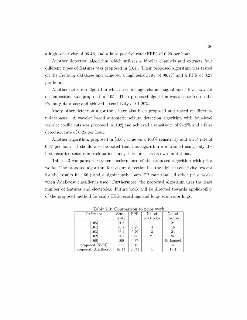
26
a high sensitivity of 96.4% and a false positive rate (FPR) of 0.20 per hour.
Another detection algorithm which utilizes 4 bipolar channels and extracts four
different types of features was proposed in [104]. Their proposed algorithm was tested
on the Freiburg database and achieved a high sensitivity of 98.7% and a FPR of 0.27
per hour.
Another detection algorithm which uses a single channel signal and 5-level wavelet
decomposition was proposed in [105]. Their proposed algorithm was also tested on the
Freiburg database and achived a sensitivity of 91.29%.
Many other detection algorithms have also been proposed and tested on differen-
t databases. A wavelet based automatic seizure detection algorithm with four-level
wavelet coefficients was proposed in [102] and achieved a sensitivity of 94.2% and a false
detection rate of 0.25 per hour.
Another algorithm, proposed in [106], achieves a 100% sensitivity and a FP rate of
0.37 per hour. It should also be noted that this algorithm was trained using only the
first recorded seizure in each patient and, therefore, has its own limitations.
Table 2.3 compares the system performance of the proposed algorithm with prior
works. The proposed algorithm for seizure detection has the highest sensitivity (except
for the results in [106]) and a significantly lower FP rate than all other prior works
when AdaBoost classifier is used. Furthermore, the proposed algorithm uses the least
number of features and electrodes. Future work will be directed towards applicability
of the proposed method for scalp EEG recordings and long-term recordings.
Table 2.3: Comparison to prior workReference Sensi- FPR No. of No. of
tivity electrodes features
[105] 91.3 - 1 24[104] 98.7 0.27 4 16[103] 96.4 0.20 3 24[102] 94.2 0.25 21 84[106] 100 0.37 - 6/channel
proposed (SVM) 95.0 0.12 1 4proposed (AdaBoost) 98.75 0.075 1 1∼4
Chapter 3
FDMR: Frequency-Domain
Model Ratio for Identifying
Change of State from a Single
Time-Series
Although the ratios in [30, 27] were chosen using band definitions from neuroscience,
such as δ, θ, α, β, and γ, and ranking algorithms from machine learning, the actual
bands do not need to coincide with these bands. Several theoretical questions remain
unanswered. Why the ratio features amplify the discrimination remains unexplained.
How the two bands should be chosen to maximize the discrimination remains unknown.
These questions are answered in this chapter [95]. Using an auto-regressive model, we
argue that a state change in a time-series corresponds to a change in the filter model.
From the ratio of the frequency-domain characteristics of these two models, i.e., one
frequency-domain response normalized with respect to the other, we can determine two
bands such that for one band the ratio is much higher than 1 and for the other much
less than 1. We show that the ratio of spectral powers of a single time-series in these
two bands is amplified for one of the two states. This chapter shows that the impact of
the non-stationarity of the noise power can be eliminated by using the ratio of spectral
powers when the signal-to-noise ratio (SNR) is high. This paper also shows that, even
27

28
when the SNR is low, the ratio of spectral power ratios can significantly discriminate
the state of the time-series if a postprocessing step such as a second-order Kalman filter
is applied to the ratio feature. Thus, ratio of spectral powers can be used for identifying
state of a non-stationary time-series assuming the model filters for the two states are
different.
3.1 Ratio of Spectral Powers of Two Different Bands
Consider a discrete-time system described by an auto-regressive model as shown in Fig.
3.1. This system changes from one state to a second state. Our goal is to identify
the two states from the time-series. Note that the same time-series corresponds to two
different states at different time instances. We first make the following assumptions:
(1) Assume the system is driven by a white noise w1(n) with zero mean and variance
σ2w1
at State 1, and is driven by a white noise w2(n) with zero mean and variance σ2w2
at State 2.
(2) Assume the system has an impulse response of h1(n) at State 1 and an impulse re-
sponse of h2(n) at State 2. The frequency responses of h1(n) and h2(n) are represented
by H1(ejω) and H2(e
jω), respectively.
(3) Assume the signals s1(n) and s2(n) correspond to the outputs of H1 and H2, re-
spectively.
(4) The measured signals are x1(n) and x2(n). s1(n) and s2(n) are never measured.
(5) Assume x1(n) and x2(n) are obtained by adding a white gaussian noise v1(n) (with
zero mean and variance σ2v1) to s1(n) and by adding a white gaussian noise v2(n) (with
zero mean and variance σ2v2) to s2(n), respectively. x1(n) and x2(n) correspond to the
measured time-series from a single sensor at two different states.
Identifying the two states of the system is, therefore, equivalent to identifying and
extracting discriminative features from the outputs of the system.
To illustrate how the ratio of two spectral powers cancels the effect of the change
of variance at the input of the auto-regressive model, we consider an example. Suppose
the magnitudes of frequency responses for the system with two states are shown in Fig.
3.2, where the system in both states is a low-pass filter. However, note that H1 is an
ideal low-pass filter with a constant pass-band gain while H2 is not. The frequency

29
White noise
1(!) "1
#1(!)
$1(!) %1(!)
(a)
White noise
2(!) "2 #2(!)
$2(!) %2(!)
(b)
Figure 3.1: System models at (a) State 1 and (b) State 2.
response of the system in State 2, referred as H2, has twice the magnitude of H1 in the
frequency band of [0, 0.2π]; and the magnitude of H2 is only half of H1 in the frequency
band of [0.3π, 0.4π].
ω (in π)0 0.2 0.4 0.6 0.8 1
mag
nitu
de
0
0.5
1
1.5
2
2.5
H1
H2
Figure 3.2: magnitudes of frequency responses for the system in two states.
3.1.1 Stationary case
First, we assume a stationary case where the variances of the input noises of the two
states remain the same and are equal to a constant, i.e., σ2w1
= σ2w2
= c1. We also
assume that the variances of the additive white Gaussian noise (AWGN) at the two
states also remain the same and are equal to a constant, i.e., σ2v1 = σ2
v2 = c2 Then the
power spectral density (PSD) of x1(n) and x2(n) can be calculated as follows:
Sx1(ω) = σ2w1|H1(e
jω)|2 + σ2v1 = c1|H1(e
jω)|2 + c2 (3.1)
Sx2(ω) = σ2w2|H2(e
jω)|2 + σ2v2 = c2|H2(e
jω)|2 + c2 (3.2)
(3.3)

30
Since |H2(ejω)| ≈ 2|H1(e
jω)| for w in [0, 0.2π], the band power in [0, 0.2π] can be used
as a discriminative feature to separate the signals s1(n) and s2(n). Mathematically, let
Px1([0, 0.2π]) and Px2([0, 0.2π]) represent the band powers for x1 and x2 in the frequency
band [0, 0.2π], respectively. This band power for x1 and x2 can be computed as follows:
Px1([0, 0.2π]) =
∫ 0.2π
0(c1|H1(e
jω)|2 + c2)dω (3.4)
= Ps1([0, 0.2π]) + 0.2πc2 (3.5)
Px2([0, 0.2π]) =
∫ 0.2π
0(c1|H2(e
jω)|2 + c2)dω (3.6)
= Ps2([0, 0.2π]) + 0.2πc2 (3.7)
=
∫ 0.2π
0(4c1|H1(e
jω)|2 + c2)dω (3.8)
= 4Ps1([0, 0.2π]) + 0.2πc2 (3.9)
Since the band power of s1(n) in the frequency band of [0, 0.2π] is approximately four
times of the band power of s2(n) in the same frequency band, the band power of the
output signal x1(n) in the frequency band of [0, 0.2π, ] is significantly higher than the
band power of the output signal x2(n) in the same frequency band. Theoretically, this
band power is a discriminative feature to separate x1 and x2.
Assume that the outputs, x1 and x2, are both divided into 200 segments and the
two signals are processed segment by segment. Each segment is 10 seconds long and
contains 2560 samples. PSD and band power in the frequency band of [0, 0.2π] are
computed for each segment. Fig. 3.3 illustrates the histogram of the natural logarithm
of the band power in the frequency band of [0, 0.2π] for segments of x1 and x2, where
c1 = 1 and the signal-to-noise-ratio (SNR) is chosen as SNR=σ2s1
σ2v1
=σ2s2
σ2v2
= 20dB. This
corresponds to c2 = 0.0475. As shown in the figure, the mean of the band power in the
frequency band of [0, 0.2π] for State 1 is much lower than that of State 2 and such a
feature is indeed a discriminative feature to separate the two states.
Similarly, since |H2(ejω)| ≈ 0.5|H1(e
jω)| for w in [0.3π, 0.4π], we have the following

31
band power in [0, 0.2π]17 17.5 18 18.5 19
hist
ogra
m
0
20
40
60
80state 1state 2
Figure 3.3: Histogram of the logarithm of the band power in the frequency band of[0, 0.2π] for segments of x1 and x2..
relationship:
Px2([0.3π, 0.4π]) =
∫ 0.4π
0.3π(c1|H2(e
jω)|2 + c2)dω (3.10)
= Ps2([0.3π, 0.4π]) + 0.1πc2 (3.11)
=
∫ 0.4π
0.3π(0.25c1|H1(e
jω)|2 + c2)dω (3.12)
= 0.25Ps1([0.3π, 0.4π]) + 0.1πc2 (3.13)
Thus, the band power in [0.3π, 0.4π] can also be used as a discriminative feature to
separate the signals s1(n) and s2(n).
3.1.2 Non-stationary case
However, the band powers may not be as discriminative as shown in Fig. 3.3 when
the input noise variances change considerably. In many cases, the input noise variance
remains same for a certain period of time and then changes during next period of time.
We still assume that the outputs, x1 and x2, are both divided into 200 segments, and
the two signals are processed segment by segment. Each segment is 10 seconds long
and contains 2560 samples. The input noise variance is fixed for each segment, but
it is different for different segments. This means that the noise variance remains the
same for 10 seconds, and changes to a different value in the next 10 seconds. Therefore,
each segment is stationary, but the entire signal is not. Assume that the input noise
variances for w1(n) and w2(n) for different segments are distributed uniformly between
1 and 16, i.e., σ2w1, σ2
w2∼ U(1, 16). Suppose that the signal to noise ratios (SNR) at
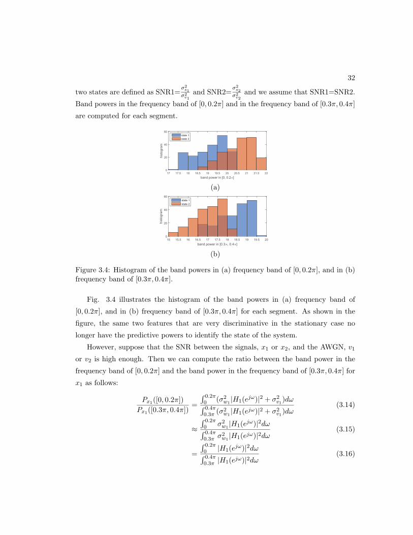
32
two states are defined as SNR1=σ2s1
σ2v1
and SNR2=σ2s2
σ2v2
and we assume that SNR1=SNR2.
Band powers in the frequency band of [0, 0.2π] and in the frequency band of [0.3π, 0.4π]
are computed for each segment.
band power in [0, 0.2 ]
17 17.5 18 18.5 19 19.5 20 20.5 21 21.5 22
his
togra
m
0
20
40
60
state 1
state 2
(a)
band power in [0.3 , 0.4 ]
15 15.5 16 16.5 17 17.5 18 18.5 19 19.5 20
his
togra
m
0
20
40
60
state 1
state 2
(b)
Figure 3.4: Histogram of the band powers in (a) frequency band of [0, 0.2π], and in (b)frequency band of [0.3π, 0.4π].
Fig. 3.4 illustrates the histogram of the band powers in (a) frequency band of
[0, 0.2π], and in (b) frequency band of [0.3π, 0.4π] for each segment. As shown in the
figure, the same two features that are very discriminative in the stationary case no
longer have the predictive powers to identify the state of the system.
However, suppose that the SNR between the signals, x1 or x2, and the AWGN, v1
or v2 is high enough. Then we can compute the ratio between the band power in the
frequency band of [0, 0.2π] and the band power in the frequency band of [0.3π, 0.4π] for
x1 as follows:
Px1([0, 0.2π])
Px1([0.3π, 0.4π])=
∫ 0.2π0 (σ2
w1|H1(e
jω)|2 + σ2v1)dω∫ 0.4π
0.3π (σ2w1|H1(ejω)|2 + σ2
v1)dω(3.14)
≈∫ 0.2π0 σ2
w1|H1(e
jω)|2dω∫ 0.4π0.3π σ2
w1|H1(ejω)|2dω
(3.15)
=
∫ 0.2π0 |H1(e
jω)|2dω∫ 0.4π0.3π |H1(ejω)|2dω
(3.16)

33
Similarly, we can compute the ratio between the band power in the frequency band
of [0, 0.2π] and the band power in the frequency band of [0.3π, 0.4π] for x2 as follows:
Px2([0, 0.2π])
Px2([0.3π, 0.4π])≈∫ 0.2π0 |H2(e
jω)|2dω∫ 0.4π0.3π |H2(ejω)|2dω
(3.17)
Such a spectral power ratio for x2 is significantly higher than x1 for the following reason:
(Px2 ([0,0.2π])
Px2 ([0.3π,0.4π])
)(
Px1 ([0,0.2π])
Px1 ([0.3π,0.4π])
) =
( ∫ 0.2π0 |H2(ejω)|2dω∫ 0.4π0.3π |H2(ejω)|2dω
)( ∫ 0.2π
0 |H1(ejω)|2dω∫ 0.4π0.3π |H1(ejω)|2dω
) (3.18)
=
(∫ 0.2π0 |H2(e
jω)|2dω∫ 0.2π0 |H1(ejω)|2dω
)(∫ 0.4π0.3π |H1(e
jω)|2dω∫ 0.4π0.3π |H2(ejω)|2dω
)(3.19)
≈
(∫ 0.2π0 4|H1(e
jω)|2dω∫ 0.2π0 |H1(ejω)|2dω
)(∫ 0.4π0.3π 4|H2(e
jω)|2dω∫ 0.4π0.3π |H2(ejω)|2dω
)(3.20)
=16 (3.21)
The spectral power ratio between the band power in the frequency band of [0, 0.2π]
and the band power in the frequency band of [0.3π, 0.4π] for x2 is 16 times that of
x1. Equations (3.16) to (3.21) illustrate that the spectral power ratio feature not only
cancels the input noise variance under high SNR assumption, but also amplifies the
differences between the outputs from two states.
Therefore, in general, we propose the following algorithm to identify discriminative
spectral power ratios to identify the system states:
Algorithm 1 Algorithm for identifying discriminative spectral power ratios using trans-fer functions
(1) Plot the filter ratios as RH(ejω) = |H2(ejω)||H1(ejω)|
(2) Identify the frequency band 1 as B1 where RH(ejω) > 1(3) Identify the frequency band 2 as B2 where RH(ejω) < 1(4) Compute the band power in frequency band 1 as Px(B1)(5) Compute the band power in frequency band 2 as Px(B2)(6) Compute the spectral power ratio between the power in B1 and the power in B2
as Rx(B1, B2) = Px(B1)Px(B2)
for each state.

34
Theorem 1. The ratio of Spectral powers obtained from Algorithm 1 amplifies the
discrimination between the two states.
Proof. Suppose Rx1(B1, B2) =Px1 (B1)
Px1 (B2)and Rx2(B1, B2) =
Px2 (B1)
Px2 (B2)represent the spec-
tral power ratios between the power in B1 and the power in B2 for x1 and x2, respec-
tively. We can prove that this ratio feature increases significantly for x2, regardless of
the change of the input noise variances. We first compute the ratio between the band
power in the frequency band of B1 and the band power in the frequency band of B2 for
x1 as follows:
Rx1(B1, B2) =Px1(B1)
Px1(B2)(3.22)
=
∫B1
(σ2w1|H1(e
jω)|2 + σ2v1)dω∫
B2(σ2
w1|H1(ejω)|2 + σ2
v1)dω(3.23)
≈σ2w1
∫B1
|H1(ejω)|2dω
σ2w1
∫B2
|H1(ejω)|2dω(3.24)
=
∫B1
|H1(ejω)|2dω∫
B2|H1(ejω)|2dω
(3.25)
Similarly, this spectral power ratio for x2 can be computed as follows:
Rx2(B1, B2) =
∫B1
|H2(ejω)|2dω∫
B2|H2(ejω)|2dω
(3.26)
By comparing the two spectral power ratios for x1 and x2, we have the following
relationship:
Rx2(B1, B2)
Rx1(B1, B2)=
(Px2 (B1)
Px2 (B2)
)(Px1 (B1)
Px1 (B2)
) (3.27)
=
(∫B1
|H2(ejω)|2dω∫B2
|H2(ejω)|2dω
)(∫
B1|H1(ejω)|2dω∫
B2|H1(ejω)|2dω
) (3.28)
=
(∫B1
|H2(ejω)|2dω∫
B1|H1(ejω)|2dω
)(∫B2
|H1(ejω)|2dω∫
B2|H2(ejω)|2dω
)(3.29)
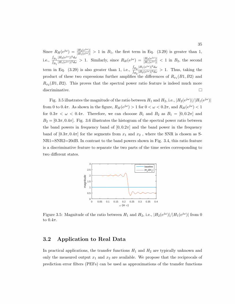
35
Since RH(ejω) = |H2(ejω)||H1(ejω)| > 1 in B1, the first term in Eq. (3.29) is greater than 1,
i.e.,
∫B1
|H2(ejω)|2dω∫B1
|H1(ejω)|2dω> 1. Similarly, since RH(ejω) = |H2(ejω)|
|H1(ejω)| < 1 in B2, the second
term in Eq. (3.29) is also greater than 1, i.e.,
∫B2
|H1(ejω)|2dω∫B2
|H2(ejω)|2dω> 1. Thus, taking the
product of these two expressions further amplifies the differences of Rx1(B1, B2) and
Rx2(B1, B2). This proves that the spectral power ratio feature is indeed much more
discriminative.
Fig. 3.5 illustrates the magnitude of the ratio betweenH1 andH2, i.e., |H2(ejω)|/|H1(e
jω)|from 0 to 0.4π. As shown in the figure, RH(ejω) > 1 for 0 < ω < 0.2π, and RH(ejω) < 1
for 0.3π < ω < 0.4π. Therefore, we can chooose B1 and B2 as B1 = [0, 0.2π] and
B2 = [0.3π, 0.4π]. Fig. 3.6 illustrates the histogram of the spectral power ratio between
the band powers in frequency band of [0, 0.2π] and the band power in the frequency
band of [0.3π, 0.4π] for the segments from x1 and x2 , where the SNR is chosen as S-
NR1=SNR2=20dB. In contrast to the band powers shown in Fig. 3.4, this ratio feature
is a discriminative feature to separate the two parts of the time series corresponding to
two different states.
ω (in π)0 0.05 0.1 0.15 0.2 0.25 0.3 0.35 0.4
mag
nitu
de
0
0.5
1
1.5
2
2.5
3baseline|H
2|/|H
1|
Figure 3.5: Magnitude of the ratio between H1 and H2, i.e., |H2(ejω)|/|H1(e
jω)| from 0to 0.4π.
3.2 Application to Real Data
In practical applications, the transfer functions H1 and H2 are typically unknown and
only the measured output x1 and x2 are available. We propose that the reciprocals of
prediction error filters (PEFs) can be used as approximations of the transfer functions
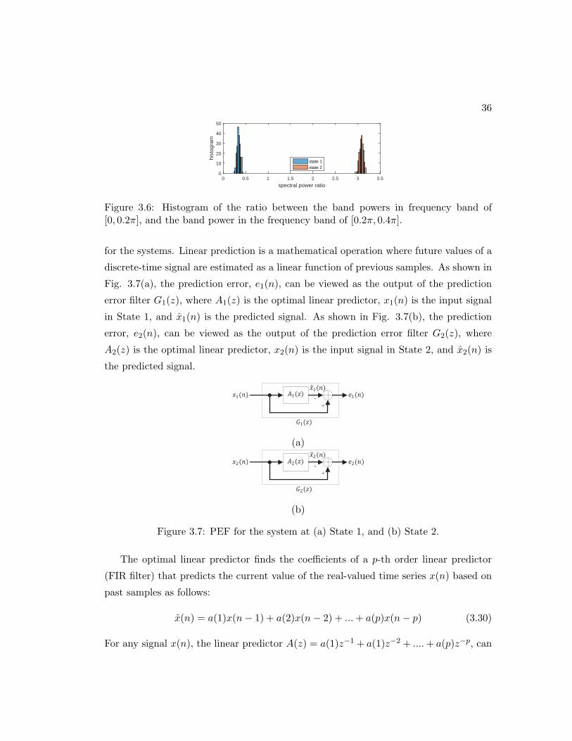
36
spectral power ratio0 0.5 1 1.5 2 2.5 3 3.5
hist
ogra
m
0
10
20
30
40
50
state 1state 2
Figure 3.6: Histogram of the ratio between the band powers in frequency band of[0, 0.2π], and the band power in the frequency band of [0.2π, 0.4π].
for the systems. Linear prediction is a mathematical operation where future values of a
discrete-time signal are estimated as a linear function of previous samples. As shown in
Fig. 3.7(a), the prediction error, e1(n), can be viewed as the output of the prediction
error filter G1(z), where A1(z) is the optimal linear predictor, x1(n) is the input signal
in State 1, and x1(n) is the predicted signal. As shown in Fig. 3.7(b), the prediction
error, e2(n), can be viewed as the output of the prediction error filter G2(z), where
A2(z) is the optimal linear predictor, x2(n) is the input signal in State 2, and x2(n) is
the predicted signal.
1(!) "1(#) -
!1(") #1(")
+
1(!)
(a)
2(!) "2(#) $2(!)
%2(!)
+
2(!)
-
(b)
Figure 3.7: PEF for the system at (a) State 1, and (b) State 2.
The optimal linear predictor finds the coefficients of a p-th order linear predictor
(FIR filter) that predicts the current value of the real-valued time series x(n) based on
past samples as follows:
x(n) = a(1)x(n− 1) + a(2)x(n− 2) + ...+ a(p)x(n− p) (3.30)
For any signal x(n), the linear predictor A(z) = a(1)z−1 + a(1)z−2 + ....+ a(p)z−p, can
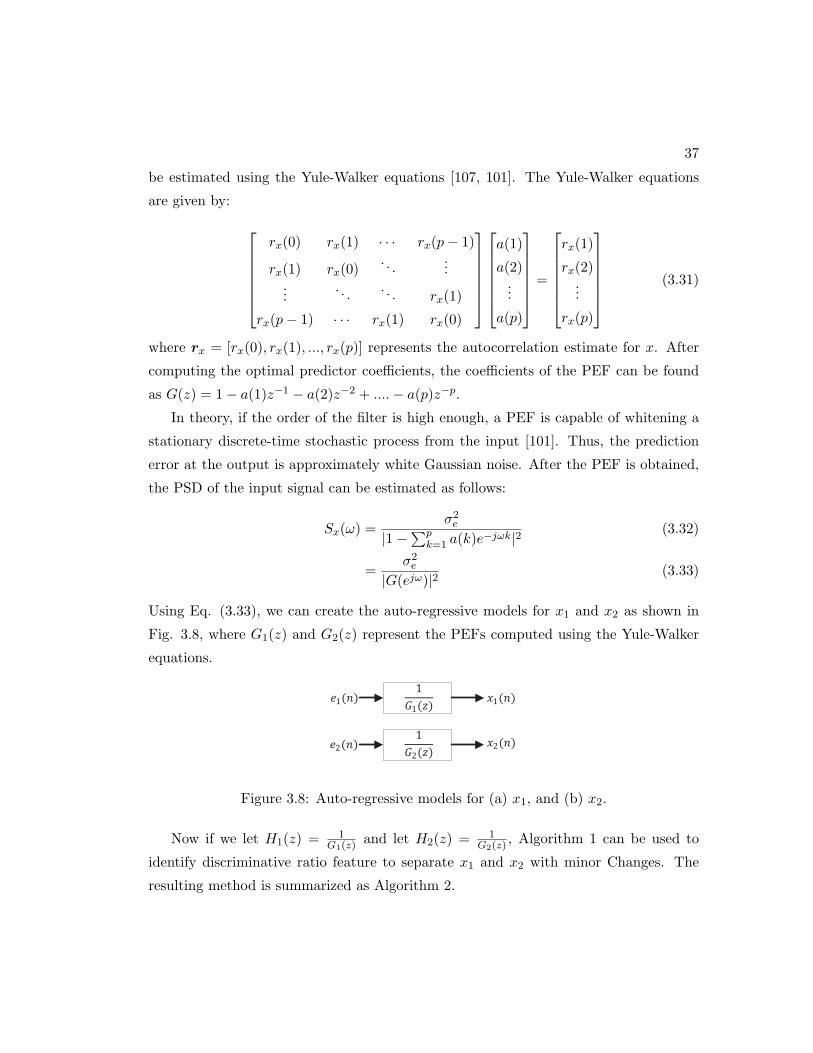
37
be estimated using the Yule-Walker equations [107, 101]. The Yule-Walker equations
are given by:
rx(0) rx(1) · · · rx(p− 1)
rx(1) rx(0). . .
......
. . .. . . rx(1)
rx(p− 1) · · · rx(1) rx(0)
a(1)
a(2)...
a(p)
=
rx(1)
rx(2)...
rx(p)
(3.31)
where rx = [rx(0), rx(1), ..., rx(p)] represents the autocorrelation estimate for x. After
computing the optimal predictor coefficients, the coefficients of the PEF can be found
as G(z) = 1− a(1)z−1 − a(2)z−2 + ....− a(p)z−p.
In theory, if the order of the filter is high enough, a PEF is capable of whitening a
stationary discrete-time stochastic process from the input [101]. Thus, the prediction
error at the output is approximately white Gaussian noise. After the PEF is obtained,
the PSD of the input signal can be estimated as follows:
Sx(ω) =σ2e
|1−∑p
k=1 a(k)e−jωk|2
(3.32)
=σ2e
|G(ejω)|2(3.33)
Using Eq. (3.33), we can create the auto-regressive models for x1 and x2 as shown in
Fig. 3.8, where G1(z) and G2(z) represent the PEFs computed using the Yule-Walker
equations.
1(!) "1(!) 1
#1($)
2(!) "2(!) 1
#2($)
Figure 3.8: Auto-regressive models for (a) x1, and (b) x2.
Now if we let H1(z) = 1G1(z)
and let H2(z) = 1G2(z)
, Algorithm 1 can be used to
identify discriminative ratio feature to separate x1 and x2 with minor Changes. The
resulting method is summarized as Algorithm 2.

38
Algorithm 2 Algorithm for identifying discriminative spectral power ratios using PEFs
(1) Compute the PEFs G1(z) and G2(z) for x1 and x2, respectively
(2) Plot the PEF ratio as RH(ejω) = |H2(ejω)||H1(ejω)| =
|G1(ejω)||G2(ejω)|
(3) Identify the frequency band 1 as B1 where RH(ejω) > 1(4) Identify the frequency band 2 as B2 where RH(ejω) < 1(5) Compute the band power in frequency band 1 as Px(B1)(6) Compute the band power in frequency band 2 as Px(B2)(7) Compute the spectral power ratio between the power in B1 and the power in B2
as Rx(B1, B2) = Px(B1)Px(B2)
for each state
3.3 Experimental Results
3.3.1 Synthesized Data
First, we synthesize a signal as the output of an autoregressive process of order 19
(AR(19)) driven by white Gaussian noise as shown in Fig. 3.1, where H1(z) = 1G1(z)
and H2(z) =1
G2(z). Thus, we can synthesize the signal data according to the following
euqations:
s1(n) = w(n)+
19∑i=1
a1(i)s1(n− i) (3.34)
x1(n) = s1(n) + v1(n) (3.35)
s2(n) = w(n)+
19∑i=1
a2(i)s2(n− i) (3.36)
x2(n) = s2(n) + v2(n) (3.37)
(3.38)
Let G1(z) = 1 − a1(1)z−1 − .... − a1(p)z
−p and G2(z) = 1 − a2(1)z−1 − .... − a2(p)z
−p
represent the PEFs for State 1 and State 2, respectively. Suppose that G1(z) and G2(z)
have frequency responses whose magnitudes are illustrated in Fig. 3.9.
Following the proposed method in Algorithm 2, we can compute and identify the
following variables:
(1) Compute the ratio PEF ratio as RH(ejω) = |H2(ejω)||H1(ejω)| =
|G1(ejω)||G2(ejω)| . Fig. 3.10 plots the
RH(ejω) versus frequency ω, where the blue horizontal line represents the value of 1.
(2) As shown in the figure, RH(ejω) > 1 when ω > 0.8π and RH(ejω) < 1 when
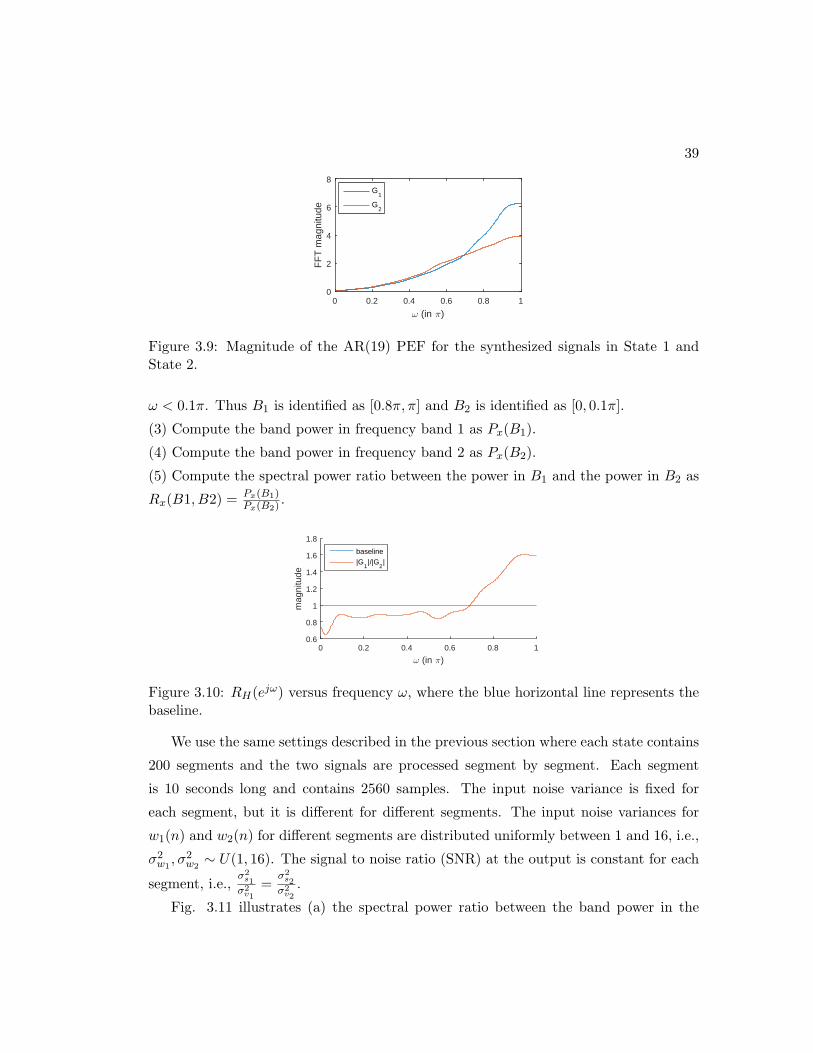
39
ω (in π)0 0.2 0.4 0.6 0.8 1
FF
T m
agni
tude
0
2
4
6
8G
1
G2
Figure 3.9: Magnitude of the AR(19) PEF for the synthesized signals in State 1 andState 2.
ω < 0.1π. Thus B1 is identified as [0.8π, π] and B2 is identified as [0, 0.1π].
(3) Compute the band power in frequency band 1 as Px(B1).
(4) Compute the band power in frequency band 2 as Px(B2).
(5) Compute the spectral power ratio between the power in B1 and the power in B2 as
Rx(B1, B2) = Px(B1)Px(B2)
.
ω (in π)0 0.2 0.4 0.6 0.8 1
mag
nitu
de
0.6
0.8
1
1.2
1.4
1.6
1.8
baseline|G
1|/|G
2|
Figure 3.10: RH(ejω) versus frequency ω, where the blue horizontal line represents thebaseline.
We use the same settings described in the previous section where each state contains
200 segments and the two signals are processed segment by segment. Each segment
is 10 seconds long and contains 2560 samples. The input noise variance is fixed for
each segment, but it is different for different segments. The input noise variances for
w1(n) and w2(n) for different segments are distributed uniformly between 1 and 16, i.e.,
σ2w1, σ2
w2∼ U(1, 16). The signal to noise ratio (SNR) at the output is constant for each
segment, i.e.,σ2s1
σ2v1
=σ2s2
σ2v2
.
Fig. 3.11 illustrates (a) the spectral power ratio between the band power in the
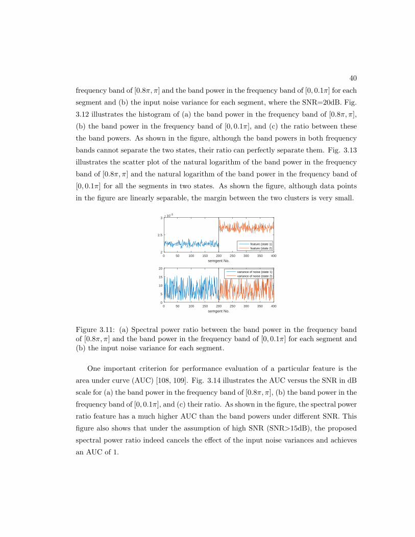
40
frequency band of [0.8π, π] and the band power in the frequency band of [0, 0.1π] for each
segment and (b) the input noise variance for each segment, where the SNR=20dB. Fig.
3.12 illustrates the histogram of (a) the band power in the frequency band of [0.8π, π],
(b) the band power in the frequency band of [0, 0.1π], and (c) the ratio between these
the band powers. As shown in the figure, although the band powers in both frequency
bands cannot separate the two states, their ratio can perfectly separate them. Fig. 3.13
illustrates the scatter plot of the natural logarithm of the band power in the frequency
band of [0.8π, π] and the natural logarithm of the band power in the frequency band of
[0, 0.1π] for all the segments in two states. As shown the figure, although data points
in the figure are linearly separable, the margin between the two clusters is very small.
semgent No.0 50 100 150 200 250 300 350 400
×10-3
2
2.5
3
feature (state 1)feature (state 2)
semgent No.0 50 100 150 200 250 300 350 400
0
5
10
15
20variance of noise (state 1)variance of noise (state 2)
Figure 3.11: (a) Spectral power ratio between the band power in the frequency bandof [0.8π, π] and the band power in the frequency band of [0, 0.1π] for each segment and(b) the input noise variance for each segment.
One important criterion for performance evaluation of a particular feature is the
area under curve (AUC) [108, 109]. Fig. 3.14 illustrates the AUC versus the SNR in dB
scale for (a) the band power in the frequency band of [0.8π, π], (b) the band power in the
frequency band of [0, 0.1π], and (c) their ratio. As shown in the figure, the spectral power
ratio feature has a much higher AUC than the band powers under different SNR. This
figure also shows that under the assumption of high SNR (SNR>15dB), the proposed
spectral power ratio indeed cancels the effect of the input noise variances and achieves
an AUC of 1.
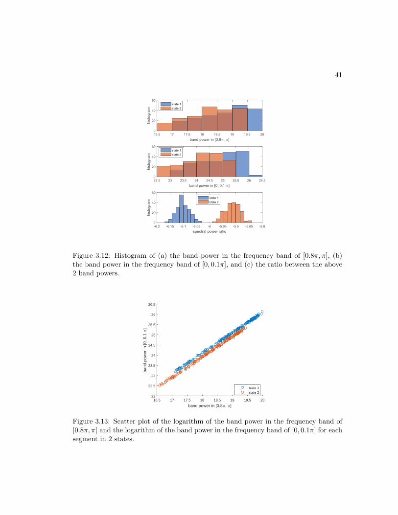
41
band power in [0.8 , ]
16.5 17 17.5 18 18.5 19 19.5 20
his
togra
m
0
20
40
60state 1
state 2
band power in [0, 0.1 ]
22.5 23 23.5 24 24.5 25 25.5 26 26.5
his
togra
m
0
20
40
60state 1
state 2
spectral power ratio
-6.2 -6.15 -6.1 -6.05 -6 -5.95 -5.9 -5.85 -5.8
his
togra
m
0
20
40
60
state 1
state 2
Figure 3.12: Histogram of (a) the band power in the frequency band of [0.8π, π], (b)the band power in the frequency band of [0, 0.1π], and (c) the ratio between the above2 band powers.
band power in [0.8π, π]16.5 17 17.5 18 18.5 19 19.5 20
band
pow
er in
[0, 0
.1 π
]
22
22.5
23
23.5
24
24.5
25
25.5
26
26.5
state 1state 2
Figure 3.13: Scatter plot of the logarithm of the band power in the frequency band of[0.8π, π] and the logarithm of the band power in the frequency band of [0, 0.1π] for eachsegment in 2 states.

42
SNR (in dB)0 5 10 15 20
AU
C
0
0.2
0.4
0.6
0.8
1
ratio fetureband power in [0, 0.2π]band power in [0.8π, π]
Figure 3.14: AUC versus the SNR in dB scale for the band power in the frequency bandof [0.8π, π], the band power in the frequency band of [0, 0.1π], and their ratio..
3.3.2 Improvement by Kalman Filter for Low SNR Environments
To further remove the fluctuations and noises of the spectral power ratios when SNR is
low, we propose to use a second-order Kalman filter to improve the results. The noise
of a process, which degrades the prediction capabilities, can be reduced by smoothing
its irregular effects. Kalman filter was shown in [22] to be very effective in smoothing
undesired fluctuations. The Kalman filter is a statistical method that can estimate
the state of a linear system by minimizing the variance of the estimation error, so the
estimates tend to be close to the true values of measurements. In order to apply the
Kalman filter to remove the noise from a signal, the process must be described as a linear
system. We propose to apply the same state-space model as the model described in [50]
and in supplementary document of [22] to the spectral power ratio features. Detailed
algorithm for a second-order Kalman filter is described in [101].
Fig. 3.15 illustrates the same spectral power ratio between the band power in the
frequency band of [0.8π, π] and the band power in the frequency band of [0, 0.1π] as
shown in Fig. 3.11 for State 1 and State 2, before and after post-processing in a low-
SNR case, where SNR=2dB. As shown in the figure, the ratio feature without Kalman
filter has many irregular fluctuations when SNR is low. However, Kalman fitler generates
a much smoother output feature and amplifies the differences between different states.
The AUC is improved from 0.7936 to 0.9980 after the Kalman filter is applied.
Fig. 3.16 illustrates the AUC versus the SNR in dB scale for the band power in the
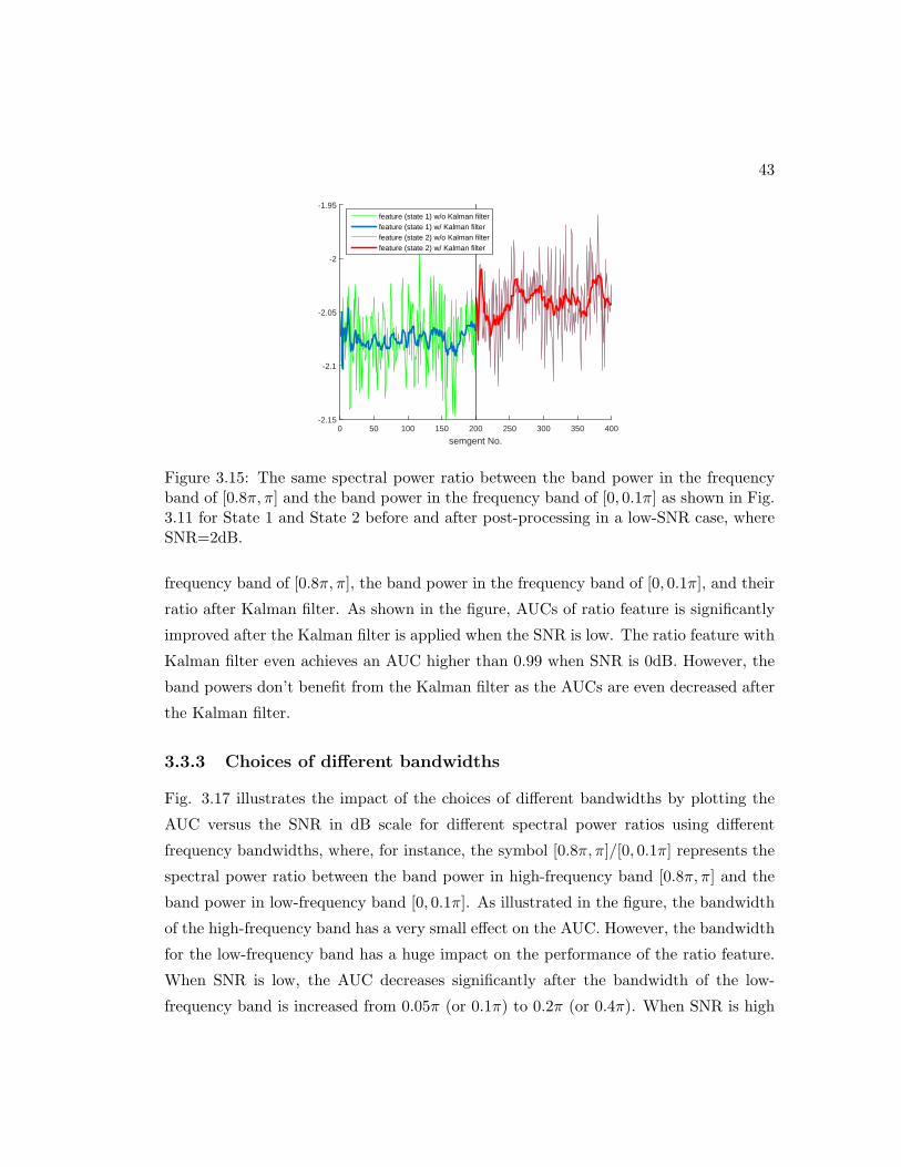
43
semgent No.0 50 100 150 200 250 300 350 400
-2.15
-2.1
-2.05
-2
-1.95feature (state 1) w/o Kalman filterfeature (state 1) w/ Kalman filterfeature (state 2) w/o Kalman filterfeature (state 2) w/ Kalman filter
Figure 3.15: The same spectral power ratio between the band power in the frequencyband of [0.8π, π] and the band power in the frequency band of [0, 0.1π] as shown in Fig.3.11 for State 1 and State 2 before and after post-processing in a low-SNR case, whereSNR=2dB.
frequency band of [0.8π, π], the band power in the frequency band of [0, 0.1π], and their
ratio after Kalman filter. As shown in the figure, AUCs of ratio feature is significantly
improved after the Kalman filter is applied when the SNR is low. The ratio feature with
Kalman filter even achieves an AUC higher than 0.99 when SNR is 0dB. However, the
band powers don’t benefit from the Kalman filter as the AUCs are even decreased after
the Kalman filter.
3.3.3 Choices of different bandwidths
Fig. 3.17 illustrates the impact of the choices of different bandwidths by plotting the
AUC versus the SNR in dB scale for different spectral power ratios using different
frequency bandwidths, where, for instance, the symbol [0.8π, π]/[0, 0.1π] represents the
spectral power ratio between the band power in high-frequency band [0.8π, π] and the
band power in low-frequency band [0, 0.1π]. As illustrated in the figure, the bandwidth
of the high-frequency band has a very small effect on the AUC. However, the bandwidth
for the low-frequency band has a huge impact on the performance of the ratio feature.
When SNR is low, the AUC decreases significantly after the bandwidth of the low-
frequency band is increased from 0.05π (or 0.1π) to 0.2π (or 0.4π). When SNR is high
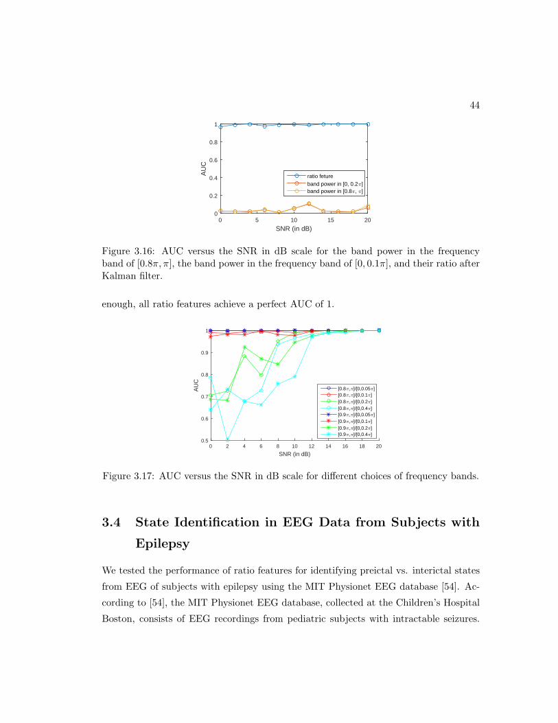
44
SNR (in dB)0 5 10 15 20
AU
C
0
0.2
0.4
0.6
0.8
1
ratio fetureband power in [0, 0.2π]band power in [0.8π, π]
Figure 3.16: AUC versus the SNR in dB scale for the band power in the frequencyband of [0.8π, π], the band power in the frequency band of [0, 0.1π], and their ratio afterKalman filter.
enough, all ratio features achieve a perfect AUC of 1.
SNR (in dB)0 2 4 6 8 10 12 14 16 18 20
AU
C
0.5
0.6
0.7
0.8
0.9
1
[0.8π,π]/[0,0.05π][0.8π,π]/[0,0.1π][0.8π,π]/[0,0.2π][0.8π,π]/[0,0.4π][0.9π,π]/[0,0.05π][0.9π,π]/[0,0.1π][0.9π,π]/[0,0.2π][0.9π,π]/[0,0.4π]
Figure 3.17: AUC versus the SNR in dB scale for different choices of frequency bands.
3.4 State Identification in EEG Data from Subjects with
Epilepsy
We tested the performance of ratio features for identifying preictal vs. interictal states
from EEG of subjects with epilepsy using the MIT Physionet EEG database [54]. Ac-
cording to [54], the MIT Physionet EEG database, collected at the Children’s Hospital
Boston, consists of EEG recordings from pediatric subjects with intractable seizures.
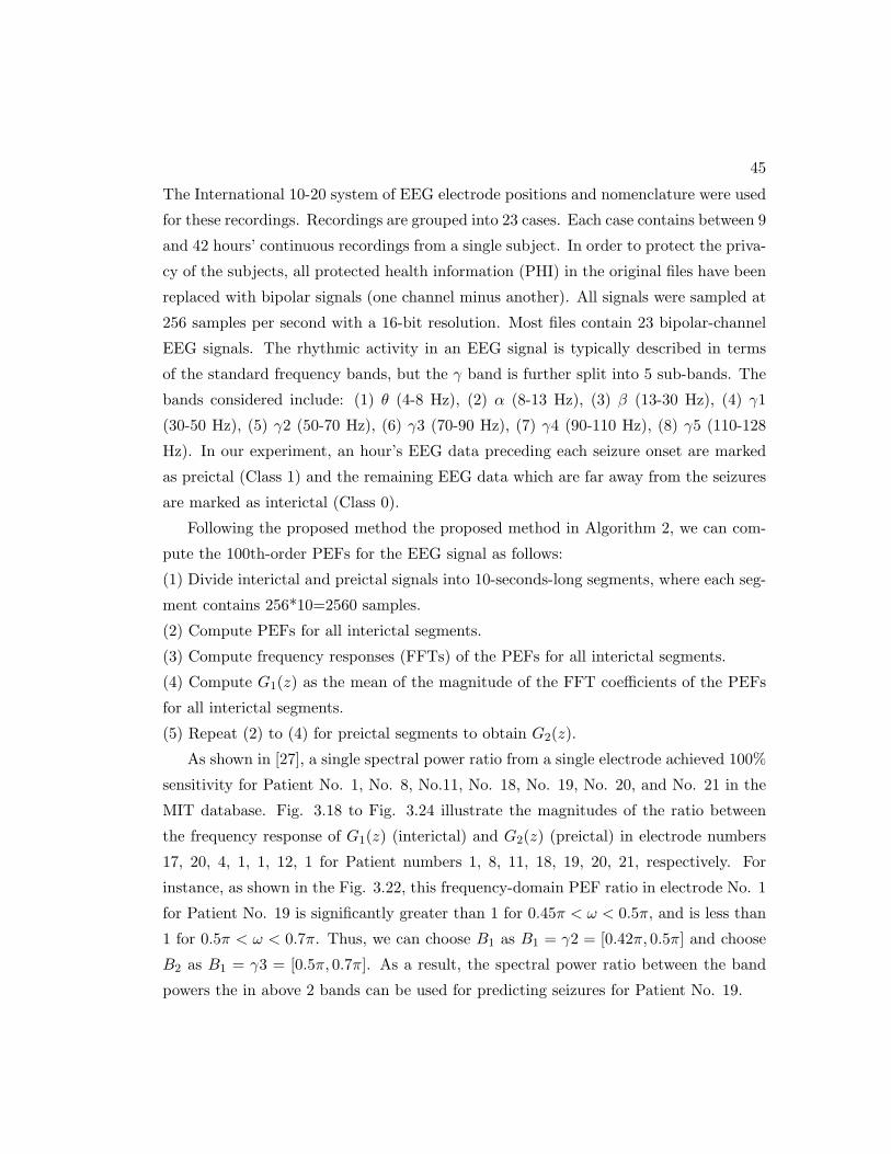
45
The International 10-20 system of EEG electrode positions and nomenclature were used
for these recordings. Recordings are grouped into 23 cases. Each case contains between 9
and 42 hours’ continuous recordings from a single subject. In order to protect the priva-
cy of the subjects, all protected health information (PHI) in the original files have been
replaced with bipolar signals (one channel minus another). All signals were sampled at
256 samples per second with a 16-bit resolution. Most files contain 23 bipolar-channel
EEG signals. The rhythmic activity in an EEG signal is typically described in terms
of the standard frequency bands, but the γ band is further split into 5 sub-bands. The
bands considered include: (1) θ (4-8 Hz), (2) α (8-13 Hz), (3) β (13-30 Hz), (4) γ1
(30-50 Hz), (5) γ2 (50-70 Hz), (6) γ3 (70-90 Hz), (7) γ4 (90-110 Hz), (8) γ5 (110-128
Hz). In our experiment, an hour’s EEG data preceding each seizure onset are marked
as preictal (Class 1) and the remaining EEG data which are far away from the seizures
are marked as interictal (Class 0).
Following the proposed method the proposed method in Algorithm 2, we can com-
pute the 100th-order PEFs for the EEG signal as follows:
(1) Divide interictal and preictal signals into 10-seconds-long segments, where each seg-
ment contains 256*10=2560 samples.
(2) Compute PEFs for all interictal segments.
(3) Compute frequency responses (FFTs) of the PEFs for all interictal segments.
(4) Compute G1(z) as the mean of the magnitude of the FFT coefficients of the PEFs
for all interictal segments.
(5) Repeat (2) to (4) for preictal segments to obtain G2(z).
As shown in [27], a single spectral power ratio from a single electrode achieved 100%
sensitivity for Patient No. 1, No. 8, No.11, No. 18, No. 19, No. 20, and No. 21 in the
MIT database. Fig. 3.18 to Fig. 3.24 illustrate the magnitudes of the ratio between
the frequency response of G1(z) (interictal) and G2(z) (preictal) in electrode numbers
17, 20, 4, 1, 1, 12, 1 for Patient numbers 1, 8, 11, 18, 19, 20, 21, respectively. For
instance, as shown in the Fig. 3.22, this frequency-domain PEF ratio in electrode No. 1
for Patient No. 19 is significantly greater than 1 for 0.45π < ω < 0.5π, and is less than
1 for 0.5π < ω < 0.7π. Thus, we can choose B1 as B1 = γ2 = [0.42π, 0.5π] and choose
B2 as B1 = γ3 = [0.5π, 0.7π]. As a result, the spectral power ratio between the band
powers the in above 2 bands can be used for predicting seizures for Patient No. 19.
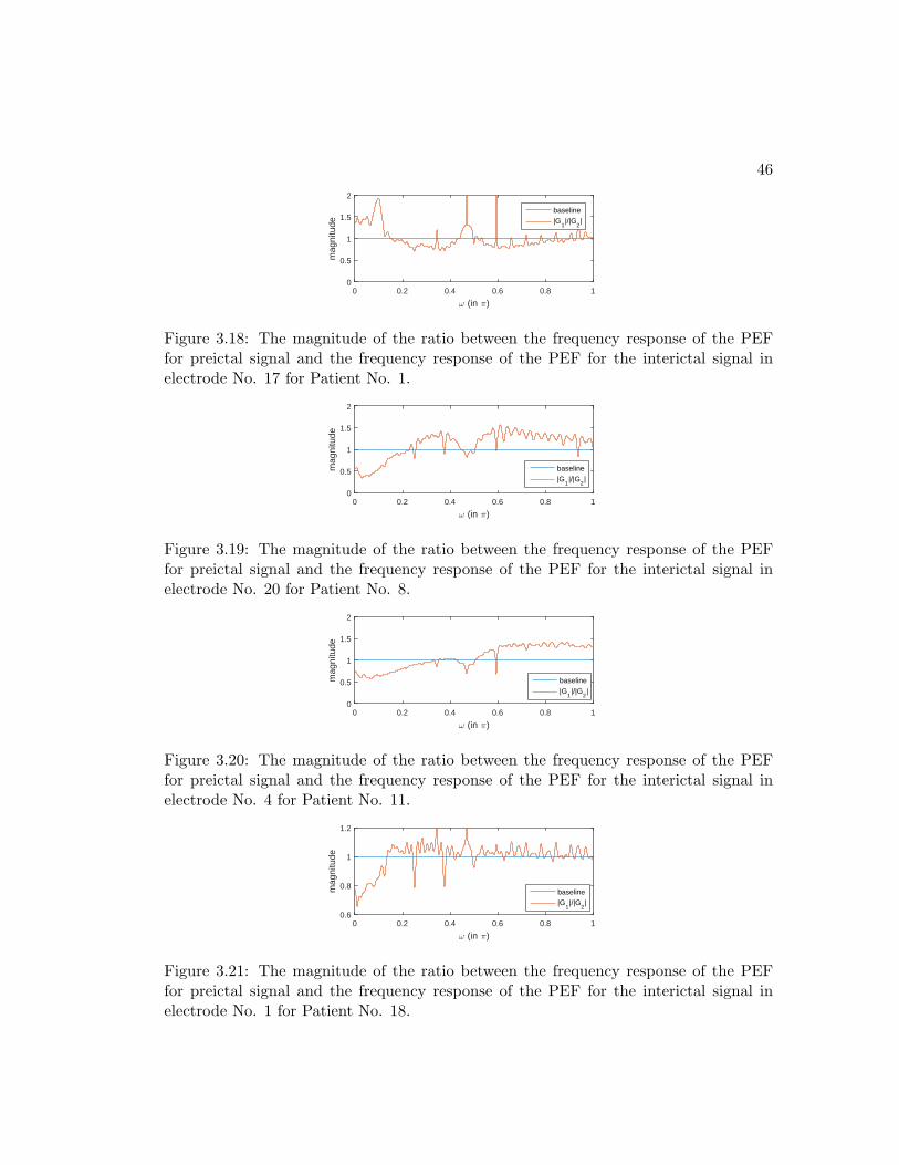
46
ω (in π)0 0.2 0.4 0.6 0.8 1
mag
nitu
de
0
0.5
1
1.5
2
baseline|G
1|/|G
2|
Figure 3.18: The magnitude of the ratio between the frequency response of the PEFfor preictal signal and the frequency response of the PEF for the interictal signal inelectrode No. 17 for Patient No. 1.
ω (in π)0 0.2 0.4 0.6 0.8 1
mag
nitu
de
0
0.5
1
1.5
2
baseline|G
1|/|G
2|
Figure 3.19: The magnitude of the ratio between the frequency response of the PEFfor preictal signal and the frequency response of the PEF for the interictal signal inelectrode No. 20 for Patient No. 8.
ω (in π)0 0.2 0.4 0.6 0.8 1
mag
nitu
de
0
0.5
1
1.5
2
baseline|G
1|/|G
2|
Figure 3.20: The magnitude of the ratio between the frequency response of the PEFfor preictal signal and the frequency response of the PEF for the interictal signal inelectrode No. 4 for Patient No. 11.
ω (in π)0 0.2 0.4 0.6 0.8 1
mag
nitu
de
0.6
0.8
1
1.2
baseline|G
1|/|G
2|
Figure 3.21: The magnitude of the ratio between the frequency response of the PEFfor preictal signal and the frequency response of the PEF for the interictal signal inelectrode No. 1 for Patient No. 18.
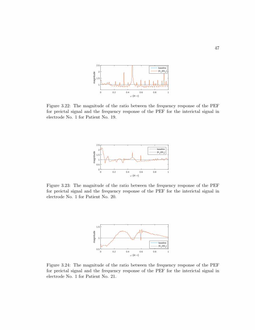
47
ω (in π)0 0.2 0.4 0.6 0.8 1
mag
nitu
de
1
1.5
2
2.5baseline|G
1|/|G
2|
Figure 3.22: The magnitude of the ratio between the frequency response of the PEFfor preictal signal and the frequency response of the PEF for the interictal signal inelectrode No. 1 for Patient No. 19.
ω (in π)0 0.2 0.4 0.6 0.8 1
mag
nitu
de
0
0.5
1
1.5
2
2.5
baseline|G
1|/|G
2|
Figure 3.23: The magnitude of the ratio between the frequency response of the PEFfor preictal signal and the frequency response of the PEF for the interictal signal inelectrode No. 1 for Patient No. 20.
ω (in π)0 0.2 0.4 0.6 0.8 1
mag
nitu
de
0.5
1
1.5
baseline|G
1|/|G
2|
Figure 3.24: The magnitude of the ratio between the frequency response of the PEFfor preictal signal and the frequency response of the PEF for the interictal signal inelectrode No. 1 for Patient No. 21.
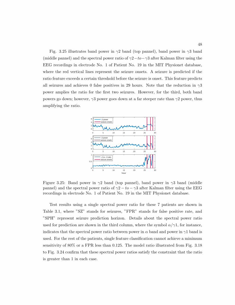
48
Fig. 3.25 illustrates band power in γ2 band (top pannel), band power in γ3 band
(middle pannel) and the spectral power ratio of γ2−to−γ3 after Kalman filter using the
EEG recordings in electrode No. 1 of Patient No. 19 in the MIT Physionet database,
where the red vertical lines represent the seizure onsets. A seizure is predicted if the
ratio feature exceeds a certain threshold before the seizure is onset. This feature predicts
all seizures and achieves 0 false positives in 29 hours. Note that the reduction in γ3
power amplies the ratio for the first two seizures. However, for the third, both band
powers go down; however, γ3 power goes down at a far steeper rate than γ2 power, thus
amplifying the ratio.
0 5 10 15 20 25 30
0
2
4
6γ2 powerseizure onsets
0 5 10 15 20 25 300
2
4
6 γ3 powerseizure onsets
hour0 5 10 15 20 25 30
0
0.5
1γ2-to-γ3 ratioseizure onsets
Figure 3.25: Band power in γ2 band (top pannel), band power in γ3 band (middlepannel) and the spectral power ratio of γ2− to− γ3 after Kalman filter using the EEGrecordings in electrode No. 1 of Patient No. 19 in the MIT Physionet database.
Test results using a single spectral power ratio for these 7 patients are shown in
Table 3.1, where ”SZ” stands for seizures, ”FPR” stands for false positive rate, and
”SPH” represent seizure prediction horizon. Details about the spectral power ratio
used for prediction are shown in the third column, where the symbol α/γ1, for instance,
indicates that the spectral power ratio between power in α band and power in γ1 band is
used. For the rest of the patients, single feature classification cannot achieve a minimum
sensitivity of 80% or a FPR less than 0.125. The model ratio illustrated from Fig. 3.18
to Fig. 3.24 confirm that these spectral power ratios satisfy the constraint that the ratio
is greater than 1 in each case.
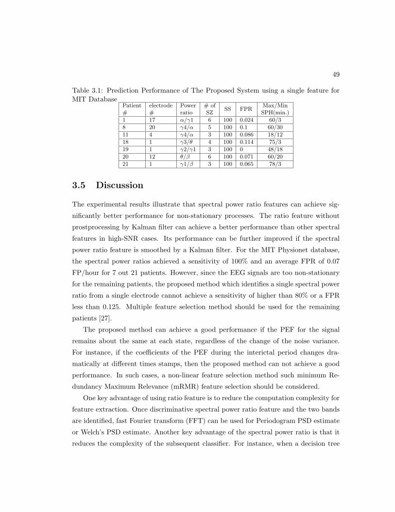
49
Table 3.1: Prediction Performance of The Proposed System using a single feature forMIT Database
Patient electrode Power # ofSS FPR
Max/Min# # ratio SZ SPH(min.)
1 17 α/γ1 6 100 0.024 60/3
8 20 γ4/α 5 100 0.1 60/30
11 4 γ4/α 3 100 0.086 18/12
18 1 γ3/θ 4 100 0.114 75/3
19 1 γ2/γ1 3 100 0 48/18
20 12 θ/β 6 100 0.071 60/20
21 1 γ1/β 3 100 0.065 78/3
3.5 Discussion
The experimental results illustrate that spectral power ratio features can achieve sig-
nificantly better performance for non-stationary processes. The ratio feature without
prostprocessing by Kalman filter can achieve a better performance than other spectral
features in high-SNR cases. Its performance can be further improved if the spectral
power ratio feature is smoothed by a Kalman filter. For the MIT Physionet database,
the spectral power ratios achieved a sensitivity of 100% and an average FPR of 0.07
FP/hour for 7 out 21 patients. However, since the EEG signals are too non-stationary
for the remaining patients, the proposed method which identifies a single spectral power
ratio from a single electrode cannot achieve a sensitivity of higher than 80% or a FPR
less than 0.125. Multiple feature selection method should be used for the remaining
patients [27].
The proposed method can achieve a good performance if the PEF for the signal
remains about the same at each state, regardless of the change of the noise variance.
For instance, if the coefficients of the PEF during the interictal period changes dra-
matically at different times stamps, then the proposed method can not achieve a good
performance. In such cases, a non-linear feature selection method such minimum Re-
dundancy Maximum Relevance (mRMR) feature selection should be considered.
One key advantage of using ratio feature is to reduce the computation complexity for
feature extraction. Once discriminative spectral power ratio feature and the two bands
are identified, fast Fourier transform (FFT) can be used for Periodogram PSD estimate
or Welch’s PSD estimate. Another key advantage of the spectral power ratio is that it
reduces the complexity of the subsequent classifier. For instance, when a decision tree

50
is used to separate the data points as shown in Fig. 3.13, large number of nodes are
needed as each node can only evaluate a single threshold. Using the ratio feature, a
single threshold is sufficient to separate the 2 classes.
3.6 Conclusion
In [36], several ratio features were identified to discriminate schizophrenia subjects from
healthy control from MEG. It can be verified that the selected bands indeed satisfy the
constraints of the frequency-domain model ratio. This paper proves the significance of
spectral power ratio between the band powers in two different frequency bands because
such a feature cancels the effect of the non-stationarity caused by the dramatic change
in the noise power when the signal-to-noise ratio (SNR) is high. When the SNR is
low, the performance of the spectral power ratios can be improved significantly if a
postprocessing step such as a second-order Kalman filter is applied. Experimental results
using synthesized data and the MIT Physionet database illustrate that the spectral
power ratios can achieve a much better performance than traditional spectral features.
This paper has derived a theory of the ratio of spectral power for a single time-series that
can span two states. However, in many applications, multiple time-series are available.
Future work will be directed towards deriving theory of ratio of spectral or cross-spectral
power for multi-channel applications.

Chapter 4
Seizure Detection from
Long-Term EEG Recordings
using Regression Tree Based
Feature Selection and Polynomial
SVM Classification
This chapter shows that combining the PSD features such as absolute spectral powers,
relative spectral powers and spectral power ratios as a feature set and then carefully
selecting a small number of these features from three or four electrodes can achieve a
better detection performance with low detection horizon. In the proposed approach [29],
we first compute the spectrogram of the input fragmented EEG signals from three or four
electrodes. Spectral powers and spectral ratios are extracted as features. The features
are then subjected to feature selection using classification and regression tree (CART).
The selected features are then subjected to a polynomial support vector machine (SVM)
classifier with degree of 2. Since all these features can be extracted by performing the
fast Fourier transform (FFT) on the signals and the classifier requires low hardware
complexity [97], the proposed algorithm can be implemented by the hardware with low
complexity and low power consumption.
51

52
4.1 Materials and Methods
4.1.1 Patients Database
The dataset for testing the proposed algorithm is from the UPenn and Mayo Clinic’s
Seizure Detection Challenge database [110]. The experimental procedures involving
human subjects were approved by the Institutional Review Board. The Institutions
Ethical Review Board approved all experimental procedures involving human subjects.
The experimental procedures involving animal models were approved by the Institu-
tional Animal Care and Ethics Committee.
According to [110], intracranial EEG was recorded from dogs with naturally oc-
curring epilepsy using an ambulatory monitoring system. EEG was sampled from 16
electrodes at 400 Hz, and recorded voltages were referenced to the group average. The
canine data are from an implanted device acquiring data from 16 subdural electrodes
[111]. Two 4-contact strips are implanted over each hemisphere in an antero-posterior
orientation. In addition, datasets from patients with epilepsy undergoing intracranial
EEG monitoring to identify a region of the brain that can be resected to prevent future
seizures are included [112]. These datasets have varying numbers of electrodes and are
sampled at 500 Hz or 5000 Hz, with recorded voltages referenced to an electrode out-
side the brain. The human data are from patients with temporal and extra-temporal
lobe epilepsy undergoing evaluation for epilepsy surgery. The iEEG recordings are from
depth electrodes implanted along anterior-posterior axis of hippocampus, and from sub-
dural electrode grids in various locations.
The training data is organized into 1-second EEG clips labeled ”Ictal” for seizure
data segments, or ”Interictal” for non-seizure data segments. Training data are arranged
sequentially while testing data are in random order. Ictal training and testing data
segments are provided covering the entire seizure, while interictal data segments are
provided covering approximately the mean seizure duration for each subject. Starting
points for the interictal data segments were chosen randomly from the full data record,
with the restriction that no interictal segment be less than one hour before or after a
seizure.
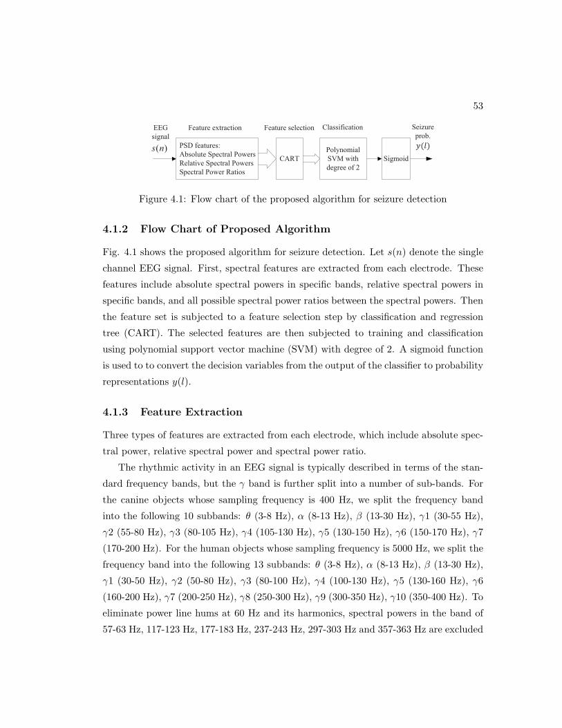
53
EEG
signal
Feature extraction
)(ns PSD features:
Absolute Spectral Powers
Relative Spectral Powers
Spectral Power Ratios
CART
Feature selection
Polynomial
SVM with
degree of 2
Classification
Sigmoid
Seizure
prob.
Figure 4.1: Flow chart of the proposed algorithm for seizure detection
4.1.2 Flow Chart of Proposed Algorithm
Fig. 4.1 shows the proposed algorithm for seizure detection. Let s(n) denote the single
channel EEG signal. First, spectral features are extracted from each electrode. These
features include absolute spectral powers in specific bands, relative spectral powers in
specific bands, and all possible spectral power ratios between the spectral powers. Then
the feature set is subjected to a feature selection step by classification and regression
tree (CART). The selected features are then subjected to training and classification
using polynomial support vector machine (SVM) with degree of 2. A sigmoid function
is used to to convert the decision variables from the output of the classifier to probability
representations y(l).
4.1.3 Feature Extraction
Three types of features are extracted from each electrode, which include absolute spec-
tral power, relative spectral power and spectral power ratio.
The rhythmic activity in an EEG signal is typically described in terms of the stan-
dard frequency bands, but the γ band is further split into a number of sub-bands. For
the canine objects whose sampling frequency is 400 Hz, we split the frequency band
into the following 10 subbands: θ (3-8 Hz), α (8-13 Hz), β (13-30 Hz), γ1 (30-55 Hz),
γ2 (55-80 Hz), γ3 (80-105 Hz), γ4 (105-130 Hz), γ5 (130-150 Hz), γ6 (150-170 Hz), γ7
(170-200 Hz). For the human objects whose sampling frequency is 5000 Hz, we split the
frequency band into the following 13 subbands: θ (3-8 Hz), α (8-13 Hz), β (13-30 Hz),
γ1 (30-50 Hz), γ2 (50-80 Hz), γ3 (80-100 Hz), γ4 (100-130 Hz), γ5 (130-160 Hz), γ6
(160-200 Hz), γ7 (200-250 Hz), γ8 (250-300 Hz), γ9 (300-350 Hz), γ10 (350-400 Hz). To
eliminate power line hums at 60 Hz and its harmonics, spectral powers in the band of
57-63 Hz, 117-123 Hz, 177-183 Hz, 237-243 Hz, 297-303 Hz and 357-363 Hz are excluded

54
in spectral power computation.
For canine objects, all possible combinations of ten spectral powers lead to a total
number of(102
)= 45 ratios from a single channel EEG signal. For human patients, that
number is increased to(132
)= 78.
Fig. 4.2 illustrates the normalized (between 0 and 1) absolute spectral power in band
[13, 30] Hz (top pannel), the spectral power in band [160, 200] Hz (middle pannel) and
the spectral power ratio of P8,13-to-P160,200 using the EEG recordings in electrode No.
10 of patient No. 8 from the Upenn and Mayo Clinic database, where the red vertical
lines represent the seizure onsets. While the spectral power features in both bands are
indiscriminate of the ictal and interictal periods, the ratio between them shows strong
detectability of the seizures as this ratio increases significantly after the seizure onsets.
0 200 400 600 800 1000 1200 1400 1600 1800 20000
0.5
1
second
e1
0,
P8,1
3/P
160,2
00
0 200 400 600 800 1000 1200 1400 1600 1800 20000
0.5
1
second
e1
0, P
8,1
3
0 200 400 600 800 1000 1200 1400 1600 1800 20000
0.5
1
second
e1
0,
P160,2
00
Figure 4.2: Spectral power in in band [13, 30] Hz (top pannel), spectral power in band[160, 200] Hz (middle pannel) and the spectral power ratio of P8,13-to-P160,200 using theEEG recordings in electrode No. 10 of patient No. 8 from the Upenn and Mayo Clinic’sdatabase.
4.1.4 Feature Selection by Regression Tree
A three-node regression tree is created using CART. Fig. 4.3 shows a regression tree
with 3 nodes for Patient No. 7 from the Upenn and Mayo Clinic’s database. This
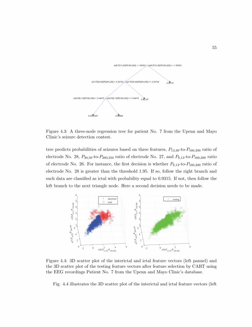
55
0.93151
0.92157
0.0046397 0.88889
e28,P[13,30]/P[160,200] < 1.95353
e27,P[30,50]/P[200,250] < 4.25702
e26,P[8,13]/P[160,200] < 3.44675
e28,P[13,30]/P[160,200] >= 1.95353
e27,P[30,50]/P[200,250] >= 4.25702
e26,P[8,13]/P[160,200] >= 3.44675
Figure 4.3: A three-node regression tree for patient No. 7 from the Upenn and MayoClinic’s seizure detection contest.
tree predicts probabilities of seizures based on three features, P13,30-to-P160,200 ratio of
electrode No. 28, P30,50-to-P200,250 ratio of electrode No. 27, and P8,13-to-P160,200 ratio
of electrode No. 26. For instance, the first decision is whether P8,13-to-P160,200 ratio of
electrode No. 28 is greater than the threshold 1.95. If so, follow the right branch and
such data are classified as ictal with probability equal to 0.9315. If not, then follow the
left branch to the next triangle node. Here a second decision needs to be made.
−2 0 2 4 60
2
4
6
1
2
3
4
5
6
e28,P13,30
/P160,200
e26,P8,13/P160,200
e27,P30,50/P200,250
interictal
ictal
−2 0 2 40
2
4
6
1
2
3
4
5
6
e28,P13,30
/P160,200
e26,P8,13/P160,200
e27,P30,50/P200,250
testing
Figure 4.4: 3D scatter plot of the interictal and ictal feature vectors (left pannel) andthe 3D scatter plot of the testing feature vectors after feature selection by CART usingthe EEG recordings Patient No. 7 from the Upenn and Mayo Clinic’s database.
Fig. 4.4 illustrates the 3D scatter plot of the interictal and ictal feature vectors (left

56
pannel) and the 3D scatter plot of the testing feature vectors after feature selection by
CART using the EEG recordings of Patient No. 7 from the Upenn and Mayo Clinic
database, where the blue cross dots represent the interictal feature vectros, the red
circled dots represent the ictal feature vectors, and the green circled dots represent the
testing feature vectors.
4.1.5 Seizure Detection Classification
As CART unveils nonlinear relationships, polynomial SVM with degree of 2 is used.
After computing the decision variable, a sigmoid function, S(p(t − c)), is used to
convert its values into probabilities, where c represents the center of the function and
p represents spread of the function, respectively. Fig. 4.5 illustrates the input decision
variable and output seizure probability of the sigmoid function.
0 200 400 600 800 1000 1200 1400 1600 1800 20000
0.5
1decision variable
seizue onsets
0 200 400 600 800 1000 1200 1400 1600 1800 20000
0.5
1
second
seizure probability
seizue onsets
Figure 4.5: Conversion form decision variable to seizure probability for Pat. No. 8.
4.2 Experimental Results
Half of the training data are selected randomly for feature selection and training the
classifier. Parameters such as αi, b, p, and c are selected such that the probabilities of
the testing data achieve the maximum area under curve (AUC).
Test Results of the proposed algorithm are shown in Table 4.1, where ”SS” stands
for sensitivity and ’SZ’ stands for seizures. Details of the features used to detect seizures
are shown in the second column. For instance, three features are used for Patient No.

57
Table 4.1: Detection Performance of The Proposed SystemObject
Feature Details# of
SS AUCName SZ
Dog 1Electrode 3 8 16
5 100 0.9773Feature P80,105 P105,130
P80,105
P170,200
Dog 2Electrode 8 7 16
3 100 0.9975Feature
P3,8
P150,170
P3,8
P170,200
P3,8
P150,170
Dog 3Electrode 14 7 8
12 100 0.9876Feature P3,8 P13,30 P150,170
Dog 4Electrode 7 8 10 15
2 100 0.9549Feature P30,55 P55,80 Q150,170 P3,8
Pat. 1Electrode 19 19 6
2 100 0.9878Feature P105,130
P55,80
P170,200Q105,130
Pat. 2Electrode 1 4 4
3 100 0.9852Feature
P8,13
P350,400
P80,100
P160,200Q30,55
Pat. 3Electrode 5 13 35 9
7 100 0.9506Feature P3,8 P160,200 Q50,80
P50,80
P350,400
Pat. 4Electrode 36 36 36
2 100 1.0000Feature
P30,50
P80,100
P30,50
P100,130
P30,50
P130,160
Pat. 5Electrode 25 13 35 2
3 100 0.9723Feature P13,30 P50,80
P130,160
P350,400
P160,200
P350,400
Pat. 6Electrode 15 24 16
4 100 0.9973Feature
P3,8
P80,100
P8,13
P80,100
P8,13
P30,50
Pat. 7Electrode 28 27 26
3 100 0.9897Feature
P13,30
P160,200
P30,50
P200,250
P8,13
P200,250
Pat. 8Electrode 2 10 7
2 100 0.9818Feature P300,350
P8,13
P160,200
P8,13
P130,160
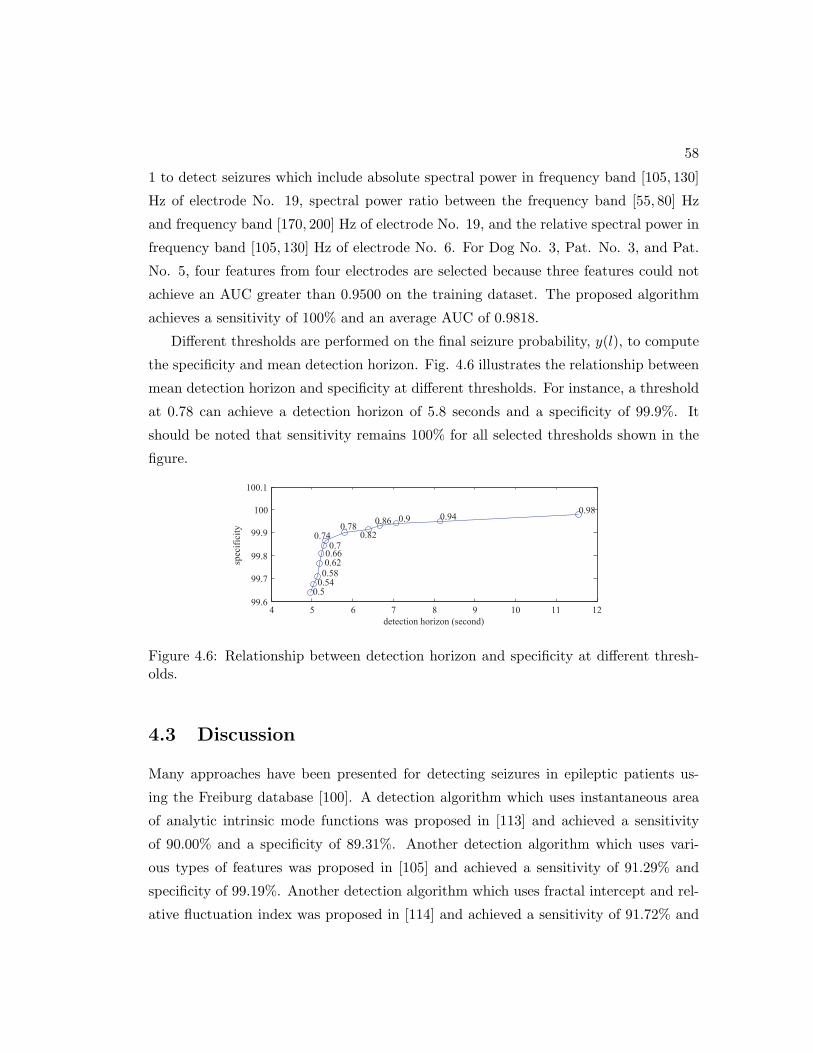
58
1 to detect seizures which include absolute spectral power in frequency band [105, 130]
Hz of electrode No. 19, spectral power ratio between the frequency band [55, 80] Hz
and frequency band [170, 200] Hz of electrode No. 19, and the relative spectral power in
frequency band [105, 130] Hz of electrode No. 6. For Dog No. 3, Pat. No. 3, and Pat.
No. 5, four features from four electrodes are selected because three features could not
achieve an AUC greater than 0.9500 on the training dataset. The proposed algorithm
achieves a sensitivity of 100% and an average AUC of 0.9818.
Different thresholds are performed on the final seizure probability, y(l), to compute
the specificity and mean detection horizon. Fig. 4.6 illustrates the relationship between
mean detection horizon and specificity at different thresholds. For instance, a threshold
at 0.78 can achieve a detection horizon of 5.8 seconds and a specificity of 99.9%. It
should be noted that sensitivity remains 100% for all selected thresholds shown in the
figure.
4 5 6 7 8 9 10 11 1299.6
99.7
99.8
99.9
100
100.1
0.50.540.580.620.66 0.7
0.740.78
0.82
0.86 0.9 0.940.98
detection horizon (second)
spec
ific
ity
Figure 4.6: Relationship between detection horizon and specificity at different thresh-olds.
4.3 Discussion
Many approaches have been presented for detecting seizures in epileptic patients us-
ing the Freiburg database [100]. A detection algorithm which uses instantaneous area
of analytic intrinsic mode functions was proposed in [113] and achieved a sensitivity
of 90.00% and a specificity of 89.31%. Another detection algorithm which uses vari-
ous types of features was proposed in [105] and achieved a sensitivity of 91.29% and
specificity of 99.19%. Another detection algorithm which uses fractal intercept and rel-
ative fluctuation index was proposed in [114] and achieved a sensitivity of 91.72% and
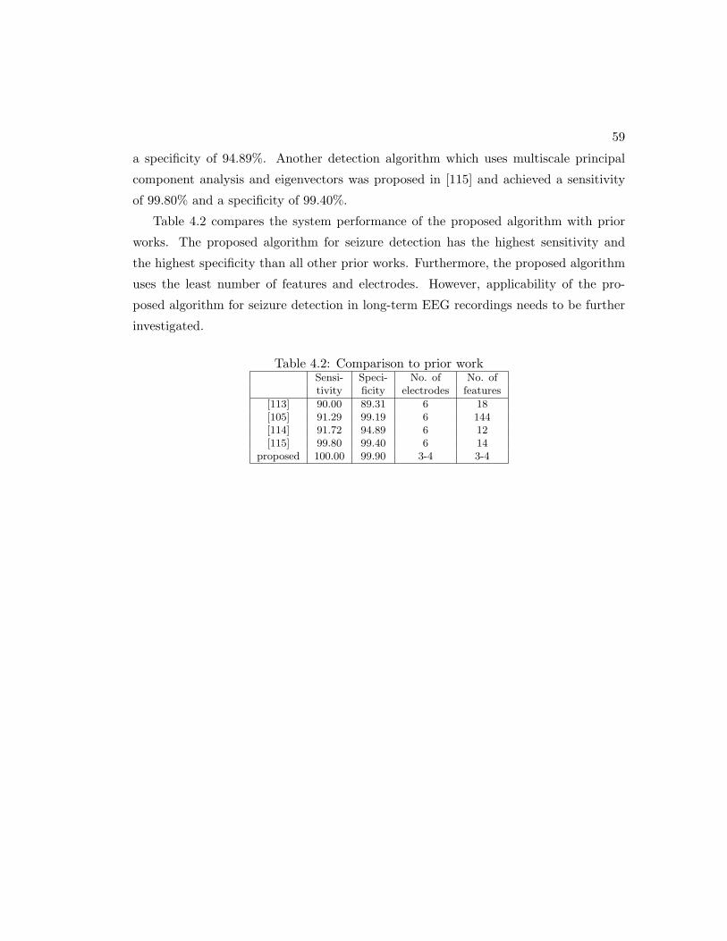
59
a specificity of 94.89%. Another detection algorithm which uses multiscale principal
component analysis and eigenvectors was proposed in [115] and achieved a sensitivity
of 99.80% and a specificity of 99.40%.
Table 4.2 compares the system performance of the proposed algorithm with prior
works. The proposed algorithm for seizure detection has the highest sensitivity and
the highest specificity than all other prior works. Furthermore, the proposed algorithm
uses the least number of features and electrodes. However, applicability of the pro-
posed algorithm for seizure detection in long-term EEG recordings needs to be further
investigated.
Table 4.2: Comparison to prior workSensi- Speci- No. of No. oftivity ficity electrodes features
[113] 90.00 89.31 6 18[105] 91.29 99.19 6 144[114] 91.72 94.89 6 12[115] 99.80 99.40 6 14
proposed 100.00 99.90 3-4 3-4
Chapter 5
Seizure Prediction from
Short-Term EEG Recordings
using Sparse Features
In low-power and low-complexity hardware design, the first key consideration is the
number of sensors used to collect EEG signals. Electrode selection is an essential step
before feature selection as sensors and analog-to-digital converters (A/D) can be highly
power consuming for an implantable or wearable biomedical device. The second key con-
sideration is selecting useful features that are computationally simple and are indicative
of upcoming seizure activities. The third key consideration is the choice of classifier.
Based on the selection of the classifier, a criteria for electrode and feature selection
should be chosen accordingly in order to achieve the best classification performance. It
is shown in [97] that linear classifiers have significantly lower power consumptions than
the nonlinear ones and are dependent on the feature dimensions only. Therefore, only
linear classifiers are considered. Thus, instead of selecting electrodes by their locations,
which has been used in other studies, we select electrodes and features in a way such that
the preictal features are as linearly separable from the interictal features as possible.
In the proposed approach [27], we first compute the spectrogram of the input EEG
signals from one or two electrodes. A window based PSD computation is used with
a 4-second sliding window with half overlap. Thus, the effective window period is 2
60

61
second. Spectral powers and spectral ratios are extracted as features and are input to a
classifier. A postprocessing step is used to remove undesired fluctuations of the decision
output of the classifier. The feature signals are then subjected to feature selection and
classification where two strategies are used. One is the single feature selection and the
other is the multi-dimensional feature selection. While a seizure prediction system using
a single feature requires low hardware complexity and power consumption, systems using
multi-dimensional features achieve a higher prediction reliability. Multi-dimensional
features are selected for patients where systems using a single feature can not achieve a
predetermined requirement.
5.1 Materials and Methods
5.1.1 EEG Databases
We have trained and tested our algorithm on the two databases: Freiburg intracranial
EEG (iEEG) database [100] and MIT Physionet scalp EEG (sEEG) database [54].
Details about the Freiburg intracranial EEG (iEEG) database are described in 2.1.1.
Details of the MIT Physionet scalp EEG (sEEG) database are described in 3.4.
For both databases, patients who have less than three seizures are not analyzed. The
reason for not including these patients is that training using preictal data from only one
seizure is likely to lead to a model overfitting to that particular seizure and may not be
able to predict the other ones. Therefore, at least two seizures must be selected in the
training set and another seizure is used for testing.
For both databases, we use the following categorization: 60 minutes’ recordings
preceding seizure onsets are categorized as preictal (C1); 3 minute’s and 30 minutes’
recordings postceding seizure onsets are categorized as ictal (C2) and post-ictal (C3),
respectively; the rest of the recordings are categorized as interictal (C0). The goal of
seizure prediction is to separate C1 from C0, regardless of C2 and C3.
5.1.2 Feature Extraction
This section describes the method for feature extraction, feature selection and postpro-
cessing, which include spectral power computation, spectral power ratio computation

62
and Kalman filter.
Window-based Signal Processing
The window size is chosen as four seconds (M = 4 ∗ fs) and each segment is categorized
as interictal (C0), preictal (C1), ictal (C2), or post-ictal (C3).
Spectral Power and Spectral Power Ratios
Three types of features are extracted from the windowed signal. These include absolute
spectral power, relative spectral power and spectral power ratio. The rhythmic activity
in an EEG signal is typically described in terms of the standard frequency bands, but
the γ band is further split into 5 sub-bands. The bands considered include: (1) θ (4-8
Hz), (2) α (8-13 Hz), (3) β (13-30 Hz), (4) γ1 (30-50 Hz), (5) γ2 (50-70 Hz), (6) γ3
(70-90 Hz), (7) γ4 (90-110 Hz), (8) γ5 (110-128 Hz). For Freiburg database, to eliminate
power line hums at 50 Hz and its harmonics, spectral powers in the band of 47-53 Hz
and 97-103 Hz are excluded in spectral power computation. For MIT database, spectral
powers in the band of 57-63 Hz and 117-123 Hz are excluded. For a single channel
EEG signal, all possible combinations of eight spectral powers lead to a total number
of(82
)= 28 possible ratios.
In summary, for each electrode, 44 features which include 8 absolute spectral power,
8 relative spectral powers and 28 spectral power ratios are extracted every 2 seconds.
The key advantage of spectral power ratio features over the spectral power features
is that certain ratio features are strong indicators of an upcoming seizure activity while
the latter are not indicative of such activity at all as the spectral power usually fluctu-
ates a lot during both interictal and preictal periods. The ratio feature amplifies the
simultaneous increase in the spectral power of one band and decrease in that of another
band. For instance, Fig. 5.1 illustrates the spectral power in γ2 band (top pannel),
the spectral power in γ1 band (middle pannel) and the spectral power ratio of γ2-to-γ1
after postprcossing using the EEG recordings in electrode No. 1 of Patient No. 19 in
the MIT Physionet database, where the red vertical lines represent the seizure onsets.
While the spectral power features in both bands are indiscriminate of the preictal and
interictal periods, the ratio between them shows strong predictability of the upcoming
seizure activities as this ratio always increases significantly prior to the seizure onsets.

63
0 5 10 15 20 25 300
2
4
6
8
γ1 power
seizure onsets
0 5 10 15 20 25 30
0
2
4
6γ2 power
seizure onsets
0 5 10 15 20 25 300
0.5
1
hour
γ2−to−γ1 ratio
seizure onsets
Figure 5.1: Spectral power in γ2 band (top pannel), spectral power in γ1 band (middlepannel) and the spectral power ratio of γ2-to-γ1 after postprcossing using the EEGrecordings in electrode No. 1 of Patient No. 19 in the MIT Physionet database.
Postprocessing
The noise of a process, which degrades the prediction capabilities, can be reduced by
smoothing its irregular effects. Kalman filter was shown in [22] to be very effective
in smoothing undesired fluctuations. The Kalman filter is a statistical method that
can estimate the state of a linear system by means of minimizing the variance of the
estimation error, so the estimates tend to be close to the true values of measurements.
In order to apply the Kalman filter to remove the noise from a signal, the process
must be described as a linear system. We use the same state-space model as the model
described in [50] and in supplementary document of [22]. Detailed algorithm for a
second-order Kalman filter is described in [101]. As a result, Kalman fitler generates a
much smoother output feature.
5.1.3 Single Feature Selection and Classification
Flow chart of a single feature selection is shown is Fig. 5.2, where f(l) represents the
l-th feature sample. The feature basis selection step is followed by electrode selection.
The best electrode is selected using scatter matrix method. A second round of feature
selection is performed to further reduce the number of features. The linear separability
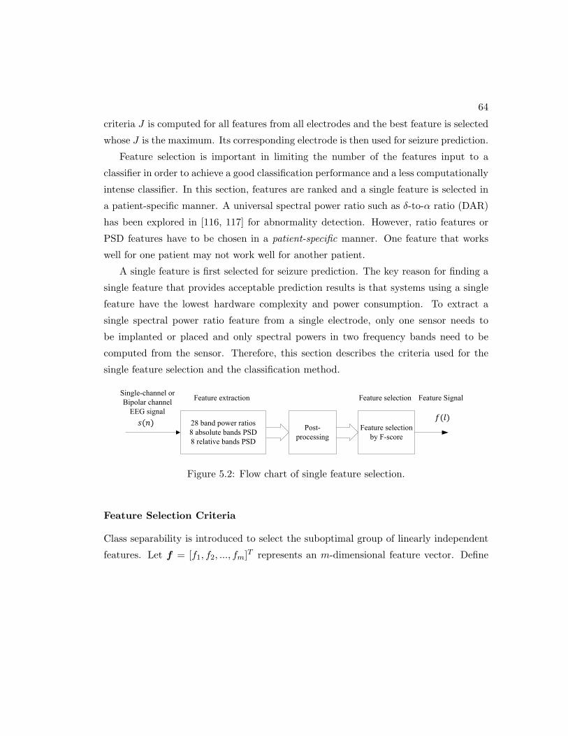
64
criteria J is computed for all features from all electrodes and the best feature is selected
whose J is the maximum. Its corresponding electrode is then used for seizure prediction.
Feature selection is important in limiting the number of the features input to a
classifier in order to achieve a good classification performance and a less computationally
intense classifier. In this section, features are ranked and a single feature is selected in
a patient-specific manner. A universal spectral power ratio such as δ-to-α ratio (DAR)
has been explored in [116, 117] for abnormality detection. However, ratio features or
PSD features have to be chosen in a patient-specific manner. One feature that works
well for one patient may not work well for another patient.
A single feature is first selected for seizure prediction. The key reason for finding a
single feature that provides acceptable prediction results is that systems using a single
feature have the lowest hardware complexity and power consumption. To extract a
single spectral power ratio feature from a single electrode, only one sensor needs to
be implanted or placed and only spectral powers in two frequency bands need to be
computed from the sensor. Therefore, this section describes the criteria used for the
single feature selection and the classification method.
Single-channel or
Bipolar channel
EEG signal
Feature selection
by F-score
Feature selection
Post-
processing
Feature Signal
28 band power ratios
8 absolute bands PSD
8 relative bands PSD
Feature extraction
Figure 5.2: Flow chart of single feature selection.
Feature Selection Criteria
Class separability is introduced to select the suboptimal group of linearly independent
features. Let f = [f1, f2, ..., fm]T represents an m-dimensional feature vector. Define

65
within-class scatter matrix (Sw) and between-class scatter matrix (Sb) as follows
Sw =
i=c∑i=1
piΣi (5.1)
Sb =
i=c∑i=1
pi(µi − µ0)(µi − µ0)T (5.2)
where c represents the number of classes, Σi = E[(f − µi)(f − µi)T ] represents the
covariance matrix for class i, pi represents the probability of class i, µ0 represents the
global mean vector, and µi represents the mean vector for class i, respectively. The
criterion
J =|Sw + Sb|
|Sw|(5.3)
takes a large positive value when samples in the m-dimensional space are well clustered
within each class, and the clusters of the different classes are well separated [5]. The
notation |A| represents the determinant of the matrix A. To select a single feature, J is
computed for all features from all electrodes and the feature that achieves the maximum
J is selected.
The application of the class separability criteria is illustrated for Patient No. 1 from
Freiburg database. For this patient, γ5-to-γ4 ratio of electrode No. 1 was selected as
the best feature. Fig. 5.3 illustrates the γ5-to-γ4 ratio of electrode No. 1 before and
after postprocessing using the (a) ictal and (b) interictal recordings of Patient No. 1 in
the Freiburg EEG database, where the blue curves represent the feature signals before
Kalman filter, the orange curves represent the outputs of the Kalman filter, and the
red lines represent the thresholds and the black dashed lines represent seizure onsets,
respectively. The feature in Fig. 3.15(a) corresponds to four different seizures where
each seizure onset occurs at exactly 3000 second time stamp. The feature in Fig. 3.15(b)
corresponds to interictal period of about 1 day duration. This particular ratio feature
is shown to be a good seizure predictor for this patient as the feature always exceeds
the threshold before seizure onset and is always below the threshold during interictal
period.
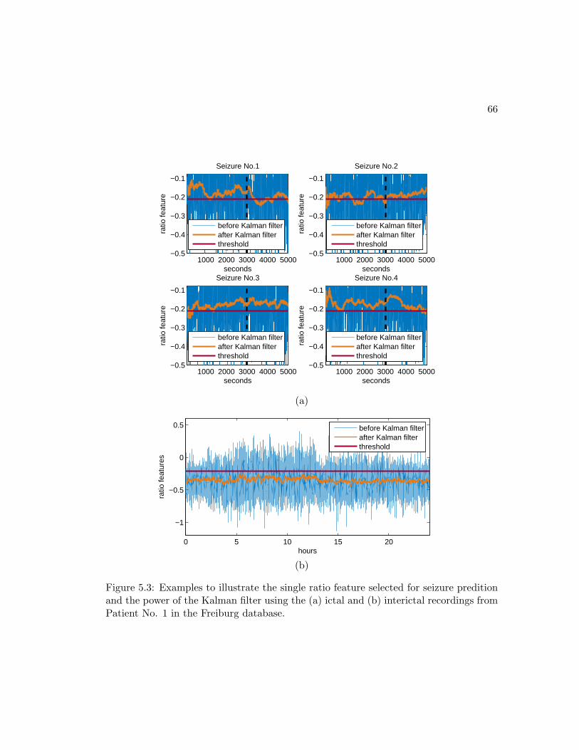
66
1000 2000 3000 4000 5000−0.5
−0.4
−0.3
−0.2
−0.1
seconds
ratio
feat
ure
Seizure No.1
1000 2000 3000 4000 5000−0.5
−0.4
−0.3
−0.2
−0.1
seconds
ratio
feat
ure
Seizure No.2
1000 2000 3000 4000 5000−0.5
−0.4
−0.3
−0.2
−0.1
seconds
ratio
feat
ure
Seizure No.3
1000 2000 3000 4000 5000−0.5
−0.4
−0.3
−0.2
−0.1
seconds
ratio
feat
ure
Seizure No.4
before Kalman filterafter Kalman filterthreshold
before Kalman filterafter Kalman filterthreshold
before Kalman filterafter Kalman filterthreshold
before Kalman filterafter Kalman filterthreshold
(a)
0 5 10 15 20
−1
−0.5
0
0.5
hours
ratio
feat
ures
before Kalman filterafter Kalman filterthreshold
(b)
Figure 5.3: Examples to illustrate the single ratio feature selected for seizure preditionand the power of the Kalman filter using the (a) ictal and (b) interictal recordings fromPatient No. 1 in the Freiburg database.
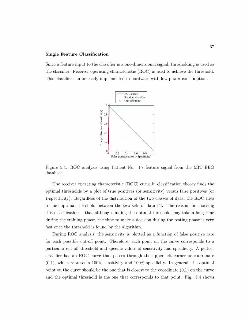
67
Single Feature Classification
Since a feature input to the classifier is a one-dimensional signal, thresholding is used as
the classifier. Receiver operating characteristic (ROC) is used to achieve the threshold.
This classifier can be easily implemented in hardware with low power consumption.
0 0.2 0.4 0.6 0.8 10
0.2
0.4
0.6
0.8
1
False positive rate (1−Specificity)
Tru
e po
sitiv
e ra
te (
Sen
sitiv
ity)
ROC curveRandom classifierCut−off point
Figure 5.4: ROC analysis using Patient No. 1’s feature signal from the MIT EEGdatabase.
The receiver operating characteristic (ROC) curve in classification theory finds the
optimal thresholds by a plot of true positives (or sensitivity) versus false positives (or
1-speciticity). Regardless of the distribution of the two classes of data, the ROC tries
to find optimal threshold between the two sets of data [5]. The reason for choosing
this classification is that although finding the optimal threshold may take a long time
during the training phase, the time to make a decision during the testing phase is very
fast once the threshold is found by the algorithm.
During ROC analysis, the sensitivity is plotted as a function of false positive rate
for each possible cut-off point. Therefore, each point on the curve corresponds to a
particular cut-off threshold and specific values of sensitivity and specificity. A perfect
classifier has an ROC curve that passes through the upper left corner or coordinate
(0,1), which represents 100% sensitivity and 100% specificity. In general, the optimal
point on the curve should be the one that is closest to the coordinate (0,1) on the curve
and the optimal threshold is the one that corresponds to that point. Fig. 5.4 shows
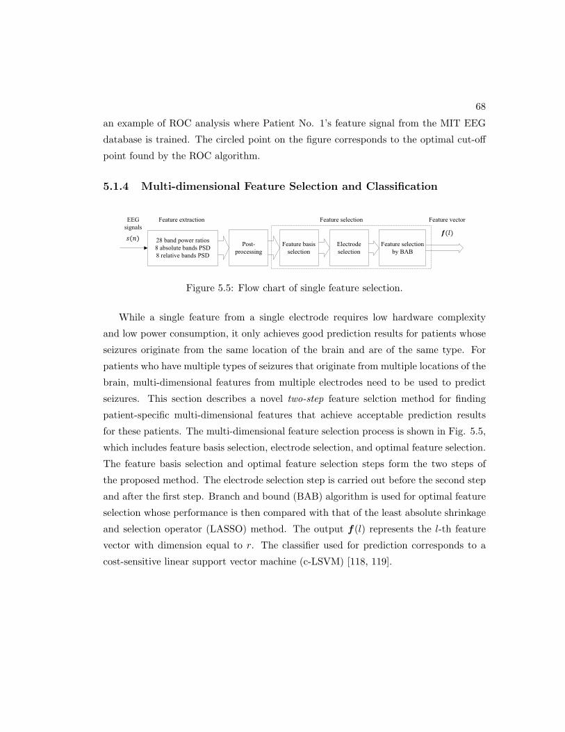
68
an example of ROC analysis where Patient No. 1’s feature signal from the MIT EEG
database is trained. The circled point on the figure corresponds to the optimal cut-off
point found by the ROC algorithm.
5.1.4 Multi-dimensional Feature Selection and Classification
EEG
signals
Feature selection
by BAB
Feature selection
Post-
processing
Feature vector
28 band power ratios
8 absolute bands PSD
8 relative bands PSD
Feature extraction
Feature basis
selection
Electrode
selection
Figure 5.5: Flow chart of single feature selection.
While a single feature from a single electrode requires low hardware complexity
and low power consumption, it only achieves good prediction results for patients whose
seizures originate from the same location of the brain and are of the same type. For
patients who have multiple types of seizures that originate from multiple locations of the
brain, multi-dimensional features from multiple electrodes need to be used to predict
seizures. This section describes a novel two-step feature selction method for finding
patient-specific multi-dimensional features that achieve acceptable prediction results
for these patients. The multi-dimensional feature selection process is shown in Fig. 5.5,
which includes feature basis selection, electrode selection, and optimal feature selection.
The feature basis selection and optimal feature selection steps form the two steps of
the proposed method. The electrode selection step is carried out before the second step
and after the first step. Branch and bound (BAB) algorithm is used for optimal feature
selection whose performance is then compared with that of the least absolute shrinkage
and selection operator (LASSO) method. The output f(l) represents the l-th feature
vector with dimension equal to r. The classifier used for prediction corresponds to a
cost-sensitive linear support vector machine (c-LSVM) [118, 119].
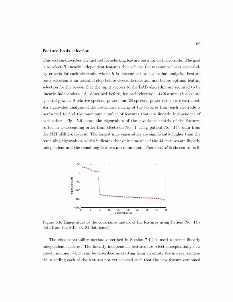
69
Feature basis selection
This section describes the method for selecting feature basis for each electrode. The goal
is to select R linearly independent features that achieve the maximum linear separabil-
ity criteria for each electrode, where R is determined by eigenvalue analysis. Feature
basis selection is an essential step before electrode selection and before optimal feature
selection for the reason that the input vectors to the BAB algorithm are required to be
linearly independent. As described before, for each electrode, 44 features (8 absolute
spectral powers, 8 relative spectral powers and 28 spectral power ratios) are extracted.
An eigenvalue analysis of the covariance matrix of the features from each electrode is
performed to find the maximum number of features that are linearly independent of
each other. Fig. 5.6 shows the eigenvalues of the covariance matrix of the features
sorted in a descending order from electrode No. 1 using patient No. 14’s data from
the MIT sEEG database. The largest nine eigenvalues are significantly higher than the
remaining eigenvalues, which indicates that only nine out of the 44 features are linearly
independent and the remaining features are redundant. Therefore, R is chosen to be 9.
0 5 10 15 20 25 30 35 40 45−200
−150
−100
−50
0
50
eigenvalue No
eige
nval
ue(d
B)
Figure 5.6: Eigenvalues of the covariance matrix of the features using Patient No. 14’sdata from the MIT sEEG database.)
The class separability method described in Section 7.1.2 is used to select linearly
independent features. The linearly independent features are selected sequentially in a
greedy manner, which can be described as starting from an empty feature set, sequen-
tially adding each of the features not yet selected such that the new feature combined

70
with the selected features maximizes the objective function J until R features are se-
lected. This process is repeated for each electrode. Such sequential selection scheme
will produce a suboptimal group of features that are linearly independent. Detailed
feature reduction scheme is described in Algorithm 3, where k represents the electrode
number, K represents the total number of electrodes, f represents a feature selected out
of the remaining features from electrode k only, and J(k) represents the criteria value
for electrode k. Algorithm 3 selects the R best features for each electrode such that the
J value is maximized for each electrode.
Algorithm 3 Algorithm for feature basis selection
for electrode number k = 1 to K doStart with the empty set S0 = {ϕ}, i = 0for i = 1 to R do
Select the next best feature f∗ = arg maxf ∈Si−1
J(Si−1 ∪ {f})
Si = Si−1 ∪ {f∗}end forCompute J(k)
end for
However, it should be noted that this criterion takes infinite value when features are
linearly dependent as Sw is rank-insufficient or ill-conditioned. To address this issue,
the following modified criterion is used:
J =
|Sw+Sb|
|Sw| if Sw is well-conditioned
0 otherwise(5.4)
where J is set to zero if the selected features are not linearly independent.
Electrode Selection
Electrode selection is then performed to limit the power consumed in sensing the signals
from different locations of the brain. The criteria for electrode selection considered can
be described as selecting k electrodes such that features computed from the selected
k electrodes satisfy maximum linear separability criteria J , where k represents the
number of electrodes selected out of total electrodes, K. For example, if k = 2 and
K = 16, J is computed for all possible pairs of electrodes out of 16 electrodes and the

71
pairs with highest J is selected. The electrode selection and the second-step feature
selection followed by classification are repeated iteratively until the classifier meets the
specifications. The experimental results presented in Section 5.2 demonstrate that two
iterations always suffice, i.e., no more than two electrodes need to be selected.
Optimal Feature Selection by Branch and Bound
This section describes the method for the second round of feature selection after feature
reduction and electrode selection to further reduce the number of features from R to
r using branch and bound algorithm. Let f(l) = [f1(l), f2(l), ..., fR(l)]T represent the
l-th column feature vector that consists of R selected feature samples computed from
l-th windowed signal. Let yl represent the class label for segment l. The goal of optimal
feature selection is to select a subset of features (with dimension equal to r) that can
produce the best classification result or achieve the maximum separability criteria. Such
a problem could be extremely computationally intensive and usually, in practice, the
number r is not even known a priori.
To simplify the proposed problem, a regression problem is introduced to select the
subset of the features. Define y = [y1, y2, ...yL]T as the class label vector and define the
feature matrix F as follows
F = [f(1),f(2), ...,f(L)]T (5.5)
=
f1(1) f2(1) ... fR(1)
f1(2) f2(2) ... fR(2)
. . ... .
f1(L) f2(L) ... fR(L)
(5.6)
= [f1,f2, ...,fR] (5.7)
where fi(j) represents the feature i corresponding to segment j. Each row of F cor-
responds to the feature vector for segment l and each column of F represents a time
series of a feature variable. Let Gr = [fi1 ,fi2 , ...,fir ] represent an r-variable subset of
F where i1, i2, ..., ir represent the feature indices. The criteria used for feature selection
is described as selecting a subset of features such that the least square fitting y = Gr ∗qachieves the minimum error. Mathematically, it can be described as finding i1, i2, ..., ir

72
such that the following objective function
ε(Gr) = ∥y −Gr ∗ q∥ (5.8)
is minimized, where q = (GTG)−1GTy is the optimal projection vector.
In [78], an efficient branch and bound (BAB) algorithm is developed to solve the
problem of selection of the globally optimal variables. The proposed BAB algorithm
identifies the globally best feature variable subset such that the regression error ε is
minimized.
0 2 4 6 8 101
1.5
2
2.5
feature dimension r
linea
r se
para
bilit
y cr
iteria
J
JThreshold
Figure 5.7: Linear separability criteria J of the subset of features with different fea-ture dimensions using Patient No. 14’s recordings in electrode No. 14 from the MITdatabase.
As mentioned, the number of features r is not known a priori. The following steps
are used to find r:
(1) for each possible value of r, (r ∈ {1, 2, .., R}), use BAB to find the optimal subset
of features with dimension equal to r.
(2) evaluate the linear separability criteria J for all subsets of features.
(3) select the subset of features with the minimum dimension of r∗ such that its linear
separability criteria J is greater than a predetermined threshold.
Fig. 5.7 shows the plot of linear separability criteria J versus feature dimension r using
Patient No. 14’s recordings in electrode No. 14 from the MIT database, where the red
line represents the threshold equal to min{3, 0.9max(J)}. The value of r is chosen such

73
that J exceeds the minimum of predetermined value of J0 (J0=3) and 0.9Jmax, where
Jmax is the maximum value of J over R features. As shown in the figure, the minimum
r which achieves an objective function J greater than the threshold is 7. Therefore, the
number of optimal features used for prediction is 7 (r∗ = 7).
Optimal Feature Selection by LASSO
Least absolute shrinkage and selection operator (LASSO) is one of the widely used
selection methods for linear regression problem. It minimizes the total squared error
with a penalty added to the number of the variables [79]. We propose to use LASSO as a
baseline for feature variable selection and compares the performance of the BAB feature
variable selection algorithm with LASSO. Therefore, the number of feature variables
selected by LASSO is chosen to be same as the number chosen by the BAB algorithm.
For a given value of λ, a nonnegative parameter, LASSO solves the problem
min J(q) =1
2L∥y − F ∗ q∥2 + λ|q| (5.9)
where L represents the number of observations, λ represents a nonnegative regularization
parameter, and |q| represents the L1 norm of the vector q. As λ increases, less feature
variables are selected as the number of nonzero components of q decreases. λ is increased
until the number of the nonzero components is the same as the number of feature
variables selected by the BAB algorithm. This ensures a fair comparison between BAB
and LASSO with respect to feature selection.
Comparison of BAB and LASSO
Fig. 5.8 compares the feature selection results of (a) LASSO and (b) BAB for Pa-
tient No. 15 in the Freiburg database. Fig. 5.8(a) illustrates the scatter plot of the
2-dimensional feature of γ2 spectral power versus β-to-γ1 spectral power ratio of elec-
trode No. 2 selected by LASSO, where the cross points, cirle points and the black line
represent the interictal features, preictal features and separating line, respectively. The
2-dimensional feature achieved a sensitivity of 100% and 3 FPs with a 30-minute refrac-
tory period. Fig. 5.8(b) illustrates the scatter plot of the 2-dimensional feature of γ2
spectral power versus θ-to-γ1 spectral power ratio of electrode No. 2 selected by BAB.
The 2-dimensional feature achieved a sensitivity of 100% and 0 FPs for same refractory

74
0.5 1 1.5 2 2.5 3−3.5
−3
−2.5
−2
feature No. 1 (θ/γ1)
featu
re N
o. 2 (γ2
rela
tive)
interictal feature
preictal feature
separating line
0.6 0.8 1 1.2 1.4−3.4
−3.2
−3
−2.8
−2.6
−2.4
−2.2
featu
re N
o. 2 (γ2 r
ela
tive)
interictal feature
preictal feature
separating line
−2
feature No. 1 (β/γ1)
(a) (b)
Figure 5.8: Comparison the feature selection results of (a) LASSO and (b) BAB forPatient No. 15 in the Freiburg database.
period. This example demonstrates that BAB performs better than LASSO with a
30-minute refractory period. A refractory period, which specifies a time period during
which the system ignores all the subsequent alarms once it’s triggered, is introduced to
reduce the number of FPs in a short time period. The refractory period is set to be 30
minutes.
SVM and classification.
Cost-sensitive linear SVM (c-LSVM) [5] is used for classification.
5.2 Experimental Results
The details for the proposed algorithm are described as follows:
1) Due to the imbalance between the data size of the preictal features and the
interictal features, random subsampling, which refers to randomly selecting a subset of
the feature objects, are performed on the interictal features. In our experiments, 20%
of the interictal feature objects are randomly selected for training and the rest of the
data are used for testing.
2) Leave-one-out cross validation is used in the training phase to (a) train a number
of classifiers with feature vectors preceding the seizure left out in each turn (b) test
on the remaining data. Final classifier which has the lowest FP rate on the interictal
dataset is selected.

75
3) Three important criteria for performance evaluation include sensitivity (SS), false
positive rate (FPR, the number of FP per hour) and seizure prediction horizon (SPH,
time interval before a seizure when it’s predicted). Min. SS and Max. FPR for each
patient are predetermined as 80% and 0.125/hr, respectively. Multi-dimensional feature
selection and classification is performed for patients where a single feature is not able
to achieve the predetermined requirements.
4) Window size is chosen as 4 seconds. Since sampling frequency is 256Hz for both
databases, each segment contains 4 ∗ fs = 1024 samples.
5) The cost value C in SVM is selected from the set {4−6, 4−5, 4−4, ..., 45, 46}. The
cost ratio C+/C− is selected from the set {2−3, 2−2, ..., 22, 23}.
Table 5.1: Prediction Performance of The Proposed System using a single feature forFreiburg Database
Patient electrode Power # ofSS FPR
Max/Min# # ratio SZ SPH(min.)
1 1 γ5/γ4 4 100 0 47/33
3 6 γ4/β 5 100 0 47/16
4 1 γ5/β 5 100 0 50/40
7 4 γ5/β 3 100 0 50/50
9 5 γ4/γ3 5 100 0.083 50/50
10 5 α/θ 5 100 0.083 47/33
11 1 γ1/β 4 100 0.125 47/25
12 6 γ4/γ5 4 100 0 50/24
14 6 γ1/γ2 4 100 0.042 50/25
16 1 γ4/α 5 100 0.042 40/16
17 4 θ/γ1 5 100 0 45/25
21 5 β/α 5 100 0.083 27/20
Systems using a single feature achieved a sensitivity of 100% and FPR less than
0.1 for 12 patients in the Freiburg database and for 7 patients in the MIT database.
Test Results for these 12 patients in the Freiburg database and for the 7 patients in
the MIT database are shown in Table 5.1 and in Table 5.2, respectively, where ”SZ”
stands for seizures. Details about the spectral power ratio used for prediction are shown
in the third column, where the symbol α/γ3, for instance, indicates that the spectral
power ratio between power in α band and power in γ3 band is used. For the rest of the
patients, single feature classification can not achieve a minimum sensitivity of 80% or a
FPR less than 0.125.
Test Results using multi-dimensional features for the remaining 6 patients in Freiburg
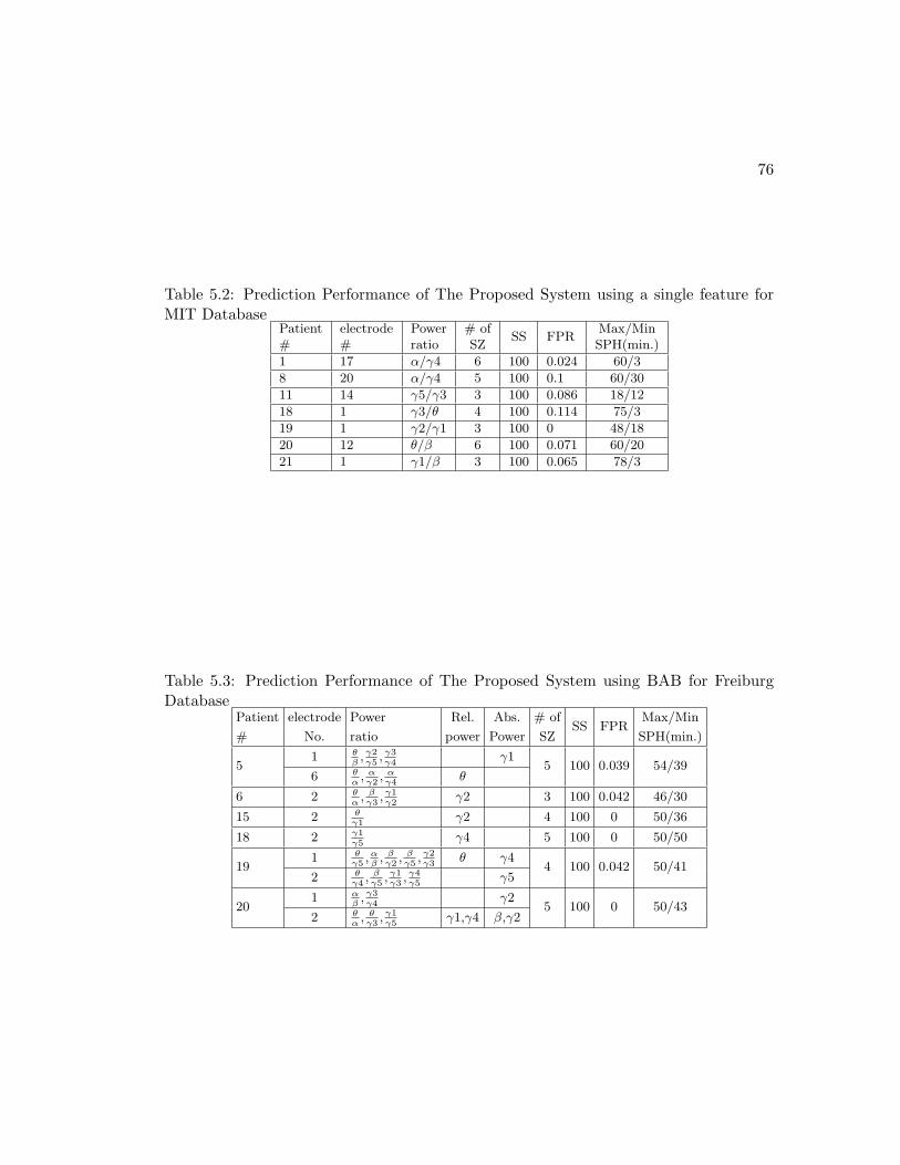
76
Table 5.2: Prediction Performance of The Proposed System using a single feature forMIT Database
Patient electrode Power # ofSS FPR
Max/Min# # ratio SZ SPH(min.)
1 17 α/γ4 6 100 0.024 60/3
8 20 α/γ4 5 100 0.1 60/30
11 14 γ5/γ3 3 100 0.086 18/12
18 1 γ3/θ 4 100 0.114 75/3
19 1 γ2/γ1 3 100 0 48/18
20 12 θ/β 6 100 0.071 60/20
21 1 γ1/β 3 100 0.065 78/3
Table 5.3: Prediction Performance of The Proposed System using BAB for FreiburgDatabase
Patient electrode Power Rel. Abs. # ofSS FPR
Max/Min
# No. ratio power Power SZ SPH(min.)
51 θ
β, γ2γ5
, γ3γ4
γ15 100 0.039 54/39
6 θα, αγ2
, αγ4
θ
6 2 θα, βγ3
, γ1γ2
γ2 3 100 0.042 46/30
15 2 θγ1
γ2 4 100 0 50/36
18 2 γ1γ5
γ4 5 100 0 50/50
191 θ
γ5,αβ, βγ2
, βγ5
, γ2γ3
θ γ44 100 0.042 50/41
2 θγ4
, βγ5
, γ1γ3
, γ4γ5
γ5
201 α
β, γ3γ4
γ25 100 0 50/43
2 θα, θγ3
, γ1γ5
γ1,γ4 β,γ2

77
Table 5.4: Prediction Performance of The Proposed System using BAB for MITDatabase
Patient electrode Power Rel. Abs. # ofSS FPR
Max/Min
# No. ratio power Power SZ SPH(min.)
2 18 γ1γ4
, γ2γ5
θ,α 3 100 0.029 60/39
37 β
γ2, γ1γ4
, γ3γ4
θ γ45 100 0 68/15
8 γ1γ4
, γ2γ3
γ2
5 8 θα, θγ2
, θγ3
, βγ1
, βγ4
, γ4γ5
θ,γ2 5 100 0.051 60/10
68 γ1
γ2, γ3γ4
γ26 83.3 0.045 72/21
21 αβ, αγ5
, γ2γ3
, γ4γ5
γ1,γ5
912 θ
γ3,αβ, γ1γ5
, γ2γ4
γ43 100 0.046 69/33
18 γ1γ3
, γ2γ4
α
101 β
γ3, γ3γ4
, γ3γ5
γ2 α,γ27 100 0.060 69/24
18 θγ4
,αβ, αγ2
γ5 θ,γ3
131 γ1
γ2, γ3γ4
γ2,γ5 θ6 100 0.030 68/18
18 γ1γ2
, γ3γ4
γ2,γ5 θ
14 14 θα, θγ4
, γ3γ4
, γ4γ5
θ β,γ2 5 100 0.039 60/6
16 27 βγ3
, γ1γ4
, γ1γ5
, γ2γ5
θ 3 100 0 58/42
22 11 θγ3
, βγ2
, γ1γ5
, γ2γ4
, γ3γ5
θ 3 100 0.032 78/11
database and for the remaining 10 patients in MIT database are shown in Table 5.3 and
in Table 5.4, respectively. Details about the spectral power ratios, relative spectral
powers, absolute spectral powers used for prediction are shown in the 3rd, 4th and 5th
columns, respectively.
Summary of the overall prediction performance for both databases is shown in Table
5.5. For Freiburg intra-cranial EEG database, the proposed algorithm achieved a sensi-
tivity of 100% and a FPR of 0.032 using 1.167 electrodes and 2.78 features on average.
For MIT scalp EEG database, the proposed algorithm achieved a sensitivity of 98.68%
and a FPR of 0.0465 using 1.29 electrodes and 5.05 features on average. Table 5.6
Table 5.5: Overall Prediction Performance of The Proposed System for Freiburg andMIT Databses
DatabaseEEG Mean # of Mean# of
SS FPRtype electrodes features
Freiburg iEEG 1.167 2.78 100 0.0324MIT sEEG 1.294 5.05 98.68 0.0465
and Table 5.7 compare the prediction performance between LASSO and BAB for the
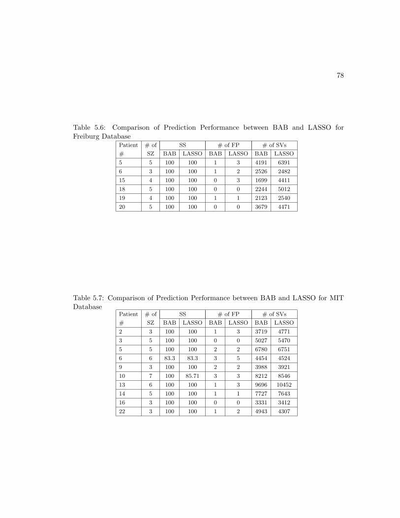
78
Table 5.6: Comparison of Prediction Performance between BAB and LASSO forFreiburg Database
Patient # of SS # of FP # of SVs
# SZ BAB LASSO BAB LASSO BAB LASSO
5 5 100 100 1 3 4191 6391
6 3 100 100 1 2 2526 2482
15 4 100 100 0 3 1699 4411
18 5 100 100 0 0 2244 5012
19 4 100 100 1 1 2123 2540
20 5 100 100 0 0 3679 4471
Table 5.7: Comparison of Prediction Performance between BAB and LASSO for MITDatabase
Patient # of SS # of FP # of SVs
# SZ BAB LASSO BAB LASSO BAB LASSO
2 3 100 100 1 3 3719 4771
3 5 100 100 0 0 5027 5470
5 5 100 100 2 2 6780 6751
6 6 83.3 83.3 3 5 4454 4524
9 3 100 100 2 2 3988 3921
10 7 100 85.71 3 3 8212 8546
13 6 100 100 1 3 9696 10452
14 5 100 100 1 1 7727 7643
16 3 100 100 0 0 3331 3412
22 3 100 100 1 2 4943 4307
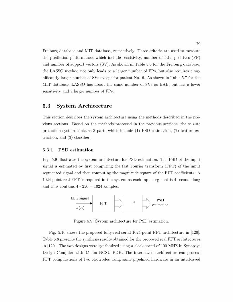
79
Freiburg database and MIT database, respectively. Three criteria are used to measure
the prediction performance, which include sensitivity, number of false positives (FP)
and number of support vectors (SV). As shown in Table 5.6 for the Freiburg database,
the LASSO method not only leads to a larger number of FPs, but also requires a sig-
nificantly larger number of SVs except for patient No. 6. As shown in Table 5.7 for the
MIT database, LASSO has about the same number of SVs as BAB, but has a lower
sensitivity and a larger number of FPs.
5.3 System Architecture
This section describes the system architecture using the methods described in the pre-
vious sections. Based on the methods proposed in the previous sections, the seizure
prediction system contains 3 parts which include (1) PSD estimation, (2) feature ex-
traction, and (3) classifier.
5.3.1 PSD estimation
Fig. 5.9 illustrates the system architecture for PSD estimation. The PSD of the input
signal is estimated by first computing the fast Fourier transform (FFT) of the input
segmented signal and then computing the magnitude square of the FFT coefficients. A
1024-point real FFT is required in the system as each input segment is 4 seconds long
and thus contains 4 ∗ 256 = 1024 samples.
EEG signal
FFT |·|2PSD
estimation
Figure 5.9: System architecture for PSD estimation.
Fig. 5.10 shows the proposed fully-real serial 1024-point FFT architecture in [120].
Table 5.8 presents the synthesis results obtained for the proposed real FFT architectures
in [120]. The two designs were synthesized using a clock speed of 100 MHZ in Synopsys
Design Compiler with 45 nm NCSU PDK. The interleaved architecture can process
FFT computations of two electrodes using same pipelined hardware in an interleaved
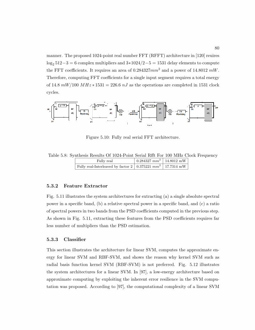
80
manner. The proposed 1024-point real number FFT (RFFT) architecture in [120] reuires
log2 512−3 = 6 complex multipliers and 3∗1024/2−5 = 1531 delay elements to compute
the FFT coefficients. It requires an area of 0.284327mm2 and a power of 14.8012 mW .
Therefore, computing FFT coefficients for a single input segment requires a total energy
of 14.8 mW/100 MHz ∗ 1531 = 226.6 nJ as the operations are completed in 1531 clock
cycles.
Figure 5.10: Fully real serial FFT architecture.
Table 5.8: Synthesis Results Of 1024-Point Serial Rfft For 100 MHz Clock FrequencyFully real 0.284327 mm2 14.8012 mW
Fully real-Interleaved by factor 2 0.375221 mm2 17.7314 mW
5.3.2 Feature Extractor
Fig. 5.11 illustrates the system architectures for extracting (a) a single absolute spectral
power in a specific band, (b) a relative spectral power in a specific band, and (c) a ratio
of spectral powers in two bands from the PSD coefficients computed in the previous step.
As shown in Fig. 5.11, extracting these features from the PSD coefficients requires far
less number of multipliers than the PSD estimation.
5.3.3 Classifier
This section illustrates the architecture for linear SVM, computes the approximate en-
ergy for linear SVM and RBF-SVM, and shows the reason why kernel SVM such as
radial basis function kernel SVM (RBF-SVM) is not preferred. Fig. 5.12 illustrates
the system architectures for a linear SVM. In [97], a low-energy architecture based on
approximate computing by exploiting the inherent error resilience in the SVM compu-
tation was proposed. According to [97], the computational complexity of a linear SVM

81
Retain coefficients
in band 1
PSD
estimationAccumulator Log
Absolute
spectral
power
(a)
Relative
spectral
power
Retain coefficients
in band 1
Retain coefficients
in total band
PSD
estimation
PSD
estimation
Accumulator
Accumulator
Log
Log
-
(b)
Ratio of
spectral
powers
Retain coefficients
in band 1
Retain coefficients
in band 2
PSD
estimation
PSD
estimation
Accumulator
Accumulator
Log
Log
-
(c)
Figure 5.11: System architectures for extracting (a) a single absolute spectral in aspecific band, (b) a relative spectral power in a specific band, and (c) a ratio of spectralpowers in two bands from the PSD coefficients.
only depends on the feature dimension. However, the computational complexity of a
RBF-SVM consists of 2 parts, which include kernel computation and decision variable
computation. The computational complexity of a RBF-SVM classifier is not only pro-
portional to the feature dimension, but also to the number of support vectors (SVs).
Table 5.9 compares the number of support vectors after training using linear SVM and
RBF-SVM for Patient No. 10 and Patient No. 13 in the MIT database. The fourth
and fifth columns of Table 5.9 show the approximate estimates of the energy in kernel
computation and decision variable computation per test vector using the results in [97].
The last column shows the total energy per test vector. As shown in the table, even
though RBF-SVM requires significantly less number of SVs than the linear SVM, its
energy requirement is 3 orders of magnitude larger than the linear SVM.
Thus, regardless of the energy required in sensors and analog-to-digital converters
(ADC), the total energy required in feature extraction and classification using a single
electrode is approximately 227 nJ when linear SVM is used. That number is increased
to 2∗227 = 454 nJ for Patient No. 10 and for Patient No. 13 in the MIT database as the

82
Feature 1
f1(l)
Feature 2
f2(l)
Feature r
fr(l)
w1
w2
wr
b
Sign
+1
0
l
Output
y(l)
Figure 5.12: System architecture for linear SVM.
interleaved architecture requires twice the number of clock cycles for feature extraction.
When RBF-SVM is used, the energy consumption increases to 586 nJ and 490 nJ per
test vector for Patient No. 10 and for Patient No. 13 in the MIT database, respectively.
These energy consumption estimates are obtained by interpolating the energy estimates
in [97, 120]. The energy consumption of the Kalman filter is not included in this analysis.
The RBF-SVM not only requires more energy consumption, it also requires additional
hardware for approximately 23900 multiplications and 1992 RBF kernel computations
for Patient No. 10, and for 6000 multiplications and 585 RBF kernel computations for
Patient No. 13. The number of multiplications increases by a factor of Nsv for RBF-
SVM, where Nsv represents the number of support vectors. Furthermore, Nsv additional
kernel evaluation are needed in the RBF-SVM.
Table 5.9: Comparison of Energy Consumption between Linear SVM and RBF-SVMfor MIT Database.Patient # of # of SVs kernel decision variable classifier energy total energy
# features SVMRBF-SVM SVMRBF-SVM SVM RBF-SVM SVM RBF-SVM SVM RBF-SVM
10 12 8212 1992 – 108 nJ 32 pJ 24 nJ 32 pJ 132 nJ 454 nJ 586 nJ
13 10 9696 585 – 30 nJ 30 pJ 6 nJ 30 pJ 36 nJ 454 nJ 490 nJ
5.4 Discussion
Many approaches have been presented for predicting seizures in epileptic patients. Var-
ious types of linear and nonlinear features have been used for seizure prediction. Our

83
Table 5.10: Comparison to prior work
Reference EEG Sensi- FPR Feature No. of
type tivity Type features
Chisci et al. 2010 iEEG 100 0.17 AR coeff. 36
Wang et al. 2014 iEEG 98.80 0.054Amplitude and Frequency 125
Park et al. 2011 iEEG 97.5 0.27 PSD 36
Ozdemir et al. 2014 iEEG 96.55 0.21 Hilbert Spectrum 14.49
Ayinala et al. 2012 iEEG 94.37 0.14 PSD 4.8
Aarabi et al. 2014 iEEG 92.60 0.15 Model parameters 72
Williamson et al. 2011 iEEG 90.8 0.095 correlation 36
Aschenbrenner et al. 2003 iEEG 84.2 1.0 correlation 25
Zheng et al. 2013 iEEG 80 0.17 Phase Coherence 3
Maiwald et al. 2004 iEEG 41.5 0.15 correlation 25
Bandarabadi et al. 2014 iEEG 75.8 0.1 PSD 9.9
Alexandre et al. 2014 iEEG 50 0.15 Various 22
Khammari et al. 2012 sEEG 85 – PSD 30
proposediEEG 100 0.032 PSD ratio 2.78
iEEG
proposedsEEG 98.68 0.047 PSD ratio 5.05
sEEG

84
results are compared directly to several other studies that have tested prediction algo-
rithms using the same Freiburg EEG database [121, 50, 22, 94, 122, 123, 124, 52, 125,
126] or MIT EEG database [127]. Our results may also be compared to studies using
other databases [51, 28]. We demonstrate high sensitivity, low FPR, and low feature
dimension for these two databases.
Table 5.10 compares the system performance of the proposed algorithm with prior
works. The proposed algorithm for seizure prediction, using the least number of features
selected by the BAB algorithm (for iEEG), achieves the highest sensitivity (for iEEG)
and the lowest FPR.
Even though the proposed algorithm has been tested on short duration EEG data,
future work will be directed towards analysis on long term EEG recordings.
Another evaluation criterion, successful patient rate, was proposed in [128] and is
used to evaluate the success of a seizure prediction algorithm. A patient is considered
as a successful patient if the sensitivity is 100% and the FP rate is lower than 0.2. We
achieved a FPR of 0 for 10 out of 19 patients in the Freiburg database and for 3 out of
17 patients for the MIT database. We also achieved a successful patient rate of 100%
for the Freiburg database and a successful patient rate of 94.1% for the MIT database.
System performance is degraded for the scalp EEG recordings as the MIT (sEEG)
database has a lower sensitivity, a lower successful patient rate, and a higher FP rate
than the Freiburg (iEEG) database. This is caused by the fact that intracranial EEG
recordings usually have a higher spatial resolution and signal-to-noise ratio due to
greater proximity to neural activity. Therefore, sEEG is a much noisier measurement
of the neural activity and is highly suspectable to the interferences from the outer en-
vironment than the iEEG, which leads to the decrease of sensitivity and the increase
of FP rate. However, since iEEG is an invasive signal, the process to obtain invasive
EEG recordings brings the risk of infections. Furthermore, the patient’s hospital stay
for surgery to implant these electrodes can be expensive. In addition, the sEEG has a
larger coverage of the brain than iEEG.
In addition, the proposed seizure prediction algorithm using BAB for feature selec-
tion has several advantages over using LASSO for feature selection. The BAB algorithm
achieves a higher sensitivity and a lower FPR for both databases. The BAB algorithm
also requires a smaller number of SVs than LASSO on the Freiburg database.

85
Finally, the total energy consumption of the system using linear SVM is reduced by
8% to 23% compared to system using RBF-SVM. In analysis of long-term EEG data,
number of support vectors will increase proportionally to the number of total feature
vectors. Thus, the energy consumption of a RBF-SVM will be greatly increased when
long-term EEG is analyzed, and the reduction in total energy consumption of the system
using linear SVM will be greatly increased compared to the system using RBF-SVM.
5.5 Conclusion
In this chapter, a patient-specific algorithm for seizure prediction using unipolar or
bipolar EEG signals from either one or two channels has been proposed. This algorithm
achieves a sensitivity of 100%, a successful patient rate of 100% a FP rate of 0.032 per
hour on average for iEEG recordings, and achieves a sensitivity of 98.68%, a successful
patient rate of 94.1% and a FP rate of 0.047 per hour on average for iEEG recordings.
Compared with the results in [121, 50, 22, 94, 122, 123, 124, 52, 125, 126, 127], the
proposed algorithm uses the fewest number of features and achieves a high sensitivity
and a lower FP rate. The proposed approach reduces the complexity and area by about
2 to 3 orders of magnitude. We conclude that using discriminative sparse important
features and using a simple classifier such as linear SVM can lead to higher sensitivity
and specificity compared to processing hundreds of features with a complex classifier
such as RBF-SVM.
Many algorithms that work well on short EEG recordings (like one day) fail to work
on longer recordings (i.e., several days to weeks). Future work will be directed towards
validating the proposed approach on longer term recordings. The spectral powers in
eight subbands are sufficient for signals sampled at 256 Hz. However, further research
needs to be directed to find out how many subbands are sufficient for high-frequency
recordings such as 1 kHz or 2 kHz.
Chapter 6
Seizure Prediction from
Long-Term Fragmented EEG
Recordings
In the proposed approach [81, 96], we first extract two sets of features. A window based
feature extraction is used, where the window size is 4 second for spectral feature set
and is 10 second for the correlation feature set, respectively. The 10-second window for
correlation is chosen for an accurate estimate of the correlation coefficient. The first
feature set includes spectral powers and spectral ratios. The second feature set includes
correlation coefficients between all possible pairs of electrodes. The two feature sets are
then subjected to feature selection and classification independently. Three classifiers are
used and tested on the selected features, which include AdaBoost, radial basis function
kernel support vector machine (RBF-SVM), and artificial neural netwroks (ANN).
6.1 Patients Database
We consider the dataset from the recent American Epilepsy Society Seizure Prediction
Challenge database [129]. The experimental procedures involving human subjects were
approved by the Institutional Review Board. The Institutions Ethical Review Board
86
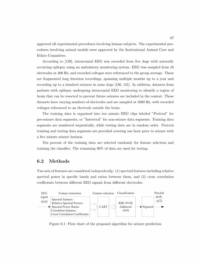
87
approved all experimental procedures involving human subjects. The experimental pro-
cedures involving animal models were approved by the Institutional Animal Care and
Ethics Committee.
According to [129], intracranial EEG was recorded from five dogs with naturally
occurring epilepsy using an ambulatory monitoring system. EEG was sampled from 16
electrodes at 400 Hz, and recorded voltages were referenced to the group average. These
are fragmented long duration recordings, spanning multiple months up to a year and
recording up to a hundred seizures in some dogs [130, 131]. In addition, datasets from
patients with epilepsy undergoing intracranial EEG monitoring to identify a region of
brain that can be resected to prevent future seizures are included in the contest. These
datasets have varying numbers of electrodes and are sampled at 5000 Hz, with recorded
voltages referenced to an electrode outside the brain.
The training data is organized into ten minute EEG clips labeled ”Preictal” for
pre-seizure data segments, or ”Interictal” for non-seizure data segments. Training data
segments are numbered sequentially, while testing data are in random order. Preictal
training and testing data segments are provided covering one hour prior to seizure with
a five minute seizure horizon.
Ten percent of the training data are selected randomly for feature selection and
training the classifier. The remaining 90% of data are used for testing.
6.2 Methods
Two sets of features are considered independently : (1) spectral features including relative
spectral power in specific bands and ratios between them, and (2) cross correlation
coefficients between different EEG signals from different electrodes.
Feature extraction
)(nsSpectral features:
Relative Spectral Powers
Spectral Power Ratios
Correlation features:
Cross Correlation Coefficients
CART
Feature selection
RBF-SVM/
Adaboost/
ANN
Classification
Sigmoid
Precital
prob.EEG
signal
Figure 6.1: Flow chart of the proposed algorithm for seizure prediction
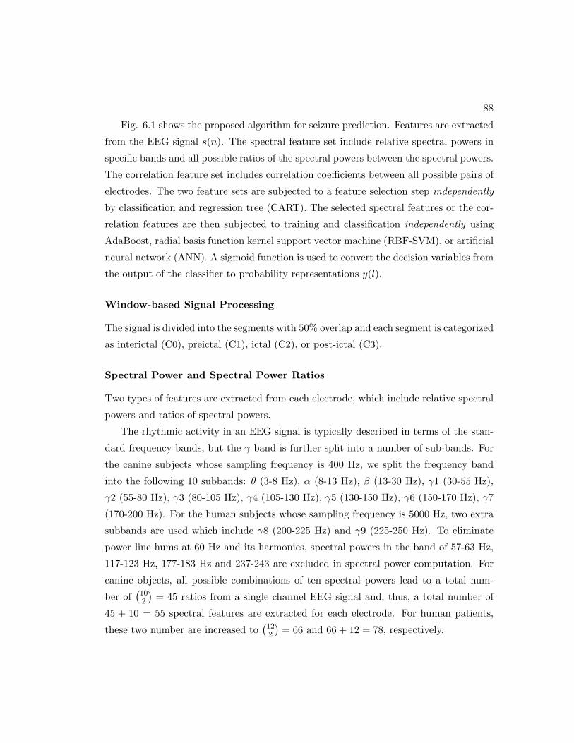
88
Fig. 6.1 shows the proposed algorithm for seizure prediction. Features are extracted
from the EEG signal s(n). The spectral feature set include relative spectral powers in
specific bands and all possible ratios of the spectral powers between the spectral powers.
The correlation feature set includes correlation coefficients between all possible pairs of
electrodes. The two feature sets are subjected to a feature selection step independently
by classification and regression tree (CART). The selected spectral features or the cor-
relation features are then subjected to training and classification independently using
AdaBoost, radial basis function kernel support vector machine (RBF-SVM), or artificial
neural network (ANN). A sigmoid function is used to convert the decision variables from
the output of the classifier to probability representations y(l).
Window-based Signal Processing
The signal is divided into the segments with 50% overlap and each segment is categorized
as interictal (C0), preictal (C1), ictal (C2), or post-ictal (C3).
Spectral Power and Spectral Power Ratios
Two types of features are extracted from each electrode, which include relative spectral
powers and ratios of spectral powers.
The rhythmic activity in an EEG signal is typically described in terms of the stan-
dard frequency bands, but the γ band is further split into a number of sub-bands. For
the canine subjects whose sampling frequency is 400 Hz, we split the frequency band
into the following 10 subbands: θ (3-8 Hz), α (8-13 Hz), β (13-30 Hz), γ1 (30-55 Hz),
γ2 (55-80 Hz), γ3 (80-105 Hz), γ4 (105-130 Hz), γ5 (130-150 Hz), γ6 (150-170 Hz), γ7
(170-200 Hz). For the human subjects whose sampling frequency is 5000 Hz, two extra
subbands are used which include γ8 (200-225 Hz) and γ9 (225-250 Hz). To eliminate
power line hums at 60 Hz and its harmonics, spectral powers in the band of 57-63 Hz,
117-123 Hz, 177-183 Hz and 237-243 are excluded in spectral power computation. For
canine objects, all possible combinations of ten spectral powers lead to a total num-
ber of(102
)= 45 ratios from a single channel EEG signal and, thus, a total number of
45 + 10 = 55 spectral features are extracted for each electrode. For human patients,
these two number are increased to(122
)= 66 and 66 + 12 = 78, respectively.
89
Fig. 6.2 illustrates the normalized (between 0 and 1) relative spectral power in band
[8, 13] Hz (top pannel), the spectral power in band [13, 30] Hz (middle pannel) and
the spectral power ratio of P8,13-to-P13,30 using the EEG recordings in electrode No.
13 of Patient No. 1 from the American Epilepsy Society Seizure Prediction Challenge
database, where the red vertical lines represent the preictal onsets. While the spectral
power features in both bands are indiscriminate of the preictal and interictal periods,
the ratio between them shows strong detectability of the seizures as this ratio increases
significantly after the precital onsets.
0 2 4 6 8 10 120
0.5
1
e13,
Q8,1
3
0 2 4 6 8 10 120
0.5
1
e13,
Q13,2
0
0 2 4 6 8 10 120
0.5
1
hour
e13,
P8,1
3/P
13,2
0
Figure 6.2: Spectral power in in band [8, 13] Hz (top pannel), spectral power in band[13, 30] Hz (middle pannel) and the spectral power ratio of P8,13-to-P13,30 using the EEGrecordings in electrode No. 13 of Patient No. 1 from the American Epilepsy SocietySeizure Prediction Challenge database.
Cross-correlation coefficients
Cross-correlation coefficients between all pairs of electrodes are extracted as another
feature set. Fig. 6.3 illustrates the cross correlation coefficient between electrode No.
1 and electrode No. 10 using the EEG recordings of Patient No. 2 from the American
Epilepsy Society Seizure Prediction Challenge database, where the red vertical line
represents the preictal onsets. The similarity between these 2 electrodes shows strong
predictability of the seizures as this coefficient increases after the precital onsets.
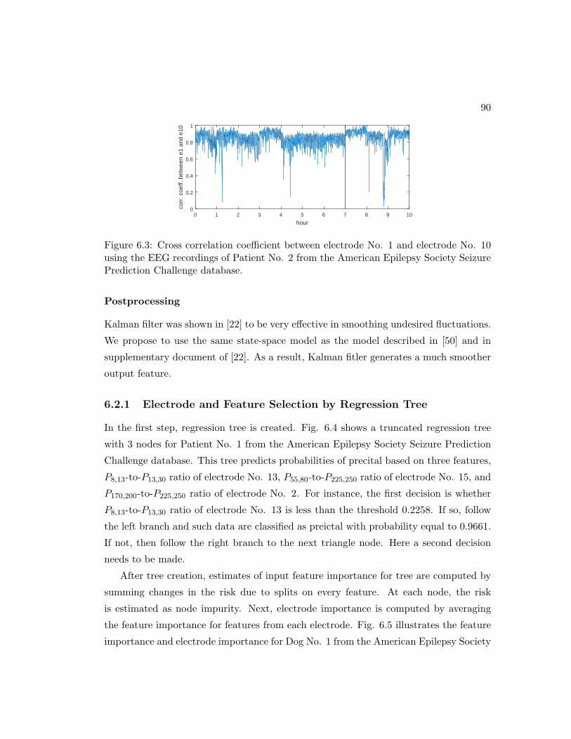
90
hour0 1 2 3 4 5 6 7 8 9 10
corr
. coe
ff. b
etw
een
e1 a
nd e
10
0
0.2
0.4
0.6
0.8
1
Figure 6.3: Cross correlation coefficient between electrode No. 1 and electrode No. 10using the EEG recordings of Patient No. 2 from the American Epilepsy Society SeizurePrediction Challenge database.
Postprocessing
Kalman filter was shown in [22] to be very effective in smoothing undesired fluctuations.
We propose to use the same state-space model as the model described in [50] and in
supplementary document of [22]. As a result, Kalman fitler generates a much smoother
output feature.
6.2.1 Electrode and Feature Selection by Regression Tree
In the first step, regression tree is created. Fig. 6.4 shows a truncated regression tree
with 3 nodes for Patient No. 1 from the American Epilepsy Society Seizure Prediction
Challenge database. This tree predicts probabilities of precital based on three features,
P8,13-to-P13,30 ratio of electrode No. 13, P55,80-to-P225,250 ratio of electrode No. 15, and
P170,200-to-P225,250 ratio of electrode No. 2. For instance, the first decision is whether
P8,13-to-P13,30 ratio of electrode No. 13 is less than the threshold 0.2258. If so, follow
the left branch and such data are classified as preictal with probability equal to 0.9661.
If not, then follow the right branch to the next triangle node. Here a second decision
needs to be made.
After tree creation, estimates of input feature importance for tree are computed by
summing changes in the risk due to splits on every feature. At each node, the risk
is estimated as node impurity. Next, electrode importance is computed by averaging
the feature importance for features from each electrode. Fig. 6.5 illustrates the feature
importance and electrode importance for Dog No. 1 from the American Epilepsy Society
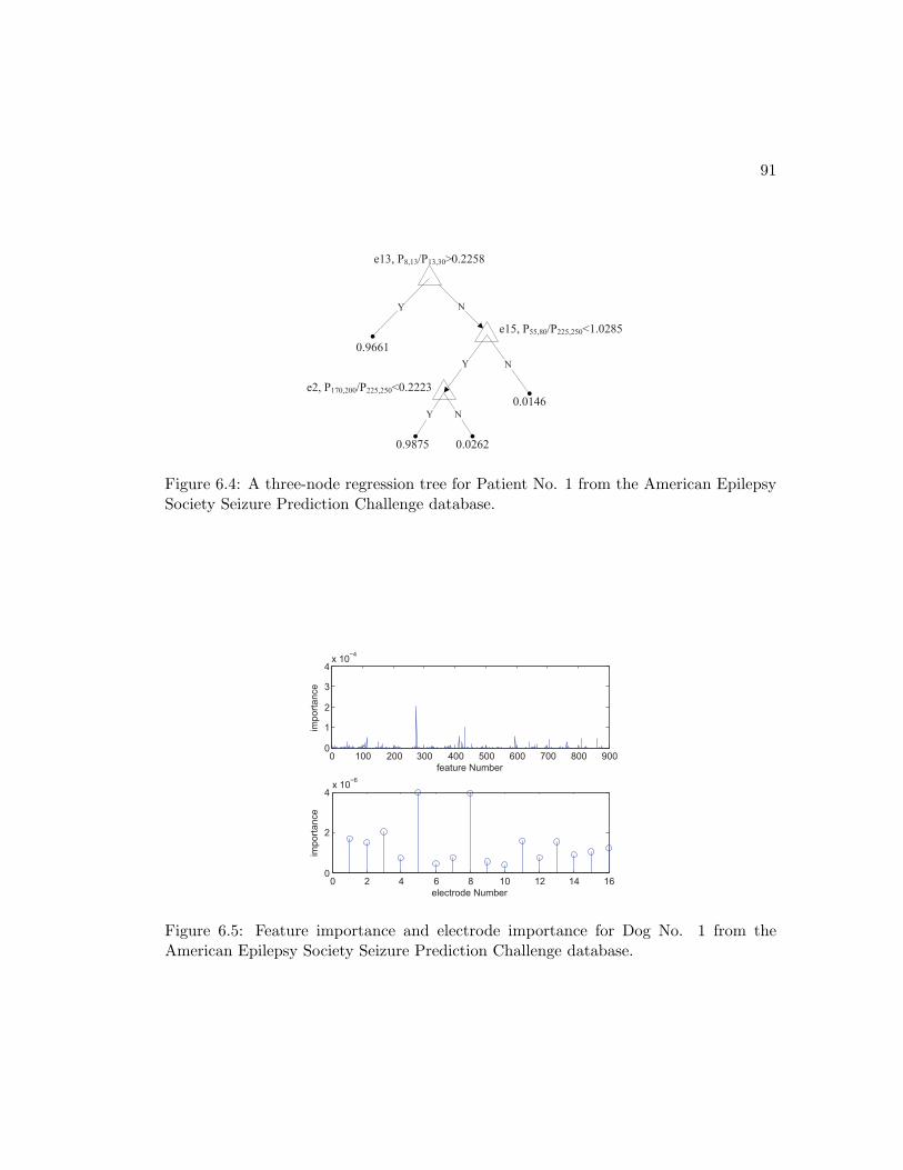
91
N
Y
Y
Y
N
N
0.9661
0.9875 0.0262
0.0146
e13, P8,13/P13,30
e15, P55,80/P225,250<1.0285
e2, P170,200/P225,250<0.2223
> 0.2258
Figure 6.4: A three-node regression tree for Patient No. 1 from the American EpilepsySociety Seizure Prediction Challenge database.
0 100 200 300 400 500 600 700 800 9000
1
2
3
4x 10
−4
feature Number
import
ance
0 2 4 6 8 10 12 14 160
2
4x 10
−6
electrode Number
import
ance
Figure 6.5: Feature importance and electrode importance for Dog No. 1 from theAmerican Epilepsy Society Seizure Prediction Challenge database.

92
Seizure Prediction Challenge database. As shown in Fig. 6.5, five most important
electrodes for classification include electrode No. 1, 3, 5, 8 and 11.
After electrode selection, feature selection is further performed on the features from
the selected electrodes using CART. Features are then sorted according to their im-
portance in the tree and the most important features are selected. For instance, the
most important electrodes for Dog No. 1 from the American Epilepsy Society Seizure
Prediction Challenge database include electrode No. 1, 3, 5, 8, and 11. A total of
5 ∗ 55 = 275 features can be extracted from these 5 electrodes. After tree creation
on these 275 features, importance for each feature is estimated. Fig. 6.6 shows the
sorted feature importance for Dog No. 1 in a descending order, where the 50th most
important feature is less than 2% of the most important feature. As a result, 50 most
important features are selected and features whose importance are less than 2% of the
most important one are discarded.
0 50 100 150 200 250 3000
1
2
3x 10
−4
featu
re im
port
ance
sorted feature index
Figure 6.6: Sorted feature importance for Dog No. 1 from the American EpilepsySociety Seizure Prediction Challenge database in a descending order.
6.2.2 Seizure Prediction Classification
AdaBoost, polynomial SVM with degree of 2, radial basis function kernel SVM (RBF-
SVM), and artificial neural networks (ANNs) are used for classification and their per-
formance characteristics are compared.
After computing the decision variable, a sigmoid function, S(p(t − c)), is used to
convert its values into probabilities, where c represents the center of the function and
p represents spread of the function, respectively. Fig. 6.7 illustrates the input decision
variable and output seizure probability of the sigmoid function.
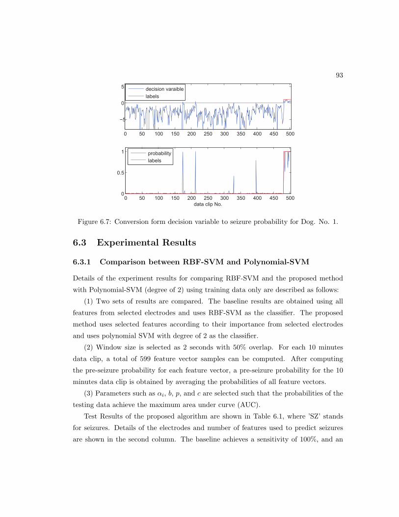
93
0 50 100 150 200 250 300 350 400 450 500
−5
0
5 decision varaible
labels
0 50 100 150 200 250 300 350 400 450 5000
0.5
1
data clip No.
probability
labels
Figure 6.7: Conversion form decision variable to seizure probability for Dog. No. 1.
6.3 Experimental Results
6.3.1 Comparison between RBF-SVM and Polynomial-SVM
Details of the experiment results for comparing RBF-SVM and the proposed method
with Polynomial-SVM (degree of 2) using training data only are described as follows:
(1) Two sets of results are compared. The baseline results are obtained using all
features from selected electrodes and uses RBF-SVM as the classifier. The proposed
method uses selected features according to their importance from selected electrodes
and uses polynomial SVM with degree of 2 as the classifier.
(2) Window size is selected as 2 seconds with 50% overlap. For each 10 minutes
data clip, a total of 599 feature vector samples can be computed. After computing
the pre-seizure probability for each feature vector, a pre-seizure probability for the 10
minutes data clip is obtained by averaging the probabilities of all feature vectors.
(3) Parameters such as αi, b, p, and c are selected such that the probabilities of the
testing data achieve the maximum area under curve (AUC).
Test Results of the proposed algorithm are shown in Table 6.1, where ’SZ’ stands
for seizures. Details of the electrodes and number of features used to predict seizures
are shown in the second column. The baseline achieves a sensitivity of 100%, and an
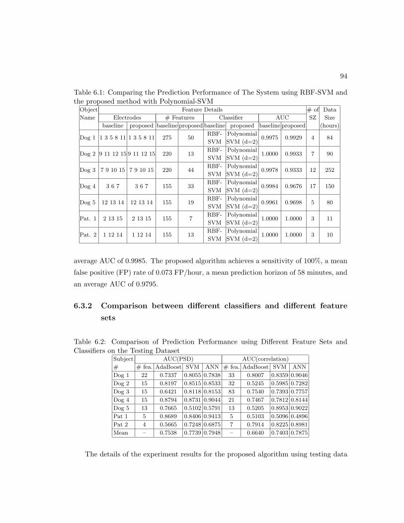
94
Table 6.1: Comparing the Prediction Performance of The System using RBF-SVM andthe proposed method with Polynomial-SVMObject Feature Details # of Data
Name Electrodes # Features Classifier AUC SZ Size
baseline proposed baseline proposed baseline proposed baseline proposed (hours)
Dog 1 1 3 5 8 11 1 3 5 8 11 275 50RBF- Polynomial
0.9975 0.9929 4 84SVM SVM (d=2)
Dog 2 9 11 12 15 9 11 12 15 220 13RBF- Polynomial
1.0000 0.9933 7 90SVM SVM (d=2)
Dog 3 7 9 10 15 7 9 10 15 220 44RBF- Polynomial
0.9978 0.9333 12 252SVM SVM (d=2)
Dog 4 3 6 7 3 6 7 155 33RBF- Polynomial
0.9984 0.9676 17 150SVM SVM (d=2)
Dog 5 12 13 14 12 13 14 155 19RBF- Polynomial
0.9961 0.9698 5 80SVM SVM (d=2)
Pat. 1 2 13 15 2 13 15 155 7RBF- Polynomial
1.0000 1.0000 3 11SVM SVM (d=2)
Pat. 2 1 12 14 1 12 14 155 13RBF- Polynomial
1.0000 1.0000 3 10SVM SVM (d=2)
average AUC of 0.9985. The proposed algorithm achieves a sensitivity of 100%, a mean
false positive (FP) rate of 0.073 FP/hour, a mean prediction horizon of 58 minutes, and
an average AUC of 0.9795.
6.3.2 Comparison between different classifiers and different feature
sets
Table 6.2: Comparison of Prediction Performance using Different Feature Sets andClassifiers on the Testing Dataset
Subject AUC(PSD) AUC(correlation)
# # fea. AdaBoost SVM ANN # fea. AdaBoost SVM ANN
Dog 1 22 0.7337 0.8055 0.7838 33 0.8007 0.8359 0.9046
Dog 2 15 0.8197 0.8515 0.8533 32 0.5245 0.5985 0.7282
Dog 3 15 0.6421 0.8118 0.8153 83 0.7540 0.7393 0.7757
Dog 4 15 0.8794 0.8731 0.9044 21 0.7467 0.7812 0.8144
Dog 5 13 0.7665 0.5102 0.5791 13 0.5205 0.8953 0.9022
Pat 1 5 0.8689 0.8406 0.9413 5 0.5103 0.5096 0.4896
Pat 2 4 0.5665 0.7248 0.6875 7 0.7914 0.8225 0.8981
Mean – 0.7538 0.7739 0.7948 – 0.6640 0.7403 0.7875
The details of the experiment results for the proposed algorithm using testing data
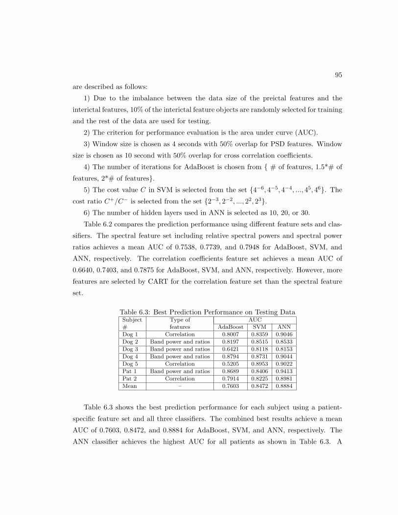
95
are described as follows:
1) Due to the imbalance between the data size of the preictal features and the
interictal features, 10% of the interictal feature objects are randomly selected for training
and the rest of the data are used for testing.
2) The criterion for performance evaluation is the area under curve (AUC).
3) Window size is chosen as 4 seconds with 50% overlap for PSD features. Window
size is chosen as 10 second with 50% overlap for cross correlation coefficients.
4) The number of iterations for AdaBoost is chosen from { # of features, 1.5*# of
features, 2*# of features}.5) The cost value C in SVM is selected from the set {4−6, 4−5, 4−4, ..., 45, 46}. The
cost ratio C+/C− is selected from the set {2−3, 2−2, ..., 22, 23}.6) The number of hidden layers used in ANN is selected as 10, 20, or 30.
Table 6.2 compares the prediction performance using different feature sets and clas-
sifiers. The spectral feature set including relative spectral powers and spectral power
ratios achieves a mean AUC of 0.7538, 0.7739, and 0.7948 for AdaBoost, SVM, and
ANN, respectively. The correlation coefficients feature set achieves a mean AUC of
0.6640, 0.7403, and 0.7875 for AdaBoost, SVM, and ANN, respectively. However, more
features are selected by CART for the correlation feature set than the spectral feature
set.
Table 6.3: Best Prediction Performance on Testing DataSubject Type of AUC# features AdaBoost SVM ANN
Dog 1 Correlation 0.8007 0.8359 0.9046
Dog 2 Band power and ratios 0.8197 0.8515 0.8533
Dog 3 Band power and ratios 0.6421 0.8118 0.8153
Dog 4 Band power and ratios 0.8794 0.8731 0.9044
Dog 5 Correlation 0.5205 0.8953 0.9022
Pat 1 Band power and ratios 0.8689 0.8406 0.9413
Pat 2 Correlation 0.7914 0.8225 0.8981
Mean – 0.7603 0.8472 0.8884
Table 6.3 shows the best prediction performance for each subject using a patient-
specific feature set and all three classifiers. The combined best results achieve a mean
AUC of 0.7603, 0.8472, and 0.8884 for AdaBoost, SVM, and ANN, respectively. The
ANN classifier achieves the highest AUC for all patients as shown in Table 6.3. A

96
stochastic logic implementation of the ANN classifiers has been presented in [132].
6.4 Conclusion
A patient-specific algorithm for seizure prediction using a small number of EEG signals
has been proposed. The baseline experiment using a large number of features and
RBF-SVM achieves a 100% sensitivity and an average AUC of 0.9985. The proposed
algorithm using only a small number of features and polynomial SVM with degree of 2
achieves a 100% sensitivity, a mean false positive (FP) rate of 0.073 FP/hour, a mean
prediction horizon of 58 minutes, and an average AUC of 0.9795. Therefore, combining
the PSD features and then carefully selecting a small number of these features from a
few electrodes can improve the prediction performance.
Using the testing data provided by the Mayo clinic, it is also shown that the spectral
feature set achieves a mean AUC of 0.7538, 0.7739, and 0.7948 for AdaBoost, SVM,
and ANN, respectively. The correlation coefficients feature set achieves a mean AUC of
0.6640, 0.7403, and 0.7875 for AdaBoost, SVM, and ANN, respectively. The combined
best results which use patient-specific feature sets achieve a mean AUC of 0.7603, 0.8472,
and 0.8884 for AdaBoost, SVM, and ANN, respectively.

Part II
Feature Selection
97

Chapter 7
MUSE: Minimum Uncertainty
and Sample Elimination Based
Binary Feature Selection
A new feature selection algorithm based on minimum uncertainty and sample elimi-
nation (referred as MUSE) is proposed [98]. The three-step algorithm first quantizes
features into bins, ranks the features based on an uncertainty score, selects the feature
with the lowest uncertainty score, and then discards samples based on an impurity met-
ric. The uncertainty score and the impurity metric are defined in Section 7.1.2 and
Section 7.1.3, respectively. The discarded samples are not used for selection of sub-
sequent features. The process is repeated until a stopping criterion is satisfied. The
sample elimination process reduces redundancy and the selection of a feature with the
least uncertainty score increases relevance. These steps are new to the proposed algo-
rithm. The discarding of the samples and the selection of the feature are both nonlinear
operations and are ideal for general machine learning applications where feature samples
may not necessarily be linearly separable.
98
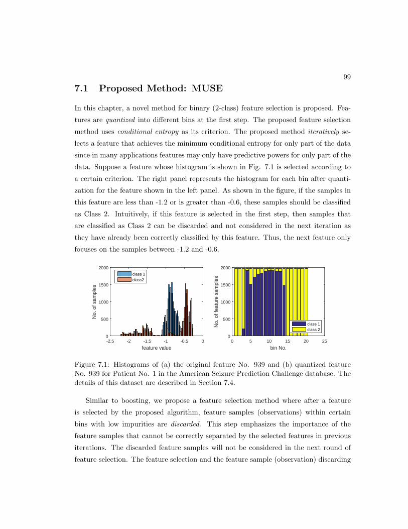
99
7.1 Proposed Method: MUSE
In this chapter, a novel method for binary (2-class) feature selection is proposed. Fea-
tures are quantized into different bins at the first step. The proposed feature selection
method uses conditional entropy as its criterion. The proposed method iteratively se-
lects a feature that achieves the minimum conditional entropy for only part of the data
since in many applications features may only have predictive powers for only part of the
data. Suppose a feature whose histogram is shown in Fig. 7.1 is selected according to
a certain criterion. The right panel represents the histogram for each bin after quanti-
zation for the feature shown in the left panel. As shown in the figure, if the samples in
this feature are less than -1.2 or is greater than -0.6, these samples should be classified
as Class 2. Intuitively, if this feature is selected in the first step, then samples that
are classified as Class 2 can be discarded and not considered in the next iteration as
they have already been correctly classified by this feature. Thus, the next feature only
focuses on the samples between -1.2 and -0.6.
feature value-2.5 -2 -1.5 -1 -0.5 0
No.
of s
ampl
es
0
500
1000
1500
2000class 1class2
bin No.0 5 10 15 20 25
No.
of f
eatu
re s
ampl
es
0
500
1000
1500
2000
class 1class 2
Figure 7.1: Histograms of (a) the original feature No. 939 and (b) quantized featureNo. 939 for Patient No. 1 in the American Seizure Prediction Challenge database. Thedetails of this dataset are described in Section 7.4.
Similar to boosting, we propose a feature selection method where after a feature
is selected by the proposed algorithm, feature samples (observations) within certain
bins with low impurities are discarded. This step emphasizes the importance of the
feature samples that cannot be correctly separated by the selected features in previous
iterations. The discarded feature samples will not be considered in the next round of
feature selection. The feature selection and the feature sample (observation) discarding
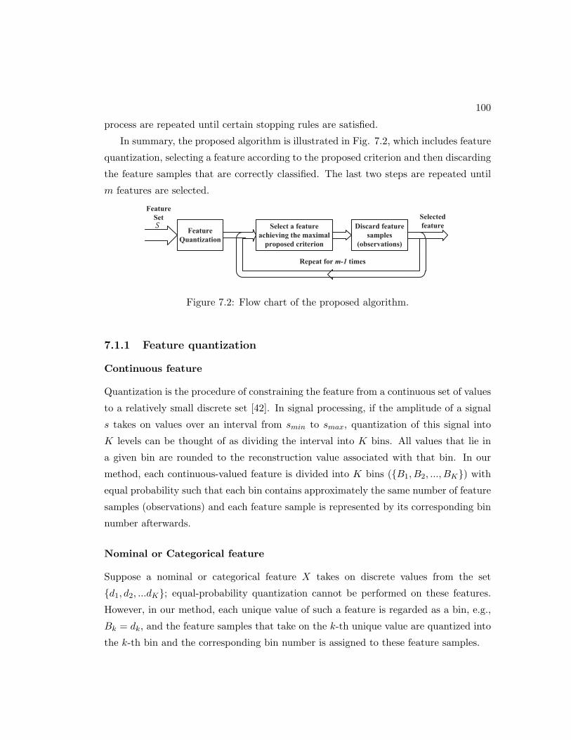
100
process are repeated until certain stopping rules are satisfied.
In summary, the proposed algorithm is illustrated in Fig. 7.2, which includes feature
quantization, selecting a feature according to the proposed criterion and then discarding
the feature samples that are correctly classified. The last two steps are repeated until
m features are selected.
Feature
Set
Feature
Quantization
Select a feature
achieving the maximal
proposed criterion
Selected
featureDiscard feature
samples
(observations)
Repeat for m-1 times
Figure 7.2: Flow chart of the proposed algorithm.
7.1.1 Feature quantization
Continuous feature
Quantization is the procedure of constraining the feature from a continuous set of values
to a relatively small discrete set [42]. In signal processing, if the amplitude of a signal
s takes on values over an interval from smin to smax, quantization of this signal into
K levels can be thought of as dividing the interval into K bins. All values that lie in
a given bin are rounded to the reconstruction value associated with that bin. In our
method, each continuous-valued feature is divided into K bins ({B1, B2, ..., BK}) withequal probability such that each bin contains approximately the same number of feature
samples (observations) and each feature sample is represented by its corresponding bin
number afterwards.
Nominal or Categorical feature
Suppose a nominal or categorical feature X takes on discrete values from the set
{d1, d2, ...dK}; equal-probability quantization cannot be performed on these features.
However, in our method, each unique value of such a feature is regarded as a bin, e.g.,
Bk = dk, and the feature samples that take on the k-th unique value are quantized into
the k-th bin and the corresponding bin number is assigned to these feature samples.

101
7.1.2 Criterion
This section starts with analyzing the criterion used for mRMR and then presents
our new criterion. Since features are quantized first, the new features are discrete
variables. For the purpose of disambiguation, we define S = {X1, ...Xm} as a feature
set with m quantized feature variable (attribute) where X1, ...Xm take particular values
of x1, ...., xm, respectively.
In the first step, the mRMR finds a feature that maximizes the following criterion:
maxXj∈S
[I(Xj ; c)] = H(c)−H(c|Xj) (7.1)
Note that in the first step,∑
i,j I(Xi;Xj) = 0 as no prior feature has been selected.
Let X represent an arbitrary feature and let Bk represent the k-th bin after the first
step of data quantization. Then the mutual information between the class label c and
the feature X can be written as:
I(X; c) = H(c)−∑k
P (Bk)H(c|Bk) (7.2)
where H(c) represents the entropy of the class label and is defined as follows:
H(c) =∑l
−P (cl) logP (cl), (7.3)
cl represents the l-th class label, P (Bk) represents the probability of k-th bin (Bk),
H(c|Bk) represents the conditional entropy of class label given Bk and is defined as
follows:
H(c|Bk) =∑l
−P (cl|Bk) logP (cl|Bk). (7.4)
Since given the class label, H(c) is a fixed number for all features, finding a feature that
maximizes the above equation is equivalent to finding a feature such that the following
criterion is minimized:
maxXj∈S
[I(Xj ; c)] ⇔ minXj∈S
∑k
P (Bk)H(c|Bk) (7.5)
Therefore, a feature selected in the first step of mRMR is the feature such that the
mean of the conditional entropies of the class labels for all bins is minimized.

102
However, such a criterion ignores the fact that for some features, certain bins may
have strong predictive power and the remaining bins may not have any predictive power.
Features that have strong predictive power within only a number of the bins should be
considered good if two classes are hard to separate using any feature in the total feature
set.
Without loss of generality, we suppose that the conditional entropy of the class label
within each bin is sorted in an ascending order such that
H(c|B1) < H(c|B2) < ... < H(c|BK) (7.6)
We propose a new criterion to select a feature such that the conditional entropy of the
class label for only a part of the feature samples is minimized. More specifically, this
can be described as selecting a feature such that the sum of the smallest K ′ conditional
entropies of all the K conditional entropies of their corresponding bins is minimized,
subject to the condition that the sum of the probabilities of the K ′ bins exceeds a pre-
defined value p which represents the percentage of the feature samples. Mathematically,
the above algorithm can be described by the following 3 steps:
1. For each feature, sort the conditional entropies of the class labels across all bins in
an ascending order such that
H(c|B1) < H(c|B2) < ... < H(c|BK) (7.7)
2. For each feature, find the smallest K ′ such that
K′∑k=1
P (Bk) > p (7.8)
3. Define an uncertainty score for each feature Xi given by:
J(Xi) =
K′∑k=1
P (Bk)H(c|Bk) (7.9)
4. Select a feature such that the sum of the conditional entropies of the K ′ bins are
minimized
minXi∈S
J(Xi) =
K′∑k=1
P (Bk)H(c|Bk) (7.10)
(7.11)
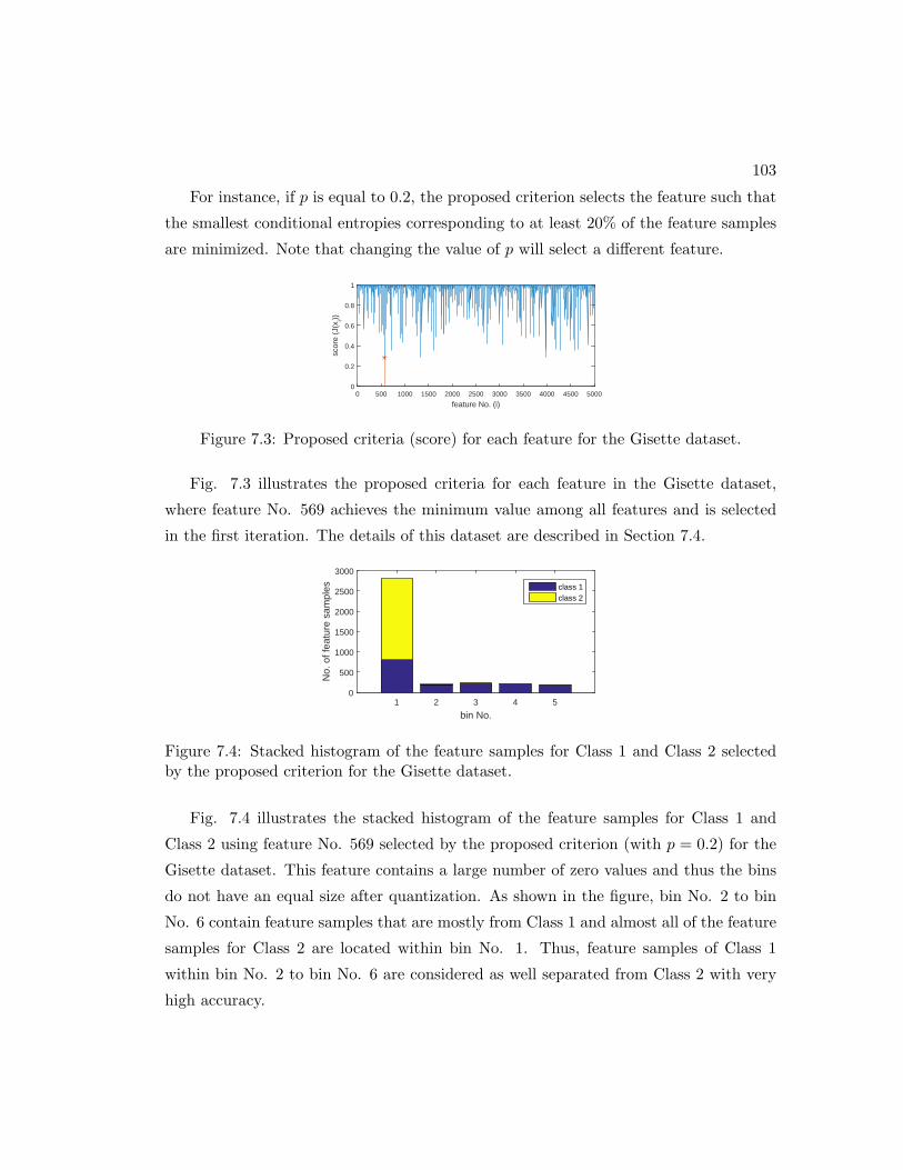
103
For instance, if p is equal to 0.2, the proposed criterion selects the feature such that
the smallest conditional entropies corresponding to at least 20% of the feature samples
are minimized. Note that changing the value of p will select a different feature.
feature No. (i)0 500 1000 1500 2000 2500 3000 3500 4000 4500 5000
scor
e (J
(xi))
0
0.2
0.4
0.6
0.8
1
Figure 7.3: Proposed criteria (score) for each feature for the Gisette dataset.
Fig. 7.3 illustrates the proposed criteria for each feature in the Gisette dataset,
where feature No. 569 achieves the minimum value among all features and is selected
in the first iteration. The details of this dataset are described in Section 7.4.
bin No.1 2 3 4 5
No.
of f
eatu
re s
ampl
es
0
500
1000
1500
2000
2500
3000
class 1class 2
Figure 7.4: Stacked histogram of the feature samples for Class 1 and Class 2 selectedby the proposed criterion for the Gisette dataset.
Fig. 7.4 illustrates the stacked histogram of the feature samples for Class 1 and
Class 2 using feature No. 569 selected by the proposed criterion (with p = 0.2) for the
Gisette dataset. This feature contains a large number of zero values and thus the bins
do not have an equal size after quantization. As shown in the figure, bin No. 2 to bin
No. 6 contain feature samples that are mostly from Class 1 and almost all of the feature
samples for Class 2 are located within bin No. 1. Thus, feature samples of Class 1
within bin No. 2 to bin No. 6 are considered as well separated from Class 2 with very
high accuracy.

104
Fig. 7.1 illustrates the histograms of (a) original feature No. 939 and (b) quantized
feature No. 939 selected by the proposed algorithm in the first iteration using Patient
No. 1 in the American Seizure Prediction Challenge database (see Section 7.4). As
opposed to the features in the Gisette dataset, this is a continuous feature and thus is
quantized into 20 different bins with equal size. As shown in the figure, bin No. 1-2
and bin No. 15-20 contain feature samples mostly from Class 2. Thus, feature samples
within these bins are considered as well separable from Class 1.
7.1.3 Elimination of feature samples
Similar to Adaboost which assigns more weights to the feature samples that are mis-
classified in the previous steps [93], after feature selection according to the proposed
criterion, feature samples within certain bins with a small conditional entropy of the
class label are discarded.
We first define the impurity of each bin as the minimum of the probability of Class
1 and the probability of Class 2 for each bin [80]. Suppose an impurity threshold is
predefined as T , then feature samples within the bins whose bin impurity is less than
T are discarded and are not considered in the next feature selection step. This step
guarantees that feature samples surviving after each iteration are harder to classify
using previously selected features and each iteration focuses on these feature samples
only. This is a key aspect of the proposed algorithm. Note that while p affects what
feature selected, T affects which samples are eliminated at a certain step.
bin No.0 1 2 3 4 5 6
bin
impu
rity
0
0.1
0.2
0.3
Figure 7.5: Bin impurities for the feature selected by the proposed criterion for theGisette dataset.

105
Fig. 7.5 illustrates the corresponding bin impurities of the feature shown in Fig. 7.4
for the Gisette dataset. The first bin has the highest bin impurity and the bin impurities
for bins No. 3-6 are all less than 0.1. If we predefine the impurity threshold T as 0.1,
then all feature samples within bin No. 3-6 are discarded and are not considered in the
next iteration.
bin No.0 5 10 15 20
bin
impu
rity
0
0.1
0.2
0.3
Figure 7.6: Bin impurities of the feature selected by the proposed criterion for PatientNo. 1 in the American Seizure Prediction Challenge database.
Fig. 7.6 illustrates the corresponding bin impurities for the feature shown in Fig. 7.1
for Patient No. 1 in the American Epilepsy Society (AES) Seizure Prediction Challenge
database . More than half of the bins have an impurity less than 0.1. If we predefine the
impurity threshold T as 0.1, then feature samples within these 16 bins whose impurities
are less than 0.1 are discarded and are not considered in the next iteration. Thus, ap-
proximately 80% of the feature samples will be discarded and remaining feature samples
are subjected to the next iteration of feature selection and elimination.
7.1.4 Repetition
Using the criterion proposed in Section 7.1.2 and the discarding rule in Section 7.1.3,
m features are selected by repeating the proposed two steps for m times.
Fig. 7.7. illustrates the stacked histogram of the feature samples for Class 1 and
Class 2 in the second feature selection iteration using the proposed algorithm (with
p = 0.2) for the Gisette dataset, where x axis represents the bin number and y axis
represents the number of feature samples. Bin No. 2-5 contain feature samples mostly
from Class 2 and almost all of the feature samples for Class 1 are located within bin
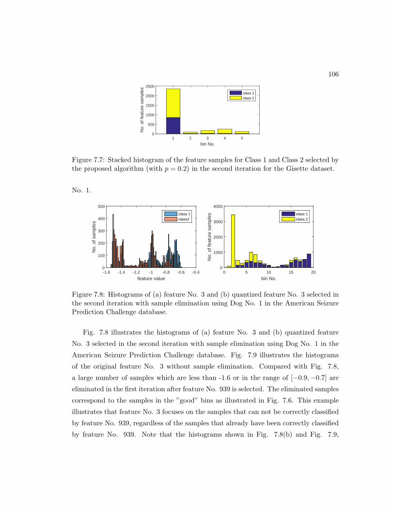
106
bin No.1 2 3 4 5
No.
of f
eatu
re s
ampl
es
0
500
1000
1500
2000
2500
class 1class 2
Figure 7.7: Stacked histogram of the feature samples for Class 1 and Class 2 selected bythe proposed algorithm (with p = 0.2) in the second iteration for the Gisette dataset.
No. 1.
feature value-1.6 -1.4 -1.2 -1 -0.8 -0.6 -0.4
No.
of s
ampl
es
0
100
200
300
400
500
class 1class2
bin No.0 5 10 15 20
No.
of f
eatu
re s
ampl
es
0
1000
2000
3000
4000
class 1class 2
Figure 7.8: Histograms of (a) feature No. 3 and (b) quantized feature No. 3 selected inthe second iteration with sample elimination using Dog No. 1 in the American SeizurePrediction Challenge database.
Fig. 7.8 illustrates the histograms of (a) feature No. 3 and (b) quantized feature
No. 3 selected in the second iteration with sample elimination using Dog No. 1 in the
American Seizure Prediction Challenge database. Fig. 7.9 illustrates the histograms
of the original feature No. 3 without sample elimination. Compared with Fig. 7.8,
a large number of samples which are less than -1.6 or in the range of [−0.9,−0.7] are
eliminated in the first iteration after feature No. 939 is selected. The eliminated samples
correspond to the samples in the ”good” bins as illustrated in Fig. 7.6. This example
illustrates that feature No. 3 focuses on the samples that can not be correctly classified
by feature No. 939, regardless of the samples that already have been correctly classified
by feature No. 939. Note that the histograms shown in Fig. 7.8(b) and Fig. 7.9,

107
feature value-2.5 -2 -1.5 -1 -0.5
No.
of s
ampl
es0
500
1000
1500
2000
2500class 1class2
Figure 7.9: Histograms of the original feature No. 3 without sample elimination.
respectively, correspond to 39375 and 7875 samples.
7.1.5 Summary
Algorithm 4 Algorithm for MUSE feature selection
Predefine p and TStart with the empty set S0 = {ϕ}, i = 0for i = 1 to m do
1. For each feature, compute and sort the conditional entropy such thatH(c|B1) <H(c|B2) < ... < H(c|BK)
2. For each feature, find the smallest K ′ such thatK′∑k=1
P (Bk) > p
3. Select the next best feature x∗ = argminx∈S
J(x) =K′∑k=1
P (Bk)H(c|Bk)
4. Si = Si−1 ∪ {x∗}5. Discard feature samples within the bins whose impurity is less than T
end for
In summary, the proposed feature selection algorithm is described in Algorithm 4.
Let pi represent the percentage of feature samples eliminated in the i-th iteration. The
parameter pi depends on T , and should not be confused with p. Denote bins whose
impurities are less than T as ”good”, and denote bins whose impurities are greater than
T as ”bad”. The proposed sample elimination process is illustrated in Fig. 7.10, where
at the i-th iteration, for samples that have not yet been eliminated, pi∏i−1
k=1(1 − pk)
feature samples are quantized into ”good” bins, and the remaining∏i
k=1(1−pk) feature
samples are quantized into ”bad” bins. Then at the i-th iteration of feature selection,
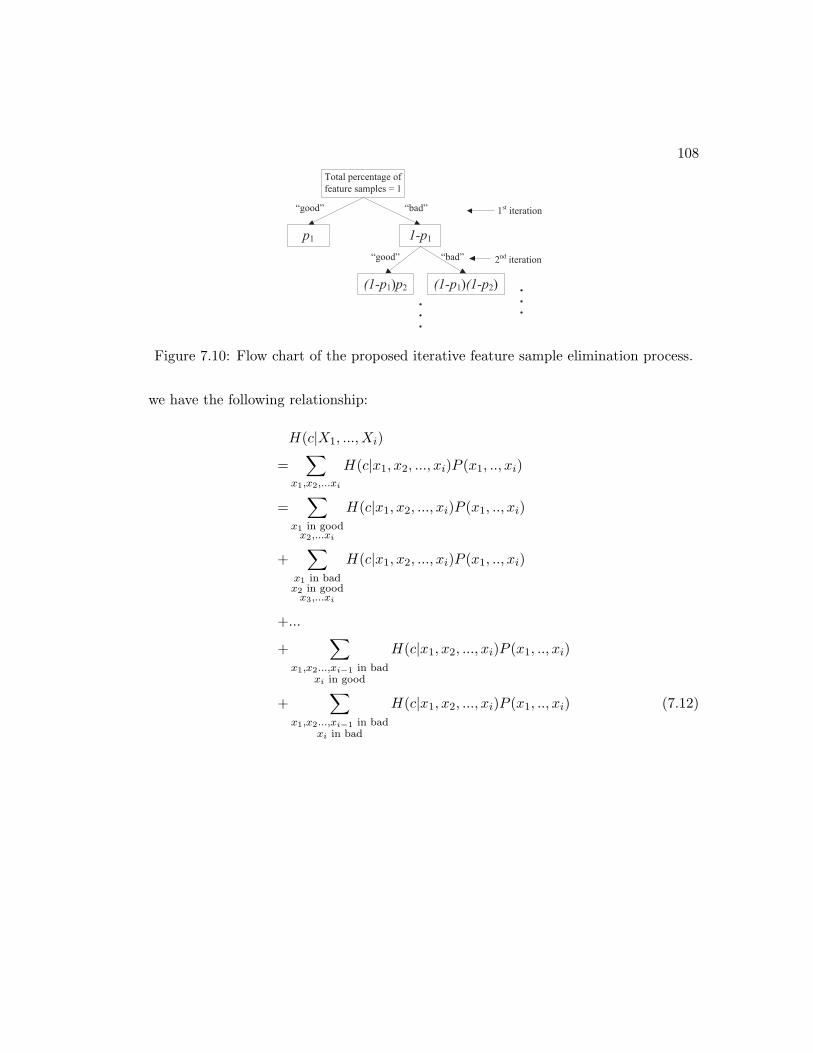
108
Total percentage of
feature samples = 1
p1 1-p1
1st iteration“good” “bad”
2nd iteration
(1-p1)p2
“good”
(1-p1)(1-p2)
“bad”
Figure 7.10: Flow chart of the proposed iterative feature sample elimination process.
we have the following relationship:
H(c|X1, ..., Xi)
=∑
x1,x2,...xi
H(c|x1, x2, ..., xi)P (x1, .., xi)
=∑
x1 in goodx2,...xi
H(c|x1, x2, ..., xi)P (x1, .., xi)
+∑
x1 in badx2 in goodx3,...xi
H(c|x1, x2, ..., xi)P (x1, .., xi)
+...
+∑
x1,x2...,xi−1 in badxi in good
H(c|x1, x2, ..., xi)P (x1, .., xi)
+∑
x1,x2...,xi−1 in badxi in bad
H(c|x1, x2, ..., xi)P (x1, .., xi) (7.12)
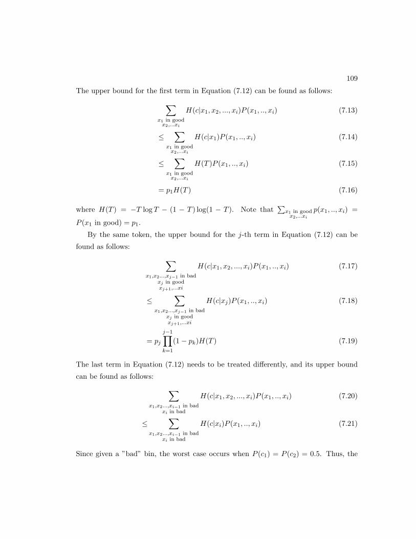
109
The upper bound for the first term in Equation (7.12) can be found as follows:∑x1 in goodx2,...xi
H(c|x1, x2, ..., xi)P (x1, .., xi) (7.13)
≤∑
x1 in goodx2,...xi
H(c|x1)P (x1, .., xi) (7.14)
≤∑
x1 in goodx2,...xi
H(T )P (x1, .., xi) (7.15)
= p1H(T ) (7.16)
where H(T ) = −T log T − (1 − T ) log(1 − T ). Note that∑
x1 in goodx2,...xi
p(x1, .., xi) =
P (x1 in good) = p1.
By the same token, the upper bound for the j-th term in Equation (7.12) can be
found as follows: ∑x1,x2...,xj−1 in bad
xj in goodxj+1,...xi
H(c|x1, x2, ..., xi)P (x1, .., xi) (7.17)
≤∑
x1,x2...,xj−1 in badxj in goodxj+1,...xi
H(c|xj)P (x1, .., xi) (7.18)
= pj
j−1∏k=1
(1− pk)H(T ) (7.19)
The last term in Equation (7.12) needs to be treated differently, and its upper bound
can be found as follows: ∑x1,x2...,xi−1 in bad
xi in bad
H(c|x1, x2, ..., xi)P (x1, .., xi) (7.20)
≤∑
x1,x2...,xi−1 in badxi in bad
H(c|xi)P (x1, .., xi) (7.21)
Since given a ”bad” bin, the worst case occurs when P (c1) = P (c2) = 0.5. Thus, the

110
upper bound of the last term in Equation (7.12) can be found as follows:∑x1,x2...,xi−1 in bad
xi in bad
H(c|x1, x2, ..., xi)P (x1, .., xi) (7.22)
≤∑
x1,x2...,xi−1 in badxi in bad
H(0.5)P (x1, .., xi) (7.23)
=
i∏k=1
(1− pk) (7.24)
In summary, the upper bound of H(c|X1, ..., Xi) can be written as follows:
H(c|X1, ..., Xi) (7.25)
≤i∑
j=1
pj
j−1∏k=1
(1− pk)H(T ) +i∏
k=1
(1− pk) (7.26)
=H(T ) + (1−H(T ))i∏
k=1
(1− pk) (7.27)
Since 1−H(T ) is always greater than 0 and I(c;X1, X2, ..., Xi) = H(c)−H(c|X1, ..., Xi),
the proposed algorithm iteratively increases the mutual information between selected
features and the class label as the upper bound of H(c|X1, ..., Xi) converges to H(T )
linearly with a rate equal to (1− pmin), where pmin = min{p1, p2, ..., pi}.
Table 7.1: Conditional Entropy for mRMR and the Proposed Method and its EstimatedValue.
# of features (i) 1 2 3 4
H(c|X1, ..., Xi) (mRMR) 0.2335 0.1159 0.0182 0.0016
H(c|X1, ..., Xi) (Proposed) 0.2335 0.1125 0.0064 0.0014
Estimated H(c|X1, ..., Xi) 0.2335 0.1401 0.0813 0.03941
Table 7.1 illustrates (a) the conditional entropy, referred as H(c|X1, ..., Xi), for m-
RMR, (b) the conditional entropy for the proposed method, and (c) the estimated
conditional entropy for the proposed method using Equation (27) after each iteration
of feature selection for Patient No. 1 in the American Seizure Prediction Challenge
dataset. The conditional entropy converges much faster to 0 than its estimated value
and the proposed method achieves a lower value than the mRMR. Note that the esti-
mated conditional entropy in the last row of Table 7.1 is an upper bound of the actual
conditional entropy in the row above the last row.

111
Fig. 7.11 illustrates the scatter plot of interictal features (represented by blue cross-
es) and preictal features (represented by red dots) using three features selected by the
proposed algorithm. As shown in the figure, the feature samples in the feature space
selected by the proposed algorithm are typically non-linearly separable for the following
reasons:
(1) The proposed criterion or score used for feature ranking in each iteration is a
non-linear metric that measures the non-linear relationship between the feature and
class label.
(2) Feature samples are also discarded in a non-linear way. As shown in Fig. 7.6,
after feature selection, feature samples within the lowest 2 bins and the highest 6 bins
are discarded.
1.51
feature NO. 14
0.50
-0.5-10
-1
feature NO. 471
-2
-0.4
-0.2
0
0.2
0.4
0.6
0.8
-3
feat
ure
NO
. 404
preictalinterictal
Figure 7.11: Scatter plot of interictal features (blue crosses) and preictal features (redcircles) using the features selected by the proposed algorithm for Patient No. 1 in theAmerican Seizure Prediction Challenge dataset.
7.2 Classifiers
To test the performance of the proposed algorithm, we consider four widely used classi-
fiers which include Naive Bayes (NB), Linear Discrimant Analysis (LDA), classification
and regression tree (CART), and artificial neural network (ANN).

112
7.3 Practical Issues
7.3.1 Quantization level
Since features need to be quantized into finite discrete values in the first step, the level
of quantization, i.e., the number of bins, needs to be determined first. In the mRMR
algorithm, different datasets use different discretization levels.
The data set HDR (Multiple Features Data Set) [133, 134, 135, 136] contains 649
features of 2,000 handwritten digits (from 0 to 9). To discretize the data set, each
feature variable was binarized at the mean value, i.e., it takes 1 if it is larger than the
mean value and -1 otherwise.
However, for the arrhythmia dataset, each feature variable was discretized into three
states at the positions µ±σ (µ represents the mean value and σ represents the standard
deviation): it takes -1 if it is less than µ−σ, 1 if larger than µ+σ, and 0 if otherwise.
We propose that the discretization level can be determined by estimating the error
rate first for different levels and then selecting a quantization level that achieves the
lowest error rate as the final level. Fig. 7.12 illustrates the classification error rate of
the Arrhythmia dataset for different quantization levels using (a) Naive Bayes classifier,
(b) LDA classifier, and (c) CART classifier. As shown in the figure, when Naive Bayes
classifier and LDA classifier are used, the proposed algorithm achieves the minimum
classification error rate when data is quantized into 9 bins. If CART is used as the
classifier, then the proposed algorithm achieves the 3rd minimum classification error rate
when data is quantized into 9 bins. Therefore, for this dataset, features are discretized
into 9 levels.
To guarantee a fair comparison, the quantization level for mRMR is the same as the
proposed algorithm.
7.3.2 Number of features
Even though an algorithm for selecting m features are proposed, in practice, the number
of features to select is usually unknown at the beginning until a classifier is trained. In
mRMR, to select the candidate feature set, the cross-validation classification error is first
computed for a large number of features and then the number of features is determined
so as to achieve a relatively stable range of small error. This requires the algorithm
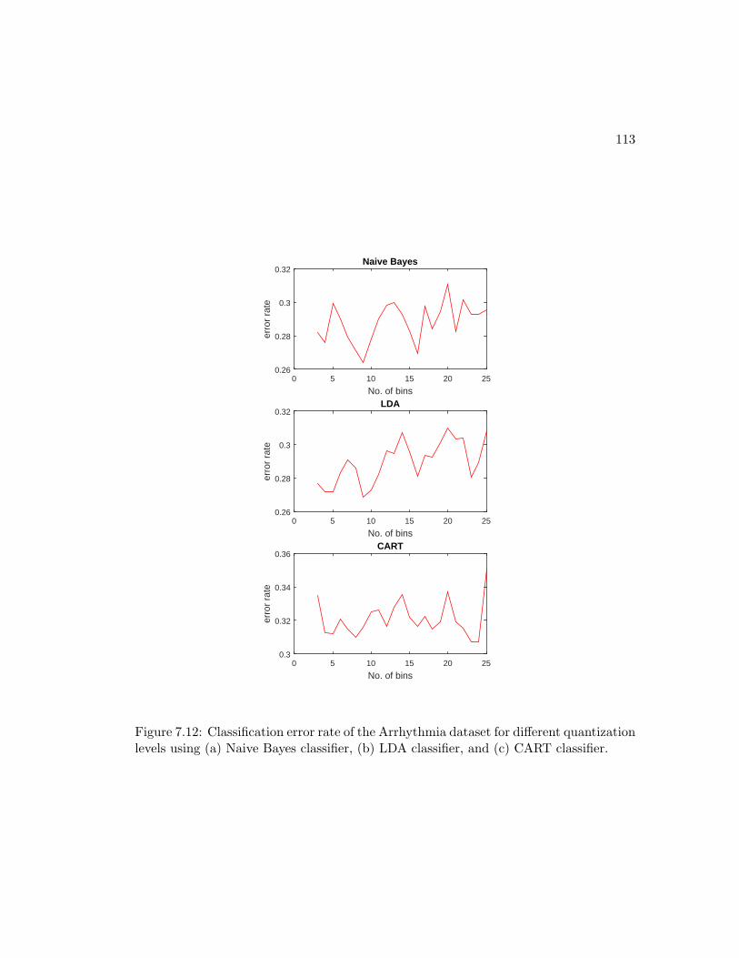
113
No. of bins0 5 10 15 20 25
erro
r ra
te
0.26
0.28
0.3
0.32Naive Bayes
No. of bins0 5 10 15 20 25
erro
r ra
te
0.26
0.28
0.3
0.32LDA
No. of bins0 5 10 15 20 25
erro
r ra
te
0.3
0.32
0.34
0.36CART
Figure 7.12: Classification error rate of the Arrhythmia dataset for different quantizationlevels using (a) Naive Bayes classifier, (b) LDA classifier, and (c) CART classifier.
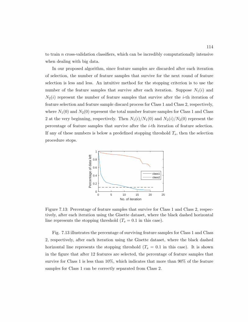
114
to train n cross-validation classifiers, which can be incredibly computationally intensive
when dealing with big data.
In our proposed algorithm, since feature samples are discarded after each iteration
of selection, the number of feature samples that survive for the next round of feature
selection is less and less. An intuitive method for the stopping criterion is to use the
number of the feature samples that survive after each iteration. Suppose N1(i) and
N2(i) represent the number of feature samples that survive after the i-th iteration of
feature selection and feature sample discard process for Class 1 and Class 2, respectively,
where N1(0) and N2(0) represent the total number feature samples for Class 1 and Class
2 at the very beginning, respectively. Then N1(i)/N1(0) and N2(i)/N2(0) represent the
percentage of feature samples that survive after the i-th iteration of feature selection.
If any of these numbers is below a predefined stopping threshold Ts, then the selection
procedure stops.
No. of iteration0 5 10 15 20 25
Per
cent
age
of d
ata
left
0
0.2
0.4
0.6
0.8
1
class1class2
Figure 7.13: Percentage of feature samples that survive for Class 1 and Class 2, respec-tively, after each iteration using the Gisette dataset, where the black dashed horizontalline represents the stopping threshold (Ts = 0.1 in this case).
Fig. 7.13 illustrates the percentage of surviving feature samples for Class 1 and Class
2, respectively, after each iteration using the Gisette dataset, where the black dashed
horizontal line represents the stopping threshold (Ts = 0.1 in this case). It is shown
in the figure that after 12 features are selected, the percentage of feature samples that
survive for Class 1 is less than 10%, which indicates that more than 90% of the feature
samples for Class 1 can be correctly separated from Class 2.

115
number of features0 1 2 3 4 5 6
perc
enta
ge o
f fea
ture
sam
ple
surv
ied
0
0.2
0.4
0.6
0.8
1
class 1 (interictal)class 2 (preictal)
Figure 7.14: Percentage of feature samples that survive for Class 1 (interictal) and Class2 (preictal), respectively, after each iteration for Patient No. 1 in the American SeizurePrediction Challenge database.
Fig. 7.14 illustrates the percentage of surviving feature samples for Class 1 (in-
terictal) and Class 2 (preictal), respectively, after each iteration for Patient No. 1 in
the AES Seizure Prediction Challenge database, where the black dashed horizontal line
represents the stopping threshold (Ts = 0.01 in this case). It is shown in the figure that
after 4 features are selected, the percentage of feature samples that survive for Class 1
is less than 1%, which indicates that more than 99% of the interictal feature samples of
Class 1 can be correctly separated from preictal features of Class 2. The threshold is
selected as small as 0.01 because of the large size of the interictal data.
7.4 Datasets
Three datasets are used in this chapter. These include the Arrhythmia and Gisette
datasets from UCI and the seizure prediction contest dataset containing data from 5
dogs and 2 humans from Kaggle. All data are publicly available. These datasets are
described below.
7.4.1 Arrhythmia dataset
The first dataset is the Arrhythmia dataset from UCI [137, 138, 139]. According to
[137], this database contains 279 attributes, 206 of which are linear valued and the rest
are nominal. The aim is to distinguish between the presence and absence of cardiac
arrhythmia and to classify it in one of the 16 groups. Class 01 refers to ’normal’ ECG

116
classes 02 to 15 refer to different classes of arrhythmia and Class 16 refers to the rest of
unclassified ones. The class label has two states with 237 and 183 samples, respectively.
7.4.2 Gisette dataset
The second dataset is the Gisette digit recognition dataset from UCI [140, 141, 142].
According to [140], the digits have been size-normalized and centered in a fixed-size
image of dimension 28x28. The original data were modified for the purpose of the
feature selection challenge. In particular, pixels were sampled at random in the middle
top part of the feature containing the information necessary to disambiguate 4 from 9
and higher order features were created as products of these pixels to plunge the problem
in a higher dimensional feature space. A number of distractor features called ’probes’
having no predictive power were also added to this dataset. The order of the features
and patterns were randomized.
Table 7.2 summarizes feature types, feature numbers, and number of feature samples
for the Arrhythmia dataset and the Gisette dataset.
Table 7.2: Description of Arrhythmia and Gisette datasets.
Dataset Arrhythmia Gisette
Source UCI UCI
Raw feature type Continuous integer
Quatization level 9 6
# of features 278 5000
# of samples 420 6000
Class # Name # of sample Name # of sample
Class 1 Normal 237 ”4” 3000
Class 2 Abnormal 183 ”9” 3000
Testing method 5-fold cross validation with permutations
7.4.3 American Epilepsy Society Seizure Prediction Challenge database
The third dataset is the American Epilepsy Society (AES) Seizure Prediction Challenge
database [129, 143]. Details of this dataset are described in Section 6.1. Table 7.3
summarizes the number of features, number of feature samples and number of dataclips
of the training set and testing set for each subject.

117
Two types of features are extracted from the EEG signals. These features include
relative spectral power and spectral power ratio. We use the same feature extraction
process as explained in detail in [27]. For the 5 canine subjects, 10 relative spectral
powers are extracted and(102
)= 45 spectral power ratios are computed from these
spectral powers from each electrode. For the 2 canine subjects, 13 relative spectral
powers are extracted and(132
)= 78 spectral power ratios are computed from these
spectral powers from each electrode.
Table 7.3: Seizure Prediction Dataset from Kaggle Contest.
DatasetAmerican Epilepsy Society Seizure Prediction Challenge
Dog 1 Dog 2 Dog 3 Dog 4 Dog 5 Pat. 1 Pat. 2
Source [129]
Raw feature type Continuous
Quatization level 20
# of electrodes 16 16 16 16 16 15 24
# of features/electrode 55 55 55 55 55 91 91
Total # of features 880 880 880 880 880 1365 2184
# of feature samples/clip 598 598 598 598 598 599 599
Training Set (# of clips)
Total 504 542 1512 901 480 68 60
Class 1 (Interictal) 480 500 1440 804 450 50 42
Class 2 (Preictal) 24 42 72 97 30 18 18
Testing Set (# of clips)
Total 502 1000 907 990 191 195 150
Class 1 (Interictal) 478 910 865 933 179 183 14
Class 2 (Preictal) 24 90 42 57 12 12 136
7.5 Experimental Results
7.5.1 Arrhythmia dataset
The details for testing the proposed algorithm on this dataset are described as follows:
1) Two important criteria for performance evaluation are used for this dataset which
include sensitivity and specificity. The sensitivity of a clinical test refers to the ability
of the test to correctly identify those patients with the disease and is defined as follows:
Sensitivity=True Positives/Positives
The specificity of a clinical test refers to the ability of the test to correctly identify those
patients without the disease and is defined as follows:

118
Specificity=True Negatives/Negatives
2) Five-fold cross-validation with permutation is used to achieve the averaged value
of sensitivity and specificity versus different number of features. Feature samples are
permuted first and partitioned into five equal size folds. Of the 5 folds, a single fold is
retained as the validation data for testing the model, and the remaining 4 folds are used
for training. The cross-validation process is then repeated 5 times, with each of the 5
folds used exactly once as the validation data. The 5 results from the folds can then
be averaged (or otherwise combined) to produce a single estimation. Such a process is
repeated for 500 times to achieve an ensemble results of the sensitivity and specificity
by averaging the 500 estimations.
Fig. 7.15(a), (b), and (c) compare the sensitivity (left panel) and specificity (right
panel) of the proposed algorithm and the mRMR algorithm for the Arrhythmia dataset
from UCI using (a) Naive Bayes classifier, (b) LDA classifier, and (c) CART, respec-
tively. As shown in the figures, when 5 features are selected, the proposed algorithm
achieves a significantly higher sensitivity than mRMR. The proposed algorithm achieves
30% higher sensitivity when Naive Bayes classifier is used and achieves approximately
20% higher sensitivity when CART classifier is used. On the other hand, the proposed
algorithm only achieves 7% less specificity when Naive Bayes classifier is used and 5%
less specificity when CART classifier is used.
7.5.2 Gisette dataset
The details for testing the proposed algorithm on this dataset are described as follows:
1) The criterion for performance evaluation used for this dataset is the classification
accuracy for Class 1 and Class 2.
2) Five-fold cross-validation with permutation is used to achieve the averaged value
of sensitivity and specificity versus different number of features. Feature samples are
permuted randomly first and partitioned into five equal size folds. Of the 5 folds, a
single fold is retained as the validation data for testing the model, and the remaining 4
folds are used for training. The cross-validation process is then repeated 5 times, with
each of the 5 folds used exactly once as the validation data. The 5 results from the folds
can then be averaged (or otherwise combined) to produce a single estimation. Such a
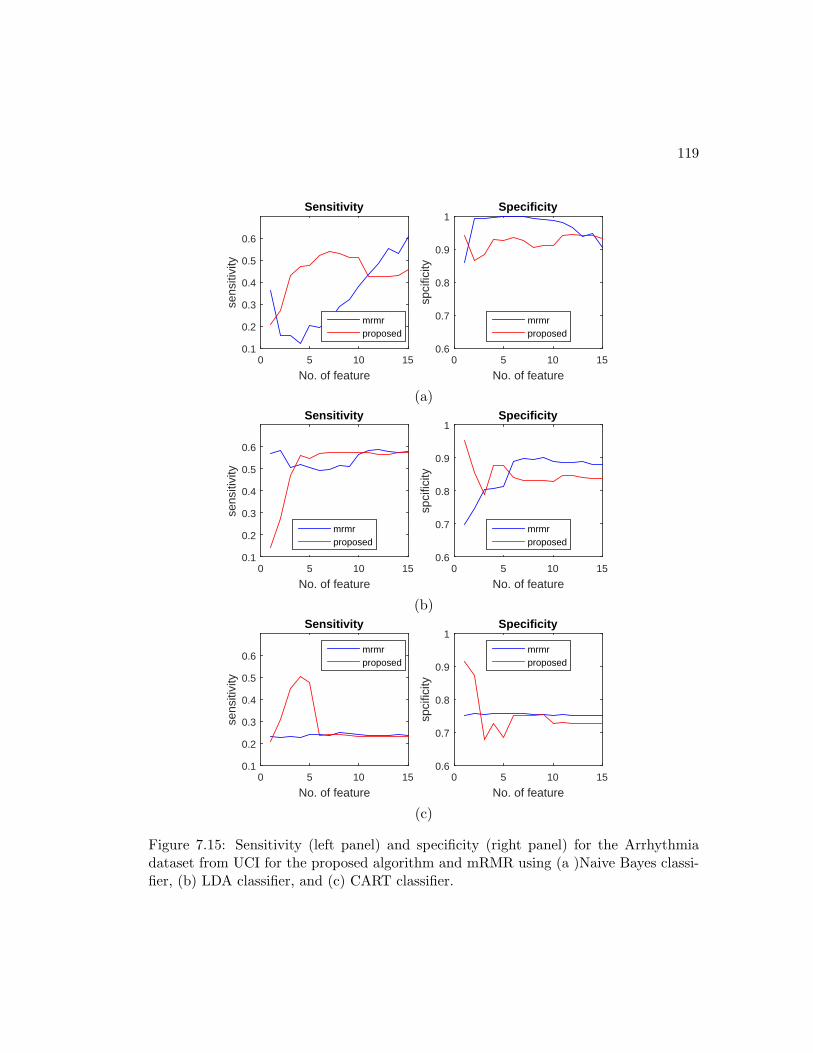
119
No. of feature0 5 10 15
sens
itivi
ty
0.1
0.2
0.3
0.4
0.5
0.6
Sensitivity
mrmrproposed
No. of feature0 5 10 15
spci
ficity
0.6
0.7
0.8
0.9
1Specificity
mrmrproposed
(a)
No. of feature0 5 10 15
sens
itivi
ty
0.1
0.2
0.3
0.4
0.5
0.6
Sensitivity
mrmrproposed
No. of feature0 5 10 15
spci
ficity
0.6
0.7
0.8
0.9
1Specificity
mrmrproposed
(b)
No. of feature0 5 10 15
sens
itivi
ty
0.1
0.2
0.3
0.4
0.5
0.6
Sensitivity
mrmrproposed
No. of feature0 5 10 15
spci
ficity
0.6
0.7
0.8
0.9
1Specificity
mrmrproposed
(c)
Figure 7.15: Sensitivity (left panel) and specificity (right panel) for the Arrhythmiadataset from UCI for the proposed algorithm and mRMR using (a )Naive Bayes classi-fier, (b) LDA classifier, and (c) CART classifier.

120
process is repeated for 500 times to achieve an ensemble results of the sensitivity and
specificity by averaging the 500 estimations.
Fig. 7.16 (a), (b), and (c) compare the classification accuracies of Class 1 (left panel)
and Class 2 (right panel) of the proposed algorithm and the mRMR for the Arrhythmia
dataset from UCI using (a) Naive Bayes classifier, (b) LDA classifier, and (c) CART,
respectively.
As shown in the figures, the proposed algorithm always starts with a high accuracy
for Class 1 and a low accuracy for Class 2. As the number of features increases, the
proposed algorithm achieves approximately the same accuracy as the mRMR for both
Class 1 and Class 2 when the LDA and CART classifiers are used. However, when Naive
Bayes classifier is used, the proposed algorithm has a 3% lower accuracy for Class 1 and
15% higher accuracy for Class 2.
7.5.3 American Epilepsy Society Seizure Prediction Challenge database
Table 7.4: Classification Performance on the American Epilepsy Society Seizure Predic-tion Challenge database Using CART
DatasetAmerican Epilepsy Society Seizure Prediction Challenge databaseDog 1 Dog 2 Dog 3 Dog 4 Dog 5 Pat. 1 Pat. 2
# of feature 10 10 10 10 10 4 4
AUC(proposed) 0.7708 0.8359 0.7095 0.8499 0.6311 0.8272 0.7629
AUC(mRMR) 0.7495 0.7528 0.6304 0.7670 0.4774 0.6430 0.6179
SS(proposed) 0.6667 0.7556 0.5952 0.7719 0.6667 0.7500 0.6429
SS(mRMR) 0.6715 0.6667 0.6190 0.7719 0.5000 0.5833 0.5714
SP(proposed) 0.6667 0.8077 0.7341 0.8006 0.6313 0.7760 0.7647
SP(mRMR) 0.7197 0.7549 0.6220 0.6613 0.5307 0.5847 0.7426
The details for the proposed algorithm are described as follows:
1) Three important criteria for performance evaluation are used for this dataset
which include sensitivity, specificity, and area under curve (AUC).
2) Training set is used for feature selection and classifier training. Ground truth
for testing is known beforehand and thus are used for validation, i.e., selecting the best
feature subset selected by the proposed algorithm and mRMR and then a corresponding
classifier.
3) Due to the imbalance between the data size of the preictal features and the
interictal features, random subsampling, which refers to randomly selecting a subset of
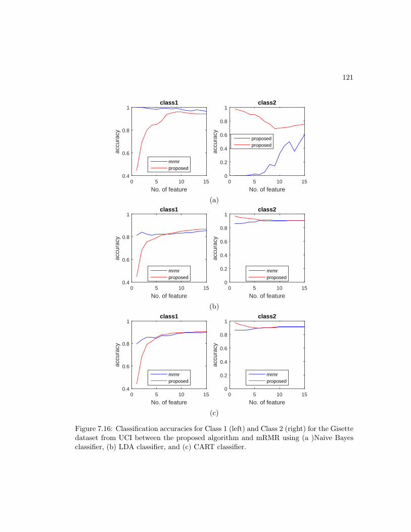
121
No. of feature0 5 10 15
accu
racy
0.4
0.6
0.8
1class1
mrmrproposed
No. of feature0 5 10 15
accu
racy
0
0.2
0.4
0.6
0.8
1class2
proposedproposed
(a)
No. of feature0 5 10 15
accu
racy
0.4
0.6
0.8
1class1
mrmrproposed
No. of feature0 5 10 15
accu
racy
0
0.2
0.4
0.6
0.8
1class2
mrmrproposed
(b)
No. of feature0 5 10 15
accu
racy
0.4
0.6
0.8
1class1
mrmrproposed
No. of feature0 5 10 15
accu
racy
0
0.2
0.4
0.6
0.8
1class2
mrmrproposed
(c)
Figure 7.16: Classification accuracies for Class 1 (left) and Class 2 (right) for the Gisettedataset from UCI between the proposed algorithm and mRMR using (a )Naive Bayesclassifier, (b) LDA classifier, and (c) CART classifier.

122
the feature observations, are performed on the interictal features during training phase.
On the other hand, upsampling, which refers to duplicating the feature observations, are
performed on the preictal features. The two techniques are used together to ensure that
the preictal features contain approximately the same amount of feature observations as
the initerictal features.
4) Different feature sample subsets after random subsampling may lead to different
feature sets selected by mRMR or the proposed algorithm. Therefore, such random
sampling and feature selection steps are repeated for 100 times and the feature set that
achieves the highest AUC after training is selected as the final feature set.
5) Feature samples in each dataclip is classified as 0 (interictal) or 1 (preictal) after
classification. The probability for each data clip to be a preictal clip is computed as
averaging the class labels for all feature observations from the clip:
P (data clip=preictal) = Mean[class label of feature observations in the data clip]
6) CART and ANN are trained as the classifier for the this dataset and the perfor-
mance are evaluated.
Table 7.4 shows the highest AUC of the 100 experiments and its corresponding
sensitivity (SS) and specificity (SP) on the testing dataset for each subject when CART
is used. Fig. 7.17(a), (b), and (c) plot the AUC, sensitivity and specificity for each
subject, respectively. The proposed algorithm achieves a higher AUC for all subjects in
this dataset. The proposed algorithm achieves higher sensitivities for 5 out of 7 subjects
and achieves higher specificities for 6 out of 7 subjects in the dataset. In addition, the
proposed algorithm has a better overall classification accuracy than mRMR. When
CART is used, the proposed method achieves a higher AUC of 10.70% on average, a
higher sensitivity of 6.65% on average, and a higher specificity of 8.07% on average. A
two-sample t-test for the null hypothesis that the proposed algorithm achieves the same
AUC as mRMR is performed at the 5% significance level, where alternative hypothesis
is to evaluate whether mean AUC for the proposed algorithm is significantly higher than
mRMR. The test results achieve a p-value of 0.0258 that is low enough to reject the
null alternative and accept the alternative hypothesis.
Table 7.5 shows the highest AUC of the 100 experiments and its corresponding
sensitivity (SS) and specificity (SP) on the testing dataset for each subject when ANN
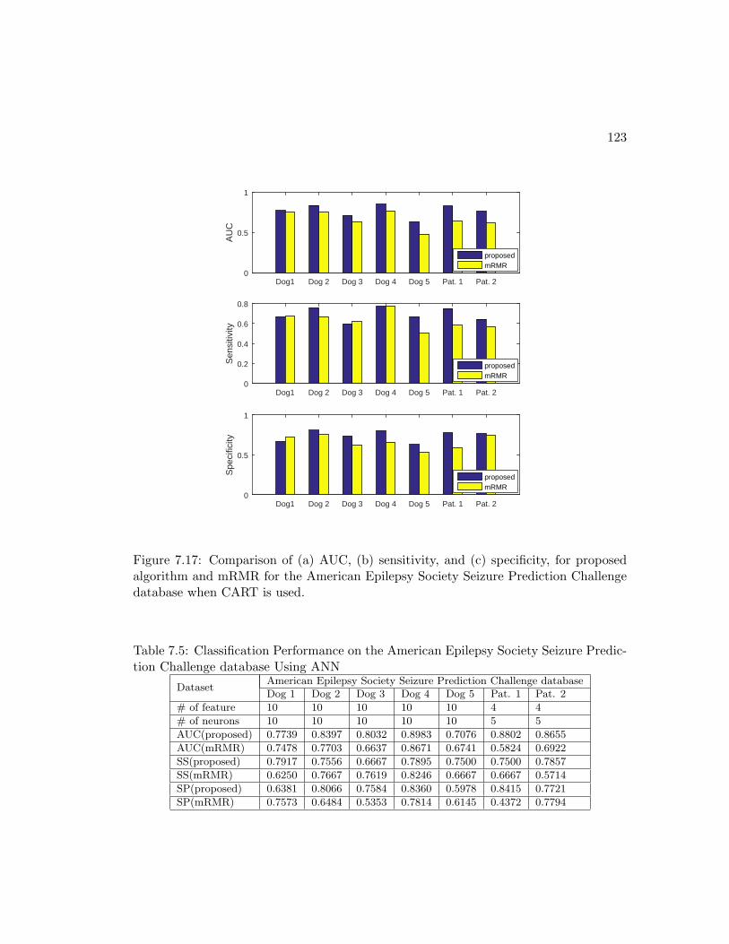
123
Dog1 Dog 2 Dog 3 Dog 4 Dog 5 Pat. 1 Pat. 2
AU
C
0
0.5
1
proposedmRMR
Dog1 Dog 2 Dog 3 Dog 4 Dog 5 Pat. 1 Pat. 2
Sen
sitiv
ity
0
0.2
0.4
0.6
0.8
proposedmRMR
Dog1 Dog 2 Dog 3 Dog 4 Dog 5 Pat. 1 Pat. 2
Spe
cific
ity
0
0.5
1
proposedmRMR
Figure 7.17: Comparison of (a) AUC, (b) sensitivity, and (c) specificity, for proposedalgorithm and mRMR for the American Epilepsy Society Seizure Prediction Challengedatabase when CART is used.
Table 7.5: Classification Performance on the American Epilepsy Society Seizure Predic-tion Challenge database Using ANN
DatasetAmerican Epilepsy Society Seizure Prediction Challenge databaseDog 1 Dog 2 Dog 3 Dog 4 Dog 5 Pat. 1 Pat. 2
# of feature 10 10 10 10 10 4 4
# of neurons 10 10 10 10 10 5 5
AUC(proposed) 0.7739 0.8397 0.8032 0.8983 0.7076 0.8802 0.8655
AUC(mRMR) 0.7478 0.7703 0.6637 0.8671 0.6741 0.5824 0.6922
SS(proposed) 0.7917 0.7556 0.6667 0.7895 0.7500 0.7500 0.7857
SS(mRMR) 0.6250 0.7667 0.7619 0.8246 0.6667 0.6667 0.5714
SP(proposed) 0.6381 0.8066 0.7584 0.8360 0.5978 0.8415 0.7721
SP(mRMR) 0.7573 0.6484 0.5353 0.7814 0.6145 0.4372 0.7794

124
is used. Fig. 7.18(a), (b), and (c) plot the AUC, sensitivity and specificity listed in Table
7.2 for each subject, respectively. As shown in the table and the figures, the proposed
algorithm achieves a higher AUC for all subjects in this dataset. The proposed algorithm
achieves higher sensitivities for 4 out of 7 subjects and achieves higher specificities for
4 out of 7 subjects in the dataset. In addition, the proposed algorithm has a better
overall classification accuracy than mRMR. When ANN is used, the proposed method
achieves a higher AUC of 11.01% on average, a higher sensitivity of 5.80% on average,
and a higher specificity of 9.96% on average. A two-sample t-test for the null hypothesis
that the proposed algorithm achieves the same AUC as mRMR is performed at the 5%
significance level, where alternative hypothesis is to evaluate whether mean AUC for
the proposed algorithm is significantly higher than mRMR. The test results achieve
a p-value of 0.0129 that is low enough to reject the null alternative and accept the
alternative hypothesis.
7.6 Discussion
In our approach, we stressed the importance for selecting a feature that focuses on the
samples that previously selected features are unable to separate into different classes.
In each step, surviving feature samples are ranked according to an uncertainty score
based on conditional entropies. In the next step, feature samples are further discarded
according to the bin impurities. Feature samples within the bins that have strong
predictive power to separate different classes are discarded. Thus, the proposed method
is more and more efficient and requires significantly less storage space after each iteration
since more and more samples are eliminated.
Our experimental results show that the proposed algorithm has different perfor-
mances depending on the dataset size and the types of classifiers.
For small datasets such as the Arrhythmia and Gisette datasets that contain only
hundreds or thousands of feature samples, the proposed algorithm, in general, may not
achieve a better classification performance when small number of features are selected.
The key reason is that classification variances for small datasets are very high. When
more and more features are selected, the proposed algorithm achieves approximately
the same classification performance as mRMR. The explanation for this is that as more
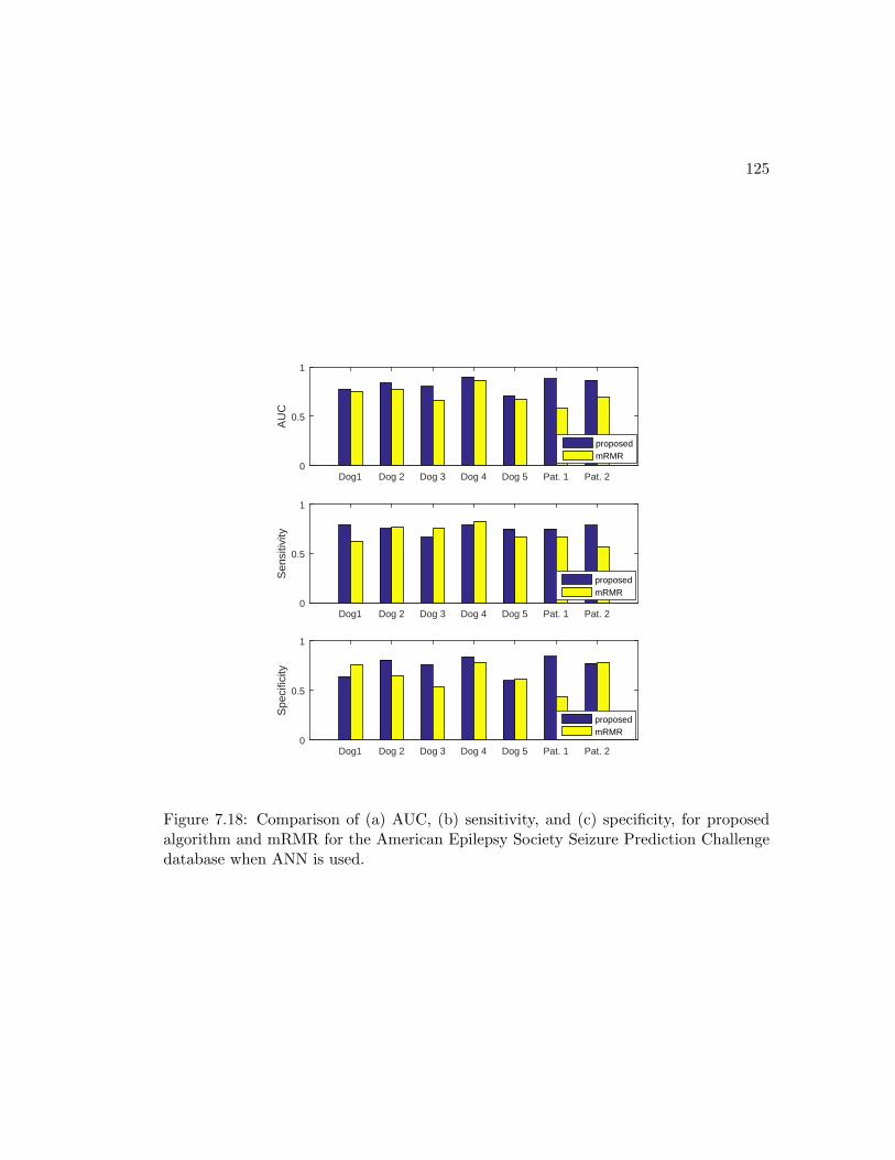
125
Dog1 Dog 2 Dog 3 Dog 4 Dog 5 Pat. 1 Pat. 2
AU
C
0
0.5
1
proposedmRMR
Dog1 Dog 2 Dog 3 Dog 4 Dog 5 Pat. 1 Pat. 2
Sen
sitiv
ity
0
0.5
1
proposedmRMR
Dog1 Dog 2 Dog 3 Dog 4 Dog 5 Pat. 1 Pat. 2
Spe
cific
ity
0
0.5
1
proposedmRMR
Figure 7.18: Comparison of (a) AUC, (b) sensitivity, and (c) specificity, for proposedalgorithm and mRMR for the American Epilepsy Society Seizure Prediction Challengedatabase when ANN is used.

126
and more feature samples are discarded, the new selected feature focuses only on a very
small portion of the original dataset. Thus, selected features may lead to overfitting if
the surviving data size is too small.
For big datasets such as the American Epilepsy Society Seizure Prediction Chal-
lenge database that contains hundreds of thousands of feature samples, the proposed
algorithm has a much better classification performance than mRMR in terms of AUC,
sensitivity and specificity when the same number of features are selected. Since hun-
dreds or even thousands of feature samples can survive further selection after a few
iterations of feature selection, over-fitting will not be a major concern for big data ap-
plications. Experimental results shows that for both CART and ANN classifiers, the
proposed algorithm achieves a significantly higher AUC on average. Statistical tests
illustrate that the proposed algorithm achieves a p-value low enough to conclude the
proposed algorithm has a better performance than mRMR.
In addition, the proposed algorithm achieves a better classification performance
when a non-linear classifier such as Naive Bayes classifier or CART is used.
7.7 Conclusion
A new recursive feature selection method has been presented in this chapter. Our
feature selection method places more emphasis on feature samples that are harder to
separate using selected features and thus avoids redundancy with selected features. We
show that the feature samples in the selected features space are non-linearly separable.
We also address the practical issues with regard to selecting data quantization level and
the number of features to select for given a dataset.
The performance analysis shows that for small datasets, the proposed algorithm
the proposed algorithm may not achieve better performance than mRMR when few
features are selected. As more and more features are selected, performance of the
proposed algorithm is approximately the same as mRMR. However, for big datasets
that contain hundreds of thousands or even millions of feature samples, our proposed
algorithm achieves a much better performance than mRMR in terms of AUC, sensitivity
and specificity. The proposed method is also more efficient and requires significantly
less storage space after each iteration than mRMR.

Chapter 8
M3U: Minimum Mean Minimum
Uncertainty Feature Selection For
Multiclass Classification
A new multi-class feature selection criterion is proposed based on minimum uncertain-
ty [99]. Fig. 8.1 illustrates a typical flow chart for machine learning, where f(n) =
[f1(n), ..., fL(n)]T represents the n-th feature vector (feature observation) with L fea-
tures extracted at time step n, and fi(n) is defined as the n-th feature sample of the
i-th feature. In this chapter, we propose a three-step algorithm that first quantizes
features into bins, computes an uncertainty vector for each feature and all sample in
each feature, and finally iteratively selects features that achieves the minimum mean
minimum uncertainty (M3U). The one-versus-all (OVA) uncertainty vector is defined
in Section 8.1.2. Given a feature sample in a particular feature, this uncertainty score
illustrates how good the bin (corresponding to the feature sample) is to separate the
class (corresponding to the feature sample) from the remaining classes. To the best of
our knowledge, this is a new sample-wise criterion that has not been proposed before.
The proposed iterative feature selection algorithm includes two minimization steps and
one expectation step, which include (1) find the minimum uncertainty (MU) score for
each feature sample given a feature subset, (2) compute the mean minimum uncertainty
score (M2U) for the feature subset, and (3) select the feature that achieves the minimum
127

128
mean minimum uncertainty score (M3U).
Input
signals
ClassificationFeature
Extraction
Decision
Figure 8.1: A typical flow chart for machine learning.
8.1 Proposed Method
In this chapter, a novel multiclass feature selection algorithm that outperforms mRMR
is proposed. The ultimate goal of the proposed algorithm is to select a feature subset
such that, for each feature vector, there exists a feature that has a low uncertainty
value in the selected feature subset. Fig. 8.2 illustrates the flow chart for the proposed
feature selection algorithm. The proposed algorithm includes two minimization steps
and one expectation step. Features are quantized into different bins at the first step.
The proposed feature selection method uses sample-wise uncertainty vector defined in
Section 8.1.2 (using weighted conditional entropy) as its criterion. A low uncertainty
score for a feature sample in a particular feature implies that this feature sample can
be well separated from feature samples from other classes. The proposed method then
computes the uncertainty vector for each feature. Starting with an empty feature subset,
the iterative feature selection method selects a feature in each iteration by (1) computing
the minimum uncertainty score for each feature sample for all possible feature subset
candidates, (2) computing the average minimum uncertainty score across all feature
samples, and (3) selecting the feature that achieves the minimum of the average value
of the minimum uncertainty score.
8.1.1 Feature quantization
Continuous feature
Quantization is the procedure of constraining the feature from a continuous set of val-
ues to a relatively small discrete set [42]. Suppose the amplitude of a signal x takes on
values over an interval from xmin to xmax, quantization of this signal into K levels can
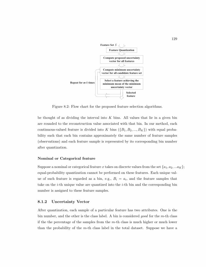
129
Feature Set
Feature Quantization
Selected
feature
Repeat for m-1 times
Compute proposed uncertainty
vector for all features
Select a feature achieving the
minimum mean of the minimum
uncertainty vector
Compute minimum uncertainty
vector for all candidate feature set
Figure 8.2: Flow chart for the proposed feature selection algorithms.
be thought of as dividing the interval into K bins. All values that lie in a given bin
are rounded to the reconstruction value associated with that bin. In our method, each
continuous-valued feature is divided into K bins ({B1, B2, ..., BK}) with equal proba-
bility such that each bin contains approximately the same number of feature samples
(observations) and each feature sample is represented by its corresponding bin number
after quantization.
Nominal or Categorical feature
Suppose a nominal or categorical feature x takes on discrete values from the set {a1, a2, ...aK};equal-probability quantization cannot be performed on these features. Each unique val-
ue of such feature is regarded as a bin, e.g., Bi = ai, and the feature samples that
take on the i-th unique value are quantized into the i-th bin and the corresponding bin
number is assigned to these feature samples.
8.1.2 Uncertainty Vector
After quantization, each sample of a particular feature has two attributes. One is the
bin number, and the other is the class label. A bin is considered good for the m-th class
if the the percentage of the samples from the m-th class is much higher or much lower
than the probability of the m-th class label in the total dataset. Suppose we have a
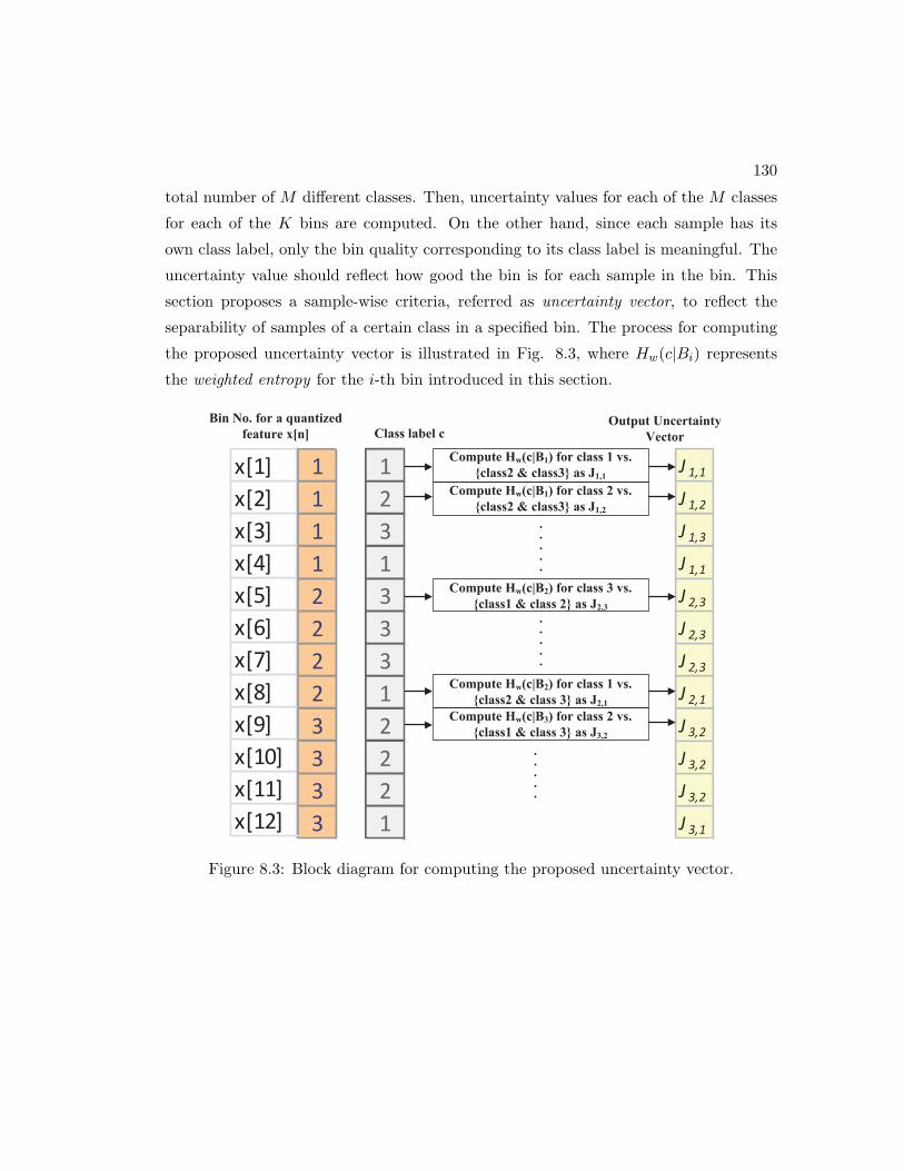
130
total number of M different classes. Then, uncertainty values for each of the M classes
for each of the K bins are computed. On the other hand, since each sample has its
own class label, only the bin quality corresponding to its class label is meaningful. The
uncertainty value should reflect how good the bin is for each sample in the bin. This
section proposes a sample-wise criteria, referred as uncertainty vector, to reflect the
separability of samples of a certain class in a specified bin. The process for computing
the proposed uncertainty vector is illustrated in Fig. 8.3, where Hw(c|Bi) represents
the weighted entropy for the i-th bin introduced in this section.
1
1
1
1
2
2
2
2
3
3
3
3
Bin No. for a quantized
feature x[n]
x[1]
x[2]
x[3]
x[4]
x[5]
x[6]
x[7]
x[8]
x[9]
x[10]
x[11]
x[12]
Compute Hw(c|B1) for class 1 vs.
{class2 & class3} as J1,11
2
3
1
3
3
3
1
2
2
2
1
Class label c
Compute Hw(c|B1) for class 2 vs.
{class2 & class3} as J1,2
Compute Hw(c|B2) for class 3 vs.
{class1 & class 2} as J2,3
Compute Hw(c|B2) for class 1 vs.
{class2 & class 3} as J2,1Compute Hw(c|B3) for class 2 vs.
{class1 & class 3} as J3,2
J 1,1
J 1,2
J 1,3
J 1,1
J 2,3
J 2,3
J 2,3
J 2,1
J 3,2
J 3,2
J 3,2
J 3,1
Output Uncertainty
Vector
Figure 8.3: Block diagram for computing the proposed uncertainty vector.

131
Let Bj represent the j-th bin after quantization in the first step. The mutual infor-
mation between the class label and the feature x can be written as:
I(x; c) = H(c)−H(c|x) (8.1)
= H(c)−∑j
H(c|x ∈ Bj)P (x ∈ Bj) (8.2)
where H(c) represents the entropy of the class label and is defined as follows:
H(c) =∑j
−P (cj) logP (cj), (8.3)
cj represents the j-th class label, and H(c|Bi) represents the conditional entropy of class
label given Bi and is defined as follows:
H(c|Bi) =∑j
−P (cj |x ∈ Bi) logP (cj |x ∈ Bi) (8.4)
Since given the class label, H(c) is a fixed number for all features, finding a feature
that maximizes equation (10) is equivalent to finding a feature such that the following
criterion is minimized:
maxxj∈X
[I(xj ; c)] (8.5)
⇔ minxj∈X
∑i
P (Bi)H(c|Bi) (8.6)
Therefore, a feature selected in the first step of mRMR is the feature such that the
expectation of the conditional entropies of the class labels for all bins is minimized.
However, this criterion suffers from inherent limitation of an imbalanced dataset. As
shown in Fig. 8.3, the entropy is computed for each feature sample for its corresponding
class (positive class) versus the remaining classes (negative class). In multiclass classifi-
cation problem, the two opposite classes are always very imbalanced. Suppose that the
dataset contains N1 and N2 feature samples from the positive class and the negative
class, respectively. Then H(c|Bi) can be computed as follows:
H(c|Bi) = −P (c+|x ∈ Bi) logP (c+|x ∈ Bi) (8.7)
− P (c−|x ∈ Bi) logP (c−|x ∈ Bi) (8.8)

132
0 0.5 10
0.5
1
Pr(X = 1)
y_
Figure 8.4: Binary entropy.
The relationship between conventional binary entropy and the probability for one class
is shown in Fig. 8.4, where the entropy value achieves the maximum when Pr(X =
1) = 0.5.
Suppose that data are very imbalanced such that N1 << N2, then H(c|Bi) has a
small value for all i, causing all bins to have a low entropy value. Therefore, we propose a
weighted entropy as the criterion in evaluating the predictive power of a bin. In general,
this criterion considers the imbalance between feature samples from two different classes
and is mathematically computed as follows:
Hw(c) = − wP+
wP+ + P−log(
wP+
wP+ + P−) (8.9)
− P−wP+ + P−
log(P−
wP+ + P−) (8.10)
where P+, P− represent the probabilities for the positive class and the negative class,
respectively, and w represents the weight factor and can be set as w = N2/N1. Figure
8.5 illustrates the relationship between the modified entropy and the probability for
class 1 with w = N2/N1 = 4, where the entropy value achieves the maximum at P (c =
1) = 0.2 = 11+w . Thus, a bin is considered bad for the positive class if the percentage
of the positive class is approximately equal to the probability of that class (expected
occurrence rate) in the entire dataset, and is considered good if the percentage of the
positive class is much higher or lower than its expected occurrence rate. For a given
feature x[n], n = 1, ..., N , containing N samples, we propose an algorithm as shown in
Fig. 8.3 to compute a one-versus-all (OVA) uncertainty vector u[n], n = 1, ..., N for
multi-class feature selection. The OVA uncertainty vector has the same size as the
given feature and each element in the vector represents the uncertainty value for each
sample against all the remaining samples from other classes. The detailed algorithm is

133
Pr(c=1)0 0.2 0.4 0.6 0.8 1
Hw(C
)
0
0.2
0.4
0.6
0.8
1
Figure 8.5: Binary entropy.
Algorithm 5 Algorithm for Computing the Uncertainty Vector for a Given Feature
Given a quantized feature x[n], n = 1, ..., N (with quantization level K) and the classlabel c with M different classesfor i = 1 to M do
Take feature samples from ci as one class (C+) and all the remaining featuresamples from other classes as the opposite class (C−)
for j = 1 to K doCompute Ji,j = Hw(C|Bi)
end forend forfor n = 1 to N do
Find uncertainty value u[n] for the n-th feature sample x[n] using its correspondingclass label and bin number.end for
illustrated in Algorithm 5.
Table 8.1 shows an example for a quantized feature with 5 bins and 4 classes. Each
class has 100 data points and each bin contains 80 samples since equal-size quantization
is used. Thus, the expected occurrence or observations in each bin for any class is 20.
As shown in the table, 50% of the samples of this feature in bin No. 1 are from class
1, which is significantly higher than its probability, i.e., 25%. Therefore, for samples of
class 1, bin No. 1 should be considered a good bin. However, for class 2 and class 3 in
this bin, their proportions are approximately the same as their expected probabilities.
Thus, bin No. 1 should be considered bad for class 2 and class 3. Similarly, bin No. 2,
bin No. 3, and bin No. 4 should be considered good for class 2, class 3, and class 4,
respectively. In summary, for this feature, the majority samples in the i-th bin come
from the i-th class.

134
Table 8.1: An Example For A Quantized Feature With 5 Bins And 4 Classes.No. of samples Bin 1 Bin 2 Bin 3 Bin 4 Bin 5 Total
Class1 40 10 10 10 30 100
Class2 15 45 10 10 20 100
Class3 15 10 45 10 20 100
Class4 10 15 15 50 10 100
Total 80 80 80 80 80 400
Table 8.2: Entropy With Weighting For The Features Shown in Table 8.1.
ji
Bin 1 Bin 2 Bin 3 Bin 4 Bin 5
Class 1 0.8113 0.8813 0.8813 0.8813 0.9402
Class 2 0.9760 0.7335 0.8813 0.8813 1
Class 3 0.9760 0.8813 0.7335 0.8813 1
Class 4 0.8813 0.9760 0.9760 0.6500 0.8813
The proposed entropy with weighting for the i-th bin and the j-th class, referred as
Ji,j , for this feature is shown in Table 8.2. For instance, for samples from Class 1 in bin
No. 1, J1,1 is evaluated for Class 1 against the remaining classes (i.e., { Class 2, Class
3, Class 4}) using w = 300/100 = 3 as the size of { Class 2, Class 3, Class 4} in the
total dataset is 3 times the size of Class 1 in the total dataset. As shown in the table,
Ji,j achieves a low score (shown in green) for the green samples in Table 8.1. On the
other hand, Ji,j achieves a high score (shown in red) for the red samples in Table 8.1.
The entropy without weighting for the i-th bin and the j-th class for this feature is
shown in Table 8.3. However, as shown in the table, Ji,j has a high uncertainty score
for the green samples in Table 8.1. Such values are counter intuitive as a high value
indicates that the i-th bin has low predictive power for the i-th class. In contrast, the
corresponding values obtained using weighted entropy in Table 8.2 are low; therefore,
these are more predicable as expected. This simple example illustrates the motivation
for the new uncertainty based method.
Table 8.3: Entropy Without Weighting For The Features Shown in Table 8.1.
ji
Bin 1 Bin 2 Bin 3 Bin 4 Bin 5
Class 1 1 0.5436 0.5436 0.5436 0.9544
Class 2 0.6962 0.9887 0.5436 0.5436 0.8113
Class 3 0.6962 0.5436 0.9887 0.5436 0.8113
Class 4 0.5436 0.6962 0.6962 0.9544 0.5436

135
8.1.3 Iterative Feature Selection
This section describes the proposed iterative feature selection method. Assume that
the total number of features is L. The selection goal is to select a subset of features
such that more and more feature vectors have a low uncertainty value. Let um[n],m =
1, ..., L, n = 1, ..., N represent the uncertainty vector for the m-th feature and the n-
th feature sample. This vector is computed using Algorithm 1 for each feature. Let Si
represent the feature subset selected in the i-th iteration. The iterative feature selection
algorithm can be described as follows:
(a) In the i-th iteration, each of the candidate features that has not yet been selected
is grouped with the selected feature subset to form a temporary feature subset Si,l
as Si = {Si−1, l}.
(b) Compute minimum uncertainty (MU) for each feature sample as the minimum
uncertainty score of the selected features.
(c) Compute the mean minimum uncertainty (M2U) for the feature Si,l by averaging
the minimum uncertainty (MU) score of all feature samples.
(d) Select the feature that achieves the minimum mean minimum uncertainty (M3U).
The detailed description of proposed selection method is illustrated in Algorithm 6.
An example for the proposed iterative feature selection algorithm is illustrated in
Fig. 8.6 using the weighted conditional entropies, where feature No. 1 is selected in
the first iteration as it achieves the minimum mean uncertainty score. In the second
iteration, feature No. 2 is grouped with feature No. 1 and the minimum is taken
between the two uncertainty vectors to compute a minimum uncertainty vector for the
2 features. Same process is repeated for feature No. 1 and feature No. 3. Since the
mean of the minimum uncertainty vector for feature No. 1 and feature No. 2 is lower
than that of feature No. 1 and feature No. 3, feature No. 2 is selected in the second
iteration.

136
Algorithm 6 Algorithm for the Proposed Iterative Feature Selection Method
Start with the empty set S0 = {ϕ}, i = 0for i = 1 to L do
for l /∈ Si−1 doGroup Si−1 and l-th feature as a new temporary feature set and denote this
feature set as Si,l = {Si−1, l}for n = 1 to N do
Compute minimum uncertainty (MU) for n-th feature sample asMUSi,l
[n] = minm∈Si,lum[n]
end forCompute the mean MUSi,l
[n] value for all n as M2USi,l= E[MUSi,l
] =∑Nn=1MU(Si,l)(n)/Nend forSelect the feature that achieves the minimum mean minimum uncertainty (M3U),
i.e., l∗ = argminl M2USi,l
Group l∗ with the selected feature set: Si+1 = {Si, l∗}
end for
OVA
uncertainty
Vector of x1
OVA
uncertainty
Vector of x2
Minimum
uncertainty
Vector of
x1 & x2
Mean
=0.283
Mean
=0.325
Mean
=0.2
Mean=
0.283
Mean
=0.31
Mean
=0.21
0.1
0.2
0.4
0.5
0.1
0.3
0.3
0.5
0.4
0.1
0.2
0.3
0.3
0.1
0.5
0.1
0.7
0.8
0.4
0.3
0.2
0.1
0.2
0.2
0.1
0.1
0.4
0.1
0.1
0.3
0.3
0.3
0.2
0.1
0.2
0.2
0.1
0.2
0.4
0.5
0.1
0.3
0.3
0.5
0.4
0.1
0.2
0.3
0.1
0.2
0.4
0.4
0.1
0.2
0.2
0.3
0.2
0.1
0.1
0.2
0.2
0.2
0.9
0.4
0.5
0.2
0.2
0.3
0.2
0.3
0.1
0.2
OVA
uncertainty
Vector of x1
OVA
uncertainty
Vector of x3
Minimum
uncertainty
Vector of
x1 & x3
OVA
uncertainty
Vector of x1
Mean
=0.283
0.1
0.2
0.4
0.5
0.1
0.3
0.3
0.5
0.4
0.1
0.2
0.3
OVA
uncertainty
Vector of x2
Mean
=0.325
0.3
0.1
0.5
0.1
0.7
0.8
0.4
0.3
0.2
0.1
0.2
0.2
Mean
=0.31
0.2
0.2
0.9
0.4
0.5
0.2
0.2
0.3
0.2
0.3
0.1
0.2
OVA
uncertainty
Vector of x3
First Iteration Sconed IterationFeature No. 1 Selected Feature No. 2 Selected
Figure 8.6: An example for the proposed iterative feature selection algorithm.

137
8.2 Classifiers
Error-Correcting Output Code Multiclass Model (ECOC) classification is considered as
the multiclass classifier. This method defines a coding matrix, trains a number binary
learners (basic learners) according to the coding matrix, and combines the results from
these basic learners to achieve an aggregated result. The basic learners considered in
this chapter include support vector machine (SVM) [5] and classification and regression
trees (CART) [80].
8.2.1 Basic Learners
The basic classifier considered in this in this chapter for small dataset is the linear sup-
port vector machine (SVM). Although SVMs have good performance, they have a high
algorithmic complexity and extensive memory requirements for solving the quadratic
programming optimization problem and have poorer performance when the datasets are
too large. Therefore, for large-scale data, CART is considered as the binary learner.
8.2.2 Error-Correcting Output Code Multiclass Model
Error-Correcting Output Code Multiclass Model (ECOC) classification is an ensemble
method designed for multi-class classification problem [144]. This method combines
the results from a number of binary classifiers (basic learners). Suppose that there are
three classes, the coding design is one-versus-one, and the basic learners are SVMs. To
build this classification model for a particular feature observation, ECOC follows the
following steps.
1. A one-versus-one (OVO) coding is designed. In a one-versus-one coding matrix,
for each binary learner, one class is positive, another is negative, and the remaining
classes are ignored. This OVO design finds all combinations of class pairs and a basic
learner is trained on each pair. An example for 3 classes is shown in Table 8.4, where
Learner 1 trains on observations from Class 1 and Class 2 (Class 3 is ignored), and
treats Class 1 as the positive class and Class 2 as the negative class; Learner 2 trains
on observations from Class 1 and Class 3, and treats Class 1 as the positive class and
Class 3 as the negative class; and Learner 3 trains on observations having Class 2 and
Class 3, and treats Class 2 as the positive class and Class 3 as the negative class. We

138
Table 8.4: Coding Example for a 3-class OVO multclass classification.Learner 1 Learner 2 Leaner 3
Class1 1 1 0
Class2 -1 0 1
Class3 0 -1 -1
denote this matrix by M and denote element (k, j) of the coding design matrix M by
mkj (i.e., the code corresponding to class k of binary learner j).
2. A binary loss function of the class and classification score is defined to determine
how well a binary learner classifies an observation into the class. We define the following
variables:
(a) Let sj be the score of binary learner j for a feature observation.
(b) Let g be the binary loss function.
(c) Let k be the predicted class for the observation.
A Hinge loss function is used and is defined as follows:
g(mkj , sj) = max(0, 1−mkjsj)/2 (8.11)
3. In loss-weighted decoding [145], the class producing the minimum average of the
binary losses over binary learners determines the predicted class of an observation:
k = argk min
∑Lj=1 |mkj |g(mkj , sj)∑L
j=1 |mkj |(8.12)
8.3 Datasets
Four datasets are considered. These include the Smartphone-Based Recognition of
Human Activities and Postural Transitions Data Set, Sensorless Drive Diagnosis Data
Set, Forest Cover Type Data Set from UCI [35] and the Otto Group Product Dataset
from Kaggle [146]. All data are publicly available. These datasets are described below.
8.3.1 Smartphone-Based Recognition of Human Activities and Postu-
ral Transitions Data Set
The first dataset is the Smartphone-Based Recognition of Human Activities and Pos-
tural Transitions Data Set from UCI [147, 148, 149, 35]. The experiments were carried

139
out with a group of 30 volunteers. They performed a protocol of activities composed
of six basic activities: standing, sitting, lying, walking, walking downstairs (D.S.), and
walking upstairs (U.S.). The experiment also included postural transitions which in-
clude stand-to-sit, sit-to-stand, sit-to-lie, lie-to-sit, stand-to-lie, and lie-to-stand. All
the participants were wearing a smartphone (Samsung Galaxy S II) on the waist. The
experiment captured 3-axial linear acceleration and 3-axial angular velocity at a con-
stant rate of 50Hz using the embedded accelerometer and gyroscope of the device. The
data are labeled manually.
The sensor signals were pre-processed by applying noise filters and then sampled in
fixed-width sliding windows of 2.56 sec and 50% overlap. The sensor acceleration signal
was separated using a Butterworth low-pass filter. The gravitational force is assumed
to have only low frequency components. Therefore, a filter with 0.3 Hz cutoff frequency
was used.
8.3.2 Sensorless Drive Diagnosis Data Set
The second dataset is the Sensorless Drive Diagnosis Data Set from UCI [34, 35]. Fea-
tures are extracted from electric current drive signals. The drive has intact and defective
components. This results in 11 different classes with different conditions. Each con-
dition has been measured several times by 12 different operating conditions such as
different speeds, load moments and load forces. The current signals are measured with
a current probe and an oscilloscope on two phases.
Empirical Mode Decomposition (EMD) [48] was used to generate a new database
for the generation of features. The first three intrinsic mode functions (IMF) of the two
phase currents and their residuals (RES) were used and broken down into sub-sequences.
For each sub-sequence, the statistical features such as mean, standard deviation, skew-
ness and kurtosis were calculated.
8.3.3 Otto Group Product Dataset
The third dataset is the Otto Group Product Dataset from Otto Group Product Clas-
sification Challenge hosted by Kaggle [146]. For this competition, Otto Group provided
a dataset with 93 features for more than 200,000 products. The objective is to build

140
Table 8.5: Description of The Four Datasets.
Dataset Smartphone Drive Otto Forest
Source UCI UCI Kaggle Kaggle, UCIRaw feature type Continuous integer integer integerQuatization level 9 6 9 30# of features 561 48 93 54# of samples 7767 58509 61878 581012Class # Name # of samples Name # of samples Name # of samples Name # of samplesClass 1 Walk 1226 1 5319 1 1929 S/F 211840Class 2 Walk U.S. 1073 2 5319 2 16122 L.P. 283301Class 3 Walk D.S. 987 3 5319 3 8004 P.P. 35754Class 4 Sit 1293 4 5319 4 2691 C/W 2747Class 5 Stand 1423 5 5319 5 2739 A. 9493Class 6 Lay 1413 6 5319 6 14135 Df 17367Class 7 Stand to Sit 47 7 5319 7 2839 K. 20510Class 8 Sit to Stand 23 8 5319 8 8464Class 9 Sit to Lie 75 9 5319 9 4955Class 10 Lie to Sit 60 10 5319Class 11 Stand to Lie 90 11 5319Class 12 Lie to Stand 57Classifier ECOC (SVM/Tree) ECOC (SVM/Tree) ECOC (SVM/Tree) ECOC (Tree)Testing method 3-fold cross validation with permutations
a predictive model which is able to distinguish between the main product categories.
There are a total of 93 numerical features, which represent counts of different events.
All features have been obfuscated. There are nine categories for all products. Each
target category represents one of the most important product categories (like fashion,
electronics, etc.).
8.3.4 Forest Cover Type Dataset
The fourth dataset considered is the Forest Cover Type dataset from the Forest Cover
Type Prediction Competition hosted by Kaggle [150]. This dataset is hosted by UCI
[35]. The study area includes four wilderness areas located in the Roosevelt National
Forest of northern Colorado. Each observation is a 30m x 30m patch. The seven types of
the forest cover include (1) Spruce/Fir (S/F), (2) Lodgepole Pine (L.P.), (3) Ponderosa
Pine (P.P.), (4) Cottonwood/Willow (C/W), (5) Aspen (A.), (6) Douglas-fir (Df), and
(7) Krummholz (K.). Details of the features for this dataset can be found at [150] and
[35].
Table 8.5 summarizes feature types, feature numbers, and number of feature samples
for the four datasets.
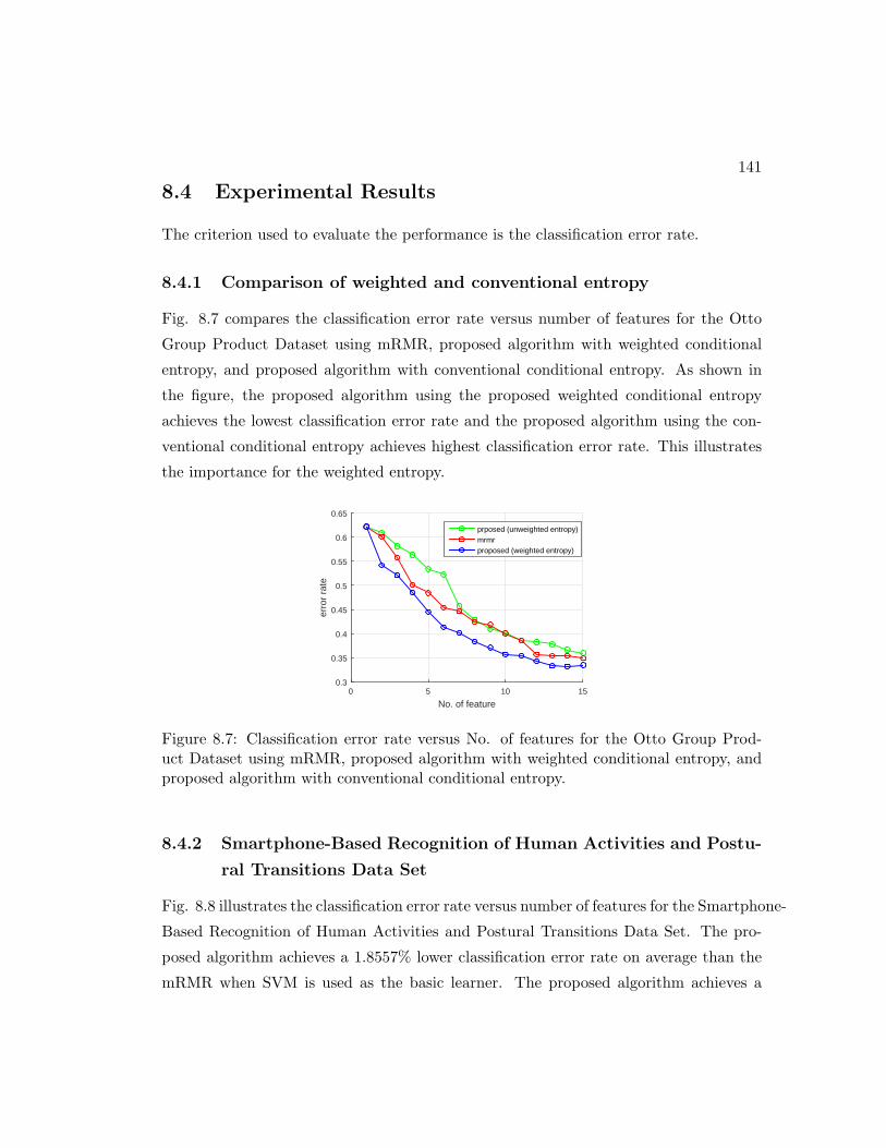
141
8.4 Experimental Results
The criterion used to evaluate the performance is the classification error rate.
8.4.1 Comparison of weighted and conventional entropy
Fig. 8.7 compares the classification error rate versus number of features for the Otto
Group Product Dataset using mRMR, proposed algorithm with weighted conditional
entropy, and proposed algorithm with conventional conditional entropy. As shown in
the figure, the proposed algorithm using the proposed weighted conditional entropy
achieves the lowest classification error rate and the proposed algorithm using the con-
ventional conditional entropy achieves highest classification error rate. This illustrates
the importance for the weighted entropy.
No. of feature0 5 10 15
erro
r ra
te
0.3
0.35
0.4
0.45
0.5
0.55
0.6
0.65
prposed (unweighted entropy)mrmrproposed (weighted entropy)
Figure 8.7: Classification error rate versus No. of features for the Otto Group Prod-uct Dataset using mRMR, proposed algorithm with weighted conditional entropy, andproposed algorithm with conventional conditional entropy.
8.4.2 Smartphone-Based Recognition of Human Activities and Postu-
ral Transitions Data Set
Fig. 8.8 illustrates the classification error rate versus number of features for the Smartphone-
Based Recognition of Human Activities and Postural Transitions Data Set. The pro-
posed algorithm achieves a 1.8557% lower classification error rate on average than the
mRMR when SVM is used as the basic learner. The proposed algorithm achieves a
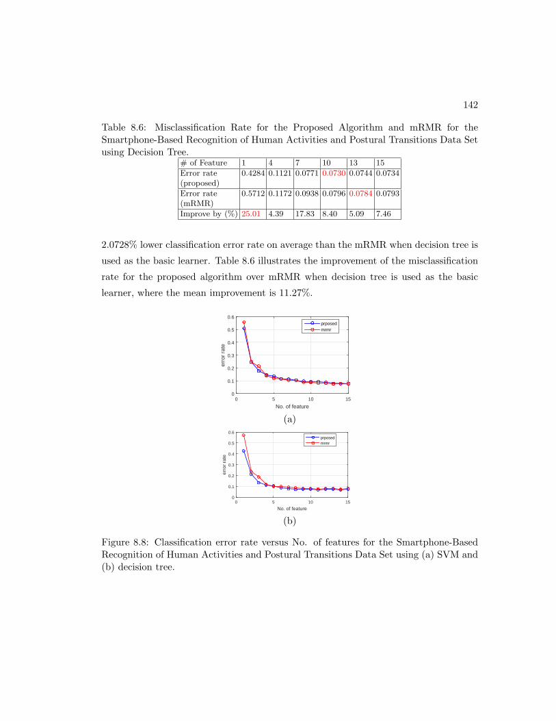
142
Table 8.6: Misclassification Rate for the Proposed Algorithm and mRMR for theSmartphone-Based Recognition of Human Activities and Postural Transitions Data Setusing Decision Tree.
# of Feature 1 4 7 10 13 15
Error rate 0.4284 0.1121 0.0771 0.0730 0.0744 0.0734(proposed)
Error rate 0.5712 0.1172 0.0938 0.0796 0.0784 0.0793(mRMR)
Improve by (%) 25.01 4.39 17.83 8.40 5.09 7.46
2.0728% lower classification error rate on average than the mRMR when decision tree is
used as the basic learner. Table 8.6 illustrates the improvement of the misclassification
rate for the proposed algorithm over mRMR when decision tree is used as the basic
learner, where the mean improvement is 11.27%.
No. of feature0 5 10 15
erro
r ra
te
0
0.1
0.2
0.3
0.4
0.5
0.6prposedmrmr
(a)
No. of feature0 5 10 15
erro
r ra
te
0
0.1
0.2
0.3
0.4
0.5
0.6prposedmrmr
(b)
Figure 8.8: Classification error rate versus No. of features for the Smartphone-BasedRecognition of Human Activities and Postural Transitions Data Set using (a) SVM and(b) decision tree.

143
8.4.3 Sensorless Drive Diagnosis Data Set
Fig. 8.9 illustrates the classification error rate versus number of features for the Sen-
sorless Drive Diagnosis Data Set. The proposed algorithm achieves a 1.5640% lower
classification error rate on average than the mRMR when SVM is used as the basic
learner. The proposed algorithm achieves a 2.2091% lower classification error rate on
average than the mRMR when decision tree is used as the basic learner. Table 8.7
illustrates the improvement of the misclassification rate for the proposed algorithm over
mRMR when decision tree is used as the basic learner, where the mean improvement is
23.91%.
No. of feature0 5 10 15
erro
r ra
te
0
0.1
0.2
0.3
0.4
0.5prposedmrmr
(a)
No. of feature0 5 10 15
erro
r ra
te
0
0.1
0.2
0.3
0.4
0.5prposedmrmr
(b)
Figure 8.9: Classification error rate versus No. of features for the Sensorless DriveDiagnosis Data Set using (a) SVM and (b) decision tree.
8.4.4 Otto Group Product Dataset
Fig. 8.10 illustrates the classification error rate versus number of features for the Otto
Group Product Dataset. The proposed algorithm achieves a 3.9653% lower classification
error rate on average than the mRMR when SVM is used as the basic learner. The

144
Table 8.7: Misclassification Rate for the Proposed Algorithm and mRMR for the Sen-sorless Drive Diagnosis Data Set using Decision Tree.
# of Feature 1 4 7 10 13 15
Error rate 0.4851 0.0158 0.0193 0.0141 0.0142 0.0157(proposed)
Error rate 0.4858 0.1184 0.0158 0.0197 0.0210 0.0211(mRMR)
Improve by (%) 0.15 86.61 -21.94 28.74 32.65 25.78
proposed algorithm achieves a 3.1271% lower classification error rate on average than
the mRMR when decision tree is used as the basic learner. Table 8.8 illustrates the
improvement of the misclassification rate for the proposed algorithm over mRMR when
decision tree is used as the basic learner, where the mean improvement is 7.10%.
No. of feature0 5 10 15
erro
r ra
te
0.3
0.35
0.4
0.45
0.5
0.55
0.6
0.65prposedmrmr
(a)
No. of feature0 5 10 15
erro
r ra
te
0.3
0.4
0.5
0.6
0.7prposedmrmr
(b)
Figure 8.10: Classification error rate versus No. of features for the Otto Group ProductDataset using (a) SVM and (b) decision tree.

145
Table 8.8: Misclassification Rate for the Proposed Algorithm and mRMR for the OttoGroup Product Dataset using Decision Tree.
# of Feature 1 4 7 10 13 15
Error rate 0.6217 0.4849 0.4021 0.3567 0.3331 0.3341(proposed)
Error rate 0.6217 0.5013 0.4466 0.4003 0.3545 0.3487(mRMR)
Improve by (%) 0.0 3.2754 9.9631 10.8841 6.0138 4.1848
Table 8.9: Misclassification Rate for the Proposed Algorithm and mRMR for the ForestType Prediction Dataset using Decision Tree.
# of Feature 1 4 7 10 13 15
Error rate 0.3272 0.3522 0.1587 0.1369 0.1236 0.1112(proposed)
Error rate 0.3274 0.3192 0.3429 0.1349 0.1078 0.1013(mRMR)
Improve by (%) 0.0652 -10.3153 53.7259 -1.4661 -14.5931 -9.7342
8.4.5 Forest Type Prediction Dataset
Fig. 8.11 illustrates the classification error rate versus number of features for the Forest
Type Prediction Dataset. The proposed algorithm achieves a 2.6398% lower classifica-
tion error rate on average than the mRMR. Table 8.9 illustrates the improvement of
the misclassification rate for the proposed algorithm over mRMR when decision tree is
used as the basic learner, where the mean improvement is 5.12%.
No. of feature0 5 10 15
erro
r ra
te
0.1
0.15
0.2
0.25
0.3
0.35
0.4prposedmrmr
Figure 8.11: Classification error rate versus No. of features for the Forest Type Predic-tion Dataset using decision tree.

146
8.5 Discussion
As illustrated in the experimental results from the Smartphone-Based Recognition of
Human Activities and Postural Transitions Data Set and the Otto Group Product
Dataset, the proposed algorithm achieves constantly a lower error rate than the m-
RMR. More importantly, as illustrated in the experimental results from the Sensorless
Drive Diagnosis Data Set and the Forest Type Prediction Dataset, the proposed al-
gorithm selects critical features which lead to a significant decrease of the error rate
in much earlier iterations. The error rate for the Sensorless Drive Diagnosis Data Set
decreases significantly when 3 features are selected when the proposed algorithm and
decision tree are used, as compared to 6 features when mRMR and decision tree are
used. The error rate for the Forest Type Prediction Dataset decreases significantly
when 6 features are selected when the proposed algorithm and decision tree are used,
as compared to 9 features when mRMR and decision tree are used.
8.6 Conclusion
A new recursive feature selection method has been presented in this chapter. Our feature
selection method places more emphasis on the predictive power of each individual feature
for part of the feature samples for multiclass classification. Our algorithm ultimately
selects a feature subset such that for each feature sample, there exists a feature that has
a lower uncertainty value in the selected feature subset.The proposed algorithm achieves
better performance than mRMR as misclassification rates are lower.

References
[1] Michael J Berry and Gordon Linoff. Data mining techniques: for marketing, sales,
and customer support. John Wiley & Sons, Inc., 1997.
[2] Usama Fayyad, Gregory Piatetsky-Shapiro, and Padhraic Smyth. From data min-
ing to knowledge discovery in databases. AI magazine, 17(3):37, 1996.
[3] Pang-Ning Tan et al. Introduction to data mining. Addison-Wesley, 2005.
[4] Christopher M Bishop. Pattern recognition. Machine Learning, 128, 2006.
[5] Sergios Theodoridis and Konstantinos Koutroumbas. Pattern Recognition. Aca-
demic Press, 2008.
[6] Vladimir Cherkassky and Filip M Mulier. Learning from data: concepts, theory,
and methods, 2nd edition. Wiley-IEEE Press, 2007.
[7] Tak-Chung Fu. A review on time series data mining. Engineering Applications of
Artificial Intelligence, 24(1):164–181, 2011.
[8] Fabian Morchen. Time series feature extraction for data mining using DWT and
DFT, 2003.
[9] Eamonn Keogh, Stefano Lonardi, and Bill’Yuan-chi’ Chiu. Finding surprising
patterns in a time series database in linear time and space. In Proceedings of the
eighth ACM SIGKDD international conference on Knowledge discovery and data
mining, pages 550–556. ACM, 2002.
147

148
[10] Reza Sameni and Gari D Clifford. A review of fetal ECG signal processing; issues
and promising directions. The open pacing, electrophysiology & therapy journal,
3:4, 2010.
[11] J Willis Hurst. Naming of the waves in the ECG, with a brief account of their
genesis. Circulation, 98(18):1937–1942, 1998.
[12] Saeid Sanei and Jonathon A Chambers. EEG signal processing. John Wiley &
Sons, 2013.
[13] Deon Garrett, David A Peterson, Charles W Anderson, and Michael H Thaut.
Comparison of linear, nonlinear, and feature selection methods for eeg signal clas-
sification. IEEE Transactions on neural systems and rehabilitation engineering,
11(2):141–144, 2003.
[14] Christian Pfister. Monthly temperature and precipitation in central europe from
1525–1979: quantifying documentary evidence on weather and its effects. Climate
since AD, 1500:118–142, 1992.
[15] Robert Loudon and Raymond LH Murphy Jr. Lung sounds 1, 2. American Review
of Respiratory Disease, 130(4):663–673, 1984.
[16] Kyoung-Jae Kim and Ingoo Han. Genetic algorithms approach to feature dis-
cretization in artificial neural networks for the prediction of stock price index.
Expert systems with Applications, 19(2):125–132, 2000.
[17] Piero Perucca, Francois Dubeau, and Jean Gotman. Intracranial electroencephalo-
graphic seizure-onset patterns: effect of underlying pathology. Brain, 137(1):183–
196, 2014.
[18] Florian Mormann, Thomas Kreuz, Christoph Rieke, Ralph G Andrzejak, Alexan-
der Kraskov, Peter David, Christian E Elger, and Klaus Lehnertz. On the pre-
dictability of epileptic seizures. Clin Neurophysiol, 116(3):569–587, 2005.
[19] Herbert Witte, Leon D Iasemidis, and Brian Litt. Special issue on epileptic seizure
prediction. IEEE Trans. Biomed. Eng., 50(5):537–539, 2003.

149
[20] Florian Mormann, Ralph G Andrzejak, Christian E Elger, and Klaus Lehnertz.
Seizure prediction: the long and winding road. Brain, 130(2):314–333, 2007.
[21] Brian Litt and Javier Echauz. Prediction of epileptic seizures. Lancet Neurol,
1(1):22–30, 2002.
[22] Yun Park, Lan Luo, Keshab K Parhi, and Theoden Netoff. Seizure prediction with
spectral power of EEG using cost-sensitive support vector machines. Epilepsia,
52(10):1761–1770, 2011.
[23] Gonzalo Alarcon, Colin Binnie, Robert Elwes, and Charles Polkey. Power spec-
trum and intracranial EEG patterns at seizure onset in partial epilepsy. Elec-
troencephalogr Clin Neurophysiol, 94(5):326–337, 1995.
[24] Patrick Celka and Paul Colditz. A computer-aided detection of EEG seizures in
infants: a singular-spectrum approach and performance comparison. IEEE Trans.
Biomed. Eng., 49(5):455–462, 2002.
[25] Florian Mormann, Klaus Lehnertz, Peter David, and Christian E Elger. Mean
phase coherence as a measure for phase synchronization and its application to the
EEG of epilepsy patients. Physica D, 144(3):358–369, 2000.
[26] ME Saab and Jean Gotman. A system to detect the onset of epileptic seizures in
scalp EEG. Clin Neurophysiol, 116(2):427–442, 2005.
[27] Zisheng Zhang and Keshab K Parhi. Low-complexity seizure prediction from
iEEG/sEEG using spectral power and ratios of spectral power. IEEE Transactions
on Biomedical Circuits and Systems, 10(3):693–706, 2016.
[28] Mojtaba Bandarabadi, Cesar A Teixeira, Jalil Rasekhi, and Antonio Dourado.
Epileptic seizure prediction using relative spectral power features. Clin Neuro-
physiol, 2014.
[29] Zisheng Zhang and Keshab K Parhi. Seizure detection using regression tree based
feature selection and polynomial SVM classification. Conf. Proc. IEEE Eng. Med.
Biol. Soc., 2015.

150
[30] Mojtaba Bandarabadi, Cesar Teixeira, Tay Netoff, Keshab K Parhi, and Antonio
Dourado. Robust and low complexity algorithms for seizure detection. Conf. Proc.
IEEE Eng. Med. Biol. Soc., 2014.
[31] Zisheng Zhang and Keshab K Parhi. Seizure detection using wavelet decompo-
sition of the prediction error signal from a single channel of intra-cranial EEG.
In 2014 36th Annual International Conference of the IEEE on Engineering in
Medicine and Biology Society (EMBC), pages 4443–4446. IEEE, 2014.
[32] Nitish V Thakor and Y-S Zhu. Applications of adaptive filtering to ECG analysis:
noise cancellation and arrhythmia detection. IEEE transactions on biomedical
engineering, 38(8):785–794, 1991.
[33] H Altay Guvenir, Burak Acar, Gulsen Demiroz, and Ayhan Cekin. A supervised
machine learning algorithm for arrhythmia analysis. In Computers in Cardiology
1997, pages 433–436. IEEE, 1997.
[34] Fabian Paschke, Christian Bayer, Martyna Bator, Uwe Monks, Alexander Dick-
s, Olaf Enge-Rosenblatt, and Volker Lohweg. Sensorlose zustandsuberwachung
an synchronmotoren. In Proceedings. 23. Workshop Computational Intelligence,
Dortmund, 5.-6. Dezember 2013, page 211. KIT Scientific Publishing, 2013.
[35] M. Lichman. UCI machine learning repository, 2013.
[36] Tingting Xu, Massoud Stephane, and Keshab K Parhi. Abnormal neural oscil-
lations in schizophrenia assessed by spectral power ratio of MEG during word
processing. IEEE Transactions on Neural Systems and Rehabilitation Engineer-
ing, 24(11):1148–1158, 2016.
[37] Gareth James, Daniela Witten, Trevor Hastie, and Robert Tibshirani. An intro-
duction to statistical learning, volume 6. Springer, 2013.
[38] Isabelle Guyon and Andre Elisseeff. An introduction to variable and feature se-
lection. Journal of machine learning research, 3(Mar):1157–1182, 2003.
[39] Huan Liu and Hiroshi Motoda. Feature selection for knowledge discovery and data
mining, volume 454. Springer Science & Business Media, 2012.

151
[40] Lei Yu and Huan Liu. Efficient feature selection via analysis of relevance and
redundancy. Journal of machine learning research, 5(Oct):1205–1224, 2004.
[41] Ian Jolliffe. Principal component analysis. Wiley Online Library, 2002.
[42] Khalid Sayood. Introduction to data compression. Morgan Kaufmann, 2012.
[43] De Wang, Feiping Nie, and Heng Huang. Feature selection via global redun-
dancy minimization. IEEE Transactions on Knowledge and Data Engineering,
27(10):2743–2755, 2015.
[44] Huan Liu and Lei Yu. Toward integrating feature selection algorithms for clas-
sification and clustering. IEEE Transactions on knowledge and data engineering,
17(4):491–502, 2005.
[45] Yuexian Hou, Peng Zhang, Tingxu Yan, Wenjie Li, and Dawei Song. Beyond
redundancies: A metric-invariant method for unsupervised feature selection. IEEE
Transactions on Knowledge and Data Engineering, 22(3):348–364, 2010.
[46] Mairead L Bermingham, Ricardo Pong-Wong, Athina Spiliopoulou, Caroline Hay-
ward, Igor Rudan, Harry Campbell, Alan F Wright, James F Wilson, Felix A-
gakov, Pau Navarro, and Chris S Haley. Application of high-dimensional feature
selection: evaluation for genomic prediction in man. Scientific reports, 5:10312,
2015.
[47] Howard C Choe, Yulun Wan, and Andrew K Chan. Neural pattern identification
of railroad wheel-bearing faults from audible acoustic signals: Comparison of FFT,
CWT, and DWT features. In AeroSense’97, pages 480–496. International Society
for Optics and Photonics, 1997.
[48] Norden E Huang, Zheng Shen, Steven R Long, Manli CWu, Hsing H Shih, Quanan
Zheng, Nai-Chyuan Yen, Chi Chao Tung, and Henry H Liu. The empirical mode
decomposition and the Hilbert spectrum for nonlinear and non-stationary time
series analysis. In Proceedings of the Royal Society of London A: Mathematical,
Physical and Engineering Sciences, volume 454, pages 903–995. The Royal Society,
1998.

152
[49] Larry S Shapiro and J Michael Brady. Feature-based correspondence: an eigen-
vector approach. Image and vision computing, 10(5):283–288, 1992.
[50] Luigi Chisci, Antonio Mavino, Guido Perferi, Marco Sciandrone, Carmelo Anile,
Gabriella Colicchio, and Filomena Fuggetta. Real-time epileptic seizure predic-
tion using AR models and support vector machines. IEEE Trans. Biomed. Eng.,
57(5):1124–1132, 2010.
[51] Cesar Alexandre Teixeira, Bruno Direito, Mojtaba Bandarabadi, Michel
Le Van Quyen, Mario Valderrama, Bjoern Schelter, Andreas Schulze-Bonhage,
Vincent Navarro, Francisco Sales, and Antonio Dourado. Epileptic seizure predic-
tors based on computational intelligence techniques: A comparative study with
278 patients. Comput Methods Programs Biomed, 114(3):324–336, 2014.
[52] Ning Wang and Michael R Lyu. Extracting and selecting distinctive EEG features
for efficient epileptic seizure prediction. IEEE journal of biomedical and health
informatics, 19(5):1648–1659, 2015.
[53] Ali Hossam Shoeb. Application of machine learning to epileptic seizure onset
detection and treatment. PhD thesis, Massachusetts Institute of Technology, 2009.
[54] Ary L Goldberger, Luis AN Amaral, Leon Glass, Jeffrey M Hausdorff,
Plamen Ch Ivanov, Roger G Mark, Joseph E Mietus, George B Moody,
Chung-Kang. Peng, and H Eugene Stanley. PhysioBank, PhysioToolkit, and
PhysioNet: Components of a new research resource for complex physio-
logic signals. Circulation, 101(23):e215–e220, 2000. Circulation Electronic
Pages: http://circ.ahajournals.org/cgi/content/full/101/23/e215 PMID:1085218;
doi: 10.1161/01.CIR.101.23.e215.
[55] Keshab K Parhi and Zisheng Zhang. Seizure prediction using ratio of spectral
power from single EEG electrode. Proc. of 6th International Workshop on Seizure
Prediction (IWSP6), page 39, 2013.
[56] Stephane Mallat. A wavelet tour of signal processing: the sparse way. Academic
Press, 2008.

153
[57] Yiming Yang and Jan O Pedersen. A comparative study on feature selection in
text categorization. In ICML, volume 97, pages 412–420, 1997.
[58] Pierre A Devijver and Josef Kittler. Pattern recognition: A statistical approach.
Prentice hall, 1982.
[59] Pradipta Maji and Sankar K Pal. Feature selection using f-information measures
in fuzzy approximation spaces. IEEE Transactions on Knowledge and Data En-
gineering, 22(6):854–867, 2010.
[60] Shuang Hong Yang and Bao-Gang Hu. Discriminative feature selection by non-
parametric bayes error minimization. IEEE Transactions on knowledge and data
engineering, 24(8):1422–1434, 2012.
[61] Hubert W Lilliefors. On the Kolmogorov-Smirnov test for normality with
mean and variance unknown. Journal of the American Statistical Association,
62(318):399–402, 1967.
[62] Mark A Hall. Correlation-based feature selection of discrete and numeric class
machine learning. In Proceedings of the 17th International Conference on Machine
Learning, pages 359–366, 2000.
[63] Thomas M Cover and Joy A Thomas. Elements of information theory. John
Wiley & Sons, 2012.
[64] George Forman. An extensive empirical study of feature selection metrics for text
classification. Journal of machine learning research, 3(Mar):1289–1305, 2003.
[65] Guangzhi Qu, Salim Hariri, and Mazin Yousif. A new dependency and correlation
analysis for features. IEEE Transactions on Knowledge and Data Engineering,
17(9):1199–1207, 2005.
[66] Norbert Henze and Mathew D Penrose. On the multivariate runs test. Annals of
statistics, pages 290–298, 1999.
[67] Manoranjan Dash and Huan Liu. Consistency-based search in feature selection.
Artificial intelligence, 151(1):155–176, 2003.

154
[68] Ron Kohavi and George H John. Wrappers for feature subset selection. Artificial
intelligence, 97(1):273–324, 1997.
[69] Pat Langley. Selection of relevant features in machine learning. In Proceedings of
the AAAI Fall symposium on relevance, volume 184, pages 245–271, 1994.
[70] Richard O Duda, Peter E Hart, and David G Stork. Pattern classification. John
Wiley & Sons, 2012.
[71] Petr Somol, Pavel Pudil, and Josef Kittler. Fast branch & bound algorithms for
optimal feature selection. IEEE Transactions on Pattern Analysis and Machine
Intelligence, 26(7):900–912, 2004.
[72] Wojciech Siedlecki and Jack Sklansky. On automatic feature selection. Interna-
tional Journal of Pattern Recognition and Artificial Intelligence, 2(02):197–220,
1988.
[73] Pavel Pudil, Jana Novovicova, and Josef Kittler. Floating search methods in
feature selection. Pattern recognition letters, 15(11):1119–1125, 1994.
[74] Isabelle Guyon, Jason Weston, Stephen Barnhill, and Vladimir Vapnik. Gene
selection for cancer classification using support vector machines. Machine learning,
46(1-3):389–422, 2002.
[75] Jason Weston, Andre Elisseeff, Bernhard Scholkopf, and Mike Tipping. Use of the
zero-norm with linear models and kernel methods. Journal of machine learning
research, 3(Mar):1439–1461, 2003.
[76] Jason Weston, Sayan Mukherjee, Olivier Chapelle, Massimiliano Pontil, Tomaso
Poggio, and Vladimir Vapnik. Feature selection for SVMs. Advances in neural
information processing systems, 2000.
[77] Yi-Wei Chen and Chih-Jen Lin. Combining svms with various feature selection
strategies. Feature Extraction, pages 315–324, 2006.
[78] Vinay Kariwala, Lingjian Ye, and Yi Cao. Branch and bound method for
regression-based controlled variable selection. Comput Chem Eng, 54:1–7, 2013.

155
[79] Robert Tibshirani. Regression shrinkage and selection via the lasso. Journal of
the Royal Statistical Society. Series B (Methodological), pages 267–288, 1996.
[80] Leo Breiman, Jerome Friedman, Charles J Stone, and Richard A Olshen. Classi-
fication and regression trees. CRC press, 1984.
[81] Zisheng Zhang and Keshab K Parhi. Seizure prediction using polynomial SVM
classification. Conf. Proc. IEEE Eng. Med. Biol. Soc., 2015.
[82] Roberto Battiti. Using mutual information for selecting features in supervised
neural net learning. IEEE Transactions on neural networks, 5(4):537–550, 1994.
[83] Hanchuan Peng, Fuhui Long, and Chris Ding. Feature selection based on mutu-
al information criteria of max-dependency, max-relevance, and min-redundancy.
IEEE Transactions on pattern analysis and machine intelligence, 27(8):1226–1238,
2005.
[84] Howard Hua Yang and John E Moody. Data visualization and feature selection:
New algorithms for nongaussian data. In NIPS, volume 99, pages 687–693. Cite-
seer, 1999.
[85] Nojun Kwak and Chong-Ho Choi. Input feature selection for classification prob-
lems. IEEE Transactions on Neural Networks, 13(1):143–159, 2002.
[86] Dahua Lin and Xiaoou Tang. Conditional infomax learning: an integrated frame-
work for feature extraction and fusion. In European Conference on Computer
Vision, pages 68–82. Springer, 2006.
[87] Francois Fleuret. Fast binary feature selection with conditional mutual informa-
tion. Journal of Machine Learning Research, 5(Nov):1531–1555, 2004.
[88] Michel Vidal-Naquet and Shimon Ullman. Object recognition with informative
features and linear classification. In ICCV, volume 3, page 281, 2003.
[89] Gavin Brown. A new perspective for information theoretic feature selection. In
AISTATS, pages 49–56, 2009.

156
[90] Jorge R Vergara and Pablo A Estevez. A review of feature selection methods based
on mutual information. Neural Computing and Applications, 24(1):175–186, 2014.
[91] Tom M Mitchell. Machine learning. 1997. Burr Ridge, IL: McGraw Hill, 45:37,
1997.
[92] Ronald A Fisher. The use of multiple measurements in taxonomic problems.
Annals of eugenics, 7(2):179–188, 1936.
[93] Yoav Freund and Robert E Schapire. Experiments with a new boosting algorithm.
In ICML, volume 96, pages 148–156, 1996.
[94] Manohar Ayinala and Keshab K Parhi. Low complexity algorithm for seizure
prediction using Adaboost. Conf. Proc. IEEE Eng. Med. Biol. Soc., pages 1061–
1064, 2012.
[95] Zisheng Zhang and Keshab K Parhi. FDMR: Frequency-domain model ratio
for identifying change of state from a single time-series. IEEE Transactions on
Biomedical Engineering, 2017 (submitted).
[96] Zisheng Zhang and Keshab K Parhi. Seizure prediction using long-term frag-
mented intracranial canine and human EEG recordings. In 2016 50th Asilomar
Conference on Signals, Systems and Computers, pages 361–365. IEEE, 2016.
[97] Manohar Ayinala and Keshab K Parhi. Low-energy architectures for support vec-
tor machine computation. In Conf. Rec. Asilomar Conf. Signals. Syst. Comput.,
pages 2167–2171. IEEE, 2013.
[98] Zisheng Zhang and Keshab K Parhi. MUSE: Minimum uncertainty and sample
elimination based binary feature selection. IEEE Transactions on Knowledge and
Data Engineering, 2017 (submitted).
[99] Zisheng Zhang and Keshab K Parhi. M3U: Minimum mean minimum uncertainty
feature selection for multiclass classification. IEEE Transactions on Knowledge
and Data Engineering, 2017 (submitted).
[100] University of Freiburg. Seizure prediction project freiburg. https://epilepsy.
uni-freiburg.de/freiburg-seizure-predictionproject/eeg-database.

157
[101] Simon S Haykin. Adaptive Filter Theory, 4th edition. Prentice Hall, 2002.
[102] Ali Shoeb, Herman Edwards, Jack Connolly, Blaise Bourgeois, S Ted Treves, and
John Guttag. Patient-specific seizure onset detection. Epilepsy Behav, 5(4):483–
498, 2004.
[103] Jonas Henriksen, Line Sofie Remvig, Rasmus Elsborg Madsen, Isa Conradsen,
Troels Wesenberg Kjær, Carsten Eckhart Thomsen, and Helge BD Sorensen. Au-
tomatic seizure detection: going from sEEG to iEEG. In Conf. Proc. IEEE Eng.
Med. Biol. Soc., pages 2431–2434. IEEE, 2010.
[104] Ardalan Aarabi, Reza Fazel-Rezai, and Yahya Aghakhani. A fuzzy rule-based
system for epileptic seizure detection in intracranial EEG. Clin Neurophysiol,
120(9):1648–1657, 2009.
[105] Lalit M Patnaik and Ohil K Manyam. Epileptic EEG detection using neural
networks and post-classification. Comput Meth Prog Bio, 91(2):100–109, 2008.
[106] Hao Qu and Jean Gotman. A patient-specific algorithm for the detection of seizure
onset in long-term EEGmonitoring: possible use as a warning device. IEEE Trans.
Biomed. Eng., 44(2):115–122, 1997.
[107] G Udny Yule. On a method of investigating periodicities in disturbed series,
with special reference to Wolfer’s sunspot numbers. Philosophical Transactions of
the Royal Society of London. Series A, Containing Papers of a Mathematical or
Physical Character, 226:267–298, 1927.
[108] Jin Huang and Charles X Ling. Using AUC and accuracy in evaluating learning
algorithms. IEEE Transactions on knowledge and Data Engineering, 17(3):299–
310, 2005.
[109] Charles X Ling, Jin Huang, and Harry Zhang. AUC: a statistically consistent and
more discriminating measure than accuracy. In IJCAI, volume 3, pages 519–524,
2003.
[110] National Institues of Health and American Epilepsy Society. Upenn and mayo clin-
ic’s seizure detection challenge. urlhttps://www.kaggle.com/c/seizure-detection.

158
[111] Lisa D Coles, Edward E Patterson, W Douglas Sheffield, Jaideep Mavoori, Jason
Higgins, Bland Michael, Kent Leyde, James C Cloyd, Brian Litt, and Charles Vite.
Feasibility study of a caregiver seizure alert system in canine epilepsy. Epilepsy
research, 106(3):456–460, 2013.
[112] Matt Stead, Mark Bower, Benjamin H Brinkmann, Kendall Lee, W Richard
Marsh, Fredric B Meyer, Brian Litt, Jamie Van Gompel, and Greg A Worrell.
Microseizures and the spatiotemporal scales of human partial epilepsy. Brain,
page awq190, 2010.
[113] Varun Bajaj and Ram Bilas Pachori. Epileptic seizure detection based on the
instantaneous area of analytic intrinsic mode functions of EEG signals. Biomed
Eng Lett, 3(1):17–21, 2013.
[114] Qi Yuan, Weidong Zhou, Yinxia Liu, and Jiwen Wang. Epileptic seizure detection
with linear and nonlinear features. Epilepsy & Behavior, 24(4):415–421, 2012.
[115] Jasmin Kevric and Abdulhamit Subasi. The effect of multiscale PCA de-noising
in epileptic seizure detection. J Med Syst, 38(10):1–13, 2014.
[116] Jose Leon-Carrion, Juan Francisco Martin-Rodriguez, Jesus Damas-Lopez,
Juan Manuel Barroso y Martin, and Maria Rosario Dominguez-Morales. Delta–
alpha ratio correlates with level of recovery after neurorehabilitation in patients
with acquired brain injury. Clin Neurophysiol, 120(6):1039–1045, 2009.
[117] Jan Claassen, Lawrence J Hirsch, Kurt T Kreiter, Evelyn Y Du, E Sander Con-
nolly, Ronald G Emerson, and Stephan A Mayer. Quantitative continuous EEG
for detecting delayed cerebral ischemia in patients with poor-grade subarachnoid
hemorrhage. Clin neurophysiol, 115(12):2699–2710, 2004.
[118] Corinna Cortes and Vladimir Vapnik. Support-vector networks. Mach Learn,
20(3):273–297, 1995.
[119] Yi Lin, Yoonkyung Lee, and Grace Wahba. Support vector machines for classifi-
cation in nonstandard situations. Mach Learn, 46(1-3):191–202, 2002.

159
[120] Aravinth Chinnapalanichamy and Keshab K Parhi. Serial and interleaved archi-
tectures for computing real FFT. In Proc. IEEE Int. Conf. Acoust. Speech Signal
Process. IEEE, 2015.
[121] Thomas Maiwald, Matthias Winterhalder, Richard Aschenbrenner-Scheibe, Hen-
ning U Voss, Andreas Schulze-Bonhage, and Jens Timmer. Comparison of three
nonlinear seizure prediction methods by means of the seizure prediction charac-
teristic. Physica D, 194(3):357–368, 2004.
[122] James R Williamson, Daniel W Bliss, and David W Browne. Epileptic seizure
prediction using the spatiotemporal correlation structure of intracranial EEG.
Proc. IEEE Int. Conf. Acoust. Speech Signal Process, pages 665–668, 2011.
[123] Richard Aschenbrenner-Scheibe, Thomas Maiwald, Matthias Winterhalder, Hen-
ning U Voss, Jens Timmer, and Andreas Schulze-Bonhage. How well can epileptic
seizures be predicted? an evaluation of a nonlinear method. Brain, 126(12):2616–
2626, 2003.
[124] Yang Zheng, Gang Wang, Kuo Li, Gang Bao, and Jue Wang. Epileptic seizure
prediction using phase synchronization based on bivariate empirical mode decom-
position. Clin Neurophysiol, 125(6):1104–1111, 2013.
[125] Nilufer Ozdemir and Esen Yildirim. Patient specific seizure prediction system
using hilbert spectrum and bayesian networks classifiers. Comput Math Methods
Med, 2014, 2014.
[126] Ardalan Aarabi and Bin He. Seizure prediction in hippocampal and neocortical
epilepsy using a model-based approach. Clin Neurophysiol, 125(5):930–940, 2014.
[127] Hedi Khammari and Ashraf Anwar. A spectral based forecasting tool of epileptic
seizures. IJCSI International Journal of Computer, 2012.
[128] Kai-Quan Shen, Chong-Jin Ong, Xiao-Ping Li, Zheng Hui, and E Wilder-Smith.
A feature selection method for multilevel mental fatigue EEG classification. IEEE
Trans. Biomed. Eng., 54(7):1231–1237, 2007.

160
[129] Kaggle. American epilepsy society seizure prediction challenge. https://www.
kaggle.com/c/seizure-prediction.
[130] J Jeffry Howbert, Edward E Patterson, S Matt Stead, Ben Brinkmann, Vincent
Vasoli, Daniel Crepeau, Charles H Vite, Beverly Sturges, Vanessa Ruedebusch,
Jaideep Mavoori, Kent Leyde, W. Douglas Sheffield, Brian Litt, and Gregory A.
Worrell. Forecasting seizures in dogs with naturally occurring epilepsy. PLoS One,
9(1):e81920, 2014.
[131] Mark J Cook, Terence J O’Brien, Samuel F Berkovic, Michael Murphy, An-
drew Morokoff, Gavin Fabinyi, Wendyl D’Souza, Raju Yerra, John Archer, Lu-
cas Litewka, et al. Prediction of seizure likelihood with a long-term, implanted
seizure advisory system in patients with drug-resistant epilepsy: a first-in-man
study. Lancet Neurol, 12(6):563–571, 2013.
[132] Yin Liu, Hariharasudhan Venkataraman, Zisheng Zhang, and Keshab K Parhi.
Machine learning classifiers using stochastic logic. In Proc. of IEEE 34th Inter-
national Conference on Computer Design (ICCD), pages 408–411. IEEE, 2016.
[133] UCI. Multiple features data set. http://archive.ics.uci.edu/ml/datasets/
Multiple+Features.
[134] Anil K Jain, Robert P. W. Duin, and Jianchang Mao. Statistical pattern recogni-
tion: A review. IEEE Transactions on pattern analysis and machine intelligence,
22(1):4–37, 2000.
[135] Anil Jain and Douglas Zongker. Feature selection: Evaluation, application, and
small sample performance. IEEE transactions on pattern analysis and machine
intelligence, 19(2):153–158, 1997.
[136] Robert PW Duin and David MJ Tax. Experiments with classifier combining rules.
In International Workshop on Multiple Classifier Systems, pages 16–29. Springer,
2000.
[137] UCI. Arrhythmia data set. https://archive.ics.uci.edu/ml/datasets/
Arrhythmia.

161
[138] Shay Cohen, Eytan Ruppin, and Gideon Dror. Feature selection based on the
shapley value. IJCAI, pages 665–670, 2005.
[139] Gisele L Pappa, Alex A Freitas, and Celso AA Kaestner. A multiobjective genetic
algorithm for attribute selection. In Proc. 4th Int. Conf. on Recent Advances
in Soft Computing (RASC-2002), pages 116–121. Nottingham Trent University,
2002.
[140] UCI. Gisette data set. https://archive.ics.uci.edu/ml/datasets/Gisette.
[141] Isabelle Guyon, Steve Gunn, Asa Ben-Hur, and Gideon Dror. Result analysis
of the nips 2003 feature selection challenge. In Advances in neural information
processing systems, pages 545–552, 2004.
[142] Isabelle Guyon, Steve Gunn, Masoud Nikravesh, and Lofti Zadeh. Fea-
ture extraction, foundations and applications. Studies in Fuzziness and Soft
ComputingSpringer-Verlag, pages 315–324, 2006.
[143] Benjamin H Brinkmann, Joost Wagenaar, Drew Abbot, Phillip Adkins, Simone C
Bosshard, Min Chen, Quang M Tieng, Jialune He, FJ Munoz-Almaraz, Paloma
Botella-Rocamora, et al. Crowdsourcing reproducible seizure forecasting in human
and canine epilepsy. Brain, 139(6):1713–1722, 2016.
[144] Thomas G. Dietterich and Ghulum Bakiri. Solving multiclass learning problems
via error-correcting output codes. Journal of artificial intelligence research, 2:263–
286, 1995.
[145] Erin L Allwein, Robert E Schapire, and Yoram Singer. Reducing multiclass to
binary: A unifying approach for margin classifiers. Journal of machine learning
research, 1(Dec):113–141, 2000.
[146] Otto Group. Otto group product classification challenge. https://www.kaggle.
com/, 2014.

162
[147] Jorge-Luis Reyes-Ortiz, Luca Oneto, Alessandro Ghio, Albert Sama, Davide An-
guita, and Xavier Parra. Human activity recognition on smartphones with aware-
ness of basic activities and postural transitions. In International Conference on
Artificial Neural Networks, pages 177–184. Springer, 2014.
[148] Davide Anguita, Alessandro Ghio, Luca Oneto, Xavier Parra, and Jorge Luis
Reyes-Ortiz. A public domain dataset for human activity recognition using s-
martphones. In ESANN, 2013.
[149] Jorge-L Reyes-Ortiz, Luca Oneto, Albert Sama, Xavier Parra, and Davide Angui-
ta. Transition-aware human activity recognition using smartphones. Neurocom-
puting, 171:754–767, 2016.
[150] UCI. Forest cover type prediction. https://www.kaggle.com/, 2014.