missing-feature approaches in speech recognition drobust/papers/rajstern_spmag.pdf · mathematics...

1053-5888/05/$20.00©2005IEEE IEEE SIGNAL PROCESSING MAGAZINE [101] SEPTEMBER 2005

© ARTVILLE & COMSTOCK

Despite decades of focused research on the problem, the accuracy of automatic speech recog-nition (ASR) systems is still adversely affected by noise and other sources of acoustical vari-ability. For example, there are presently dozens, if not hundreds, of algorithms that havebeen developed to cope with the effects of quasistationary additive noise and linear filteringof the channel [16], [23]. While these approaches are reasonably effective in the context of

their intended purposes, they are generally ineffective in improving recognition accuracy in many moredifficult environments. Some of these more challenging conditions, which are frequently encountered insome of the most important potential speech recognition applications today, include speech in the pres-ence of transient and nonstationary disturbances (as in many factory, military, and telematic environ-ments), speech in the presence of background music or background speech (as in the automatictranscription of broadcast program material as well as in many natural environments), and speech at verylow signal-to-noise ratios (SNRs).

Conventional environmental compensation provides only limited benefit for these problems even today.For example, Raj et al. [29] showed that while codeword-dependent cepstral normalization is highly effectivein dramatically reducing the impact of additive broadband noise on speech recognition accuracy, it is rela-tively ineffective when speech is presented to the system in the presence of background music, for reasonsthat are believed to be a consequence of the nonstationary nature of the acoustical degradation.

[Bhiksha Raj and Richard M. Stern]

Missing-Feature Approaches inSpeech Recognition

[Improving recognition accuracy in

noise by using partial spectrographic

information]

IEEE SIGNAL PROCESSING MAGAZINE [102] SEPTEMBER 2005

This article describes and discusses alternative robust recog-nition approaches that have come to be known as missing fea-ture approaches [9], [10], [20]. These approaches are based onthe observation that speech signals have a high degree of redun-dancy—human listeners are able to comprehend speech that hasundergone considerable spectral excisions. For example, normalconversation is possible with speech that has been either high- orlow-pass filtered with a cutoff frequency of 1,800 Hz [17].

Briefly, in missing feature approaches, one attempts to deter-mine which cells of a spectrogram-like time-frequency display ofspeech information are unreliable (or missing) because of degra-dation due to noise or to other types of interference. The cellsthat are determined to be unreliable or missing are eitherignored in subsequent processing and statistical analysis(although they may provide ancillary information), or they arefilled in by optimal estimation of their putative values.

The application of missing feature techniques to robust auto-matic speech recognition has been strongly influenced by twocomplementary fields of signal analysis. Many of the mathemati-cal approaches to missing feature recognition were first devel-oped for the task of completing partially occluded objects in

visual pattern recognition [1]. In addition, there is a stronginterchange of techniques and applications between missing fea-ture recognition and the field of computational auditory sceneanalysis (CASA), which seeks to segregate, identify, and recog-nize the separate components of a complex sound field [8]. Themathematics developed for missing feature recognition can beapplied to other types of signal restoration implicit in CASA, andthe analysis approaches developed in CASA can be useful foridentifying degraded components of signals that can potentiallybe restored through the use of missing feature techniques.

SPECTRAL MEASUREMENTS AND SPECTROGRAPHIC MASKSMissing feature methods model the effect of noise on speech asthe corruption of regions of time-frequency representations ofthe speech signal. A variety of time-frequency representationsmay be used for the purpose. Most of them follow the same basicprocedure: the speech signal is first segmented into overlapping

frames, typically about 25 ms wide. From each frame, a powerspectrum is estimated as

Zp(m, k) =∣∣∣∣∣

N−1∑

n= 0

w(n − mL)x(n)e− j2π(n−mL)k/N

∣∣∣∣∣

2

, (1)

where Zp(m, k) represents the k th frequency band of the powerspectrum of the m th frame of speech, w(n) represents a win-dow function, x(n) represents the n th sample of the speech sig-nal, L represents the shift in samples between adjacent frames,and N represents the number of samples within the segment.The power spectral components are often reduced to a smallernumber of components using triangular weighting functionsthat represent the frequency responses of the filters in a filterbank that is designed to mimic the frequency sensitivity of thehuman ear

Xp(m, k) =∑

j

hk( j)Zp(m, j), (2)

where hk( j) represents thefrequency response of thek th filter in the filter bank.The most commonly usedfilter banks are the Mel fil-ter bank [13] and the ERBfilter bank [21].Alternately, Xp(m, k) maybe obtained by samplingthe envelope of signals atthe output of a filter bank[25]. We will refer to boththe power spectra given by(1) and the combinedpower spectra of (2) gener-ically as power spectra.

The power spectral components are compressed by a nonlin-ear function to obtain the final time-frequency representation,X(m, k) = f(Xp(m, k)), where f(·) is usually a logarithm or acube root. We assume, without loss of generality, that f(·) is alogarithm. The outcome of the analysis is a two-dimensionalrepresentation of the speech signal, which we will refer to as aspectrogram. Figure 1(a) shows a pictorial representation ofthe spectrogram for a clean speech signal.

When the speech signal is corrupted by uncorrelated additivenoise, the power spectrum of the resulting signal is the sum ofthe power spectra of the clean speech and the noise

Yp(m, k) = Xp(m, k) + Np(m, k), (3)

where Yp(m, k) and Np(m, k) represent the k th frequencybands of the power spectrum of the noisy speech and the noise,respectively, in the m th frame of the signal. Since all power

[FIG1] (a) The “mel’’ spectrogram for an utterance of clean speech. (b) The mel spectrogram for the sameutterance when it has been corrupted by white noise to an SNR of 10 dB. (c) Spectrographic mask forthe noise-corrupted utterance using an SNR threshold of 0 dB.

2

20

Time (s) Time (s) Time (s)

(a) (b) (c)

Mel

Filt

er In

dex

1816141210

864


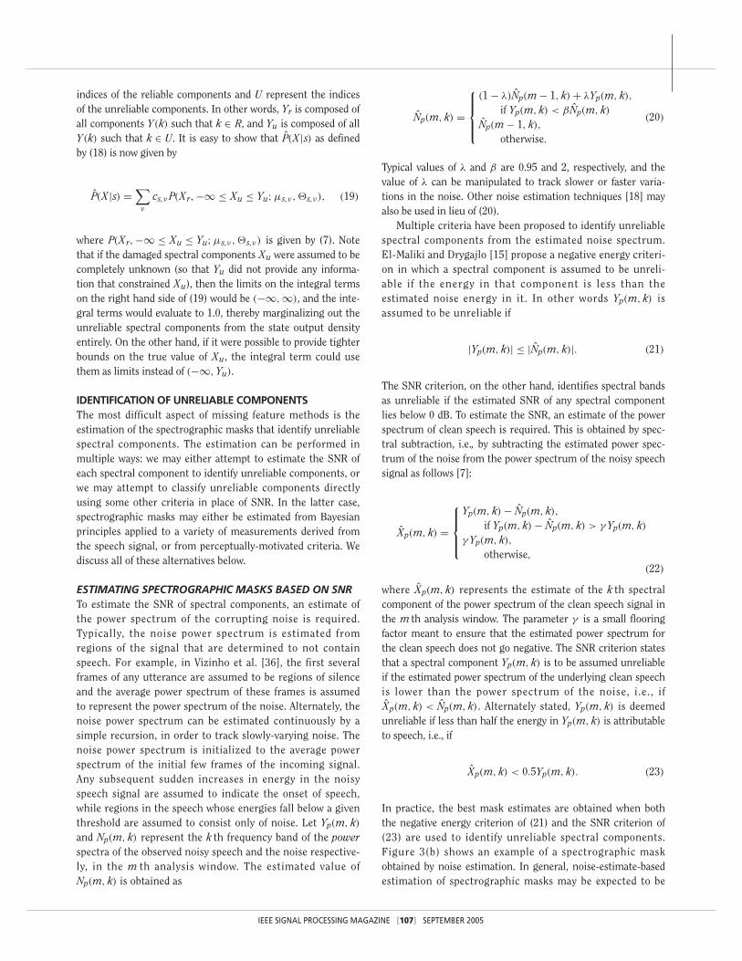
spectral terms are nonnegative, Yp(m, k) is nearly alwaysgreater than or equal to Xp(m, k). (In reality, finite-sized sam-ples of uncorrelated processes are rarely perfectly orthogonal,and the power spectra of two uncorrelated processes do not sim-ply add within any particular analysis frame. To account for this,an additional factor of 2

√Xp(m, k)Np(m, k) cos(θ) must be

included in (3), where θ is the angle between the k th term ofthe complex spectra of the speech and the noise. In practice,however, this term is usually small and can safely be ignored.)The SNR of Yp(m, k), the (m, k)th component of the spectro-gram of the noisy signal, is given by Xp(m, k)/Np(m, k). TheSNR of the spectrogram varies with both time and frequency.Typically, for any level of noise, the spectrogram includesregions of very high SNR (which are dominated by contribu-tions of the speech component), as well as regions of very lowSNR (which represent the characteristics of the noise more thanthe underlying speech). The low SNR regions of the spectro-gram adversely affect speech recognition accuracy. As the overallSNR of a noisy utterance decreases, the proportion of low SNRregions increases, resulting in worse recognition accuracy.

In missing feature methods, it is assumed that all compo-nents of a spectrogram with SNR above some threshold T arereliable estimates of the corresponding components of cleanspeech. In other words, it is assumed that the observed valueY(m, k) of such components is equal to the value X(m, k)that would have been obtained had there been no noise.Spectral components Y(m, k) with SNRs below the thresh-old, however, are assumed to be unreliable and assumed notto represent X(m, k). They merely provide an upper boundon the true value of X(m, k), i.e., X(m, k) ≤ Y(m, k). The setof tags that identify reliable and unreliable components ofthe spectrogram are referred to as the spectrographic maskfor the utterance. Recognition must now be performed withthe resulting incomplete measurements of the speech signal,where only some of the spectral components are reliablyknown and the rest are essentially unknown. Figure 1(b)shows the spectrogram for the utterance in Figure 1(a) afterit has been corrupted to 10 dB by white noise. Figure 1(c)shows the spectrographic mask for the utterance when athreshold of 0 dB is used to identify unreliable elements, withthe black regions representing the values of m and k, forwhich the corresponding spectral values Zp(m, k) are to beconsidered reliable. While in practice there is no single opti-mal threshold [28], [33], Cooke et al. and Raj et al. have typi-cally used thresholds that lie between 5 and −5 dB.

Before we proceed, we must establish some of the notationand terminology used in the rest of the article. We representthe observed power spectrum for the m th frame of speech as avector Yp(m) and the individual frequency components ofYp(m) as Yp(m, k). We assume that the final time-frequencyrepresentation consists of sequences of log-spectral vectorsderived as the logarithm of the power spectrum. We representthe m th log spectral vector as Y(m) and the individual fre-quency components in it as Y(m, k). For noisy speech signals,the observed signal is assumed to be a combination of a clean

speech signal and noise. We represent the power spectrum ofthe clean speech in the m th frame of speech as the vectorXp(m), the corresponding log-spectral vector as X(m), and theindividual frequency components of the two as Xp(m, k) andX(m, k), respectively. In addition, we represent the power spec-trum of the corresponding noise and its frequency componentsas Np(m) and Np(m, k). We represent the sequence of all spec-tral vectors Y(m) for any utterance as Y and the sequence of allcorresponding X(m) as X. For brevity, we refer to Y(m), X(m),and N(m) as spectral vectors (instead of log-spectral vectors)and to Y and X as spectrograms. We refer to the time and fre-quency indices (m, k) as a time-frequency location in the spec-trogram and the corresponding components X(m, k) andY(m, k) as the spectral components at that location.

Ideally, recognition would be performed with X, the spec-trogram for the clean speech (or with features derived from it).Unfortunately, the spectrogram X is obscured by the corrupt-ing noise, resulting in the observation of a noisy spectrogramY which differs from X. Every vector Y(m) in Y has a set ofreliable components that are good approximations to the cor-responding components of X(m). We represent the spectro-graphic mask that distinguishes reliable and unreliablecomponents of a spectrogram by S. The elements of S may beeither binary tags identifying spectral components as reliableor not with certainty, or they may be real numbers betweenzero and one that represent a measure of confidence in thereliability of the spectral components. For the rest of this sec-tion, we assume that the elements of S are binary. The spectro-graphic mask vector that identifies unreliable and reliablecomponents of a single spectral vector Y(m) is represented asS(m). We arrange the reliable components of Y(m) into a vec-tor Yr(m) and the corresponding components of X(m) into avector Xr(m). Each vector Y(m) also has a set of unreliablecomponents that provide an upper bound on the value of thecorresponding components of X(m). We arrange the unreli-able components of Y(m) into a vector Yu(m), and the corre-sponding components of X(m) into Xu(m). We refer to the setof all Yr(m) as Yr. Similarly, we refer to the set of all Yu(m),Xr(m), and Xu(m) as Yu, Xr, and Xu, respectively. The rela-tionship between Yr(m), Xr(m), Yu(m), and Xu(m) is given by

Xr(m) = Yr(m)

Xu(m) ≤ Yu(m) (4)

It is also common to assume a lower bound on Xu(m), basedon a priori knowledge of typical feature values. For instance,when the nonlinear compressive function f(·) used in the com-putation of the spectrogram is a cube root, Xu(m) is assuredlylower bounded at zero. In some sections of the article, we dropthe time and frequency-component indices of vectors, simplyrepresenting them as X, Xr, and Xu, where these vector indicesare not critical to comprehension, for brevity of notation. Thisshould not cause any confusion.


ADDITIONAL BACKGROUNDIn this section, we briefly describe three other topics that are ofrelevance to the rest of this article: speech recognition based onhidden Markov models (HMMs), bounded marginalization ofGaussian densities, and bounded maximum a posteriori estima-tion of Gaussian random variables.

SPEECH RECOGNITION USING HMMSWhile the experimental results described in this article wereobtained using HMMs, the concepts described are easily carriedover to other types of recognition systems as well. The technolo-gy of HMMs has been described in detail in other sources [27],but we will summarize the basic computation briefly to intro-duce the notational conventions used in this article.

Given a sequence of feature vectors X derived from an utter-ance, ASR systems seek to identify W, the sequence of words inthat utterance per the optimal Bayesian classifier

W = arg maxW

{P(W|X)} = arg maxW

{P(X|W)P(W)}. (5)

P(W) is the a priori probability that the word sequence W wasuttered and is usually specified by a language model. P(X|W) is thelikelihood of X, given that W was the sequence of words uttered.

The distribution of the feature vectors for W is modeled byan HMM that assumes that the process underlying the signal forW transitions through a sequence of states s from frame toframe. Each transition produces an observed vector thatdepends only on the current state. Let PW(X|s) denote the stateoutput distribution of state s of the HMM for W. Ideally, P(X|W)

must be computed considering every state sequence throughthe HMM. In practice, however, ASR systems attempt to esti-mate the best state sequence jointly with the best wordsequence. In other words, recognition is performed as

W = arg maxW

maxs

{P(w)P(s|W)

(∏

mPW(X(m)|s)

)}, (6)

where s represents the state sequence s1, s2, . . . , and P(s|W) isthe probability of s as obtained from the transition probabilitiesof the HMM for W. The state output distribution terms PW(X|s)in (6) lie at the heart of how missing feature methods affectspeech recognition.

BOUNDED MARGINALIZATION OF GAUSSIAN DENSITIESLet a random vector X have a Gaussian density with mean µand a diagonal covariance matrix �. Let the indices of the com-ponents of X be segregated into two mutually exclusive sets, Uand R. Let Xu be a vector constructed from all components of Xwhose indices lie in U. Let Xr be a vector constructed from allcomponents of X whose indices lie in R. Let it be known thatXu is bounded from above by Hu and below by Lu. It can beshown that the marginal probability density of Xr is given by

P(Xr, Lu ≤ Xu ≤ Hu;µ,�) =∏

j∈R

1√2πσ( j)

e−(X( j)−µ( j))2

2σ( j)

×∏

l∈U

∫ H(l)

L(l)

1√2πσ(l)

e−(x−µ(l))2

2σ(l) dx,

(7)

where the arguments after the semicolon on the left hand sideof the equation represent the parameters of the distribution.X( j ), µ( j ), and σ( j ) represent the j th components of X andµ and the jth diagonal component of �, respectively. H(l ) andL(l ) represent the components of Hu and Lu that correspond toY(l ). The integral term to the right marginalizes out Xu withinits known bounds.

BOUNDED MAP ESTIMATIONOF GAUSSIAN RANDOM VARIABLESLet X be a random vector drawn from a Gaussian density withmean µ and covariance �. X is corrupted to generate anobserved vector Y such that some components of Y are identicalto the corresponding values of X, while the remaining compo-nents only provide an upper bound on the corresponding valuesof X. Let Xr and Xu be vectors constructed from the known andunknown components of X, and let Yr and Yu be constructedfrom the corresponding components of Y. The bounded MAPestimate of Xu is given by

Xu = arg maxXu

P(Xu|Xr = Yr, Xu ≤ Yu). (8)

Note that when � is a diagonal matrix, the bounded MAP esti-mate of Xu is simply min(µu, Yu), where µu is the expectedvalue of Xu and is constructed from the corresponding compo-nents of µ. When � is not a diagonal matrix, an iterative proce-dure is required to obtain Xu as follows.

The unbounded MAP estimate of a log-spectral componentX(i), given that the values of all other components X(k) = X(k),k �= i is

X(i) = arg maxX(i)

P(X(i)|X(k) = X(k), k �= i)

= µ(i) + 1σ(i)

�X(i),X(X − µ), (9)

where X is a vector constructed from X(k), k �= i, µ is its meanvalue, �X(i),X is a row matrix representing the cross covariancebetween X(i) and X , and µ(i) and σ(i) are the mean andcovariance of X(i) . µ, σX(i),X , µ(i) and σ(i) can be constructedfrom the components of µ and �. The iterative procedure forbounded MAP estimation is [28] the following:

1) Initialize X(k) = Y(k)∀k.2) For each of X(i), i ∈ U


X(k) = arg maxX(k)

P(X(k)|X(i) = X(i), i �= k)

X(k) = min(X(k), Y(k)) (10)

3) Iterate Step 2 until the X(k) have converged. The boundedMAP estimate Xu is constructed from the converged values ofX(i), i ∈ U.In the following, we will represent the bounded MAP esti-

mate described by (8) as BMAP(Xu|Xr = Yr, Xu ≤ Yu), or moreexplicitly, as BMAP(Xu|Xr = Yr, Xu ≤ Yu;µ,�).

RECOGNITION WITH UNRELIABLE SPECTROGRAMSUsing the notation developed previously, the problem of recog-nition with unreliable spectrograms can be stated as follows: wedesire to obtain a sequence of feature vectors, X, from thespeech signal for an utterance and estimate the word sequencethat it represents. Instead, we obtain a corrupted set of featurevectors Y, with a reliable subset of components Yr that are aclose approximation to Xr, i.e., Xr ≈ Yr, and an unreliable sub-set Yu , which merely provides an upper bound on Xu , i.e.,Xu ≤ Yu. We must now perform recognition with only this par-tial knowledge of X.

There are two major approaches to solving this problem: ■ Feature-vector imputation: estimate Xu to reconstruct a

complete uncorrupted feature vector sequence Xr ∪ Xu anduse it for recognition.

■ Classifier modification: modify the classifier to performrecognition using Xr and the unreliable Yu itself.

FEATURE-VECTOR IMPUTATION: ESTIMATING UNRELIABLE COMPONENTSThe damaged regions of spectrograms are reconstructedfrom the information available in the reliable regions and apriori knowledge about the structure of speech spectro-grams that has been obtained from a training corpus ofuncorrupted speech. We describe two reconstruction tech-niques: 1) cluster-based reconstruction, in which damagedcomponents are reconstructed based solely on the relation-ships among the components within individual vectors, and2) covariance-based reconstruction, in which reconstruc-tion considers statistical correlations among all compo-nents of the spectrogram [28], [30]. Both techniques arebased on maximum a posteriori (MAP) estimation ofGaussian random variables.

CLUSTER-BASED RECONSTRUCTIONIn cluster-based reconstruction of damaged regions of spectro-grams, each spectral vector in the spectrogram is assumed tobe independent of every other vector. The distribution of thespectral vectors of clean speech is assumed to be a Gaussianmixture, given by

P(X) =∑

ν

cν(2π |�ν |)−d/2 e−0.5(X−µν)��−1

ν (X−µν), (11)

where d is the dimensionality of the vector, and cν , µν , and �ν

are, respectively, the a priori probability, mean vector, and thecovariance matrix of the νth Gaussian. The �ν matrices areassumed to be diagonal. The distribution parameters are learnedfrom a training corpus of clean speech using the expectationmaximization (EM) algorithm [34].

Let Y be any observed spectral vector with some unreliablecomponents, and let X be the corresponding idealized clean vec-tor. Let Yr, Yu, Xr and Xu be vectors formed from the reliable andunreliable components of Y and X, respectively. Xr is identical toYr; Xu is unknown, but known to be less than Yu. Ideally, wewould estimate the value Xu with the bounded MAP estimator

Xu = arg maxXu

{P(Xu|Xr, Xu ≤ Yu)}. (12)

The probability density of X = Xr ∪ Xu is the Gaussian mix-ture given by (5), and MAP estimation of variables withGaussian mixture densities is difficult. Hence, we approximatethe bounded MAP estimate from the Gaussian mixture as alinear combination of Gaussian-conditional bounded MAPestimates:

Xu =∑

ν

P(ν|Xr, Xu ≤ Yu)BM AP(Xu|Xr, Xu ≤ Yu;µν,�ν).

(13)

P(ν|Xr, Xu ≤ Yu) is given by

P(ν|Xr, Xu ≤ Yu) = cν P(Xr, Xu ≤ Yu|ν)∑j cjP(Xr, Xu ≤ Yu| j)

, (14)

where P(Xr, Xu ≤ Yu| j) = P(Xr,−∞ ≤ Xu ≤ Yu;µ j,� j) andis computed by (7).

COVARIANCE-BASED RECONSTRUCTIONIn covariance-based reconstruction, the log-spectral vectors of aspeech utterance are assumed to be samples of a stationaryGaussian random process. The a priori information about theclean speech signal is represented by the statistical parametersof this random process, specifically the expected value of thevectors and the covariances between their components. Wedenote the mean of the k th element of the m th spectral vectorX(m, k) by µ(k) (since the mean is not a function of time for astationary process), and the covariance between the k1th ele-ment of the m th spectral vector X(m, k1) and the k2th elementof the (m + ξ)th spectral vector X(m + ξ, k2) by c(ξ, k1, k2),and the corresponding normalized covariance by r(ξ, k1, k2):

µ(k) = E[X(m, k)]

c(ξ, k1, k2) = E[(X(m, k1) − µk1)(X(m + ξ, k2) − µk2

)]

r(ξ, k1, k2) = c(ξ, k1, k2)√c(ξ, k1, k1)(c(ξ, k2, k2))

(15)


where E[·] represents the expectation operator. These parame-ters are learned from the spectral vector sequences representinga training corpus of clean speech.

Since the process is assumed to be Gaussian, all unreliablespectral components in any noisy signal can, in principle, bejointly estimated using the bounded MAP procedure. In prac-tice, however, it is equally effective and far more efficient toestimate jointly only the unreliable components in individualspectral vectors, based on the reliable components within aneighborhood enclosing the vectors.

To estimate the unreliable components in the m th spectralvector X(m) we arrange them in a vector Xu(m). We identify theset of all reliable spectral components in the spectrogram thathave a normalized covariance of at least 0.5 with at least one ofthe elements in Xu(m) and arrange them into a neighborhoodvector X(n)

r (m). Figure 2 illustrates the construction of theneighborhood vector. The joint distribution of Xu(m) andX(n)

r (m) is Gaussian. The expected values and the covariancematrices of Xu(m) and X(n)

r (m) and the cross covariancebetween them can all be constructed from the mean and covari-ance parameters of the underlying Gaussian process. Once theparameters of the joint Gaussian distribution of Xu(m) andX(n)

r (m) are constructed in this fashion, the true value of Xu(m)

is estimated using the bounded MAP estimation procedure.

CLASSIFIER-MODIFICATION METHODSAn alternative to estimating the true values of the unreliableor missing components is to modify the classifier itself to per-form recognition with unreliable or incomplete data. The twomost popular classifier-modification methods have been class-conditional imputation [19] and marginalization [11]. Withfeature-imputation methods, recognition can be performed

using feature vectors that may be different from (and derivedfrom) the spectral vectors that are reconstructed from thepartially degraded input. In classifier-modification methods,however, recognition is usually performed using the spectralvectors themselves as features.

CLASS-CONDITIONAL IMPUTATIONIn class-conditional imputation, state-specific estimates arederived for unknown spectral components, prior to estimatingthe state output density P(X|s). In other words, when comput-ing the state output density value at any state s for any vector X,the unreliable components of X are estimated using the stateoutput density of s.

We assume that the output density of any state s is aGaussian mixture, given by

P(X|s) =∑

ν

cs,ν(2π |�s,ν |)− d2 e− 1

2 (X−µs,ν )��−1

s,ν (X−µs,ν ), (16)

where the subscript s applied to the parameters of the distribu-tion indicates that they are specific to the output distributionof state s. As before, let Y be any observed spectral vector, withreliable and unreliable subvectors Yr and Yu. Let X representthe corresponding idealized clean vector and Xr and Xu itssubvectors corresponding to Yr and Yu . The state outputdensity of any state s is defined over the complete vectorX = Xr ∪ Xu. In order to compute P(X|s) we obtain the state-specific estimate for Xu, Xs,u as

Xs,u =∑

ν

P(ν|Xr, Xu ≤ Yu)

× BM AP(Xu|Xr, Xu ≤ Yu;µs,ν ,�s,ν), (17)

using the cluster-based reconstruction technique in conjunctionwith the state output distribution of s. The complete vectorXs = Xr ∪ Xs,u is then constructed (with the componentsarranged in appropriate order), and the state output densityvalue of s is computed as P(Xs|s).

MARGINALIZATIONThe principle behind marginalization is to perform optimal clas-sification (i.e., recognition) directly based on the observed val-ues of the reliable and unreliable input data. As applied toHMM-based speech recognition systems, this implies that stateoutput densities are now replaced by a term that computes

P(X|s) = P(Xr,−∞ ≤ Xu ≤ Yu|s). (18)

We assume that the state output density P(X|s) for state s isgiven by (16), and we further assume that all the Gaussians inthe mixture density in (16) have diagonal covariance matrices.For any observed spectral vector Y, let R represent the set of

[FIG2] Illustration of a hypothetical spectrogram containing fourspectral vectors of four components each. Components shown ingray are considered to be unreliable. The blocks with thediagonal lines represent components with a normalizedcovariance of 0.5 or greater with either S(2, 2) or S(2, 3). Toreconstruct unreliable components of the second vector usingcovariance-based reconstruction, Xu(2) is constructed from S(2, 2)and S(2, 3), and X (n)

r (2) is constructed from S(1, 2), S(1, 4), S(2, 1),S(2, 4), S(3, 2), and S(3, 3).

S(1,3)

S(2,4)S(1,4)

S(3,3)

S(2,2) S(4,2)

S(3,4) S(4,4)

S(2,3) S(4,3)

S(1,1) S(3,1) S(4,1)S(2,1)

S(1,2) S(3,2)


indices of the reliable components and U represent the indicesof the unreliable components. In other words, Yr is composed ofall components Y(k) such that k ∈ R, and Yu is composed of allY(k) such that k ∈ U. It is easy to show that P(X|s) as definedby (18) is now given by

P(X|s) =∑

ν

cs,ν P(Xr,−∞ ≤ Xu ≤ Yu;µs,ν ,�s,ν), (19)

where P(Xr,−∞ ≤ Xu ≤ Yu;µs,ν ,�s,ν) is given by (7). Notethat if the damaged spectral components Xu were assumed to becompletely unknown (so that Yu did not provide any informa-tion that constrained Xu), then the limits on the integral termson the right hand side of (19) would be (−∞,∞), and the inte-gral terms would evaluate to 1.0, thereby marginalizing out theunreliable spectral components from the state output densityentirely. On the other hand, if it were possible to provide tighterbounds on the true value of Xu, the integral term could usethem as limits instead of (−∞, Yu).

IDENTIFICATION OF UNRELIABLE COMPONENTSThe most difficult aspect of missing feature methods is theestimation of the spectrographic masks that identify unreliablespectral components. The estimation can be performed inmultiple ways: we may either attempt to estimate the SNR ofeach spectral component to identify unreliable components, orwe may attempt to classify unreliable components directlyusing some other criteria in place of SNR. In the latter case,spectrographic masks may either be estimated from Bayesianprinciples applied to a variety of measurements derived fromthe speech signal, or from perceptually-motivated criteria. Wediscuss all of these alternatives below.

ESTIMATING SPECTROGRAPHIC MASKS BASED ON SNRTo estimate the SNR of spectral components, an estimate ofthe power spectrum of the corrupting noise is required.Typically, the noise power spectrum is estimated fromregions of the signal that are determined to not containspeech. For example, in Vizinho et al. [36], the first severalframes of any utterance are assumed to be regions of silenceand the average power spectrum of these frames is assumedto represent the power spectrum of the noise. Alternately, thenoise power spectrum can be estimated continuously by asimple recursion, in order to track slowly-varying noise. Thenoise power spectrum is initialized to the average powerspectrum of the initial few frames of the incoming signal.Any subsequent sudden increases in energy in the noisyspeech signal are assumed to indicate the onset of speech,while regions in the speech whose energies fall below a giventhreshold are assumed to consist only of noise. Let Yp(m, k)and Np(m, k) represent the k th frequency band of the powerspectra of the observed noisy speech and the noise respective-ly, in the m th analysis window. The estimated value ofNp(m, k) is obtained as

Np(m, k) =

(1 − λ)Np(m − 1, k) + λYp(m, k),if Yp(m, k) < β Np(m, k)

Np(m − 1, k),otherwise.

(20)

Typical values of λ and β are 0.95 and 2, respectively, and thevalue of λ can be manipulated to track slower or faster varia-tions in the noise. Other noise estimation techniques [18] mayalso be used in lieu of (20).

Multiple criteria have been proposed to identify unreliablespectral components from the estimated noise spectrum.El-Maliki and Drygajlo [15] propose a negative energy criteri-on in which a spectral component is assumed to be unreli-able if the energy in that component is less than theestimated noise energy in it. In other words Yp(m, k) isassumed to be unreliable if

|Yp(m, k)| ≤ |Np(m, k)|. (21)

The SNR criterion, on the other hand, identifies spectral bandsas unreliable if the estimated SNR of any spectral componentlies below 0 dB. To estimate the SNR, an estimate of the powerspectrum of clean speech is required. This is obtained by spec-tral subtraction, i.e., by subtracting the estimated power spec-trum of the noise from the power spectrum of the noisy speechsignal as follows [7]:

Xp(m, k) =

Yp(m, k) − Np(m, k),if Yp(m, k) − Np(m, k) > γ Yp(m, k)

γ Yp(m, k),otherwise,

(22)

where Xp(m, k) represents the estimate of the k th spectralcomponent of the power spectrum of the clean speech signal inthe m th analysis window. The parameter γ is a small flooringfactor meant to ensure that the estimated power spectrum forthe clean speech does not go negative. The SNR criterion statesthat a spectral component Yp(m, k) is to be assumed unreliableif the estimated power spectrum of the underlying clean speechis lower than the power spectrum of the noise, i.e., ifXp(m, k) < Np(m, k). Alternately stated, Yp(m, k) is deemedunreliable if less than half the energy in Yp(m, k) is attributableto speech, i.e., if

Xp(m, k) < 0.5Yp(m, k). (23)

In practice, the best mask estimates are obtained when boththe negative energy criterion of (21) and the SNR criterion of(23) are used to identify unreliable spectral components.Figure 3(b) shows an example of a spectrographic maskobtained by noise estimation. In general, noise-estimate-basedestimation of spectrographic masks may be expected to be


effective when the corrupting noises are stationary or pseudo-stationary. For nonstationary and transient noises, however, theestimation of the noise spectrum is difficult and this techniquecan result in highly inaccurate spectrographic masks.

BAYESIAN ESTIMATION OF SPECTROGRAPHIC MASKSThe Bayesian approach to estimating spectrographic maskstreats the tagging of spectral elements as reliable versus unreli-able as a binary classification problem. Renevey et al. [31] useestimates of the distribution of noise to compute an explicitprobability that the noise energy in any spectral componentexceeds the speech energy in it. In this article, however, wedescribe an alternative technique presented by Seltzer et al. [35]that does not depend entirely on explicit characterization of thenoise. Here, a set of features is computed for every time-fre-quency location of the spectrogram. Features are designed thatexploit the characteristics of the speech signal itself, ratherthan measurements of the corrupting noise. These features arethen input to a conventional Bayesian classifier to determinewhether a specific time-frequency component is reliable.

We note that each time-frequency location in the spectrogramactually represents a window of time and a band of frequencies.The features extracted for any time-frequency location aredesigned to represent the characteristics of the signal compo-nents within the corresponding frequency band, in the given win-dow of time. The features for any time-frequency location (m, k)include 1) the ratio of the first and second autocorrelation peaksof the signal within that window, 2) the ratio of the total energy inthe k th frequency band to the total energy of all frequency bands,3) the kurtosis of the signal samples within the mth frame ofspeech, 4) the variance of the spectrographic components adjoin-ing (m, k), and 5) the ratio of the energy within Yp(m, k) to theestimated energy of the noise Np(m, k). The noise estimate isobtained using the procedure outlined in (20). Note that the esti-mated SNR is only one of the features used and is not the soledeterminant of reliability. In addition to the features described

above, for voiced regions of speech, an additional feature isderived that measures the ratio of the energy of the signal at allharmonics of the pitch frequency that lie within the k th frequen-cy band [for a location (m, k)], to the energy in frequenciesbetween the pitch harmonics. The pitch estimate required by thisfeature is obtained with a pitch estimation algorithm.

Separate classifiers are trained for voiced and unvoicedspeech, and for each frequency band, using training data forwhich the true spectrographic masks are known (e.g., cleanspeech signals that have been digitally corrupted by noise). Alldistributions are modeled as a mixture of Gaussians, the param-eters of which are learned from the feature vectors of appropri-ately labeled spectral components of the training data (e.g., thedistribution of reliable voiced components in the k th frequencyband is learned from the feature vectors of reliable componentsin the k th frequency band of voiced portions of the trainingdata). The a priori probabilities of the reliable and unreliableclasses for each classifier are also learned from training data.

During recognition, noisy speech recordings are first segregat-ed into voiced and unvoiced segments (typically using a pitchdetection algorithm; segments where it fails to estimate a reason-able pitch value are assumed to be unvoiced). The appropriate fea-ture vectors are then computed for each time-frequency location.The (m, k)th time-frequency location is classified as reliable if

PV,k(reliable)PV,k(F(m, k)|reliable)

> PV,k(unreliable)PV,k(F(m, k)|unreliable) (24)

where F(m, k) is the feature vector for (m, k), V is a voicing tagthat indicates whether F(m, k) belongs to a voiced segment ornot, PV,k(reliable) represents the a priori probability that thek th frequency component of a spectral vector with voicing tagV is reliable, and PV,k(F|reliable) represents the distribution offeature vectors of reliable components in the k th frequencyband of speech segments with voicing tag V.

[FIG3] (a) An ideal spectrographic mask for an utterance corrupted to an SNR of 10 dB by white noise. Reliable time-frequencycomponents have been identified based on their known SNR. An SNR threshold of 0 dB has been used to generate this mask. (b)Spectrographic mask for the same utterance obtained by estimating the local SNR of the signal. (c) Spectrographic mask obtained byusing Bayesian classification.

Time (s)0.5 1 1.5 2 2.5

2468

101214161820

Mel

Filt

er In

dex

Time (s)0.5 1 1.5 2 2.5

2468

101214161820

Mel

Filt

er In

dex

Time (s)

(a) (c)(b)

0.5 1 1.5 2 2.5

2468

101214161820


Figure 3(c) shows an example of a spectrographic maskobtained using the Bayesian approach. We observe that theBayesian mask is superior to the noise-estimate-based maskin this example. In general,since Bayesian mask estima-tion is not strictly dependenton the availability of goodestimates of the noise spec-trum (as the estimated SNRis only one of the featuresused), it is effective both forstationary and nonstationary noises. For example, Seltzer etal. [35] report that effective spectrographic masks can bederived using the Bayesian approach for speech corrupted bymusic, whereas masks derived from noise estimates are total-ly ineffective. Nevertheless, Bayesian mask estimation may beexpected to fail when the spectral characteristics of the noiseare similar to those of speech, such as when the corruptingsignal is speech from a competing speaker. The Bayesianmask also has the advantage that the classifier computes theprobability of unreliability P(unreliable|F(m, k)). These prob-abilities can be used in conjunction with the soft-mask tech-nique described later in this article.

MASK ESTIMATION FROM PERCEPTUAL CRITERIAThis approach attempts to identify groups of speech-like spectralcomponents based on the physics of sound and selected proper-ties of the human auditory system. For example, in voicedspeech, most of the energy tends to occur around the harmonicsof the fundamental frequency. Barker et al. [4] propose thatwithin each frame of speech that is identified as voiced and has avalid pitch estimate, alltime-frequency compo-nents that occur at theharmonics of the pitchmay be assumed to bereliable and representspeech. Such masks,however, have beenfound to be most effec-tive when used in con-junction with othermasks, such as noise-estimate based masks;any spectral componentthat is identified as reli-able by either mask isassumed to be reliable.Palomaki et al. [24] havedescribed a binauralprocessing model thatextracts informationabout interaural timedelays and intensity dif-ferences to identify the

reliable time-frequency regions in a representation of a complexauditory scene that are believed to arise from a commonazimuth. By passing these reliable components to a missing fea-

ture recognizer similar to thefragment decoder describedbelow, Palomaki et al. havedemonstrated that the use ofcues extracted using binauralprocessing can lead to a verysubstantial improvement inspeech recognition accuracy

when the target speech signal and interfering signals arrivefrom different azimuths.

Spectrographic masks that are derived from perceptual prin-ciples are based entirely on the known structural patterns ofspeech spectra and are not dependent on noise estimates in anymanner. As a result, this approach can result in effective spec-trographic masks even in very difficult environments, e.g., inthe presence of competing speech signals.

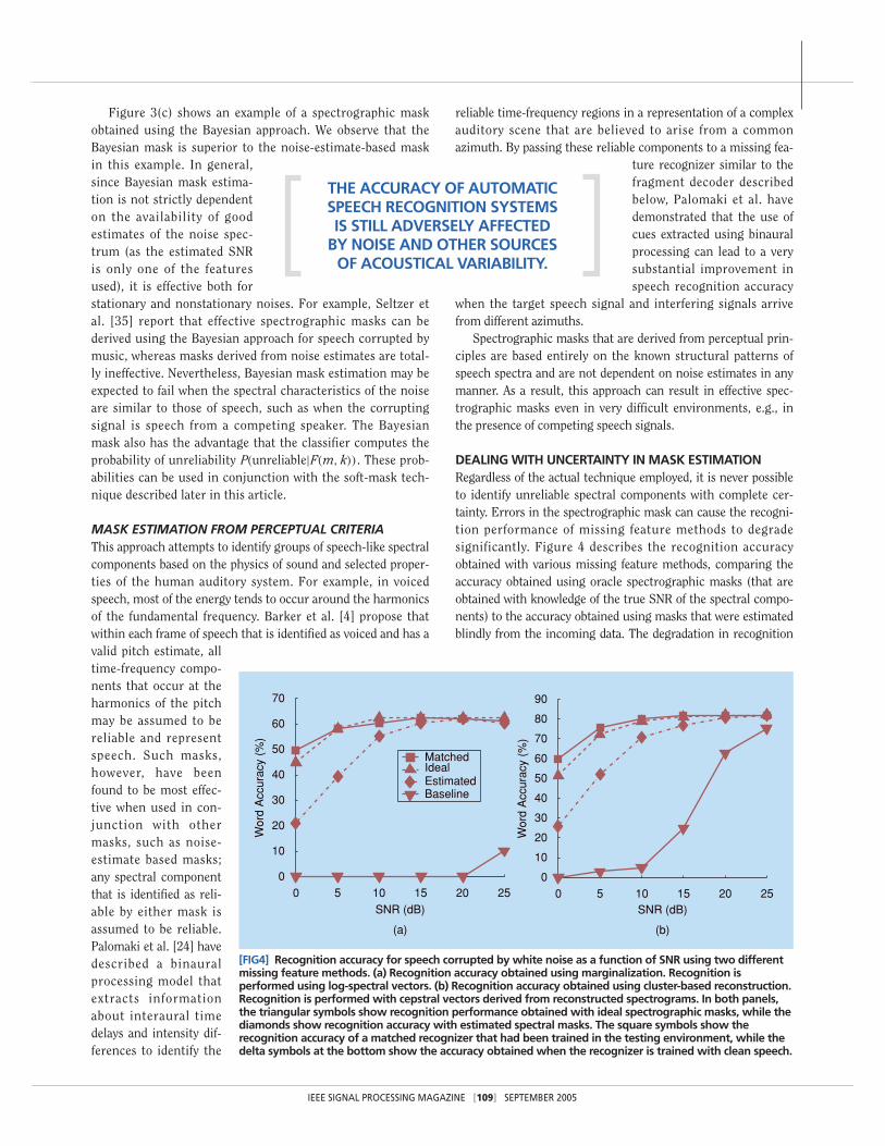
DEALING WITH UNCERTAINTY IN MASK ESTIMATIONRegardless of the actual technique employed, it is never possibleto identify unreliable spectral components with complete cer-tainty. Errors in the spectrographic mask can cause the recogni-tion performance of missing feature methods to degradesignificantly. Figure 4 describes the recognition accuracyobtained with various missing feature methods, comparing theaccuracy obtained using oracle spectrographic masks (that areobtained with knowledge of the true SNR of the spectral compo-nents) to the accuracy obtained using masks that were estimatedblindly from the incoming data. The degradation in recognition

[FIG4] Recognition accuracy for speech corrupted by white noise as a function of SNR using two differentmissing feature methods. (a) Recognition accuracy obtained using marginalization. Recognition isperformed using log-spectral vectors. (b) Recognition accuracy obtained using cluster-based reconstruction.Recognition is performed with cepstral vectors derived from reconstructed spectrograms. In both panels,the triangular symbols show recognition performance obtained with ideal spectrographic masks, while thediamonds show recognition accuracy with estimated spectral masks. The square symbols show therecognition accuracy of a matched recognizer that had been trained in the testing environment, while thedelta symbols at the bottom show the accuracy obtained when the recognizer is trained with clean speech.

0 5 10 15 20 250

10

20

30

40

50

60

70

80

90

SNR (dB)

Wor

d A

ccur

acy

(%)

0 5 10 15 20 250

10

20

30

40

50

60

70

SNR (dB)

(b)(a)

Wor

d A

ccur

acy

(%)

MatchedIdealEstimatedBaseline

THE ACCURACY OF AUTOMATICSPEECH RECOGNITION SYSTEMSIS STILL ADVERSELY AFFECTED

BY NOISE AND OTHER SOURCESOF ACOUSTICAL VARIABILITY.


accuracy due to errors in mask estimation is evident. We haveobserved that erroneous tagging of reliable components as beingunreliable degrades recognition accuracy more than taggingunreliable elements as reliable. More detailed analyzes of theeffects of mask estimation errors may be found in [28] and [35].

Two different remedies have been proposed to cope with theeffects of mask estimation errors. In the first approach, softmasks are estimated that represent the probability that a givenspectral component is reliable (as opposed to a binary mask thatunambiguously tags spectral components as reliable or unreli-able). In the second approach, the mask estimation is performedas a part of the speech recognition process itself, with the expec-tation that the detailed and precise statistical models for speechthat are used by the recognizer will also enable more accurateestimation of masks.

SOFT MASKSUnder the soft-decision framework, each spectral elementY(m, k) is assigned a probability γ = P(reliable|Y(m, k)) that itis reliable and dominated by speech rather than noise. The prob-ability of reliability is arrived at differently by different authors.The Bayesian mask estimation algorithms of Seltzer et al. [35]and Renevey et al. [31] can be used to obtain γ directly. Barkeret al. [6] employ an alternate approach, approximating γ as asigmoidal function of the estimated SNR of Y(m, k).

γ ≈ 11 + exp(−α(SNR(m, k) − β))

. (25)

The SNR itself is estimated from the estimated differences inlevel between speech and noise, using the proceduresdescribed previously. Typical values for α and β are 3.0 and 0.0,respectively.

Morris et al. [22] show that marginalization based on softmasks can be implemented with a relatively minor modificationto the bounded marginalization algorithm of (19) for HMM-based speech recognition systems that model state output densi-ties as mixtures of Gaussians with diagonal covariance matrices:

P(Y|s) =∑

k

∏

j

×

γ

e−(Y( j)−µs,k( j))2

2σs,k( j)

√2πσs,k( j)

+ (1 − γ )

Y(l)

∫ Y(l)

0

e−(x−µs,k(l))2

2σs,k( j)

√2πσs,k(l)

dx

.

(26)

Note that in (26) Y(l ) is the l th component of Y; (26) is equiva-lent to a model that assumes that spectral features are corruptedby a noise process that leaves them unchanged with a probabili-ty γ , or with a probability 1 − γ adds to them a random valuedrawn from a uniform probability distribution in the range(0, Y(l )). We also note that marginalization is the only missing

feature technique that can utilize soft masks effectively, sinceother techniques require unambiguous identification of unreli-able spectral components.

SIMULTANEOUS RECOGNITION AND MASK ESTIMATIONPossibly the most sophisticated missing feature technique is thespeech fragment decoder proposed by Barker et al. [3], [5]. Inthe speech fragment decoder the search mechanism used by thespeech recognizer is modified to derive the optimal spectro-graphic mask jointly with the optimal word sequence. In orderto do this, the Bayesian classification equation given in (5) ismodified to become

W, S = arg maxW,S

{P(W, S|Y)} (27)

where S represents any spectrographic mask and S representsthe optimal mask, and Y represents the entire spectral vectorsequence for the noisy speech. Letting X be the ideal spectralvector sequence for the clean speech underlying Y, this can beshown to be equal to

W, S = arg maxW,S

{P(W)

(∫P(X|W)

P(X|S, Y)

P(X)dX

)P(S|Y)

}

(28)

where P(S|Y) represents the probability of spectrographic maskS given the noisy spectral vector sequence Y, which is assumedto be independent of the word sequence W. In practical imple-mentations of HMM-based speech recognition systems, theoptimal state sequence is determined along with the best wordsequence. The corresponding modification to (27) used by thespeech fragment decoder is

W, S = arg maxW,S

maxs

P(S|Y)P(W)P(s|W)

×(

∏

m

∫P(X(t)|sm)

P(X(t)|S, Y)

P(X(m))dX(m)

)

. (29)

Here s represents a state sequence through the HMM for W,sm represents the mth state in the sequence, P(s|W) repre-sents the a priori probability of s and is obtained from thetransition probabilities of the HMM for W , X(m) representsthe mth vector in X, and P(X|s) represents the state outputdensity of s.

Let S(m) represent the spectrographic mask vector forY(m). Let U(m) represent the set of spectral components ofY(m) that are tagged as unreliable (or, alternately, as belongingto the background noise) by S(m). Let R(m) be the set of fre-quency bands that are identified as reliable. Let Y(m, j) andX(m, j) represent the j th component of Y(m) and X(m),


respectively. All state output densities are modeled as mixturesof Gaussians with diagonal covariance matrices, as given by (16).By further assuming that the conditional probabilitiesP(X(m, j)|S, Y ) are independent for the various values of j, andthat P(X(m, j)|S, Y ) is 0 for X(m, j) > Y(m, j) and propor-tional to P(X(m, j)) otherwise, and finally that the a prioriprobability of X(m, j) is a uniform density between 0 and xmax,the acoustic probability term within the parentheses on theright hand side of (29) is computed as

∫P(X(m)|sm)

P(X(m)|S, Y)

P(X(m))dX(m)

=∑

k

cst,k

∏

j∈R(m)

e−(Y(m, j)−µs,k( j))2

2σs,k( j)

∏

l∈U(m)

∫ Y(m,l)

0e

−(x−µs,k( j))2

2σs,k( j) xmax

Y(m, l)dx (30)

A complete implementation of (29) requires exhaustive evalu-ation of every possible spectrographic mask and is computa-tionally infeasible. Instead, the fragment decoder hypothesizesa large number of fragments or regions of the spectrogramwithin which all components are assumed to belong together.Fragments may be hypothesized based on various criteriaincluding SNR and acoustic cues such as harmonicity. Jointrecognition and search for the optimal spectrographic mask isperformed only over spectrographic masks that may beformed as combinations of these fragments. Barker et al.implement this procedure using a token-passing algorithmthat is described in [3].

The fragment-decoding approach has been shown by Barkeret al. to be more effective than simple bounded marginaliza-tion. It also has the advantage over other missing feature meth-ods that it can be easily extended to recognize multiple mixedsignals, such as those obtained from the combined speech ofmultiple simultaneous talkers. The only requirement is that theprecomputed fragments group spectral components from asingle speaker accurately.

ADDITIONAL PROCESSING OF SPECTRAL INPUTThe discussion thus far has assumed implicitly that recognitionis performed directly using the incoming spectral vectors as fea-tures. However, most speech recognizers preprocess incomingfeature vectors in various ways in order to improve recognitionaccuracy. For example, recognizers usually use cepstra derivedfrom log spectral vectors, rather than the log-spectral vectorsthemselves, because cepstral vectors are known to result insignificantly greater accuracy [13]. Recognition systems thatuse feature-vector imputation can work from cepstral vectorssince these can be derived from the complete spectral vectorsreconstructed by this approach. On the other hand, classifier-modification methods are generally ineffective for recognizersthat work from cepstral vectors, since they require informationthat characterizes the reliability of each component of the

incoming feature vectors, and such information is availableonly for spectral vectors.

Other common types of preprocessing of incoming featurevectors include augmentation using difference vectors andmean normalization of feature vectors. Again, while thesemanipulations do not pose problems for feature-vector recon-struction methods, classifier-modification methods must bemodified to accommodate them, and they in turn constrain thespecific missing feature methods that can be employed.

TEMPORAL-DIFFERENCE FEATURESIn most recognizers, the basic feature vector at any time isaugmented by difference and double-difference vectors.Difference vectors represent the trend, or velocity, of the fea-ture vectors and are usually obtained as the differencebetween adjacent feature vectors. The use of this informationpartially compensates for the commonly used but clearly inac-curate assumption that features extracted from successiveanalysis frames are statistically independent. The differencevector for frame m is obtained as

D(m) = Y(m + ξ) − Y(m − ξ) (31)

where D(m, k), the k th component of D(m) becomes unreli-able if either Y(m + ξ, k) or Y(m − ξ, k) is unreliable. Doubledifference vectors represent the acceleration of the spectralvectors and are computed as the difference between adjacentdifference vectors:

DD(m) = D(m + ζ ) − D(m − ζ ) (32)

DD(m, k) is unreliable if either D(m + ζ, k) or D(m − ζ, k) isunreliable. In the worst case, difference vectors may have asmuch as twice as many unreliable components on average asthe spectral vectors, while double difference vectors mayhave up to four times as many unreliable components. Inpractice, however, unreliable components tend to occur incontiguous patches, and the fraction of components in thedifference and double difference vectors that are unreliabletends not to be much greater than those of the spectral vec-tors themselves.

The upper and lower bounds on the values of unreliabledifference and double difference vector components must becomputed from the bounds on (or values of) the spectral compo-nents of which they are composed. For methods that use softmasks, the reliability probability of these terms must also bederived from the reliability probabilities of the spectral compo-nents from which they were computed.

MEAN NORMALIZATIONMean normalization [2] refers to the procedure by which themean feature vector of any sequence of feature vectors is sub-tracted from all vectors in the sequence, so that the resulting


sequence has zero mean. In symbolic terms, the mth normal-ized vector Y(m) of any sequence of feature vectorsY(1), Y(2), . . . , Y(M) is computed as

Y(m) = Y(m) − 1M

∑

mY(m). (33)

Mean normalization is commonly observed to result in largeimprovements in the recognition accuracy of automaticspeech recognitions systems.Unfortunately, mean normal-ization as described by (33)cannot be performed withclassifier-modifying missingfeature methods becausemany components of the fea-ture vectors used for recogni-tion are potentiallyunreliable. The mean valueof all vectors, as used in (33), would include the contributionsof these unreliable components and would be unreliable itself,and normalization by such a mean estimate results in degrada-tion of recognition performance [30]. Alternately, the meanvalue could be computed from only the reliable components ofthe spectrogram. Unfortunately, the reliable regions of spec-trograms contain chiefly high-energy spectral components,and mean estimates obtained from them tend to be biased,again resulting in degraded recognition performance.

A useful substitute for mean normalization has been pro-posed by Palomaki et al. [25]. Instead of subtracting the meanvalue of the spectral vector, every spectral component is nor-malized by a value that represents the upper percentile of thevalues for that component. Using this approach, Y(m, k), thenormalized value of Y(m, k), is computed as

Y(m, k) = Y(m, k) − 1D

∑

τ∈L

Y(τ, k) (34)

where L represents the set of frame indices of the D greatestY(m, k) values that are reliable. Palomaki et al. [25] observethat five is a good value for D, although lower values are alsoeffective. This approach has the advantage that the normaliza-tion term does not get biased by the presence of unreliable com-ponents in the spectrum. Thus, the normalization given by [34]can be effectively used with missing feature methods.

EXPERIMENTAL RESULTS AND DISCUSSIONIn this section we discuss and compare various aspects of miss-ing feature methods and their relative merits. Where possible,we present experimental evidence in support of our statements.We note that missing feature methods remains an active area ofresearch and that the techniques presented in this article havebeen developed by a number of people from a variety ofresearch groups. Since not all of these researchers have worked

on all aspects of the problem, it is not possible to identify a con-sistent set of results that have all been obtained on the samesystems and databases. Consequently, the experimental resultswe present in this article have been culled from a number ofpapers and sources. We have attempted to maintain a modicumof consistency where possible; most of the results describedhave been obtained from experiments conducted in theauthors’ laboratory at Carnegie Mellon University (CMU). TheCMU experiments were conducted using the ResourceManagement database [26], with the Sphinx-3 HMM-based

speech recognition system,with 2,000 tied state distribu-tions with Gaussian state out-put densities. We have mainlypresented results for speechcorrupted by white noise,although similar results havealso been obtained usingother noise types. Otherresults reported in this article

have been drawn from experiments conducted at the Universityof Sheffield and elsewhere, using the TI digits database. Wherewe report such results, the details of the experimental setupused for the experiments have been provided.

Speech is a highly redundant signal, with the evidence forany acoustic event being multiply represented in several fre-quency bands, often over several tens of milliseconds of time.Raj et al. [28] report that speech recognition performance doesnot degrade significantly when a randomly selected 80% of theelements are excised from a spectrogram and recognition is per-formed with only the remaining elements. Similar results havebeen reported by other researchers, e.g., Cooke et al. [9]. Themissing feature approach therefore promises to be highly effec-tive for noise-robust speech recognition. Traditionally, the beststrategy to recognize speech that has been corrupted by station-ary noise has been to train a matched recognizer with speechthat had been corrupted to the same level by the same kind ofnoise. Figure 4(a) and (b) compares the recognition accuracyobtained using matched recognizers on speech corrupted to var-ious SNRs by white noise, with the performance obtained withtwo different missing feature methods using ideal spectrograph-ic masks that had been derived with perfect knowledge of thetrue SNR of every spectrographic element, as well as using rec-ognizers that had been trained with clean speech. The recogni-tion accuracy performance obtained with the missing featuremethod is observed to be comparable to that obtained with amatched recognizer.

In practice, spectrographic masks must be estimated, andthe recognition accuracy obtained with estimated masks (alsoshown in Figure 4) is significantly worse than that obtainedusing ideal masks. Nevertheless, missing feature methods havethe advantage that the recognizer need not be retrained forevery noise type or level, and they also hold the promise thatthe performance could improve significantly with improvedmask estimation. More importantly, matched recognizers can-

MISSING FEATURE METHODS MODELTHE EFFECTS OF NOISE ON SPEECHAS THE CORRUPTION OF REGIONS

OF TIME-FREQUENCYREPRESENTATIONS OF THE

SPEECH SIGNAL.


not be trained for most practical situations, since the level andcharacteristics of the noise change even within the course ofan utterance. Instead, multistyle recognizers are trained thatattempt to strike an effective compromise across all theobserved noise types and levels. Experiments reported byBarker et al. [4] (Figure 5) show that missing feature methodscan outperform such recognizers even when the spectrograph-ic masks are estimated.

As noted earlier, highly nonstationary noises such as musicpose special problems for speech recognition systems.Conventional noise compensa-tion schemes are renderedineffective by such noises.However, missing featuremethods have been shown toresult in significant improve-ments in recognition accuracyeven on such noises (Figure 6).

Not all missing featuremethods are equivalent and useful in all situations, however,and different implementations have different characteristics.The SNR threshold that is used to determine which signal com-ponents are unreliable is typically higher for classifier-modifica-tion methods than for feature-imputation methods. For missingfeature methods with relatively low SNR thresholds for unrelia-bility, even spectral components tagged as reliable often have acertain degree of noise. For such methods, reducing the noiselevel in these components using a technique such a spectralsubtraction improves recognition accuracy [28]. For methodsfor which the SNR threshold for reliability is relatively high,spectral subtraction does not greatly improve accuracy.

Of the various missing feature methods, only marginaliza-tion and its derivative algorithms (soft-mask marginalizationand fragment decoding) purport to perform optimal classifica-

tion. Consequently the best recognition accuracy can be expectedfrom marginalization. Unfortunately, marginalization has thedisadvantage that recognition must be performed with spectralvector sequences directly. In general, however, recognition accu-racy obtained with cepstral vectors derived from spectral vectorsis much superior to that obtained with spectral vectors. Feature-imputation methods that reconstruct entire spectrogramsenable recognition with cepstral vectors derived from the recon-structed spectrograms. The benefits of going to the cepstraldomain often overcome the advantage gained by the optimal

classification performed withspectral vectors in marginal-ization, especially at highSNRs. This is demonstrated inFigure 7, which comparesrecognition performanceobtained with spectral andcepstral vectors using variousmissing feature methods.

Figure 7 and other results reported in the literature alsoshows that class-conditional imputation and covariance-basedreconstruction generally result in much poorer recognitionthan either marginalization or cluster-based reconstruction.However, these methods do have their uses. For example,Josifovski et al. [19] report that class-conditional imputation ishighly effective for reconstruction of complete spectrogramsfrom partial or unreliable ones. Raj et al. [28] show that whenspectrographic components are lost due to random deletions(e.g., due to loss during transmission), covariance-based recon-struction, which draws on information from adjacent vectors toreconstruct any missing component, is by far the best spectro-gram reconstruction method.

[FIG5] Comparison of recognition accuracy obtained usingmultistyle training and with soft-mask marginalization. Theexperiment was conducted on Test Set A of the Aurora corpus.Recognition was performed with spectral vectors.

−5 0 5 10 15 20 Clean0

20

40

60

80

100

SNR (dB)

Wor

d A

ccur

acy

(%)

Marginalization

Baseline

Multistyle

[FIG6] Recognition accuracy for speech corrupted by music. Thespectrographic mask was estimated using a Bayesian classifier,and unreliable components were reconstructed by cluster-basedreconstruction. Recognition was performed using cepstra derivedfrom reconstructed spectrograms. The lower curve shows therecognition accuracy obtained when no missing feature methodswere used. The RM database was used for this experiment, andthe recognizer was trained with clean speech.

0 5 10 15 20 250

10

20

30

40

50

60

70

80

SNR (dB)

Wor

d A

ccur

acy

(%)

Baseline

Cluster–Based Estimation

THE MOST DIFFICULT ASPECT OFMISSING FEATURE METHODS IS THE

ESTIMATION OF THE SPECTROGRAPHICMASKS THAT IDENTIFY UNRELIABLE

SPECTRAL COMPONENTS.

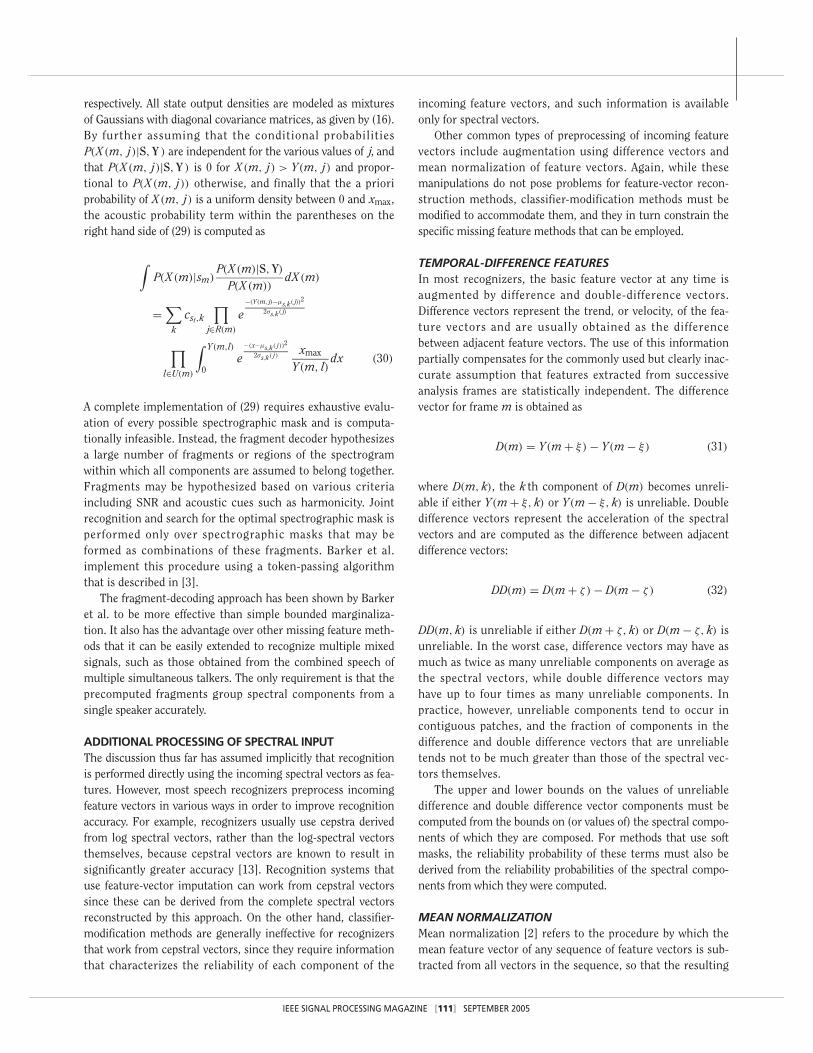
In considering the data in Figure 7 it should be noted thatthe relatively poor recognition results obtained using spectralcoefficients may be partially accounted for by the fact thatrecognition was performed using 20-dimensional log-spectralfeatures, with single-Gaussian HMM output distributions andno cepstral mean normalization or similar processing. Cepstralmean normalization was not employed in these experimentsbecause it cannot be meaningfully applied for the marginaliza-

tion method for the reasons discussed earlier. Cooke and hiscolleagues have suggested that the difference between therecognition accuracy obtained with spectral and cepstral vec-tors may be greatly reduced (although perhaps not eliminated)by using more detailed state output distributions for theHMMs. They have also noted that cepstral vectors are intrinsi-cally able to provide a greater degree of normalization for leveland spectral tilt than log-spectral features computed without

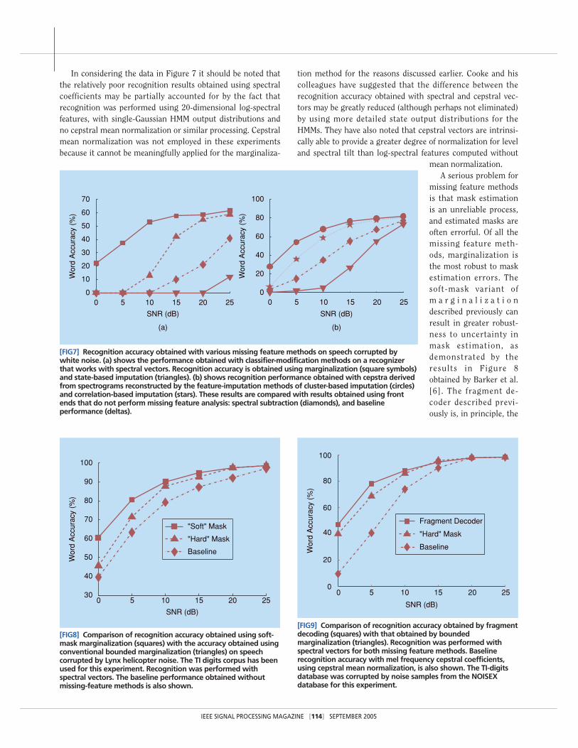
mean normalization.A serious problem for

missing feature methodsis that mask estimationis an unreliable process,and estimated masks areoften errorful. Of all themissing feature meth-ods, marginalization isthe most robust to maskestimation errors. Thesoft-mask variant ofm a r g i n a l i z a t i o ndescribed previously canresult in greater robust-ness to uncertainty inmask estimation, asdemonstrated by theresults in Figure 8obtained by Barker et al.[6]. The fragment de-coder described previ-ously is, in principle, the


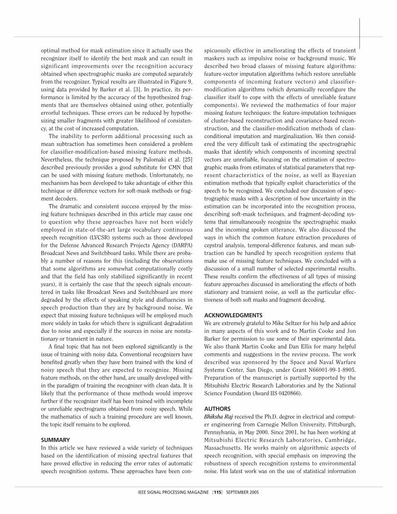
[FIG9] Comparison of recognition accuracy obtained by fragmentdecoding (squares) with that obtained by boundedmarginalization (triangles). Recognition was performed withspectral vectors for both missing feature methods. Baselinerecognition accuracy with mel frequency cepstral coefficients,using cepstral mean normalization, is also shown. The TI-digitsdatabase was corrupted by noise samples from the NOISEXdatabase for this experiment.

0 5 10 15 20 250

20

40

60

80

100

SNR (dB)

Wor

d A

ccur

acy

(%)

Fragment Decoder

"Hard" Mask

Baseline

[FIG8] Comparison of recognition accuracy obtained using soft-mask marginalization (squares) with the accuracy obtained usingconventional bounded marginalization (triangles) on speechcorrupted by Lynx helicopter noise. The TI digits corpus has beenused for this experiment. Recognition was performed withspectral vectors. The baseline performance obtained withoutmissing-feature methods is also shown.

0 5 10 15 20 2530

40

50

60

70

80

90

100

SNR (dB)

Wor

d A

ccur

acy

(%)

"Soft" Mask

"Hard" Mask

Baseline

[FIG7] Recognition accuracy obtained with various missing feature methods on speech corrupted bywhite noise. (a) shows the performance obtained with classifier-modification methods on a recognizerthat works with spectral vectors. Recognition accuracy is obtained using marginalization (square symbols)and state-based imputation (triangles). (b) shows recognition performance obtained with cepstra derivedfrom spectrograms reconstructed by the feature-imputation methods of cluster-based imputation (circles)and correlation-based imputation (stars). These results are compared with results obtained using frontends that do not perform missing feature analysis: spectral subtraction (diamonds), and baselineperformance (deltas).

0 5 10 15 20 250

10

20

30

40

50

60

70

SNR (dB)

Wor

d A

ccur

acy

(%)

(a)

0 5 10 15 20 250

20

40

60

80

100

SNR (dB)

Wor

d A

ccur

acy

(%)

(b)


optimal method for mask estimation since it actually uses therecognizer itself to identify the best mask and can result insignificant improvements over the recognition accuracyobtained when spectrographic masks are computed separatelyfrom the recognizer. Typical results are illustrated in Figure 9,using data provided by Barker et al. [3]. In practice, its per-formance is limited by the accuracy of the hypothesized frag-ments that are themselves obtained using other, potentiallyerrorful techniques. These errors can be reduced by hypothe-sizing smaller fragments with greater likelihood of consisten-cy, at the cost of increased computation.

The inability to perform additional processing such asmean subtraction has sometimes been considered a problemfor classifier-modification-based missing feature methods.Nevertheless, the technique proposed by Palomaki et al. [25]described previously provides a good substitute for CMN thatcan be used with missing feature methods. Unfortunately, nomechanism has been developed to take advantage of either thistechnique or difference vectors for soft-mask methods or frag-ment decoders.

The dramatic and consistent success enjoyed by the miss-ing feature techniques described in this article may cause oneto question why these approaches have not been widelyemployed in state-of-the-art large vocabulary continuousspeech recognition (LVCSR) systems such as those developedfor the Defense Advanced Research Projects Agency (DARPA)Broadcast News and Switchboard tasks. While there are proba-bly a number of reasons for this (including the observationsthat some algorithms are somewhat computationally costlyand that the field has only stabilized significantly in recentyears), it is certainly the case that the speech signals encoun-tered in tasks like Broadcast News and Switchboard are moredegraded by the effects of speaking style and disfluencies inspeech production than they are by background noise. Weexpect that missing feature techniques will be employed muchmore widely in tasks for which there is significant degradationdue to noise and especially if the sources in noise are nonsta-tionary or transient in nature.

A final topic that has not been explored significantly is theissue of training with noisy data. Conventional recognizers havebenefited greatly when they have been trained with the kind ofnoisy speech that they are expected to recognize. Missingfeature methods, on the other hand, are usually developed with-in the paradigm of training the recognizer with clean data. It islikely that the performance of these methods would improvefurther if the recognizer itself has been trained with incompleteor unreliable spectrograms obtained from noisy speech. Whilethe mathematics of such a training procedure are well known,the topic itself remains to be explored.

SUMMARYIn this article we have reviewed a wide variety of techniquesbased on the identification of missing spectral features thathave proved effective in reducing the error rates of automaticspeech recognition systems. These approaches have been con-

spicuously effective in ameliorating the effects of transientmaskers such as impulsive noise or background music. Wedescribed two broad classes of missing feature algorithms:feature-vector imputation algorithms (which restore unreliablecomponents of incoming feature vectors) and classifier-modification algorithms (which dynamically reconfigure theclassifier itself to cope with the effects of unreliable featurecomponents). We reviewed the mathematics of four major missing feature techniques: the feature-imputation techniquesof cluster-based reconstruction and covariance-based recon-struction, and the classifier-modification methods of class-conditional imputation and marginalization. We then consid-ered the very difficult task of estimating the spectrographicmasks that identify which components of incoming spectralvectors are unreliable, focusing on the estimation of spectro-graphic masks from estimates of statistical parameters that rep-resent characteristics of the noise, as well as Bayesianestimation methods that typically exploit characteristics of thespeech to be recognized. We concluded our discussion of spec-trographic masks with a description of how uncertainty in theestimation can be incorporated into the recognition process,describing soft-mask techniques, and fragment-decoding sys-tems that simultaneously recognize the spectrographic masksand the incoming spoken utterance. We also discussed theways in which the common feature extraction procedures ofcepstral analysis, temporal-difference features, and mean sub-traction can be handled by speech recognition systems thatmake use of missing feature techniques. We concluded with adiscussion of a small number of selected experimental results.These results confirm the effectiveness of all types of missingfeature approaches discussed in ameliorating the effects of bothstationary and transient noise, as well as the particular effec-tiveness of both soft masks and fragment decoding.

ACKNOWLEDGMENTSWe are extremely grateful to Mike Seltzer for his help and advicein many aspects of this work and to Martin Cooke and JonBarker for permission to use some of their experimental data.We also thank Martin Cooke and Dan Ellis for many helpfulcomments and suggestions in the review process. The workdescribed was sponsored by the Space and Naval WarfareSystems Center, San Diego, under Grant N66001-99-1-8905.Preparation of the manuscript is partially supported by theMitsubishi Electric Research Laboratories and by the NationalScience Foundation (Award IIS 0420866).

AUTHORSBhiksha Raj received the Ph.D. degree in electrical and comput-er engineering from Carnegie Mellon University, Pittsburgh,Pennsylvania, in May 2000. Since 2001, he has been working atMitsubishi Electric Research Laboratories, Cambridge,Massachusetts. He works mainly on algorithmic aspects ofspeech recognition, with special emphasis on improving therobustness of speech recognition systems to environmentalnoise. His latest work was on the use of statistical information

encoded by speech recognition systems for various signal pro-cessing tasks. He is a Member of the IEEE.

Richard M. Stern received the S.B. degree from theMassachusetts Institute of Technology (1970), the M.S. degreefrom the University of California, Berkeley (1972), and the Ph.D.from MIT (1977), all in electrical engineering. He has been onthe faculty of Carnegie Mellon University since 1977, where he iscurrently a professor in the Electrical and ComputerEngineering, Computer Science, and Biomedical EngineeringDepartments and the Language Technologies Institute. Much ofhis current research is in spoken language systems. He is partic-ularly concerned with the development of techniques to makeautomatic speech recognition more robust with respect tochanges in environmental and acoustical ambience. He has alsodeveloped sentence parsing and speaker adaptation algorithmsfor earlier CMU speech systems. In addition to his work inspeech recognition, he also maintains an active research pro-gram in psychoacoustics, where he is best known for theoreticalwork in binaural perception. He is a Member of the IEEE andthe Acoustical Society of America, and he was a recipient of theAllen Newell Award for Research Excellence in 1992.

REFERENCES[1] S. Ahmed and V. Tresp, “Some solutions to the missing feature problem invision,” in Advances in Neural Information Processing Systems 5. San Mateo, CA:Morgan Kauffman, 1993, pp. 393–400.

[2] B.S. Atal, “Effectiveness of linear prediction characteristics of the speech wavefor automatic speaker identification and verification,’’ J. Acoust. Soc. Amer., vol. 55, no. 6, pp. 1304–1312, 1974.

[3] J. Barker, M.P. Cooke, and D.P.W. Ellis, “Decoding speech in the presence ofother sources,’’ Speech Commun., vol. 45, no. 1, pp. 5–25, 2005.

[4] J. Barker, M. Cooke, and P. Green, “Robust ASR based on clean speech models:An evaluation of missing data techniques for connected digit recognition in noise,”in Proc. Eurospeech-2001. Aalborg, Denmark: 2001, pp. 213–216.

[5] J. Barker, M. Cooke, and D. Ellis, “Combining bottom-up and top-down con-straints for robust ASR: The multisource decoder,” in Proc. Workshop ConsistentReliable Acoustic Cues (CRAC), Sept. 2001.

[6] J. Barker, L. Josifovski, M. Cooke, and P. Green, “Soft decisions in missing datatechniques for robust automatic speech recognition,” in Proc. ICSLP 2000,Beijing, China, Sept. 2000, pp. 373–376.

[7] S. Boll, “Suppression of acoustic noise in speech using spectral subtraction,’’IEEE Trans. Acoust. Speech Signal Processing, vol. 27, no. 2, pp. 113–120, 1979.

[8] M.P. Cooke and D.P.W.E. Ellis, “The auditory organization of speech and othersources in listeners and computational models,’’ Speech Commun., vol. 35, no.3–4, pp. 141–177, 2001.

[9] M.P. Cooke, P.G. Green, and M.D. Crawford, “Handling missing data in speechrecognition,” in Proc. ICSLP-1994, Yokohama, Japan, 1994, pp. 1555–1558.

[10] M.P. Cooke, A. Morris, and P.D. Green, “Missing data techniques for robustspeech recognition,” in Proc. IEEE Conf. Acoustics, Speech, Signal Processing,Munich, Germany, 1997, pp. 863–866.

[11] M. Cooke, P. Green, L. Josifovski, and A. Vizinho, “Robust ASR with unreliabledata and minimal assumptions,’’ in Proc., Robust’99, Tampere, Finland, 1999, pp.195–198.

[12] M. Cooke, P. Green, L. Josifovski, and A. Vizinho, “Robust Automatic SpeechRecognition with missing and unreliable acoustic data,’’ Speech Commun., vol. 34,no. 3, pp. 267–285, 2000.

[13] S.B. Davis and P. Mermelstein, “Comparison of parametric representations formonosyllabic word recognition in continuously spoken sentences,’’ IEEE Trans.Acoust., Speech, Signal Processing, vol. 28, no. 4, pp. 357–366, 1980.

[14] A.P. Dempster, N.M. Laird, and D.B. Rubin, “Maximum likelihood from incom-plete data via the EM algorithm,” J. Royal Stat. Soc., vol. 39, no. 1, pp. 1–38, 1977.

[15] M. El-Maliki and A. Drygajlo, “Missing features detection and handling forrobust speaker verification,’’ in Proc. Eurospeech 1999, Budapest, Hungary, pp.975–978.

[16] B.J. Frey, L. Deng, A. Acero, and T. Kristjansson, “ALGONQUIN: IteratingLaPlace’s method to remove multiple types of acoustic distortion for robust speechrecognition,’’ in Proc. Eurospeech 2001, Aalborg, Denmark, 2001, pp. 901–904.

[17] H. Fletcher, Speech and Hearing in Communication. New York: VanNostrand, 1953.

[18] H.G. Hirsch and C. Ehrlicher, “Noise estimation techniques for robust speechrecognition,’’ in Proc. IEEE Conf. Acoustics, Speech Signal Processing, Detroit,Michigan, 1995, pp. 153–156.

[19] L. Josifovski, M. Cooke, P. Green, and A. Vizihno, “State based imputation ofmissing data for robust speech recognition and speech enhancement,’’ in Proc.Eurospeech, Budapest, Hungary, 1999, pp. 2837–2840.

[20] R.P. Lippmann and B.A. Carlson, “Using missing feature theory to activelyselect features for robust speech recognition with interruptions, filtering andnoise,’’ in Proc. Eurospeech, Rhodes, Greece, 1997, pp. KN37–KN40.

[21] B.C.J. Moore and B.R. Glasberg, “Suggested formulae for calculating auditory-filter bandwidths and excitation patterns,’’ J. Acoust. Soc. Amer., vol. 74, no. 3, pp. 750–753, 1983.

[22] A.C. Morris, J. Barker, and H. Bourlard, “From missing data to maybe usefuldata: Soft data modelling for noise robust ASR,’’ in Proc. WISP 2001, Stratford-upon-Avon, U.K., 2001.

[23] P.J. Moreno, “Speech recognition in noisy environments,” Ph.D. dissertation,ECE Dept., Carnegie Mellon Univ., Pittsburgh, PA, May 1996.

[24] K.J. Palomaki, G.J. Brown, and D.L. Wang, “A binaural processor for missingdata speech recognition in the presence of noise and small-room reverberation,’’Speech Commun., vol. 43, no. 4, pp. 361–378, Sept. 2004.

[25] K.J. Palomaki, G.J. Brown, and J. Barker, “Techniques for handling convolu-tional distortion with ‘missing data’ automatic speech recognition,’’ SpeechCommun., vol. 43, no. 1–2, pp. 123–142, 2004.

[26] P. Price, W.M. Fisher, J. Bernstein, and D.S. Pallet, “The DARPA 1000 wordresource management database for continuous speech recognition,’’ in Proc. IEEEConf. Acoustics, Speech Signal Processing, New York, 1988, pp. 651–654.

[27] L.R. Rabiner and B.-H. Juang, Fundamentals of Speech Recognition.Englewood Cliffs, NJ: Prentice-Hall, 1993.

[28] B. Raj, “Reconstruction of incomplete spectrograms for robust speech recogni-tion,” Ph.D. dissertation, ECE Dept., Carnegie Mellon Univ., Pittsburgh, PA, Apr. 2000.

[29] B. Raj, V. Parikh, and R.M. Stern, “The effects of background music on speechrecognition accuracy,’’ in Proc. IEEE Conf. Acoustics, Speech Signal Processing,Munich, Germany, 1997, pp. 851–854.

[30] B. Raj, M.L. Seltzer, and R.M. Stern, “Reconstruction of missing features forrobust speech recognition,’’ Speech Commun. J., vol. 43, no. 4, pp. 275–296, 2004.

[31] P. Renevey and A. Drygajlo, “Missing feature theory and probabilistic estima-tion of clean speech components for robust speech recognition,’’ in Proc.EUROSPEECH, Budapest, Hungary, 1999, pp. 2627–2630.

[32] P. Renevey and A. Drygajlo, “Detection of reliable features for speech recogni-tion in noisy conditions using a statistical criterion,’’ in Proc. WorkshopConsistent Reliable Acoustic Cues (CRAC), Aalborg, Denmark, 2001.

[33] P. Renevey, “Speech in noisy conditions using missing feature approach,” Ph.D.dissertation, Swiss Federal Institute of Technology, Lousanne, Switzerland, 2001.

[34] D.B. Rubin, Multiple Imputation for Nonresponse in Surveys. New York:Wiley, 1987.

[35] M.L. Seltzer, B. Raj, and R.M. Stern, “A bayesian framework for spectrographicmask estimation for missing feature speech recognition,’’ Speech Commun. J., vol.43, no. 4, pp. 379–393, 2004.

[36] A. Vizinho, P. Green, M. Cooke, and L. Josifovski, “Missing data theory, spec-tral subtraction and signal-to-noise estimation for robust ASR: An integratedstudy,’’ in Proc. Eurospeech, Budapest, Hungary, 1999, pp. 2407–2410.


[SP]

missing-feature approaches in speech recognition drobust/papers/rajstern_spmag.pdf · mathematics...

Documents