(un)expected monetary policy shocks and term … · increase of policy rate =⇒ different samples,...

(Un)expected Monetary Policy Shocks and

Term premia: A Bayesian Estimated

Macro-Finance Model

Martin Kliem (Bundesbank)Alexander Meyer-Gohde (Uni Hamburg)

26. January 2018

Disclaimer

The views expressed in this presentation are those of the authors and donot reflect the opinions of the Deutsche Bundesbank.

Introduction Model Solution & Estimation Results Conclusion 1 / 23

Introduction

Model

Solution & Estimation

Results

Conclusion

Research Question

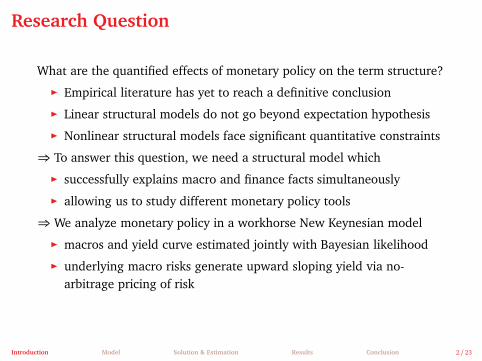
What are the quantified effects of monetary policy on the term structure?

◮ Empirical literature has yet to reach a definitive conclusion

◮ Linear structural models do not go beyond expectation hypothesis

◮ Nonlinear structural models face significant quantitative constraints

⇒ To answer this question, we need a structural model which

◮ successfully explains macro and finance facts simultaneously

◮ allowing us to study different monetary policy tools

⇒ We analyze monetary policy in a workhorse New Keynesian model

◮ macros and yield curve estimated jointly with Bayesian likelihood

◮ underlying macro risks generate upward sloping yield via no-arbitrage pricing of risk


This paper estimates a structural model

. . .with time-variation in risk premia

1985 1990 1995 2000 2005

0

1

2

3

4

5

6

7

Nom

inal 10−

year

term

pre

miu

m in %

Model

Corresponding estimates in the literature

Figure : Model implied 10-year nominal term premium (black line) and range ofcorresponding estimates in the literature (gray area).


Main findings I

◮ Predicts upward sloping nominal and real yield curves◮ Real risk premia play important role→ 70% real risk, 30% inflation risk

◮ Historical smoothed time series for bonds and risk premia→ comparable to empirical estimates


Some empirical evidence

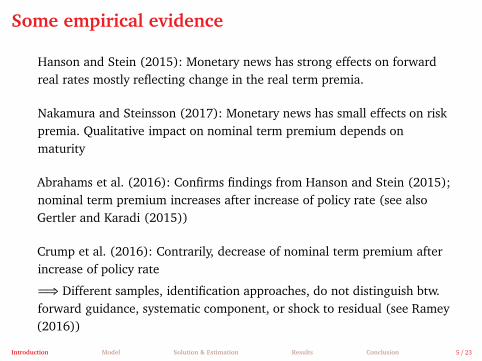
Hanson and Stein (2015): Monetary news has strong effects on forwardreal rates mostly reflecting change in the real term premia.

Nakamura and Steinsson (2017): Monetary news has small effects on riskpremia. Qualitative impact on nominal term premium depends onmaturity

Abrahams et al. (2016): Confirms findings from Hanson and Stein (2015);nominal term premium increases after increase of policy rate (see alsoGertler and Karadi (2015))

Crump et al. (2016): Contrarily, decrease of nominal term premium afterincrease of policy rate

=⇒ Different samples, identification approaches, do not distinguish btw.forward guidance, systematic component, or shock to residual (see Ramey(2016))


Main findings II

◮ A standard MP shock has small effects on term premium (see Naka-mura and Steinsson (2017))

◮ A shock to the systematic component of MP has larger and longlasting effects on term premium (see Hanson and Stein (2015))

◮ Unconditional forward guidance increases real and inflation risk oflong-term bonds

→ Nominal term premium increases (see Akkaya et al. (2015)) whichdampens the expansionary effect


Introduction

Model


Results

Conclusion

Model overview

◮ general equilibrium macro-finance model (e.g. Rudebusch andSwanson (2012); Andreasen et al. (2017))◮ closed-economy New-Keynesian DSGE◮ nominal and real frictions◮ external habit formation◮ long-run nominal and real risk◮ price stickiness (Calvo)◮ monetary policy characterized by Taylor-rule

◮ consumption-based asset pricing (arbitrage-free, frictionless)

⇒ we use recursive preferences (Epstein-Zin-Weil) to disentangleintertemporal elasticity of substitution and risk aversion


Monetary Policy

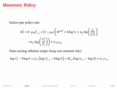
Taylor-type policy rule:

4rft =4 ·ρRr

f

t−1 + (1−ρR)

�

4rreal + 4 logπt +ηy log

�

yt

z+t y

�

+ηπ log

�

π4t

π∗t

��

+σmεm,t

Time-varying inflation target (long–run nominal risk):

logπ∗t− 4 log π= ρπ�

logπ∗t−1 − 4 log π�

+ 4ζπ (logπt−1 − log π) +σπεπ,t


Bond pricing

Nominal zero-coupon bond prices (p(0)t = 1 and p(0)t = 1):

Risky: p(n)t = Et

�

Mt,t+1p(n−1)t+1

�

, Risk neutral: p(n)t =�

Rft

�−1Et

�

p(n−1)t+1

�

The continuously compounded return of n-period bond is defined as:

r(n)t = −

1

nlog p

(n)t

Term premium: difference between the risky and risk-neutral returns

TP(n) =1

n

�

log p(n)t − log p

(n)t

�

= −1

nEt

n−1∑

j=0

e−rt,t+j+1 covt+j

�

Mt+j+1,p(n−j−1)t+j+1

�


Introduction

Model


Results

Conclusion

Higher-order solution technique (see Meyer-Gohde

(2016))

◮ We adjust point and slope for risk out to second moments

◮ capture both constant and time-varying risk premium

◮ risk-sensitive linear approximation around the ergodic mean

⇒ non-certainty-equivalent approximation, but linear in states

⇒ This allows us to use the standard set of tools for estimation andanalysis of linear models, without limiting the approximation to thecertainty-equivalent approximation around the deterministic steady state.


Linear Non-Certainty Equivalent Approximation

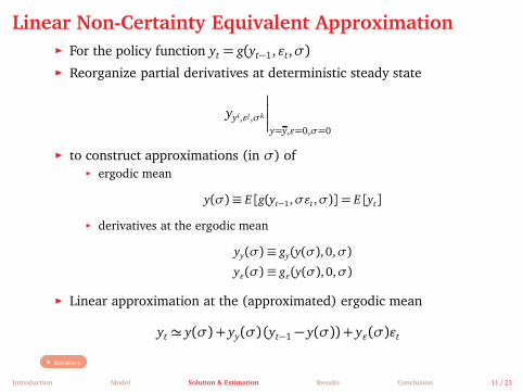
◮ For the policy function yt = g(yt−1,ǫt,σ)

◮ Reorganize partial derivatives at deterministic steady state

yyi,ǫj,σk

�

�

�

�

y=y,ǫ=0,σ=0

◮ to construct approximations (in σ) of◮ ergodic mean

y(σ) ≡ E [g(yt−1,σǫt,σ)] = E [yt]

◮ derivatives at the ergodic mean

yy(σ) ≡ gy(y(σ), 0,σ)

yǫ(σ) ≡ gǫ(y(σ), 0,σ)

◮ Linear approximation at the (approximated) ergodic mean

yt ≃ y(σ) + yy(σ) (yt−1 − y(σ)) + yǫ(σ)ǫt

Accuracy


Estimation

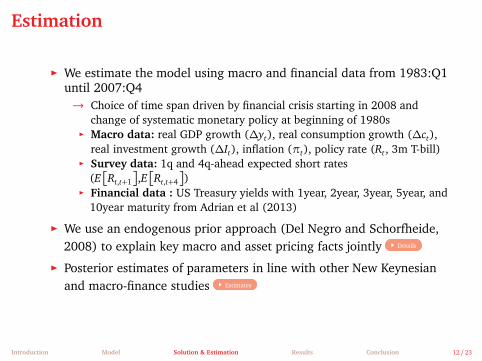
◮ We estimate the model using macro and financial data from 1983:Q1until 2007:Q4→ Choice of time span driven by financial crisis starting in 2008 and

change of systematic monetary policy at beginning of 1980s◮ Macro data: real GDP growth (∆yt), real consumption growth (∆ct),

real investment growth (∆It), inflation (πt), policy rate (Rt, 3m T-bill)◮ Survey data: 1q and 4q-ahead expected short rates

(E�

Rt,t+1

�

,E�

Rt,t+4

�

)◮ Financial data : US Treasury yields with 1year, 2year, 3year, 5year, and

10year maturity from Adrian et al (2013)

◮ We use an endogenous prior approach (Del Negro and Schorfheide,2008) to explain key macro and asset pricing facts jointly Details

◮ Posterior estimates of parameters in line with other New Keynesianand macro-finance studies Estimates


Introduction

Model


Results

Conclusion

Predicted nominal yield curve

0 10 20 30 40

Maturity (Quarter)

5

5.5

6

6.5

7

7.5

An

nu

aliz

ed

Yie

lds in

%

Median

Data

Figure : Nominal Yield Curve

Why is the nominal yield curve upward sloping?


Predicted term structure of interest rates

0 10 20 30 40

Maturity (Quarter)

2.5

3

3.5

4

4.5

5

5.5

6

6.5

7

Annualiz

ed Y

ield

s in %

Det. Steady State

Median

(a) Real Yield Curve

0 10 20 30 40

Maturity (Quarter)

0

50

100

150

200

Annualiz

ed P

rem

ia in B

asis

Poin

ts

Det. Steady State

Median

(b) Nominal Term Premium

0 10 20 30 40

Maturity (Quarter)

0

20

40

60

80

100

120

140

160

Annualiz

ed P

rem

ia in B

asis

Poin

ts

Det. Steady State

Median

(c) Real Term Premium

0 10 20 30 40

Maturity (Quarter)

0

10

20

30

40

50

60

70

Annualiz

ed P

rem

ia in B

asis

Poin

ts

Det. Steady State

Median

(d) Inflation risk premium

Why is the real yield curve upward sloping?


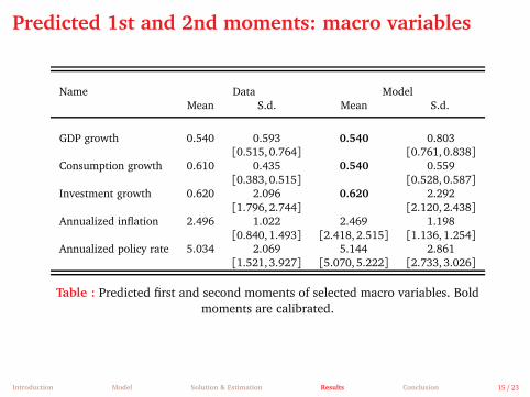
Predicted 1st and 2nd moments: macro variables

Name Data ModelMean S.d. Mean S.d.

GDP growth 0.540 0.593 0.540 0.803[0.515, 0.764] [0.761, 0.838]

Consumption growth 0.610 0.435 0.540 0.559[0.383, 0.515] [0.528, 0.587]

Investment growth 0.620 2.096 0.620 2.292[1.796, 2.744] [2.120, 2.438]

Annualized inflation 2.496 1.022 2.469 1.198[0.840, 1.493] [2.418, 2.515] [1.136, 1.254]

Annualized policy rate 5.034 2.069 5.144 2.861[1.521, 3.927] [5.070, 5.222] [2.733, 3.026]

Table : Predicted first and second moments of selected macro variables. Boldmoments are calibrated.


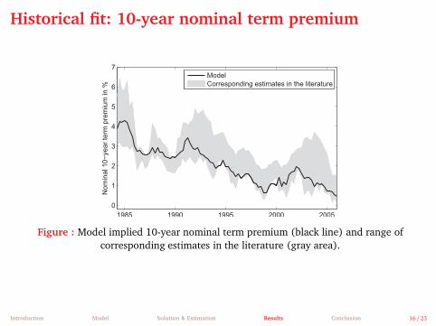
Historical fit: 10-year nominal term premium

1985 1990 1995 2000 2005

0

1

2

3

4

5

6

7

Nom

inal 10−

year

term

pre

miu

m in %

Model

Corresponding estimates in the literature

Figure : Model implied 10-year nominal term premium (black line) and range ofcorresponding estimates in the literature (gray area).


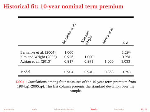
Historical fit: 10-year nominal term premium

Bern

anke

etal

.

Kim

and

Wrig

ht

Adria

net

al.

S.d.

Bernanke et al. (2004) 1.000 1.294Kim and Wright (2005) 0.976 1.000 0.981Adrian et al. (2013) 0.817 0.891 1.000 1.033

Model 0.904 0.940 0.868 0.943

Table : Correlations among four measures of the 10-year term premium from1984:q1-2005:q4. The last column presents the standard deviation over the

sample.


Historical fit: 10-year real rate

1985 1990 1995 2000 2005

Year

0

1

2

3

4

5

6

7

8

in p

erc

ent %

10-year real rate (model)

10-year TIPS

Chernov and Mueller (JFE,2012)

Figure : Model implied 10-year real rates (red solid), 10-year TIPS of Gürkaynaket al. (2010) (black dashed), and 10-year real rate of Chernov and Mueller

(2012)(blue dash-dotted).


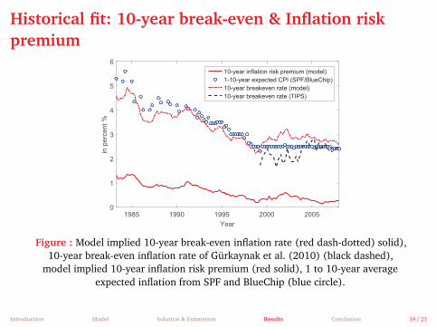
Historical fit: 10-year break-even & Inflation risk

premium

1985 1990 1995 2000 2005

Year

0

1

2

3

4

5

6

in p

erc

ent %

10-year inflation risk premium (model)

1-10-year expected CPI (SPF/BlueChip)

10-year breakeven rate (model)

10-year breakeven rate (TIPS)

Figure : Model implied 10-year break-even inflation rate (red dash-dotted) solid),10-year break-even inflation rate of Gürkaynak et al. (2010) (black dashed),

model implied 10-year inflation risk premium (red solid), 1 to 10-year averageexpected inflation from SPF and BlueChip (blue circle).


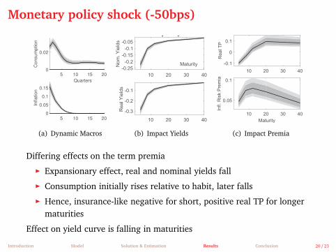
Monetary policy shock (-50bps)

5 10 15 20

Consum

ption

0

0.02

5 10 15 20

Inflation

0

0.05

0.1

0.15

Quarters

(a) Dynamic Macros

10 20 30 40

-0.25

-0.2

-0.15

-0.1

-0.05

No

m.

Yie

lds

Monetary Policy Shock

10 20 30 40

-0.3

-0.2

-0.1

Maturity

Re

al Y

ield

s

(b) Impact Yields

10 20 30 40

-0.1

0

0.1

Re

al T

P

10 20 30 40

Maturity

0.05

0.1

Infl.

Ris

k P

rem

ia

(c) Impact Premia

Differing effects on the term premia

◮ Expansionary effect, real and nominal yields fall

◮ Consumption initially rises relative to habit, later falls

◮ Hence, insurance-like negative for short, positive real TP for longermaturities

Effect on yield curve is falling in maturities


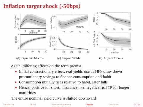
Inflation target shock (-50bps)

5 10 15 20

Co

nsu

mp

tio

n

5 10 15 20

Infla

tio

n

5 10 15 200

0.1

0.2

5 10 15 20

-2

-1

0Quarters

(d) Dynamic Macros

10 20 30 40

10 20 30 40R

eal Y

ield

s

10 20 30 40

-1

-0.5

Inflation Target Shock

10 20 30 40

0

0.2

0.4

0.6

Maturity

Nom

. Y

ield

s

(e) Impact Yields

10 20 30 40

Re

al T

P

10 20 30 40

Infl.

Ris

k P

rem

ia

10 20 30 40

-10

-5

0

5

10 20 30 40

Maturity

-8

-6

-4

-2

(f) Impact Premia

Again, differing effects on the term premia◮ Initial contractionary effect, real yields rise as HHs draw down

precautionary savings to finance consumption and habit◮ Consumption initially rises relative to habit, later falls◮ Hence, positive for short, insurance-like negative real TP for longer

maturities

The entire nominal yield curve is shifted downward


Forward guidance (-50bps in 4 quarters)

Quarters

0

0.05

0.1

5 10 15 200

0.5

1

Co

nsu

mp

tio

nIn

fla

tio

n

5 10 15 20

(g) Dynamic Macros

No

m.

Yie

lds

Re

al Y

ield

s

4 10 20 30 40

-0.12-0.1

-0.08-0.06-0.04-0.02

4 10 20 30 40

-0.6

-0.4

-0.2

Maturity

(h) Impact Yields

Real T

PIn

fl. R

isk P

rem

ia Maturity4 10 20 30 40

-0.5

0

0.5

4 10 20 30 40

0.4

0.6

(i) Impact Premia

Large expansionary effect with a significant rise in inflation◮ Inflationary effects reduce response of nominal yield curve

◮ directly over the expectations hypothesis and◮ both inflation risk and real TP rise for all but short maturities→ total nominal TP nearly 1 bp for all but shortest maturities

◮ Only the very short end of the yield curve moves

Rise in real TP dampens expansionary effect Details of Implementation


Introduction

Model


Results

Conclusion

Conclusion

◮ estimated DSGE model with time-varying risk premia

◮ in line with empirical facts about the term structure

◮ structural model well-suited to investigate effects of monetary policyon risk premia

◮ shocks to the Taylor-rule have small effects on risk premia

◮ shocks to systematic component of monetary policy much more long-lasting and therefore larger effects on term premia

◮ forward guidance increases risk premia [→] especially for longermaturities


References I

ABRAHAMS, M., T. ADRIAN, R. K. CRUMP, E. MOENCH, AND R. YU (2016):“Decomposing real and nominal yield curves,” Journal of MonetaryEconomics, 84, 182–200.

ADRIAN, T., R. K. CRUMP, AND E. MOENCH (2013): “Pricing the termstructure with linear regressions,” Journal of Financial Economics, 110,110–138.

AKKAYA, Y., R. GÜRKAYNAK, B. KISACIKOGLU, AND J. WRIGHT (2015):“Forward guidance and asset prices,” IMES Discussion Paper Series, E-6.

ANDREASEN, M. M., J. FERNÁNDEZ-VILLAVERDE, AND J. F. RUBIO-RAMÍREZ

(2017): “The Pruned State-Space System for Non-Linear DSGE Models:Theory and Empirical Applications,” Review of Economic Studies,forthcoming.

BACKUS, D. K., A. W. GREGORY, AND S. E. ZIN (1989): “Risk premiums inthe term structure : Evidence from artificial economies,” Journal ofMonetary Economics, 24, 371–399.

A-1 /A-14

References II

BERNANKE, B. S., V. R. REINHART, AND B. P. SACK (2004): “Monetary PolicyAlternatives at the Zero Bound: An Empirical Assessment,” BrookingsPapers on Economic Activity, 35, 1–100.

CHERNOV, M. AND P. MUELLER (2012): “The term structure of inflationexpectations,” Journal of Financial Economics, 106, 367–394.

CRUMP, R. K., S. EUSEPI, AND E. MOENCH (2016): “The term structure ofexpectations and bond yields,” Staff report, FRB of NY.

DEL NEGRO, M., M. GIANNONI, AND C. PATTERSON (2015): “The forwardguidance puzzle,” Staff Reports 574, Federal Reserve Bank of New York.

DEL NEGRO, M. AND F. SCHORFHEIDE (2008): “Forming priors for DSGEmodels (and how it affects the assessment of nominal rigidities),”Journal of Monetary Economics, 55, 1191–1208.

DEN HAAN, W. J. (1995): “The term structure of interest rates in real andmonetary economies,” Journal of Economic Dynamics and Control, 19,909–940.

A-2 /A-14

References III

GERTLER, M. AND P. KARADI (2015): “Monetary policy surprises, creditcosts, and economic activity,” American Economic Journal:Macroeconomics, 7, 44–76.

GÜRKAYNAK, R. S., B. SACK, AND J. H. WRIGHT (2010): “The TIPS YieldCurve and Inflation Compensation,” American Economic Journal:Macroeconomics, 2, 70–92.

HANSON, S. G. AND J. C. STEIN (2015): “Monetary policy and long-termreal rates,” Journal of Financial Economics, 115, 429–448.

HÖRDAHL, P., O. TRISTANI, AND D. VESTIN (2008): “The Yield Curve andMacroeconomic Dynamics,” Economic Journal, 118, 1937–1970.

KIM, D. H. AND J. H. WRIGHT (2005): “An arbitrage-free three-factor termstructure model and the recent behavior of long-term yields anddistant-horizon forward rates,” Finance and Economics DiscussionSeries 2005-33, Board of Governors of the Federal Reserve System(U.S.).

A-3 /A-14

References IV

LASÉEN, S. AND L. E. SVENSSON (2011): “Anticipated Alternative PolicyRate Paths in Policy Simulations,” International Journal of CentralBanking.

MEYER-GOHDE, A. (2016): “Risk-Sensitive Linear Approximations,”mimeo, Hamburg University.

NAKAMURA, E. AND J. STEINSSON (2017): “High frequency identificationof monetary non-neutrality: The information effect,” Quarterly Journalof Ecnomics, forthcoming.

PIAZZESI, M. AND M. SCHNEIDER (2007): “Equilibrium Yield Curves,” inNBER Macroeconomics Annual 2006, Volume 21, National Bureau ofEconomic Research, Inc, NBER Chapters, 389–472.

RAMEY, V. A. (2016): “Macroeconomic Shocks and Their Propagation,” inHandbook of Macroeconomics, ed. by J. B. Taylor and H. Uhlig, Elsevier,vol. 2, chap. 2, 71–162.

A-4 /A-14

References V

RUDEBUSCH, G. D. AND E. T. SWANSON (2012): “The Bond Premium in aDSGE Model with Long-Run Real and Nominal Risks,” AmericanEconomic Journal: Macroeconomics, 4, 105–43.

WACHTER, J. A. (2006): “A consumption-based model of the term structureof interest rates,” Journal of Financial Economics, 79, 365–399.

A-5 /A-14

Accuracy of Approximation

0 2 4 6 8 10 12 14 16 18 20−5

−4

−3

−2

−1

0

1Impulse Responses of 3y Term Premium to a Technology Shock

Quarter since Shock Realization

Deviations from Steady−State in bps

Risk−Sensitive

First−Order Accurate

Third−Order Accurate

◮ Risk-sensitive not as accurate as full third-order perturbation

◮ But does captures the third-order dynamics remarkably well . . .

◮ . . . even though the solution is linear in states and shocks

Return

A-6 /A-14

Endogenous prior (Del Negro and Schorfheide, 2008)

posterior:

p (θ |X,S,F)∝ p (θ |F,S)× p (X|θ)

∝ p (θ)× p (F|Fm (θ))× p (S|θ)× p (X|θ)

◮ p (θ) initial set of prior

◮ p (F|Fm (θ)) quasi-likelihood related to first moments we have apriori information about

◮ p (S|θ) likelihood related to second moments we have a prioriinformation about, here variance of ∆y,∆c,∆I,π,R (see Christiano,Trabandt and Walentin, 2011)

◮ p (X|θ) likelihood related to data

A-7 /A-14

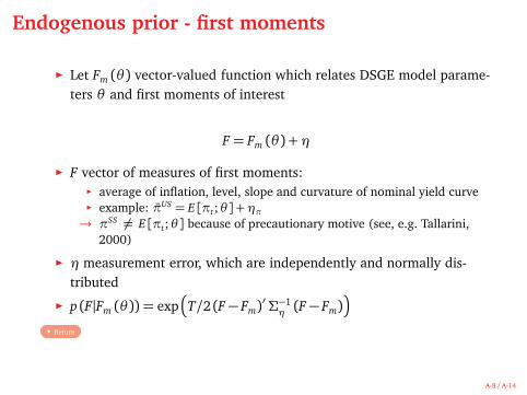
Endogenous prior - first moments

◮ Let Fm (θ) vector-valued function which relates DSGE model parame-ters θ and first moments of interest

F = Fm (θ) +η

◮ F vector of measures of first moments:◮ average of inflation, level, slope and curvature of nominal yield curve◮ example: πUS = E [πt;θ ] +ηπ→ πSS 6= E [πt;θ ] because of precautionary motive (see, e.g. Tallarini,

2000)

◮ η measurement error, which are independently and normally dis-tributed

◮ p (F|Fm (θ)) = exp�

T/2 (F − Fm)′Σ−1η(F − Fm)�

Return

A-8 /A-14

Selected parameter estimates

Name Mode Mean 5% 95%

Relative risk aversion 89.860 91.427 75.581 108.489Calvo parameter 0.853 0.855 0.843 0.866Habit formation 0.685 0.679 0.614 0.741Intertemporal elas. substitution 0.089 0.089 0.077 0.101Steady state inflation 1.038 1.034 0.981 1.091Interest rate smoothing coefficient 0.754 0.752 0.718 0.786Interest rate inflation coefficient 3.124 3.164 2.839 3.491Interest rate output coefficient 0.156 0.159 0.114 0.204

Table : Posterior stats. Post. means and parameter dist.: MCMC, 2 chains, 100,000draws each, 50% of the draws used for burn-in, and draw acceptance rates ≈ 1/3.

Return

A-9 /A-14

Calibration

Description Symbol Value

Technology trend in percent z+ 0.54/100Investment trend in percent Ψ 0.08/100Capital share α 1/3Depreciation rate δ 0.025Price markup θp/(θp − 1) 1.2Price indexation ξp 0Discount factor β 0.99Frisch elasticity of labor supply FE 0.5Labor supply l 1/3Ratio of government consumption to output g/y 0.19

Table : Parameter calibration.

A-10 /A-14

Model fit

1985 1990 1995 2000 20050

0.05

0.1

corr=0.998

1985 1990 1995 2000 20050

0.05

0.1

corr=1.000

1985 1990 1995 2000 20050

0.05

0.1

corr=1.000

1985 1990 1995 2000 20050

0.05

0.1

corr=0.999

1985 1990 1995 2000 20050

0.05

0.1

0.15

corr=0.994

1985 1990 1995 2000 20050

0.05

0.1

0.15

corr=0.979

1985 1990 1995 2000 20050

0.05

0.1

0.15

corr=0.939Model

Data

R4,t R8,t R12,t R20,t

R40,t Et [Rt,t+1] Et [Rt,t+4]

Figure : Observed and model implied nominal returns of treasury bills and returnsof expected short rates.

A-11 /A-14

Why is the nominal yield curve upward sloping?

◮ Backus et al. (1989), den Haan (1995)

◮ in a recession short rates are low, so long-term bonds should havehigher price

→ bonds should carry an insurance-like premium

◮ But: in a recession induced by supply shocks→ inflation goes up

→ real value of the bond decreases

→ dominant role of supply shocks explain slope (Piazzesi and Schnei-der, 2007)

TP(n) = −1

nEt

n−1∑

j=0

e−rt,t+j+1 covt+j

�

Mt+j+1,p(n−j−1)t+j+1

�

Return

A-12 /A-14

Why is the real yield curve upward sloping?

◮ Following Wachter (2006) and Hördahl et al. (2008)

◮ habit formation induces positive autocorrelation in consumptiongrowth

◮ households will seek to maintain their habit in the face of a slow-down in consumption

→ drawing down precautionary savings→ long-term bond price falls

→ negative correlation between stochastic discount factor and bondprices

TP($,n) = −1

nEt

n−1∑

j=0

e−rt,t+j+1 covt+j

�

M$t+j+1,p($,n−j−1)

t+j+1

�

Return

A-13 /A-14

Modelling forward guidanceSequence of anticipated policy shocks to model forward guidance◮ Laséen and Svensson (2011), Del Negro et al. (2015)

Resulting in the following change to the standard interest rate rule:

Rt = R(Rt−1,πt,Yt) +

K∑

k=0

εt,t+k

where εt,t+k is a shock known to agents at time t, but realized at time t+ k.

As our equilibrium system is linear in states,◮ Finding the anticipated shocks to condition the interest rate path◮ simply requires solving a square linear system of dimension k

Po

licy R

ate

5 10 15 20

-0.4

-0.2

0

Return

A-14 /A-14

(un)expected monetary policy shocks and term … · increase of policy rate =⇒ different samples,...

Documents