applied tddft - i: a chemist’s...

Joaquim Jornet-Somoza

nano-biospectroscopygroup

1 Nano-Bio Spectroscopy Group and ETSF Scientific Development Center, Departamento de Física de Materiales, Centro de Física de Materiales CSIC-UPV/EHU and DIPC,

University of the Basque Country UPV/EHU, Avenida Tolosa 72, 20018 Donostia/San Sebastián, Spain

Applied TDDFT - I: a Chemist’s Perspective

1

[email protected]

mailto:[email protected]?subject=

Outline

• Chemist’s Interests ? • What’s is chemistry? • GS chemistry = Thermochemistry • ES chemistry = photochemistry

• Theoretical Methods for Excited State in Chemistry

• Optical Properties from TDDFT:• Linear Response Theory • LRTDDFT : CASIDA Equations, TDA • Real-Time Propagation TDDFT

• Failures of TDDFT• Charge-Transfer excitations • PES topology

2

Outline


• Theoretical Methods for Excited State in Chemistry



3

Chemist’s Interests 4

Chemistry is a branch of physical science that studies the composition, structure, properties and change of matter. Chemistry includes topics such as the properties of individual atoms, how atoms form chemical bonds to create chemical compounds, the interactions of substances through intermolecular forces that give matter its general properties, and the interactions between substances through chemical reactions to form different substances.

Chemistry is sometimes called the central science because it bridges other natural sciences, including physics, geology and biology.

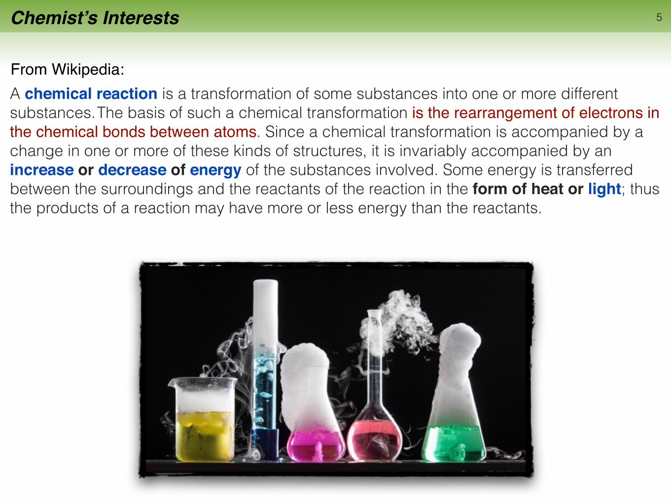
From Wikipedia:

https://en.wikipedia.org/wiki/Chemical_bond

https://en.wikipedia.org/wiki/Natural_science


A chemical reaction is a transformation of some substances into one or more different substances. The basis of such a chemical transformation is the rearrangement of electrons in the chemical bonds between atoms. Since a chemical transformation is accompanied by a change in one or more of these kinds of structures, it is invariably accompanied by an increase or decrease of energy of the substances involved. Some energy is transferred between the surroundings and the reactants of the reaction in the form of heat or light; thus the products of a reaction may have more or less energy than the reactants.

From Wikipedia:

https://en.wikipedia.org/wiki/Chemical_reaction

https://en.wikipedia.org/wiki/Endothermic_reaction

https://en.wikipedia.org/wiki/Exothermic_reaction

https://en.wikipedia.org/wiki/Energy

https://en.wikipedia.org/wiki/Photochemistry


ReactantsProduct

Reaction Coordinate

Ener

gy

Chemical Reaction

Computational interest: Study the energetics and mechanism of the reaction

TS

Chemical Reaction: transformation from reactants to products


A theoretical/computational approach will therefore need: • theoretical model for matter in the energy range [0 to few hundred of eV] • description of the interaction with the environment (condensed phase) • description of chemical reactions (structural changes)

From Wikipedia:A chemical reaction is a transformation of some substances into one or more different substances. The basis of such a chemical transformation is the rearrangement of electrons in the chemical bonds between atoms. Since a chemical transformation is accompanied by a change in one or more of these kinds of structures, it is invariably accompanied by an increase or decrease of energy of the substances involved. Some energy is transferred between the surroundings and the reactants of the reaction in the form of heat or light; thus the products of a reaction may have more or less energy than the reactants.


… which translates into: • electronic structure theory and ways to solve the corresponding equations • approximate solutions for the description of the interaction with the environment.

• solution of the equations of motion for atoms and electrons + statistical mechanics (from the microcanonical to the canonical ensemble)



… and in practice: • HF, CI, MPn, CAS, ..., DFT and corresponding theories for excited states • periodic boundary conditions, PBC, for homogeneous systems and hybrid schemes, for

inhomogeneous systems: QM/MM, coarse grained, hydrodynamics, ... • time dependent theories for adiabatic and non adiabatic dynamics of atoms and

electrons: mixed-quantum classical molecular dynamics



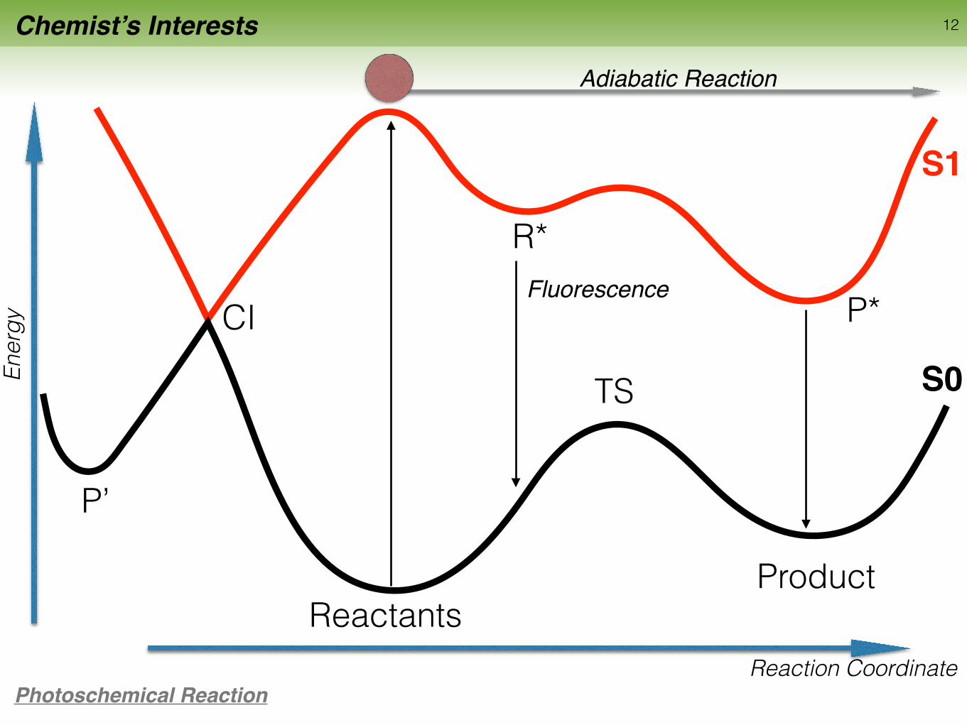
Photochemistry is the branch of chemistry concerned with the chemical effects of light. Generally, this term is used to describe a chemical reaction caused by absorption of ultraviolet (wavelength from 100 to 400 nm), visible light (400 – 750 nm) or infrared radiation (750 – 2500 nm). Photochemical reactions are mainly of only specialized value in organic and inorganic chemistry. In nature, photochemistry is of immense importance as it is the basis of photosynthesis, vision, and the formation of vitamin D with sunlight. Photochemical reactions proceed differently than thermal reactions. Photochemical paths access high energy intermediates that cannot be generated thermally, thereby overcoming large activation barriers in a short period of time, and allowing reactions otherwise inaccessible by thermal processes.

From Wikipedia:

https://en.wikipedia.org/wiki/Chemistry

https://en.wikipedia.org/wiki/Ultraviolet

https://en.wikipedia.org/wiki/Wavelength

https://en.wikipedia.org/wiki/Nanometre

https://en.wikipedia.org/wiki/Visible_light

https://en.wikipedia.org/wiki/Infrared

https://en.wikipedia.org/wiki/Organic_chemistry

https://en.wikipedia.org/wiki/Inorganic_chemistry

https://en.wikipedia.org/wiki/Vitamin_D


ReactantsProduct

TS

Reaction Coordinate

Ener

gy

Photoschemical Reaction

P’

Adiabatic Reaction

R*

P*CI

S0

S1


ReactantsProduct

TS

Reaction Coordinate

Ener

gy


P’

Adiabatic Reaction

R*

P*CI

S0

S1

Fluorescence


ReactantsProduct

TS

Reaction Coordinate

Ener

gy


P’

Adiabatic Reaction

R*

P*CI

S0

S1

Phosphorescence


ReactantsProduct

TS

Reaction Coordinate

Ener

gy


P’

Non-Adiabatic Reaction

R*

P*CI

S0

S1

Non-radiative Decay


ReactantsProduct

TS

Reaction Coordinate

Ener

gy

P’

R*

P*CI

S0

S1

15

How do we can describe the energy landscape from first-principles ?

Outline 16


• Theoretical Methods for Excited State Chemistry



Excited States in Quantum Chemistry

Wavefunction-based methods

17

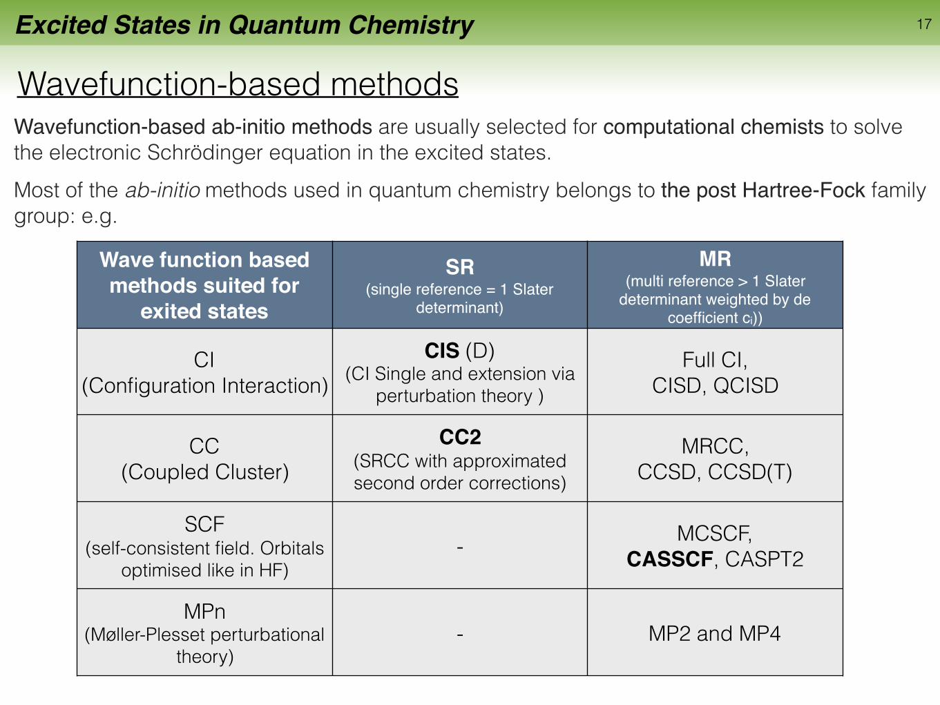
Wavefunction-based ab-initio methods are usually selected for computational chemists to solve the electronic Schrödinger equation in the excited states.Most of the ab-initio methods used in quantum chemistry belongs to the post Hartree-Fock family group: e.g.

Wave function based methods suited for

exited states

SR (single reference = 1 Slater

determinant)

MR (multi reference > 1 Slater

determinant weighted by de coefficient ci))

CI (Configuration Interaction)

CIS (D) (CI Single and extension via

perturbation theory )

Full CI, CISD, QCISD

CC (Coupled Cluster)

CC2(SRCC with approximated second order corrections)

MRCC, CCSD, CCSD(T)

SCF (self-consistent field. Orbitals

optimised like in HF)- MCSCF,

CASSCF, CASPT2

MPn (Møller-Plesset perturbational

theory)- MP2 and MP4

Excited States in Quantum Chemistry 18

All post Hartree-Fock methods are based on the expansion of the many-electron wavefunction in a linear combination of “excited” Slater determinants:

| i = c0|�0i+X

ia

cai |�ai i+

X

i<ja<b

cabij |�abij i+

X

i<j<ka<b<c

cabcijk |�abcijki+ · · ·

The different quantum chemical methods for the electronic structure (ground and excited states) differ in the way this (infinite) sum is approximated.

In comparison of the HF method, these expansion corrects a hight percentage the so called electronic correlation (i.e. the difference between the exact energy and the HF energy)

In all cases, the results can always be improved by increasing the number of allowed excitation to expand the ansatz: singles(S), doubles (D), triples (T) …

Most of the computational cost rely on the evaluation of the large number of four-centre electron repulsion integrals

Kia,bj =

Zd3r

Zd3r0�⇤

ia(r)fH�jb(r0); �ia(r) = '⇤

i (r)'a(r)

19

Among the single reference (SR) methods:

Practical Issues

CIS: is practically no longer used in the calculation of excitation energies in molecules.The error in the correlation energy is usually very large and gives qualitatively wrong results. STILL good to gain insights into CT states energies. Largely replaced by TDDFT.

CC2: is a quite recent development and therefore not widely available. Accurate and fast, is the best alternative to TDDFT. Good energies also for CT states.

Multi reference (MR) ab initio methods are still computationally too expensive for large systems (they are limited to few tenths of atoms) and for mixed-quantum classical dynamics. However, there are many interesting new developments (MR- CISD, G-MCQDPT2, RI-CC2, EOM-CC2).


20

Practical Issues

TDDFT for excitation energies of large systems:

is formally exact and improvements of the xc-functionals are still possible.

is computationally more efficient and scales better than ab-initio wavefunction-based methods.

can be used for large systems (up to thousand atoms).

can be easily combined with MD (mixed quantum classical MD)


BUT is not a black box !

Alternative to wavefunction-based methods:

Outline 21





Optical properties from TDDFT

Brief Review of the time-dependent KS equations

22

The effect of the phase-factor is simply to introduce an additive constant to the total action

A[⇢] =

Z t1

t0

h (t)|i @@t

� H(t)| (t)idt+ �1 � �0 = A[⇢] + const.

The role played by the 2nd Hohenberg-Kohn theorem in the derivation of the time-dependent DFT equation is now “played” by a variational principle involving the action:

Where the wavefunction is determined by the initial conditions up to a time-dependent phase factor:

(t) = [⇢, 0] · e�i�(t)

A[ ] =

Z t1

t0

h (t)|i @@t

� H(t)| (t)idt

Then the true density, which determine the action, is the one that make the action stationary,Runge-Gross Theorem - II

Corrected action density functional (causality and symmetry paradox): R. van Leeuwen PRL 80, 1280 (1998)

0 =�A[⇢]

�⇢(r, t)=

Z t1

t0

h � (t0)

�⇢(r, t)|i @

@t0� H(t0)| (t0)idt0 + c.c.


The density functional action can be re-written in terms of a universal density functional which does not depend on the external potential,

A[⇢] = B[⇢]�Z

dr

Zt1

t0

vext

(r;R, t)⇢(r, t)dt

In analogy with the ground state density function theory, we may assume an independent particle system whose orbitals have the property:

⇢(r, t) =X

i

fi|'i(r, t)|2

interacting density non-interacting KS orbital

23

Assuming that the effective potential exists (v-representability problem), the universal functional can be expressed as

exchange-correlation action functional

B[⇢] =X

i

fi

Zt1

t0

dth'i

(t)|i @@t

� 1

2r2

i

|'i

(t)i

� 1

2

Zt1

t0

dt

Z Zdr1r2

⇢(r1, t)⇢(r2, t)

|r1 � r2|�A

xc

[⇢]

Optical properties from TDDFT 24

Minimizing the action functional (variational principle),

A[⇢] = B[⇢]�Z

dr

Zt1

t0

vext

(r;R, t)⇢(r, t)dt

we obtain the time-dependent KS equations:h� 1

2r2 + veff (r, t)

i'i(r, t) = i

@

@t'i(r, t)

where,

Hartree Exchange Correlation potentialExternal

veff

(r, t) = vext

+

Z⇢(r, t)

|r � r0|dr0 + v

xc

(r, t)

Where the unknown is now the time-dependent XC potential, defined as

vxc

(r, t) =�A

xc

[⇢]

�⇢(r, t)

In analogy to the traditional time-independent Kohn-Sham scheme, all exchange and correlation effects in TDDFT are collected in to the �A

xc

[⇢]/�⇢(r, t)

In the formal derivation of the TDDFT equations no approximations are made, and therefore the theory is in principle exact.


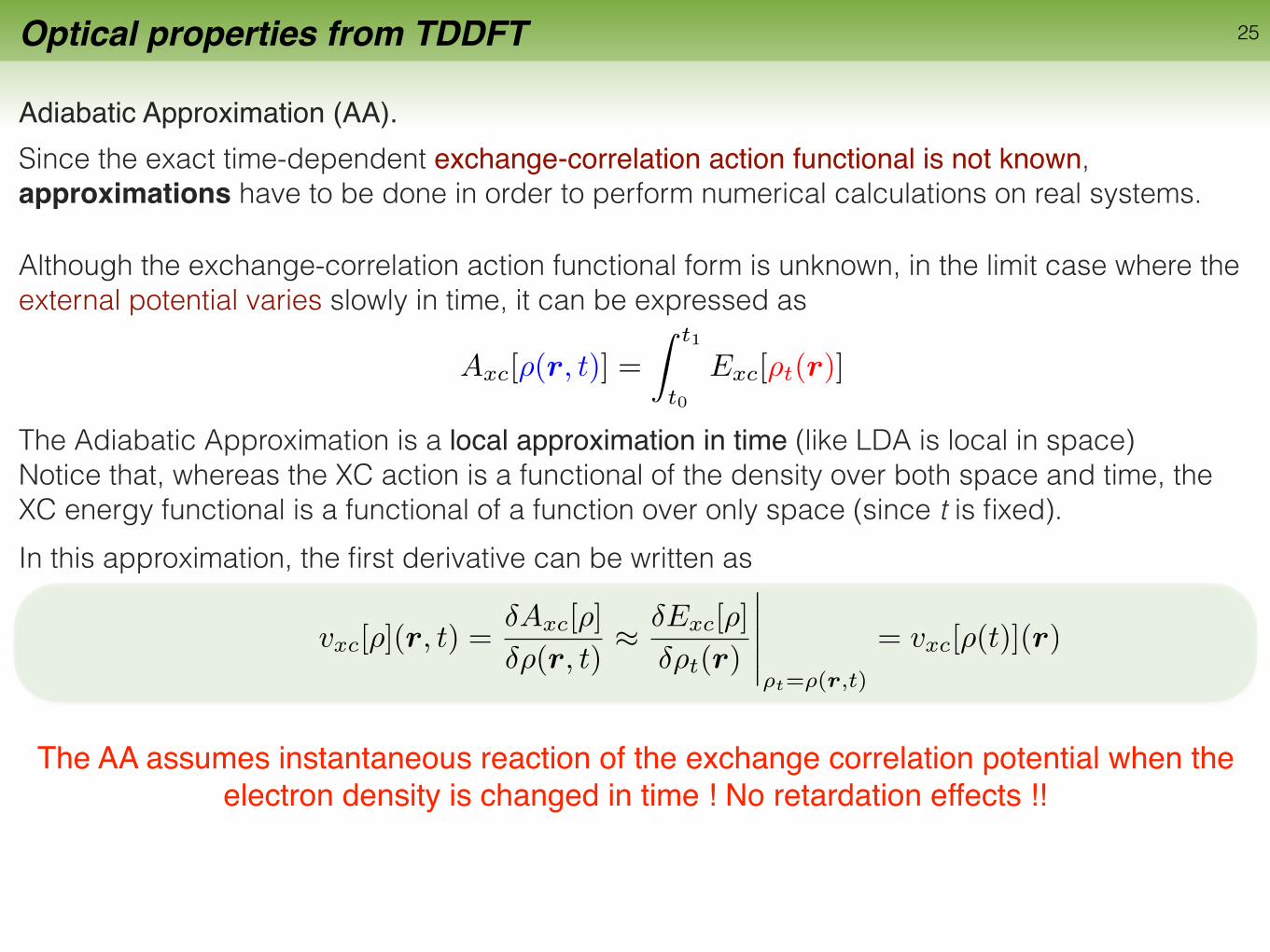
Adiabatic Approximation (AA).

25

Since the exact time-dependent exchange-correlation action functional is not known, approximations have to be done in order to perform numerical calculations on real systems.

The AA assumes instantaneous reaction of the exchange correlation potential when the electron density is changed in time ! No retardation effects !!

Although the exchange-correlation action functional form is unknown, in the limit case where the external potential varies slowly in time, it can be expressed as

The Adiabatic Approximation is a local approximation in time (like LDA is local in space) Notice that, whereas the XC action is a functional of the density over both space and time, the XC energy functional is a functional of a function over only space (since t is fixed).

Axc

[⇢(r, t)] =

Zt1

t0

Exc

[⇢t

(r)]

In this approximation, the first derivative can be written as

vxc

[⇢](r, t) =�A

xc

[⇢]

�⇢(r, t)⇡ �E

xc

[⇢]

�⇢t

(r)

��⇢t=⇢(r,t)

= vxc

[⇢(t)](r)


Practical Issues about the Adiabatic Approximation (AA).

Within this approximation, we can use all xc functionals, vxc(r), derived for the time-independent DFT also for the time-dependent functionals vxc(r)|t and fxc(r)|t (including hybrid functionals)

Due to this approximation works well beyond its domain of rigorous justification, and to its relative simplicity, the AA approximation has become the work house of the TDDFT.

Some known failures of the Adiabatic Approximation

We neglect all retardation or memory effects. This can easily be seen in AA xc kernel:

- Frequency-dependence in xc-kernel is essential for the description of double excited states. - Rabi oscillation are not well reproduced.

f

xc

(rt, r0t0) ⇠= �(t� t

0)�

2E

xc

[rho]

�⇢

t

(r)⇢t

0(r0)


Linear Response Theory

27

⇢(r, t) = ⇢0(r, t) + �⇢(r, t)

The main quantity in LRT is the density-density response function

The basis of linear response formulation is the change of the density of a system under the influence of an external time dependent perturbation, �v

ext

�(r, r0, t� t0) =�⇢(r, t)

�vext

(r0, t0)

��v0

Notice that the response have to be zero at any time before t’.

which relates the first order density response with to the applied perturbation

�⇢(r, t) =

Zt

t0

dt0Z

dr0�(r, r0, t� t0)�vext

(r0, t0)

where the total external potentials is given by the sum of the stationary initial state potential, usually GS, and the external perturbation potential

vext

(r, t) = v0(r) + �vext

(r, t)


For our purpose, it is convenient to introduce the matrix formalism of the response density, in second quantisation. Assuming a complete basis set of time-independent orthonormal orbitals, {ψi}, the linear response of the density matrix is defined by

�Pij = h� 0(t)|a†j ai| 0(t)i+ h 0(t)|a†j ai|� 0(t)i

Where are the corresponding creation and annihilation operators.a†j , ai

The response of the density matrix can be also expressed in terms of the generalised susceptibility 𝛘 ,

�Pij

(t) =X

kl

Z +1

�1�ij,kl

(t� t0)�vextkl

dt0

After doing some algebra, we can write it as,

�Pij

(t1) =X

kl

Z +1

�1

(� i⇥(t1 � t)

X

I 6=0

hh 0|a†

j

ai

| I

ih 0|a†k

al

| I

ie�i(EI�E0�i⌘)(t1�t)

�h 0|a†k

al

| I

ih I

|a†j

ai

| 0ie�i(E0�EI�i⌘)(t1�t)i)

�vextkl

(t)dt


Then, taking the Fourier Transform gives the sum-over-states representation of the generalised susceptibility (Lehmann representation)

accounts for excitations and relaxation contributions

�ij,kl(!) =X

I 6=0

(h 0|a†j ai| Iih 0|a†kal| Ii

! � ⌦I + i⌘�

h 0|a†kal| Iih I |a†j ai| 0i! + ⌦I + i⌘

)

(notice that all reference to the spin components has been avoided for simplicity)

A special case is that of a single particle systems with the Schrödinger equation

h i = ✏i i

for such systems, and keeping in the second quantisation notation, the generalised susceptibility reads,

�ij,kl(!) = �i,k�j,lfj � fi

! � (✏i � ✏j)

being fi the occupation of the orbital i.


Exercise: Derive the expression of the dynamics polarisability, knowing

The sum-over-states expressions can also be derived for particular response properties. Of particular interest in molecular spectroscopy is the computation of the dynamics polarisability, α(ω), which is the response function that relates an electric external potential to the change of the dipole.

µ⌫(t) = µ⌫(t0) +

Z +1

�1↵⌫�(t� t0)E�(t0)dt0

µ⌫ = qr⌫

�vext�

(t) = r�

E(t)

dipole moment operator

external electric field

↵⌫�(t� t0) = �i⇥(t� t0)h 0|[µ⌫(t� t0), r�]| 0idynamic polarizability


Exercise: Derive the expression of the dynamics polarisability, knowing

µ⌫ = qr⌫ �vext�

(t) = r�

E(t) ↵⌫�(t� t0) = �i⇥(t� t0)h 0|[µ⌫(t� t0), r�]| 0i

dipole operator external electric field dynamic polarisability

We consider a complete set of eigenfunctions {Ψn}, n = 0, 1, 2 …, of the unperturbed system, and the completeness relation 1 =

X1

n=0| nih n|

↵µ�(!) = � lim⌘!0+

1X

n=1

(h 0|r⌫ | nih n|r�| 0i

! � ⌦n + i⌘� h 0|r�| nih n|r⌫ | 0i

! + ⌦n + i⌘

)

take into account the negative charge of the electron density

↵µ�(!) =1X

n=1

(2⌦nh 0|r⌫ | nih n|r�| 0i

⌦2n � !2

)

h 0|r⌫ | nih n|r�| 0i = h 0|r�| nih n|r⌫ | 0i

Making use of the fact that

and arranging terms, we obtain


↵µ�(!) =1X

n=1

(2⌦nh 0|r⌫ | nih n|r�| 0i

⌦2n � !2

)The general expression of the dynamic polarisability is then written as

This result is interesting because it shows that excitation energies

fn =2⌦n

3

3X

µ=1

|h n|rµ| 0i|2

and the spectroscopic oscillator strength, ⌦n = En � E0

are the poles and residues of the mean polarisability

↵(!) =1

3tr↵(!) =

1X

n=1

fn⌦2

n � !2

And then, the optical spectrum is defined by the photoabsorption cross-section:

�(!) =4⇡!

3c=m[↵(!)]


The response of an interacting system with an external electric field can be obtained if we know the excitation energies and oscillator strength.

↵(!) =1

3tr↵(!) =

1X

n=1

fn⌦2

n � !2

Summary:

However, considering the difficulty of calculating accurate transition energies and oscillator strength (which requires knowing the continuum states as well as bound states), it is usually much easier to compute the polarisability directly, using its matrix representation

↵⌫�(!) =�µ⌫(!)

E�(!)= �

X

ij,kl

r⌫ji�ij,kl(!)r�kl

density-density response function

(r⌘ab = h a|r⌘| bi)

Now the problems becomes into the computation of the response function for an interacting system. Here is when TDDFT takes its important role.

The poles of the response function of the physical system will correspond to the pole of the dynamic polarisability.

Outline 34



• Optical Properties from TDDFT:• Linear Response Theory • LRTDDFT : CASIDA Equations, TDA• Real-Time Propagation TDDFT



Linear Response in Khon-Sham Realm (LR-TDDFT)

35

LR-TDDFT aims to obtain the response function of a physical system from the fact that is it possible to obtain the real time-dependent electron density if we know an effective potential of a non-interacting electron system. The response function of the physical system of interacting electrons can be computed from the Dyson-like equation

�(!) = �s(!) + �s(!) ? fHxc(!) ? �(!)

where the space dependence has been omitted for simplicity, the indicates integrals over space, and the Hartree and Exchange correlation functional is the Fourier transform of:

fHxc(r1t, r2t0) =

�(t� t0)

|r1 � r2|+

�vxc[⇢](r, t)

�⇢(r0, t0)

And the non-interacting response function in a base of Kohn-Sham orbitals reads as

�s(r, r0,!) = lim

⌘!0+

X

k,j

(fk � fj)��k�j

'(0)⇤k (r)'(0)

j (r)'(0)⇤j (r0)'(0)

k (r0)

! � (✏j � ✏k) + i⌘


Now, integrating both sides of Dyson-like equation agains the external perturbation potential, we obtain

The exact density-response has poles at the true excitation energies. However, these are not identical to the KS excitation energies. The true excitation energies are therefore those frequencies where the eigenvalue of the integral operator (left h.s.) vanishes.

h1� �s(!) ? fHxc(!)

i? �⇢(!) = �s(!) ? �vext(!)

Different solutions have been proposed to find the poles of the true response function:

· Casida’s Equation: matrix formulation of the TDDFT linear response (M. E. Casida 1995, 1996) · Tamm-Dancoff approximation in TDDFT: neglects backwards transitions (S. Hiarta & M. Head-Gordon 1999) · Single-Pole Approximation: expand all quantities around one particular KS energy difference (Petersilka 1999) · Sternheimer method: apply time-dependent perturbation theory, often applied to extended systems (ref?)


Casida´s Equations

37

The first matrix formulation of the TDDFT linear response was derived by M.E. Casida. He showed that the excitation energies of a physical system can be obtained by solving the system of equations

where

Notice that the frequency dependence of the matrices A and B has been dropped assuming the Adiabatic Approximation of the Hartree-Exchange Correlation kernel.

✓A BB⇤ A⇤

◆✓XY

◆= ⌦

✓�I 00 I

◆✓XY

◆

Aia,jb = �ia�jb(✏a � ✏i) + 2

Zd3r

Zd3r0�⇤

ia(r)fHxc�jb(r0)

Bia,jb = 2

Zd3r

Zd3r0�⇤

ia(r)fHxc�bj(r0)

�ia(r) = '⇤i (r)'a(r)


Casida´s Equations

38

Once the Casida’s equations are solved (i.e. knowing excitation energies and X,Y matrices), we can also obtain the oscillator strength function as

f⌦ =

2

3

3X

⌫=1

|xT⌫ (A� B)(1/2)Z⌦|2;

Z⌦ = (A� B)(1/2)(X�Y)

x

⌫ia =

Zdrx⌫�ia

And assuming that GS is a single determinant of KS orbitals, and the two orbital products are linearly independent (which is reasonable when the basis set is no too large), then it is possible to expand the excited states as

I =X

ia

cIiaa†aai�ia + ...

cIia =

r✏a � ✏i⌦I

ZIij


Casida´s Equations in Adiabatic Approximation

Since also fxc becomes frequency independent, the number of solutions of the LR-TDDFT equations is just equal to the dimensions of Casida’s matrices. This corresponds exactly to the number of possible one-electron excitations in the system. Hence we conclude that, although the AA does include important correlations effects, it is essentially a one-electron (CIS-like) theory.

LR-TDDFT within the AA has become the most widely used implementation of TDDFT. This theory is known to work well for low-lying excitations of primarily single electron character, which do not involve too large charge density relaxations and which are at least somewhat localized in space.

39


Tamm-Dancoff approximation (TDA)

40

The TDA consists of setting the matrices B equal to 0 in the Casida’s equations. Hence, we obtain:

A�!X I = !I

�!X I

which is comparable to the CIS equation (TDA on the TDHF equations), with the difference that in LR-TDDFT the elements of the matrix A depend on the exchange-correlation kernel, (i.e. includes dynamic correlation effects)

Physically, setting B = 0 means neglecting all contributions to the excitation energies coming from the de-excitation of the correlated ground state. Even though an approximation, the TDA can improve the stability of the TDDFT calculations with most of the standard (approximated) functionals.

Although TDA gives good values for the excitation energies, it gives poor transition dipole moment values because TDA violates the oscillator strength sum-rule.


Practical procedure of LR-TDDFT equations in Casida’s form

41

1 Do a ground state Kohn-Sham calculation: obtain {𝜑i } and the corresponding {𝜖i}.

2 Form the matrices A (and B if TDA is not used).

3 Diagonalize the full matrices or used specific algorithm to extract the first roots: obtain {ΩI } and fI .

4 Informations about the character of the excited states can be obtained from the vectors XI and YI (interpretation).

Notice that in this form, a large set of virtual orbitals have to be computed !!!


Example: (DMABN) N,N-dimethylaminobenzonitrile

0 5 10 15 20

Phot

oabs

ortio

n cr

oss-

sect

ion

ω (eV)

εKS

0 5 10 15 20

Phot

oabs

ortio

n cr

oss-

sect

ion

ω (eV)

CASIDA

0 5 10 15 20

Phot

oabs

ortio

n cr

oss-

sect

ion

ω (eV)

TDA

x

y

Outline 43






Real-Time Propagation

44

Spectral information about a system can be alternatively extracted from the real time-propagation. As mentioned before, the response density has poles at the true excitation energies, i.e. an electronic excitation at a frequency Ω is associated with a specific charge-density fluctuation, which can be seen as an electronic eigenmode of the system. The eigenmode can be obtained from solving Casida’s equation:

�⇢(r,⌦) =X

ia

[�⇤ia(r)Xia(⌦) + �ia(r)Yia(⌦)]

And the photoabsortion spectrum has a sharp peak at this frequency.

�(!) =4⇡!

3c=m[

Z 1

�1↵(t)e�i!tdt]

If an eigenmode were set in motion, it would keep oscillating forever at that precise frequency, with the time-dependent response density:

�⇢(r, t) = �⇢(r,⌦)e�i⌦t


In other words, if we let evolve the stimulated system over a sufficiently long time interval that we can accurately calculate the FT of the dipole moment, we can go back an obtain the associated energy of the system.

The argument is also valid when the system is in a state where several (all) excitation are present simultaneously:

�⇢(r, t) =1X

i=1

Ci�⇢(r,⌦i)e�i(⌦it+↵i)

Fourier transformation of the oscillating dipole moment produces discrete peaks at each excitation frequencies of the coexisting eigenmodes. If every possible eigenmode are present, we would be able to get the complete excitation spectrum.

Question: how do we prepare the system in a superposition of all eigenmodes?


Question: what is the “hummer” in TDDFT ?

Any sudden perturbation at time t=0, and let the system freely evolve.

Impulsive electric field: case of an external field that has the shape of a delta impulse in time.

vext

(r, t) = �er ·K�(t) = �er ·K 1

2⇡

Z +1

�1d! exp(i!t)

An electric field with intensity K and polarised in r.

The FT of this is the same for all frequencies and should therefore excite all electronic modes.

Assumes that we start from the GS at time t0=0-, infinitesimal before time t = 0. Using the time evolution operator at time t=0+ following excitation with the pulsed field, we obtain the TDKS orbitals infinitesimally later:

'k(r, t = 0

+) = exp

(�i

~

Z 0+

0�[

ˆH0KS � er ·K�(t0)]dt0

)'k(r, t = 0

�) =

exp(ier ·K/~)'k(r, t = 0

�)

all electrons experience an instantaneous boost at the initial time.


µ�(t) =

Zr� · n(r, t)dr

Then, the dynamic polarisability tensor can be calculated from the FT of the time dependent dipole moment:

And the photo-absorption cross-section can be obtained from

↵��(!) =1

K�

Z 1

0dt[µ�(t)� µ�(0)]e

�i!t

�(!) =4⇡!

3c=m[↵(!)]

the issue reduces into how to propagate KS orbitals of the time-dependent KS equations:

i@

@t'k(r, t) = HKS [n](r, t)'k(r, t)

Then, starting from the time-dependent Schrödinger equation

the time evolution operator refers to the time-ordered exponential

'k(r, t) = ˆU(t, 0)'k(r, 0) = T exp

(� i

Z t

0d⌧ ˆHKS [n](r, ⌧)

)'k(r, 0)


'k(r, t+�t) = ˆU(t+�t, t)'k(r, t) = T exp

(� i

Z t+�t

td⌧ ˆHKS [n](r, ⌧)

)'k(r, t)

In practice, one breaks [0,t] into smaller time intervals, then U(t, 0) =N�1Y

i=1

U(ti +�ti, ti)

Many efforts has been devoted to construct approximation of the time-propagator, most of them referred to nuclear wave-packet propagation, but also applicable for solving the time-dependent KS equations.

For a very complete discussion, see A. Castro, M. A. L. Marques, and A. Rubio, J Chem Phys 121, 3425-3433 (2004).

Most of the approximate operators use exponentials of the form exp(Â) as building blocks, then several algorithms have been proposed to evaluate the exponential of an operator.

'k(t+�t) 'k(⌧) H(⌧)0 ⌧ t

t ⌧ t+�t

The idea is to find and approximation of the from the knowledge of and for . Most method requires the evaluation of the hamiltonian in some points in time between , and to be very precise one should proceed self-consistent. But, for small time steps, an extrapolation of the may be sufficient.H(⌧)


Practical procedure of Real-Time Propagation TDDFT

49

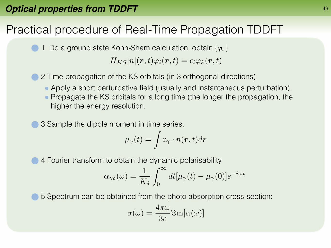
1 Do a ground state Kohn-Sham calculation: obtain {𝜑i }

2 Time propagation of the KS orbitals (in 3 orthogonal directions) Apply a short perturbative field (usually and instantaneous perturbation). Propagate the KS orbitals for a long time (the longer the propagation, the higher the energy resolution.

3 Sample the dipole moment in time series.

4 Fourier transform to obtain the dynamic polarisability

5 Spectrum can be obtained from the photo absorption cross-section:

�(!) =4⇡!

3c=m[↵(!)]

µ�(t) =

Zr� · n(r, t)dr

↵��(!) =1

K�

Z 1

0dt[µ�(t)� µ�(0)]e

�i!t

HKS [n](r, t)'i(r, t) = ✏i'k(r, t)


0 5000 10000 15000 20000

Tim

e de

pend

ent d

ipol

e m

omen

t

Time (hbar/eV)

x

0 5000 10000 15000 20000

Tim

e de

pend

ent d

ipol

e m

omen

t

Time (hbar/eV)

y

0 5000 10000 15000 20000

Tim

e de

pend

ent d

ipol

e m

omen

t

Time (hbar/eV)

z

x

y



0 5 10 15 20

Phot

oabs

ortio

n cr

oss-

sect

ion

ω (eV)

x

0 5 10 15 20

Phot

oabs

ortio

n cr

oss-

sect

ion

ω (eV)

y

0 5 10 15 20

Phot

oabs

ortio

n cr

oss-

sect

ion

ω (eV)

z

0 5 10 15 20

Phot

oabs

ortio

n cr

oss-

sect

ion

ω (eV)

TD-Propogation



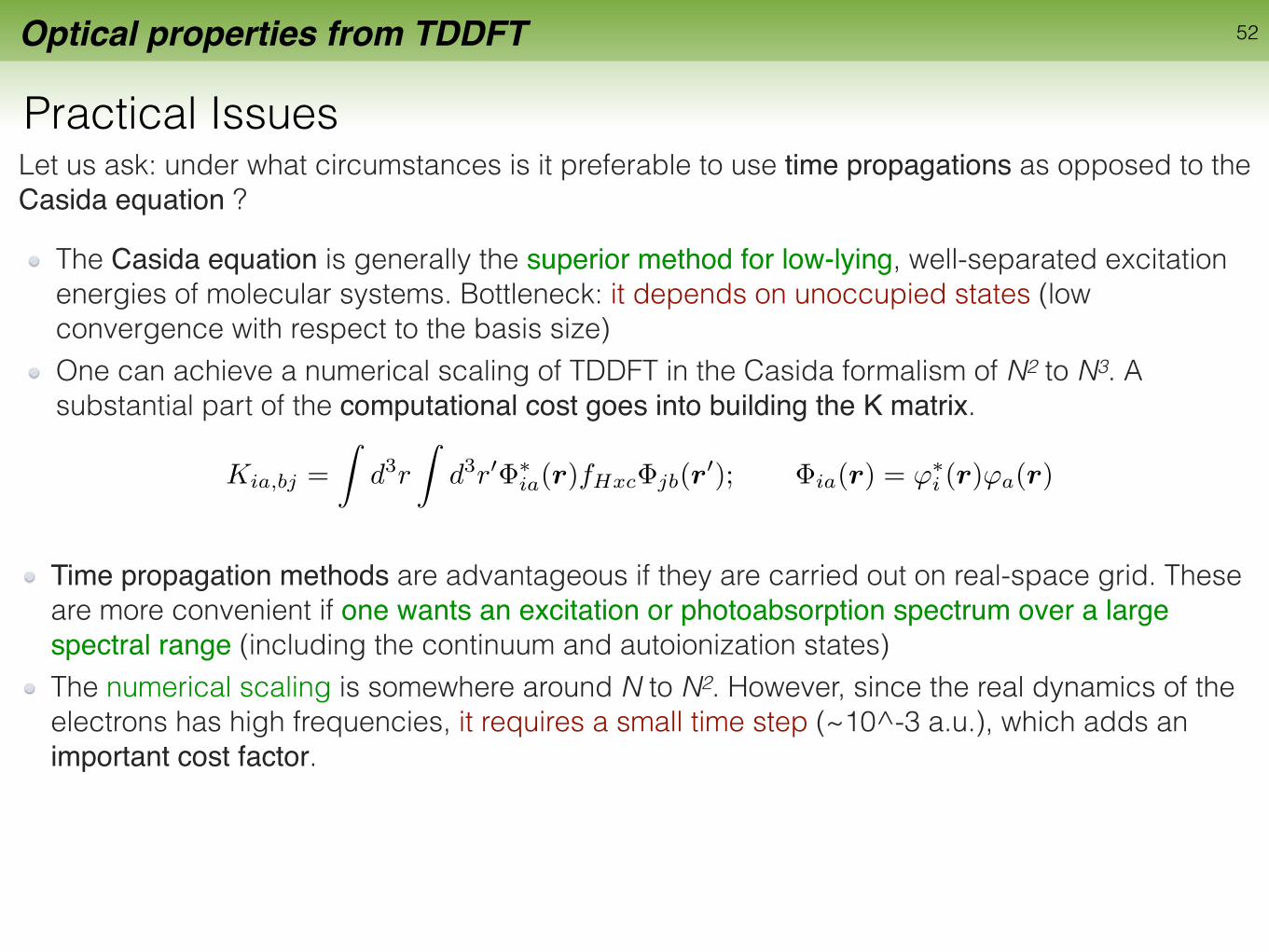
Practical IssuesLet us ask: under what circumstances is it preferable to use time propagations as opposed to the Casida equation ?

Time propagation methods are advantageous if they are carried out on real-space grid. These are more convenient if one wants an excitation or photoabsorption spectrum over a large spectral range (including the continuum and autoionization states) The numerical scaling is somewhere around N to N2. However, since the real dynamics of the electrons has high frequencies, it requires a small time step (~10^-3 a.u.), which adds an important cost factor.

The Casida equation is generally the superior method for low-lying, well-separated excitation energies of molecular systems. Bottleneck: it depends on unoccupied states (low convergence with respect to the basis size) One can achieve a numerical scaling of TDDFT in the Casida formalism of N2 to N3. A substantial part of the computational cost goes into building the K matrix.

Kia,bj =

Zd3r

Zd3r0�⇤

ia(r)fHxc�jb(r0); �ia(r) = '⇤

i (r)'a(r)

Outline 53





Some known failures of the TDDFT 54

Charge-Transfer (CT) ProblemCurrent xc-functionals usually underestimate dramatically charge transfer excitation state energies.Charge transfer according to IUPAC An electronic transition in which a large fraction of an electronic charge is transferred from one region of a molecular entity, called the electron donor, to another, called the electron acceptor (intramolecular CT) or from one molecular entity to another (intermolecular CT).


Charge-Transfer (CT) ProblemCurrent xc-functionals usually underestimate dramatically charge transfer excitation state energies.

Failure of Time-Dependent Density Functional Theory forLong-Range Charge-Transfer Excited States: The

Zincbacteriochlorin-Bacteriochlorin andBacteriochlorophyll-Spheroidene Complexes

Andreas Dreuw*,† and Martin Head-Gordon‡

Contribution from the Institut fur Physikalische und Theoretische Chemie, Johann WolfgangGoethe-UniVersitat Frankfurt, Marie-Curie-Strasse 11, 60439 Frankfurt, Germany,

and Department of Chemistry, UniVersity of California, Berkeley, and Chemical Scienceand Physical Bioscience DiVision, Lawrence Berkeley National Laboratory,

Berkeley, California 94720-1470

Received November 12, 2003; E-mail: [email protected]

Abstract: It is well-known that time-dependent density functional theory (TDDFT) yields substantial errorsfor the excitation energies of charge-transfer (CT) excited states, when approximate standard exchange-correlation (xc) functionals are used, for example, SVWN, BLYP, or B3LYP. Also, the correct 1/R asymptoticbehavior of CT states with respect to a distance coordinate R between the separated charges of the CTstate is not reproduced by TDDFT employing these xc-functionals. Here, we demonstrate by analysis ofthe TDDFT equations that the first failure is due to the self-interaction error in the orbital energies from theground-state DFT calculation, while the latter is a similar self-interaction error in TDDFT arising throughthe electron transfer in the CT state. Possible correction schemes, such as inclusion of exact Hartree-Fock or exact Kohn-Sham exchange, as well as aspects of the exact xc-functional are discussed in thiscontext. Furthermore, a practical approach is proposed which combines the benefits of TDDFT andconfiguration interaction singles (CIS) and which does not suffer from electron-transfer self-interaction.The latter approach is applied to a (1,4)-phenylene-linked zincbacteriochlorin-bacteriochlorin complex andto a bacteriochlorophyll-spheroidene complex, in which CT states may play important roles in energy andelectron-transfer processes. The errors of TDDFT alone for the CT states are demonstrated, and reasonableestimates for the true excitation energies of these states are given.

1. IntroductionTime-dependent density functional theory (TDDFT)1,2 has

become one of the most popular quantum chemical approachesfor calculating electronic spectra of medium-sized and largemolecules up to 200 second-row atoms (see, for example, refs3-6). Although TDDFT reaches the accuracy of sophisticatedquantum chemical methods for valence-excited states, whichare energetically well below the first ionization potential, itscomputational cost is remarkably low. In present-day TDDFT,one relies on the so-called adiabatic approximation,1,2 andapproximate ground-state exchange-correlation (xc) functionalsare applied.7-10

One major drawback of these approximate xc-functionals isthat the corresponding potentials do not exhibit the correct 1/rasymptotic behavior, where r is the electron-nucleus distance,11but fall off too rapidly.12 Also, for many xc-functionals, thecorresponding xc-potential is too high in the inner regions,resulting in underbound virtual orbitals.11,13 This leads, forinstance, to substantial errors for the excitation energies ofRydberg states in which the electron travels far away from thenucleus. Today, it is known that this failure can be compensatedby using asymptotically corrected potentials such as LB94.14However, it has been pointed out recently that TDDFT alsogives substantial errors for excited states of molecules withextended π-systems15,16 as well as for charge-transfer (CT)states.6,17,18 Especially, excitation energies of long-range CTstates in weakly interacting molecular complexes are drastically

† Johann Wolfgang Goethe-Universitat Frankfurt.‡ University of California, Berkeley and Lawrence Berkeley National

Laboratory.(1) Casida, M. E. In Recent AdVances in Density Functional Methods, Part I;

Chong, D. P., Ed.; World Scientific: Singapore, 1995.(2) Gross, E. U. K.; Dobson, J. F.; Petersilka, M. In Density Functional Theory

II; Nalewajski, R. F., Ed.; Springer: Heidelberg, 1996.(3) Sundholm, D. Chem. Phys. Lett. 1999, 302, 480.(4) Furche, F.; Ahlrichs, R.; Wachsmann, C.; Weber, E.; Sobanski, A.; Vogtle,

F.; Grimme, S. J. Am. Chem. Soc. 2000, 122, 1717.(5) Dreuw, A.; Dunietz, B. D.; Head-Gordon, M. J. Am. Chem. Soc. 2002,

124, 12070.(6) Dreuw, A.; Fleming, G. R.; Head-Gordon, M. J. Phys. Chem. B 2003, 107,

6500.(7) Dirac, P. A. M. Proc. Cambridge Philos. Soc. 1930, 26, 376.

(8) Vosko, S. H.; Wilk, L.; Nusair, M. Can. J. Phys. 1980, 58, 1200.(9) Becke, A. D. Phys. ReV. A 1988, 38, 3098.(10) Becke, A. D. J. Chem. Phys. 1993, 98, 5648.(11) Casida, M. E.; Jamorski, C.; Casida, K. C.; Salahub, D. R. J. Chem. Phys.

1998, 108, 4439.(12) Tozer, D. J.; Handy, N. C. J. Chem. Phys. 1998, 109, 10180.(13) Casida, M. E.; Casida, K. C.; Salahub, D. R. Int. J. Quantum Chem. 1998,

70, 933.(14) van Leeuwen, R.; Baerends, E. J. Phys. ReV. A 1994, 49, 2421.(15) Cai, Z.-L.; Sendt, K.; Reimers, J. R. J. Chem. Phys. 2002, 117, 5543.(16) Grimme, S.; Parac, M. ChemPhysChem 2003, 3, 292.

Published on Web 03/06/2004

10.1021/ja039556n CCC: $27.50 © 2004 American Chemical Society J. AM. CHEM. SOC. 2004, 126, 4007-4016 9 4007



Exercise: Why does LR-TDDFT in AA fail to evaluate CT excitation energies?

Then, if the Adiabatic Approximation if applied to the exchange-correlation kernel, in both time and space domain ( ), the K matrix vanishes because the (i,a)-overlapping are zero.

fxc

(r, r0,!) ⇡ fxc

(r)�(r � r0)

One solution: include the Fock-exchange term into the kernel (i.e. hybrid functionals)

Aia,jb = �ia�jb(✏a � ✏i) + Jia,jb � cHFJij,ab + (1� cHF)K0ia,jb

Bia,jb = Jia,bj � cHFJib,aj + (1� cHF)K0ia,bj

notice that the only non-zero term is due to the HF exact exchange term of the A matrix. All other terms are zero because the orbitals i,j are localised on molecule 1, and a,b in molecule 2.

✓A BB⇤ A⇤

◆✓XY

◆= ⌦

✓�I 00 I

◆✓XY

◆

where the Hartree-exchange-correlation matrix elements are defined as

Kia,jb =

Zd3r

Zd3r0�⇤

ia(r)fHxc�jb(r0); �ia(r) = '⇤

i (r)'a(r)

Aia,jb = �ia�jb(✏a � ✏i) +Kia,jb

Bia,jb = Kia,bj



LE

LE

CT

CT

GGA+ALDA (BLYP) HYBRID: B3LYP

LUMO is generally more strongly bound in DFT, then the orbital energy difference corresponding to a CT state (pure TDDFT) is usually a drastic underestimation of its correct excitation energy.


Topology of the excited states What about the topology of the TDDFT PESs close to a conical intersection?

CI topology is characterised by the “branching space”

TDDFT: Topology of the excited state PESs

Photochemistry/photophysics require a correct description of the topological properties

of the most relevant potential energy surfaces involved.

Molecular geometries where two electronic

states are exactly degenerate

Sx

Sy

energ

y

gIJ

hij

Conical intersections are now recognized to play a critical role in the reaction dynamics of

electronic excited states.

define the direction that lift the degeneracy between the PESs.

- difference gradient,

- non-adiabatic coupling vectors

At a conical intersection two coordinates (over 3N):

difference gradient:

non-adiabatic coupling vector:

gij = rR(Ej � Ei)

hij = h i|rR| ji

Photochemistry/photophysics require a correct description of the topological properties of the most relevant potential energy surfaces involved. Conical intersections (CX) are now recognized to play a critical role in the reaction dynamics of electronic excited states.


Topology of the excited states What about the topology of the TDDFT PESs close to a conical intersection?

Photochemistry/photophysics require a correct description of the topological properties of the most relevant potential energy surfaces involved. Conical intersections (CX) are now recognized to play a critical role in the reaction dynamics of electronic excited states.

TDDFT: Topology of the excited state PESs

Photochemistry/photophysics require a correct description of the topological properties

of the most relevant potential energy surfaces involved.

Molecular geometries where two electronic

states are exactly degenerate

Sx

Sy

energ

y

gIJ

hij

Conical intersections are now recognized to play a critical role in the reaction dynamics of

electronic excited states.

define the direction that lift the degeneracy between the PESs.

- difference gradient,

- non-adiabatic coupling vectors

At a conical intersection two coordinates (over 3N):

gij = rR(Ej � Ei)

By applying Brillouin’s theorem, one can show that restricted CIS (for closed shell systems) has the wrong dimensionality for the intersection with the S0 PES: f − 1 (a seam of intersections instead of a conical intersection). Therefore, it is believed that CXs should not normally exist at the configuration interaction singles (CIS) level when the ground state is a closed-shell singlet

hij = h i|rR| ji = 0

Although the structure of the LR-TDDFT/TDA equations in the matrix formulation (Casida’s equations) is similar to CIS, the Brillouin’s theorem, does not hold in TDDFT and the question about the existence of CXs in DFT/LR- TDDFT remains open.


Topology of the excited states Concerning the coupling between S0 and S1, the main issue is to understand if LR-TDDFT in the usual approximations (adiabatic TDA with standard GGA functionals) can correctly predict the dimensionality of the intersection between the two surfaces.

Examples of LR-TDDFT calculations Some known failures

Topology of the excited states

S0/S1 intersection in linear water (Mol. Phys., 104, 1039 (2006))CIS - TDDFT

CASSCF

TDDFT for excitation energies

S0/S1 intersection in linear water (Mol. Phys., 104, 1039 (2006))

Some examples:



S0/S1 intersection in linear water (Mol. Phys., 104, 1039 (2006))CIS - TDDFT

CASSCF


Usual approximation of TDDFT fails on the CI description.

CIS TDDFT CASSCF



S0/S1 for H2 + H (Mol. Phys., 104, 1039 (2006))

TDDFT - CASSCF

TDDFT seems to reproduce the correct splitting of the surfaces.However, slope around the CI is much steeper...




S0/S1 for H2 + H (Mol. Phys., 104, 1039 (2006))

Some examples:

TDDFT CASSCF

Usual approximation of TDDFT gives a qualitatively description of the CI (slope around the CI is much steeper )


Concerning the coupling between S0 and S1, the main issue is to understand if LR-TDDFT in the usual approximations (adiabatic TDA with standard GGA functionals) can correctly predict the dimensionality of the intersection between the two surfaces.



S0/S1 for C2H4O (J. Chem. Phys. 129, 124108 (2008) )

Some examples:

TDDFT CASSCF

but it is not always the case !!!



... but it is not a general failure of TDDFT

Ref: J. Chem. Phys. 129, 124108 (2008).




... but it is not a general failure of TDDFT

Ref: J. Chem. Phys. 129, 124108 (2008).



Concerning the coupling between S0 and S1, the main issue is to understand if LR-TDDFT in the usual approximations (adiabatic TDA with standard GGA functionals) can correctly predict the dimensionality of the intersection between the two surfaces.

Short-Summary for LR-TDDFT for Excitation energies 63

For valence excited states well below the ionization potential—> error between 0.2 and 0.6 eV (0.1 eV ≈ 10 kJ/mol). Good ordering and relative energies of the excited states (except for CT states). Good also for transition metals (difficult for wavefunction based methods).

Scales ∼ like O(n2) with n the number of electrons: can deal with very large systems up to many hundreds of atoms.

Many times, TDDFT properties are bad because the underlying DFT is inaccurate (bond dissociations, biradicals, self-interaction error, . . . ). Topology of the excited surfaces is not always correct. Problems to describe double excitations, Rydberg excited states, large π systems. Standard xc functionals fail in the case of CT states.Errors in the ordering of the excited PESs is deleterious for excited states MD.

Applicability of TDDFT

REFERENCES 64

Main References used in this lecture:

• Fundamentals of Time-Dependent Density Functional TheoryEditors: Marques, M.A.L., Maitra, N.T., Nogueira, F.M.S., Gross, E.K.U., Rubio, A. (Eds.).

• Time-dependent density-functional theory : concepts and applications Author:Carsten Ullrich Publisher: Oxford ; New York : Oxford University Press, 2012.

• TDDFT for excitation energies: TDDFT for ultrafast electronic dynamicsIvano Tavernelli and Basile Curchod. (http://benasque.org/2014tddft/talks_contr/103_Ivano1.pdf)

• Time Dependent Density Functional Response Theory for MoleculesMark E. Casida . Recent Advances in Density Functional Methods: pp. 155-192.(1995). DOI: http://dx.doi.org/10.1142/9789812830586_0005

http://benasque.org/2014tddft/talks_contr/103_Ivano1.pdf

http://dx.doi.org/10.1142/9789812830586_0005

applied tddft - i: a chemist’s...

Documents