Time-dependent Density Functional Theory

in GPAWTool for Exploring Excited State Properties

Lauri Lehtovaaralauri.lehtovaara@hut.fi

Helsinki University of Technology

Outline for Part I: Theory

● Time-dependent DFT● Time propagation TDDFT● TDDFT in GPAW● Examples

– Linear absorption spectrum

– Nonlinear emission spectrum

● Implementation● More examples● Summary

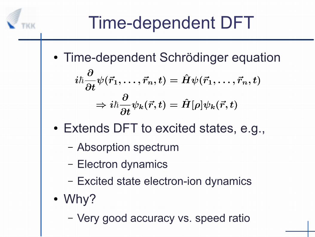
Time-dependent DFT

● Time-dependent Schrödinger equation

● Extends DFT to excited states, e.g.,– Absorption spectrum

– Electron dynamics

– Excited state electron-ion dynamics

● Why?– Very good accuracy vs. speed ratio

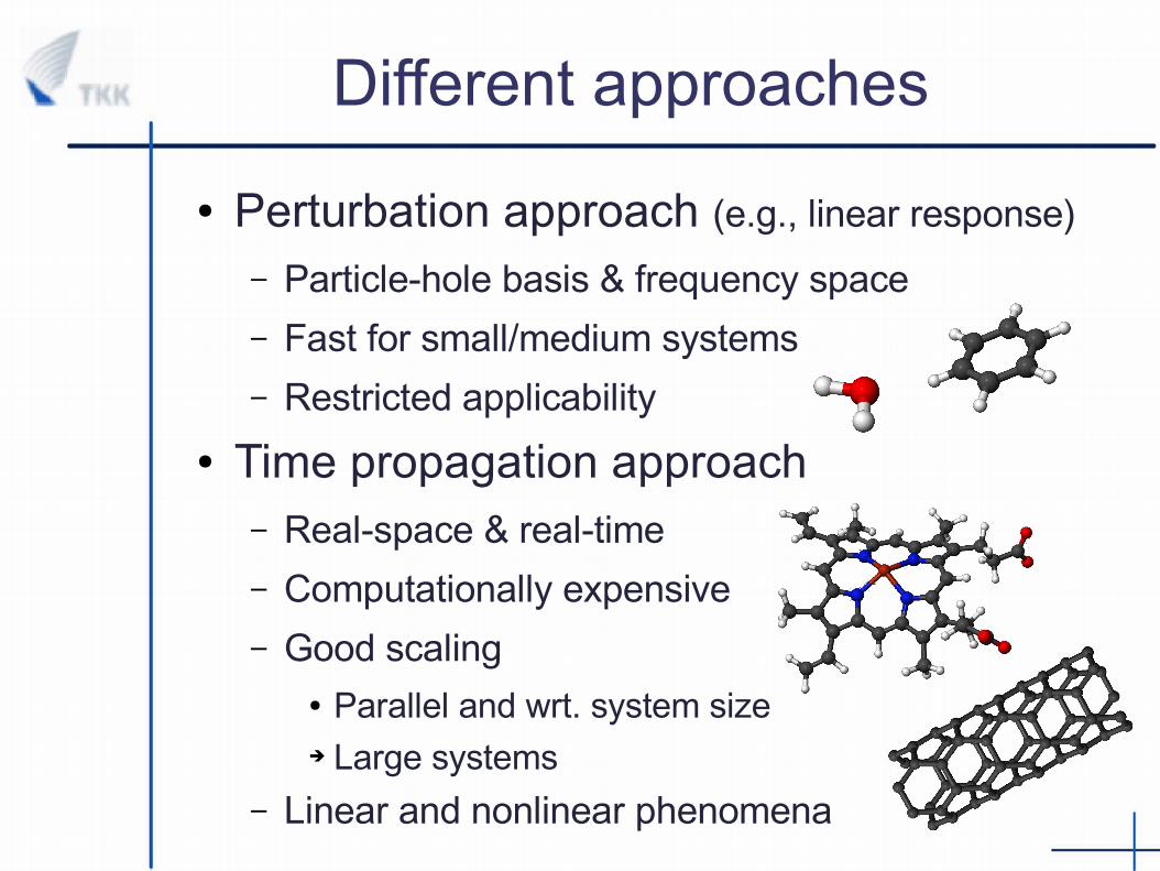
Different approaches

● Perturbation approach (e.g., linear response)

– Particle-hole basis & frequency space

– Fast for small/medium systems

– Restricted applicability

● Time propagation approach– Real-space & real-time

– Computationally expensive

– Good scaling● Parallel and wrt. system size➔ Large systems

– Linear and nonlinear phenomena

GPAW

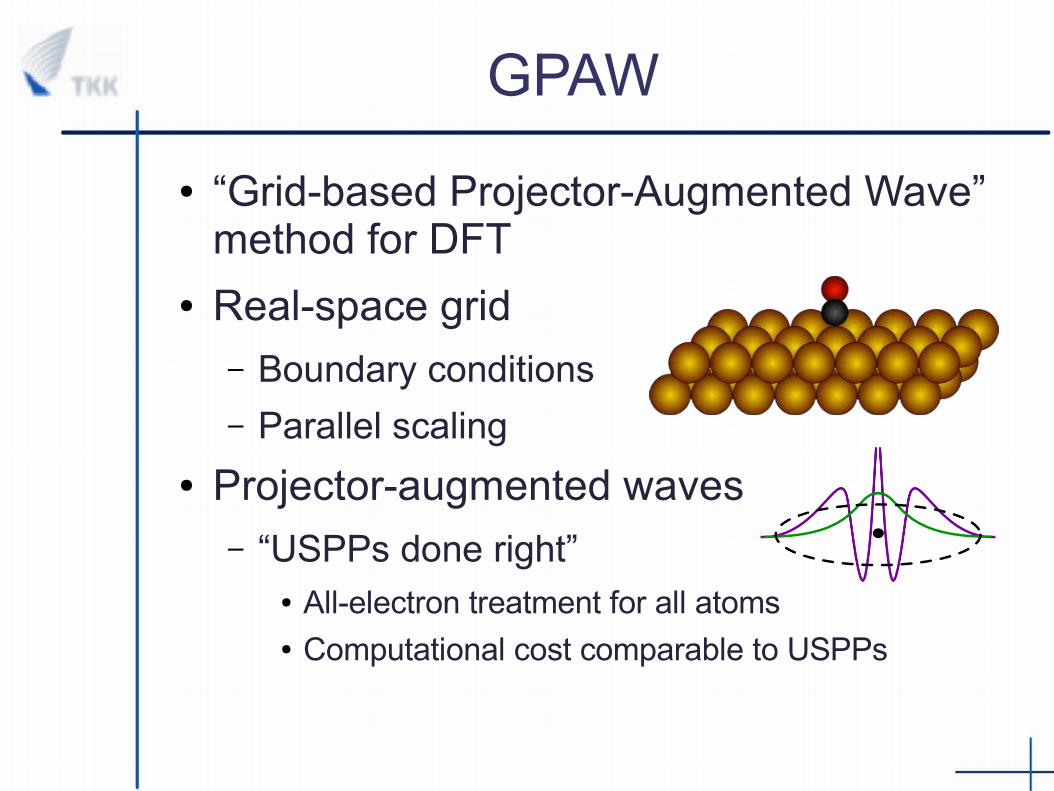
● “Grid-based Projector-Augmented Wave” method for DFT

● Real-space grid– Boundary conditions

– Parallel scaling

● Projector-augmented waves– “USPPs done right”

● All-electron treatment for all atoms● Computational cost comparable to USPPs

TDDFT in GPAW

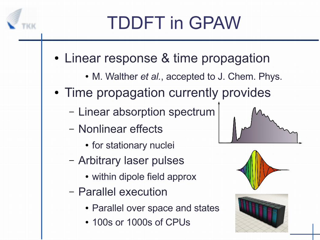
● Linear response & time propagation● M. Walther et al., accepted to J. Chem. Phys.

● Time propagation currently provides– Linear absorption spectrum

– Nonlinear effects● for stationary nuclei

– Arbitrary laser pulses● within dipole field approx

– Parallel execution● Parallel over space and states● 100s or 1000s of CPUs

Example: Absorption spectrum

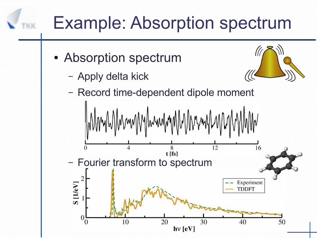
● Absorption spectrum– Apply delta kick

– Record time-dependent dipole moment

– Fourier transform to spectrum

Example: Harmonic generation

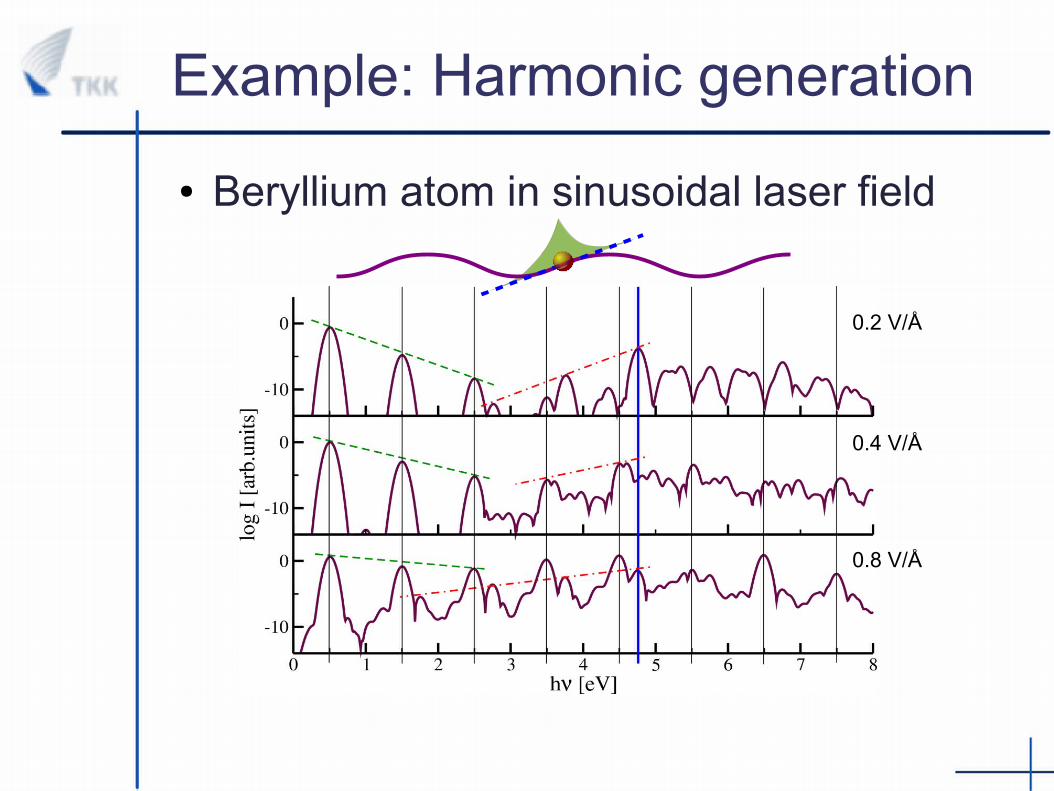
● Beryllium atom in sinusoidal laser field

0.2 V/Å

0.4 V/Å

0.8 V/Å

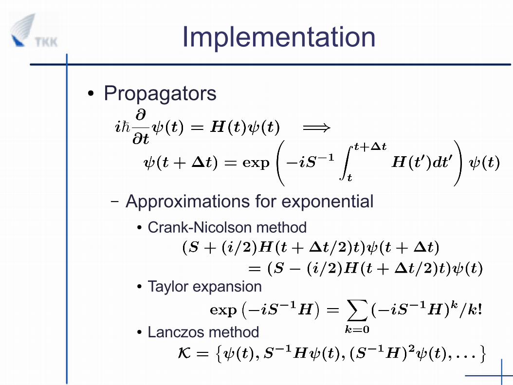
Implementation

● Propagators

– Approximations for exponential● Crank-Nicolson method

● Taylor expansion

● Lanczos method

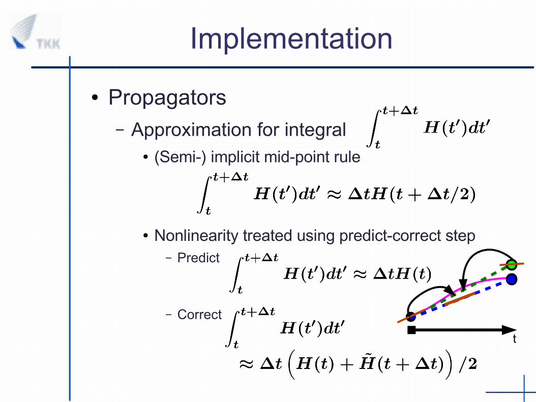
Implementation

● Propagators– Approximation for integral

● (Semi-) implicit mid-point rule

● Nonlinearity treated using predict-correct step– Predict

– Correct

t

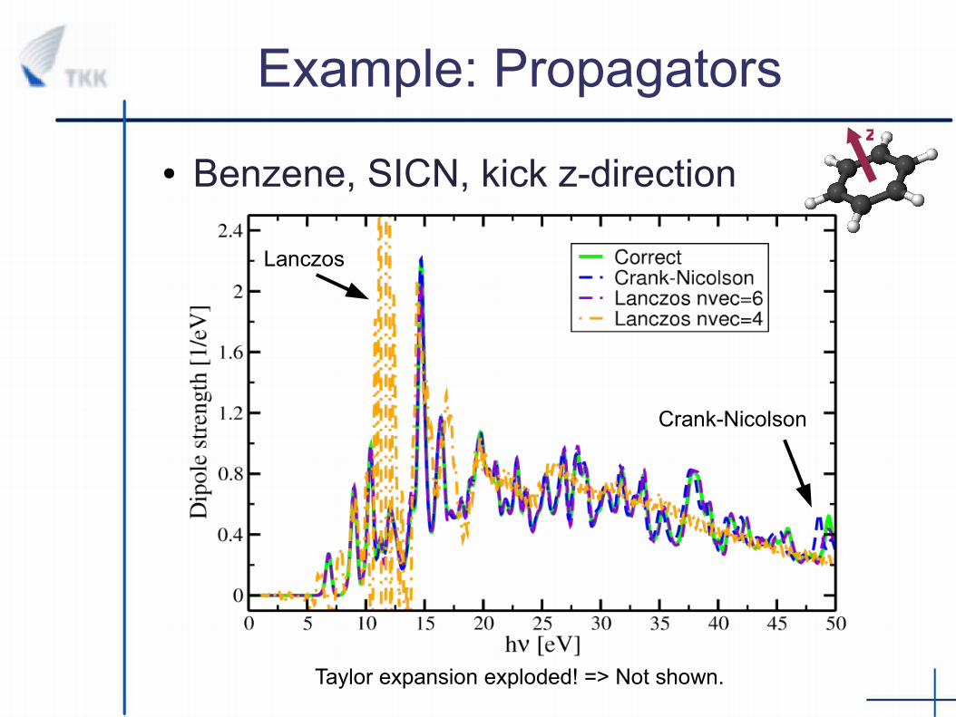
Example: Propagators

● Benzene, SICN, kick z-directionz

Lanczos

Crank-Nicolson

Taylor expansion exploded! => Not shown.

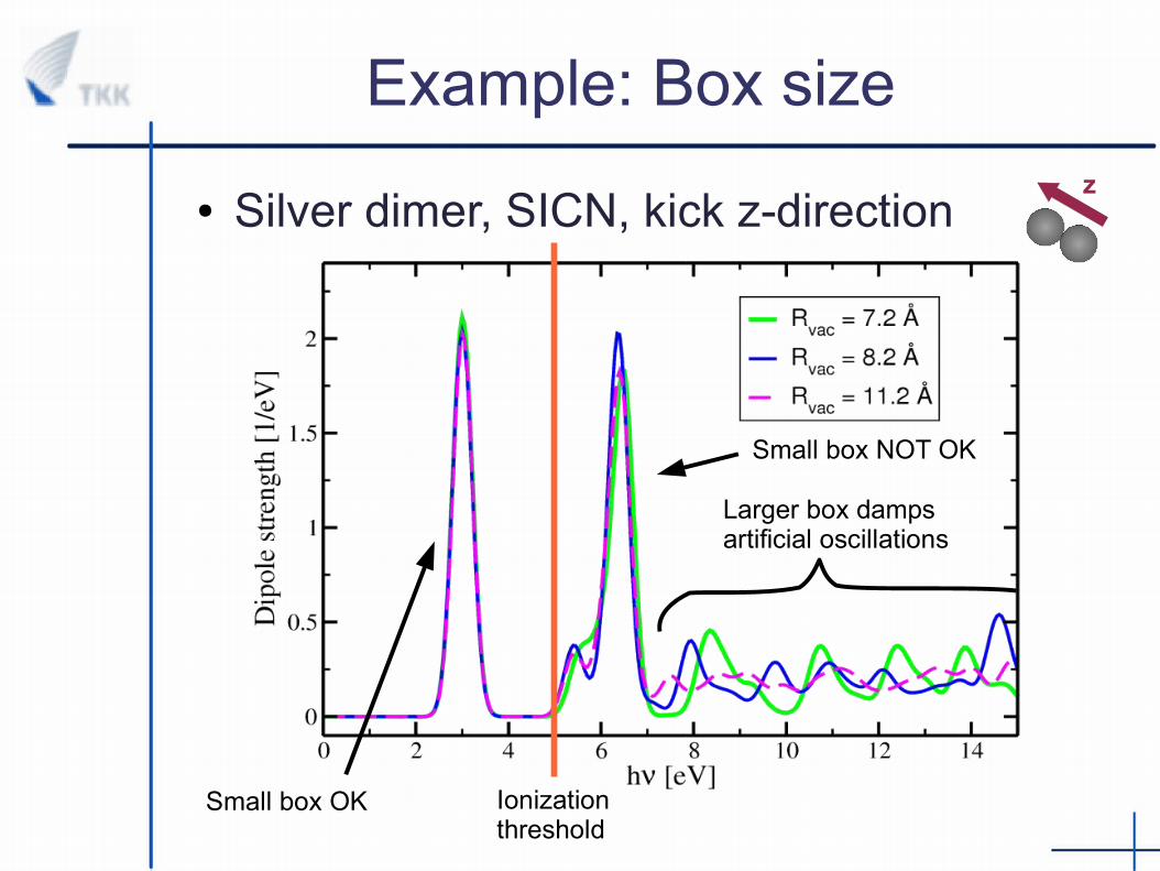
Example: Box size

● Silver dimer, SICN, kick z-directionz

Ionizationthreshold

Small box OK

Small box NOT OK

Larger box damps artificial oscillations

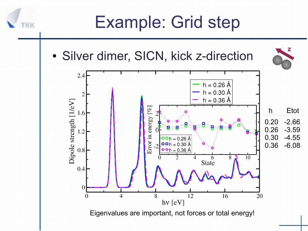
Example: Grid step

● Silver dimer, SICN, kick z-directionz

Eigenvalues are important, not forces or total energy!

h Etot

0.20 -2.660.26 -3.59 0.30 -4.55 0.36 -6.08

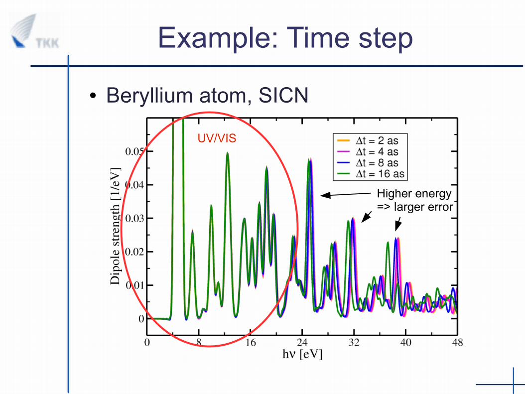
Example: Time step

● Beryllium atom, SICN

UV/VIS

Higher energy=> larger error

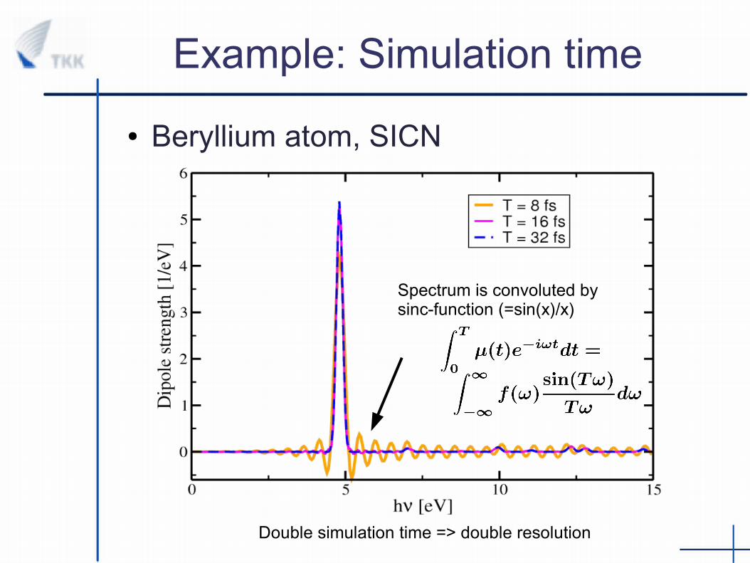
Example: Simulation time

● Beryllium atom, SICN

Spectrum is convoluted bysinc-function (=sin(x)/x)

Double simulation time => double resolution

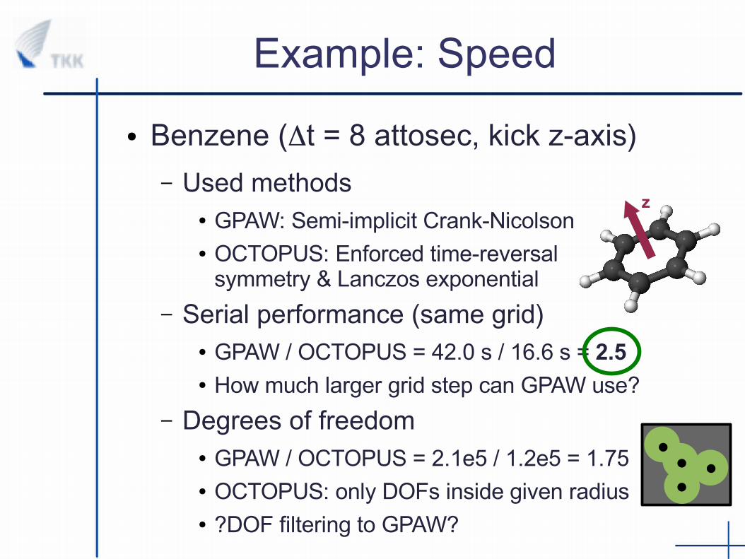
Example: Speed

● Benzene (Δt = 8 attosec, kick z-axis)

– Used methods● GPAW: Semi-implicit Crank-Nicolson● OCTOPUS: Enforced time-reversal

symmetry & Lanczos exponential

– Serial performance (same grid)● GPAW / OCTOPUS = 42.0 s / 16.6 s = 2.5● How much larger grid step can GPAW use?

– Degrees of freedom● GPAW / OCTOPUS = 2.1e5 / 1.2e5 = 1.75● OCTOPUS: only DOFs inside given radius● ?DOF filtering to GPAW?

z

1.8

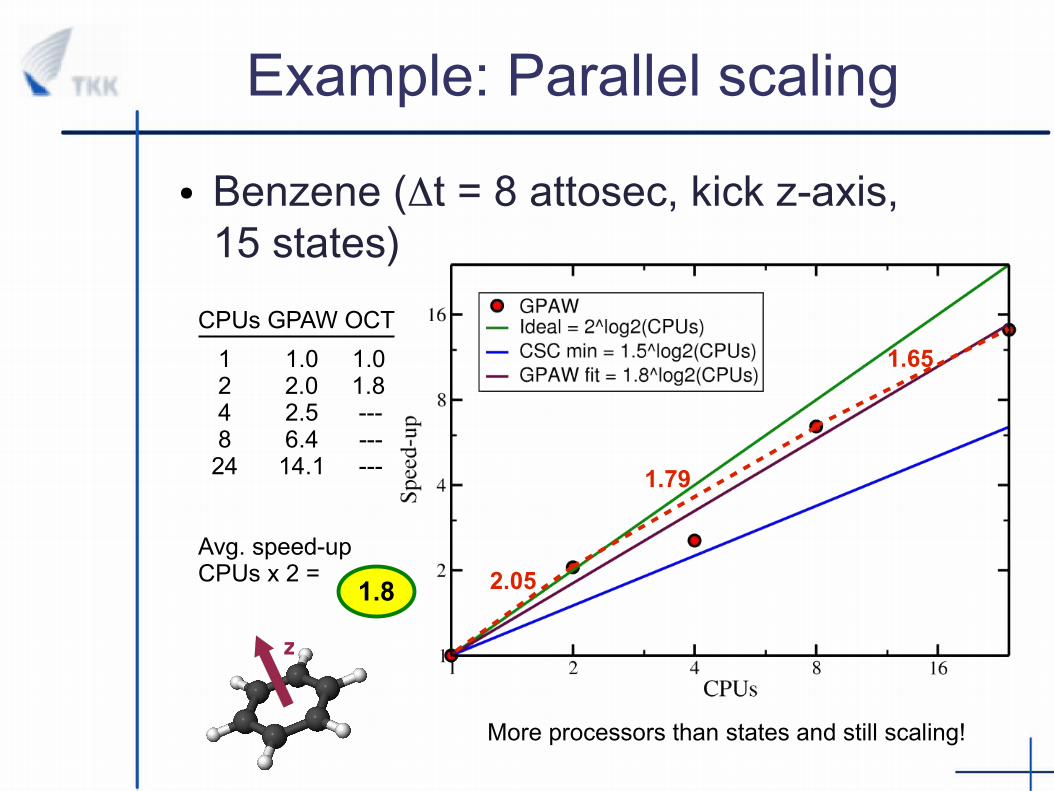
Example: Parallel scaling

● Benzene (Δt = 8 attosec, kick z-axis, 15 states)

z

CPUs GPAW OCT

1 1.0 1.0 2 2.0 1.8 4 2.5 --- 8 6.4 --- 24 14.1 ---

Avg. speed-upCPUs x 2 =

More processors than states and still scaling!

1.65

1.79

2.05

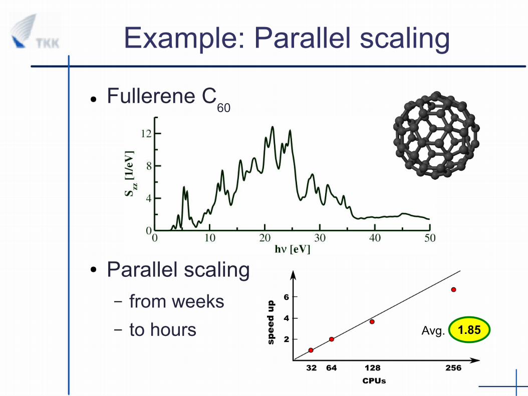
Example: Parallel scaling

● Fullerene C60

● Parallel scaling– from weeks

– to hours Avg. 1.85

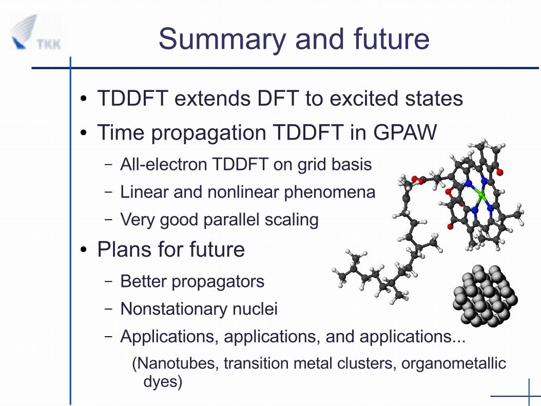
Summary and future

● TDDFT extends DFT to excited states● Time propagation TDDFT in GPAW

– All-electron TDDFT on grid basis

– Linear and nonlinear phenomena

– Very good parallel scaling

● Plans for future– Better propagators

– Nonstationary nuclei

– Applications, applications, and applications...

(Nanotubes, transition metal clusters, organometallic dyes)

Outline for Part II: Practice

● Ground state for TDDFT● Hands-on example: Na2 spectrum

– Ground state script

– TDDFT script

– Run script in Murska

● Example: C60– Python script

– Parallel-over-states run script

● Example: Laser pulse

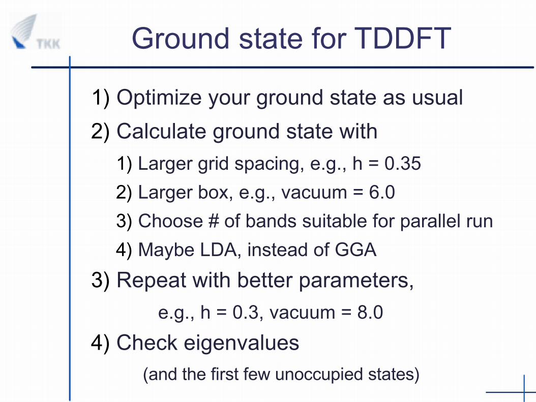
Ground state for TDDFT

1) Optimize your ground state as usual

2) Calculate ground state with

1) Larger grid spacing, e.g., h = 0.35

2) Larger box, e.g., vacuum = 6.0

3) Choose # of bands suitable for parallel run

4) Maybe LDA, instead of GGA

3) Repeat with better parameters,

e.g., h = 0.3, vacuum = 8.0

4) Check eigenvalues(and the first few unoccupied states)

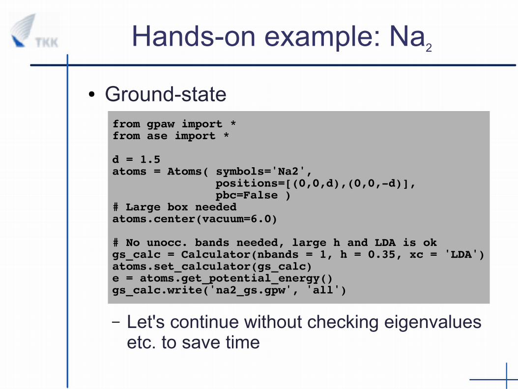
Hands-on example: Na2

● Ground-state

– Let's continue without checking eigenvalues etc. to save time

from gpaw import *from ase import *

d = 1.5atoms = Atoms( symbols='Na2', positions=[(0,0,d),(0,0,-d)], pbc=False )# Large box neededatoms.center(vacuum=6.0)

# No unocc. bands needed, large h and LDA is okgs_calc = Calculator(nbands = 1, h = 0.35, xc = 'LDA')atoms.set_calculator(gs_calc)e = atoms.get_potential_energy()gs_calc.write('na2_gs.gpw', 'all')

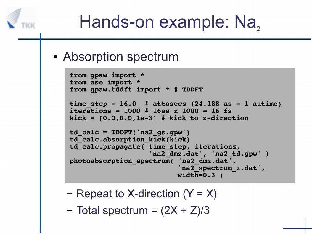
Hands-on example: Na2

● Absorption spectrum

– Repeat to X-direction (Y = X)

– Total spectrum = (2X + Z)/3

from gpaw import *from ase import *from gpaw.tddft import * # TDDFT

time_step = 16.0 # attosecs (24.188 as = 1 autime)iterations = 1000 # 16as x 1000 = 16 fskick = [0.0,0.0,1e-3] # kick to z-direction

td_calc = TDDFT('na2_gs.gpw')td_calc.absorption_kick(kick)td_calc.propagate( time_step, iterations, 'na2_dmz.dat', 'na2_td.gpw' ) photoabsorption_spectrum( 'na2_dmz.dat', 'na2_spectrum_z.dat', width=0.3 )

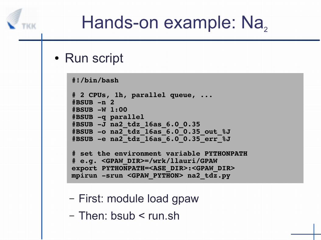
Hands-on example: Na2

● Run script

– First: module load gpaw

– Then: bsub < run.sh

#!/bin/bash

# 2 CPUs, 1h, parallel queue, ...#BSUB -n 2#BSUB -W 1:00#BSUB -q parallel#BSUB -J na2_tdz_16as_6.0_0.35#BSUB -o na2_tdz_16as_6.0_0.35_out_%J#BSUB -e na2_tdz_16as_6.0_0.35_err_%J

# set the environment variable PYTHONPATH # e.g. <GPAW_DIR>=/wrk/llauri/GPAWexport PYTHONPATH=<ASE_DIR>:<GPAW_DIR>mpirun -srun <GPAW_PYTHON> na2_tdz.py

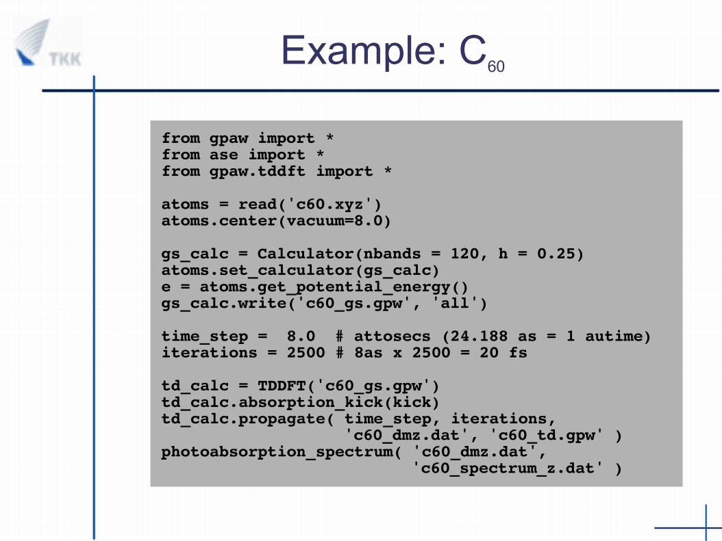
Example: C60

from gpaw import *from ase import *from gpaw.tddft import *

atoms = read('c60.xyz')atoms.center(vacuum=8.0)

gs_calc = Calculator(nbands = 120, h = 0.25)atoms.set_calculator(gs_calc)e = atoms.get_potential_energy()gs_calc.write('c60_gs.gpw', 'all')

time_step = 8.0 # attosecs (24.188 as = 1 autime)iterations = 2500 # 8as x 2500 = 20 fs

td_calc = TDDFT('c60_gs.gpw')td_calc.absorption_kick(kick)td_calc.propagate( time_step, iterations, 'c60_dmz.dat', 'c60_td.gpw' ) photoabsorption_spectrum( 'c60_dmz.dat', 'c60_spectrum_z.dat' )

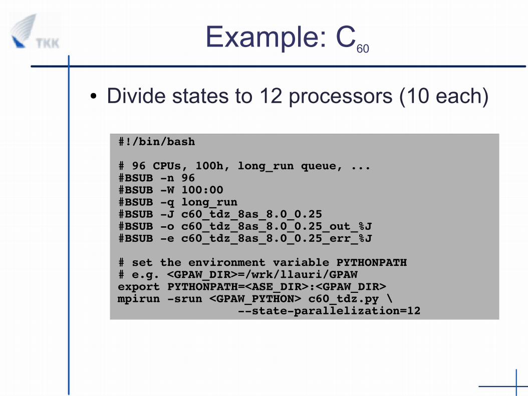
Example: C60

● Divide states to 12 processors (10 each)

#!/bin/bash

# 96 CPUs, 100h, long_run queue, ...#BSUB -n 96#BSUB -W 100:00#BSUB -q long_run#BSUB -J c60_tdz_8as_8.0_0.25#BSUB -o c60_tdz_8as_8.0_0.25_out_%J#BSUB -e c60_tdz_8as_8.0_0.25_err_%J

# set the environment variable PYTHONPATH # e.g. <GPAW_DIR>=/wrk/llauri/GPAWexport PYTHONPATH=<ASE_DIR>:<GPAW_DIR>mpirun -srun <GPAW_PYTHON> c60_tdz.py \

--state-parallelization=12

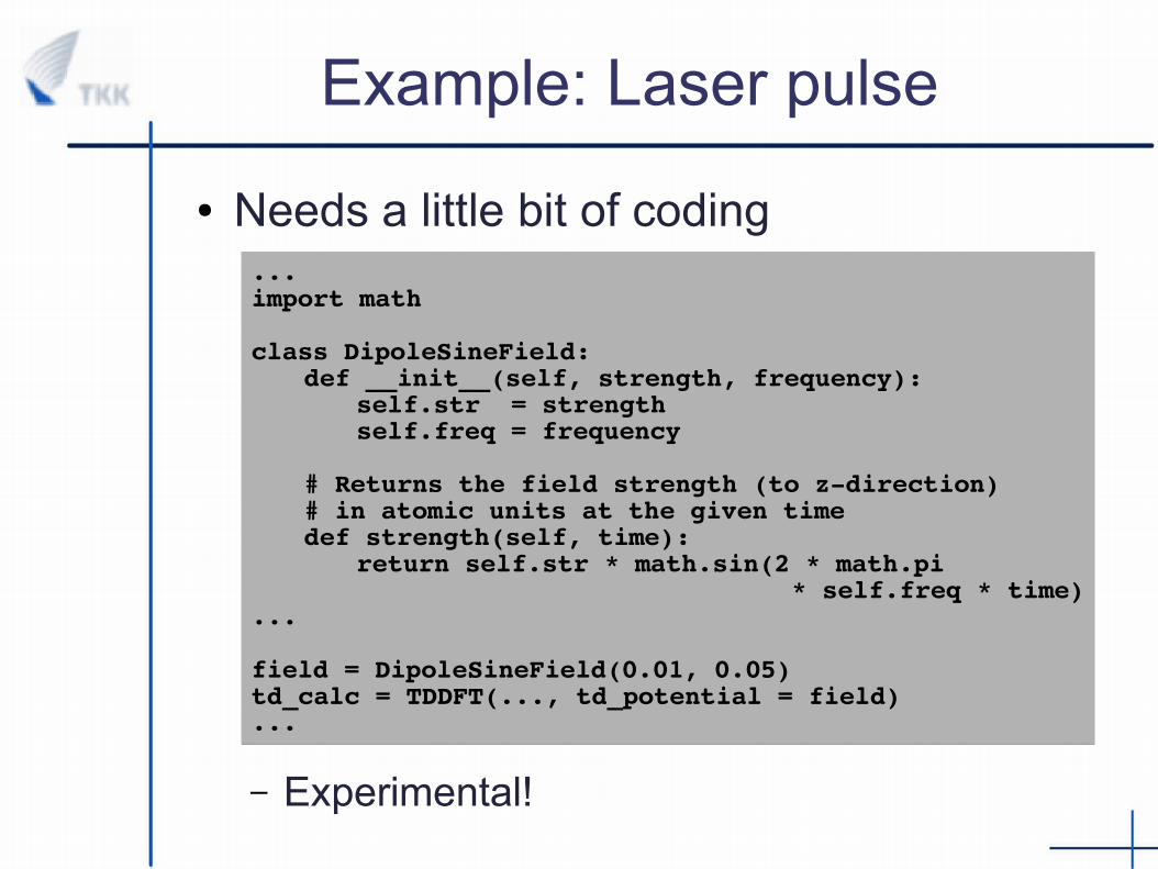
Example: Laser pulse

● Needs a little bit of coding

– Experimental!

...import math

class DipoleSineField:def __init__(self, strength, frequency): self.str = strength

self.freq = frequency

# Returns the field strength (to z-direction)# in atomic units at the given timedef strength(self, time):

return self.str * math.sin(2 * math.pi * self.freq * time)...

field = DipoleSineField(0.01, 0.05)td_calc = TDDFT(..., td_potential = field)...

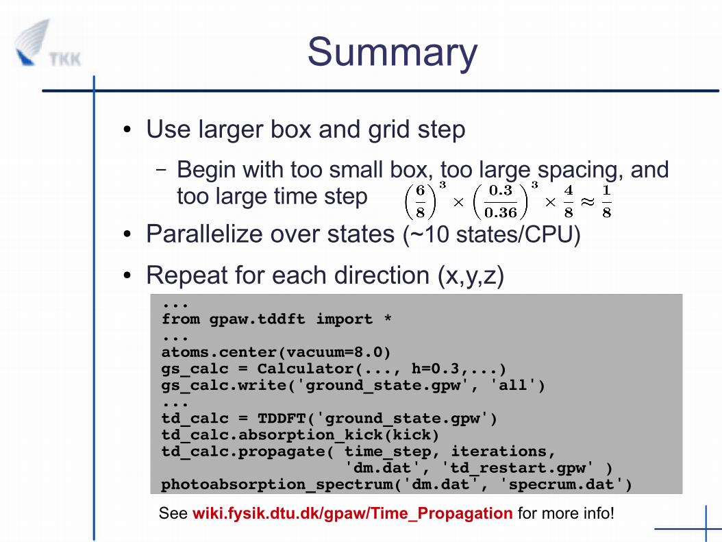
Summary

● Use larger box and grid step

– Begin with too small box, too large spacing, and too large time step

● Parallelize over states (~10 states/CPU)

● Repeat for each direction (x,y,z)...from gpaw.tddft import *...atoms.center(vacuum=8.0)gs_calc = Calculator(..., h=0.3,...)gs_calc.write('ground_state.gpw', 'all') ...td_calc = TDDFT('ground_state.gpw')td_calc.absorption_kick(kick)td_calc.propagate( time_step, iterations, 'dm.dat', 'td_restart.gpw' )photoabsorption_spectrum('dm.dat', 'specrum.dat')

See wiki.fysik.dtu.dk/gpaw/Time_Propagation for more info!