application of machine learning models in predicting

29-40

29

The Mining-Geology-Petroleum Engineering BulletinUDC: 622.3:553.9DOI: 10.17794/rgn.2019.3.4

Preliminary communication

Corresponding author: Princewill Maduabuchi [email protected]

Application of machine learning models in predicting initial gas production rate from tight gas reservoirs

Ugwumba Chrisangelo Amaechi1; Princewill Maduabuchi Ikpeka2; Ma Xianlin1; Johnson Obunwa Ugwu3

1Oil and Gas Field Development Engineering, Xi’An Shiyou University, China2Department of Petroleum Engineering, Federal University of Technology, Owerri, Nigeria3 School of Science, Engineering and Design, Teesside University, United Kingdom

AbstractDriven by advancements in technology, tight-gas fi eld development has become a signifi cant source of hydrocarbon to the energy industry. The amount of data generated in the process is immense as most platforms are now being digitized. Machine learning tools can be used to analyse this data in order to build patterns between several dependent and inde-pendent variables. Forecasting initial gas production rates has important implications in the planning production/pro-cessing facilities for new wells, aff ects investment decisions and is an important component of reporting to regulatory agencies. This study is based on the analysis of reservoir rock/fl uid properties and selected well parameters to build de-cision-based models that can predict initial gas production rates for tight gas formations. In this study, two machine learning predictive models; Artifi cial Neural Network (ANN) and Generalized Linear Model (GLM), were used to deter-mine the expected recovery rate of planned new wells. Production data was retrieved from 224 wells and used in develop-ing the model. The results obtained from these models were then compared to the actual recorded initial gas production rate from the wells. Results from the analysis carried out revealed a Mean Square Error (MSE) of 1.57 on a GLM model whereas the ANN model gave an MSE of 1.24. Key Performance Index for the ANN model revealed that reservoir thick-ness had the highest (36.5%) contribution to the initial gas production rate followed by the fl owback rate (29%). The reservoir/fl uid properties contribution to the initial gas production rate was 53% while the hydraulic fracture parameters contribution to the initial gas production rate was 47%.

Keywords:predictive analytics; machine learning; artifi cial neural network; initial gas production rate; look-back analysis

1. Introduction

As technological advancements continue to improve daily in the oil and gas sector, spurred by advancements in shale oil and gas development, smart fi eld develop-ment, cheaper and more reliable data storage technolo-gies have led to an increase in the amount of data cap-tured in the industry. For example, in developing tight gas formations, hydraulic fracturing is used to produce fractures in rock formations which stimulate the fl ow of natural gas. Reservoir modelling in such systems is an extremely complicated task, given the need to simulate fl uid fl ow in a network of induced natural fractures cou-pled to geo-mechanical effects and other processes such as water blocking, non-Darcy fl ow in nano-scale pores, and adsorption/desorption (Cipolla et al., 2010 and Ding et al., 2014). Tight gas refers to natural gas trapped in a reservoir with a matrix permeability lower than 0.1×10-3 μm2, which usually has no natural deliverability

or lower natural deliverability than the industrial stand-ard, so stimulation or special treatment wells must be used to obtain commercial gas fl ow. (National Energy Administration, 2011). Tight gas reservoirs can be di-vided into two types based on reservoir characteristics, reserves, and structural positions; Continuous-type and Trap-type tight gas reservoirs (Da et al., 2012).

Oil and gas production companies use thousands of sensors installed in the subsurface and surface facilities to provide continuous data collection, real-time monitor-ing of assets and the environmental conditions (Ab-delkadir and Luc, 2014). This data comes in structured, semi-structured and unstructured forms. According to Gupta (2016), analytics reveal patterns and relation-ships in this data in order to improve decision making. Analytical techniques are used to identify patterns in historical and even specifi c data which can then be cor-related to current or future data to identify risk and op-portunities (Bravo et al. 2014). Machine learning in re-cent times has been successfully employed in different fi elds where huge amounts of data are prevalent to gen-

Amaechi, U.C.; Ikpeka, P.M.; Xianin, M.; Ugwu J.O. 30

The Mining-Geology-Petroleum Engineering Bulletin and the authors ©, 2019, pp. 29-40, DOI: 10.17794/rgn.2019.3.4

erate data driven models for operation and business de-cision making purposes (Hastie et al. 2001).

The use of neural networks in data analysis is not new to the petroleum industry. Malvić and Prskalo (2007) applied a back propagation neural network in the pro-cessing of three seismic attributes: amplitude, phase and frequencies from 14 wells. The results were subsequent-ly used to predict reservoir porosity. Cvetković et al. (2009) used two types of neural networks: supervised learning-multilayer perceptron and the radial basis func-tion neural network to successfully predict the lithology and the hydrocarbon saturation of the Upper Pannonian sediments and Lower Pontian deposits in the Kloštar fi eld. Malvić et al (2010) utilized supervised neural al-gorithms for well log and seismic data analysis in three fi elds. The algorithms used in their work mainly consist of multi-layer perceptron architecture and the activation function used was sigmoid or log-sigmoid. However, a radial basis function was also used as an activation func-tion for one network. This implies that different types of back propagation architecture and activation can be used. Šapina (2016) in his work made an interesting comparison between mapping using artifi cial neural net-work (ANN) and the ordinary kriging method. Although from his work, the ordinary kriging method had a lower mean square error, this was attributed mainly to the fact

that ANN utilized a relatively small amount of data in comparison with kriging.

In this paper, machine learning is used to generate data driven models for business operational and business decision purposes in the oil and gas sector especially in the unconventional reservoirs. Some of the most com-monly used machine learning algorithms include but are not limited to linear regression algorithms, support vec-tor machines, artifi cial neural networks, clustering anal-ysis, principal component analysis, fuzzy logic (Trent, 2016). The selection of any of these algorithms depends in part on the type of data, the type of problem (regres-sion, and classifi cation) and whether the problem is a supervised or an unsupervised learning problem. An ac-curate forecast of the initial production rate of a well is necessary for estimating reservoir performance, and for designing production systems. According to Zhou et al. 2017, two methods used to forecast the production rate of a well producing from an unconventional reser-voir are:

i. Simulation: Simulation is one of the best means of forecasting the initial production rate of a given well in a reservoir. However, running a successful simulation takes time to build a representative model. More data, lots of loops and iterations are also required.

Figure 1: Geographic location of Ordos Basin (adapted from Zhao et al, 2016)

31 Application of machine learning models in predicting initial gas production rate from tight gas reservoirs


ii. Analytical Method (Material Balance): The math-ematical models that govern the fl ow of fl uid in an unconventional reservoir are too complex to com-pute analytically. Moreover, the use of material balance models requires previous production data to estimate gas production rates.

Considering the limitations of the two methods of predicting the initial production rate for a tight gas for-mation (as stated above), this paper seeks to explore an alternative method (predictive analytics) to forecast an initial gas production rate. The choice of this method stems from the ability to use data obtained during the drilling and exploration phase to predict initial gas pro-duction rate, without prior production from a well.

The objective of this research is to build a predictive model that can estimate the initial gas production rate of a well in the fi eld. This paper seeks to predict the initial gas recovery rate of a newly planned well. The approach used in this research is based on the analysis of reservoir rock and fl uid properties and selected well parameters to build decision based models that can predict oil recovery.

2. Geological setting of the reservoirThe Ordos Basin is China’s second-largest sedimen-

tary basin and covers an area of 370,000 km2 across Shaanxi, Gansu and Shanxi provinces and Ningxia and Inner Mongolia in the mid-western region of China (China National Petroleum Corporation, 2008) as shown in Figure 1. The bottom of the basin is composed of crystalline rocks and metamorphic rocks of Middle-Lower Proterozoic and Archaeozoic rocks. The sedi-mentary cover roughly underwent fi ve phases: aulaco-gen structure in Middle-Late Proterozoic, epicontinental sea in Early Paleozoic, continental-marine transition in Late Paleozoic and fault depression in the Cenozoic (Tingting et al, 2014). Presently, three hydrocarbon-bearing sequences have been found in the basin, includ-ing Lower Palaeozoic, Upper Palaeozoic and Mesozoic, of which the Upper Triassic Yanchang Formation and Jurassic Yanan Formation are the main oil-bearing for-mations as shown in Figure 2.

In this study, data from the Sulige, Daniudi, Yulin, Zizhou, and Wushenqi gas fi elds were used. All reser-

Figure 2: A superimposed map of the study area and hydrocarbon generation intensity of upper Paleozoic coal source rock. (adapted from Wei et al, 2017)



voirs are located within the late Triassic Yanchang for-mation. The combined reservoirs cover an area of ap-proximately 25×104 km2. The average net pay thickness of a reservoir is 2.68 m. Proven geological reserves of free natural gas are estimated to be 1293 ×108 m3 (Dai et al. 2012). Other main reservoir characteristics are given in Table 1. The late Triassic Yanchang formation com-prises a succession of lacustrine sediments dominated by fl uvial-deltaic sandstones and siltstones shed from ba-sin-margin uplifted mountains (Zou et al. 2010).

3. Methods

The methodology used in this work is summarized in Figure 3. 224 data sets were acquired and used for this analysis consisting of a data frame of 10 variables. The main variable of focus; prod_rate, represents the initial gas production rate of each well in the fi eld. The other variables in the data set were divided in two sets below:

i. Reservoir/fl uid properties variables: reservoir thick-ness, shale content, porosity, permeability of the formation and gas saturation.

ii. Well design variables: volume of fracture fl uid, fracture pressure of the formation, fl uid fl ow-back rate, and hydraulic fracture liquid pump rate.

A brief section of the data set used in this research is shown in Table 3.

The last column in the data set shown in Table 3 is the production rate (initial gas production rate of each well). For the purpose of this study, the reservoir/fl uid proper-ties and the well design variables were referred to as the ‘explanatory variables’ while the initial gas production rate (production rate) was referred to as the ‘response variable’ in the predictive models.

3.1 Correlation analysis

In correlation analysis, simple statistical methods are used to explore the variables in the data set to establish the relationships that exit between each variable in the data set and to know the degree of signifi cance of each relationship among the variables (Schuetter et al. 2015). In examining the relationship between the variables, a correlation containing two outputs was generated: (i) the correlation matrix which shows the coeffi cient of corre-lation between the variables as shown in Table 4 and (ii) the p-values which show the degree of signifi cance of the correlations as shown in Table 5. A p-value greater than 0.05, indicates a signifi cant positive correlation be-tween the two variables.

The correlation coeffi cient was used in the analysis of design parameters to determine how the production rate can be improved in remedial operations. As observed in Table 4, the correlation between gas saturation and per-meability revealed the largest negative correlation in the

Table 1: Basic data of large tight gas fi elds in Ordos Basin (adapted from Dai et al. 2012)

Field Geological reserves*/108 m3

Annual output*/108 m3 Mean porosity/%

Permeability/10-3 μm2

Range Mean valueSulige 11008.2 104.75 7.163 0.001–101.099 1.284Daniudi 3926.8 22.36 6.628 0.001–61.000 0.532Yulin 1807.5 53.3 5.630 0.003–486.000 4.744Zizhou 1152.0 5.87 5.281 0.004–232.884 3.498Wushenqi 1012.1 1.55 7.820 0.001–97.401 0.985Shenmu 935 0 4.712 0.004–3.145 0.353Mizhi 358.5 0.19 6.180 0.003–30.450 0.655

Note: *data for the year of 2010

Table 3: Nine (9) sets of data used in the study

Reservoir Thickness (m)

Shale Content (%)

Porosity (%)

Gas Saturation (%)

Permeability(10-4mD)

Fracture Fluid (m3)

Fracturepressure (KPa)

Flowback (%)

Pump rate (m/min)

Productionrate (m3/day)

2.29 2.67 3.04 8.14 0.51 142.83 28.47 82.5 2.88 4.921.93 2.89 2.74 7.77 0.43 148.10 39.19 82.5 3.27 2.662.48 3.26 2.85 7.72 0.59 134.01 33.60 83.5 3.16 4.372.13 2.42 2.98 7.48 0.96 130.31 35.41 85.9 3.19 1.741.78 2.90 2.81 7.11 0.35 133.88 31.22 86.3 3.12 3.302.21 3.09 2.71 7.71 0.37 137.02 32.54 80.5 2.79 2.692.13 2.78 3.04 7.83 0.59 126.36 32.79 82.5 2.94 3.482.11 2.45 3.01 7.74 0.45 142.85 30.12 80.5 3.12 3.812.42 2.35 3.02 8.08 0.53 135.34 28.64 83.9 2.92 1.92



plot which means that an increase in the values of per-meability leads to a decrease in the value of the specifi c gravity of the oil and vice-versa and this can be seen with a signifi cant value of -0.72. It should be noted, however, that the smaller the p-value, the more signifi -cant the relationship, whereas the larger the correlation coeffi cient, the stronger the relationship.

3.2 K-Mean clustering analysis

K-mean clustering is an unsupervised machine learn-ing algorithm and is one of the most commonly used clustering methods which have been studied for many decades and this means that it stands as a basis for many new sophisticated clustering algorithms (Lantz, 2015). In unsupervised learning, the result of the cluster analy-

sis is not privy to any known shape or pattern that may be present in the data. However, for this analysis, a semi-supervised cluster was conducted. The numbers 5 and 3 were assigned to the k-value which may not correspond to the value of the optimum number of clusters (k).

The prod_rate (initial gas production rate) of the wells in the tight gas formation was used in the cluster-ing. The idea is to subset only the cumulative production of the wells from the data set and using the value of k = 5 and k = 3, group the wells into categories that represent the following: (i) poor, (ii) average, (iii) good, (iv) very good and (v) excellent. The second clustering with k = 3 is group under the following group with each group rep-resenting each cluster group as: (i) poor, (ii) average and (iii) good.

Figure 3: Flowchart of the workfl ow employed in this study

Table 4: Matrix plot showing the correlation coeffi cient

Perm Fracture_fl uid

Pump_rate

Reservoir_thickness

Prod_rate Porosity Gas_sat Flowback Shale_

contentFrac_press

Perm 1 0.11 -0.01 0.36 0.2 0.07 -0.72 -0.16 -0.04 0.05Frac_fl uid 0.11 1 0.71 0.56 0.51 0.12 -0.16 -0.27 0.06 0.13Pump_rate -0.01 0.71 1 0.24 0.33 0.13 -0.02 -0.31 0.05 -0.02Reservoir_thickness 0.36 0.56 0.24 1 0.67 0.07 -0.39 -0.25 -0.07 0.1

Prod_rate 0.2 0.51 0.33 0.67 1 0.18 -0.17 -0.36 -0.1 0.08Porosity 0.07 0.12 0.13 0.07 0.18 1 0.2 -0.19 -0.11 -0.14Gas_Sat -0.72 -0.16 -0.02 -0.39 -0.17 0.2 1 0.08 -0.25 -0.06Flowback -0.16 -0.27 -0.31 -0.25 -0.36 -0.19 0.08 1 0 -0.02Shale_content -0.04 0.06 0.05 -0.07 -0.1 -0.11 -0.25 0 1 0.06Frac_press 0.05 0.13 -0.02 0.1 0.08 -0.14 -0.06 -0.02 0.06 1



Table 5: P-value showing the degree of signifi cance of the correlations

Reservoir_thickness

Shale_content Porosity Gas_

sat Perm Fracture_fl uid

Frac_press Flowback Pump_

rateProd_rate

Reservoir_thickness 0.30 0.32 0.00 0.00 0.00 0.14 0.00 0.00 0.00

Shale_content 0.30 0.11 0.00 0.58 0.40 0.41 0.98 0.44 0.15Porosity 0.32 0.13 0.00 0.28 0.07 0.03 0.01 0.05 0.01Gas_sat 0.00 0.00 0.00 0.00 0.02 0.39 0.23 0.74 0.01Perm 0.00 0.58 0.28 0.00 0.09 0.47 0.02 0.95 0.00Fracture_fl uid 0.00 0.40 0.07 0.02 0.09 0.06 0.00 0.00 0.00Frac_press 0.13 0.40 0.03 0.39 0.47 0.06 0.73 0.72 0.25Flowback 0.00 0.98 0.00 0.23 0.02 0.00 0.73 0.00 0.00Pump_rate 0.00 0.44 0.05 0.73 0.91 0.00 0.72 0.00 0.00Prod_rate 0.00 0.15 0.01 0.01 0.00 0.00 0.25 0.00 0.00

Figure 5: Clustering the initial gas production rate with 3 cluster groups.

Figure 4: Clustering the initial gas production rate with 5 cluster groups



The scatter plot of the production rate cluster for k = 5 is given in Figure 4 while the plot for k = 3 is given in Figure 5. The colour code in the cluster scatter plot showed the different cluster groups in the cluster and which observation belonged to each cluster. From the scatter plots, the cluster with 3-cluster groups revealed a clear demarcation between each cluster group more than the 5-cluster group. Observation of the 5-cluster group shows that demarcating (separating) the groups 1-3 in the 5 cluster group seems very problematic as compared with the 3 cluster group which displays a somewhat clear demarcation between the three groups.

The importance of the cluster lies in identifying the wells that are producing within the expected design con-ditions or below expectation. The results from the clus-ter analysis were further evaluated during the Look-Back Analysis to determine which of the wells actually fell into the categories presented above in the presence of other variables.

3.3 Predictive model analysis

The next phase involves the prediction of the initial gas production rate of the wells using other numerical explanatory variables. In building the prediction models, two machine learning algorithms were employed. The fi rst was using an Artifi cial Neural Network (ANN) and the second involves using a Generalized Linear Model (GLM). The idea was to evaluate which of the machine learning algorithm better forecast the initial gas production.

3.3.1 Artifi cial Neural Network model

The ANN model was built to forecast the initial gas production rate given the reservoir parameters and well design parameters. The data set contained a total number of 10 variables with 224 observations. In training the model, the last variable in the data set; prod_rate is the output variable while the other nine variables: ‘reser-voir_thickness’, ‘shale content’, ‘perm’, ‘porosity’, ‘gas_sat’, ‘frac_fl uid’, ‘Pump_rate’, ‘frac_press’ and ‘fl owback’ were the input variables. Sampling was used to split the data into training validation and test sets in a ratio of 80:10:10 which gave input observations of 179 for the training data set, a validation data set of 22 wells and a test data set of 23. The input set was used to train the model; the validation set was used to scale the model to ascertain the prediction rate while the test set was used to make the actual predictions of the well.

A neural network works best when the input values to the network are scaled on a scale of 0-1 or normalized on a scale of 0 to 1 or -1 to 1. The scale of using normaliza-tion or scaling depends mostly on the nature of the data. For the purpose of this work, the normalization function in Equation (1) was used.

(1)

Where:x – the observation at a particular point in a variablemin(x) – minimum observation value for each viablemax(x) – maximum observation value of each varia-

ble.The model was trained over a range of hidden layers

with different hidden nodes in order to select the best model. Table 6 shows some of the hidden nodes and their prediction rate when used on the validation and test data set using the Mean Squared Error (MSE) method as the measure of the quality of fi t of the model.

After running the model over a range of hidden layers and nodes, and using cross validation, the model train with 1 hidden layer and 1 node was selected as having the best prediction rate when tested with the test data set.

Table 6: Mean Square Error of 5 ANN models with diff erent architectures

Number of Hidden layer

Number of nodes in the hidden layer

MSE Using Validation Data Set

MSE Using Test Data Set

1 1 3.25 1.241 2 4.42 9.531 3 5.24 7.171 5 9.80 17.172 3 3.85 2.66

Figure 6: Architecture of the neural network used in this analysis



Table 7: Results from the fi rst 9 data set using ANN and GLM models

Test Data set Validation Data Sets/n Actual Predicted (ANN) Predicted (GLM) Actual Predicted (ANN) Predicted (GLM)1 3.48 3.01 3.11 1.74 1.75 2.972 2.94 2.15 2.7 2.69 2.46 3.073 1.92 3.39 3.19 3.36 2.36 3.134 2.23 2.74 2.93 3.91 2.42 3.295 3.39 3.28 3.27 10.01 8.86 8.96 5.32 3.73 3.6 9.69 4.35 6.447 3.29 2.58 3.07 3.16 2.99 4.078 2.95 1.91 2.5 2.51 2.62 3.499 4.73 3.1 2.94 4.12 2.51 3.4

Figure 8: Measure of quality of fi t for the GLM using the validation and test data set

Figure 7: Measure of quality of fi t for the ANN model using the test and validation data set



The MSE for the selected model (model with one hidden layer and 1 node is 1.2411 and thus was used for the re-maining part of this research. Figure 6 shows the sche-matics of the ANN model.

3.3.2 Generalized Linear Model (GLM) model

The second model was built using the generalized lin-ear algorithm. The same procedure used in the neural network was employed for the GLM model. The only difference is that scaling or normalization was not neces-sary in this case. The model gave a test MSE of 1.57 which is above the MSE value for the ANN model. This means that the ANN model performed better than the GLM model.

4. Results

The results of the fi rst 9 predictions of the ANN and GLM Model using the validation and the test data set are presented in Table 7. The results of the model fi t the data considerably well as observed in Table 7.

The plot of the ANN model predictions against the ac-tual initial gas production rate for each well using both the test and validation data set is given in Figure 7. The line through the plot is the 45o line used to measure the good-ness of the fi t model. The closer the plotted points are to the 45o line, the better the model performance is applica-ble. The goodness fi t for GLM is given by Figure 8.

In the sensitivity analysis, only the variables that could be altered mechanically (hydraulic and well de-sign parameters) were considered, for example; fl ow-back, frac_press, frac_ fl uid, and pump_rate. The sen-sitivity plot was produced with quantiles of (0, 0.1, 0.5, 0.9, 1).

To illustrate the importance of the sensitivity analysis, the variable; fl owback for well 1 was analysed. The nor-malized fl owback rate for well 1, as used in building the model is given as 0.50, the actual fl owback rate before normalization is 82.5 while the actual initial production rate for the well is 4.92. Table 8 shows the expected pro-duction rates for the different quantiles for well 1. To get

the exact value, the extracted value from the sensitivity model was denormalized since the data set used to train the ANN model was normalized before training the model.

5. Discussion

5.1 Key Performance Index (KPI)

The variable importance plot showed the level of con-tribution of each input variable to the model. The result from the Key Performance Index was summarized in two different parts; (i) reservoir and fl uid properties and (ii) well design properties (hydraulic fracture design properties). The reason for this classifi cation is to quan-tify the impact of design properties on the well perfor-mance in the event of alterations. This helps to select a better design model for remedial operations or for the proper selection of well design properties for a new well in the formation.

To estimate the key performance index of the models, the following algorithms were used:

i. Garson Algorithm (ANN);ii. Variable Importance (GLM).The Garson algorithm is only used for a neural net-

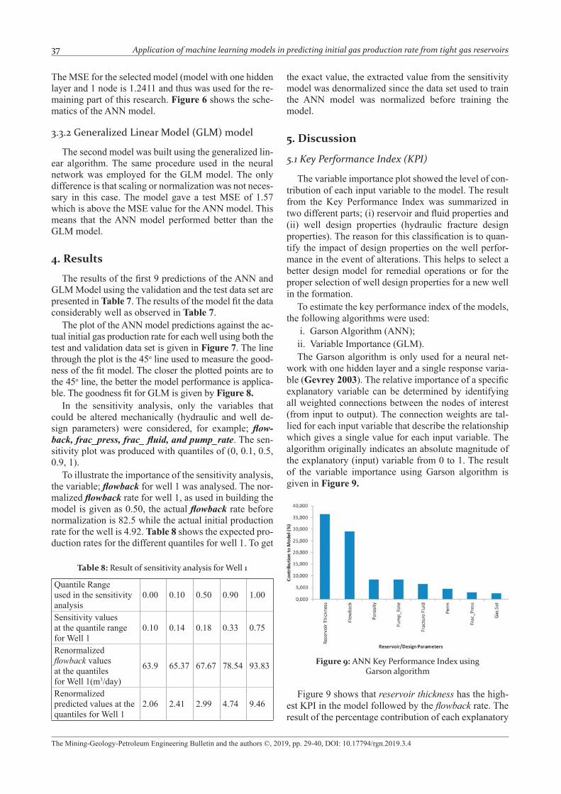
work with one hidden layer and a single response varia-ble (Gevrey 2003). The relative importance of a specifi c explanatory variable can be determined by identifying all weighted connections between the nodes of interest (from input to output). The connection weights are tal-lied for each input variable that describe the relationship which gives a single value for each input variable. The algorithm originally indicates an absolute magnitude of the explanatory (input) variable from 0 to 1. The result of the variable importance using Garson algorithm is given in Figure 9.

Table 8: Result of sensitivity analysis for Well 1

Quantile Range used in the sensitivity analysis

0.00 0.10 0.50 0.90 1.00

Sensitivity values at the quantile range for Well 1

0.10 0.14 0.18 0.33 0.75

Renormalized fl owback values at the quantiles for Well 1(m3/day)

63.9 65.37 67.67 78.54 93.83

Renormalized predicted values at the quantiles for Well 1

2.06 2.41 2.99 4.74 9.46

Figure 9: ANN Key Performance Index using Garson algorithm

Figure 9 shows that reservoir thickness has the high-est KPI in the model followed by the fl owback rate. The result of the percentage contribution of each explanatory



variable is given in the table below. The cumulative sum of the model KPI in the plot equals to 1 or 100%. Table 9 shows the summary of the percentage contribution of the reservoir and fl uid properties and the contribution of the well design parameters to the model.

selected as the best model goes also to suggest that the model with the lowest MSE produces the best KPI. Thus the KPI generated using the Garson algorithm is selected as the best KPI that best explains the data set.

5.2 Look-back analysis

The look-back analysis was conducted to determine the relative performance of each well with regards to the production rate and to determine the expected recovery in the event that some of the production parameters used in the model design were altered. In general, explanatory variables are analysed to determine if the well is under performing, performing as expected or exceeds the ex-pectation rate. It is a general idea that a certain reservoir and fl uid properties do not change with time. For exam-ple, the reservoir thickness remains constant throughout the producing life of a fi eld.

In conducting the look-back analysis, more emphasis was placed on the well design parameters (hydraulic fracturing parameters) of the well that were used to train the model. The aim was to generate a set of random var-iables for the design parameters of the well and keeping the reservoir properties constant, feed the new data set into the model and get a new forecast rate for the each well using the simulated data.

The look-back analysis was based on two categories. For the fi rst category with 5 groups, the results were: ‘excellent = 82 wells (37 %)’, ‘very good = 21 wells (9 %)’, ‘good = 21 wells (9 %)’, ‘average = 28 wells (13 %)’, ‘poor = 72 wells (32 %)’. The results of the second category have 3 groups with results: ‘good = 78 wells (34 %)’, ‘average = 74 wells (32 %)’ and ‘poor = 78 wells (34 %)’.

6. Conclusions

Two Machine Learning models have been presented in this study for the prediction of the initial gas produc-tion rate for tight gas reservoirs using selected reservoir and well parameters. The value that the predictive ana-lytics can add in tight gas production management is of particular importance. The ANN model with one hidden layer was built by cross-validation with a minimum Mean Square Error of 1.24 while the GLM model gave a Mean Square Error of 1.57. This means that the ANN model outperformed the GLM model in forecasting gas production and as such was used for the look-back anal-ysis. The ANN model was also used to rank the KPI of the explanatory variables employed in the predictive model. The KPI shows that the reservoir thickness has the highest contribution to the initial gas production rate followed by the fl owback rate. The reservoir/fl uid prop-erties contribution to initial gas production rate is 53% while the hydraulic fracture parameters contribution to initial gas production rate is 47%. This study concludes

Table 9: Reservoir/well design properties percentage contribution to the data set for ANN

Reservoir properties contribution to the model (%)

Design (hydraulic fracture) parameters contribution to the model (%)

Reservoir Thickness 36.50 Flowback 29.00Porosity 8.50 Pump_Rate 8.50Perm 4.50 Fracture Fluid 6.50Gas.Sat 2.50 Frac_Press 3.00Shale Content 0.10Total 53 47

Table 10: Reservoir/Well design properties percentage contribution to the data Set for GLM

Reservoir properties contribution to the model (%)

Design (hydraulic fracture) parameters contribution to the model (%)

Reservoir Thickness 50.03% Fracture_Fluid 19.00%Perm 3% Flowback 12.00%Gas.Sat 3% Pump_Rate 9.00%Porosity 3% Frac_Press 0.00%Shale Content 1%Total 60% 40%

Figure 10: GLM Key Performance Index

The results of KPI of the variables used in training the GLM model are given in Figure 10. Table 10 shows the percentage contribution of the individual variables grouped under reservoir/fl uid properties and well design properties. The result affi rmed the fact that the initial reservoir thickness contributed the most to the initial gas production. In selecting the best KPI, the MSE rule was used. The idea that the model with the lowest MSE is



that reservoir/well design parameters obtained during geophysical exploration can be used to predict the initial gas production rate of planned new wells from tight gas reservoirs with reasonable accuracy using artifi cial neu-ral networks. Furthermore, the accuracy of prediction of the neural network model depends largely on its archi-tecture (number of hidden layers and number of nodes).

Acknowledgment

This research received fi nancial support (151160638) from the Federal Scholarship Board, Ministry of Educa-tion, Nigeria and the Chinese Government Scholarship Council.

7. References

Abdelkadir B. and Luc. Q. (2014). How to use Big Data Tech-nologies to Optimize Operations in Upstream Petroleum Industry presented at the 21st world petroleum congress in Moscow, Russia 2014. DOI: 10.5585/iji.v1i1.4

Bravo C., Jose. R., Saputtelli. L., Echevarria F. R. (2014). Ap-plying Analytics to production Workfl ows: Transforming Integrated Operations into Intelligent Operations. SPE-167823-MS.. https://doi.org/10.2118/167823-MS

Cipolla C. L. Lolon E.P. Erdle J. C, Rubin B. (2010). Reservoir Modelling of Shale Gas Reservoirs. SPE Res Eval & Eng 13 (4):638-653. SPE-125530. PA.

Cvetković, M., Velić, J., Malvić, T. (2009): Application of neural networks in petroleum reservoir lithology and satu-ration prediction. Geologia Croatica, 62.2, 115–121. doi: 10.4154/gc.2009.10

Dai J., Ni Y, Wu X. (2012). Tight gas in China and its signifi -cance in exploration and exploitation. Journal of Petrole-um Exploration and Development..39, 3, 277–284.

Ding, D.Y, Wu, Y.S, Farah, N., Wang C., Bourbiaux B. (2014). Numerical Simulation of Low Permeability Unconven-tional Gas Reservoirs. SPE-167711-MS. https://doi.org/10.2118/167711-MS

Gevrey, M., Dimopoulos, I., Lek, S. (2003). Review and com-parison of methods to study the contribution of variables in artifi cial neural network models. Ecological Modelling. 160. 249-264.

Gupta.S., Nikolaou.M.,Saputelli.L and Bravo. C. (2016). ESP Health Monitoring KPI: A Real-Time Predictive Analytics Application. SPE-181009-MS. https://doi.org/10.2118/181009-MS

Hastie T., Tibshirani, R,.and Friedman, J. (2001). The Ele-ments of Statistical Learning: Data Mining, Inference, and Predictions. In: Hastie T., Friedman J., Tibshirani R. (eds.): Overview of Supervised Learning. –Springer Publ. Co., 9-40. https://doi.org/10.1007/978-0-387-21606-5

Lantz B. (2015). Machine Learning with R. Second Edition Packt Publishing. Birmingham Mumbai.2015 July.

Malvić, T., Prskalo, S. (2007): Some benefi ts of the neural ap-proach in porosity prediction (Case study from Beničanci fi eld). Nafta, 58/9, 455–467.

Malvić, T., Velić, J., Horváth J., Cvetković, M., (2010). Neural networks in petroleum geology as interpretation tools. Central European Geology, 53.1, 97–115. DOI: 10.1556/CEuGeol.53.2010.1.6

Šapina M. (2016). A comparison of artifi cial neural networks and ordinary kriging depth maps of the lower and upper Pannonian stage border in the Bjelovar Subdepression, Northern Croatia. Rudarsko-geološko-naftni zbornik (The Mining-Geology-Petroleum Engineering Bulletin), 34. 75-86. DOI: 10.17794/rgn.2016.3.6

National Energy Administration (2011) Oil and gas industry standard of the People’s Republic of China: Geological evaluating methods for tight sandstone gas. Beijing: Petro-leum Industry Press. SY/T 6832-2011

Schuetter J., Mishra S., Zhang M. and Lafollette R. (2015). Data Analytics for Production Optimization in Unconven-tional Reservoirs presented at Unconventional Resources Technology Conference, San Antonio, Texas, USA 2015. https://doi.org/10.15530/URTEC-2015-2167005

Tingting L., Lifa Z., Zunsheng J., Yong B., Suli W. (2014). The Ordos Basin: A premier basin for integrating geological CO2 storage with enhanced oil recovery projects in China. ScienceDirect: Energy Procedia. 63. 7772 – 7779.

Trent J. (2016) Analytics Firms Explore Oil and Gas Market. Journal of Petroleum Technology. October 2016. 36-38.

Wei X., Chen H, Zhang D, Dai R, Guo Y, Chen J, Ren J, Liu N, Luo S, Zhao J. (2017). Gas exploration potential of tight carbonate reservoirs: A case study of Ordovician Majiagou Formation in the eastern Yi-Shan slope, Ordos Basin, NW China. Journal of Petroleum Exploration and Develop-ment. 44. 3. 347–357

Zou, C., Z. Zhang, L. Ping, W. Lan, L. Zhong, and L. Liuhong (2010). Shallow-lacustrine sand-rich deltaic depositional cycles and sequence stratigraphy of the Upper Triassic Yanchang Formation, Ordos Basin, China: Basin Re-search, 22, 108–125. https://doi.org/10.1111/j.1365-2117.2009.00450.x

Zhao J., Xu H., Tang D., Mathews J. P., Li S., Tao S. (2016). Coal seam porosity and fracture heterogeneity of macro-lithotypes in the Hancheng Block, eastern margin, Ordos Basin, China. International Journal of Coal Geology. 159, 18-29 https://doi.org/10.1016/j.coal.2016.03.019

Zhou P., Sang H., Jin L., Lee W.J. (2017). Application of Sta-tistical Methods to Predict Production from Liquid Rich Shale Reservoirs presented at Unconventional Resources Technology Conference, Austin, Texas, USA 2017. DOI 10.15530/urtec-2017-2694668

Internet sources:

China National Petroleum Corporation (2008). 19-Ordos Ba-sin [PDF fi le]. Retrieved from http://www.cnpc.com.cn/en/xhtml/pdf/19-Ordos%20Basin.pdf (accessed 18th Feb-ruary, 2019)

United States Environmental Protection Agency. The Process of Unconventional Natural Gas Production.https://www.epa.gov/uog/process-unconventional-natural-gas-produc-tion. (accessed 4th September 2018).



8. Nomenclature

Gas_Sat Gas Saturation (%)Perm Permeability (103milli-darcy)MSE Mean Squared ErrorPump_rate Fracture liquid Pump rate (m3/

min)Flowback Liquid Flowback Rate (%)Frac-press Fracture Pressure need to for

Hydraulic Fracturing (KPa)Porosity Porosity (%)Frac_fl uid Volume of Fracture Fluid (m3)Reservoir_thickness Thickness of a formation where

a well is located (m)Prod_rate Initial Gas production rate of

the wells (m3/day)

SAŽETAK

Primjena strojnoga učenja u predviđanju početne proizvodnje plina iz ležišta male propusnosti

Napredak tehnologije pridobivanja iz ležišta male propusnosti, tj. nekonvencionalnih ležišta, pridonio je znatnoj proiz-vodnji iz takve vrste ležišta ugljikovodika. Broj prikupljenih podataka ogroman je i većina ili svi su u digitalnome obliku. Strojno učenje jedan je od načina kako se takvi podatci mogu analizirati i time povezati niz (zavisnih i nezavisnih) vari-jabli. Predviđanje početne proizvodnje ima važnu ulogu u planiranju i opremanju samih ležišta i polja, a time utječe na odluke o investicijama te izvješća predana regulatornim agencijama. Ovdje je prikazana analiza ležišnih stijena i fl uida na temelju bušotinskih podataka. Načinjen je model odlučivanja kojim je određen početni iznos proizvodnje iz nekon-vencionalnoga ležišta. Uporabljena su dva modela predviđanja razvijena strojnim učenjem – umjetna neuronska mreža (UNM) te poopćeni linearni model (PLM). Izračunan je očekivani iscrpak novih bušotina. Srednja kvadratna pogrješka (SKP) za PLM iznosila je 1,57, a za UNM 1,24. Indeks ključnih svojstava pokazao je kako debljina ležišta ima najveći utjecaj (36,5 %) na početnu proizvodnju plina, a zatim slijedi povratni protok (29 %). Svojstva ležišta i fl uida zajednički sudjeluju u početnoj proizvodnji s 53 %, dok ostalih 47 % otpada na parametre hidrauličnoga frakturiranja.

Ključne riječi:analiza predviđanja, strojno učenje, umjetna neuronska mreža, početna proizvodnja plina, povratna analiza

Authors contribution

Ugwumba Chrisangelo Amaechi (Assistant, MSc) led the research, performe d the Data and Cluster analyis and built the ANN and GLM models used in this work. Princewill Maduabuchi Ikpeka (Lecturer, PhD Candidate) performed the Look-Back analysis and wrote the paper. Ma Xianlin (Professor, PhD) initialized the idea of the research and contri-buted in all the obtained results. Ugwu Johnson (Senior Lecturer, PhD) technically improved the work.

application of machine learning models in predicting

Documents