intelligible models for healthcare: predicting pneumonia...
TRANSCRIPT

Intelligible Models for HealthCare: Predicting PneumoniaRisk and Hospital 30-day Readmission
Rich CaruanaMicrosoft Research
Yin LouLinkedIn Corporation
Johannes GehrkeMicrosoft
Paul KochMicrosoft Research
Marc SturmNewYork-Presbyterian Hospital
Noémie ElhadadColumbia University
ABSTRACTIn machine learning often a tradeoff must be made betweenaccuracy and intelligibility. More accurate models such asboosted trees, random forests, and neural nets usually arenot intelligible, but more intelligible models such as logisticregression, naive-Bayes, and single decision trees often havesignificantly worse accuracy. This tradeoff sometimes limitsthe accuracy of models that can be applied in mission-criticalapplications such as healthcare where being able to under-stand, validate, edit, and trust a learned model is important.We present two case studies where high-performance gener-alized additive models with pairwise interactions (GA2Ms)are applied to real healthcare problems yielding intelligiblemodels with state-of-the-art accuracy. In the pneumoniarisk prediction case study, the intelligible model uncoverssurprising patterns in the data that previously had pre-vented complex learned models from being fielded in thisdomain, but because it is intelligible and modular allowsthese patterns to be recognized and removed. In the 30-day hospital readmission case study, we show that the samemethods scale to large datasets containing hundreds of thou-sands of patients and thousands of attributes while remain-ing intelligible and providing accuracy comparable to thebest (unintelligible) machine learning methods.
Categories and Subject DescriptorsI.2.6 [Computing Methodologies]: Learning—Induction
Keywordsintelligibility; classification; interaction detection; additivemodels; logistic regression; healthcare; risk prediction
1. MOTIVATIONIn the mid 90’s, a large multi-institutional project was
funded by Cost-Effective HealthCare (CEHC) to evaluate
Permission to make digital or hard copies of all or part of this work for personal orclassroom use is granted without fee provided that copies are not made or distributedfor profit or commercial advantage and that copies bear this notice and the full citationon the first page. Copyrights for components of this work owned by others than theauthor(s) must be honored. Abstracting with credit is permitted. To copy otherwise, orrepublish, to post on servers or to redistribute to lists, requires prior specific permissionand/or a fee. Request permissions from [email protected]’15, August 10-13, 2015, Sydney, NSW, Australia.Copyright is held by the owner/author(s). Publication rights licensed to ACM.ACM 978-1-4503-3664-2/15/08 ...$15.00.DOI: http://dx.doi.org/10.1145/2783258.2788613 .
the application of machine learning to important problems inhealthcare such as predicting pneumonia risk. In the study,the goal was to predict the probability of death (POD) forpatients with pneumonia so that high-risk patients could beadmitted to the hospital while low-risk patients were treatedas outpatients. In the study [3, 2], the most accurate mod-els that could be trained were multitask neural nets.1 Onone dataset the neural nets outperformed traditional meth-ods such as logistic regression by wide margin (the neuralnet had AUC=0.86 compared to 0.77 for logistic regression),and on the other dataset used in this paper outperformedlogistic regression by about 0.02 (see Table 2). Althoughthe neural nets were the most accurate models, after carefulconsideration they were considered too risky for use on realpatients and logistic resgression was used instead. Why?
One of the methods being evaluated was rule-based learn-ing [1]. Although models based on rules were not as accurateas the neural net models, they were intelligible, i.e., inter-pretable by humans. On one of the pneumonia datasets,the rule-based system learned the rule “HasAsthama(x) ⇒LowerRisk(x)”, i.e., that patients with pneumonia who havea history of asthma have lower risk of dying from pneumo-nia than the general population. Needless to say, this ruleis counterintuitive. But it reflected a true pattern in thetraining data: patients with a history of asthma who pre-sented with pneumonia usually were admitted not only tothe hospital but directly to the ICU (Intensive Care Unit).The good news is that the aggressive care received by asth-matic pneumonia patients was so effective that it loweredtheir risk of dying from pneumonia compared to the generalpopulation. The bad news is that because the prognosis forthese patients is better than average, models trained on thedata incorrectly learn that asthma lowers risk, when in factasthmatics have much higher risk (if not hospitalized).
One of the goals of the study was to perform a clinical trialto determine if machine learning could be used to predictrisk prior to hospitalization so that a more informed decisionabout hospitalization could to be made. The ultimate goalwas to reduce healthcare cost by reducing hospital admis-sions, while maintaining (or even improving) outcomes bymore accurately identifying patients that need hospitaliza-tion. As the most accurate models, neural nets were a strongcandidate for clinical trial. Deploying neural net models thatcould not be understood, however, was deemed too risky —
1SVMs and boosted trees were not in common use yet, andRandom Forests had not yet been invented.
1721

if the rule-based system had learned that asthma lowers risk,certainly the neural nets had learned it, too. The rule-basedsystem was intelligible and modular, making it easy to recog-nize and remove dangerous rules like the asthma rule. Whilethere are methods for repairing the neural nets so they donot incorrectly predict that asthmatics are at lower risk andthus less likely to need hospitalization, e.g., re-train withoutasthmatics in the population, remove the asthma feature,modify the targets for asthmatics to “1” in the data to re-flect the care they received (unfortunately confounding carewith death), the decision was made to not use the neural netsnot because the asthma problem could not be solved, but be-cause the lack of intelligibility made it difficult to know whatother problems might also need fixing. Because the neuralnets were more accurate than the rules, it was possible thatthe neural nets had learned other patterns that could putsome kinds of patients at risk if used in a clinical trial. Forexample, perhaps pregnant women with pneumonia also re-ceive aggressive treatment that lowers their risk comparedto the general population. The neural net might learn thatpregnancy lowers risk, and thus recommend not admittingpregnant women, thus putting them at increased risk. In aneffort to “do no harm”, the decision was made to go forwardonly with models that were intelligible such as logistic regres-sion, even if they had lower AUC than other unintelligiblemodels. The logistic regression model also learned that hav-ing asthma lowered risk, but this could easily be correctedby changing the weight on the asthma feature from negativeto positive (or to zero).
Jumping two decades forward to the present, we nowhave a number of new learning methods that are very ac-curate, but unfortunately also relatively unintelligible suchas boosted trees, random forests, bagged trees, kernelized-SVMs, neural nets, deep neural nets, and ensembles of thesemethods. Applying any of these methods to mission-criticalproblems such as healthcare remains problematic, in partbecause usually it is not ethical to modify (or randomize)the care delivered to patients to collect data sets that willnot suffer from the kinds of bias described above. Learningmust be done with the data that is available, not the dataone would want. But it is critical that models trained onreal-world data be validated prior to use lest some patientsbe put at risk, which makes using the most accurate learningmethods challenging.
In this paper we describe the application of a learningmethod based on high-performance generalized additive mod-els [5, 6] to the pneumonia problem described above, and toa modern, much larger problem predicting 30-day hospitalreadmission. On both of these problems our GA2M modelsyield state-of-the-art accuracy while remaining intelligible,modular, and editable. We believe this class of models repre-sents a significant step forward in training models with highaccuracy that are also intelligible. The main contributions ofthis paper are that it: shows that GA2Ms yield competitiveaccuracy on real problems; demonstrates that the learnedmodels are intelligible; demonstrates that the predictionsmade by the model for individual cases (patients) also areintelligible, and demonstrates how, because the models aremodular, they can be edited by experts.
The remainder of the paper is organized as follows. Sec-tion 2 provides a brief introduction to GAM and GA2M.Sections 3 and 4 present our case studies of training intelli-gible GA2M model on the pneumonia and the 30-day read-
mission data, respectively. Section 5 discusses a wide rangeof issues that arise when learning with intelligible modelsand our general lessons for the research community.
2. INTELLIGIBLE MODELSLet D = {(xi, yi)}N1 denote a training dataset of size N ,
where xi = (xi1, ..., xip) is a feature vector with p featuresand yi is the target (response). We use xj to denote the jthvariable in the feature space.
Generalized additive models (GAMs) are the gold stan-dard for intelligibility when low-dimensional terms are con-sidered [4, 5, 6]. Standard GAMs have the form
g(E[y]) = β0 +∑
fj(xj), (1)
where g is the link function and for each term fj , E[fj ] = 0.Generalized linear models (GLMs), such as logistic regres-sion, are a special form of GAMs where each fj is restrictedto be linear. Since the contribution of a single feature to thefinal prediction can be easily understood by examining fj ,such models are considered intelligible.
To improve accuracy, pairwise interactions can be addedto standard GAMs, leading to a model called GA2Ms [6]:
g(E[y]) = β0 +∑j
fj(xj) +∑i6=j
fij(xi, xj). (2)
Note that pairwise interactions are intelligible because theycan be visualized as a heat map. GA2M builds the bestGAM first and then detects and ranks all possible pairs ofinteractions in the residuals. The top k pairs are then in-cluded in the model (k is determined by cross-validation).
There are various methods to train GAMs and GA2Ms.Each component can be represented using splines, leading toan optimization problem which balances the smoothness ofsplines and empirical error [7]. Other representations includeregression trees on a single or a pair of features. Empiricalstudy showed gradient boosting with bagging of shallow re-gression trees yields as components very good accuracy [5].Interested readers are referred to [5, 6] for details.2
3. CASE STUDY: PNEUMONIA RISKIn this case study we use one of the pneumonia datasets
discussed earlier in the motivation [3]. This dataset has14,199 pneumonia patients. To facilitate comparison withprior work, we use the same train and test set folds from theearlier study: the train set contains 9847 patients and thetest set has 4352 patients (a 70:30 train:test split). Thereare 46 features describing each patient. These range fromhistory features such as age and gender, to simple measure-ments taken at a routine physical such as heart rate, bloodpressure, and respiration rate, to lab tests such as WhiteBlood Cell count (WBC) and Blood Urea Nitrogen (BUN),to features read from a chest x-ray such as lung collapse orpleural effusion. See Table 1 for a complete list.
As discussed earlier, the goal is to predict probability ofdeath (POD) so that patients at high risk can be admit-ted to the hospital, while patients at low risk are treated asoutpatients.3 10.86% of the patients in the dataset (1542 pa-tients) died from pneumonia. The GAM/GA2M models are2Code is available at https://github.com/yinlou/mltk.3Hospitals are dangerous places, particularly for patientswith impaired immune systems. Treating low-risk patientsas outpatients not only saves money, but is actually safer.
1722

Patient-history findingschronic lung disease - age Cre-admission to hospital - gender -admitted through ER - diabetes mellitus -admitted from nursing home - asthma -congestive heart failure - cancer -ischemic heart disease - number of diseases Ccerebrovascular disease - history of seizures -chronic liver disease - renal failure -history of chest pain -
Physical examination findingsdiastolic blood pressure C wheezing -gastrointestinal bleeding - stridor -respiration rate C heart murmur -altered mental status - temperature Cheart rate C
Laboratory findingsliver function tests - BUN level Cglucose level C creatinine level Cpotassium level C albumin level Chematocrit C WBC count Cpercentage bands C pH CpO2 C pCO2 Csodium level C
Chest X-ray findingspositive chest x-ray - lung infiltrate -pleural effusion - pneumothorax -cavitation/empyema - chest mass -lobe or lung collapse -
Table 1: Pneumonia attributes, grouped bytype. Continuous features that will be shaped byGAM/GA2M models are marked with a “C”.
trained on this data using 100 rounds of bagging. Bagging isdone to reduce overfitting, and to provide pseudo-confidenceintervals for the graphs in the intelligible model.
The AUC area for different models trained on this data areshown in Table 2. On this dataset logistic regression achievesAUC = 0.843, Random Forests achieves 0.846, LogitBoost0.849, GAM 0.854, and GA2M is best with AUC = 0.857.4
The difference in AUC between the methods is not huge (lessthan 0.02), but it is reassuring to see the GAM/GA2M meth-ods achieve the best accuracy on this problem. The im-portant question is if the GAM/GA2M models are able toachieve this accuracy while remaining intelligible?
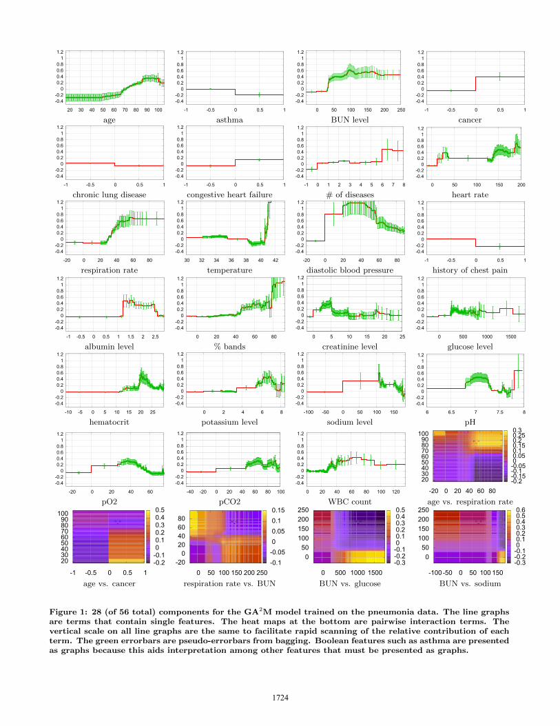
Figure 1 shows 28 of the 56 terms in the GA2M modelfor pneumonia. Unfortunately, the compact representationnecessary for the paper reduces intelligibility. For smallmodels like this with fewer than 100 terms we would pre-fer to present all terms, possibly sorted by their importanceto the model. In the actual deployment, for each term wewould also show a histogram of data density for differentvalues of the feature, descriptive statistics about the fea-ture, several different measures of term importance in themodel, and links to online resources that provide informa-tion about the term, e.g., links to a hospital database, orWikipedia or WebMD pages that describe features, how theyare measured, what the normal ranges are, and what abnor-mal values indicate. Because of space limitations we havesuppressed all of this auxiliary information (including someaxis labels!) and just present shape plots for some of themore interesting terms. Presenting the terms in multicol-umn format without the auxiliary information further hin-ders intelligibility — the models are more readable when
4The GA2M model uses 10 of the 46∗45/2 = 1035 possiblepairwise interaction terms (k chosen by cross-validation).
Model Pneumonia Readmission
Logistic Regression 0.8432 0.7523
GAM 0.8542 0.7795GA2M 0.8576 0.7833
Random Forests 0.8460 0.7671LogitBoost 0.8493 0.7835
Table 2: AUC for different learning methods on thepneumonia and 30-day readmission tasks.
presented in sorted order as a scrollable list of graphs plusauxiliary information.
The 1st term in the model is for age. Age (in years) on thex-axis ranges from 18-106 years old (the pneumonia datasetcontains only adults). The vertical axis is the risk scorepredicted by the model for patients as a function of age. Therisk score for this term varies from -0.25 for patients with ageless than 50, to a high of about 0.35 for patients age 85 andabove. The green errorbars are pseudo-errorbars of the riskscore predicted for each age: each errorbar is ±1 standarddeviation of the variation in the risk score measured by 100rounds of bagging. We use ±1 standard deviation insteadof the standard error of the mean because it is well knownthat bagging underestimates the variance of predictions fromcomplex models. We believe it is safer to be conservativethan to present unrealistically narrow confidence intervals.(See the top of Figure 3(a) for an enlarged version of thisgraph, and the discussion in Section 5.5 for more detailedanalysis of the age feature.)
The 2nd term in the model, asthma, is the one that causedtrouble in the CEHC study in the mid-90’s and preventedclinical trials with the very accurate neural net model. TheGA2M model has found the same pattern discovered backthen: that having asthma lowers the risk of dying from pneu-monia. As with the logistic regression and rule-based mod-els trained then, but unlike with the neural net models, thisterm is easy to recognize and fix in the GA2M model. Wecan “repair” the model by eliminating this term (effectivelysetting the weight on this graph to zero), or by using hu-man expertise to redraw the graph so that the risk scorefor asthma=1 is positive, not negative. Because asthma isboolean, it is not necessary to use a graph, and we couldpresent a weight and offset (RiskScore = w*hasAsthma +b) instead. We prefer to use graphs for boolean terms likeasthma for three reasons: 1) it is necessary to show graphsfor features with multiple or continuous values such as ageas well as for interactions between features, and it is awk-ward for the user to jump from terms presented as graphs toterms presented as equations; 2) we find graphs provide anintuitive display of risk where up implies higher risk, downimplies lower risk, and the magnitude of the change in risk iscaptured by the distance moved; and 3) some users are notas comfortable with numbers as they are with graphs, andit is important that the model is intelligible to real users,whatever their background.
The 3rd term in the model is BUN (Blood Urea Nitro-gen) level. Most patients have BUN=0 because, as in manymedical datasets, if the variable is not measured or assumednormal it is coded as 0. The model says risk is reducedfor patients where BUN was not measured, suggesting thatthis test typically is not ordered for patients who appearto be healthy. BUN levels below 30 appear to be low risk,
1723
-0.4-0.2
0 0.2 0.4 0.6 0.8
1 1.2
20 30 40 50 60 70 80 90 100
-0.4-0.2
0 0.2 0.4 0.6 0.8
1 1.2
-1 -0.5 0 0.5 1
-0.4-0.2
0 0.2 0.4 0.6 0.8
1 1.2
0 50 100 150 200 250
-0.4-0.2
0 0.2 0.4 0.6 0.8
1 1.2
-1 -0.5 0 0.5 1
age asthma BUN level cancer
-0.4-0.2
0 0.2 0.4 0.6 0.8
1 1.2
-1 -0.5 0 0.5 1
-0.4-0.2
0 0.2 0.4 0.6 0.8
1 1.2
-1 -0.5 0 0.5 1
-0.4-0.2
0 0.2 0.4 0.6 0.8
1 1.2
-1 0 1 2 3 4 5 6 7 8
-0.4-0.2
0 0.2 0.4 0.6 0.8
1 1.2
0 50 100 150 200
chronic lung disease congestive heart failure # of diseases heart rate
-0.4-0.2
0 0.2 0.4 0.6 0.8
1 1.2
-20 0 20 40 60 80
-0.4-0.2
0 0.2 0.4 0.6 0.8
1 1.2
30 32 34 36 38 40 42
-0.4-0.2
0 0.2 0.4 0.6 0.8
1 1.2
-20 0 20 40 60 80
-0.4-0.2
0 0.2 0.4 0.6 0.8
1 1.2
-1 -0.5 0 0.5 1
respiration rate temperature diastolic blood pressure history of chest pain
-0.4-0.2
0 0.2 0.4 0.6 0.8
1 1.2
-1 -0.5 0 0.5 1 1.5 2 2.5
-0.4-0.2
0 0.2 0.4 0.6 0.8
1 1.2
0 20 40 60 80
-0.4-0.2
0 0.2 0.4 0.6 0.8
1 1.2
0 5 10 15 20 25
-0.4-0.2
0 0.2 0.4 0.6 0.8
1 1.2
0 500 1000 1500
albumin level % bands creatinine level glucose level
-0.4-0.2
0 0.2 0.4 0.6 0.8
1 1.2
-10 -5 0 5 10 15 20 25
-0.4-0.2
0 0.2 0.4 0.6 0.8
1 1.2
0 2 4 6 8
-0.4-0.2
0 0.2 0.4 0.6 0.8
1 1.2
-100 -50 0 50 100 150
-0.4-0.2
0 0.2 0.4 0.6 0.8
1 1.2
6 6.5 7 7.5 8
hematocrit potassium level sodium level pH
-0.4-0.2
0 0.2 0.4 0.6 0.8
1 1.2
-20 0 20 40 60
-0.4-0.2
0 0.2 0.4 0.6 0.8
1 1.2
-40 -20 0 20 40 60 80 100
-0.4-0.2
0 0.2 0.4 0.6 0.8
1 1.2
0 20 40 60 80 100 120
"-"
-20 0 20 40 60 80
20 30 40 50 60 70 80 90
100
-0.2-0.15-0.1-0.05 0 0.05 0.1 0.15 0.2 0.25 0.3
pO2 pCO2 WBC count age vs. respiration rate
"-"
-1 -0.5 0 0.5 1
20 30 40 50 60 70 80 90
100
-0.2-0.1 0 0.1 0.2 0.3 0.4 0.5
"-"
0 50 100 150 200 250-20
0 20 40 60 80
-0.1-0.05 0 0.05 0.1 0.15
"-"
0 500 1000 1500
0 50
100 150 200 250
-0.3-0.2-0.1 0 0.1 0.2 0.3 0.4 0.5
"-"
-100 -50 0 50 100 150
0 50
100 150 200 250
-0.3-0.2-0.1 0 0.1 0.2 0.3 0.4 0.5 0.6
age vs. cancer respiration rate vs. BUN BUN vs. glucose BUN vs. sodium
Figure 1: 28 (of 56 total) components for the GA2M model trained on the pneumonia data. The line graphsare terms that contain single features. The heat maps at the bottom are pairwise interaction terms. Thevertical scale on all line graphs are the same to facilitate rapid scanning of the relative contribution of eachterm. The green errorbars are pseudo-errorbars from bagging. Boolean features such as asthma are presentedas graphs because this aids interpretation among other features that must be presented as graphs.
1724

while levels from 50-200 indicate higher risk. This is con-sistent with medical knowledge which suggests that normal,healthy BUN is 10-20, and that elevated levels above 30 mayindicate kidney damage, congestive heart failure, or bleedingin the gastrintestinal tract.
The cancer term in the model is clear: having cancer sig-nificantly increases the risk of dying from pneumonia, prob-ably because it explains why the patient has pneumonia (ei-ther from lung cancer, from immuno suppressive drugs usedto treat cancer, or from hospitalization associated with can-cer) and/or because it explains the stage of cancer (terminalstages of cancer frequently lead to failing health and beingbed-ridden, both of which can lead to pneumonia).
The next term in the model, chronic lung disease, and thehistory of chest pain term that occurs later, are interestingbecause the model suggests that chronic lung disease and ahistory of chest pain both decrease POD. We suspect thatthis may be a similar problem as asthma: patients withlung disease and chest pain may receive care earlier, andmay receive more aggressive care. If further investigationsuggests this to be the case, both terms would be removedfrom the model, or edited, similar to the asthma term.
The # of diseases (# of comorbid conditions) is a generalmeasure of illness. The graph suggests that having no dis-eases other than pneumonia lowers risk, that risk increasesslowly as the number of comorbid conditions increases from1-3, then is flat or decreases until it rises dramatically above6, but the errorbars are large enough to be consistent withrisk being somewhat flat for 3-8 comorbidities.
Heart rate is an unusual looking graph. 91% patientshave rate=0, indicating it was not measured or assumednormal. Risk is high for very low heart rates (10-30), andfor very high rates (125-200), but the model does not ap-pear to discriminate between patients with heart rates 40-120. On further inspection, there are no patients with heartrate recorded between 40-120! Apparently all patients inthis range were considered “normal” and coded as 0. (Nor-mal heart rate in adults is about 60-100, 40-60 for athletes,and somewhat higher than 100 for patients with “WhiteCoat” Syndrome). The unusual shape of the graph for heartrate has lead us to discover a surprising aspect of the data,though it is not clear what risk we would want to model topredict for rates between 40-120 where there is no data?
The respiration rate term is very clear: rate=0 (missing)or 20-28 is low risk, and risk rises rapidly as breathing rateclimbs from 28-60. Normal respiration rate for adults is16-20. In the body temperature term, temps from 36◦C-40◦C are low risk (normal is 37◦C), risk is somewhat elevatedat low body temps (32◦C-36◦C), and greatly elevated fortemps above 40.5◦C (fever this high often is a sign of seriousinfection). Having a fever above 41.5◦C increases the riskscore by a full point or more.5 Diastolic blood pressure alsocan dramatically increase risk: low diastolic in the range 20-50 (normal is 60-80) increase risk as much as a full point. %bands is also a strong term (bands in a blood test are a signof bacterial infection—bacterial pneumonia is more deadlythan viral pneumonia): bands above 40% indicate elevatedrisk, with bands above 80% indicating very elevated risk.
Before leaving pneumonia, let us examine one of the inter-action terms. In the age vs. cancer term, we see that risk ishighest for the youngest patients (probably cancers acquired
5An increase in risk of 1 point more than doubles the oddsof dying. See Section 5.1.
in childhood but not cured when the patient reaches age 18),and declines for patients who acquire cancer later in life, butfor patients without cancer risk rises as expected with age.This is a classic interaction effect that likely results from thedifference between childhood and adult cancers.
Space prevents us from discussing each term individually,or from discussing terms in great detail. See Section 5.5 for adeeper dive on the age term. To summarize this section, theGA2M model discovered the same asthma pattern that cre-ated problems in the CEHC study, provides a simple mech-anism to correct this problem, and uncovered other similarproblems (chronic lung disease and history of chest pain)that were not recognized in the CEHC study but which war-rant further investigation and probably repair. As hoped,the GA2M model is accurate, intelligible, and repairable.
4. CASE STUDY: 30-DAY READMISSIONIn this section we apply GA2M to a modern and much
larger dataset for 30-day hospital readmission. The datacomes from a collaboration with a large hospital. Thereare 195,901 patients in the train set (2011-2012), 100,823patients in the test set (2013), and 3,956 features for eachpatient. Features include lab test results, summaries of doc-tor notes, and details of previous hospitalizations. In thisproblem, the goal is to predict which patients are likely tobe readmitted to the hospital within 30 days after being re-leased from the hospital. All patients in this dataset havealready been hospitalized at least once, and the goal is topredict if they will need to return to the hospital unusuallyquickly (within 30 days). Hospitals with abnormally high30-day readmission rates are penalized financially becausea high rate suggests the hospital did not provide adequatecare on the earlier admission, or may have released the pa-tient prematurely, or did not provide adequate instructionsto the patient when they were released, or did not performadequate follow-up after release. In the data 8.91% of pa-tients are readmitted within 30 days. For this problem weuse 10 iterations of bagging. Training the 10 models takes2-3 days on a small cluster of 10 general purpose computers.Table 2 shows the AUC for different models on this data.
In Section 3 we examined the GA2M model for the pneu-monia problem. Unfortunately, the readmission dataset con-tains almost 100 times as many features. Instead of tryingto examine the full model, we instead examine the predic-tions made by the model for three patients. Two of thesepatients have very high predicted probability of readmission(p=0.9326 and p=0.9264), and one of the patients has a typ-ical readmission probability (p=0.0873). This allows us todemonstrate that the models are intelligible not only takenas a whole, but that the predictions GA2M models make forindividual patients also are intelligible.
In Figure 2, each of the three columns is a patient, andeach row is a term in the model. Terms are sorted for eachpatient (in each column) by the risk they contribute to thatpatient for 30-day readmission. Space limits us to showingthe top 6 terms for each patient that contributed most torisk. Patient #1 has a very high probability of readmissionwithin 30 days: p=0.9326. The four terms that contributemost to their high probability of readmission are: their totalnumber of visits to the hospital is 40, they have been an in-patient in the hospital 19 times in the last 12 months, theyhave been in the hospital 10 times in the last 6 months, and4 times in the last 3 months. This is not unusual: the most
1725

Patient 1: 0.9326 Patient 2: 0.9264 Patient 3: 0.0873
-0.2
0
0.2
0.4
0.6
0 10 20 30 40 50
0.3140
-0.2
0
0.2
0.4
0.6
0 20 40 60 80 100 120 140 160
0.3334
-0.2
0
0.2
0.4
0.6
0 5 10 15 20 25 30 35
0.0704
# inpatient visits ever prednisone preparations endometrial carcinoma
-0.2
0
0.2
0.4
0.6
0 5 10 15 20 25
0.3017
-0.2
0
0.2
0.4
0.6
0 500 1000 1500 2000 2500
0.3144
-0.2
0
0.2
0.4
0.6
0 5 10 15 20 25 30 35 40
0.0301
# inpatient visits last 12 months etoposide preparation Malignant adenomatous neoplasm
-0.2
0
0.2
0.4
0.6
0 2 4 6 8 10 12 14 16
0.2780
-0.2
0
0.2
0.4
0.6
0 2000 4000 6000 8000 10000
0.2536
-0.2
0
0.2
0.4
0.6
0 20 40 60 80 100 120 140
0.0251
# inpatient visits last 6 months mesna prepartions clonazepam preparations
-0.2
0
0.2
0.4
0.6
0 2 4 6 8 10
0.2144
-0.2
0
0.2
0.4
0.6
0 50 100 150 200 250 300 350 400
0.2451
-0.2
0
0.2
0.4
0.6
-20 0 20 40 60 80
0.0250
# inpatient visits last 3 months doxorubicin preparations whole blood hematocrit tests max
-0.2
0
0.2
0.4
0.6
0 500 1000 1500 2000
0.1990
-0.2
0
0.2
0.4
0.6
0 20 40 60 80 100
0.2102
-0.2
0
0.2
0.4
0.6
0 5 10 15 20
0.0239
amoxicillin preparations dexamethasone preparations Intraductal carcinoma of breast
-0.2
0
0.2
0.4
0.6
0 50 100 150 200 250 300 350 400 450
0.1867
-0.2
0
0.2
0.4
0.6
0 5 10 15 20
0.1830
-0.2
0
0.2
0.4
0.6
0 50 100 150 200 250 300 350 400 450
0.0220
verapamil preparations ondansetron hydrochloride preparations # outpatient visits ever
Figure 2: Top 6 terms (of 4456) in the GA2M for three patients. The patients on the left have high risk ofreadmission. The patient on the right has moderate risk. Terms are sorted by their contribution to risk.Blue lines highlight feature values and corresponding risk scores. Six terms cannot tell the full story for thesepatients, but even these few terms provide insight into the patients and their risk of readmission.
1726

predictive terms in the 30-day readmission model measurethe number of visits patients have made in the last 12 month,6 months, and 3 months to the ER, as an outpatient, and asan inpatient. As we see with this patient, a large number ofrecent inpatient visits (admissions) is associated with a highprobability of readmission.6 The next two terms suggestwhy patient #1 may have been in the hospital often: thispatient has received large doses of amoxicillin (an antibioticused to treat infections like strep and pneumonia) and ver-apamil (a treatment for hypertension and angina), i.e., theyhave an ongoing infection that may not be responding toantibiotics, and also probably have heart disease. The mainreason this patient is predicted to be likely to return is be-cause they have been in the hospital often in the last year,but the first few terms in the model also give us a hint ofthe medical conditions that put them at elevated risk.
The terms that are most important for patient #2 (alsohigh risk: p=0.9364) are different from the terms that wereimportant for patient #1. The most important 6 termsare preparations that the patient received during their lastvisit: prednisone is a corticosteroid used as an imummo-suppressant, etoposide in an anticancer drug, mesna is acancer chemotherapy drug, doxorubicin is a treatment forblood and skin cancers, dexamethosone is another immuno-suppressant steroid, and ondansetron is a drug used to treatnausea from chemotherapy. Patient #2 has received dosesof each of these preparations that suggest cancer may not beresponding well to treatment and that they are receiving ag-gressive chemotherapy. The contribution to risk from these6 terms alone is greater than +1.5, i.e., these 6 terms alonetriple the odds of their being readmitted within 30-days.
Patient #3 has moderate risk: p=0.0873 (baseline rateis 8.91%). This 6 terms that increase this patient’s read-mission risk the most are: 1) the patient has endrometrialcarcinoma (a cancer common in post-menopausal womenthat often can be treated effectively by hysterectomy with-out radiation- or chemo-therapy); 2) a benign abdominaltumor (malignant adenomatous neplasm =3); 3) a relaxanttypically prescribed to calm patients or reduce spasms; 4) afairly typical (i.e. low risk) hematocrit test result; 5) a pre-cancerous non-invasive lesion in the breast; and 6) a smallnumber of outpatient visits suggesting they have been re-ceiving treatment as an outpatient without needing to behospitalized (the inpatient and ER risk factors for this pa-tient are all low). Patient #3 is a typical patient as far as 30-day readmission is considered. They are post-menopausal,have cancers that respond well to treatment if caught early,the treatments themselves are relatively low-risk, and theyhave not needed unusual medications or to be hospitalizedoften in the last year.
The patients above provide a small glimpse of what theGA2M model learned from a 200,000 patient train set with4,000 features: we have only been able to examine threepatients, and have only looked at the top 6 terms for eachof these patients. To a medical expert, the sorted terms
6A large number of visits to the ER also is associated withincreased chance of readmission, but outpatient visits aremore interesting: a small number of recent outpatient visitsincreases risk of readmission, but a very large number ofoutpatient visits (100-200 in the last year) indicates lowerrisk of readmission because the patient is receiving primarycare as an outpatient—many of these patients are dialysispatients who visit the hospital 1-2 times per week.
RiskScore Probability RiskScore Probability
-5.0 0.0067 +5.0 0.9933-4.0 0.0180 +4.0 0.9820-3.0 0.0474 +3.0 0.9526-2.0 0.1192 +2.0 0.8808-1.0 0.2689 +1.0 0.73110.0 0.5000
Table 3: Risk scores (log odds) and the correspond-ing probabilities.
for each patient present a comprehensive picture of the riskfactors that contribute to the probability of readmission pre-dicted for a patient. The model is not causal — it does notsay that because the patient has X, they received treatmentsA, B, and C, and we can see from the amount of A, B, andC they received that they are not responding well. Instead,it learns that high doses of A, B, and C are associated withhigh risk or readmission, and it is up to the human expertsto infer the underlying causal reasons for the feature valuesand the risk they predict. Nevertheless, compared to an un-intelligible model such as an ensemble of 1000 boosted treesor a complex neural net, the model is fairly transparent, andthe predictions it makes can be fully “understood”, both atthe per-patient level, and at the macro-model level.
5. DISCUSSION
5.1 How To Interpret Risk ScoresEach term in the intelligible model returns a risk score
(log odds) that is added to the patient’s aggregate predictedrisk. Terms with risk scores above zero increase risk; termswith scores below zero decrease risk. The term risk scoresare added to a baseline risk, and the sum converted to aprobability. Both penumonia and 30-day readmission havebaseline rates near 0.1, which corresponds to TotalRiskScore= -2.197. So patients with aggregate risk scores above -2.2have higher than average risk, and patients with total riskscores below -2.2 have lower than average risk scores. A pa-tient with TotalRiskScore = 0 (including the baseline offset)has quite high risk: p = 1/(1+exp(−1∗TotalRiskSccore) =1/(1 + exp(0)) = 0.5. Table 3 shows a sample of total riskscores and the corresponding probabilities.
5.2 ModularityIn the intelligible models discussed in this paper, the av-
erage risk score for each graph (i.e., each term: each featureor pair of features) averaged across the training set is setto zero by subtracting the mean score. A single bias termis then added to the model so that the average predictedprobability across all patients equals the observed baselinerate. This is done to make models identifiable and modular.Because of this property, each graph can be removed fromthe model (zeroed out) without introducing bias to the pre-dictions. If all terms were removed from the model, the onlyremaining term would be the bias term, and the probabilitypredicted for all patients would be the observed baseline ratein the training set. Adding terms (graphs) to the model in-creases the model’s discriminativeness without altering theprior. This is important because it increases modularity andmakes it easier to interpret the contribution of each term:
1727

negative scores decrease risk, and positive scores increaserisk compared to the baseline risk.
5.3 Sorting Terms by ImportanceIf a model contains a modest number of terms (e.g., less
than 50), it is best to show terms in the model to expertsin the order they are most familiar with. Because expertsare often used to seeing features in logical groupings, inter-pretation is aided by preserving these groupings when themodel is presented. However, when the number of termsgrows large, it becomes infeasible for experts to examine allterms carefully. Term importance often follows a power-lawdistribution, with a few terms being very important, a mod-est number of terms being somewhat important, and manyterms being of little importance. When this is the case, in-telligibility can be improved by sorting terms by a measureof importance such as the drop in AUC when the term isremoved, or the skill of the term measured in isolation, orthe maximum contribution (positive or negative) that theterm can make for any patient. No one measure is corrector best, and we find that a sort that reflects a combinationof these metrics seems to work well.
It is much easier to sort terms by importance when makingprediction for a single patient: because each term yields asingle risk score for each patient at the point where thatpatient’s feature value lies on the term graph, it is possible tosort terms by how much they increase or decrease risk for thepatient. This provides a well-defined ordering of the termsfor a patient from terms that increase risk most to terms thatdecrease risk most. Often this ordering quickly identifiesthe key patient characteristics that best explain the model’sprediction, and which help experts quickly understand thepatient’s condition. This is the method we used to describethe predictions made by the 30-day readmission model —although that model contains more than 4000 terms, thenumber of terms that are relevant for each patient are, inpractice, often quite small (e.g., less than 100).
5.4 Feature Shaping vs. Expert DiscretizationSignificant effort was made in the CEHC pneumonia study
to train accurate models with logistic regression and othermethods that could not handle continuous attributes. Med-ical experts carefully discretized each continuous attributeinto clinically meaningful ranges used to define boolean vari-ables. For example, the intervals for age were 18-39, 40-54,55-63, 64-68, 69-72, 73-75, 76-79, 80-83, 84-88, and 89+. Weused these expert-defined intervals for the logistic regressionmodel reported in Table 2. We also trained a GA2M modelwith these discretized features, and observed a drop in AUCof about 0.01 on the test set compared to the GA2M trainedwith the continuous features, suggesting that the GA2M modelgains some of its accuracy by shaping continuous featuresmore accurately than expert discretization.
5.5 Deep Dive: Risk as a Function of AgeIn this section we drill down on how the feature “Age”
is shaped by the pneumonia and 30-day readmission mod-els. Age is present in both data sets and measured in years.But the relevance of age to the two prediction tasks is verydifferent. In pneumonia, age is a critical factor that can ex-plain why a patient has acquired pneumonia, and what the
-0.4
-0.2
0
0.2
0.4
0.6
20 30 40 50 60 70 80 90 100
Pne
umon
ia R
isk
Sco
re
age
0
0.03
20 30 40 50 60 70 80 90 100
Den
sity
(a) Pneumonia
-0.06-0.04-0.02
0 0.02 0.04 0.06
0 20 40 60 80 100Re-
Adm
issi
on R
isk
Sco
re
age
0
0.15
0 20 40 60 80 100
Den
sity
(b) 30-day Readmission
-0.1
-0.05
0
0.05
0.1
0 0.5 1 1.5 2Re-
Adm
issi
on R
isk
Sco
re
age(c) 30-day Readmission (zoomed in)
Figure 3: Risk as a function of Age for the Pneumo-nia and 30-day Readmission problems.
outcome is likely to be.7 In 30-day all-cause readmission,
7Pneumonia is sometimes called “The Old Man’s BestFriend”, not because pneumonia is good for elderly patients,but because it often results in rapid death for patients thatotherwise could linger for months or years before their pri-mary illness causes death.
1728

20 40 60 80 100
−4−2
02
4
age
Pne
umon
ia R
isk
Sco
re
6.0 6.5 7.0 7.5 8.0
−4−2
02
4
pH
Pne
umon
ia R
isk
Sco
re
30 32 34 36 38 40 42
−4−2
02
4
temperature
Pne
umon
ia R
isk
Sco
re
Figure 4: Selected splines in pneumonia dataset.
however, age is just one of thousands of factors that affecta patient’s health and course of illness. Moreover, becausethe prediction task is hospital readmission, not probabilityof death, age represents a weaker, more generic characteriza-tion of patient health and their likeliness to need additionalhospitalization within 30 days. If the patient is elderly, butjust had a successful hip replacement or kidney stone re-moved, they are not likely to need to return to the hospitalwithin 30 days for this condition. Similarly, an elderly pa-tient who was admitted to the hospital because of pneumo-nia, but who is now being released because they respondedto treatment, is unlikely to need further care for pneumoniawithin 30 days if they take proper medications. All-causereadmission is very different from probability of death for aspecific condition such as pneumonia.
Figure 3(a) shows the risk profile for age in the pneumo-nia model, and the distribution of age in the pneumoniadata. The majority of pneumonia patients are age 60-90.Qualitatively, the risk of dying from pneumonia is low andconstant from age 18-50, rises slowly from age 50-66, thenrises quickly from age 66-90, and then levels off at very highrisk above age 90. The low-risk region to the left of age 50 isremarkably flat, suggesting that the underlying trees rarelyif ever found it useful to split this region into subregions.Note that the risk score for this region is -0.27, suggestingthat being young significantly reduces the risk of dying frompneumonia. But risk slowly increases as age increases above50, though the contribution to risk does not become positiveuntil about 70 years. Beyond 70 years old, the contributionto risk rises rapidly from 0.0 at 70 to +0.20 at age 82 and+0.35 at age 86. According to the model, the increase inrisk of going from 70 to 86 is larger than the decrease is riskof going from 70 down to 50 or less.
Beyond the risk vs. age profile described above, there areintriguing details in the graph. 1) There is a small jumpin risk at age 67, and again at age 86. The error bars arereasonably tight around age 65-70, suggesting that the jumpin risk at 67 may be real. One possible explanation for thisis that in a dataset from the 90’s, many patients would haveretired at around age 65, and that this may yield differ-ences in activity levels, health insurance, and willingness toget access healthcare early enough to improve outcomes —pneumonia responds well to treatment with antibiotics, butcan be life threatening if not treated. The 2nd jump in riskaround age 86 is harder to explain. It may be that practi-tioners, either consciously or subconsciously, treat patients
older than 85 differently, and that this ultimately increasestheir POD. Or the jump at 86 may be an artifact of themodel — the error bars at age 86 and above are larger. Oneapproach to investigating this issue further would be to trainon another sample sample of data (or on different subsam-ples) to see if the rise at age 86 persists.8 2) There is anapparent drop in risk above age 100. We suspect that thisdrop probably is not real and may be due to mild overfit-ting — there are very few patients age 95 and older, and theerror bars from age 90 to 106 are large and consistent withrisk being constant in this region.9 3) Surprisingly, there isno evidence that risk, although very high, increases aboveage 85. Either medical treatments are equally effective forpatients older than 85, or other medical conditions are morelikely to be responsible for death at this age than pneumo-nia, or risk does increase above 85 and the model has failedto learn it.
Figure 3(b) shows the age term and density for 30-dayreadmission. One of the key differences between the pneu-monia and 30-day readmission datasets is that pneumoniadataset contains only adult patients age 18 and older, butthe readmission dataset contains patients of all age, includ-ing newborn infants. The importance of age to 30-day read-mission is very different. Age has little effect on readmissionbetween age 2 and 50, risk slowly increases from age 50 to 80,and then increases a little more above age 80. The largestincrease in score is +0.03 at age 90 and above. There aremany reasons why age is less important for readmission thanfor pneumonia: most patients independent of age would notbe released if the hospital thought they were likely to needto be readmitted in less than a month, in this dataset thereare thousands of other more specific variables that can bet-ter explain variance in the risk of readmission (the modelis more illness specific) than age, and some patients whoare very elderly will die at home (either unexpectedly or bychoice) and thus will not be readmitted.
8It is only because the model is so intelligible that we areable to recognize and question such fine detail in the risk vs.age profile. We assume that similar jumps in predicted riskoccur in other accurate models such as boosted trees as well,but because those models are less intelligible the jumps arenot recognized or investigated.9Or it might be due to successful agers, a rare but geneti-cally identifiable class of people with traits that better en-able them to survive into old age
1729

An interesting feature of the model for 30-day readmis-sion is highlighted in Figure 3(c) where the x axis has beenexpanded to show age 0-2. In this dataset newborn infantsare born into the hospital, and thus will be treated as read-mitted if they need to be hospitalized within 30 days aftergoing home. In part because newborns would not be re-leased if they were at risk, the risk score for newborns age0-2 months is -0.04—this is a larger negative risk score thanthe increase in risk for elderly patients. This suggests thatmost newborns tend to be healthy when they are releasedfrom the hospital and are less likely to need to be readmittedwithin 30 days. But this reduction in risk from being new-born diminishes after 2-3 months, and the model suggeststhat infants age 3-15 months have slightly higher positiverisk of being readmitted to the hospital. Thus infants age 3-15 months have higher risk of readmission than infants thatare younger or older, and it is not until age 45 that the riskof readmission rises to this level again.
5.6 Shaping with SplinesGeneralized additive models are often fit with splines [7].
Splines allow GAMs to be trained with careful control overregularization and provide more principled error bars. Un-fortunately, the spline methods tend to over regularize, yieldless accuracy than GA2M models, and yield risk profiles thatsometimes miss detail discovered by GA2M models. Figure 4shows three terms from a spline GAM model trained on thepneumonia data. The 1st term is age, the 2nd is pH, and the3rd is temperature. Although the splines capture the basictrends (e.g., risk increases with age, pH risk is least around7.6, and fever risk rises above 40◦C), the splines miss detaillearned by GA2M. For example, the GA2M model for ageis much more nuanced, and the spline model may not prop-erly model temperature in the normal range 36◦C-38◦C. Thespline GAM model has accuracy closer to logistic regressionthan GA2M, so the extra detail learned by GA2M increasesaccuracy and probably reflects genuine structure.
5.7 Correlation Does Not Imply CausationBecause the models in this paper are intelligible, it is
tempting to interpret them causally. Although the modelsaccurately explain the predictions they make, they are stillbased on correlation. If features were added to or subtractedand the model retrained, the graphs for some terms that hadremained in the model would change because of correlationwith the features added or subtracted. Although details ofsome of the shape plots are suggestive (e.g., does pneumoniarisk truly jump as age increases above 65, and again above85?), it is not (yet) clear if some details like this are due to a)overfitting; b) correlation with other variables; c) interactionwith other variables; d) correlation or interaction with un-measured variables; or e) due to true underlying phenomenasuch as retirement and change in insurance provider.
Perhaps the strongest statement we can make right now isthat the models are intelligible enough to provide a windowinto the data and prediction problem that is missing withmany other learning methods, and that this window allowsquestions to be raised that will require investigation andfurther data analysis to answer. In future versions of thesemodels we hope to automate some of these analyses so thatit is clearer what features in the intelligible model are “real”or due to random factors such as overfitting and spurious
correlation. Adding causal analysis to the models would betremendously useful, but is, of course, difficult.
6. CONCLUSIONSWe present two case studies on real medical data where
GA2Ms achieve state-of-the-art accuracy while remaining in-telligible. On the pneumonia case study the GA2M modellearns patterns that previously prevented complex machinelearning models from being deployed, but because GA2M isintelligible and modular it is possible to edit the model to re-duce deployment risk. On the larger, more complex 30-dayhospital readmission task the GA2M model achieves excel-lent accuracy while yielding a manageable, surprisingly intel-ligible model despite incorporating over 4000 terms. Usingthis problem we demonstrate how GA2Ms can be used toexplain the predictions the model makes for individual pa-tients in a concise way that places focus on the most impor-tant/relevant terms for each patient. We believe GA2Ms rep-resent a significant step forward in the tradeoff betweenmodel accuracy and intelligibility that should make it easierto deploy high-accuracy learned models in applications suchas healthcare where model verification and debuggability areas important as accuracy.
Acknowledgements. We thank Michael Fine, MD, Uni-versity of Pittsburgh School of Medicine, and Greg Cooper,MD, PhD, University of Pittburgh for help with the Pneu-monia data and model. We thank Eric Horvitz, MD, PhD,Microsoft Research Redmond for help with the 30-day hos-pital readmission data and model. The 30-day hospital read-mission experiment was reviewed and approved by the insti-tutional review board at Columbia University Medical Cen-ter.
7. REFERENCES[1] R. Ambrosino, B. Buchanan, G. Cooper, and M. Fine.
The use of misclassification costs to learn rule-baseddecision support models for cost-effective hospitaladmission strategies. In Proceedings of the AnnualSymp. on Comp. Application in Medical Care, 1995.
[2] G. Cooper, V. Abraham, C. Aliferis, J. Aronis,B. Buchanan, R. Caruana, M. Fine, J. Janosky,G. Livingston, T. Mitchell, S. Montik, and P. Spirtes.Predicting dire outcomes of patients with communityacquired pneumonia. Journal of BiomedicalInformatics, 38(5):347–366, 2005.
[3] G. Cooper, C. Aliferis, R. Ambrosino, J. Aronis,B. Buchanan, R. Caruana, M. Fine, C. Glymour,G. Gordon, B. Hanusa, J. Janosky, C. Meek,T. Mitchell, T. Richardson, and P. Spirtes. Anevaluation of machine-learning methods for predictingpneumonia mortality. Artificial Intelligence inMedicine, 9(2):107–138, 1997.
[4] T. Hastie and R. Tibshirani. Generalized additivemodels. Chapman & Hall/CRC, 1990.
[5] Y. Lou, R. Caruana, and J. Gehrke. Intelligible modelsfor classification and regression. In KDD, 2012.
[6] Y. Lou, R. Caruana, J. Gehrke, and G. Hooker.Accurate intelligible models with pairwise interactions.In KDD, 2013.
[7] S. Wood. Generalized additive models: an introductionwith R. CRC Press, 2006.
1730