application of computational symmetry to … of computational symmetry to histology images . ......
TRANSCRIPT
Application of Computational Symmetry to Histology Images
Brian Canada and Yanxi Liu [email protected], [email protected]
Tech. report CMU-RI-TR-08-08, Robotics Institute, Carnegie Mellon University, January, 2008.
Abstract—The larval zebrafish is an ideal organism for studying mutant phenotypes (observable traits) because of its small size and rapid, ex vivo development. Histology is one highly sensitive means for detecting and scoring zebrafish mutants, and while “high-throughput” methods have been developed for preparing digital “virtual slides” of zebrafish larval histology, problems of subjectivity and labor bottlenecks associated with scoring these virtual slides impede large-scale histological analysis from being widely adopted in zebrafish laboratories. Here, we demonstrate that novel computer vision techniques derived from and inspired by the current state-of-the-art algorithms for computational symmetry detection have the potential to improve the efficiency and accuracy of the histology image preparation and classification workflow, thereby bringing the overall process closer to being more fully automated and truly “high-throughput.”
I. INTRODUCTION AND BACKGROUND
A. Use of the zebrafish for high-throughput phenotyping and problems with the current paradigm
The zebrafish has been shown to be an excellent model organism for vertebrate
development and human disease, largely because its transparent, readily accessible embryo develops outside the mother’s body, and most organ systems are well differentiated by 7 days post-fertilization [1], allowing mutant phenotypes to be readily identified in a relatively short amount of time. Many phenotype assignments in zebrafish are based on assessments of gross morphology. While this practice is invaluable, gross morphological analysis cannot provide precise characterization of phenotypes. For example, several zebrafish mutants analyzed using gross morphology have relatively nonspecific eye phenotypes (e.g., “small” or “reduced” eyes). Histology—the microscopic study of biological tissues—is much more sensitive than gross analysis in that mutant phenotypes can be explored at much finer levels of detail. In the case of eye phenotypes, for instance, histology can identify individual cell death and morphological disruptions in specific retinal cell layers, which is not possible using conventional gross analysis techniques.
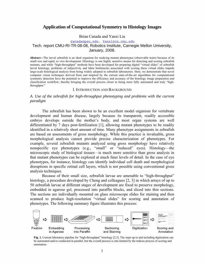
Because of their small size, zebrafish larvae are amenable to “high-throughput” histology, a procedure developed by Cheng and colleagues [2, 3] in which arrays of up to 50 zebrafish larvae at different stages of development are fixed to preserve morphology, embedded in agarose gel, processed into paraffin blocks, and sliced into thin sections. The sections are individually mounted on glass microscope slides for staining and then scanned to produce high-resolution “virtual slides” for scoring and annotation of phenotypes. The following summary figure illustrates this process:
Fig. 1. Current laboratory pipeline for “high-throughput” histology [2,3]. The steps up to and including digitization can
be automated and/or conducted in parallel, but the overall process is rate-limited by the tedious process of scoring and annotation.
1
The phrase “high-throughput,” as used in this context, does not currently apply to all steps in the pipeline, however. While fixation, embedding, sectioning, staining, and digitization of an entire array of larvae may be conducted in parallel (in the sense that in each of these steps, multiple larvae are being processed together), the process of scoring each image is rate limiting. Comprehensive annotation of the phenotype requires scoring several levels (planar sections) of each larva. While this process is manageable when manually annotating a small number of larvae, the task becomes increasingly impractical as the number of larvae rises.
Even if a laboratory were to hire a technician to work exclusively on manually scoring images, the process would still be quite slow and tedious. For example, in a large-scale mutagenesis screen involving hundreds of genes, thousands of images will be generated. These images may or may not exhibit a mutant phenotype, but the technician does not know in advance which images fall into either category, and must spend an inordinate amount of time sifting out images of “normal” histology. Complicating the matter is the problem of subjectivity in the process of scoring and annotating the images. While largely reliable and useful clinically, the qualitative aspects of current histological assessments result in intra- and inter-observer variability [4]. This variability can be due to differences in training, ability, timing, and experience.
As a result of the impracticalities of histological analysis (despite its higher detection sensitivity), many zebrafish laboratories do not utilize this method for phenotyping because of the effort, expense, and expertise required to collect, score, and annotate the resulting images. Therefore, in order to maximize the effectiveness of histological studies as applied to animal model systems, it became critical to us that some form of automatic, quantitative method be developed for the analysis of zebrafish histology images. In an effort to address this need, we recently developed a prototype system for the automated segmentation, feature extraction, and classification of zebrafish histology images [5]. Ultimately, these methods will form the core of SHIRAZ (System of Histological Image Retrieval and Annotation for Zoopathology), a novel computational framework for the automated, ontology-based annotation and retrieval of histological images for quantitative, “high-throughput” phenotyping in animal model systems. This framework is ultimately intended for use with histology images for a variety of animal models, but owing to our experience in zebrafish genetic studies and histological analysis, the zebrafish serves as a compelling pilot model for prototype development. Currently, SHIRAZ is capable of segmenting zebrafish larval eye and gut (intestine) histology images and classifying them according to varying degrees of abnormality, with preliminary accuracies ranging from 55% to 90% depending on the type of tissue being analyzed as well as the number of possible categories used in automatic classification (i.e., binary vs. multi-class). While these results demonstrate the potential of the SHIRAZ system for scoring images objectively, quantitatively, and automatically, the classification accuracy can certainly be improved, perhaps by improving the quality of the segmentation or by increasing the number and variety of extracted features. Moreover, the overall efficiency of the high-throughput histology workflow is still limited by the fact that the pre-processing steps required to prepare images for input into SHIRAZ are carried out manually. These steps, illustrated in the figure below, include the extraction of individual specimens from virtual slides, the
2
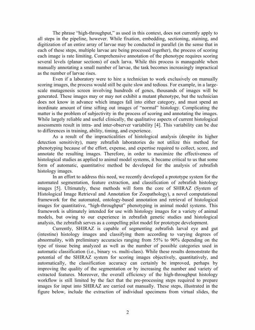
identification of the category of the specimen (normal, mutant, or indeterminate) by correlating the position of the specimen on the virtual slide with its corresponding entry in the laboratory’s embedding record for that particular zebrafish mutant, as well as the extraction of specific organ images from the specimen’s whole-larva image.
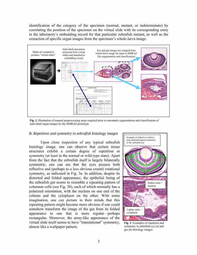
B. Repetition and symmetry in zebrafish histology images Upon close inspection of any typical zebrafish histology image, one can observe that certain tissue structures exhibit a certain degree of repetition or symmetry (at least in the normal or wild-type state). Apart from the fact that the zebrafish itself is largely bilaterally symmetric, one can see that the eyes possess both reflective and (perhaps to a less obvious extent) rotational symmetry, as indicated in Fig. 3a. In addition, despite its distorted and folded appearance, the epithelial lining of the zebrafish gut seems to resemble a repeating pattern of columnar cells (see Fig. 3b), each of which normally has a polarized orientation, with the nucleus on one end of the column and the cytoplasm on the other. With some imagination, one can picture in their minds that this repeating pattern might become more obvious if one could somehow transform the image of the gut from its folded appearance to one that is more regular—perhaps rectangular. Moreover, the array-like appearance of the virtual slide itself seems to have “translational” symmetry, almost like a wallpaper pattern,
Darker stain = nucleus
Lighter stain = cytoplasm
Example of reflective (yellow) and rotational (green) symmetry in the zebrafish eye
Individual specimens extracted from virtual slides and matched to
embedding record
Eye and gut images are cropped from whole-larva image for input to SHIRAZ
(for segmentation and classification)
Slides are scanned to produce “virtual slides”
Fig. 2. Illustration of manual preprocessing steps required prior to automatic segmentation and classification of individual organ images by the SHIRAZ prototype.
Fig. 3. Examples of repetition and symmetry in zebrafish eye (a) and gut (b) histology images.
3

at least in the sense that the specimens (or “tiles”) in the array are all oriented in the same direction, are equidistant from one to the next, and more or less look similar (see Fig. 4), though this similarity can vary depending on the depth and orientation of the specimen when it is originally embedded in the tissue block; indeed, the embedding process is far from perfect, since the yaw, roll, and pitch angles of many specimens show departures from zero, sometimes significantly. Fig. 4. Example virtual slide of a zebrafish larval array
Conceivably, one could exploit these features of repetition and symmetry for the purpose of improving the quality of the feature extraction process as well as the efficiency of the overall high-throughput histology workflow. For example, a cursory assessment of some sample images seems to indicate that the degree of symmetry or repetition is less apparent for the mutant eye and gut images (see Fig. 5 for example comparisons). Furthermore, one could take advantage of the grid or lattice-like layout of the zebrafish larval array for extracting individual specimen images and matching them up with their positions in the embedding record. Finally, if one could reliably produce three-dimensional reconstructions of “stacks” of zebrafish images from the same specimen, then the reconstructed specimen could be re-oriented so that its yaw, roll, and pitch angles are as close to zero as possible. This re-oriented model could then be virtually “re-sliced” so that each section exhibits bilateral symmetry as closely as is possible (we say “possible” because the zebrafish normally does exhibit left-right asymmetry in some organ systems, particularly in the digestive system).
Normal eye Mutant eye Normal gut Mutant gut
Fig. 5. Example comparisons of normal and mutant zebrafish eye and gut histology. C. Evaluation of current symmetry detection algorithms A number of computational symmetry detection algorithms have appeared in recent literature, and some of these may have potential applicability to identifying repetition and symmetry in 2D and 3D zebrafish images. Here, we review a selection of state-of-the-art algorithms for detection of reflection symmetry, rotational symmetry, and translational symmetry, as well as methods for re-orientation of 3D images (specifically MRI brain images) to achieve the best possible reflection symmetry about the so-called mid-saggital plane. In addition, we have evaluated each method’s ability to analyze
4

zebrafish histology images, even though none of these was developed specifically for such an application. Two of these methods were evaluated for detecting reflection symmetry in zebrafish histology images. The first of these, by Liu et al. [6], was developed for the purpose of detecting implied dihedral and/or frieze symmetry group structure based on the relative orientation of all potential detected reflection symmetry axes in an image. (A dihedral symmetry group is made up of pairwise-associated rotational and reflective symmetries; for example, a regular polygon has n sides, so it has n rotational symmetries and n reflective symmetries, for a total of 2n symmetries. Frieze symmetry groups, in contrast, are used to describe repetitive patterns in only one linear direction.) Potential reflection axes are identified within an exhaustive search for pairwise matches in 2D polar-coordinate space, with the coordinates (r, θ) defined with respect to the center of the image. Parallel axes imply frieze group detection, while intersecting axes imply dihedral group detection.
The second method, by Loy and Eklundh [7], is based on Lowe’s SIFT (Scale-Invariant Feature Transform) algorithm for object recognition in images [8] but extended to identify both bilateral and rotational symmetry. SIFT is a fairly robust approach to identifying objects in a scene when the object has been subjected to affine transformations (translation, rotation, scaling, etc.) and/or small geometric distortions with respect to the target object in the scene, and it even works when the target object in the scene is occluded by other objects. Briefly, SIFT works by first identifying points of extrema (keypoints) in so-called “scale space” and then computing histograms that represent the magnitude and canonical orientation of the gradients around each of these keypoints. The histogram information for each keypoint is captured in a 128-element feature vector. In Loy/Eklundh’s method, the detection of bilateral symmetry relies on flipping the keypoints about those axes corresponding to the dominant canonical orientation (when considering all keypoints in the image simultaneously). Detection of rotational symmetry, on the other hand, simply involves looking for pairs of matching keypoint feature vectors that yield canonical orientations that are not parallel to each other. In other words, if the vectors are not parallel, then they must intersect at some point, and the point of intersection is taken to be a putative center of rotation.
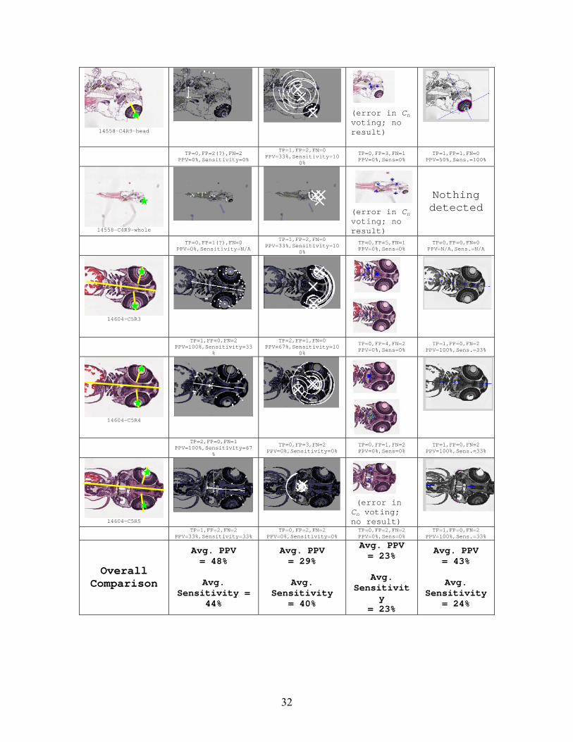
We tested the Liu and Loy/Eklundh methods on a set of eye, head, and whole-larva images of zebrafish histology, since all such images should exhibit bilateral symmetry to some extent, at least for normal (wild-type) specimens. Each method was evaluated using metrics of positive predictive value (PPV) and sensitivity. Here, PPV is defined as the number of true reflection symmetry axes detected divided by the total of all reflection symmetry axes detected, whether true or false (in other words, the PPV tells you what percentage of the algorithm’s guesses were correct.) Sensitivity is defined as the number of true axes detected divided by the sum of the number of true positives and false negatives (in other words, the sensitivity tells you what percentage of the actual ground truth axes were detected by the algorithm). Based on our analysis using 15 test images, the Loy/Eklundh algorithm proved to be superior, with a PPV of 48% and sensitivity of 44% in comparison to Liu’s method, which yielded a PPV of 43% and a sensitivity of 24%. In some cases, the Liu method detected no symmetry axes whatsoever, and therefore the PPV could not be calculated for those instances and was left out of the overall average (see Appendix A for detailed results).
5

For detection of rotational symmetry, two additional methods were evaluated along with the Loy/Eklundh algorithm described above. Prasad and Davis [9] developed a rotational symmetry detection algorithm based on the use of a so-called “gradient vector flow” (GVF) field, which itself is a characterization of an image’s gradient magnitude field and is primarily used to indicate the diffusion path followed by a “snake” that deforms itself around an object until it converges to detect the edges of the object. In order to detect n-fold rotational symmetry about some object in the image, the GVFs detected along the edge points must be rotations of each other by the angle 360°/n (or 2π/n radians), the colors must be similar, and the points must lie approximately along the edges of a polygon with n sides.
In the third method, Lee et al. [Lee, Collins and Liu 2008] employ a markedly different approach to rotational symmetry detection. Instead of identifying candidate keypoints (as in the Loy/Eklundh algorithm) or edge points (as in the Prasad algorithm) from the original image, Lee et al’s method converts the image to a different coordinate system—almost like converting between polar and Cartesian coordinates. The idea here is that by “re-mapping” the image to a new coordinate system, any rotational symmetry in the original image (if it exists) would be transformed into translational symmetry in one direction; in other words, the expanded image would yield a frieze pattern (consequently, Lee et al’s algorithm has been dubbed the “frieze expansion” method). The advantage here is that the algorithm will still work (in theory, at least) even if there are no detected SIFT keypoints, which is a requirement of the Loy/Eklundh method. Therefore, images that have relatively low contrast (and therefore have almost no gradients to be identified using SIFT) can still be used, so long as the contrast is not so low that a candidate center of rotation cannot be identified.
Two different evaluations were conducted for the rotational symmetry detection methods. The first evaluation, involving only the Loy/Eklundh and Prasad/Davis algorithms, was conducted using the same set of 15 images that was used in the reflection symmetry detection evaluation described above. The same two metrics are used (PPV and sensitivity), but instead of detecting axes of reflective symmetry, we are detecting centers of rotational symmetry. In this first evaluation, the Loy/Eklundh algorithm (PPV=29%, sensitivity=40%) outperformed the Prasad/Davis method (PPV=23%, sensitivity=23%). Not only was the Loy/Eklundh method more accurate, but its execution time was at least an order of magnitude faster.
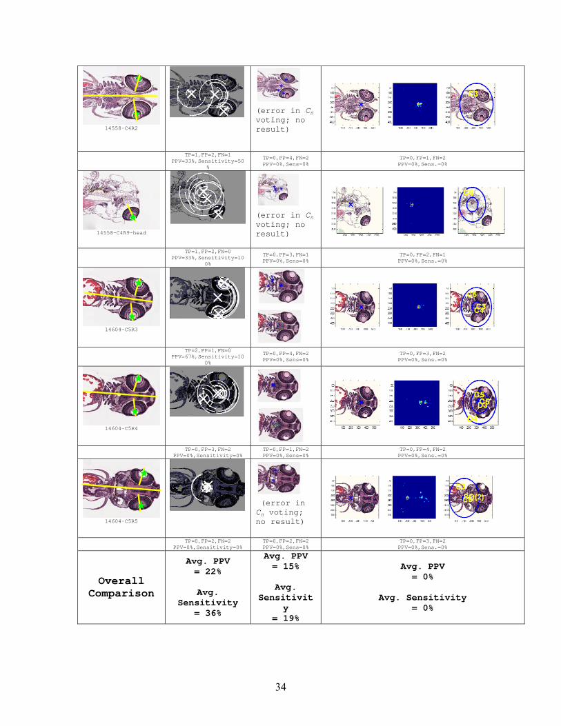
In the second evaluation, all three of the rotational symmetry detection methods were evaluated together, using 9 images of zebrafish larval head histology. Once again, Loy/Eklundh proved to be superior, with an average PPV of 22% and sensitivity of 36% as compared to Prasad/Davis, with a PPV of 15% and a sensitivity of 19%, to identify any true centers of rotation in the zebrafish eye and head images (Appendices A and B for detailed evaluation results). Despite the low success rate of Lee’s frieze-expansion method in detecting the centers of rotational symmetry in the lens of the zebrafish eye (in the context of a whole-head image), it was recognized that the idea behind Lee et al’s algorithm is inspiring and useful for analyzing zebrafish gut images, which do not have “rotational symmetry” per se, but do appear to exhibit some semblance of a repeating pattern of columnar cells as one progresses around the folds of epithelial lining, as was shown previously. To explore the possibility of detecting this type of repeating pattern, we initially used the “frieze
6

expansion” code from Lee et al’s algorithm to transform selected zebrafish gut images from polar to rectangular coordinates. As the figure on the following page indicates, the transformation produces an image in which the epithelial lining is still distorted and folded, but is generally horizontal in appearance. A short procedure was written to extract the lining, one column of pixels at a time, and “normalize” the heights of the extracted columns to produce a “frieze-like expansion” of the epithelial lining. Following this, we performed a Discrete Fourier Transform (DFT)-based autocorrelation (see METHODS section for details) on the image to produce a plot and a “score” that would indicate if there were any repeating patterns in the rectangular image. This procedure was tested on two images—one of abnormal histology, and one of normal (wild-type) histology. As the preliminary results indicate (see Fig. 6), the scaled DFT score for the abnormal gut image was much lower than that of the normal gut image. This led us to the hypothesis that the DFT score of the transformed gut image might be useful for discriminating between normal and abnormal classes of gut images.
Fig. 6a. Example of “frieze expansion” for normal (wild-type) gut histology image
Original gut image
Transformation to rectangular coordinates
(*Note: this and the result below were outputs of the Polar Coordinates filter in Adobe Photoshop CS3, but Lee’s MATLAB-based algorithm
produces a functionally identical result)
Extraction of gut lining followed by normalization of column heights
DFT-based autocorrelation plot
(here, the average DFT “score” is about 140)
Fig. 6b. Example of “frieze expansion” for abnormal gut histology image (continues on next page)
Original gut image
Transformation to rectangular coordinates
7

Example of “frieze expansion” for abnormal gut histology image (cont’d from previous page)
Extraction of gut lining followed by normalization of column heights
DFT-based autocorrelation plot
(here, the average DFT “score” is about 30-40) There were three fundamental problems with using Lee et al’s code to perform the
initial coordinate system transformation, however; first, if the “center of rotation” (about which the transformation would take place) was not contained within the lumen (interior) of the gut, then the transformation could produce an image far too distorted to accurately represent the true “repeating” appearance of the cells contained within lining of the gut (Fig. 7a). Secondly, if the lining itself is significantly folded—that is, there are significantly large villi (fingerlike projections) protruding into the lumen—then there is also a risk of the expanded image being too distorted or discontinuous, even if the center of rotation is fully contained within the lumen (as in Fig. 7b). We concluded that the concept of performing a frieze-like expansion of the gut image was attractive, but we would need to develop and implement an entirely new algorithm to produce a result in which the cells of the lining can be transformed to rectangular coordinates with minimal distortion. Fig. 7a. Example of coordinate transformation of significantly folded tissue, with center of rotation (marked by yellow cross) not contained within the lumen boundary)
x
Fig. 7b. Example of coordinate transformation of significantly folded tissue, with center of rotation (marked by yellow cross) contained within the lumen boundary
x
D. Evaluation of symmetry features for zebrafish histology image classification
8

Because the Loy/Eklundh method had the strongest performance—relatively speaking—for detecting both reflection and rotation symmetry in zebrafish images, it was logical to see if the symmetry features extracted from such images could be used to discriminate between two different classes of images. In the first of three tests, 18 normal (wild-type) zebrafish eye images and 28 abnormal (mutant) zebrafish eye images (all of variable age between 3 and 7 days post-fertilization) were used in a test to discriminate between normal and abnormal zebrafish eye histology. In a second test, this time for discriminating between normal and abnormal gut histology, 33 normal zebrafish gut images and 43 abnormal zebrafish gut images were used. In the third test, we used all 46 eye images and all 76 gut images to train a classifier to discriminate between eye images and gut images, regardless of whether the histology was normal or abnormal.
For reflection symmetry, Loy’s method outputs the number of symmetric features (presumably the number of SIFT keypoint pairs that are symmetric), the number of symmetry axes detected, and the symmetry strengths for each detected symmetry axis. Obviously the number of symmetry axes detected will vary from image to image, and so as a result the number of output scalars (i.e., symmetry strengths) will correspondingly vary. For the purposes of training a classification model, the number of features must be the same for all images. To accomplish this while preserving as much of the original symmetry feature information as possible, we chose to extract the following feature vector for each image:
1. Number of symmetric keypoint pairs 2. Number of symmetry axes detected 3. Maximum detected symmetry strength 4. Minimum detected symmetry strength 5. Mean detected symmetry strength 6. Standard deviation of symmetry strengths
Because symmetries may resolve differently at different image scales, these six features were extracted twice, at scales of 50% and 25%. (The original images are 512 x 512 pixels, but at 100% scale, the speed of the algorithm is compromised, and so smaller scales were chosen for this analysis.)
For rotational symmetry, the Loy/Eklundh method not only outputs the number of symmetric features and the symmetry strength for each of the (at most) three strongest symmetry rotation centers detected, but also the order of rotational symmetry for each of these rotation centers. Since the number of reported centers of rotational symmetry can vary from zero to three, we have condensed this information into a seven-feature vector, similar to that extracted for reflection symmetry as described earlier:
1. Number of symmetric keypoint matches (about a center of rotation) 2. Maximum detected symmetry strength 3. Minimum detected symmetry strength 4. Mean detected symmetry strength 5. Standard deviation of symmetry strengths 6. Maximum rotation order detected 7. Minimum rotation order detected
9
As with the reflection symmetry features, this vector is extracted at both 50% and 25% of the original image scale. All told, 26 features were extracted for each image. Classification was performed using the CART (Classification and Regression Trees) algorithm [10] using ten-fold cross-validation, meaning that rather than having separate training and testing data sets, we train the model on 90% of the data and test it using 10% of the data (randomly selected) that was previously set aside. The process is repeated ten times, with the final error rate being reported as an average of the error rates of the ten individual classification tests. The CART algorithm works by finding a hierarchy of features that yield the best discrimination among the desired set of classes. At the “root node” of the tree, which represents the full data set, the best degree of discrimination (or “best split”) is computed for all features. Once a best split has been chosen for the root node, the data is partitioned into two “child” or “leaf” nodes. This process is repeated until a pre-chosen stopping criterion is reached, such as when the data has been partitioned enough so that all leaf nodes contain, at most, a specified number of samples. After the tree is constructed, it may be found that “pruning” the tree back to a smaller number of terminal nodes may improve the overall classification accuracy.
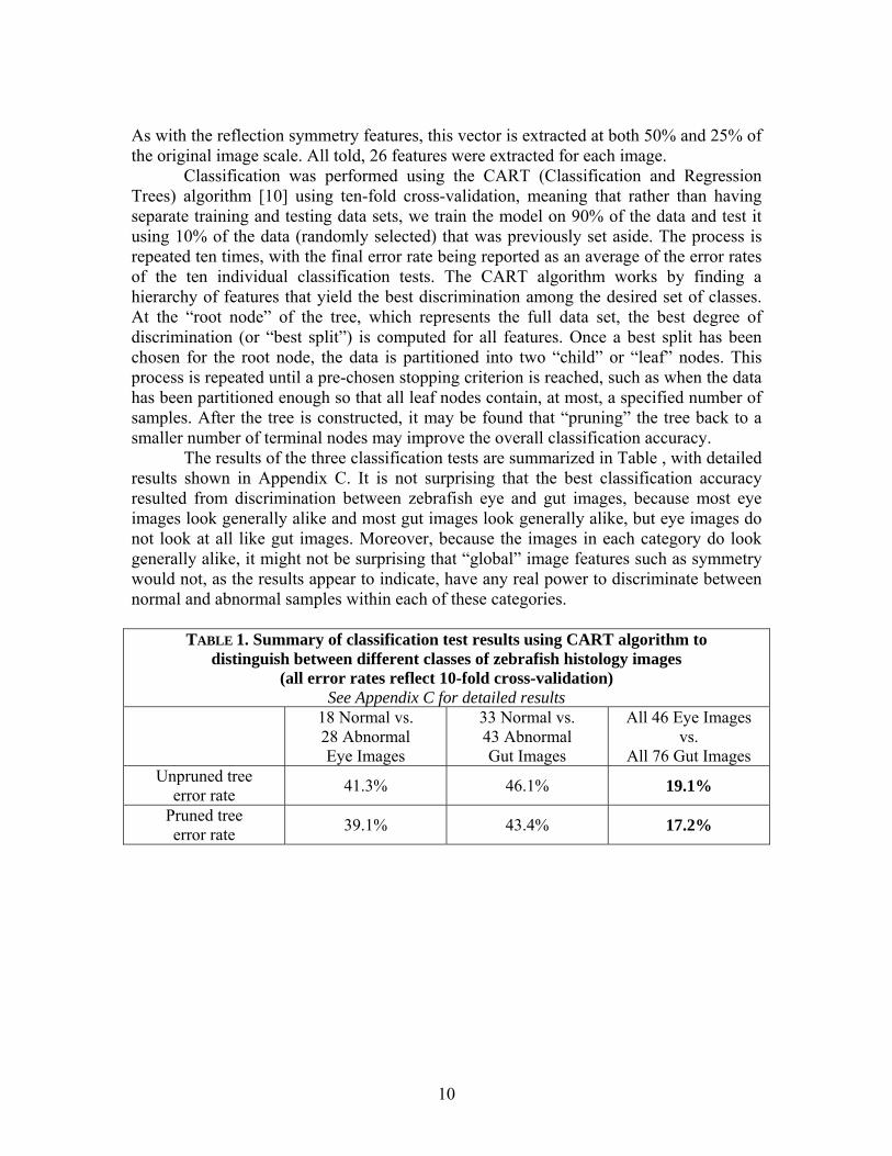
The results of the three classification tests are summarized in Table , with detailed results shown in Appendix C. It is not surprising that the best classification accuracy resulted from discrimination between zebrafish eye and gut images, because most eye images look generally alike and most gut images look generally alike, but eye images do not look at all like gut images. Moreover, because the images in each category do look generally alike, it might not be surprising that “global” image features such as symmetry would not, as the results appear to indicate, have any real power to discriminate between normal and abnormal samples within each of these categories.
TABLE 1. Summary of classification test results using CART algorithm to distinguish between different classes of zebrafish histology images
(all error rates reflect 10-fold cross-validation) See Appendix C for detailed results
18 Normal vs. 28 Abnormal Eye Images
33 Normal vs. 43 Abnormal Gut Images
All 46 Eye Images vs.
All 76 Gut Images Unpruned tree
error rate 41.3% 46.1% 19.1%
Pruned tree error rate 39.1% 43.4% 17.2%
10
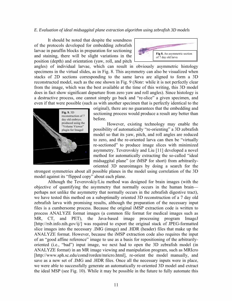
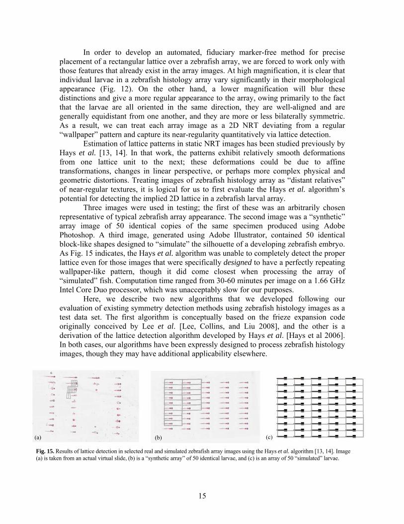
E. Evaluation of ideal midsaggital plane extraction algorithm using zebrafish 3D models
It should be noted that despite the soundness of the protocols developed for embedding zebrafish larvae in paraffin blocks in preparation for sectioning and staining, there will be slight variations in the position (depth) and orientation (yaw, roll, and pitch angles) of individual larvae, which can result in obviously asymmetric histology specimens in the virtual slides, as in Fig. 8. This asymmetry can also be visualized when stacks of 2D sections corresponding to the same larva are aligned to form a 3D reconstructed model, such as the one shown in Fig. 9 (Note: while it is not perfectly clear from the image, which was the best available at the time of this writing, this 3D model does in fact show significant departure from zero yaw and roll angles). Since histology is a destructive process, one cannot simply go back and “re-slice” a given specimen, and even if that were possible (such as with another specimen that is perfectly identical to the
original), there are no guarantees that the embedding and sectioning process would produce a result any better than before.
Fig 8. An asymmetric section of 7 day old larva
However, existing technology may enable the possibility of automatically “re-orienting” a 3D zebrafish model so that its yaw, pitch, and roll angles are reduced to zero, and the re-oriented larva can then be “virtually re-sectioned” to produce image slices with minimized asymmetry. Teverovskiy and Liu [11] developed a novel method for automatically extracting the so-called “ideal midsaggital plane” (or iMSP for short) from arbitrarily-oriented 3D neuroimages by doing a search for the
strongest symmetries about all possible planes in the model using correlation of the 3D model against its “flipped copy” about each plane.
Fig. 9. 3D reconstruction of 7 day old embryo; produced using the “Volume Viewer” plugin for ImageJ
Although the Teverovskiy/Liu method was designed for brain images (with the objective of quantifying the asymmetry that normally occurs in the human brain—perhaps not unlike the asymmetry that normally occurs in the zebrafish digestive tract), we have tested this method on a suboptimally oriented 3D reconstruction of a 7 day old zebrafish larva with promising results, although the preparation of the necessary input files is a cumbersome process. Because the original iMSP extraction code is written to process ANALYZE format images (a common file format for medical images such as MR, CT, and PET), the Java-based image processing program ImageJ [http://rsb.info.nih.gov/ij/] was required to export the original stack of JPEG-formatted slice images into the necessary .IMG (image) and .HDR (header) files that make up the ANALYZE format. However, because the iMSP extraction code also requires the input of an “good affine reference” image to use as a basis for repositioning of the arbitrarily-oriented (i.e., “bad”) input image, we next had to open the 3D zebrafish model (in ANALYZE format) in an MR image viewing and manipulation program, such as MRIcro [http://www.sph.sc.edu/comd/rorden/mricro.html], re-orient the model manually, and save as a new set of .IMG and .HDR files. Once all the necessary inputs were in place, we were able to successfully generate an automatically re-oriented 3D model and extract the ideal MSP (see Fig. 10). While it may be possible in the future to fully automate this
11

workflow, the returns may not always justify the investment of time and resources. Usually, any given larval array consists of multiple specimens of the same genotype (and hence similar histology). In other words, if one specimen is not properly oriented, yielding histology sections too asymmetric to be useful for accurate phenotyping, there is probably another specimen of the same genotype whose sections are more symmetric and arguably more informative.
Before MSP extraction After MSP extraction and re-orientation
Original mid-saggital plane
(specimen is upside down in the reconstructed model due to stacked images being in inverted order)
Ideal mid-saggital plane
Original mid-coronal plane
New mid-coronal plane, “re-sliced” with corrected yaw and roll angles
Fig. 10. Example image sections prior to and following extraction and re-orientation of the larva’s ideal midsaggital plane (iMSP).
12

F. Evaluation of lattice detection algorithms using zebrafish larval array images
Near-regular texture (NRT) is defined [12] as minor geometric, photometric, and topological deformations from an otherwise translationally symmetric 2D wallpaper pattern. NRT can be ubiquitously observed in both man-made and natural objects and their images, such as a checkerboard pattern on a wrinkled tablecloth, a brick wall with color and texture variations among the individual bricks, the hexagonal cells of natural honeycomb, or the scales that make up the curved surface of a fish or shark.
In many real world image patterns, we have observed significant departures from regularity, with large gaps in the NRT pattern that give it a “sparse” appearance (Fig. 11) or severe differences among texels of the same NRT (Fig. 12), such that the current state of the art automatic lattice detection algorithm [13, 14] appears inadequate to extract the implied complete lattice (Fig. 13). On the other hand, certain application-specific cues can be used to enhance the reliability of automatic lattice extraction. Here, we introduce a new method for 2D lattice detection that accounts for sparse and irregular NRT while taking advantage of unique spatial constraints in array images of zebrafish histology.
Fig. 11. The input zebrafish histology image: The challenge here is to estimate the 2D lattice structure implied in fiduciary marker-free, near-regular, sparse, and noisy zebrafish histology images such as that shown above.
Fig. 12. Selected specimens from Fig. 1 at higher magnification, illustrating the typical differences among “texels” (tiles) of the same 2D “wallpaper” pattern.
Significant progress has been made in the automated detection of NRT patterns, whether static [12, 13, 14] or in motion [15]. The detection algorithms used in these works are based on wallpaper group theory [16] in that the topology of such patterns can be characterized completely by a quadrilateral “lattice” composed of fundamental generating units, called texels or textons. Indeed, regular quadrilateral lattices can be represented sufficiently by only two linearly independent vectors.
Fig. 13. Output from our algorithm: The lattice overlaid on the rotation-corrected input array image is detected by exploiting the topological 2D lattice structure and maximizing bilateral symmetry of the zebrafish larva in each lattice cell.
13

Although we have previously developed a prototype system for automatically scoring histological abnormalities in zebrafish organ images [5], the manual image pre-processing required to prepare such images is arguably even more time-consuming than manual image annotation. The first (and slowest) step in pre-processing involves the extraction of specimens from the original virtual slides and then matching each specimen to its corresponding entry in the laboratory’s embedding record, which keeps track of the age and general classification (normal, mutant, or unknown) of the specimens embedded in a particular tissue block (Fig. 14). Certainly, an automated method for specimen extraction would improve the rate of overall throughput in the histology workflow, but the nature of the slide preparation process introduces a number of obstacles that such a method must account for.
Fig. 14. The most time-consuming task in the manual pre-processing of histology array images is the extraction of individual specimen images from the original virtual slides and matching them to their corresponding positions in the laboratory embedding record. Our algorithm enables the automation of much of this task.
In the ideal case of a virtual slide with a perfectly horizontally-oriented
rectangular array of 50 visible specimens and no artifacts or background noise, the extraction process would simply involve locating a rigid 10 row by 5 column lattice with each lattice unit cell bound to its corresponding position on the embedding record. Because of variability in both experimental design and in the handling and preparation of glass slides prior to digitization, such an ideal case is rarely achieved. Sections are often mounted on the slide at a slight angle, dust and other artifacts may be present, and since tissue block embedding depths often vary from specimen to specimen, a particular section may not appear to contain specimens in all positions, giving the array an irregular or sparse structure (Fig. 11).
Perhaps the problem could be solved through the use of fiduciary markers, which if embedded properly could provide a built-in set of interest points or landmarks to assist the computer in detecting the rectangular boundary around the larval array. For example, a certain type of hair or other thin filamentous material could be embedded at each corner of the tissue block to demarcate the array boundary, which would be especially helpful for highly irregular sections. However, the manual process of preparing and slicing a tissue block is already error-prone; including an additional step of embedding fiduciary markers so that they remain normal to the slide surface and do not shift position or cause tearing or wrinkling during the sectioning process is not only impractical but further increases the likelihood of error.
14
In order to develop an automated, fiduciary marker-free method for precise placement of a rectangular lattice over a zebrafish array, we are forced to work only with those features that already exist in the array images. At high magnification, it is clear that individual larvae in a zebrafish histology array vary significantly in their morphological appearance (Fig. 12). On the other hand, a lower magnification will blur these distinctions and give a more regular appearance to the array, owing primarily to the fact that the larvae are all oriented in the same direction, they are well-aligned and are generally equidistant from one another, and they are more or less bilaterally symmetric. As a result, we can treat each array image as a 2D NRT deviating from a regular “wallpaper” pattern and capture its near-regularity quantitatively via lattice detection.
Estimation of lattice patterns in static NRT images has been studied previously by Hays et al. [13, 14]. In that work, the patterns exhibit relatively smooth deformations from one lattice unit to the next; these deformations could be due to affine transformations, changes in linear perspective, or perhaps more complex physical and geometric distortions. Treating images of zebrafish histology array as “distant relatives” of near-regular textures, it is logical for us to first evaluate the Hays et al. algorithm’s potential for detecting the implied 2D lattice in a zebrafish larval array.
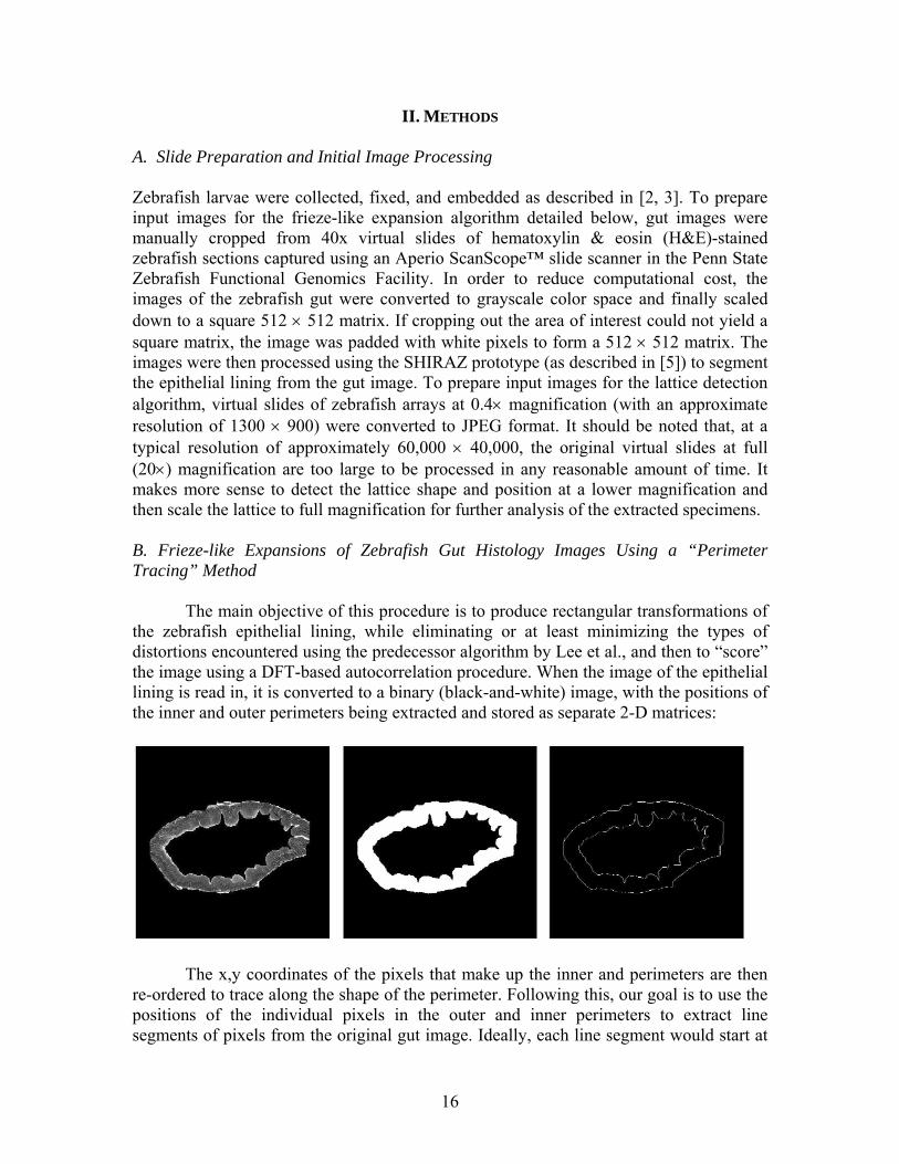
Three images were used in testing; the first of these was an arbitrarily chosen representative of typical zebrafish array appearance. The second image was a “synthetic” array image of 50 identical copies of the same specimen produced using Adobe Photoshop. A third image, generated using Adobe Illustrator, contained 50 identical block-like shapes designed to “simulate” the silhouette of a developing zebrafish embryo. As Fig. 15 indicates, the Hays et al. algorithm was unable to completely detect the proper lattice even for those images that were specifically designed to have a perfectly repeating wallpaper-like pattern, though it did come closest when processing the array of “simulated” fish. Computation time ranged from 30-60 minutes per image on a 1.66 GHz Intel Core Duo processor, which was unacceptably slow for our purposes.
Here, we describe two new algorithms that we developed following our evaluation of existing symmetry detection methods using zebrafish histology images as a test data set. The first algorithm is conceptually based on the frieze expansion code originally conceived by Lee et al. [Lee, Collins, and Liu 2008], and the other is a derivation of the lattice detection algorithm developed by Hays et al. [Hays et al 2006]. In both cases, our algorithms have been expressly designed to process zebrafish histology images, though they may have additional applicability elsewhere.
(c) (a) (b)
Fig. 15. Results of lattice detection in selected real and simulated zebrafish array images using the Hays et al. algorithm [13, 14]. Image (a) is taken from an actual virtual slide, (b) is a “synthetic array” of 50 identical larvae, and (c) is an array of 50 “simulated” larvae.
15
II. METHODS
A. Slide Preparation and Initial Image Processing Zebrafish larvae were collected, fixed, and embedded as described in [2, 3]. To prepare input images for the frieze-like expansion algorithm detailed below, gut images were manually cropped from 40x virtual slides of hematoxylin & eosin (H&E)-stained zebrafish sections captured using an Aperio ScanScope™ slide scanner in the Penn State Zebrafish Functional Genomics Facility. In order to reduce computational cost, the images of the zebrafish gut were converted to grayscale color space and finally scaled down to a square 512 × 512 matrix. If cropping out the area of interest could not yield a square matrix, the image was padded with white pixels to form a 512 × 512 matrix. The images were then processed using the SHIRAZ prototype (as described in [5]) to segment the epithelial lining from the gut image. To prepare input images for the lattice detection algorithm, virtual slides of zebrafish arrays at 0.4× magnification (with an approximate resolution of 1300 × 900) were converted to JPEG format. It should be noted that, at a typical resolution of approximately 60,000 × 40,000, the original virtual slides at full (20×) magnification are too large to be processed in any reasonable amount of time. It makes more sense to detect the lattice shape and position at a lower magnification and then scale the lattice to full magnification for further analysis of the extracted specimens.
B. Frieze-like Expansions of Zebrafish Gut Histology Images Using a “Perimeter Tracing” Method
The main objective of this procedure is to produce rectangular transformations of the zebrafish epithelial lining, while eliminating or at least minimizing the types of distortions encountered using the predecessor algorithm by Lee et al., and then to “score” the image using a DFT-based autocorrelation procedure. When the image of the epithelial lining is read in, it is converted to a binary (black-and-white) image, with the positions of the inner and outer perimeters being extracted and stored as separate 2-D matrices:
The x,y coordinates of the pixels that make up the inner and perimeters are then re-ordered to trace along the shape of the perimeter. Following this, our goal is to use the positions of the individual pixels in the outer and inner perimeters to extract line segments of pixels from the original gut image. Ideally, each line segment would start at
16

the outer perimeter and be oriented more or less perpendicular to the line tangent to the outer perimeter, with the endpoint of the line segment being the intersecting point on the inner perimeter. However, owing to the irregular shape of the both perimeters, the line segment may not necessarily end at the desired point on the inner perimeter; in fact, in some cases the line perpendicular to the tangent line at the starting point may not even intersect with the inner perimeter at all. To remedy this, we choose a set of initial control points evenly spaced around the outer perimeter. (By default, the algorithm will choose 12 such points.) Line segments are drawn from these control points to the nearest point on the inner perimeter as measured by Euclidean distance. This, in effect, divides the lining into a series of “sections” that we can process individually:
For each individual section, we compute the ratio of the number of pixels on the inner perimeter divided by the number of pixels on the outer perimeter. We then extract line segments starting from each pixel on the outer perimeter and ending at the inner perimeter pixel location, which is determined by multiplying the inner-to-outer perimeter ratio by the current outer perimeter position, and then rounding up to the nearest integer. It should be noted that since the number of pixels on the inner perimeter in a given section may be greater than or less than the corresponding number of pixels on the outer perimeter, one may find that either not every inner perimeter pixel is used or that certain inner perimeter pixels are used more than once. The line segment extractions are then repeated for all of the individual sections. In a sense, we are “interpolating” the extraction of line segments from each section based on the positions of line segments located at the initial control points (here, we show a subset of the extracted line segments for illustrative purposes only):
17
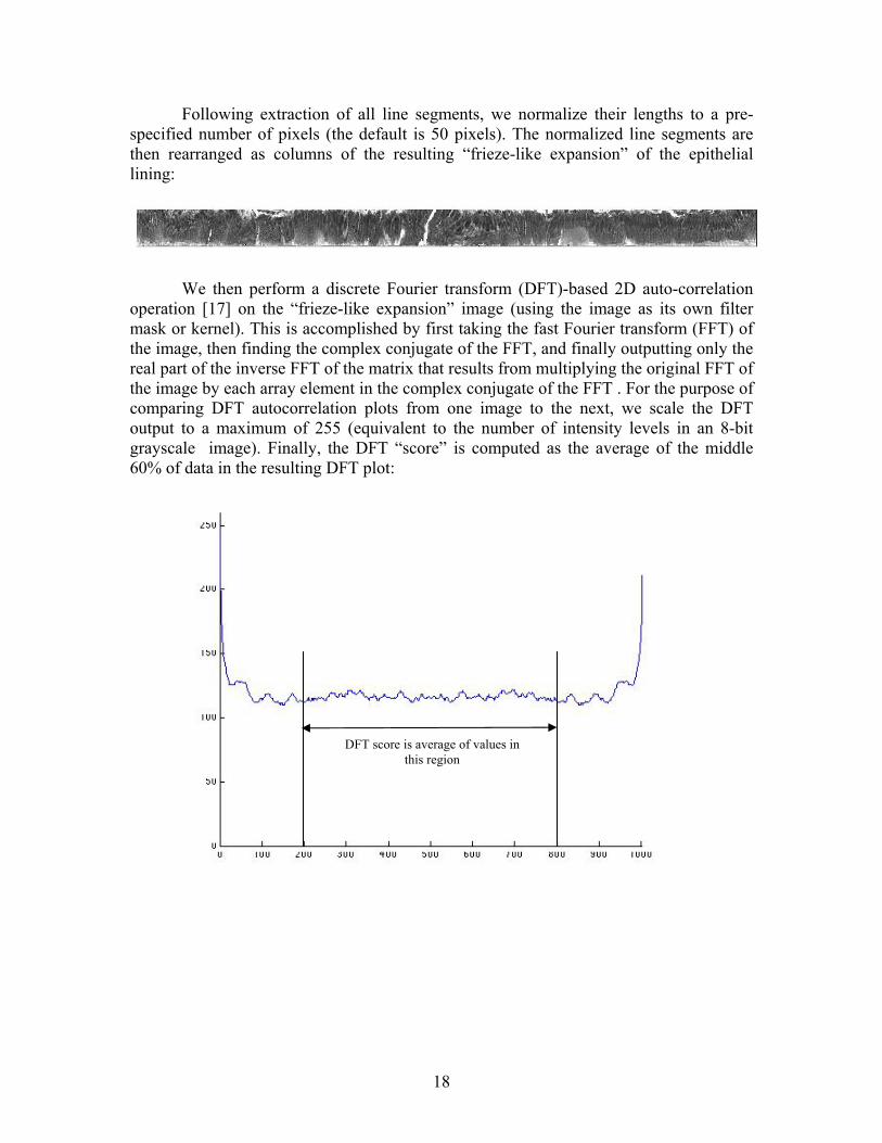
Following extraction of all line segments, we normalize their lengths to a pre-specified number of pixels (the default is 50 pixels). The normalized line segments are then rearranged as columns of the resulting “frieze-like expansion” of the epithelial lining:
We then perform a discrete Fourier transform (DFT)-based 2D auto-correlation operation [17] on the “frieze-like expansion” image (using the image as its own filter mask or kernel). This is accomplished by first taking the fast Fourier transform (FFT) of the image, then finding the complex conjugate of the FFT, and finally outputting only the real part of the inverse FFT of the matrix that results from multiplying the original FFT of the image by each array element in the complex conjugate of the FFT . For the purpose of comparing DFT autocorrelation plots from one image to the next, we scale the DFT output to a maximum of 255 (equivalent to the number of intensity levels in an 8-bit grayscale image). Finally, the DFT “score” is computed as the average of the middle 60% of data in the resulting DFT plot:
DFT score is average of values in this region
18

C. Lattice Detection for Zebrafish Larval Histology Arrays Our algorithm proceeds in three stages. In stage 1 (Figs. 16a,b), the rotation offset of the array image, if any, is corrected so that all specimens are oriented horizontally. In stage 2 (Figs. 16c,d), we use the detected number of cells in the array to divide the bounding box circumscribing the specimens into an initial lattice, taking advantage of the upper bounds of 5 columns and 10 rows imposed by the histology array apparatus design. In practice, we have observed that is it sufficient to assume that the lattice will contain ten rows, even if some rows are partially or totally unoccupied. The number of columns in the field of view, however, will vary from 1 to 5 depending on the design of that particular histology experiment. Finally, in stage 3 (Fig. 16e), we optimize the initial lattice by varying its height until we maximize the symmetry of each lattice cell image about its horizontal reflection axis. The algorithm pseudocode is provided as follows:
Stage 1: Global orientation correction
1 Aconvhull = area of convex hull around array specimens 2 Abox = area of bounding box around convex hull 3 θcorrected = argmax (Aconvhull / Abox )
Stage 2: Rigid lattice placement
4 Perform morphological closing operation 5 ncolumns = number of connected components 6 nrows = 10 (assumed) 7 Linitial = result of dividing bounding box around foreground pixels into lattice with
(nrowsncolumns) equally sized cells
Stage 3: Deformable lattice optimization
8 For each grayscale cell image C in lattice L 9 S = corr(C, mirrorimage(C)) 10 Lfinal =argmax(S) for all C
Fig. 16. Illustration of our new lattice detection algorithm. In (a), the convex hull around the array specimens is rotated until the fraction of the bounding box area occupied by the convex hull is maximized as in (b), noting that the bounding box “shrinks” to fit the convex hull as it rotates. In (c), the number of columns is determined by a morphological closing operation. The bounding box is then divided into the initial lattice (d), which is optimized by varying the lattice height until the reflective symmetry in each cell is maximized (e).
19

III. RESULTS AND DISCUSSION A. Frieze-like expansion of gut images using perimeter tracing The algorithm was used to process 34 images of zebrafish gut epithelia that had been previously segmented from their original gut images using the SHIRAZ prototype [5]. 16 of these images represented normal or wild-type guts, and the remaining 18 represented abnormal or mutant tissue. A subset of these images, along with their corresponding frieze-like expansions and DFT autocorrelation plots, is shown in the tables below. (All average DFT scores provided are calculated over the middle 60% of the values that make up the DFT plot. For example, in the first plot, which consists of 1000 points, we average the scaled score from position 200 to position 800.)
Image filename: gut-wt1841B-b1-2-5dpf-wt-3_lining.jpg (normal)
Original gut image (with example
line segment extractions) Resulting DFT autocorrelation plot (Average DFT score = 116.5439)
Frieze-like expansion following extraction and normalization of line segments
20

Image filename: gut-wt5d-11may2007-13218-1.jpg_lining.jpg (normal)
Original gut image (with example
line segment extractions) Resulting DFT autocorrelation plot
(Average DFT score = 70.3017)
Frieze-like expansion following extraction and normalization of line segments
Image filename: gut-wt5d-11may2007-13219-2.jpg_lining.jpg (normal)
Original gut image (with example
line segment extractions) Resulting DFT autocorrelation plot (Average DFT score = 100.6835)
Frieze-like expansion following extraction and normalization of line segments
21

Image filename: gut-mu3308-b5-2-5dpf-1_lining.jpg (mutant)
Original gut image (with example line
segment extractions) Resulting DFT autocorrelation plot
(Average DFT score = 14.1466)
Frieze-like expansion following extraction and normalization of line segments
Image filename: gut-mu1437-3439-1-9-4dpf-2_lining.jpg (mutant)
Original gut image (with example line
segment extractions) Resulting DFT autocorrelation plot
(Average DFT score = 55.4545)
Frieze-like expansion following extraction and normalization of line segments
22

Image filename: gut-mu2735A-b1-2-5dpf-2_lining.jpg (mutant)
Original gut image (with example line segment extractions)
Resulting DFT autocorrelation plot (Average DFT score = 16.0787)
Frieze-like expansion following extraction and normalization of line segments
Image filename: gut-mu3644-b2-7-5dpf-7_lining.jpg (mutant)
Original gut image (with example line segment extractions)
Resulting DFT autocorrelation plot (Average DFT score = 42.8513)
Frieze-like expansion following extraction and normalization of line segments
23

The DFT scores for all 34 images tested (including those above) are summarized in the table below: Image Filename Class DFT score gut-wt1841B-b1-2-5dpf-wt-3_lining.jpg wild-type 116.5439
gut-wt5d-11may2007-13218-1.jpg_lining.jpg wild-type 70.3017
gut-wt5d-11may2007-13219-1.jpg_lining.jpg wild-type 97.076
gut-wt5d-11may2007-13219-2.jpg_lining.jpg wild-type 100.6835
gut-wt5d-11may2007-13219-4.jpg_lining.jpg wild-type 24.4761
gut-wt5d-11may2007-13220-1.jpg_lining.jpg wild-type 43.9393
gut-wt5d-11may2007-13220-3.jpg_lining.jpg wild-type 19.9616
gut-wt5d-11may2007-13221-1.jpg_lining.jpg wild-type 49.4734
gut-wt5d-11may2007-13221-2.jpg_lining.jpg wild-type 30.6004
gut-wt5d-11may2007-13221-3.jpg_lining.jpg wild-type 41.2855
gut-wt5d-11may2007-13221-4-31pt6X.jpg_lining.jpg wild-type 81.4948
gut-wt7d-12may2007-13239-1.jpg_lining.jpg wild-type 34.5978
gut-wt7d-12may2007-13239-2-33pt6.jpg_lining.jpg wild-type 32.6226
gut-wt7d-12may2007-13240-2-33pt6.jpg_lining.jpg wild-type 23.1009
gut-wt7d-12may2007-13240-3-33pt6.jpg_lining.jpg wild-type 22.305
gut-wt7d-12may2007-13241-1.jpg_lining.jpg wild-type 22.3086
gut-mu3308-b5-2-5dpf-1_lining.jpg mutant 14.1466
gut-mu1437-3439-1-9-4dpf-2_lining.jpg mutant 55.4545
gut-mu2735A-b1-2-5dpf-2_lining.jpg mutant 16.0787
gut-mu3644-b2-7-5dpf-7_lining.jpg mutant 42.8513
gut-mu-blindsided_lining.jpg mutant 11.6888
gut-mu318-b1-2-5dpf-mu-1_lining.jpg mutant 68.7201
gut-mu383a-b1-5-C4-4dpf-10_lining.jpg mutant 59.5793
gut-mu559-b1_4-C4_4dpf-6_lining.jpg mutant 23.8504
gut-mu800a-b1-10-C2-4dpf-4_lining.jpg mutant 49.9693
gut-mu962-2019-b1-2-5dpf-5_lining.jpg mutant 29.4484
gut-mu559-b1-3-C4-4dpf_lining.jpg mutant 19.2524
gut-mu975-b2-1-5dpf-1_lining.jpg mutant 19.2126
gut-mu1143-b1-4-4dpf-4_lining.jpg mutant 22.4149
gut-mu1364BND-b1-3-4dpf-6_lining.jpg mutant 15.5947
gut-mu1482-b2-3-5dpf-4_lining.jpg mutant 22.9089
gut-mu1743-b1-11-C4-4dpf-20_lining.jpg mutant 54.71
gut-mu1903C-b1-C1-5dpf-2_lining.jpg mutant 17.3687
gut-mu2404-b1-1-5dpf-4_lining.jpg mutant 18.8074
gut-mu2914-b1-4-4dpf-6_lining.jpg mutant 16.6387
Mean DFT score for wild-type images: μW = 50.673 Standard deviation: 32.093 Mean DFT score for mutant images: μM = 30.458 Standard deviation: 18.290
If we take our null hypothesis to be that μM = μW, then a one-tailed, two-sample, unequal-variance Student’s t-test performed on the data set results in a P-value of 0.0178, which by most standards is small enough to reject the null hypothesis and conclude that the mean DFT value of the mutant (abnormal) images is significantly less than that of the
24
normal (wild-type) images. (For the sake of completeness, a two-tailed test doubles the P-value to 0.0356, which is still low enough to reject the null hypothesis.) Therefore, our initial hypothesis that DFT score can be used to help discriminate between normal and abnormal tissues may have some validity, although these results would certainly be more conclusive with a much larger set of images (we would prefer to have at least 30 images in each group for significance testing). Since the data show some degree of overlap in DFT values between the two classes, it is clear that DFT alone cannot be used to predict the class of a previously-unclassified image; however, perhaps better results might arise by training a classifier with not only DFT scores but also with other features that can be easily extracted from these images (e.g., gray-level co-occurrence matrix properties for quantifying image texture [18]). Finally, execution time in all cases was 30 seconds or less, and as low as 10 seconds for some images.
25

B. Lattice detection in zebrafish larval arrays
Our algorithm was tested on a set of twenty different virtual slide images. These were chosen to be representative of the types of variation one can expect to observe, including differences in overall array shape and orientation, number and sparsity of specimens, quality of sections, as well as background noise and other image artifacts such as dust particles. In comparison to the 30-60 minutes required for processing by the Hays et al. algorithm [13,14], the computation time for a typical 1300 × 900 image using our method was less than 5 minutes using a 1.66 GHz Intel Core Duo processor. However, reducing the image dimensions by 50% (from 1300 × 900 to 650 × 450, for example) yielded a substantially improved computation time of about one minute or less, although results can vary depending on the step sizes used in the rotation correction and lattice optimization routines as well as the number and size of individual cells detected in the lattice. Example outputs are shown in Fig. 17.
100% lattice detection accuracy was achieved in 19 of the 20 images tested—even those with significant noise and artifacts (e.g., Fig. 17a). One image yielded 85% accuracy (Fig. 17c), which we attribute to the translational symmetry within the wallpaper pattern being distorted, in that some larvae appear to have shifted from their original positions due to improper tissue block preparation and sectioning. See Appendix D for detection results for all twenty images.
(b)(a) (c)
Fig. 17. Selected output images as processed by our lattice detection algorithm. In the vast majority of tests, as with (a) and (b), the algorithm detected lattices with 100% accuracy. Note that the barely-visible specimen in the upper right corner of (a) was detected even with significant image noise. Lattice detection was suboptimal for (c) as a result of specimen shifting due to improper sectioning.
26
IV. CONCLUSIONS AND FUTURE WORK
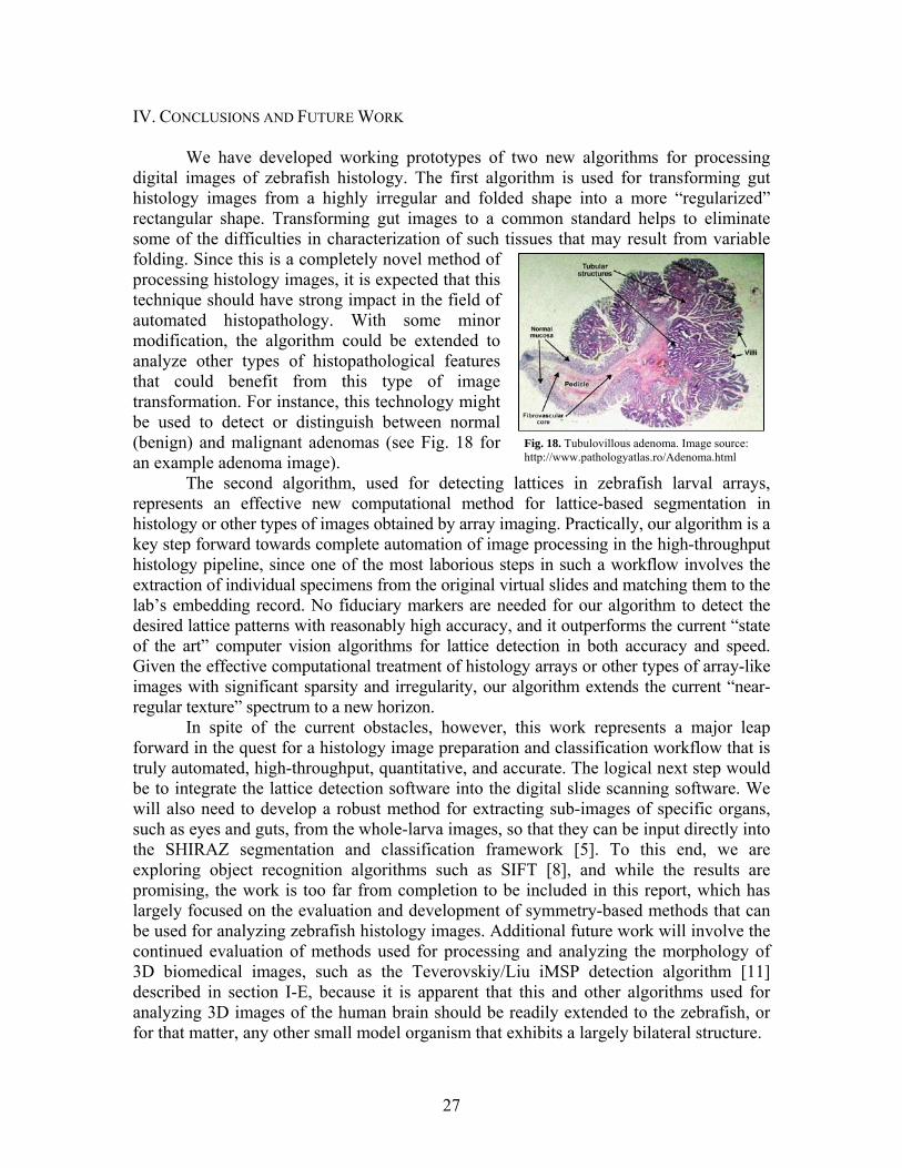
We have developed working prototypes of two new algorithms for processing digital images of zebrafish histology. The first algorithm is used for transforming gut histology images from a highly irregular and folded shape into a more “regularized” rectangular shape. Transforming gut images to a common standard helps to eliminate some of the difficulties in characterization of such tissues that may result from variable folding. Since this is a completely novel method of processing histology images, it is expected that this technique should have strong impact in the field of automated histopathology. With some minor modification, the algorithm could be extended to analyze other types of histopathological features that could benefit from this type of image transformation. For instance, this technology might be used to detect or distinguish between normal (benign) and malignant adenomas (see Fig. 18 for an example adenoma image).
Fig. 18. Tubulovillous adenoma. Image source: http://www.pathologyatlas.ro/Adenoma.html
The second algorithm, used for detecting lattices in zebrafish larval arrays, represents an effective new computational method for lattice-based segmentation in histology or other types of images obtained by array imaging. Practically, our algorithm is a key step forward towards complete automation of image processing in the high-throughput histology pipeline, since one of the most laborious steps in such a workflow involves the extraction of individual specimens from the original virtual slides and matching them to the lab’s embedding record. No fiduciary markers are needed for our algorithm to detect the desired lattice patterns with reasonably high accuracy, and it outperforms the current “state of the art” computer vision algorithms for lattice detection in both accuracy and speed. Given the effective computational treatment of histology arrays or other types of array-like images with significant sparsity and irregularity, our algorithm extends the current “near-regular texture” spectrum to a new horizon.
In spite of the current obstacles, however, this work represents a major leap forward in the quest for a histology image preparation and classification workflow that is truly automated, high-throughput, quantitative, and accurate. The logical next step would be to integrate the lattice detection software into the digital slide scanning software. We will also need to develop a robust method for extracting sub-images of specific organs, such as eyes and guts, from the whole-larva images, so that they can be input directly into the SHIRAZ segmentation and classification framework [5]. To this end, we are exploring object recognition algorithms such as SIFT [8], and while the results are promising, the work is too far from completion to be included in this report, which has largely focused on the evaluation and development of symmetry-based methods that can be used for analyzing zebrafish histology images. Additional future work will involve the continued evaluation of methods used for processing and analyzing the morphology of 3D biomedical images, such as the Teverovskiy/Liu iMSP detection algorithm [11] described in section I-E, because it is apparent that this and other algorithms used for analyzing 3D images of the human brain should be readily extended to the zebrafish, or for that matter, any other small model organism that exhibits a largely bilateral structure.
27

ACKNOWLEDGEMENTS
This work was funded by the Penn State Academic Computing Fellowship and was an extension of the course project work from the Penn State Computer Science and Engineering (CSE 398B) Fall 2007 course on Computational Symmetry, taught by Professor Liu. The authors gratefully acknowledge Georgia Thomas and Keith Cheng (both at the Penn State College of Medicine) for providing image data, domain knowledge and useful feedback. We would also thank James Z. Wang (Penn State College of Information Sciences & Technology) for helpful comments.
REFERENCES [1] C. Nusslein-Volhard, and R. Dahm (eds.), Zebrafish: A Practical Approach,
Oxford: Oxford University Press; 2002. [2] G.S. Tsao-Wu, C.H Weber, L.R. Budgeon, and K.C. Cheng, Agarose embedded
tissue arrays for histologic and genetic analysis, Biotechniques, vol. 25, pp 614-618, 1998.
[3] N.A. Sabaliauskas, C.A. Foutz, et al., High-throughput zebrafish histology.
Methods, vol. 39, pp 246-254, 2006. [4] P. Colquhoun, J.J. Nogueras, et al., Interobserver and intraobserver bias exists in
the interpretation of anal dysplasia. Dis Colon Rectum, vol. 46, pp 1332-1338, 2003.
[5] B.A. Canada, G.K. Thomas, K.C. Cheng, and J.Z. Wang, Automated
Segmentation and Classification of Zebrafish Histology Images for High-Throughput Phenotyping, Proceedings of the Third IEEE-NIH Life Science Systems and Applications Workshop, pp. 245-248, 2007.
[6] Y. Liu, J.H. Hays, Y. Xu, and H. Shum, Digital Papercutting, Technical Sketch,
SIGGRAPH, 2005. [7] G. Loy, J. Eklundh, Detecting Symmetry and Symmetric Constellations of
Features, 9th European Conference on Computer Vision, vol. 2, pp 508-521, 2006.
[8] D.G. Lowe, Distinctive image features from scale-invariant keypoints,
International Journal of Computer Vision, vol. 2, pp. 91-110, 2004. [9] V.S.N. Prasad, L.S. Davis, Detecting rotational symmetries, Tenth IEEE
International Conference on Computer Vision, vol. 2, pp 954 – 961, 2005. [10] L. Breiman, J. Friedman, C.J. Stone, and R.A. Olshen, Classification and
Regression Trees, Belmont: Wadsworth International Group; 1984.
28

[11] L. Teverovskiy and Y. Liu, Truly 3D Midsagittal Plane Extraction for Robust
Neuroimage Registration, 3rd IEEE International Symposium on Biomedical Imaging: Macro to Nano, pp. 860 - 863, 2006.
[12] Y. Liu, R. Collins, and Y. Tsin, A Computational Model for Periodic Pattern
Perception Based on Frieze and Wallpaper Groups, IEEE Trans. Pattern Analysis and Machine Intelligence, Vol. 26, No. 3, pp. 354 – 371, 2004.
[13] J.H. Hays, M. Leordeanu, A.A. Efros, and Y. Liu, Discovering Texture Regularity
as a Higher-Order Correspondence Problem, 9th European Conference on Computer Vision, 2006.
[14] Y. Liu, W. Lin, and J.H. Hays, Near Regular Texture Analysis and Manipulation,
ACM Transactions on Graphics (SIGGRAPH 2004), Vol. 23, No. 3, pp. 368-376, 2004.
[15] W. Lin and Y. Liu, A Lattice-based MRF Model for Dynamic Near-regular
Texture Tracking, IEEE Trans. Pattern Analysis and Machine Intelligence, Vol. 29, No. 5, pp. 777-792, 2007.
[16] B. Grünbaum and G.C. Shephard, Tilings and Patterns, New York: W. H.
Freeman and Company, 1987. [17] R.C. Gonzalez, R.E. Woods, S.L. Eddins, Digital Image Processing using
MATLAB, Upper Saddle River, N. J. : Pearson Prentice Hall; 2004. [18] R.M. Haralick, K. Shanmugam, I. Dinstein, Texture features for image
classification. IEEE Transactions on Systems, Man, and Cybernetics. vol. 3, pp 610-621, 1973.
[19] S. Lee, R. T. Collins and Y. Liu, Rotation Symmetry Group Detection Via Frequency Analysis of Frieze-Expansions," Computer Vision and Pattern Recognition Conference (CVPR '08), June 2008.
29

Appendix A — Results from evaluation of state-of-the-art reflection and rotation symmetry detection algorithms
Ground Truth
(Bilateral symmetry axes = yellow, local centers of
rotation = green star)
Loy (Bilateral)
Loy (Rotational
) Prasad Liu
14521-C3R8-head
T/F = True/False,
P/N = Positive/Negative,
PPV=Positive Predictive Value=TP/(TP+FP),
Sensitivity=TP/(TP+FN)
TP=2,FP=3,FN=1 PPV=40%,Sensitivity=67%
TP=0,FP=3,FN=1 PPV=0%,Sensitivity=0%
TP=1,FP=1,FN=0 PPV=50%,Sens=100%
TP=1,FP=1,FN=1 PPV=100%,Sens.=50%
14521-C3R8-whole
Nothing detected
TP=1,FP=0,FN=0 PPV=100%,Sensitivity=10
0%
TP=0,FP=2,FN=0 PPV=0%,Sensitivity=0%
TP=0,FP=1,FN=0 PPV=0%,Sens=0%
TP=0,FP=0,FN=1 PPV=n/a,Sens.=0%
14558-C1R4
Nothing detected
TP=1,FP=5(?),FN=2 PPV=17%,Sensitivity=33%
TP=0,FP=3,FN=0 PPV=0%,Sensitivity=0%
TP=0,FP=1,FN=0 PPV=0%,Sens=0%
TP=0,FP=0,FN=3 PPV=n/a,Sens.=0%
14558-C1R5
Nothing detected
TP=0,FP=2,FN=1 PPV=0%,Sensitivity=0%
TP=0,FP=3,FN=1 PPV=0%,Sensitivity=0%
TP=1,FP=0,FN=0 PPV=100%,Sens=100%
TP=0,FP=0,FN=1 PPV=n/a,Sens.=0%
14558-C1R6
Nothing detected
30

TP=2,FP=1,FN=1 TP=0,FP=2,FN=2 TP=1,FP=1,FN=1
TP=0,FP=0,FN=3
PPV=67%,Sensitivity=67% PPV=0%,Sensitivity=0% PPV=50%,Sens=50% PPV=n/a,Sens.=0%
14558-C3R8
TP=1,FP=6(?),FN=2
P
TP=1,FP=0,FN=1 PPV=100%,Sensitivity=0 TP=1,FP=0,FN=1
PPV=100%,Sens=50% PPV=100%,Sens.=33% PV=14%,Sensitivity=33% %
TP=1,FP=0,FN=2
14558-C3R8
File accidentally overwritten
Nothing detected
N/A TP=2,FP=1,FN=0
PPV=67%,Sensitivity=10
TP=1,FP=1,FN=1 PPV=50%,Sens=50%
TP=0,FP=0,FN=1 PPV=n/a,Sens.=0%
0%
14558-C3R9
TP=1,FP=1,FN=1
PPV=50%,Sensitivity=50%
TP=1,FP=2,FN=1 PPV=33%,Sensitivity=50 TP=0,FP=1,FN=2
PPV=0%,Sens=0% PPV=100%,Sens.=33% %
TP=1,FP=0,FN=2
14558-C3R9-whole
Nothing detected
TP=1,FP=1(?),FN=0 PPV=50%,Sensitivity=100
TP=2,FP=1,FN=0 PPV=67%,Sensitivity=10 TP=0,FP=1,FN=2
PPV=0%,Sens=0% TP=0,FP=0,FN=1
PPV=N/A,Sens.=0% % 0%
14558-C4R2
(error in C vresult)
n
oting; no
TP=1,FP=0,FN=2 PPV=100%,Sensitivity=33
%
TP=1,FP=2,FN=1 PPV=33%,Sensitivity=50
%
TP=0,FP=4,FN=2 PPV=0%,Sens=0%
TP=1,FP=0,FN=1 PPV=100%,Sens.=50%
31
14558-C4R9-head
(error in Cn voting; no result)
TP=0,FP=2(?),FN=2 PPV=0%,Sensitivity=0%
TP=1,FP=2,FN=0 PPV=33%,Sensitivity=10 FN=1 TP=1,FP=1,FN=0
PPV=50%,Sens.=100% 0%
TP=0,FP=3,PPV=0%,Sens=0%
14558-C4R9-whole
(error in Cn voting; no result)
Nothing detected
TP=0,FP=1(?),FN=0 PPV=0%,Sensitivity=N/A
TP=1,FP=2,FN=0 PPV=33%,Sensitivity=10
TP=0,FP=5,FN=1 PPV=0%,Sens=0%
TP=0,FP=0,FN=0 PPV=N/A,Sens.=N/A 0%
14604-C5R3
TP=1,FP=0,FN=2
PPV=100%,Sensitivity=33
TP=2,FP=1,FN=0 PPV=67%,Sensitivity=10
TP=0,FP=4,FN=2 PPV=0%,Sens=0
TP=1,FP=0,FN=2 PPV=100%,Sens.=33% % 0% %
14604-C5R4
TP=2,FP=0,FN=1
PPV=100%,Sensitivity=67%
TP=0,FP=3,FN=2 PPV=0%,Sensitivity=0%
TP=0,FP=1,FN=2 PPV=0%,Sens=0%
TP=1,FP=0,FN=2 PPV=100%,Sens.=33%
14604-C5R5
(error in Cn voting;
result) no
TP=1,FP=2,FN=2 PPV=33%,Sensitivity=33%
TP=0,FP=2,FN=2 PPV=0%,Sensitivity=0%
TP=0,FP=2,FN=2 PPV=0%,Sens=0%
TP=1,FP=0,FN=2 PPV=100%,Sens.=33%
Overall Comparison
Avg. PPV = 48%
Avg.
Sensitivity = 44%
Avg. PPV = 29%
Avg.
Sensitivity = 40%
Avg. PPV = 23%
Avg.
Sensitivity
= 23%
Avg. PPV = 43%
Avg.
Sensitivity = 24%
32

Appendix B — Additional evalution results for rotation symmetry detection, incorporating the frieze-expansion method of Lee et al.
Ground Truth
(Bilateral symmetry axes = yellow, local centers of
rotation = green star)
Loy (Rotational
) Prasad S. Lee
14521-C3R8-head
T/F = True/False, P/N =
Positive/Negative, PPV=Positive Predictive
Value=TP/(TP+FP), Sensitivity=TP/(TP+FN)
TP=0,FP=3,FN=1 PPV=0%,Sensitivity=0%
TP=1,FP=1,FN=0 PPV=50%,Sens=100%
TP=0,FP=2,FN=1 PPV=0%,Sens.=0%
14558-C1R4
TP=0,FP=3,FN=0 PPV=0%,Sensitivity=0%
TP=0,FP=1,FN=0 PPV=0%,Sens=0%
TP=0,FP=1,FN=2 PPV=0%,Sens.=0%
14558-C1R6
TP=0,FP=2,FN=2 PPV=0%,Sensitivity=0%
TP=1,FP=1,FN=1 PPV=50%,Sens=50%
TP=0,FP=1,FN=2 PPV=0%,Sens.=0%
14558-C3R8
TP=1,FP=0,FN=1 PPV=100%,Sensitivity=0
%
TP=1,FP=0,FN=1 PPV=100%,Sens=50%
TP=0,FP=2,FN=2 PPV=0%,Sens.=0%
33
14558-C4R2
(error in Cn voting; no result)
TP=1,FP=2,FN=1 PPV=33%,Sensitivity=50
%
TP=0,FP=4,FN=2 PPV=0%,Sens=0%
TP=0,FP=1,FN=2 PPV=0%,Sens.=0%
14558-C4R9-head
(error in Cn voting; no result)
TP=1,FP=2,FN=0 PPV=33%,Sensitivity=10
0%
TP=0,FP=3,FN=1 PPV=0%,Sens=0%
TP=0,FP=2,FN=1 PPV=0%,Sens.=0%
14604-C5R3
TP=2,FP=1,FN=0 PPV=67%,Sensitivity=10
0%
TP=0,FP=4,FN=2 PPV=0%,Sens=0%
TP=0,FP=3,FN=2 PPV=0%,Sens.=0%
14604-C5R4
TP=0,FP=3,FN=2 PPV=0%,Sensitivity=0%
TP=0,FP=1,FN=2 PPV=0%,Sens=0%
TP=0,FP=4,FN=2 PPV=0%,Sens.=0%
14604-C5R5
(error in Cn voting; no result)
TP=0,FP=2,FN=2 PPV=0%,Sensitivity=0%
TP=0,FP=2,FN=2 PPV=0%,Sens=0%
TP=0,FP=3,FN=2 PPV=0%,Sens.=0%
Overall Comparison
Avg. PPV = 22%
Avg.
Sensitivity = 36%
Avg. PPV = 15%
Avg.
Sensitivity
= 19%
Avg. PPV = 0%
Avg. Sensitivity = 0%
34

Appendix C — Classification test results using CART algorithm to distinguish between different classes of zebrafish histology images Test 1: 18 normal (wild-type) zebrafish eye images vs. 28 abnormal zebrafish eye images (all of variable age between 3 and 7 days post-fertilization) Original, “un-pruned” classification tree (Class 1 = normal, Class 2 = abnormal)
The features at each node in the tree above correspond to the following: X14 = Maximum rotational symmetry strength at 25% scale X10 = Minimum reflection symmetry strength at 25% scale X17 = Std. deviation of rotational symmetry strength at 25% scale X24 = Std. deviation of rotational symmetry strength at 50% scale X26 = Minimum order of rotational symmetry at 50% scale The error rate (or cost) for the above tree was reported as 41.3%, which is slightly worse than a tree pruned back to the root node (i.e., simply classifying all images as abnormal), with an error rate of 39.1%, which is the best error rate achievable. The corresponding best-pruned tree for this test is shown here:
35
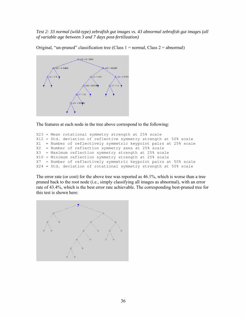
Test 2: 33 normal (wild-type) zebrafish gut images vs. 43 abnormal zebrafish gut images (all of variable age between 3 and 7 days post-fertilization) Original, “un-pruned” classification tree (Class 1 = normal, Class 2 = abnormal)
The features at each node in the tree above correspond to the following: X23 = Mean rotational symmetry strength at 25% scale X12 = Std. deviation of reflective symmetry strength at 50% scale X1 = Number of reflectively symmetric keypoint pairs at 25% scale X2 = Number of reflection symmetry axes at 25% scale X3 = Maximum reflection symmetry strength at 25% scale X10 = Minimum reflection symmetry strength at 25% scale X7 = Number of reflectively symmetric keypoint pairs at 50% scale X24 = Std. deviation of rotational symmetry strength at 50% scale The error rate (or cost) for the above tree was reported as 46.1%, which is worse than a tree pruned back to the root node (i.e., simply classifying all images as abnormal), with an error rate of 43.4%, which is the best error rate achievable. The corresponding best-pruned tree for this test is shown here:
36
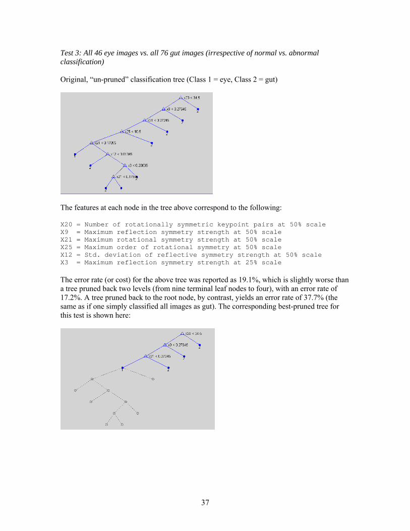
Test 3: All 46 eye images vs. all 76 gut images (irrespective of normal vs. abnormal classification) Original, “un-pruned” classification tree (Class 1 = eye, Class 2 = gut)
The features at each node in the tree above correspond to the following: X20 = Number of rotationally symmetric keypoint pairs at 50% scale X9 = Maximum reflection symmetry strength at 50% scale X21 = Maximum rotational symmetry strength at 50% scale X25 = Maximum order of rotational symmetry at 50% scale X12 = Std. deviation of reflective symmetry strength at 50% scale X3 = Maximum reflection symmetry strength at 25% scale The error rate (or cost) for the above tree was reported as 19.1%, which is slightly worse than a tree pruned back two levels (from nine terminal leaf nodes to four), with an error rate of 17.2%. A tree pruned back to the root node, by contrast, yields an error rate of 37.7% (the same as if one simply classified all images as gut). The corresponding best-pruned tree for this test is shown here:
37
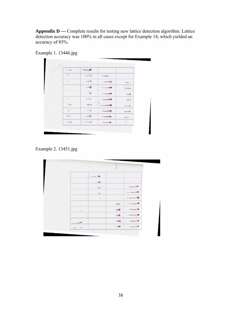
Appendix D — Complete results for testing new lattice detection algorithm. Lattice detection accuracy was 100% in all cases except for Example 14, which yielded an accuracy of 85%. Example 1. 13446.jpg
Example 2. 13451.jpg
38

Example 3. 13455.jpg
Example 4. 13460.jpg
39

Example 5. 13496.jpg
Example 6. 13497.jpg
40

Example 7. 13498.jpg
Example 8. 13499.jpg
41
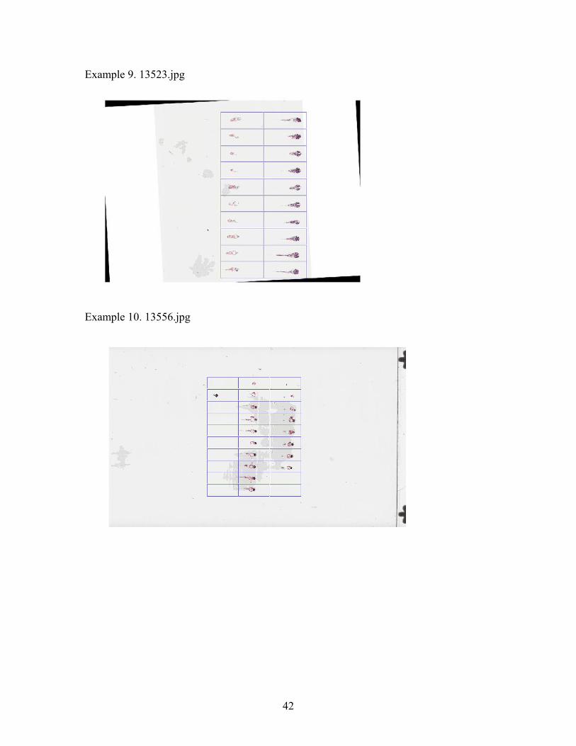
Example 9. 13523.jpg
Example 10. 13556.jpg
42
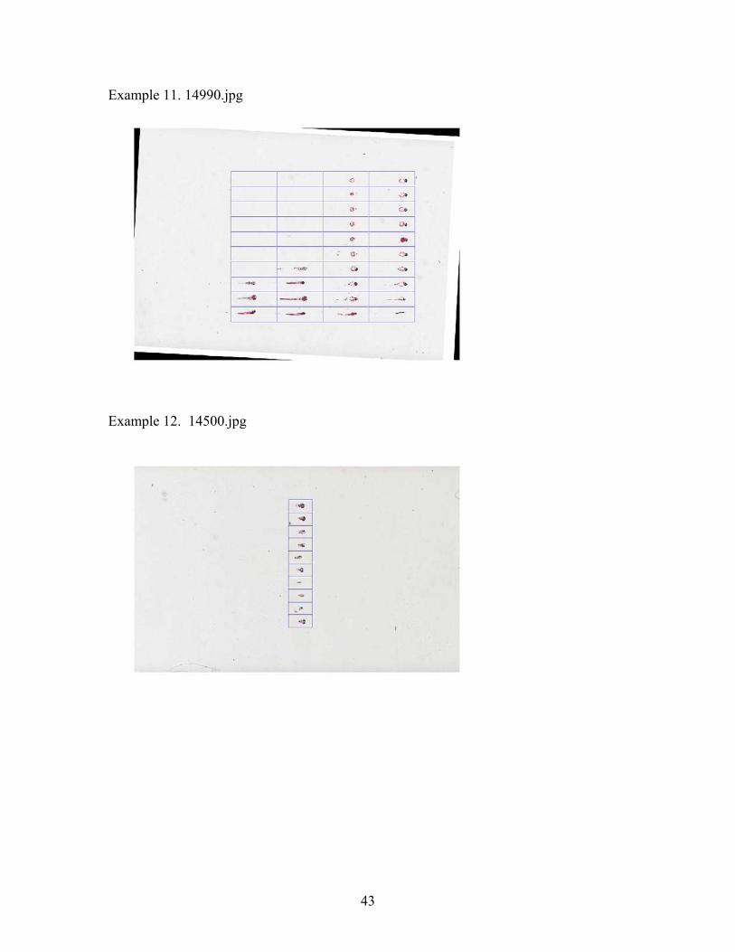
Example 11. 14990.jpg
Example 12. 14500.jpg
43

Example 13. 14510.jpg
Example 14. 14520.jpg
Here, the lattice detection accuracy is, at worst, 85% (28 out of 33 images correctly placed), although each specimen does lie within its own cell boundary. This lone suboptimal result is likely due to distortions that result from improper handling and sectioning of the tissue block.
44
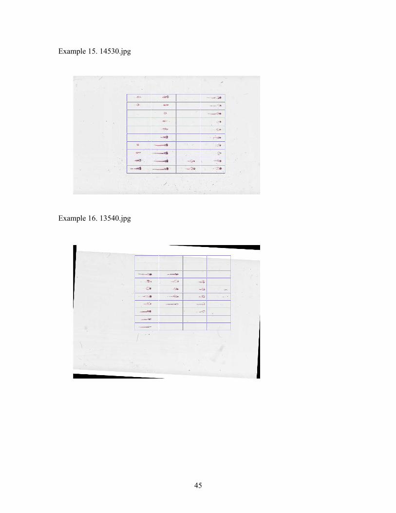
Example 15. 14530.jpg
Example 16. 13540.jpg
45
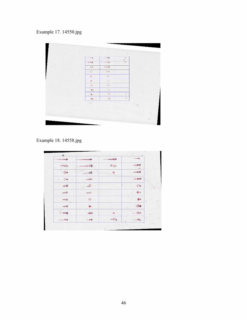
Example 17. 14550.jpg
Example 18. 14558.jpg
46

Example 19. 14595.jpg
Example 20. 14613.jpg
47