a computational comparison of symmetry handling methods ... · a computational comparison of...
TRANSCRIPT

A COMPUTATIONAL COMPARISON OF SYMMETRY HANDLINGMETHODS FOR MIXED INTEGER PROGRAMS
MARC E. PFETSCH AND THOMAS REHN
Abstract. The handling of symmetries in mixed integer programs in order to
speed up the solution process of branch-and-cut solvers has recently received
signi�cant attention, both in theory and practice. This paper compares di�erent
methods for handling symmetries using a common implementation framework.
We start by investigating the computation of symmetries and analyze the sym-
metries present in the MIPLIB 2010 instances. It turns out that many instances
are a�ected by symmetry and most symmetry groups contain full symmetric
groups as factors. We then present (variants of) six symmetry handling meth-
ods from the literature. Their implementation is tested on several testsets. On
very symmetric instances used previously in the literature, it is essential to use
methods like isomorphism pruning, orbital �xing, or orbital branching. More-
over, tests on the MIPLIB instances show that isomorphism pruning, orbital
�xing, or adding symmetry breaking inequalities allow to speed-up the solu-
tion process by about 15% and more instances can be solved within the time
limit.
Symmetries in mixed-integer programs (MIPs) have been known to slow down
branch-and-cut algorithms for a long time. The reason is that possibly many sym-
metric solutions appear in the branch-and-bound tree, although a single represen-
tative contains all essential information. Depending on the symmetry group, this
signi�cantly blows up the size of the branch-and-bound tree. During recent years,
several approaches to deal with this problem have been developed. Historically
the �rst approach is to add symmetry breaking inequalities or to perturb the ob-
jective function, which are folklore knowledge, see Sherali and Cole Smith [50]
and Ghoniem and Sherali [16] for recent examples. The handling of symmetries
in the tree received more attention in mathematical programming beginning with
“isomorphism pruning” by Margot [29, 30, 31, 32]. Subsequent developments are,
for example, “orbital branching” by Ostrowski et al. [37, 38] and generalized in-
vestigations by Liberti [27]. We refer to Margot [33] for a nice comprehensive
overview.
Moreover, symmetry handling techniques have found their way into commer-
cial solvers, like CPLEX, GUROBI, and XPRESS. Although the approaches used
in these solvers are not documented, it seems likely that they are based on tech-
niques similar to orbital branching, often combined with specialized symmetry
detection methods.
Nevertheless, as far as we know, there is no computational comparison of the
di�erent techniques and their strengths and weaknesses. One goal of this paper
is to close this gap. We present implementations of several techniques available
Date: November 2015.
2010 Mathematics Subject Classi�cation. 90C11,90C57.
Key words and phrases. symmetry, mixed-integer program, branch-and-cut, ismorphism prun-
ing, orbital branching.
1

A COMPUTATIONAL COMPARISON OF SYMMETRY HANDLING METHODS FOR MIPS 2
in the literature using the branch-and-cut framework SCIP [2, 48]. The imple-
mentation is publicly available through the web page of the �rst author and rests
on PermLib [42], a C++-library of the second author, for the necessary compu-
tations with permutation groups. (We note that the implementation for isomor-
phism pruning of Margot is available on his web page, as well.) Additionally, we
present several modi�cations and some new contributions for existing symmetry
handling methods.
Our paper is structured as follows. In Section 1, we de�ne symmetries of MIPs
and introduce necessary notation. Section 1.1 deals with the computation of sym-
metry groups. It seems to be folklore knowledge that this can be reduced to the
computation of graph automorphisms, and we discuss two ways to construct the
corresponding graphs. In Section 2, we introduce the implemented symmetry
handling methods, most of which are available in the literature:
◦ Orbital Fixing (Section 2.1),
◦ Isomorphism Pruning (Section 2.2),
◦ Orbital Branching (Section 2.3),
◦ Orbit Probing (Section 2.5),
◦ Symmetry Breaking Inequalities (Section 2.6),
◦ Projection onto the Fixed Space (Section 2.7).
Note that this list contains large parts of the proposed methods from the literature.
However, it cannot be comprehensive. For example, methods to improve primal
heuristics as in Christophel et al. [9] have not been implemented.
The heart of this paper are the extensive computational experiments in Sec-
tion 5. We compare the presented approaches on large testsets, including the
instances of Margot, MIPLIB 2003, and MIPLIB 2010.
These experiments have two goals: The �rst goal is to evaluate the potential of
symmetry handling methods. To this end, we analyze the symmetry groups of the
MIPLIB 2010 testset, see Section 4 and the appendix. It turns out that symmetry
appears in (surprisingly) many instances. Of course, the sizes of the symmetry
groups and their degree vary from instance to instance. In any case, there are
instances in this testset with a very high degree of symmetry, i.e., the sizes of
the symmetry groups are huge and they a�ect many variables of the instances.
Moreover, it turns out that most factors of the symmetry groups are symmetric
groups. We conclude that for instances of the MIPLIB 2010 (or similar), existing
algorithms that are simpli�ed and tuned for the special case of symmetric groups
will most probably be very useful for an e�cient solving. On the other hand,
there are special (combinatorial) instances like the Margot instances with large
and very complicated symmetries. For such instances, any solver that does not
handle symmetries will not be successful and symmetry handling will require
more advanced techniques. It therefore might be that specialized techniques for
such specially structured groups will appear in the future.
The second goal is to compare the performance of the di�erent symmetry han-
dling approaches on di�erent testsets. It turns out that on the instances of Margot,
with their relatively complicated symmetry groups, isomorphism pruning, or-
bital �xing, and orbital branching are the fastest; without these methods the per-
formance decreases dramatically. For instances from the MIPLIB, isomorphism
pruning and orbital �xing allow a speed-up of around 14 % and solve more in-
stances. Moreover, the addition of symmetry breaking inequalities performs very

A COMPUTATIONAL COMPARISON OF SYMMETRY HANDLING METHODS FOR MIPS 3
well with a speed-up of about 15 %. This suggests that more research is needed
on such inequalities and their ability to improve the dual bounds. For more con-
clusions from these experiments, see Section 6.
1. Symmetries of Mixed Integer Optimization Problems
Consider a mixed integer program (MIP) in the following form:
max c>x
Ax ≤ b (1)
x ∈ Zp ×Rn−p,
where A ∈ Rm×n, b ∈ Rm, c ∈ Rn, and 0 ≤ p ≤ n denotes the number of
integer variables. We write P := {x ∈ Rn : Ax ≤ b} for the polyhedron and
X := P ∩ (Zp ×Rn−p) for the feasible region corresponding to the MIP (1).
A symmetry of (1) is a bijection f : Rn → Rn such that f(X) = X and
c>f(x) = c>x for every x ∈ X . Thus, f maps feasible solutions of (1) to feasi-
ble solutions with the same objective. The symmetries of (1) form the so-called
symmetry group. However, the de�nition of a symmetry explicitly is based on the
feasible region X , which is in general not e�ciently handable (it is NP-hard to
decide whether X = ∅).
In practice, one therefore often only considers permutations of variables that
leave the descriptionAx ≤ b and the objective function c invariant, see, e.g., Mar-
got [33]. Here, the symmetric group, i.e., the set of all permutations on {1, . . . , n},is denoted by Sn, and a permutation π ∈ Sn acts on Rn by permuting the com-
ponents, i.e., π(x) := (xπ−1(1), . . . , xπ−1(n))>
for x ∈ Rn.
De�nition 1. A permutation π ∈ Sn of variables is a formulation symmetry of (1)
if there exists a permutation σ ∈ Sm such that
◦ π({1, . . . , p}) = {1, . . . , p} (i.e., π preserves integer variables),
◦ π(c) = c,◦ σ(b) = b, and
◦ Aσ(i),π(j) = Aij .
Thus, the rows of A are permuted by σ and the columns by π.
Remark 2. The above de�nition could be generalized in several di�erent ways.
First, one can consider permutations that leave P (instead of its formulation), the
integer variables, and the objective invariant, see, e.g., Bödi et al. [7]. Such sym-
metries can in principle be computed by normalization of the description ofP and
using graph automorphisms, see Herr [17]. This would avoid the e�ect that redun-
dant inequalities might change the symmetries of De�nition 1. To some extent,
one can take care of this aspect by computing the symmetries after preprocessing,
which performs a normalization and removes some redundant constraints.
A further generalization can be obtained by considering general linear bijec-
tion f with f(P ) = P that also preserve integrality of integer coordinates and
the objective function. Thus, one is interested in maps from GLp(Z)×GLn−p(R)that preserveP and do not change the value of the objective function, see Bremner
et al. [8], Bödi et al. [7], Herr [17], and Padberg [39]. If all variables are integral,
one extension is to consider subgroups of On(Z), so-called signed permutations,
see [7]. However, systematically computing GLp(Z)-symmetries of polyhedra is

A COMPUTATIONAL COMPARISON OF SYMMETRY HANDLING METHODS FOR MIPS 4
di�cult, see [8]. Moreover, two di�erent polyhedra yield the same setX , but have
di�erent symmetries because the feasible region is only a subset of the polyhedra.
As it is customary in many articles in mixed-integer programming, we will
exclusively deal with formulation symmetries as in De�nition 1 and therefore
simply refer to them as symmetries of (1) from now on. The group of all symme-
tries is the symmetry group G of (1) and is a subgroup of Sn, which we denote by
G ≤ Sn. The symmetry group can be (e�ciently) computed in practice and can
be represented via generators. We will discuss this in the next section.
1.1. Computing Symmetry Groups
Computing the symmetry group of a MIP is usually reduced to the determina-
tion of graph automorphisms, see Margot [33]. While the �rst (correct) approach
seems to be due to Salvagnin [44], many authors have (re)discovered this fact, see,
e.g., [6], Liberti [27], and Bödi et al. [7]. In the constraint programming literature,
a similar idea already appears in Puget [40].
The computational complexity of the graph automorphisms problem is still un-
known (it is neither known to be NP-hard, nor known to be solvable in polynomial
time), see, e.g., Read and Corneil [41] and Johnson [20]. There are, however, sev-
eral software tools which compute graph automorphisms e�ciently in practice
even for large graphs, e.g., nauty [34], saucy [10], and bliss [21].
A natural way to model MIP symmetries as graph automorphisms is via the
following bipartite graph (V ∪̇V ′, E) with vertex and edge colors. The set V ={v1, . . . , vn} contains a vertex vj for each variable xj of the problem; vj is col-
ored according to the objective coe�cient cj of variable xj . The second set V ′ ={v′1, . . . , v′m} contains a vertex for each linear inequality in Ax ≤ b. Each ver-
tex v′i is colored with respect to the coe�cient bi of the right-hand side. There
is an edge {v′i, vj} ∈ E if Aij 6= 0, and it is colored by the coe�cient Aij of
variable xj in the i-th constraint. Moreover, vertices v1, . . . , vp, corresponding to
integer variables, receive distinct colors from vp+1, . . . , vn. A graph automorphism
for this bipartite graph is now given by two bijections π : V → V , σ : V ′ → V ′
such that {σ(v′), π(v)} ∈ E if and only if {v′, v} ∈ E. It is easy to see that a
graph automorphism that respects the vertex and edge colors corresponds to a
symmetry according to De�nition 1 and conversely.
Note that 0-coe�cients play a special role in this construction. Of course, we
can replace 0 by any other number. However, the matrices appearing in MIPs are
often sparse. In this case, the choice of 0 as special coe�cient reduces the number
of edges in the graph and speeds up the symmetry computation.
The above mentioned graph automorphism software packages can only handle
vertex colors, but not edge colors. In fact, edge colors are not needed ifA contains
only one coe�cient di�erent from 0, e.g., if A is a 0/1-matrix. In the other cases,
one can reduce the problem to a purely vertex-colored instance by applying two
techniques that we describe in the following.
Salvagnin [44] discusses a transformation in which every edge {v′, v} ∈ Eis replaced by two edges {v′, w}, {w, v}, using an intermediate vertex w that is
colored with the original edge color.
Additionally, the number of newly introduced vertices can often be substan-
tially reduced by an idea of Puget [40]: Instead of adding new intermediate ver-
tices for all edges, vertices with the same color can be combined. For each v′i ∈ V ′

A COMPUTATIONAL COMPARISON OF SYMMETRY HANDLING METHODS FOR MIPS 5
A =
0 11 02 2
b =
112
c =
(11
)
1
2
3
x1
x2
1
2
3
x1
x2
A12
A21
A31/A32
1′
1
2′
2
3′
3
x′1x1
x′2x2
edge-colored matrix graph layered graph
Figure 1. Example for the reduction of symmetry computation with respect to (A, b, c) to graph
automorphisms.
let Vi,c ⊆ V be the set of vertices which are incident to v′i with an edge of color c.Then it is enough to introduce one intermediate c-colored vertex w with edges
to v′i and to all elements of Vi,c. We call this construction grouping by variables.In many MIP-instances, each constraint contains only few distinct variable coe�-
cients. In this case, the sets Vi,c are large, and the number of vertices in the graph
is signi�cantly reduced.
Depending on the distribution of coe�cients, it may be bene�cial to swap the
roles of constraints and variables to add as few intermediate vertices as possible.
For instance, if there are much more constraints than variables, it may help to add
one intermediate vertex between each vi and the set V ′i,c ⊆ V ′ of all “constraint”
vertices connected to vi by an edge of color c. We call this construction groupingby constraints. Because our original graph is bipartite, both groupings are possible.
In the following we will refer to either of these constructions as matrix graph; see
Figure 1 for an example.
The second, fundamentally di�erent transformation, is described in the man-
ual of the software nauty (version 2.4). Since it does not depend on bipartiteness,
we describe it for a general edge-colored graph (V,E). Let C be the total number
of distinct edge colors in this graph, and let L = dlog2(C + 1)e be the number of
bits needed to represent C . We introduce new vertex colors C1, . . . , CL and re-
place each vertex v ∈ V by vertices v1, . . . , vL that are colored with C1, . . . , CL,
respectively. Additionally, we add edges {v1, v2}, {v2, v3}, . . . , {vL−1, vL}. For
each edge {v, w} ∈ E with color c ∈ {1, . . . , C} of the original graph, we add
edges between vi andwi for each i-th bit that is 1 in the binary representation of c.Thus, we emulate the edge colors by vertex bit colors. Note that this transforma-
tion is described for a complete input graph. If the input graph is not complete,
we can augment it to a complete graph without loss of generality by adding the
missing edges with a new color which is not used in the input graph. We will refer
to this construction as a whole as as layered graph; see Figure 1 for an example.
The matrix graph hasm+n+O(N) vertices, whereN is the number of nonze-
ros in A. Depending on the distribution of di�erent coe�cients in the constraint
matrix, the last part may be much smaller than N . The layered graph results in
about (n+m) log2(C) vertices, whereC is the total number of distinct coe�cients
in the constraint matrix. Depending on the instance, either transformation might

A COMPUTATIONAL COMPARISON OF SYMMETRY HANDLING METHODS FOR MIPS 6
lead to a smaller graph. Thus, no construction dominates the other, in general.
We report on experience with graph sizes for practical instances in Section 4.
In any symmetry computation it is important to take numerical issues into ac-
count. For a very simple example, consider three matrix coe�cients α, β, γ, such
that α and β as well as β and γ are numerically equal (e.g., |α− β| ≤ ε and
|β − γ| ≤ ε, for some tolerance ε), but α and γ are not equal. Thus, the loss
of transitivity has to be taken into account in order to avoid wrong symmetry
computations. One method, also used by Salvagnin [45], is to �rst sort all coef-
�cients, say of A, non-decreasingly. Then passing through the sorted list, a new
color for Aij is used whenever |Aij − δ| > ε, where δ is the minimal coe�cient
belonging to the last used color. In this way, we have a stable behavior, but might
consider two coe�cients as di�erent that are still numerically equal. Thus, we
might compute a subgroup of the “real” symmetry group.
1.2. Permutation Groups
As mentioned earlier, the symmetry group of a MIP is a permutation group, i.e.,
a subgroup of the (full) symmetric group Sn. In this section we brie�y discuss
important structural aspects of permutation groups.
The degree of a permutation group is the number of moved points. If a per-
mutation group G is a direct product G = H1 × · · · ×Hk of some permutation
groups H1, . . . , Hk, it su�ces to consider each factor Hi independently, since the
groups H1, . . . , Hk act on disjoint sets of elements. In the following, we consider
single factors only.
As we will see later, for some symmetry handling techniques it is not enough
to know the abstract isomorphism type of a group, the action on the elements
is important as well. The most important case is that of groups isomorphic to
symmetric groups, which we will describe next.
LetG ≤ Sn be a permutation group of degree n, and letG ∼= Sm be isomorphic
to a symmetric group of degree m ≤ n. If m = n, we call the action of G a
coordinate action (that is, G is a natural representation of Sn). In the case m < n,
there may exist a group H ≤ Sm such that G is isomorphic to the particular
form {(π, π) : π ∈ H}; this of course means that H ∼= G ∼= Sm. We say that
such a group G has a matrix action (or is a diagonal group). Similar de�nitions
for coordinate and matrix actions can also be made for cyclic groups. Coordinate
and matrix actions of symmetric groups are especially nice from a computational
perspective. Their corresponding orbits, stabilizers, and minimal orbit elements
can be computed very fast in these representations.
Example 3. Some computations show that the groups
G1 = 〈(1 2 3 4 5 6), (1 2)〉 ≤ S6,G2 = 〈(1 2 3 4 5 6)(7 8 9 10 11 12), (1 2)(7 8)〉 ≤ S12, and
G3 = 〈(1 4 8 6 3 10)(2 7 9), (1 5 3 4 7)(2 10 6 8 9)〉 ≤ S10are all isomorphic to the symmetric group S6 on six elements. Here, we use the
standard cycle notation (i1, i2, . . . , ik) to denote a permutation π ∈ Sn with
π(i1) = i2, π(i2) = i3, . . . , π(ik) = i1, and π(i) = i for all other indices i ∈{1, . . . , n} \ {i1, . . . , ik}. Moreover, we denote by 〈π1, . . . , π`〉 the (permutation)
group generated by permutations π1, . . . , π`.

A COMPUTATIONAL COMPARISON OF SYMMETRY HANDLING METHODS FOR MIPS 7
Nevertheless, as symmetry groups of integer programs,G1,G2, andG3 behave
di�erently. The group G1 is a coordinate action. Group G2, which has degree 12,
is a matrix action and corresponds to permutations of the columns of a 2 × 6matrix, where the elements of the ground set correspond to the entries of the
matrix as follows:
A =
(1 2 3 4 5 67 8 9 10 11 12
).
For the action of groups likeG3 there is in general no obvious and nice interpre-
tation. Such groups appear, for instance, as symmetry groups of many instances
from the testset Margot1, see Section 5.
2. Exploiting Symmetries in MIPs
In this section, we review some well-known and some less-known techniques
to handle symmetries in MIPs, as well as new variants of these. Almost all ap-
proaches are presented for the mixed 0/1 case, i.e., all integral variables x1, . . . , xpare restricted to have values 0 or 1. The few exceptions that work for general MIPs
are mentioned explicitly.
One important issue that we also treat in this section is the compatibility of the
symmetry breaking methods with other solver components. Clearly, using two
symmetry breaking methods that are not based on the same principle can lead to
cutting o� all optimal solutions and thus to wrong results. We will therefore be
careful not to mix di�erent symmetry breaking methods.
An important method in MIP-solvers is bound propagation, i.e., based on the
current bounds of variables, further bounds of variables can be strengthened. In
the 0/1-case, bound propagations yield �xings of variables to 0 or 1 in the current
node (see below for examples). We distinguish this from branching on variables,
i.e., new nodes in the tree have been created by changing the bounds of a single
variable. Note that this notation deviates from parts of the literature, e.g., the
articles by Margot [30, 33] and Ostrowski et al. [37, 38], where �xings are called
settings and branchings are called �xings.
It is important to note that the dynamic techniques explained in the follow-
ing are not correct anymore, if branching is not performed on variables, e.g., by
branching on constraints. Moreover, components performing bound propaga-
tions/�xings have to be symmetry independent (this is called “strict setting algo-
rithm working under symmetry” by Margot [30]), i.e., they have to respect sym-
metry in the following sense: if the method is able to �x variable xi, it is (in prin-
ciple) also able to �x variable xπ(i) for all symmetries π. Of course, it may happen
in practice that not all �xings have been carried out, because of performance (e.g.,
iteration) limits in the implementation.
Most components of current MIP-solvers are symmetry independent, in par-
ticular, bound strengthening of linear constraints, dual reductions, reduced cost
strengthening etc. One symmetry independent operation that is typically subject
to performance limits is probing (see, e.g. Savelsbergh [47] and Achterberg [1]).
Furthermore, cutting planes that are valid for the convex hull of all feasible solu-
tions are symmetry independent, i.e., can be applied without con�ict with symme-
try handling methods. This includes all basic cutting planes like Gomory (mixed
integer) cuts or knapsack based cuts. We refer the reader to Margot [33, Sec-
tion 9.1.1] for a more elaborate discussion.

A COMPUTATIONAL COMPARISON OF SYMMETRY HANDLING METHODS FOR MIPS 8
Algorithm 1: Orbital Fixing
Input: G: symmetry group;
B0, B1: binary variables branched on 0/1 resp.;
F0, F1: binary variables �xed to 0/1 resp.
Output: L0, L1: binary variables that can be �xed to 0/1 resp.
1 compute Stab(G,B1) and its orbits O;
2 remove O ∈ O if O ∩B1 6= ∅ or O ∩ (V \B) 6= ∅;
3 L0 ← ∅, L1 ← ∅;
4 foreach orbit O ∈ O with |O| ≥ 2 do5 if O ∩ (B0 ∪ F0) 6= ∅ then6 L0 ← L0 ∪ (O \ (B0 ∪ F0));
7 if O ∩ F1 6= ∅ then8 L1 ← L1 ∪ (O \ F1);
In the following, let V := {1, . . . , n} be the indices of all variables and B :={1, . . . , p} ⊆ V be the indices of all binary variables. Then Stab(G,S) denotes
the stabilizer of the symmetry groupGwith respect to a subset S ⊆ V of variable
indices, i.e.,
Stab(G,S) := {π ∈ G : π(S) = S}.Moreover, the orbit of variable index i ∈ V with respect to G is O(i) := {π(i) :π ∈ G}. It is well known that the orbits partition the ground set V . For more
information about group theory, see, e.g., Lang [25].
Moreover, for the current node in a branch-and-bound tree, let B0, B1 ⊆ B be
the indices of binary variables that have been branched on 0 and 1, respectively,
and let F0, F1 ⊆ B be the indices of binary variables �xed to 0 and 1, respectively,
by some symmetry independent method or a single symmetry handling method.
We will assume that the setsB0,B1, F0, andF1 are pairwise distinct; in particular,
the current node is not trivially infeasible.
2.1. Orbital Fixing
A basic method to exploit symmetries in order to �x variables is orbital �xing,
which was introduced by Margot in [30, Sect. 4] and is described in Algorithm 1.
In order to argue the correctness of orbital �xing, we �rst note that Step 1 of
Algorithm 1 computes the orbital partition with respect to Stab(G,B1). Thus,
every such orbit that contains a variable in B1 only contains variables in B1.
Moreover, the variable types in each orbit are the same. Thus, orbits containing a
non-binary variable can be ignored for orbital �xing, which explains Step 2.
We cite the following result collected from the literature:
Lemma 4. Let F0 and F1 be obtained by symmetry independent methods, and letObe an orbit of Stab(G,B1).
◦ If O ∩ (B0 ∪ F0) 6= ∅ then all variables in O \ (B0 ∪ F0) can be �xed to 0.◦ If O ∩ F1 6= ∅ then all variables in O \ F1 can be �xed to 1.
This result was �rst obtained by Margot [30, Corollary 2] for a ranked branch-
ing rule. The restriction on the particular branching rule can be removed, as ob-
served by Ostrowski [36]. For the �rst part, see also Ostrowski et al. [38, Theo-
rem 3]. By this lemma, Steps 6 and 8 are correct.

A COMPUTATIONAL COMPARISON OF SYMMETRY HANDLING METHODS FOR MIPS 9
Algorithm 2: Isomorphism Pruning
Input: G: symmetry group;
B0, B1: binary variables branched on 0/1 resp.;
F0, F1: binary variables �xed to 0/1 resp.
Output: L0, L1: binary variables that can be �xed to 0/1 resp. or “cut o�”
1 if B1 = ∅ then2 compute sets L0 and L1 by orbital �xing w.r.t. B0, B1, F0, F1;
3 else4 if B1 is not a lexicographic representative then5 cut o� current node;
6 compute sets L0 and L1 by orbital �xing w.r.t. B0, B1, F0, F1;
Note that since O ∩ B1 = ∅ after Step 2, the variables in B1 are not relevant
in the second case. Moreover, by skipping orbits O that contain continuous vari-
ables, orbital �xing can be applied to mixed 0/1 problems (see Remark 5 below).
2.2. Isomorphism Pruning
Isomorphism pruning was introduced by Margot in [29]. It modi�es the search tree
such that it contains exactly one element from every orbit of optimal solutions of
the original problem. In the following, we consider a generalization for binary
MIPs as described by Ostrowski [36], which allows to use isomorphism pruning
without restrictions on the branching order.
Consider a node in the tree other than the root node, and let D := (i1, . . . , id)be the sequence of binary variable indices that have been branched on, from the
root to the current node; thus, d ≥ 1 is the depth of the node. Let B1 ⊆ D be the
subset of variable indices that have been branched to 1. Let π ∈ Sn be an arbitrary
permutation with π(k) = ik for k = 1, . . . , d. Then we can prune the current
node, if the set {k ∈ {1, . . . , d} : ik ∈ B1} is not lexicographically minimal in
its orbit under the conjugated symmetry group Gπ := {π−1gπ : g ∈ G}. The
argument is that in this case a branching set symmetric toB1 is used in some other
node, which will lead to symmetric solutions. It thus su�ces to consider only one
such node, see Margot [33] and Ostrowski [36] for details. The combination of
isomorphism pruning with orbital �xing yields Algorithm 2.
Remark 5. Note that the presence of continuous variables does not in�uence the
above arguments: If we set the indices of continuous variables to be last in the
ordering on which the lexicographic comparison is based, they do not change the
behavior of isomorphism pruning. Because continuous variables might be moved
by the symmetries used for checking the lexicographical order, we have to guar-
antee, however, that no solutions are cut o� by using symmetries on continuous
variables, i.e., all other solver components have to be symmetry independent. This
allows to use isomorphism pruning for mixed 0/1-problems.
Remark 6. General integer variables can be handled in several ways. First, Mar-
got [32] generalized isomorphism pruning to general integer programs. Second, if
we make sure that the integer variables are branched on after all binary variables
are branched on, the above argument for continuous variables holds for general
integral variables as well. This would, however, restrict the applicable branching

A COMPUTATIONAL COMPARISON OF SYMMETRY HANDLING METHODS FOR MIPS 10
Algorithm 3: Orbital Branching
Input: G: symmetry group;
B0, B1: binary variables branched on 0/1 resp.;
F0, F1: binary variables �xed to 0/1 resp.
Output: two new branching nodes if possible
1 compute Stab(G,B1) and its orbits O;
2 compute sets L0 and L1 by orbital �xing w.r.t. B0, B1, F0, F1;
3 choose O ∈ O with |O| ≥ 2, O ∩ (V \B) = ∅, O ∩ L0 = ∅, O ∩ L1 = ∅;
4 if not such O exists return;
5 create two branching nodes: one with variables B1 ∪ {minO} branched to 1
and one with variables B0 ∪O branched to 0;
6 in both branches �x variables in L0 and L1 to 0 and 1, respectively;
rules. Third, one can use the subgroup of G that only moves binary and continu-
ous variables, which is done in our implementation.
The key for a successful implementation is a representation of the symmetry
group that allows to e�ciently decide the lexicographic test above. Margot [29]
describes how this can be done using bases and strong generating sets.
2.3. Orbital Branching
Orbital branching was introduced by Ostrowski et al. [37, 38]. The basic idea is
the following: For each orbit O of the symmetry group containing only binary
variables, the following disjunction is valid:∑j∈O
xj ≥ 1∨ ∑
j∈Oxj ≤ 0.
Because of symmetry this is equivalent to:
xj = 1 for j = minO∨
xj = 0 ∀ j ∈ O.
In other words, we can branch on an orbit by setting all variables to 0 in one child
node and setting the variable with smallest index in O to 1 in the second child
node. Ostrowski et al. proved that this results in a valid branching rule, see [38,
Thm. 1 and 2]. Moreover, orbital �xing can also be included, see [38, Thm. 3].
Let G be the “global” symmetry group of the MIP (corresponding to the root
node). Then the stabilizer Stab(G,B1) is a subgroup of the “local” symmetry
group H1, obtained by �xing all variables in B1 to 1 and recomputing the sym-
metry group, see [38, Thm. 4]. Moreover, H1 is a subgroup of the local symmetry
groupH obtained by �xing all variables inB0 andB1 to 0 and 1, respectively, and
recomputing the symmetry group, see [38, Thm. 5]. Furthermore, the latter result
also holds if orbital �xing is performed. Following [38], in our implementation
we perform the �xings already when creating the nodes. These arguments show
that Algorithm 3 is correct.
There are two degrees of freedom in the algorithm: The choice of the orbit and
of the symmetry group. For the symmetry group, we may either use the “global”
symmetry group Stab(G,B1) or the “local” symmetry group H , which may be

A COMPUTATIONAL COMPARISON OF SYMMETRY HANDLING METHODS FOR MIPS 11
larger than the global symmetry group. Following the experimental results of [38],
we use Stab(G,B1).
For the choice of the orbit to branch on, several rules were described and
tested in [38]; we only describe four rules here. For this we denote by G(O) :=Stab(G,B1 ∪ {minO}) the symmetry group after 1-branching on O.
◦ branch largest: choose orbit O for which |O| is maximal (Rule 1);
◦ branch break symmetry: choose orbit O for which |G(O)| is minimal (Rule 4);
◦ branch keep symmetry: choose orbit O for which |G(O)| is maximal (Rule 5);
◦ branch max product: choose orbit O for which
|O| ·max{|O′| : O′ orbit of G(O)}
is maximal (Rule 6).
We evaluate these di�erent settings in our computational experiments.
Remark 7. Note that again the presence of continuous variables does not in�u-
ence the validity of orbital branching as long as no solutions are cut o� by using
symmetries on continuous variables. Moreover, orbital branching can in principle
be extended to general bounded MIPs by an encoding with binary variables, but
it is then questionable to yield good performance.
2.4. Truncation Techniqes
Because group computations can be expensive, we might save time by skipping
dynamic symmetry exploiting techniques in the deeper parts of the branch-and-
bound tree. Besides using a static limit on the tree depth, another possibility is to
stop symmetry handling for all children of a node in which the computed sym-
metry group is trivial. As the following example shows, this is only a heuristic,
because symmetries might reappear in deeper levels of the tree.
Example 8. Consider the following MIP:
x1 + 2x2 + 3x3 + 4x4 ≤ 5,
2x1 + 3x2 + 4x3 + x4 ≤ 5,
3x1 + 4x2 + x3 + 2x4 ≤ 5,
4x1 + x2 + 2x3 + 3x4 ≤ 5,
x1, x2, x3, x4 ∈ Z.
The symmetry group is the cyclic groupC4 = 〈(1 2 3 4)〉. If we branch on x1 = 1,
then the corresponding node has only trivial symmetries. Branching further on
x3 = 1 yields the problem
2x2 + 4x4 ≤ 1,
3x2 + x4 ≤ −1,
4x2 + 2x4 ≤ 1,
x2 + 3x4 ≤ −1,
x2, x4 ∈ Z.
The symmetry group of this child problem is Stab(C4, {1, 3}) = 〈(1 3)(2 4)〉.Note that, in general, Stab(G,F1) is a proper subgroup of the symmetry group.

A COMPUTATIONAL COMPARISON OF SYMMETRY HANDLING METHODS FOR MIPS 12
Algorithm 4: Orbit Probing
Input: G: symmetry group
Output: L0, L1: binary variables �xed to 0/1 resp.
1 L0 ← ∅, L1 ← ∅;
2 repeat3 compute H = Stab(Stab(G,L1), L0);
4 compute orbits O of H ;
5 foreach orbit O with |O| ≥ 2, O ∩ (L0 ∪ L1) = ∅ do6 let k = minO be the �rst variable in O;
7 �x all variables in O to 0 and perform constraint propagation;
8 if infeasible then9 L1 ← L1 ∪ {k} (�x variable k to 1);
10 �x variable k to 1 and perform constraint propagation;
11 if infeasible then12 L0 ← L0 ∪O (�x all variables in O to 0);
13 Let S0 and S1 be the variables outside of O �xed to 0 and 1,
respectively, by both constraint propagations;
14 L0 ← L0 ∪ S0, L1 ← L1 ∪ S1;
15 if �xings found then16 break for loop;
17 until no �xings are found;
2.5. Orbit Probing
Probing for mixed 0/1-problems refers to the following method (see, e.g., Savels-
bergh [47] and Atamtürk et al. [4]): Each binary variable is tentatively �xed to 0and 1, respectively. In each case, a propagation round is performed, i.e., it is
checked whether additional variables can be �xed. If infeasibility is detected in
either case, one can �x the variable to the opposite value. (If both cases are infea-
sible, the whole instance is infeasible.) If some other non-�xed variable is �xed
to the same value in either branch, one can �x it to this value. Moreover, this
method allows to detect implications between variables that can later be used to
derive additional inequalities. Probing is often successful for 0/1-variables that
are e�ected by symmetry if symmetry handling is performed by any method that
allows to �x variables.
Moreover, combining the ideas of orbital branching and probing, one obtains
orbit probing, which seems to be a new idea: All variables in an orbit are tentatively
�xed to 0. If the resulting problem is infeasible, one may �x the �rst variable in
the orbit to 1. Otherwise, the �rst variable in an orbit is tentatively �xed to 1. If
this is infeasible, one may �x all variables in the orbit to 0. Moreover, one may
�x variables outside the orbit, if they have been �xed to the same values in both
cases. This leads to Algorithm 4, which is correct due to the correctness of orbital
branching. Note that we recompute the stabilizer of the group and its orbits after
each �xing.
A COMPUTATIONAL COMPARISON OF SYMMETRY HANDLING METHODS FOR MIPS 13
2.6. Symmetry Breaking Ineqalities
Another way to use symmetry in discrete optimization is to add inequalities to
tighten the search space. Many examples appear in the literature, see, for example
Sherali and Cole Smith [50] and Margot [33] for an overview.
In the case of a general MIP with symmetry group G, the goal is to modify
the feasible region in such a way that it is contained in a fundamental domainforG, see Friedman [13]. A fundamental domain is a polyhedron containing only
one element from each G-orbit (this de�nition can be generalized to arbitrary re-
gions, see Margot [33]). Therefore, the branch-and-bound tree does not encounter
symmetric (optimal) solutions twice. In general, for any d ∈ Rn, one can add in-
equalities
d>x ≤ d>π(x) (2)
for each element π ∈ G. For instance, taking d = (2n−1, 2n−2, . . . , 2, 1)> leads
to a lexicographic ordering if x is binary and produces a minimal fundamental
domain, as proved by Friedman [13]. However, tight IP formulations for funda-
mental domains are in general hard to obtain or not practical, because of their size
and of numerical problems in the description if the above lexicographic ordering
is used. For the special cases of coordinate actions of the symmetric group and
cyclic group, Friedman discusses e�cient separation algorithms.
For a cyclic group Ck acting on variables x1, . . . , xk the following give valid
inequalities, which seem to be part of the folklore (see, e.g., Liberti[26, 27]):
x1 ≤ x2, x1 ≤ x3, . . . , x1 ≤ xk. (3)
If a symmetric group Sk acts on the variables x1, . . . , xk, a tight IP formulation is
given by
x1 ≤ x2 ≤ · · · ≤ xk. (4)
In fact, if all variables x1, . . . , xk are integral, [18] showed that
xk ≤ x1 + 1 (5)
is a valid inequality for the symmetric group case. For matrix actions of cyclic
or symmetric groups, Inequalities (3) and (4) remain valid when restricted to a
single row. However, the additional inequality (5) cannot be generalized to matrix
actions (see [43, Sec 6.2.2]).
For general groups, one can use Inequalities (2). In order to obtain numerically
more stable inequalities, we use d = (1, 2, 3, . . . , n)>, i.e.,
x1 + 2x2 + · · ·+ k xk ≤ xπ(1) + 2xπ(2) + · · ·+ k xπ(k). (6)
To control the size, we only add these inequalities for the generators of G.
Liberti [27] discusses the possibility of adding inequalities that amount to se-
lecting an arbitrary element of each orbit and adding inequalities like (3) to ensure
that this variable is the smallest. Approximations of fundamental domains, i.e.,
symmetry breaking inequalities were for example described by Liberti [26].
For cyclic or symmetric groups acting on columns of 0/1-matrices with addi-
tional partitioning or packing conditions on the rows, so-called orbitopes can be
used to completely handle symmetries. On the one hand, a complete linear de-
scription is known, see [23] and also Faenza and Kaibel for a shorter proof [11].
On the other hand, a method (orbitopal �xing) to further �x variables based on all
currently branched or �xed variables has been introduced in [22] and was shown

A COMPUTATIONAL COMPARISON OF SYMMETRY HANDLING METHODS FOR MIPS 14
to be slightly faster than the separation of inequalities. Thus, we use orbitopal
�xing by default.
We generally have to be careful not to add con�icting symmetry breaking in-
equalities. In our implementation we ensure this by adding only one type of in-
equality for each component of the direct product. See Liberti [27] and Liberti
and Ostrowski [28] for alternative approaches.
Note that all techniques explained in this section (with the exception of or-
bitopes), i.e., inequalities (3), (4), and (6), work for general MIPs; Inequality (5) is
valid for integral variables.
2.7. Projection onto the Fixed Space
While all previously mentioned methods need binary (or integral) variables, the
following result allows to �x continuous variables to be equal within orbits. We
call a symmetry continuous variable restricted (CVR) if it �xes all binary and integer
variables pointwise.
Lemma 9. Let the MIP (1) be feasible and letG′ be the subgroup of CVR symmetries.Then there exists an optimal solution x̄with x̄i = x̄j for all i, j ∈ O and for all orbitsO of continuous variables with respect to G′.
Proof. Let x? be an optimal solution of the MIP (1), and de�ne
x̄ =1
|G′|∑π∈G′
π(x?).
By assumption, π(i) = i for all π ∈ G′ and all integer variable indices i ∈{1, . . . , p}. Thus, x̄i = x?i for all i = 1, . . . , p. Since (1) is convex with respect to
the continuous variables and each π(x?) is feasible, x̄ is feasible for (1). Moreover,
we have
c>x̄ =1
|G′|∑π∈G′
c>π(x?)︸ ︷︷ ︸=c>x?
= c>x?.
Thus, x̄ is optimal as well. We have for any σ ∈ G′:
σ(x̄) =1
|G′|∑π∈G′
σ(π(x?)) =1
|G′|∑γ∈G′
γ(x?) = x̄,
since there is a bijection between each γ ∈ G′ and σ ◦ π for π = σ−1 ◦ γ ∈ G′.Consequently, x̄ is constant along each orbit, which shows the claim. �
The core idea of this lemma has been known for more general convex programs
for some time; see, for instance, Gatermann and Parrilo [15, Thm. 3.3] in the
context of semide�nite programs. An extension to integer programs is “orbital
shrinking” by Fischetti and Liberti [12] (see also Salvagnin [46] and Mittelmann
and Salvagnin [35] for applications).
Remark 10. The above proof implicitly refers to the �xed space of the group:
Fix(G) = {x ∈ Rn : x = π(x) for all π ∈ G}.In fact, setting the variables to be equal within orbits corresponds to a projection
on the �xed space. Using the �xed space for integer programming is discussed
by Bödi et al. [7] and in [18]; see also [17, 19, 43]. For highly symmetric prob-
lems – the symmetry group is the alternating or symmetric group – this yields a

A COMPUTATIONAL COMPARISON OF SYMMETRY HANDLING METHODS FOR MIPS 15
polynomial-time algorithm to solve IPs [7]. More generally, knowledge of lattice-
free orbit polytopes may allow to restrict IPs to integer points close to the �xed
space, which improves the performance of MIP solvers in some cases, see [18].
Remark 11. If we also allow non-CVR symmetries, i.e., we have a group act-
ing on both continuous and integer variables, optimal solutions can be cut o� by
projection onto the �xed space as the following example shows:
max x4 + x5 + x6
2x4 + 3x5 + x1 + x2 ≤ 3,
2x5 + 3x6 + x2 + x3 ≤ 3,
2x6 + 3x4 + x3 + x1 ≤ 3,
x1 + x2 + x3 ≥ 1,
x1, x2, x3 ∈ Z+.
The symmetry group is a cyclic group generated by (1 2 3)(4 5 6). An optimal
solution is given by (1, 0, 0, 835 ,
1835 ,
2335)>. However, no point with x4 = x5 =
x6 = 715 = 1
3 ·4935 is feasible.
3. Implementation Details
We implemented the methods described in Section 2 in C++ using SCIP [48] ver-
sion 3.2 with CPLEX 12.6.1 as LP solver. The symmetry computations are per-
formed through PermLib, a C++ library for symmetry computations with permuta-
tions written by the second author [42]. The graph automorphisms are computed
using bliss 0.72 [21].
We provide some details on the implementation:
Symmetry Detection. Symmetry can be determined before or after presolving.
Presolving can on the one hand remove symmetry, e.g., if variables are aggregated,
or it can produce symmetry, e.g., if variables are eliminated that previously were
the source of non-symmetry. If symmetry is detected before presolving, one needs
to be careful that no successive presolving step destroys the found symmetry. In
this case, we turn o� presolving steps that can break symmetries. In SCIP this
refers to the gateextraction, dominated column, and component presolvers. In any
case, we make sure that symmetry is computed only once and only if it is required.
Moreover, we make sure that certain types of variables are �xed pointwise, if this
is needed. Furthermore, in order to avoid overly large computation times in this
component, we limit the number of produced generators to 1500.
Heuristic for Symmetric Subgroups. We also implemented a fast heuristic that
recognizes symmetric groups from transpositions. The resulting subgroup of the
symmetry group is either trivial or is a direct product of coordinate actions of
symmetric groups. This heuristic should be faster for detecting symmetry and for
computing stabilizers or lexicographic representatives.
IsomorphismPruning. The implementation of isomorphism pruning only deals
with the mixed 0/1-case, since the general case is signi�cantly more complicated
to implement. Note, however, than an implementation (isop-1.2) of the general
integer case is available on the web page of Margot. Isomorphism Pruning is
always combined with orbital �xing in our implementation, and the truncation
techniques described in Section 2.4 can be applied.

A COMPUTATIONAL COMPARISON OF SYMMETRY HANDLING METHODS FOR MIPS 16
Orbital Branching. In the implementation of orbital branching, we also inte-
grate orbital �xing. The corresponding �xings are performed at the time of cre-
ating the branching nodes. We also allow for the truncation of orbital branching
in subnodes, see Section 2.4.
Orbital Fixing. Orbital �xing is also available as a separate propagation method
and can be truncated in subnodes, see Section 2.4.
Symmetry Breaking Inequalities. We �rst split the symmetry group into a di-
rect product so that each factor cannot be further decomposed. We then apply
the basic group recognition of PermLib and add individual symmetry-breaking
inequalities for each factor separately. If we detect a coordinate action of a cyclic
or symmetric group, we add the Inequalities (3) and (4) (as well as (5) for integer
variables), respectively. For matrix actions of cyclic or symmetric groups, we add
Inequalities (3) or (4) for the �rst orbit only. We also try to detect an orbitope
structure and apply the corresponding orbital �xing algorithm, see Section 2.6.
If none of the previous symmetry-breaking inequalities could be used, we allow
to add inequalities (6) for each generator of the group. Additionally probing can
be performed for all variables that are moved by a cyclic or symmetric group and
for the diagonal variables in possibly detected orbitope structures.
Orbit Probing. Orbit probing (see Section 2.5) is implemented straightforwardly,
where the most time consuming step is to recompute the stabilizer (H in Algo-
rithm 4). In order to limit the time resources, the default is to consider each vari-
able at most once (even if probing with a di�erent stabilizer group H might lead
to reductions later). After orbit probing, we replace the symmetry group by the
stabilizer of the variables �xed to 0 and 1 by orbit probing.
Fixed Space Projection. In the implementation, we take care to apply the pro-
jection only for the �xed space of the subgroup of CVR symmetries. The cor-
responding variables are aggregated to be equal, i.e., they are removed from the
problem.
PermLib. For all operations with permutation groups we use the second author’s
C++ library PermLib [42]. It o�ers basic functionality like orbit and stabilizer
computations similar to GAP [14]. It represents permutation groups by bases and
strong generating sets and employs backtrack search to compute set stabilizers
(see also [49]). In order to decide whether a set is lexicographically minimal we
implemented a backtrack search as described by Margot [30, Sec 6.2].
Computational Experiments. We performed extensive computational experi-
ments to evaluate the performance of the various symmetry handling methods.
The goal of the di�erent experiments is to answer the following questions:
◦ How symmetric are di�erent instances used in the literature?
◦ What kind of symmetries do appear?
◦ What is the proportion of time needed for computing symmetries?
◦ Can we reproduce computational experiments published in the literature?
◦ Depending on the instances, does it pay o� to use symmetry handling?
◦ Which symmetry handling method is the best?
All computations were performed on a Linux cluster with Intel i3 CPUs with
3.2Hz, 4MB cache, and 8GB memory running Linux. Each computation was per-
formed single-threaded and a single process running on each computer. The code
was compiled with gcc 4.4.5 with -O3 optimization.

A COMPUTATIONAL COMPARISON OF SYMMETRY HANDLING METHODS FOR MIPS 17
Table 1. MIPLIB 2003 instances with symmetry before and after presolving; listed is the number
of variables and constraints, the time to detect automorphisms of the graph as well as the total time
(including the preparation of data structures), and the number of generators.
before presolving after presolving
graph total total
name #vars #conss time time # gen #vars #conss time # gen
arki001 1388 1049 0.03 0.03 37 961 762 0.02 0
atlanta-ip 48,738 21,733 115.26 187.98 11,685 17,270 19,114 0.26 0
ds 67,732 657 0.28 0.30 2 64,030 626 0.28 0fast0507 63,009 508 1.13 3.69 828 20,676 441 0.04 0
�ber 1298 364 0.00 0.00 1 1043 290 0.01 0
glass4 322 397 0.00 0.00 1 317 393 0.00 1liu 1156 2179 0.01 0.01 1 1154 2179 0.01 0
mas74 151 14 0.00 0.00 2 150 14 0.00 2
mas76 151 13 0.01 0.01 2 150 13 0.00 2misc07 260 213 0.01 0.01 2 232 224 0.00 2
mkc 5325 3412 0.20 0.23 195 3273 1288 0.13 194mod011 10,958 4481 0.61 3.52 829 6489 1951 0.02 6
momentum3 13,532 56,823 1.04 1.07 55 13,151 49,376 0.90 0
msc98-ip 21,143 15,851 14.01 144.99 5151 12,725 14,988 0.13 4mzzv11 10,240 9500 0.12 0.16 155 6558 6410 0.04 1
mzzv42z 11,717 10,461 0.11 0.15 110 7480 7372 0.06 0
net12 14,115 14,022 0.09 0.09 0 12,523 12,768 0.08 4noswot 128 183 0.01 0.01 1 120 172 0.01 3
nsrand-ipx 6621 736 10.27 11.70 876 3798 536 0.04 1
nw04 87,482 37 27.00 110.48 4505 46,143 36 0.18 0opt1217 769 65 0.00 0.00 1 759 65 0.00 0
p2756 2756 756 0.01 0.01 29 2065 1422 0.02 25
protfold 1835 2113 0.02 0.02 2 1835 2113 0.02 2qiu 840 1193 0.01 0.01 4 840 1193 0.01 4
rout 556 292 0.00 0.00 4 555 291 0.00 4
seymour 1372 4945 0.03 0.05 216 912 4412 0.01 2stp3d 204,880 159,489 6.69 10.15 594 137,633 97,980 1.57 0
swath 6805 885 0.24 0.72 461 6260 483 0.01 0t1717 73,885 552 2565.42 2566.29 26,454 16,102 552 0.04 0
timtab1 397 172 0.00 0.00 1 201 167 0.00 1
timtab2 675 295 0.00 0.00 1 341 290 0.00 1
All times that we report are in seconds. The time limit for all computations has
been set to 1 hour. The time for instances that run into the time limit is evaluated
as 3600 seconds.
4. Computational Results for Computing Symmetries
The power of using symmetry handling methods depends on the amount and type
of symmetry present in the tackled instances. Thus, as a �rst step, we analyzed
the symmetry groups of MIPLIB instances.
4.1. MIPLIB 2003
For the MIPLIB 2003 [3], Table 1 shows the list of instances that contain symmetry
before and after presolving. Note that Liberti [27] determined the types of the
symmetry groups for these instances before presolving.
For instances containing symmetry, some additional work is necessary to trans-
form the computed graph automorphisms into the internal data structures of
PermLib. This explains the di�erence between “graph time”, i.e., the time needed

A COMPUTATIONAL COMPARISON OF SYMMETRY HANDLING METHODS FOR MIPS 18
Table 2. Times for MIPLIB 2010 (total # 331) symmetry detection split into instances with and
without symmetry: column “group” displays whether the full group is computed or the heuristic to
detect symmetric groups is used. Column “presol” shows whether presolving is turned on. Column
“graph time” and “total time” show the geometric means of the time in seconds to compute graph
automorphisms and to compute symmetry in total, respectively. Column “limits” gives the number
of instances for which symmetry computation failed because of the memory or time limit.
Parameters with symmmetry without symmetry
group graph presol # graph time total time # time #limits
full layered no 171 2.47 3.05 149 2.12 11
full matrix no 171 1.97 2.54 149 1.85 11
heur layered no 110 3.23 3.23 211 1.32 10
heur matrix no 115 3.44 3.45 211 1.18 5
full layered yes 153 1.61 1.67 178 1.33 0
full matrix yes 153 1.36 1.43 178 1.24 0
heur layered yes 53 1.58 1.58 278 1.28 0
heur matrix yes 53 1.47 1.48 278 1.16 0
by bliss, and the “total time”. Clearly, for instances without symmetry no addi-
tional work is necessary.
The results show that 30 of the 60 MIPLIB 2003 instances contain symmetry
before presolving. The number of generators varies between 1 and 26,454. Not
surprisingly, a larger number of generators typically leads to a larger time to com-
pute symmetry. The time needed to compute graph automorphisms is usually
small, with some extreme exceptions (e.g., t1717 before presolving). The addi-
tional time needed to set up the PermLib data structures is usually small as well,
but sometimes noticeable.
Moreover, 18 instances contain symmetry after presolving. Thus, presolving
generally reduces symmetry, as can also be seen by the often signi�cantly reduced
number of generators. One particular presolving step that reduces symmetry is
the elimination of parallel or dominated columns. However, note that sometimes
the number of generators increases (e.g., noswot) and there are instances in which
presolving introduces symmetry (e.g., net12). The time for symmetry computa-
tion after presolving is quite small.
4.2. MIPLIB 2010
We next report on the symmetries present in the MIPLIB 2010 [24] instances. The
testset for this section consists of all 361 problems in the MIPLIB 2010, excluding
the 21 “unstable” and 11 “XXL” instances. This leaves 331 instances (two instances
are contained in both subsets).
On these instances, we ran the two algorithms described in Section 1.1 to con-
struct the vertex-colored graphs whose automorphism group corresponds to the
symmetry group of the MIPs. As a heuristic for the decision of whether to group
by variables or by constraints in the matrix graph, we group by variables when-
ever there are more variables than constraints.
The results are given in Table 2. The lines are grouped by the fact whether the
“full” symmetry group is computed or whether the “heuristic” detection of sym-
metric coordinate subgroups is used (see Section 3). Moreover, either the “matrix”
or “layered” graph is used, and presolving is used or not. For some instances, we
ran into the time limit or the memory limit of 8 GB, which is accounted for in the
last column.
A COMPUTATIONAL COMPARISON OF SYMMETRY HANDLING METHODS FOR MIPS 19
The results show that there are at least 171 instances initially containing sym-
metry, but only 154 if presolving is used. Thus, as for the MIPLIB 2003 instances,
presolving already eliminates a certain amount of symmetry. If we use the heuris-
tic for symmetric coordinate subgroups, the numbers reduce to at least 115 before
and 53 after presolving, respectively. While the computation times of the heuris-
tic for instances with symmetry are larger on average, the times are reduced for
those instances that do not contain symmetry. Furthermore, the time needed for
computing symmetries by the matrix graph is faster on average. An exception
are the heuristic settings without presolving (data lines 3 and 4 in Table 2). How-
ever, here the matrix representation can compute �ve more instances within the
memory limit.
We then tried to analyze the symmetry group G using PermLib on a computer
with more memory (32 GB). The results are given in the Table 19 in the appendix.
There are 194 instances that might have a nontrivial symmetry group. The analy-
sis ran into the memory limit or time limit of 10 hours for 19 instances. Thus, there
are 175 instances for which we actually tried to analyze the symmetry group.
The size of the symmetry groups range from 2 to about 1041641.2. The percent-
age of variables that are moved by symmetry ranges from close to 0 % to 100 %.
In total 35,042 factors were analyzed, and they very often consist of coordinate
or matrix actions of some Sk: There are 29,962 and 4769 factors of coordinate
and matrix actions of symmetric groups, respectively. However, the coordinate
actions very often involve small symmetric groups. The type of about 294 factors
could not be identi�ed. No cyclic groups (other than S2) were detected.
Moreover, for 120 of the 331 examined MIPLIB2010 instances, in total 102,190coordinate actions of full symmetric groups were found by the heuristic that rec-
ognizes symmetric groups from transpositions; the computation was stopped be-
cause of the memory or time limit for only two instances. In fact, this method
�nds signi�cantly more symmetric group factors than the �rst analysis since it
is able to complete the computations also for highly symmetric instances. These
instances contribute the major share of symmetric group factors (see the table in
the online supplement).
If we analyze the groups after presolving the picture changes as follows (see
the table in the online supplement): 157 still contain symmetry, and we ran into
the memory limit for two instances. In total 10,505 factors were analyzed, 9662and 716 where coordinate and matrix actions of symmetric groups, respectively.
The type of 125 factors could not be identi�ed.
5. Computational Results for Symmetry Handling Methods
We use following testsets:
Margot1: instances used in [30] (total: 16); we complemented the STS instances
as described there.
Margot2: additional highly symmetric instances by Margot [32, 33], available on
the web page of François Margot (total: 79);
M2003-sym: all instances from MIPLIB 2003 [3] for which we found a non-trivial
symmetry group after presolving (total: 18).
M2010-sym: all instances from the MIPLIB 2010 [24] for which we found a non-
trivial symmetry group after presolving (total: 154);
M2010-bench: all instances from the MIPLIB 2010 benchmark suite (total: 87);

A COMPUTATIONAL COMPARISON OF SYMMETRY HANDLING METHODS FOR MIPS 20
In this section, we report on computational experiments that investigate the
di�erent symmetry handling methods on these testsets. One one hand, we study
di�erent settings for the same method and on the other hand compare the di�erent
strategies. As a basis of comparison, we take SCIP with default settings, labeled
as default.
For reporting aggregated results, we use the shifted geometric mean of values
t1, . . . , tn: (∏(ti + s)
)1/n − swith shift s. We use a shift s = 10 for time and s = 100 for branch-and-bound
nodes in order to decrease the strong in�uence of very easy instances in the mean
values, see Achterberg [1] for more information. In all tables below that report
aggregated results, #nodes refers to the shifted geometric mean of the number of
nodes in the branch-and-bound tree, time refers to the shifted geometric mean of
the CPU time in seconds. Note that all times for the symmetry handling methods
always include symmetry computation. Moreover, note that it depends on the
particular symmetry group and the types of the variables it acts on whether a
particular method allows to exploit symmetry.
The detailed results of all settings on all testsets are given in the extensive
online supplement, containing about 170 tables.
5.1. Experiment 1: Comparison to the Literature
To begin our computational evaluation of the implemented symmetry handling
methods, we compare the results of our implementation of isomorphism pruning
and orbital branching with results published in the literature. Clearly, since the
results have been obtained on di�erent computers and with di�erent branch-and-
cut frameworks, it cannot be expected that the running times are the same. We
would, however, expect the number of nodes to be roughly the same. Moreover,
symmetry handling should clearly turn out to be e�ective, since this is one of the
main results of the papers published in the literature.
Table 3 presents the best results from Margot [30] and Ostrowski et al. [38] on
the Margot1 testset and compares them to two variants of our implementation
that were able to solve all instances (see Section 5.2 and Section 5.3, respectively).
For isomorphism pruning, branching on the �rst index was used, as it was done
in [30]. Let us mention that the results get worse, if we use a di�erent branching
rule – compare the experiments in Section 5.2. Moreover, note that [38] does not
present results of orbital branching for some of the instances in the testset.
The results show that our implementation produces about the same number
of nodes as the implementations in the literature. Moreover, there seems to be
a slight tendency that isomorphism pruning produces less nodes than orbital
branching; but see Section 5.8 for the comparison of the timings.
5.2. Experiment 2: Isomorphism Pruning
We next compare di�erent versions of isomorphism pruning (ISP) (see Section 2.2):
ISP: isomorphism pruning with default SCIP branching rule;
ISP-heur: ISP with heuristic symmetry detection (see Section 3);
ISP-NST: ISP with “no subtree”: symmetry handling is turned o� in the subtree
of a node for which the stabilizer of the �xed variables is empty;

A COMPUTATIONAL COMPARISON OF SYMMETRY HANDLING METHODS FOR MIPS 21
Table 3. Comparison of the number of nodes in the B&B-tree used by di�erent implementations
of isomorphism pruning and orbital branching on the Margot1 testset: 1. isomorphism pruning
implementation of Margot [30] (Table 2, version BC2), 2. our implementation, 3. implementation
of orbital branching by Ostrowski et al. [38] (Table 3, Rule 5), and 4. our implementation.
isomorphism pruning orbital branching
Problem #nodes [30] #nodes ISP-�rst #nodes [38] #nodes OB-orbit3
cov954 655 287 249 79cov1053 681 572 9775 1027
cov1054 447 685 1249 15,884
cov1075 470 578 381 130cov1076 22,454 31,726 31,943 26,372
cov1174 69,036 158,549 — 227,356
cod83 79 22 25 43
cod83r 121 69 — 68
cod93 653 1884 1361 3030cod93r 1301 2181 — 3100
cod105 19 7 11 7
cod105r 13 5 — 5
sts45 1571 1820 4709 2284
sts63 4499 4203 5533 5550sts81 503 1149 6293 1217
ISP-first: isomorphism pruning with �rst index branching;
ISP-NST-first: ISP-NST with �rst index branching.
Table 4 presents the results of these settings on the �ve testsets; we additionally
present the results of the default settings and default settings with a �rst index
branching rule (“�rst”). Moreover, Table 5 presents a comparison of selected set-
tings on all instances that could be solved to optimality by all of these settings;
this, for instance, allows for a fair comparison of the number of nodes.
As reported in the literature, isomorphism pruning is very e�ective for the
highly symmetric instances in Margot1: the running time is about two orders of
magnitude smaller than the default and it can solve eleven more instances (for
ISP-first). This tremendous improvement is due to the extraordinary reduction
of the number of branch-and-bound nodes.
The time needed for symmetry computation is negligible, never exceeding 0.1seconds. However, the additional time needed for isomorphism pruning is often
quite signi�cant, in extreme cases using more than 90 % of the total time. How-
ever, for these instances, this e�ort is very well invested.
Using isomorphism pruning together with �rst-index branching (ISP-first)
about halves the number of nodes and about cuts the running time to one third
compared to ISP (see Table 5). This is also statistically signi�cant: a Wilcoxon
signed rank test, see Berthold [5], con�rmed a statistically signi�cant reduction
of the time with a p-value of less than 0.0005. Note that this reduction is only real-
ized together with isomorphism pruning: running �rst index branching without
isomorphism pruning (setting first) does not improve upon the default settings.
The instances in the Margot1 testset do not contain coordinate actions of full
symmetric groups. Thus, the heuristic symmetry detection (ISP-heur) behaves
like the default (the di�erences in the number of nodes arise from �uctuations in
the running time for the instances reaching the time limit; moreover, the running
time in ISP-heur includes the time to detect symmetry).

A COMPUTATIONAL COMPARISON OF SYMMETRY HANDLING METHODS FOR MIPS 22
Table 4. Comparison of di�erent isomorphism pruning variants: Given are the shifted geometric
means of the number of branch-and-bound nodes (#nodes) and CPU time in seconds (time), the
number of instances solved to optimality (#opt), the number of instances in which isomorphism
pruning was active (#act), the geometric mean of the number of calls of isomorphism pruning
(#calls), the geometric mean of the number of domain reductions performed (#red), the geometric
mean of the number of node cuto�s detected (#cuto�), and the shifted geometric mean of the time
used by isomorphism pruning including symmetry computation (ISP-time).
Setting #nodes time #opt #act #calls #red #cuto� ISP-time
Margot1 (16):
default 256,160.7 1174.40 5 0 — — — —
�rst 280,216.9 1202.73 5 0 — — — —
ISP 1787.0 54.40 15 16 818.9 1519.7 56.1 17.30ISP-heur 256,247.5 1174.86 5 0 — — — —
ISP-NST 2041.0 45.01 15 16 926.6 1128.9 11.2 4.27
ISP-�rst 892.4 16.53 16 16 474.1 1770.5 38.7 7.43ISP-NST-�rst 934.0 14.86 16 16 492.0 1643.3 20.7 5.44
Margot2 (79):
default 936.4 32.08 66 0 — — — —
�rst 1086.9 35.84 64 0 — — — —
ISP 519.9 21.72 68 27 11.2 8.5 2.9 4.89ISP-heur 936.0 32.10 66 0 — — — —
ISP-NST 541.2 21.30 67 27 11.6 8.1 2.1 1.72
ISP-�rst 546.8 20.85 69 26 12.7 10.7 4.1 5.98ISP-NST-�rst 574.4 20.89 69 26 13.3 10.1 3.2 4.62
M2003-sym (18):
default 73,258.2 503.69 12 0 — — — —
�rst 217,838.6 1118.37 7 0 — — — —
ISP 44,314.2 453.66 13 9 10,026.9 8.9 2.1 16.19ISP-heur 71,676.4 506.38 12 5 536.9 5.2 1.4 6.08
ISP-NST 60,763.2 458.55 13 8 13,821.7 8.5 1.0 6.76
ISP-�rst 112,339.1 954.21 7 7 23,931.0 7.1 1.7 26.39
M2010-sym (154):
default 9156.3 1078.32 59 0 — — — —
�rst 18,770.2 1564.46 36 0 — — — —
ISP 3218.8 1070.14 63 94 947.1 36.7 4.4 95.02
ISP-heur 8861.7 1081.46 60 21 12.8 1.5 1.4 4.35ISP-NST 5074.6 942.52 67 92 1581.6 39.0 2.4 30.30
ISP-�rst 4366.7 1452.30 42 85 1231.9 32.7 3.1 125.02
M2010-bench (87):
default 15,618.8 591.81 61 0 — — — —
�rst 66,501.5 1692.15 32 0 — — — —
ISP 10,673.1 519.32 65 25 24.4 4.5 1.6 9.66ISP-heur 15,539.8 592.52 61 8 3.6 1.3 1.1 1.60
ISP-NST 10,867.6 487.90 65 24 24.9 4.2 1.1 4.50ISP-�rst 39,778.5 1490.58 36 23 41.6 5.2 1.5 20.84
Table 5. Comparison of di�erent isomorphism pruning variants on instances solved to optimality
for all selected settings.
Margot1 (15) Margot2 (66) M2003-sym (12) M2010-sym (57) M2010-bench (61)
Setting #nodes time #nodes time #nodes time #nodes time #nodes time
default — — 291.1 8.1 27,075.1 183.8 938.9 159.1 5501.3 270.9
ISP 1193.8 39.4 121.6 3.9 19,164.1 156.6 759.7 172.9 4768.1 271.4ISP-heur — — 291.1 8.1 27,059.6 185.4 941.6 160.7 5464.3 271.3
ISP-NST 1343.5 31.7 126.5 3.7 20,680.5 159.1 769.1 149.5 4817.1 252.8
ISP-�rst 607.5 11.0 126.7 3.7 — — — — — —
ISP-NST-�rst 607.7 9.0 133.5 3.7 — — — — — —

A COMPUTATIONAL COMPARISON OF SYMMETRY HANDLING METHODS FOR MIPS 23
Finally, variant ISP-NST improves upon ISP in terms of running time; this is
statistically signi�cant with a p-value less than 0.01. However ISP-NST increases
the number of nodes, as can be expected; see Table 5.
The results for Margot2 turn out to be di�erent: The default version performs
quite well – it allows to solve 66 (of 79) instances. Obviously many instances are
easily solved. Moreover, ISP, ISP-first, ISP-NST, and ISP-NST-first perform
similar: they roughly halve the number of nodes and time compared to default
(see Table 5). Again, ISP-heur does not improve the performance, since it was
never active. The best variants seem to be ISP-first and ISP-NST-first by a
slight margin, which solve 69 instances within the time limit.
The picture again changes, when considering the results on the MIPLIB testsets
M2003-sym, M2010-sym, and M2010-bench. As can be expected, ISP-first is sig-
ni�cantly slower than all other variants, since �rst index branching does not take
the particular problem structure into account. Interestingly, ISP-heur is not able
to improve on the default settings. In fact, the number of instances for which it
is active is relatively small and on these instances it is not e�ective. These results
are a bit surprising, since the analysis of the symmetries of the MIPLIB 2010 in
Section 4 showed that full symmetric coordinate actions make up a large part of
the symmetry factor groups.
The best variant is ISP-NST, except for M2003-sym where it is slightly slower
than ISP. In particular, ISP-NST improves upon the default settings by about 9 %(M2003-sym), 13 % (M2010-sym), and 18 % (M2010-bench) in Table 4. Moreover,
the improvements in Table 5 are about 13 % (M2003-sym), 13 % (M2010-sym), and
7 % (M2010-bench). Although these are very good improvements, they are not
statistically signi�cant. This seems to be due to the fact that there are certain
instances where ISP-NST is signi�cantly slower. However, since ISP-NST is also
able to increase the number of solved instances (1 for M2003-sym, 8 for M2010-sym,
and 4 for M2010-bench), we conclude that this variant seems to be a good choice,
even for MIPLIB instances and de�nitely for the Margot instances.
In order to reduce the e�ect of performance variability, we also ran ISP-NST
and default on ten permuted instances for each instance in M2010-bench. On
average, ISP-NST is 14 % faster than default on all instances. On the instances
solved to optimality by all settings and for all permutations, ISP-NST is 5 % faster
and uses 12 % less nodes. Moreover, ISP-NST is able to solve two more instances
for each permutation than default. These results support the above claims.
Note that isomorphism pruning is considered active if it allows to �x variables
or cut o� a node. Thus, these numbers may vary across di�erent variants. More-
over, the computations were sometimes prematurely terminated for M2010-sym,
because of lacking memory or the time limit; in this cases, the corresponding
instance is counted as inactive, since the correct statistics are not available.
Finally, recall that the time needed for the computation of symmetries is in-
cluded in the time for isomorphism pruning. In particular, this time also arises
for the 53 instances in the M2010-bench testset that are not symmetric after pre-
solving. Moreover, note that isomorphism pruning was not applied for some in-
stances of the MIPLIB testsets, since no symmetry on 0/1 variables was present.
Furthermore, the time needed for isomorphism pruning is notable in relation to
the total time, but is still reasonable on average. However, there are extreme cases,
where most of the total time is used in isomorphism pruning. This situation could

A COMPUTATIONAL COMPARISON OF SYMMETRY HANDLING METHODS FOR MIPS 24
be improved with a �ltering of instances for which isomorphism pruning is rea-
sonably fast and e�ective, and it could possibly be improved with a more re�ned
implementation.
5.3. Experiment 3: Orbital Branching
We now turn to the investigation of the reimplementation of orbital branching
(OB), see Section 2.3. We investigate the following orbital branching variants:
OB-orbit0 = OB: orbital branching with choosing the largest orbit (default);
OB-orbit1: orbital branching with choosing the orbit that locally tends to break
the highest amount of symmetry;
OB-orbit2: orbital branching with choosing the orbit that locally tends to pre-
serve the highest amount of symmetry;
OB-orbit3: orbital branching with choosing the orbit that maximizes the product
of the size of the orbit with the maximal size of a child orbit;
OB-heur: OB with heuristic symmetry detection;
OB-min4: OB, only executed for orbits of size at least four;
OB-NST: OB, turning o� symmetry handling in the subtree of a node for which the
stabilizer of the �xed variables is empty;
OB-first: OB-NST with �rst index branching rule as a fallback rule.
The results for orbital branching are given in Table 6. In general, the number
of nodes created by orbital branching is quite small (see column “#children”): For
Margot1 the percentage is less than 30 % and for all other testsets less than 1 %.
Thus, in most of the nodes, no orbits that can be used for branching were found,
i.e., at least one variable in the orbit was �xed or all variables have integral values.
Note, however, that, as mentioned above, symmetry is not recomputed in our
implementation; see also Ostrowski et al. [38] for a discussion.
For the Margot instances, the basic results are similar to isomorphism pruning:
default and OB-heur are signi�cantly worse than the other variants – the results
being more pronounced for Margot1 than for Margot2. Variant OB-min4 is not able
to improve on the basic version OB = OB-orbit0. Variant OB-first, which uses
�rst index branching if no branching orbit has been chosen, performs quite well,
but OB and OB-NST are still faster. We conclude that �rst index branching is not as
important for orbital branching as it is for isomorphism pruning.
According to Table 7, the fastest among the four di�erent variants (OB-orbit0,
OB-orbit1, OB-orbit2, OB-orbit3) to choose the branching orbit is OB-orbit0
(i.e., our default orbital branching rule). However, Table 6 suggests OB-orbit2
to be faster. Moreover, the only variant that solves all instances in the Margot1
testset is OB-orbit3, which also produces the smallest number of nodes in Ta-
ble 7. Finally, in the results of [38, Table 3] the rule corresponding to OB-orbit2
performed best for the case of using the global symmetry group, as we do in our
implementation. There might be several reasons for these di�erences: The testset
in [38] is slightly di�erent and the implementation is based on di�erent frame-
works, the di�erences between our variants are not large, and the results depend
on the particular instances on a small testset. In summary, OB-orbit0 seems to
be a solid default choice. Its o�spring OB-NST is the fastest method in Table 6.
Turning to the MIPLIB testsets, we expect orbital branching to perform less
well, because the structure of general MIPs seem to be less compatible to the
branching disjunction used by orbital branching. Indeed, the best variant based

A COMPUTATIONAL COMPARISON OF SYMMETRY HANDLING METHODS FOR MIPS 25
Table 6. Comparison of di�erent orbital branching variants: Given are the shifted geometric means
of the number of B&B-nodes (#nodes) and CPU time in seconds (time), the number of instances
solved to optimality (#opt), the number of instances in which orbital branching was active (#act), the
geometric mean of the number of children created by orbital branching (#children), the geometric
mean of the number of variables �xed to 0 and 1, respectively (#�xed0, #�xed1), the geometric
mean of the number of cuto�s (#cuto�s), and the shifted geometric mean of the time used by orbital
branching including symmetry computation (OB-time).
Setting #nodes time #opt #act #children #�xed0 #�xed1 #cuto�s OB-time
Margot1 (16):
default 256,160.7 1174.40 5 0 — — — — —
OB-orbit0 1916.9 39.91 15 16 185.6 141.1 1.7 1.5 10.74
OB-orbit1 2798.7 52.01 15 16 284.1 78.2 1.5 1.3 14.78OB-orbit2 1200.8 34.98 15 16 447.5 175.5 1.4 1.2 21.39
OB-orbit3 1121.7 35.08 16 16 147.8 104.6 1.4 1.2 20.09
OB-heur 256,291.0 1174.50 5 0 — — — — —
OB-NST 2119.0 37.01 15 16 94.1 52.3 1.0 1.1 0.94
OB-min4 2927.3 52.01 13 16 49.9 60.2 1.3 1.2 14.26
OB-�rst 2716.3 41.61 14 16 273.2 161.4 2.6 1.9 13.32
Margot2 (79):
default 936.4 32.08 66 0 — — — — —
OB-orbit0 527.6 20.65 68 27 5.8 4.7 1.1 1.0 3.66
OB-orbit1 563.0 21.99 67 27 5.9 3.3 1.1 1.0 4.34
OB-orbit2 430.7 20.62 67 27 7.7 4.1 1.3 1.6 8.05OB-orbit3 487.0 21.27 67 27 5.2 4.2 1.1 1.4 7.81
OB-heur 936.1 32.09 66 0 — — — — —
OB-NST 536.3 20.37 68 27 4.5 3.8 1.1 1.0 0.14OB-min4 587.8 22.08 67 27 3.6 3.9 1.0 1.0 4.35
OB-�rst 618.0 21.49 68 27 6.5 5.1 1.3 1.1 5.71
M2003-sym (18):
default 73,258.2 503.69 12 0 — — — — —
OB-orbit0 32,653.7 472.14 11 9 19.6 1.7 1.0 1.1 61.03OB-orbit1 27,033.5 469.68 11 9 16.1 1.2 1.0 1.1 61.08
OB-orbit2 31,409.2 497.06 11 7 4.3 1.1 1.0 1.4 65.12
OB-orbit3 31,226.0 486.08 11 8 5.7 1.1 1.0 1.4 65.61OB-heur 72,726.5 504.75 12 4 5.5 1.5 1.0 1.1 4.25
OB-NST 38,787.1 438.62 12 5 3.6 1.2 1.0 1.0 4.99
OB-min4 43,140.0 519.68 12 3 2.0 1.2 1.0 1.0 60.56
M2010-sym (154):
default 9156.3 1078.32 59 0 — — — — —
OB-orbit0 3637.5 1305.89 54 111 98.9 10.1 2.0 1.3 248.35
OB-orbit1 3233.9 1418.35 50 108 79.3 7.0 1.6 1.4 322.53
OB-orbit2 2603.9 1436.80 52 81 32.4 7.2 1.7 2.2 390.89OB-orbit3 2279.4 1497.19 46 99 33.5 5.4 1.4 1.8 430.45OB-heur 9831.7 1177.12 56 27 4.3 1.4 1.5 1.1 5.93
OB-NST 5334.5 1193.96 57 105 51.7 6.0 1.4 1.0 46.88OB-min4 3683.0 1274.16 57 79 18.0 4.3 1.2 1.1 224.39
M2010-bench (87):
default 15,618.8 591.81 61 0 — — — — —
OB-orbit0 11,684.8 691.72 56 28 7.2 2.3 1.5 1.1 25.83
OB-orbit1 10,841.5 708.71 55 28 6.4 2.0 1.3 1.1 28.23OB-orbit2 10,228.2 698.00 58 22 3.8 2.0 1.2 1.5 28.65
OB-orbit3 9902.6 690.76 55 26 4.1 1.8 1.3 1.3 28.39OB-heur 18,558.1 693.43 58 8 2.5 1.4 1.6 1.1 2.49OB-NST 12,897.0 647.10 59 24 4.9 1.8 1.2 1.0 9.22OB-min4 11,634.8 662.58 59 17 2.5 1.4 1.0 1.0 21.76

A COMPUTATIONAL COMPARISON OF SYMMETRY HANDLING METHODS FOR MIPS 26
Table 7. Comparison of di�erent orbital branching variants on instances solved to optimality for
all selected settings.
Margot1 (13) Margot2 (66) M2003-sym (11) M2010-sym (40) M2010-bench (52)
Setting #nodes time #nodes time #nodes time #nodes time #nodes time
default — — 291.1 8.1 31,885.2 147.8 1107.1 149.1 6944.5 288.6
OB-orbit0 514.8 10.1 127.7 3.4 17,484.6 123.9 997.6 152.7 6287.1 274.6OB-orbit1 891.3 17.0 138.4 4.1 17,516.0 122.8 1032.8 181.3 6417.3 281.5
OB-orbit2 625.3 17.3 111.9 3.4 23,242.8 135.4 1041.5 179.1 6104.2 277.3OB-orbit3 429.3 14.9 120.9 3.6 22,046.2 130.3 924.1 190.2 5782.4 272.2
OB-heur — — 291.1 8.1 31,801.8 148.3 1088.1 149.3 6944.5 288.9
OB-NST 565.2 8.4 127.0 3.3 17,531.9 116.5 998.3 143.7 6261.1 268.1OB-min4 838.1 14.3 151.2 4.1 28,814.8 146.6 1085.6 164.1 6483.1 280.8
OB-�rst 796.5 11.4 142.4 4.0 — — — — — —
on orbital branching in Table 6 is OB-NST, which uses signi�cantly more time than
the default settings. Moreover, OB-NST solves less instances on M2010-sym and
M2010-bench. Nevertheless, with respect to the instances solved to optimality in
Table 7, OB-NST is faster than the default settings by about 21 % for M2003-sym,
4 % for M2010-sym, and 7 % for M2010-bench. Thus, OB-NST performs quite well
on these instances. One reason is that there are several instances for which orbital
branching takes a very long time, compared to the default; for M2010-bench, these
instances are biella1, lectsched-4-obj, mcsched, neos18, and tanglegram2. In
these cases, the branching decisions made by orbital branching are obviously not
helpful. In fact, the current implementation always uses orbital branching �rst,
if this is applicable. Otherwise the default (or �rst index) branching rule takes
over. It is likely that a prioritization of the di�erent branching possibilities, for
instance using strong branching, would help to improve the situation. However,
there are are still several exceptional instances for which the time needed for
orbital branching is too large to be competitive.
Note that the di�erent variants have a di�erent number of “active” instances;
we count an instance as active if orbital branching created children, �xed vari-
ables, or cut o� nodes. For example, OB-orbit2 allows to cut o� many nodes for
the MIPLIB instances, but generates few children.
5.4. Experiment 4: Orbital Fixing
As mentioned in Section 2.1, orbital �xing (OF) can also be applied as a standalone
component. We consider the following variants:
OF: orbital �xing as described in Section 2.1;
OF-heur: OF with heuristic symmetry detection;
OF-NST: OF with “no subtree”: symmetry handling is turned o� in the subtree of
a node for which the stabilizer of the �xed variables is empty;
OF-first: OF with �rst index branching;
OF-NST-first: OF-NST with �rst index branching.
The corresponding results are given in Table 8 and in Table 9. The general be-
havior is quite similar to isomorphism pruning. Interestingly, the running times
are similar as well. The results show that orbital �xing decreases the number
of nodes in the tree (see Table 9), if it can be applied. Again, the heuristic vari-
ant OF-heur performs similar to the default settings. The �rst index branching
variants OF-first and OF-NST-first are the fastest for Margot1 and are the only
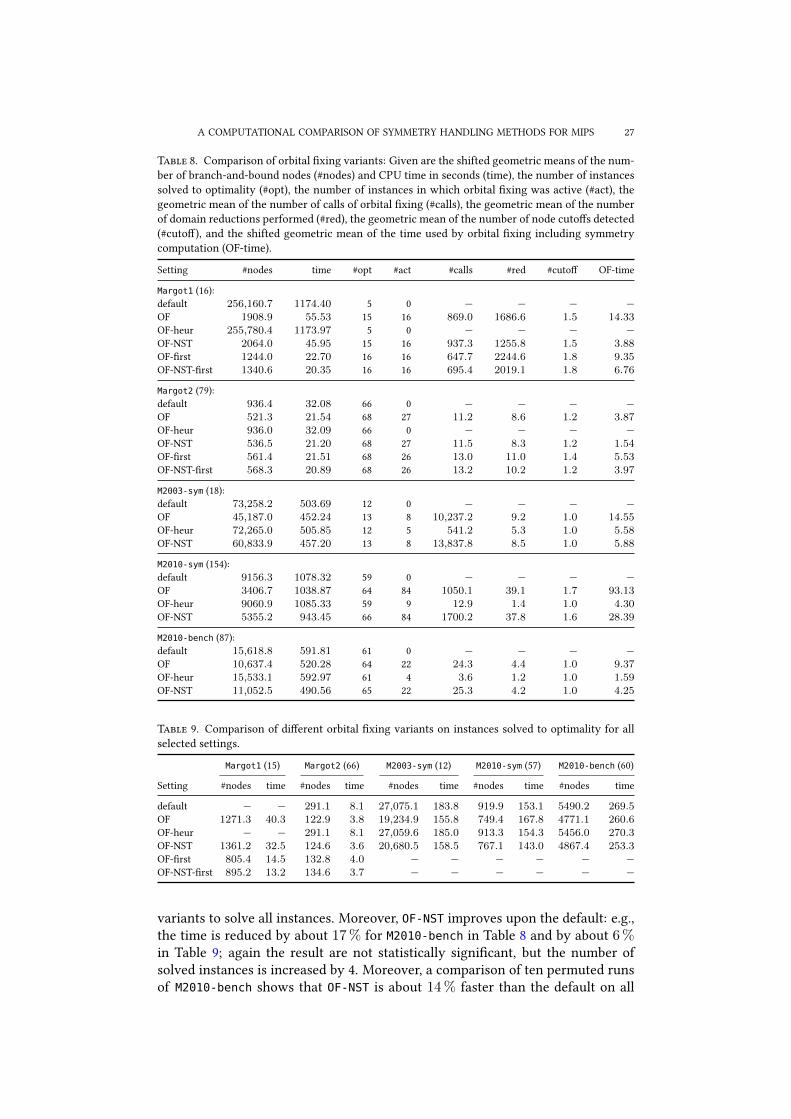
A COMPUTATIONAL COMPARISON OF SYMMETRY HANDLING METHODS FOR MIPS 27
Table 8. Comparison of orbital �xing variants: Given are the shifted geometric means of the num-
ber of branch-and-bound nodes (#nodes) and CPU time in seconds (time), the number of instances
solved to optimality (#opt), the number of instances in which orbital �xing was active (#act), the
geometric mean of the number of calls of orbital �xing (#calls), the geometric mean of the number
of domain reductions performed (#red), the geometric mean of the number of node cuto�s detected
(#cuto�), and the shifted geometric mean of the time used by orbital �xing including symmetry
computation (OF-time).
Setting #nodes time #opt #act #calls #red #cuto� OF-time
Margot1 (16):
default 256,160.7 1174.40 5 0 — — — —
OF 1908.9 55.53 15 16 869.0 1686.6 1.5 14.33
OF-heur 255,780.4 1173.97 5 0 — — — —
OF-NST 2064.0 45.95 15 16 937.3 1255.8 1.5 3.88
OF-�rst 1244.0 22.70 16 16 647.7 2244.6 1.8 9.35
OF-NST-�rst 1340.6 20.35 16 16 695.4 2019.1 1.8 6.76
Margot2 (79):
default 936.4 32.08 66 0 — — — —
OF 521.3 21.54 68 27 11.2 8.6 1.2 3.87OF-heur 936.0 32.09 66 0 — — — —
OF-NST 536.5 21.20 68 27 11.5 8.3 1.2 1.54OF-�rst 561.4 21.51 68 26 13.0 11.0 1.4 5.53
OF-NST-�rst 568.3 20.89 68 26 13.2 10.2 1.2 3.97
M2003-sym (18):
default 73,258.2 503.69 12 0 — — — —
OF 45,187.0 452.24 13 8 10,237.2 9.2 1.0 14.55
OF-heur 72,265.0 505.85 12 5 541.2 5.3 1.0 5.58OF-NST 60,833.9 457.20 13 8 13,837.8 8.5 1.0 5.88
M2010-sym (154):
default 9156.3 1078.32 59 0 — — — —
OF 3406.7 1038.87 64 84 1050.1 39.1 1.7 93.13
OF-heur 9060.9 1085.33 59 9 12.9 1.4 1.0 4.30OF-NST 5355.2 943.45 66 84 1700.2 37.8 1.6 28.39
M2010-bench (87):
default 15,618.8 591.81 61 0 — — — —
OF 10,637.4 520.28 64 22 24.3 4.4 1.0 9.37
OF-heur 15,533.1 592.97 61 4 3.6 1.2 1.0 1.59OF-NST 11,052.5 490.56 65 22 25.3 4.2 1.0 4.25
Table 9. Comparison of di�erent orbital �xing variants on instances solved to optimality for all
selected settings.
Margot1 (15) Margot2 (66) M2003-sym (12) M2010-sym (57) M2010-bench (60)
Setting #nodes time #nodes time #nodes time #nodes time #nodes time
default — — 291.1 8.1 27,075.1 183.8 919.9 153.1 5490.2 269.5OF 1271.3 40.3 122.9 3.8 19,234.9 155.8 749.4 167.8 4771.1 260.6
OF-heur — — 291.1 8.1 27,059.6 185.0 913.3 154.3 5456.0 270.3
OF-NST 1361.2 32.5 124.6 3.6 20,680.5 158.5 767.1 143.0 4867.4 253.3OF-�rst 805.4 14.5 132.8 4.0 — — — — — —
OF-NST-�rst 895.2 13.2 134.6 3.7 — — — — — —
variants to solve all instances. Moreover, OF-NST improves upon the default: e.g.,
the time is reduced by about 17 % for M2010-bench in Table 8 and by about 6 %in Table 9; again the result are not statistically signi�cant, but the number of
solved instances is increased by 4. Moreover, a comparison of ten permuted runs
of M2010-bench shows that OF-NST is about 14 % faster than the default on all

A COMPUTATIONAL COMPARISON OF SYMMETRY HANDLING METHODS FOR MIPS 28
Table 10. Results of orbit probing variants: Given are the shifted geometric means of the number of
branch-and-bound nodes (#nodes) and CPU time in seconds (time), the number of instances solved
to optimality (#opt), the number of instances in which orbit probing was active (#act), the number
of �xed variables (#�xed), and the shifted geometric mean of the time used for probing including
symmetry computation (OP-time).
Setting #nodes time #opt #act #�xed OP-time
Margot1 (16):
default 256,160.7 1174.40 5 0 — 0.00OP 218,782.6 1029.42 6 6 6 0.02
OP-heur 255,654.2 1174.62 5 0 — 0.02
Margot2 (79):
default 936.4 32.08 66 0 — 0.00
OP 714.1 25.45 67 49 96 0.00OP-heur 935.9 32.11 66 0 — 0.00
M2003-sym (18):
default 73,258.2 503.69 12 0 — 0.00OP 67,674.6 485.84 13 5 32 0.20
OP-heur 73,940.5 508.09 12 0 — 0.03
M2010-sym (154):
default 9156.3 1078.32 59 0 — 0.00
OP 7688.5 1095.34 62 44 5272 9.14OP-heur 8926.2 1080.90 59 7 472 1.72
M2010-bench (87):
default 15,618.8 591.81 61 0 — 0.00OP 13,755.9 547.03 64 12 675 2.06
OP-heur 15,495.7 596.39 61 2 90 0.81
Table 11. Comparison of di�erent orbit probing variants on instances solved to optimality for all
selected settings.
Margot1 (5) Margot2 (66) M2003-sym (12) M2010-sym (58) M2010-bench (61)
Setting #nodes time #nodes time #nodes time #nodes time #nodes time
default 30,421.1 92.0 291.1 8.1 27,075.1 183.8 960.1 159.7 5501.3 270.9
OP 21,950.0 71.1 187.2 5.0 25,650.3 176.5 882.1 173.0 5173.0 267.2
OP-heur 30,421.1 92.1 291.1 8.1 27,687.5 186.3 924.0 160.8 5445.8 273.9
instances on average, 5 % faster on the instances solved to optimality for all per-
mutations, and it allows to solve two more instances for all permutations. This
makes orbital �xing a competitive variant.
5.5. Experiment 5: Orbit Probing
We start the evaluation of orbit probing (OP) (see Section 2.5) using the following
two variants:
OP: orbit probing;
OP-heur: OP with heuristic symmetry detection.
The results of these two variants are displayed in Table 10 and 11. The heuristic
symmetry method (OP-heur) again does not improve on the default settings, in
particular, because it is only active for very few instances. Moreover, the results
show that orbit probing �xes relatively few variables, in general. In fact, there is a
small speed-up on Margot1 and Margot2. The results on the MIPLIB instances are
somewhat inconclusive: For M2010-sym and M2010-bench, the number of solved

A COMPUTATIONAL COMPARISON OF SYMMETRY HANDLING METHODS FOR MIPS 29
instances increases by 3. For M2010-sym the time of OP increases with respect
to the default both in Table 10 and 11, while on M2010-bench, the running time
decreases by about 8 % in Table 10, but only very slightly in Table 11.
Consequently, orbit probing should be a candidate for the application together
with other techniques, since it sometimes improves the performance and is rela-
tively inexpensive. We therefore combined orbit probing with isomorphism prun-
ing (OP-ISP-NST), orbital branching (OP-OB-NST), and orbital �xing (OP-OF-NST).
However, the results show that these variants often solve less instances and are
generally slower. We therefore only present the corresponding tables in the on-
line supplement. The somewhat surprising outcome is that orbit probing does not
seem to improve the performance of other methods.
5.6. Experiment 6: Symmetry Breaking Ineqalities
With respect to symmetry breaking constraints, we investigate the following vari-
ants as described in Section 2.6:
S: add inequalities (3), (4), (5) or orbitopes if applicable;
S-fund: variant S with fundamental domain inequalities (6);
S-fundnolp: variant S with (6) handled in propagation, but not added to the LP;
S-nolp: as variant S, but do not add inequalities to LP – instead propagate them;
S-prob: variant S with probing;
S-orbitmin: add inequalities (3) for all orbits using the minimal element;
S-heur: as variant S, but use heuristic detection of symmetry.
Table 12 reports the results on symmetry breaking inequalities and Table 13
shows a comparison on the instances solved to optimality.
As for the other methods, the heuristic variant S-heur is not able to improve
on variant S. In this case, this is even more surprising, since the added inequalities
essentially only exploit symmetric groups. Obviously, this variant is missing the
matrix operations in order to perform better. Note, however, that S-heur adds
more inequalities for M2010-sym and M2010-bench than all other variants. This
is mainly due to a few instances for which the largest share of inequalities is
generated. In the other methods, the limit on the number of generators avoids
similarly large groups and numbers.
For the Margot instances, only S-orbitmin and S-fund are able to improve on
the default settings. But the running times are still an order of magnitude slower
that isomorphism pruning. All other variants are not able to perform better, be-
cause no structures like full symmetric subgroups could be found.
For the MIPLIB instances, S-orbitmin seems to be the best variant and per-
forms well: it increases the number of solved instances by four for M2010-sym and
by two for M2010-bench. Moreover, the running time is improved by about 18 %for M2003-sym, 12 % for M2010-sym, and 13 % for M2010-bench with respect to the
number of instances solved to optimality by variants, see Table 13. These results
are statistically signi�cant for M2010-bench with a p-value of less than 0.05. All
other variants (except S-heur and S-fund on M2010-sym) are also able to improve
on the default. Note that three orbitope structures are found for M2010-sym and
one for M2010-bench. Moreover, probing slightly improves on variant S for on
these three testsets, but is not faster than S-orbitmin.

A COMPUTATIONAL COMPARISON OF SYMMETRY HANDLING METHODS FOR MIPS 30
Table 12. Comparison of di�erent symmetry breaking inequality variants: Given are the shifted
geometric means of the number of branch-and-bound nodes (#nodes) and CPU time in seconds
(time), the number of instances solved to optimality (#opt), the number of instances in which in-
equalities were added (#act), the number of handled full symmetric groups (#full), the number of
fundamental domains handled (#fund), the number of orbitope structures found (#orb), the number
of cyclic groups handled, the total number of inequalities added (#tot), and the shifted geometric
mean of the time used for adding inequalities including symmetry computation (sym-time).
Setting #nodes time #opt #act #full #fund #orb #cyc #tot #�xed sym-time
Margot1 (16):
default 256,160.7 1174.40 5 0 — — — — — — 0.00
S 256,404.3 1174.58 5 0 — — — — — — 0.10
S-fund 169,229.1 972.17 6 16 — 145 — — 145 — 0.11S-fundnolp 254,833.0 1181.44 5 16 — 145 — — 145 — 0.11
S-nolp 256,483.4 1174.78 5 0 — — — — — — 0.11
S-prob 256,435.9 1176.01 5 0 — — — — — — 0.10S-orbitmin 104,817.7 523.54 9 16 — — — 16 3794 — 0.13
S-heur 256,060.4 1174.32 5 0 — — — — — — 0.02
Margot2 (79):
default 936.4 32.08 66 0 — — — — — — 0.00
S 936.2 32.17 66 0 — — — — — — 0.05S-fund 888.1 30.71 67 70 — 524 — — 524 — 0.05
S-fundnolp 976.1 33.29 65 70 — 524 — — 524 — 0.05
S-nolp 936.3 32.16 66 0 — — — — — — 0.04S-prob 936.3 32.16 66 0 — — — — — — 0.05
S-orbitmin 596.0 23.77 68 70 — — — 70 10,118 — 0.06
S-heur 936.3 32.10 66 0 — — — — — — 0.00
M2003-sym (18):
default 73,258.2 503.69 12 0 — — — — — — 0.00S 69,721.1 459.57 12 16 114 — — — 168 — 0.14
S-fund 65,028.8 440.50 12 18 114 91 — — 259 — 0.14
S-fundnolp 70,759.7 496.32 12 18 114 91 — — 259 — 0.14S-nolp 71,738.6 496.71 12 16 114 — — — 168 — 0.14
S-prob 60,392.0 438.47 12 16 114 — — — 168 65 0.14
S-orbitmin 65,606.0 443.83 12 18 — — — 121 185 — 0.03S-heur 72,697.2 492.18 12 10 54 — — — 83 — 0.02
M2010-sym (154):
default 9156.3 1078.32 59 0 — — — — — — 0.00
S 8915.2 1054.44 60 114 9838 — 3 — 19,745 6058 3.31
S-fund 8299.3 1076.28 60 152 9838 2154 3 — 21,899 6058 3.32S-fundnolp 8367.2 1027.87 61 152 9838 2154 3 — 21,899 6058 3.33
S-nolp 8601.0 1050.37 60 114 9838 — 3 — 19,745 6058 3.31
S-prob 8756.3 1061.90 59 114 9838 — 3 — 19,745 6367 3.42S-orbitmin 8216.3 1005.91 63 153 — — — 9949 23,961 — 1.40
S-heur 9058.9 1107.73 57 49 40,629 — — — 140,111 — 1.62
M2010-bench (87):
default 15,618.8 591.81 61 0 — — — — — — 0.00
S 15,588.7 579.48 61 31 1439 — 1 — 5614 3 0.61S-fund 15,475.1 584.52 61 39 1439 90 1 — 5704 3 0.61
S-fundnolp 14,553.5 552.50 63 39 1439 90 1 — 5704 3 0.61
S-nolp 14,915.8 569.11 62 31 1439 — 1 — 5614 3 0.61S-prob 15,052.8 575.28 61 31 1439 — 1 — 5614 33 0.64S-orbitmin 13,558.2 531.99 63 39 — — — 1457 5723 — 0.55
S-heur 15,675.1 605.22 60 14 9214 — — — 52,729 — 0.73

A COMPUTATIONAL COMPARISON OF SYMMETRY HANDLING METHODS FOR MIPS 31
Table 13. Comparison of di�erent symmetry breaking inequality variants on instances solved to
optimality for all selected settings.
Margot1 (5) Margot2 (65) M2003-sym (12) M2010-sym (55) M2010-bench (60)
Setting #nodes time #nodes time #nodes time #nodes time #nodes time
default 30,421.1 92.0 241.7 6.8 27,075.1 183.8 912.6 153.2 5317.8 262.2
S 30,421.1 92.1 241.7 6.8 25,824.1 159.3 904.8 144.7 5303.3 252.2S-fund 16,435.0 71.6 228.8 6.5 23,259.2 149.1 896.9 154.5 5267.8 255.5
S-fundnolp 29,690.4 94.0 252.9 7.2 26,730.4 179.7 814.1 139.9 4964.2 239.6S-nolp 30,421.1 92.2 241.7 6.8 26,863.4 179.8 857.1 143.7 5098.9 248.1
S-prob 30,421.1 92.5 241.7 6.8 20,411.1 148.0 830.8 143.0 5053.7 249.7
S-orbitmin 4025.4 15.3 114.6 3.4 24,015.4 150.9 774.1 134.7 4552.7 227.3S-heur 30,421.1 92.0 241.7 6.8 27,017.4 177.3 895.9 154.1 5349.9 267.9
In total, we conclude that adding Inequalities (3) for each orbit (S-orbitmin)
performs better than adding Inequalities (4) for each full symmetric group fac-
tor (variant S). Moreover, we checked the behavior of the root-LP bound, which
very slightly improves for S-orbitmin, but not for variant S. We have to leave it
to future research to understand these outcomes and possibly improve on these
results.
5.7. Experiment 7: Projection on the Fixed Space
The projection on the �xed space is only useful for instances that contain contin-
uous variables. Thus, we do not report results on the Margot testsets. Moreover,
we also study the following combination with other variants:
lpfix: default �xing as described in Section 2.7;
lpfix-heur: lpfix with heuristic symmetry group computation;
lpfix-OP: lpfix together with orbit probing variant OP;
lpfix-fundnolp: lpfix together with variant S-fundnolp;
lpfix-orbitmin: lpfix together with variant S-orbitmin.
The results are shown in Table 14 and 15. Both lpfix and lpfix-heur were
able to �x quite a number of variables. For M2003-sym nothing can be gained.
For M2010-sym and M2010-bench all variants except lpfix-heur slightly improve
on the default, but the improvements are only minor. In total, the LPs become
smaller, but the bene�t is obviously not large. Moreover, the performance of the
combination lpfix-orbitmin is worse that running S-orbitmin alone. One rea-
son is that for lpfix CVR symmetries are needed. This in general decreases the
size of the symmetry group and therefore the number of generated inequalities.
However, as a stand-alone this �xing can essentially be performed without caus-
ing harm and might be able to improve the performance on instances with very
large symmetries on continuous variables.
5.8. Experiment 8: Comparison of the Different Methods
In order to get an overall picture, we compare the best symmetry handling vari-
ants in Tables 16 and 17. We obtain the following results:
Margot1. ISP-NST-first is the winner, closely followed by OF-NST-first. These
two are the only variants that solve all instances. They are followed by OB-NST,
OB, ISP-NST, OF-NST, ISP, and OF. However, all these variants are extremely fast in
comparison to the default settings. In essence, these results prove the theoretical

A COMPUTATIONAL COMPARISON OF SYMMETRY HANDLING METHODS FOR MIPS 32
Table 14. Results of LP �xing variants: Given are the shifted geometric means of the number of
branch-and-bound nodes (#nodes) and CPU time in seconds (time), the number of instances solved
to optimality (#opt), the number of instances in which LP �xing was active (#act), the number of
�xed variables, and the shifted geometric mean of the time used for �xing including symmetry
computation (lp�x-time).
Setting #nodes time #opt #act #�xed lp�x-time
M2003-sym (18):
default 73258.2 503.69 12 0 — 0.00lp�x 74935.4 526.29 12 4 88 0.04
lp�x-heur 73355.6 500.27 12 3 7 0.02
lp�x-OP 72417.7 502.68 12 3 12 0.01lp�x-fundnolp 74982.6 526.05 12 4 88 0.04
lp�x-orbitmin 81421.2 583.75 13 4 88 0.05
M2010-sym (154):
default 9156.3 1078.32 59 0 — 0.00
lp�x 9128.0 1065.30 59 23 10,676 0.28lp�x-heur 9292.8 1084.79 58 17 12,383 0.23
lp�x-OP 9149.1 1067.00 59 22 10,619 0.06
lp�x-fundnolp 9156.2 1065.33 59 23 10,676 0.58lp�x-orbitmin 9339.9 1075.01 60 23 10,676 0.56
M2010-bench (87):
default 15618.8 591.81 61 0 — 0.00
lp�x 15095.2 581.61 61 8 836 0.11
lp�x-heur 15831.1 601.28 60 5 156 0.08lp�x-OP 15199.9 583.77 61 7 779 0.03
lp�x-fundnolp 15182.2 582.53 61 8 836 0.29
lp�x-orbitmin 15186.4 583.72 61 8 836 0.29
Table 15. Comparison of di�erent LP �xing variants on instances solved to optimality for all se-
lected settings.
M2003-sym (12) M2010-sym (58) M2010-bench (60)
Setting #nodes time #nodes time #nodes time
default 27,075.1 183.8 933.1 154.3 5317.8 262.2
lp�x 28,138.4 196.7 895.5 149.6 5131.3 256.4lp�x-heur 27,238.3 181.9 945.1 154.9 5383.3 265.3
lp�x-OP 26,729.3 183.3 902.2 150.1 5165.1 257.5
lp�x-fundnolp 28,138.4 196.6 903.3 149.6 5177.0 257.0lp�x-orbitmin 28,138.4 197.0 903.3 149.7 5177.0 257.8
arguments of [38] that orbital branching performs similar to isomorphism prun-
ing. However, the branching rule for isomorphism pruning plays a signi�cant role
for these instances and allows to change the ranking.
Margot2. Here, the performance of all variants based on isomorphism pruning
or orbital branching is quite close together and no variant dominates the others.
Variant ISP-NST-first solves the largest number of instances.
M2003-sym. Again the performance of the variants based on ISP or OB is quite
close together and no variant dominates the others. Variants ISP, ISP-NST, OF, and
OF-NST solve the largest number of instances (one more than the default settings).
In terms of time OB-NST and S-orbitmin are best (with respect to Tables 16 and 17,
respectively), but both solve one instances less.
M2010-sym. Here, ISP-NST solves 67 instances, followed by OF-NST with 66 in-
stances. All other variants (except the orbital branching variants) still solve more

A COMPUTATIONAL COMPARISON OF SYMMETRY HANDLING METHODS FOR MIPS 33
Table 16. Comparison of di�erent symmetry handling variants.
Setting #nodes time #opt #act method-time sym-time
Margot1 (16):
default 256,160.7 1174.40 5 0 0.45 0.00
ISP 1787.0 54.40 15 16 17.27 0.02ISP-NST 2041.0 45.01 15 16 4.25 0.02
ISP-NST-�rst 934.0 14.86 16 16 5.41 0.02
OB 1916.9 39.91 15 16 10.72 0.02OB-NST 2119.0 37.01 15 16 0.95 0.02
OF 1908.9 55.53 15 16 14.30 0.02
OF-NST 2064.0 45.95 15 16 3.87 0.02OF-NST-�rst 1340.6 20.35 16 16 6.74 0.02
S 256,404.3 1174.58 5 16 0.57 0.00
S-orbitmin 104,817.7 523.54 9 16 0.46 0.00
Margot2 (79):
default 936.4 32.08 66 0 0.08 0.00ISP 519.9 21.72 68 59 4.91 0.00
ISP-NST 541.2 21.30 67 59 1.73 0.00
ISP-NST-�rst 574.4 20.89 69 59 4.64 0.00OB 527.6 20.65 68 59 3.69 0.00
OB-NST 536.3 20.37 68 59 0.17 0.00
OF 521.3 21.54 68 59 3.88 0.00OF-NST 536.5 21.20 68 59 1.56 0.00
OF-NST-�rst 568.3 20.89 68 59 4.00 0.00S 936.2 32.17 66 77 0.13 0.00
S-orbitmin 596.0 23.77 68 77 0.13 0.00
M2003-sym (18):
default 73,258.2 503.69 12 0 0.67 0.00
ISP 44,314.2 453.66 13 16 16.41 0.03
ISP-NST 60,763.2 458.55 13 16 6.93 0.03OB 32,653.7 472.14 11 16 61.53 0.03
OB-NST 38,787.1 438.62 12 16 5.57 0.03OF 45,187.0 452.24 13 16 14.72 0.03
OF-NST 60,833.9 457.20 13 16 6.02 0.03
S 69,721.1 459.57 12 18 0.76 0.00S-orbitmin 65,606.0 443.83 12 18 0.69 0.00
M2010-sym (154):
default 9156.3 1078.32 59 0 0.38 0.00ISP 3218.8 1070.14 63 144 88.46 1.23
ISP-NST 5074.6 942.52 67 144 27.23 1.24OB 3637.5 1305.89 54 142 243.24 1.26
OB-NST 5334.5 1193.96 57 142 45.24 1.26
OF 3406.7 1038.87 64 144 86.47 1.25OF-NST 5355.2 943.45 66 144 25.20 1.25
S 8915.2 1054.44 60 153 3.75 0.00
S-orbitmin 8216.3 1005.91 63 153 1.81 0.00
M2010-bench (87):
default 15,618.8 591.81 61 0 0.38 0.00ISP 10,673.1 519.32 65 36 9.31 0.52
ISP-NST 10,867.6 487.90 65 36 4.23 0.52OB 11,684.8 691.72 56 36 26.45 0.52OB-NST 12,897.0 647.10 59 36 9.34 0.52
OF 10,637.4 520.28 64 36 8.97 0.52
OF-NST 11,052.5 490.56 65 36 3.95 0.52S 15,588.7 579.48 61 40 1.01 0.00
S-orbitmin 13,558.2 531.99 63 40 0.94 0.00
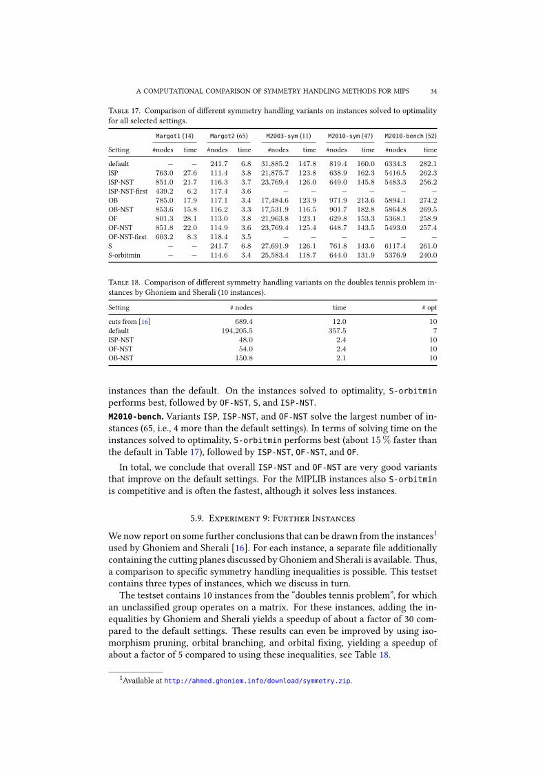
A COMPUTATIONAL COMPARISON OF SYMMETRY HANDLING METHODS FOR MIPS 34
Table 17. Comparison of di�erent symmetry handling variants on instances solved to optimality
for all selected settings.
Margot1 (14) Margot2 (65) M2003-sym (11) M2010-sym (47) M2010-bench (52)
Setting #nodes time #nodes time #nodes time #nodes time #nodes time
default — — 241.7 6.8 31,885.2 147.8 819.4 160.0 6334.3 282.1
ISP 763.0 27.6 111.4 3.8 21,875.7 123.8 638.9 162.3 5416.5 262.3ISP-NST 851.0 21.7 116.3 3.7 23,769.4 126.0 649.0 145.8 5483.3 256.2
ISP-NST-�rst 439.2 6.2 117.4 3.6 — — — — — —
OB 785.0 17.9 117.1 3.4 17,484.6 123.9 971.9 213.6 5894.1 274.2
OB-NST 853.6 15.8 116.2 3.3 17,531.9 116.5 901.7 182.8 5864.8 269.5
OF 801.3 28.1 113.0 3.8 21,963.8 123.1 629.8 153.3 5368.1 258.9OF-NST 851.8 22.0 114.9 3.6 23,769.4 125.4 648.7 143.5 5493.0 257.4
OF-NST-�rst 603.2 8.3 118.4 3.5 — — — — — —
S — — 241.7 6.8 27,691.9 126.1 761.8 143.6 6117.4 261.0S-orbitmin — — 114.6 3.4 25,583.4 118.7 644.0 131.9 5376.9 240.0
Table 18. Comparison of di�erent symmetry handling variants on the doubles tennis problem in-
stances by Ghoniem and Sherali (10 instances).
Setting # nodes time # opt
cuts from [16] 689.4 12.0 10default 194,205.5 357.5 7
ISP-NST 48.0 2.4 10
OF-NST 54.0 2.4 10OB-NST 150.8 2.1 10
instances than the default. On the instances solved to optimality, S-orbitmin
performs best, followed by OF-NST, S, and ISP-NST.
M2010-bench. Variants ISP, ISP-NST, and OF-NST solve the largest number of in-
stances (65, i.e., 4 more than the default settings). In terms of solving time on the
instances solved to optimality, S-orbitmin performs best (about 15 % faster than
the default in Table 17), followed by ISP-NST, OF-NST, and OF.
In total, we conclude that overall ISP-NST and OF-NST are very good variants
that improve on the default settings. For the MIPLIB instances also S-orbitmin
is competitive and is often the fastest, although it solves less instances.
5.9. Experiment 9: Further Instances
We now report on some further conclusions that can be drawn from the instances1
used by Ghoniem and Sherali [16]. For each instance, a separate �le additionally
containing the cutting planes discussed by Ghoniem and Sherali is available. Thus,
a comparison to speci�c symmetry handling inequalities is possible. This testset
contains three types of instances, which we discuss in turn.
The testset contains 10 instances from the “doubles tennis problem”, for which
an unclassi�ed group operates on a matrix. For these instances, adding the in-
equalities by Ghoniem and Sherali yields a speedup of about a factor of 30 com-
pared to the default settings. These results can even be improved by using iso-
morphism pruning, orbital branching, and orbital �xing, yielding a speedup of
about a factor of 5 compared to using these inequalities, see Table 18.
1Available at http://ahmed.ghoniem.info/download/symmetry.zip.

A COMPUTATIONAL COMPARISON OF SYMMETRY HANDLING METHODS FOR MIPS 35
The 40 instances from the “noise dosage problem” have symmetric groups op-
erating on a matrix, but do not contain binary variables. Thus, using our imple-
mentations of isomorphism pruning, orbital branching, and orbital �xing do not
apply any reductions. Adding symmetry breaking inequalities slightly improves
on the default settings, but is clearly dominated by using the inequalities in [16].
Finally, the 120 instances for “wagon load-balancing problem” have unclassi-
�ed symmetry groups and contain mainly binary variables. The particular struc-
ture of these instances make all our symmetry handling methods extremely slow.
Both computing stabilizers and lexicographic representatives requires a very large
computation time and memory. Thus, the inequalities in [16] are clearly superior.
Moreover, even if the local symmetry group is computed (which can be done ef-
�ciently), our methods fail to improve on the case where the inequalities of [16]
are used. Obviously, these inequalities help to improve the lower bounds using
further cutting planes, while the other techniques do not allow to do this.
We have to leave the development of general symmetry handling methods for
such instances to future research.
6. Conclusion
The nine experiments above allow to reach the following conclusions:
◦ Isomorphism pruning and orbital �xing allow for a speed-up of two orders of
magnitude for solving special instances like the instances of Margot, but also
allow a decent speed-up on instances like the ones in the MIPLIB.
◦ Orbital branching also performs very well on the particular instances of Mar-
got, but does not perform too well on the MIPLIB instances, mainly because
the branching rule needs to be coordinated with the other rules.
◦ The instances of Margot, used both to test isomorphism pruning and orbital
�xing in the literature, have a quite special structure. In particular, �rst index
branching signi�cantly helps isomorphism pruning on these instances, while
it does not help the default.
◦ While there are many coordinate actions of symmetric groups, the heuristic
symmetry detection used in any of the methods does not bene�t from this and
almost never allows for a speed-up.
◦ Adding Inequalities (3) for each orbit seems to be a quite good idea for general
MIPLIB instances. All other inequalities perform less well.
◦ The �xing of continuous variables slightly speeds up LP-solving, but does not
result in a signi�cant overall speed-up. It can nevertheless be applied, since
it also does not create overhead and might help for very symmetric instances
involving continuous variables.
◦ The performance of orbit probing is somewhat disappointing.
◦ Symmetry detection is not a bottleneck, while the computation of stabilizers
and lexicographical tests can be.
This suggests the following future research:
◦ The performance of the symmetry handling methods should be improved by
tuning parameters that automatically avoid symmetry handling if this is likely
to not help or would take a long time. Moreover, methods to avoid very large
computation times like on the instances of Ghoniem and Sherali should be
developed if possible.

A COMPUTATIONAL COMPARISON OF SYMMETRY HANDLING METHODS FOR MIPS 36
◦ The special structure of matrix actions of symmetric groups should be ex-
ploited to speed-up both the detection of symmetries and the computation of
stabilizers and the like.
◦ Possibly orbit probing can be turned into an interesting method.
◦ It seems that particular inequalities can help to improve the dual bound – see
the instances of Ghoniem and Sherali. More research is needed to �nd general
purpose inequalities with the same behavior.
In conclusion, it seems that there are several ways in which the handling of sym-
metries might improve in the future, even though many techniques are already
available and used in practice.
Appendix A. List of MIPLIB 2010 symmetries
The following table lists details about the symmetry groups of MIPLIB 2010 in-
stances. The second column shows the logarithm to the base 10 of the order of
the symmetry groups. The third column presents the percentage of variables that
lie in an orbit of at least size two, i.e., variables on which the symmetry group acts
non-trivially. The fourth column shows the groups which the symmetry group is
a direct product of. The following notation is used:
◦ Sk denotes a symmetric group of degree k in coordinate action;
◦ M(G, `) represents the matrix action of group G on ` points.
◦ “unknown” denotes groups whose type could not be determined by PermLib.
The computations for this table were performed on an Intel i7 CPU with 3.40
GHz and 32 GB of memory and a time limit of 10 hours. For some instances, the
computation or analysis ran into the memory or time limit. These instances are
marked with "—". Instances without symmetry are not shown.
Table 19. List of (possibly) symmetric MIPLIB 2010 instances before presolving. Additionally the
log10 of the order of their symmetry groups and the number of variables involved in a nontrivial
symmetry is shown.
name log10 |G| #vars factors
30_70_45_095_100 0.4 0.0 S2acc-tight4 4.7 97.8 1 unknown
ash608gpia-3col 0.8 100.0 M(S3, 3651)atlanta-ip 4450.0 40.5 (S2)5898, (S3)1441, (S4)284, (S5)175, (S6)165, (S7)88bab3 70.1 9.5 (S2)10, (S5)16, (S6)4, (S10)2, (M(S2, 12328))3,
4 unknown
bab5 1.3 17.9 (M(S2, 968))4beasleyC3 0.7 0.6 (M(S2, 8))2biella1 217.3 11.7 (S2)261, (S3)30, (S4)20, (S5)13, (S6)2, (S7)5, S8, (S9)2,
(S10)2, S11blp-ar98 0.7 0.0 (S2)2blp-ic97 0.7 0.0 (S2)2bnatt350 503.7 43.3 (S2)42, (S3)81, (S4)88, (S5)76, (S6)39, (S7)10bnatt400 588.0 43.6 (S2)50, (S3)83, (S4)98, (S5)91, (S6)42, (S7)16, S8circ10-3 1.4 100.0 1 unknown
co-100 736.0 6.3 (S2)837, (S3)399, (S4)3, (S5)3, S6, (S7)2, S12, S17, S19,
S21, S28, S29, S30
continued on next page . . .

A COMPUTATIONAL COMPARISON OF SYMMETRY HANDLING METHODS FOR MIPS 37
name log10 |G| #vars factors
core2536-691 3.7 0.1 (S2)5, S5core4872-1529 68.9 2.0 (S2)211, (S3)2, S6, M(S2, 8), M(S2, 14), M(S2, 28)cov1075 6.6 100.0 1 unknown
datt256 3.7 0.0 (S2)12dc1c 356.6 19.8 (S2)819, (S3)64, (S4)24, (S5)2, (S6)8dc1l 794.9 11.4 (S2)1640, (S3)174, (S4)69, (S5)18, (S6)9, (S7)2dg012142 89.2 3.1 S64dolom1 468.2 19.4 (S2)907, (S3)71, (S4)25, (S5)5, (S7)2, S15, S33, S34ds-big 468.1 1.8 (S2)1516, (S3)15eilB101 0.8 0.1 S3enlight13 0.4 92.3 M(S2, 312)enlight14 0.4 92.9 M(S2, 364)enlight15 0.4 93.3 M(S2, 420)enlight16 0.4 93.8 M(S2, 480)enlight9 0.4 88.9 M(S2, 144)ex1010-pi 1482.1 21.7 (S2)1324, (S3)366, (S4)148, (S5)70, (S6)32, (S7)27,
(S8)20, (S9)13, (S10)3, (S11)5, S12, (S16)2ex10 1.0 100.0 1 unknown
ex9 30.2 100.0 1 unknown
glass4 0.4 0.6 S2gmu-35-40 801.6 39.3 (S2)18, (S3)16, (S4)3, (S5)3, S363gmu-35-50 1837.7 44.5 (S2)18, (S3)16, (S4)3, (S5)3, S742gmut-75-50 — — —
gmut-77-40 40,582.7 47.2 (S2)12, (S3)7, (S4)20, (S5)31, S11198go19 3.5 99.8 S4, 1 unknown
iis-bupa-cov 2.2 2.0 S3, S4iis-pima-cov 35.5 4.2 S32lectsched-1 624.4 12.4 (S2)3, (S3)3, S193, (M(S2, 4))797, (M(S3, 6))18,
(M(S4, 8))6lectsched-1-obj 624.4 12.4 (S2)3, (S3)3, S193, (M(S2, 4))797, (M(S3, 6))18,
(M(S4, 8))6lectsched-2 408.6 11.7 (S2)3, S148, (M(S2, 4))462, (M(S3, 6))6, (M(S4, 8))4lectsched-3 543.9 10.9 (S2)3, (S3)3, S184, (M(S2, 4))633, (M(S3, 6))15lectsched-4-obj 217.1 13.2 S93, (M(S2, 4))230, (M(S3, 6))3, M(S4, 8)liu 0.4 0.2 S2macrophage 61.2 25.0 (S2)146, (M(S2, 4))15, (M(S2, 6))9, (M(S2, 12))2,
M(S2, 14), M(S4, 24), M(S6, 48), M(S2 × S2, 14),2 unknown
map06 — — —
map10 — — —
map14 — — —
map18 — — —
map20 — — —
maxgas�ow 5.5 1.8 (M(S2, 6))11, M(S2, 12), M(S2, 24), M(S3, 12),M(S3, 18)
mcsched 4.6 5.2 (M(S2, 6))15methanosarcina 762.7 64.7 (S2)2505, M(S2 o S2, 28), 4 unknown
mkc 77.2 61.3 (S2)9, (S3)4, (M(S2, 4))15, (M(S2, 6))3, (M(S2, 8))2,
M(S2, 10), (M(S2, 12))2, M(S2, 24), M(S2, 28),(M(S3, 6))6, M(S3, 9), (M(S3, 12))2, M(S3, 18),(M(S3, 24))2, M(S3, 42), (M(S4, 8))4, M(S4, 48),(M(S5, 10))2, M(S6, 60), M(S7, 14), M(S8, 16),5 unknown
continued on next page . . .

A COMPUTATIONAL COMPARISON OF SYMMETRY HANDLING METHODS FOR MIPS 38
name log10 |G| #vars factors
momentum3 36.7 0.9 (M(S3, 6))2, M(S5, 10), M(S6, 12), M(S7, 14),(M(S9, 18))3, M(S13, 26)
msc98-ip 2673.2 33.2 (S2)609, (S3)266, (S4)219, (S5)198, (S6)210, (S7)108,
(S8)112, (S9)2, (S10)6, (M(S2, 14))2, M(S2, 24),M(S2, 26), M(S2, 34), M(S2, 38), S2 o S2
mzzv11 46.7 3.0 (S2)155n3seq24 9.9 11.4 M(S2, 48), (M(S2, 50))4, (M(S2, 54))2, (M(S2, 62))4,
M(S2, 72), (M(S2, 90))4, (M(S2, 110))2, M(S2, 142),(M(S2, 180))2, M(S2, 296), (M(S2, 490))2,
M(S2, 798), M(S2, 1018), M(S2, 3878), M(S2, 4772),M(S4, 180)
nag 0.4 0.1 S2neos-1109824 1.7 100.0 1 unknown
neos-1171692 19.8 100.0 M(S21, 1638)neos-1171737 32.5 100.0 M(S30, 2340)neos-1224597 504.2 100.0 (S5)17, (S10)3, S35, 2 unknown
neos-1311124 78.9 100.0 M(S21, 84), (M(S21, 168))2, M(S21, 672)neos-1337307 3.8 87.5 M(S7, 2485)neos-1396125 0.8 78.3 M(S3, 909)neos13 0.4 0.1 S2neos-1426635 26.3 100.0 M(S10, 40), (M(S10, 80))2, M(S10, 320)neos-1426662 53.4 100.0 M(S16, 64), (M(S16, 128))2, M(S16, 512)neos-1429212 — — —
neos-1436709 39.2 100.0 M(S13, 52), (M(S13, 104))2, M(S13, 416)neos-1440460 22.3 100.0 M(S9, 36), (M(S9, 72))2, M(S9, 288)neos-1442119 43.8 100.0 M(S14, 56), (M(S14, 112))2, M(S14, 448)neos-1442657 34.8 100.0 M(S12, 48), (M(S12, 96))2, M(S12, 384)neos-1601936 432.5 9.2 S72, 1 unknown
neos-1605061 103.8 1.8 S72neos-1605075 103.8 1.7 S72neos-1620770 3.8 97.2 1 unknown
neos18 247.9 36.1 (S2)6, (S3)2, (S4)2, (M(S2, 4))28, (M(S2, 8))3,
(M(S3, 6))2, (M(S3, 12))3, (M(S4, 8))19,
(M(S4, 16))3, M(S6, 12), M(S8, 16), (S2 o S2)2,
(S2 o S9)4, (S2 o S11)2, M(S2 o S10, 40), M(S2 o S6, 24),
M(S2 o S7, 28), M(S2 o S6, 24), M(S2 o S9, 36),M(S2 o S9, 36), M(S2 o S11, 44), M(S2 o S8, 32),M(S2 o S7, 28), M(S2 o S10, 40), M(S2 o S3, 12),
M(S2 o S10, 40), M(S2 o S13, 52), M(S2 o S2, 8),M(S2 o S2, 8), M(S2 o S5, 20), M(S2 o S3, 12),
M(S2 o S3, 12), M(S2 o S10, 40), M(S2 o S4, 16),
M(S2 o S3, 12), M(S2 o S9, 36), M(S2 o S2, 8),M(S2 o S2, 8), M(S2 o S2, 8), M(S2 o S2, 8)
neos-476283 39.9 1.1 S7, S27, (M(S2, 4))10, (M(S2, 24))2, S5 o S2
neos-555424 146.4 99.9 M(S10, 20), (M(S10, 300))2, M(S20, 40), M(S30, 60),M(S10 o S3, 90), M(S10 o S3, 90), 1 unknown
neos-631710 313.7 99.7 M(S11, 6094), M(S15, 8325), M(S15, 8340),M(S16, 8864), M(S18, 9990), M(S19, 10564),M(S24, 13344), M(S28, 15540), M(S33, 18282),M(S39, 21645), M(S40, 22160), M(S42, 23352)
neos6 6.6 94.9 M(S10, 8340)neos-738098 21.0 93.5 1 unknown
neos-777800 1.0 100.0 1 unknown
neos-785912 9.8 91.3 1 unknown
neos788725 0.7 100.0 1 unknown
neos808444 0.4 11.5 M(S2, 2288)neos-820146 106.2 100.0 1 unknown
neos-820157 557.8 100.0 1 unknown
continued on next page . . .

A COMPUTATIONAL COMPARISON OF SYMMETRY HANDLING METHODS FOR MIPS 39
name log10 |G| #vars factors
neos-824661 936.3 100.0 1 unknown
neos-824695 936.3 100.0 1 unknown
neos-826650 475.2 98.6 2 unknown
neos-826694 973.0 99.3 2 unknown
neos-826812 141.1 99.3 1 unknown
neos-826841 41.5 98.5 1 unknown
neos-849702 3.7 100.0 1 unknown
neos-859770 769.1 98.9 (S2)11, S6, S12, S20, S25, S32, 1 unknown
neos-885086 56.1 100.0 M(S45, 4860)neos-885524 — — —
neos-911880 7.6 100.0 (M(S3, 111))6, M(S6, 222)neos-932816 598.6 85.3 S293, M(S4, 17628)neos-933638 1184.6 93.9 S42, S495, 3 unknown
neos-933966 1183.6 95.7 S42, S495, M(S2, 1218), M(S3, 1827), 3 unknown
neos-934278 1709.5 81.4 S389, S396, M(S2, 1056), 5 unknown
neos-935627 5817.1 75.9 S2022, M(S2, 236), 5 unknown
neos-935769 5817.5 80.9 S2022, M(S3, 354), M(S3, 360), M(S3, 387),M(S3, 405), 5 unknown
neos-937511 5261.9 79.7 S1853, M(S3, 408), M(S3, 423), M(S3, 465),M(S3, 480), 5 unknown
neos-937815 5335.7 72.6 S1876, M(S2, 264), M(S2, 266), M(S2, 276), 5 unknown
neos-941262 5570.5 76.3 S1948, M(S2, 170), M(S2, 204), M(S2, 220),M(S2, 248), (M(S2, 282))2, M(S2, 292), M(S2, 298),M(S2, 310), 4 unknown
neos-941313 — — —
neos-948126 4969.9 78.9 S1764, M(S2, 204), M(S2, 222), M(S2, 234),M(S2, 238), M(S2, 282), M(S2, 298), 5 unknown
neos-952987 16.5 0.3 (S2)36, S9neos-957389 33.8 75.1 M(S2, 126), (M(S4, 280))2, M(S10, 690), M(S10, 700),
1 unknown
neos-984165 4280.8 75.8 (S2)11, S1549, M(S2, 152), M(S2, 206), M(S2, 218),M(S2, 222), M(S2, 240), M(S2, 260), M(S2, 266),M(S2, 286), 4 unknown
noswot 0.4 40.6 M(S2, 52)ns1111636 — — —
ns1116954 553.4 99.9 2 unknown
ns1158817 — — —
ns1208400 2.8 97.8 1 unknown
ns1456591 36.8 99.8 S20, M(S20, 8360)ns1606230 103.8 1.7 S72ns1631475 31.7 0.9 (S2)105ns1702808 2.9 100.0 M(S6, 804)ns1758913 0.4 3.0 M(S2, 540)ns1830653 15.9 1.1 S18ns1853823 0.7 56.1 1 unknown
ns1854840 2.0 88.0 1 unknown
ns1856153 0.4 92.5 M(S2, 11102)ns1905797 1.4 100.0 M(S4, 18192)ns1905800 1.1 100.0 1 unknown
ns1952667 69.7 3.4 (S2)222, S3, S5ns2081729 1.0 90.8 (M(S2, 200))3ns2118727 1161.2 0.5 (S2)20, (S3)45, (S4)2, (S5)10, S235, S308, (M(S2, 4))18ns2124243 — — —
ns2137859 755.8 96.0 S321, 1 unknown
ns894236 8.7 2.4 M(S12, 228)ns903616 17.2 2.3 M(S4, 92), M(S18, 414)nsr8k 100.5 1.2 (S2)198, (S3)7, S32
continued on next page . . .

A COMPUTATIONAL COMPARISON OF SYMMETRY HANDLING METHODS FOR MIPS 40
name log10 |G| #vars factors
p2m2p1m1p0n100 32.1 92.0 (S2)6, (S3)8, (S4)4, (S5)3, (S6)3, S7p6b 1.4 100.0 1 unknown
pigeon-10 119.0 93.5 S30, S60, 1 unknown
pigeon-11 135.3 94.4 S33, S66, 1 unknown
pigeon-12 152.0 95.2 S36, S72, 1 unknown
pigeon-13 169.0 95.8 S39, S78, 1 unknown
pigeon-19 277.6 97.8 S57, S114, 1 unknown
protfold 0.7 98.1 1 unknown
pw-myciel4 1.1 86.9 1 unknown
qiu 1.7 100.0 1 unknown
queens-30 1.0 100.0 1 unknown
rail01 2170.5 5.6 (S2)931, (S3)579, (S4)204, (S5)170, (S6)28, (S7)77,
(S8)4, (S11)3, (S12)6, (S13)6, (S14)9, (S15)9, (S16)6rail02 — — —
rail03 — — —
rail507 256.5 2.6 (S2)788, (S3)21, S6ramos3 9.2 100.0 1 unknown
rococoB10-011000 56.1 1.0 S45rococoC10-001000 62.8 4.1 (S2)44, S41rococoC11-011100 73.2 0.8 S55rococoC12-111000 411.3 8.5 (S5)34, (S6)62, (S9)14, S62rvb-sub 31.1 0.6 (S2)103satellites1-25 60.3 4.4 (S2)200satellites2-60-fs 607.0 5.1 (S2)6, 125 unknown
sct1 3336.1 64.1 (S2)4, (S3)211, (S4)594, (S5)17, (S6)121, (S7)5, S471,
(M(S2, 4))327, (M(S4, 8))23, 9 unknown
sct32 397.0 49.1 (S2)150, (S3)15, S4, (M(S2, 34))11, (M(S3, 6))106,
(M(S3, 51))4, (M(S4, 8))8, (M(S4, 68))4, M(S5, 10),(M(S5, 85))3, (M(S6, 12))13, (M(S6, 102))2,
(M(S7, 14))3, M(S7, 119), M(S24, 408), 27 unknown
sct5 3063.1 76.5 (S2)314, S4, (S5)65, (S6)64, (S7)9, (S8)6, (S9)10,
(S10)13, (M(S2, 4))4, (M(S3, 6))3, (M(S4, 8))161,
(M(S5, 10))7, (M(S6, 12))3, (M(S7, 14))3,
(M(S8, 16))5, (M(S9, 18))3, 10 unknown
seymour-disj-10 18.6 8.8 (S2)41, (S3)4, (S4)2, M(S2, 4)seymour 234.5 19.9 (S2)43, (S3)4, (S4)3, S6, S117, M(S2, 4), S2 o S15,
S3 o S2
shipsched 0.4 0.5 M(S2, 70)shs1023 0.4 13.5 M(S2, 60198)siena1 146.5 4.7 (S2)271, (S3)14, (S5)2, S7, S11, S34sing161 0.7 10.8 M(S2, 27388), M(S2, 56024)sing245 0.4 5.3 M(S2, 12554)sing2 0.4 13.7 M(S2, 4332)stp3d 178.9 1.6 (M(S2, 4))382, (M(S2, 6))72, (M(S2, 8))116,
(M(S2, 12))24sts405 7.3 100.0 1 unknown
sts729 19.9 100.0 1 unknown
swath 816.6 7.1 (S4)20, S83, S320t1717 — — —
t1722 — — —
tanglegram1 — — —
tanglegram2 6073.1 95.5 (S2)45, (S3)26, (S4)25, (S5)11, (S6)10, (S7)3, (S8)9,
(S9)9, (S10)8, (S11)6, (S12)7, (S14)4, (S15)10, (S16)3,
S19, (S20)6, (S22)7, S25, (S27)2, S28, S30, (S31)2,
(S36)2, S40, S41, S44, (S48)3, S49, S50, S55, S59, (S60)2,
S89, S98, S108, S112, S130, S154, S193, S236, S287, S297,
S425, (M(S2, 4))3, (M(S3, 6))2, M(S5, 10),M(S2 o S6, 24), 4 unknown
continued on next page . . .

A COMPUTATIONAL COMPARISON OF SYMMETRY HANDLING METHODS FOR MIPS 41
name log10 |G| #vars factors
timtab1 0.4 0.5 S2toll-like 140.2 37.8 (S2)230, (M(S2, 4))10, (M(S2, 6))2, (M(S2, 8))2,
(M(S2, 10))2, M(S2, 12), M(S2, 30), M(S5, 30),9 unknown
uc-case11 0.8 5.9 M(S3, 2016)uc-case3 0.7 14.2 M(S2, 1008), M(S2, 4366)uct-subprob 29.1 14.0 (M(S2, 4))58, M(S2, 14), (M(S3, 6))8, M(S4, 8),
M(S7, 14)unitcal_7 304.7 52.3 (S2)672, (M(S2, 3030))3, 1 unknown
van 16,059.6 39.5 S4928vpphard2 — — —
vpphard — — —
wachplan 1.9 96.6 1 unknown
zib54-UUE 0.4 2.4 M(S2, 126)
Acknowledgements
We thank Tobias Achterberg for interesting discussions on the topic and Christo-
pher Hojny for helpful comments. Furthermore, the �rst author acknowledges
support of the German Research Foundation (DFG) within the Collaborative Re-
search Center 666.
References
[1] T. Achterberg. Constraint Integer Programming. PhD thesis, TU Berlin, 2007.
[2] T. Achterberg. SCIP: Solving constraint integer programs. Math. Program. Comput., 1(1):1–41,
2009.
[3] T. Achterberg, T. Koch, and A. Martin. MIPLIB 2003. Oper. Res. Lett., 34(4):361–372, 2006.
[4] A. Atamtürk, G. L. Nemhauser, and M. W. P. Savelsbergh. Con�ict graphs in integer program-
ming. Eur. J. Oper. Res., 121:40–55, 2000.
[5] T. Berthold. Heuristic algorithms in global MINLP solvers. PhD thesis, TU Berlin, 2014.
[6] T. Berthold and M. E. Pfetsch. Detecting orbitopal symmetries. In B. Fleischmann, K. H. Borg-
wardt, R. Klein, and A. Tuma, editors, Operations Research Proceedings 2008, pages 433–438.
Springer-Verlag, 2009.
[7] R. Bödi, K. Herr, and M. Joswig. Algorithms for highly symmetric linear and integer programs.
Math. Program., 137(1-2):65–90, 2013.
[8] D. Bremner, M. Dutour Sikirić, D. V. Pasechnik, T. Rehn, and A. Schürmann. Computing sym-
metry groups of polyhedra. LMS Journal of Computation andMathematics, 17(1):565–581, 2014.
[9] P. M. Christophel, M. Güzelsoy, and I. Póolik. New symmetries in mixed-integer linear op-
timization symmetry heuristics and complement-based symmetries. Technical report, Op-
timization Online, 2014. http://www.optimization-online.org/DB_HTML/2014/07/4466.
html.
[10] P. T. Darga, H. Katebi, M. Li�ton, M. I, and K. Sakallah. Saucy. http://vlsicad.eecs.umich.
edu/BK/SAUCY/, 2012.
[11] Y. Faenza and V. Kaibel. Extended formulations for packing and partitioning orbitopes. Math.Oper. Res., 34(3):686–697, 2009.
[12] M. Fischetti and L. Liberti. Orbital shrinking. In A. Mahjoub, V. Markakis, I. Milis, and V. T.
Paschos, editors, Combinatorial Optimization, volume 7422 of Lecture Notes in Computer Sci-ence, pages 48–58. Springer Berlin Heidelberg, 2012.
[13] E. J. Friedman. Fundamental domains for integer programs with symmetries. In Combinatorialoptimization and applications, volume 4616 of Lecture Notes in Comput. Sci., pages 146–153.
Springer, Berlin, 2007.
[14] GAP — Groups, Algorithms, Programming – a system for computational discrete algebra, 2013.
Version 4.5., http://www.gap-system.org/.
[15] K. Gatermann and P. Parrilo. Symmetry groups, semide�nite programs, and sums of squares.
Journal of Pure and Appl. Algebra, 192(1-3):95–128, 2004.

A COMPUTATIONAL COMPARISON OF SYMMETRY HANDLING METHODS FOR MIPS 42
[16] A. Ghoniem and H. D. Sherali. Defeating symmetry in combinatorial optimization via objective
perturbations and hierarchical constraints. IIE Transactions, 43:575–588, 2011.
[17] K. Herr. Core Sets and Symmetric Convex Optimization. PhD thesis, TU Darmstadt, 2013.
[18] K. Herr, T. Rehn, and A. Schürmann. Exploiting symmetry in integer convex optimization
using core points. Operations Research Letters, 41(3):298–304, 2013.
[19] K. Herr, T. Rehn, and A. Schürmann. On lattice-free orbit polytopes. Discrete & ComputationalGeometry, 53(1):144–172, 2015.
[20] D. S. Johnson. The NP-completeness column. ACM Trans. Algorithms, 1(1):160–176, 2005.
[21] T. Junttila and P. Kaski. bliss: A tool for computing automorphism groups and canonical la-
belings of graphs. http://www.tcs.hut.fi/Software/bliss/, 2012.
[22] V. Kaibel, M. Peinhardt, and M. E. Pfetsch. Orbitopal �xing. Discrete Optimization, 8(4):595–
610, 2011.
[23] V. Kaibel and M. E. Pfetsch. Packing and partitioning orbitopes. Math. Program., 114:1–36,
2008.
[24] T. Koch, T. Achterberg, E. Andersen, O. Bastert, T. Berthold, R. E. Bixby, E. Danna, G. Gam-
rath, A. M. Gleixner, S. Heinz, A. Lodi, H. Mittelmann, T. Ralphs, D. Salvagnin, D. E. Ste�y,
and K. Wolter. MIPLIB 2010: mixed integer programming library version 5. Math. Program.Comput., 3(2):103–163, 2011.
[25] S. Lang. Algebra. Springer, New York, NY, 3 edition, 2005.
[26] L. Liberti. Automatic generation of symmetry-breaking constraints. In Combinatorial opti-mization and applications, volume 5165 of Lecture Notes in Comput. Sci., pages 328–338.
Springer, Berlin, 2008.
[27] L. Liberti. Reformulations in mathematical programming: automatic symmetry detection and
exploitation. Math. Program., 131(1-2):273–304, 2012.
[28] L. Liberti and J. Ostrowski. Stabilizer-based symmetry breaking constraints for mathematical
programs. Journal of Global Optimization, 60:183–194, 2014.
[29] F. Margot. Pruning by isomorphism in branch-and-cut. Math. Program., 94:71–90, 2002.
[30] F. Margot. Exploiting orbits in symmetric ILP. Math. Program., 98(1-3):3–21, 2003.
[31] F. Margot. Small covering designs by branch-and-cut. Math. Program., 94(2–3):207–220, 2003.
[32] F. Margot. Symmetric ILP: Coloring and small integers. Discrete Opt., 4(1):40–62, 2007.
[33] F. Margot. Symmetry in integer linear programming. In M. Jünger, T. Liebling, D. Naddef, G. L.
Nemhauser, W. Pulleyblank, G. Reinelt, G. Rinaldi, and L. Wolsey, editors, 50 Years of IntegerProgramming 1958–2008, chapter 17, pages 647–681. Springer-Verlag, Berlin Heidelberg, 2010.
[34] B. D. McKay. The nauty program. http://cs.anu.edu.au/people/bdm/nauty/, 2012.
[35] H. D. Mittelmann and D. Salvagnin. On solving a hard quadratic 3-dimensional assignment
problem. Mathematical Programming Computation, 7:219–234, 2015.
[36] J. Ostrowski. Symmetry in Integer Programming. PhD thesis, Lehigh University, 2009.
[37] J. Ostrowski, J. Linderoth, F. Rossi, and S. Smriglio. Orbital branching. In Integer programmingand combinatorial optimization, volume 4513 of Lecture Notes in Comput. Sci., pages 104–118.
Springer, Berlin, 2007.
[38] J. Ostrowski, J. Linderoth, F. Rossi, and S. Smriglio. Orbital branching. Math. Program.,126(1):147–178, 2011.
[39] M. W. Padberg. Facets and rank of integer polyhedra. In M. Jünger and G. Reinelt, editors,
Facets of Combinatorial Optimization, pages 23–58. Springer Berlin Heidelberg, 2013.
[40] J.-F. Puget. Automatic detection of variable and value symmetries. In P. Beek, editor, Principlesand Practice of Constraint Programming – CP 2005, volume 3709 of Lecture Notes in ComputerScience, pages 475–489. Springer Berlin Heidelberg, 2005.
[41] R. C. Read and D. G. Corneil. The graph isomorphism disease. J. Graph Theory, 1(4):339–363,
1977.
[42] T. Rehn. PermLib: Permutation computation library. http://www.geometrie.uni-rostock.
de/software/, 2013.
[43] T. Rehn. Exploring core points for fun and pro�t – a study of lattice-free orbit polytopes. PhD
thesis, University of Rostock, 2014.
[44] D. Salvagnin. A dominance procedure for integer programming. Master’s thesis, University of
Padova, 2005.
[45] D. Salvagnin, 2012. Private communication.

A COMPUTATIONAL COMPARISON OF SYMMETRY HANDLING METHODS FOR MIPS 43
[46] D. Salvagnin. Orbital shrinking: a new tool for hybrid MIP/CP methods. In Proc. of CPAIOR,
pages 204–215, 2013.
[47] M. W. P. Savelsbergh. Preprocessing and probing techniques for mixed integer programming
problems. ORSA J. Comput., 6(4):445–454, 1994.
[48] SCIP–Solving Constraint Integer Programs. http://scip.zib.de, 2015.
[49] Á. Seress. Permutation Group Algorithms. Cambridge University Press, 2003.
[50] H. Sherali and J. C. Smith. Improving discrete model representations via symmetry consider-
ations. Management Sci., 47(10):1396–1407, 2001.
Technische Universität Darmstadt, Fachbereich Mathematik, Dolivostrasse 15, 64293
Darmstadt, Germany
E-mail address: [email protected]
initOS GmbH, Hegelstrasse 28, 39104 Magdeburg, Germany
E-mail address: [email protected]