application 3: proportional mode temperature control

77

Application 3: Proportional Mode Temperature Control This lab exercise demonstrates the proportional mode feedback control system as used to control the temperature of a small oven (or resistor). A temperature sensor IC measures the oven temperature. The heater is a 10 ohm 5 watt resistor. An amplifier scales the output of the temperature sensor to 0.1 volt per degree Celsius. A differential amplifier is used as the error detector. See the block diagram below.

The response of the control system to a change of set point will be measured for several values of amplifier gain. In Part 1 the response of the oven will be measured. In part 2 the proportional only mode of temperature control will be implemented. This lab experiment demonstrates the control system concepts of proportional band, proportional error, response time, and settling time. Analysis is simplified by setting the gains of the error amplifier and summing amplifier to one. The system’s gain is set entirely by the proportional controller. The transfer function of the sensor circuit is 0.1 volts per degree Celsius. The transfer function of the oven depends on physical properties of the oven and the voltage applied to the heater. It has units of degrees per second. Parts and Equipment Required

Oscilloscope / Data Logger, DMM. Power Supplies: 0 to 6V, 2 amps; ±9V to ±12V, 100mA. PID-X1 controller board (or build circuit on a breadboard) Transistor: TIP120 or equiv. Resistors: 220, 820, 2-10k, 20K, 91k, 100k, ¼W, 5%. Potentiometers: 1k trimmer. Capacitor: 10nF. Oven: Refer to appendix 1 (10 ohm, 5 watt resistor and LM35 temperature sensor).

©2011 ZAP Studio All rights reserved Sample Experiment

78

Procedure Part 1: Oven Response 1. Connect the temperature sensor circuit shown on the right. Turn on the +9 volt supply (can be 9 to 12 volts). Do not connect the 0 to 6 volt power supply to terminal Vp yet. Connect a DMM to terminal Vt to read the temperature.

2. Measure the voltage at Vt. It should represent the room temperature (2.0 volts if the room temperature is 20 degrees Celsius). 3. Use the DMM to monitor the voltage Vt. 4. Check that the oven lid is closed and oven temperature is below 300 Celsius. Set the 0 to 6 volt heater supply to 2.0 volts. Connect the heater power supply to terminal Vp. You should observe the voltage Vt increasing. Wait until the voltage stops changing or is changing very slowly (oven reaches equilibrium when the temperature changes by less than about 0.1 degree in a time interval of about 20 seconds). Record the temperature. Temperature in degrees Celsius is equal to ten times the voltage, Vt. TEQ=2.0V _____________________ 5. Increase Vp to 3.0 volts. Wait for the oven to reach equilibrium temperature. Record. TEQ=3.0V _______________ 6. Estimate the value of Vp for an oven temperature of 360 C from the measurements of steps 4 and 5 above. Adjust Vp to your estimated value and wait for the oven to reach equilibrium. Readjust Vp if necessary until the equilibrium temperature is within about 2.0 degrees of 36 degrees (34 t0 38). Record the value of VpEQ and the equilibrium temperature below: TEQ _____________________ VpEQ ____________________ ©2011 ZAP Studio All rights reserved Sample Experiment

79

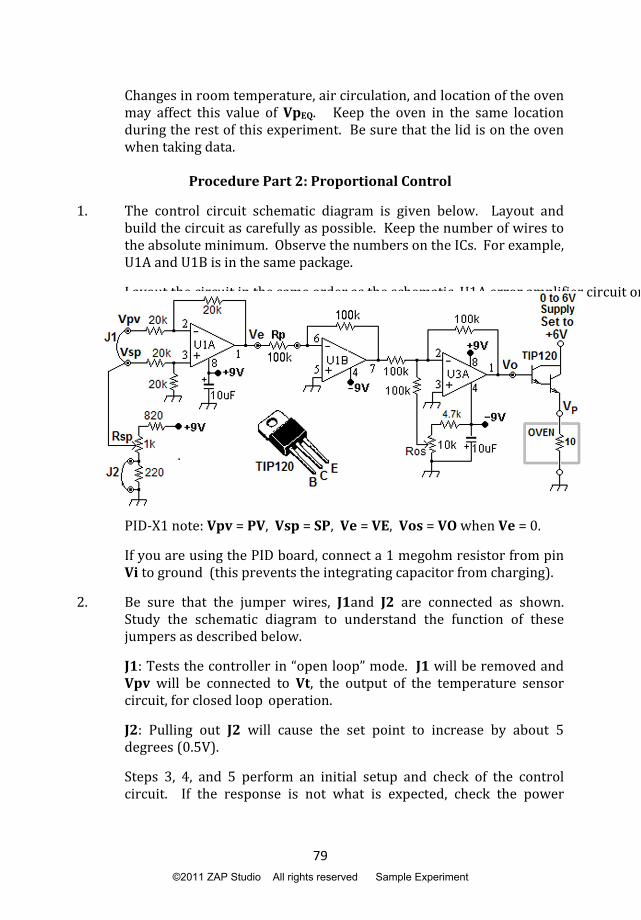
Changes in room temperature, air circulation, and location of the oven may affect this value of VpEQ. Keep the oven in the same location during the rest of this experiment. Be sure that the lid is on the oven when taking data. Procedure Part 2: Proportional Control 1. The control circuit schematic diagram is given below. Layout and build the circuit as carefully as possible. Keep the number of wires to the absolute minimum. Observe the numbers on the ICs. For example, U1A and U1B is in the same package. Layout the circuit in the same order as the schematic, U1A error amplifier circuit on

PID-X1 note: Vpv = PV, Vsp = SP, Ve = VE, Vos = VO when Ve = 0. If you are using the PID board, connect a 1 megohm resistor from pin

Vi to ground (this prevents the integrating capacitor from charging). 2. Be sure that the jumper wires, J1and J2 are connected as shown. Study the schematic diagram to understand the function of these jumpers as described below. J1: Tests the controller in “open loop” mode. J1 will be removed and Vpv will be connected to Vt, the output of the temperature sensor circuit, for closed loop operation. J2: Pulling out J2 will cause the set point to increase by about 5 degrees (0.5V). Steps 3, 4, and 5 perform an initial setup and check of the control circuit. If the response is not what is expected, check the power


80

supply connections, check the input and output voltages of the op-amps, and check the wiring carefully. 3. Apply plus and minus 9 to 12 volts to the controller and plus 6 volts to the heater circuit (TIP120 collector). Set the 0 to 6 volt supply to 6.0 volts. The temperature sensor circuit is not connected to the control circuit yet. Check that the voltage Ve is zero. Set Vp to zero with the potentiometer Req. If Vp or Ve are not zero (less than 0.1 volts), locate the problem by checking voltages at the inputs and outputs of each stage. Adjust the potentiometer, Ros, to set Vp at the emitter of the transistor to the value of VpEQ, which you measured in part 1, step 6. 4. Set the voltage Vsp with potentiometer Rsp to the voltage that represents the oven’s equilibrium temperature (TEQ from step 6 of part 1). This is the set point voltage. For example, if TEQ is 37 degrees, set Vsp to 3.7 volts. 5. Double check that Vsp is correct (set point voltage) and that Ve is zero. Turn off the 0 to 6 volt power supply

Data Logger Setup 1. Remove jumper J1 and connect Vpv to Vt (control circuit input to temperature sensor circuit output). Connect data logger channel 1 to measure Vpv (oven temperature) and connect data logger channel 2 to measure Vsp (set point temperature). Channel 1 will log the oven temperature as it approaches the set point. If more channels are available, error voltage Ve and oven voltage Vp could be logged. 2. Set the data logger to take one sample every two seconds. Set the number of samples to 400 (logging can be stopped when sufficient data is logged). 3. Connect the DMM to Vt to monitor the temperature. The oven temperature should be below 30 degrees before starting the data logger. If it is above 30 degrees take the lid off the oven and cool it with a paper fan. 4. When ready, with the lid on the oven, apply power to the oven by turning on the 0 to 6 volt power supply and start the data logger.


81

When the oven temperature stops changing (reaches equilibrium) for about 20 seconds, pull out jumper J2. This will cause the oven temperature to increase to the new set point. When the temperature stops changing, turn off the data logger and the oven power supply. 5. Cool the oven to a temperature below 30 degrees. Reconnect jumper J2. Change Rp to 20k ohms. Repeat steps 2, 3 and 4. Note: The oven temperature should reach the first set point accurately. When the jumper wire is pulled the set point is increased and the temperature will increase, but it will not reach the second set point. Step 5 increases the proportional gain so that the temperature will get closer to the second set point, but it will still not reach it. You may need to adjust your data logger timing to better match your oven’s response. You may need to check your oven equilibrium calibration and controller setup if the temperature does not reach the first set point accurately.

Analysis Write a report on this experiment. Use a word processor and cut and paste operations to transfer all relevant data and graphs to your word processor document. Include the following: 1. Introduction and objectives. 2. Data and graphs for each part. 3. Analysis of data and graphs. a) System response from room temperature to first set point. b) System response from first set point to second set point. c) Rise times, settling times, overshoot, undershoot, oscillation. d) Given that the proportional range of the heater voltage is about 0 volts to 5 volts, determine the proportional band of the control system for the error voltage, Ve, for each value of Rp. 4. Summary and conclusion.


83

Motor Speed Control The next three applications should be done sequentially, starting with application 4. All three labs require a small DC motor with an optical interrupter that produces 4 pulses per rotation. All three applications use the PID plug-in board described in Appendix 2. If the PID board is not used, the circuit may be built on a breadboard. Refer to Appendix 2 for the circuit diagram and parts information. Parts required in addition to the PID plug-in board are listed in each application. A suggested motor-tachometer assembly is described in appendix 1.

Application 4: Proportional Mode DC Motor Control Tachometer

An “optical interrupter module” and a “mono-stable multi-vibrator” (one-shot) are used to measure the rotational speed of a small DC motor. The motor’s shaft has a wheel attached which has holes or slots in it through which the light from an LED in the interrupter module can pass. Resulting light pulses are converted to voltage pulses by a photo-transistor. These pulses trigger the one-shot. Each trigger pulse causes the one-shot to produce a constant width pulse whose width is independent the trigger frequency. Since the pulse width is constant, the duty cycle at the output of the LM555 increases with frequency. This produces a voltage at the output of the low-pass filter/integrator which is proportional to the motor’s rotational speed (rpm). The output pulse width is adjusted to produce a transfer function of 1 volt per 1000 rpm of the motor. Refer to the block diagram below showing the motor and tachometer circuit connected to a PID control system. A block diagram of the motor-tachometer circuit is shown below. Potentiometer Rpw sets the output pulse width of the one-shot. It is is adjusted so that the voltage, Vpv, is equal to 1 volt per 1000 rpm. Refer to the table on the next page.


84

RPM Pulses/Min. Pulses/Sec. Period -mSec. Duty Cycle Vpv 2000 8000 133 7.5 .29 2.0 3000 12000 200 5 .43 3.0 4000 16000 267 3.75 .57 4.0 5000 20000 333 3 .71 5.0 The table above assumes that the photo-interrupter generates 4 pulses per revolution of the motor. The one-shot’s trigger pulse width must be shorter than its output pulse width. The output voltage Vpv also depends on the one-shot’s output voltage, which is about 7 volts when an 8 volt power supply is used. The values in the table assume a one-shot output voltage of 7.0 volts.

Parts and Equipment Required Dual-trace Oscilloscope, Digital Multi-meter PID-X1 controller board (or build circuit on a breadboard) Power Supply: 6 volt, 1 amp and ±12 volts, 100mA. ICs: LM555, LM358, LM78L08. Transistor: TIP120 or equiv. Resistors: 4.7K, 10k, 47k, 100k, 1/4W, 5%, 2-10K trim pots. Capacitors: 2 - 10nF, 470nF, 2-10µF electrolytic. DC Motor/Photo-interrupter. Refer to the motor set in Appendix 1.

Procedure Part 1: Tachometer Calibration 1. Connect the tachometer circuit as shown below. 2.


85

Connect a function generator to Vti set to produce a 200 Hertz, 8 volt peak-to-peak square wave, with a 20% duty cycle, and with a positive offset of 4 volts (so it goes from 0 to 8 volts). See the note below step 3. Connect oscilloscope channel 1 to pin 2 of the LM555. Connect Channel 2 to pin 3 of the LM555. Trigger on channel 1, on falling edge. Note: If you can’t vary the duty cycle of the function generator, connect the high-pass filter circuit on the right between the generator and Vti. The diode clamps the positive pulse. This produces a sharp negative pulse with a short exponential rise time. The waveforms on channels 1 and 2 should be similar to the simulated waveforms on the right. Channel 1 shows the trigger pulse applied to the trigger input. Channel 2 shows the output pulse of the LM555. You can vary the pulse width with the pot, Rpw. 4. Connect a DMM to read the DC voltage, Vpt, at pin 1 of U2. Adjust the potentiometer, Rpw, to produce exactly 3.0 volts on the DMM. 5. Measure and record the pulse amplitude in volts and the pulse width in milli-seconds of the channel 2 waveform. Amplitude (200 Hz): ___________ Pulse width (200 Hz): __________ 6. Change the function generator frequency to 267 Hertz. Verify that the DMM reads a voltage close to 4.0 volts (about ±0.1 volts). This completes the calibration of the tachometer. Disconnect the function generator.


86

Procedure Part 2: Motor Characteristics The diagram below shows the motor and photo-interrupter circuit. The motor is driven by the darlington transistor, TIP120, whose emitter voltage (and motor voltage) is controlled by the voltage applied to its base. Note that the output of the photo-interrupter is at the terminal Vt. Vt will be connected to the input, Vti, of the tachometer circuit. The 8 volt power supply for the photo-interrupter circuit is from the 8 volt regulator of the one-shot circuit. 1. Connect a the motor circuit shown above but do not connect the TIP120 emitter to the motor yet. Disconnect the function generator. Connect Vti of the tachometer circuit to Vt of the motor-generator circuit. Also connect Vs to the output of the 8 volt regulator. Be sure to run a separate ground wire from the 6 volt power supply directly to the motor ground. 2. Set Vb to zero volts with Rs. Connect the emitter of the TIP120 to the motor (Vm). 3. Connect the DMM to Vpv to measure the motor speed (1 lt/1000rpm). Adjust the potentiometer, Rs, to set the motor speed to 2000 RPM (Vr = 2.0 volts). Measure the resulting voltages Vb and Vm (by moving the DMM probe). Repeat for 3000 RPM and 4000 RPM. Record below. Speed - RPM Vb Vm 2000 3000 4000


87

Note: The motor speed will fluctuate some, but if the fluctuation is greater than 200 rpm, check the 6 volt power supply connections. Be sure to use a separate ground lead from the 6 volt power supply directly to the motor ground. We will see later that the feedback control circuit will reduce the motor speed fluctuation. Part 3: Proportional Control

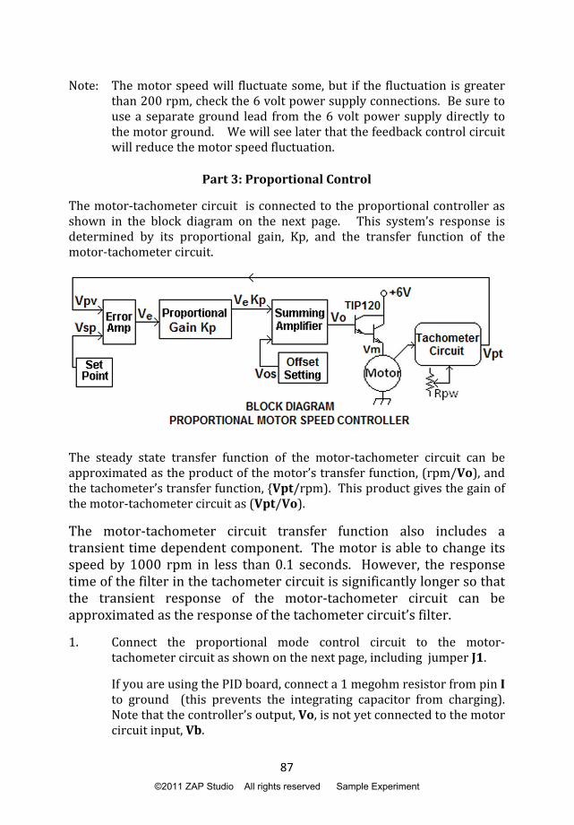
The motor-tachometer circuit is connected to the proportional controller as shown in the block diagram on the next page. This system’s response is determined by its proportional gain, Kp, and the transfer function of the motor-tachometer circuit.

The steady state transfer function of the motor-tachometer circuit can be approximated as the product of the motor’s transfer function, (rpm/Vo), and the tachometer’s transfer function, {Vpt/rpm). This product gives the gain of the motor-tachometer circuit as (Vpt/Vo). The motor-tachometer circuit transfer function also includes a transient time dependent component. The motor is able to change its speed by 1000 rpm in less than 0.1 seconds. However, the response time of the filter in the tachometer circuit is significantly longer so that the transient response of the motor-tachometer circuit can be approximated as the response of the tachometer circuit’s filter. 1. Connect the proportional mode control circuit to the motor-tachometer circuit as shown on the next page, including jumper J1. If you are using the PID board, connect a 1 megohm resistor from pin I to ground (this prevents the integrating capacitor from charging). Note that the controller’s output, Vo, is not yet connected to the motor circuit input, Vb. ©2011 ZAP Studio All rights reserved Sample Experiment

88

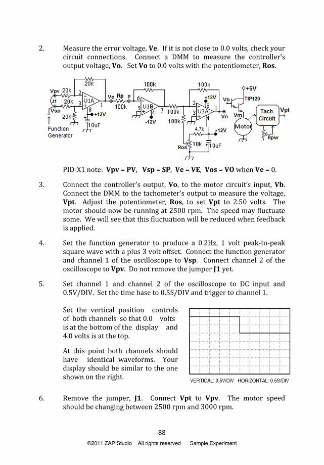
2. Measure the error voltage, Ve. If it is not close to 0.0 volts, check your circuit connections. Connect a DMM to measure the controller’s output voltage, Vo. Set Vo to 0.0 volts with the potentiometer, Ros.

PID-X1 note: Vpv = PV, Vsp = SP, Ve = VE, Vos = VO when Ve = 0. 3. Connect the controller’s output, Vo, to the motor circuit’s input, Vb. Connect the DMM to the tachometer’s output to measure the voltage, Vpt. Adjust the potentiometer, Ros, to set Vpt to 2.50 volts. The motor should now be running at 2500 rpm. The speed may fluctuate some. We will see that this fluctuation will be reduced when feedback is applied. 4. Set the function generator to produce a 0.2Hz, 1 volt peak-to-peak square wave with a plus 3 volt offset. Connect the function generator and channel 1 of the oscilloscope to Vsp. Connect channel 2 of the oscilloscope to Vpv. Do not remove the jumper J1 yet. 5. Set channel 1 and channel 2 of the oscilloscope to DC input and 0.5V/DIV. Set the time base to 0.5S/DIV and trigger to channel 1. Set the vertical position controls of both channels so that 0.0 volts is at the bottom of the display and 4.0 volts is at the top. At this point both channels should have identical waveforms. Your display should be similar to the one shown on the right. 6. Remove the jumper, J1. Connect Vpt to Vpv. The motor speed should be changing between 2500 rpm and 3000 rpm.


89

The oscilloscope display should be similar to that shown on the right. Note: Your response may vary depending on the type of motor used. Be sure that Vpv settles on 2.5 volts when Vsp = 2.5 volts. Vpv will look “fuzzy” due to the ripple from the tachometer filter. Use the average value of Vpv for your data. Record the following data for proportional gain equal to 1: Vpv rise time: ______________ Vpv fall time: ________________ Vpv high settling voltage: _______________________________ Vpv low settling voltage: ________________________________ 7. Repeat step 6 for proportional gain equal to 10 (change the value of Rp to 10k). Record the following data for proportional gain equal to 1: Vpv rise time: _______________ Vpv fall time: _______________ Vpv high settling voltage: _______________________________ Vpv low settling voltage: ________________________________ 8. Optional: Experiment with higher proportional gains. What value of gain produces the best response in terms of rise time, settling time, and proportional error?

Analysis Write a report on this experiment. Use a word processor and “cut and paste” to transfer all relevant information. Include the following: 1. Introduction and objectives. 2. Data and graphs for each part. 3. Analysis of data and graphs. 4. Summary and conclusion.


application 3: proportional mode temperature control

Documents