appendix a4: klamz model details. klamz … assessment model – technical documentation ... growth...
TRANSCRIPT

49th SAW Assessment Report Surfclam; Appendixes 193
Appendix A4: KLAMZ model details. KLAMZ Assessment Model – Technical Documentation
The KLAMZ assessment model is based on the Deriso-Schnute delay-difference equation (Deriso 1980; Schnute 1985; Quinn and Deriso 1999). The delay-difference equation is a relatively simple and implicitly age structured approach to counting fish in either numerical or biomass units. It gives the same results as explicitly age-structured models (e.g. Leslie matrix model) if fishery selectivity is “knife-edged”, if somatic growth follows the von Bertalanffy equation, and if natural mortality is the same for all age groups in each year. Knife-edge selectivity means that all individuals alive in the model during the same year experience the same fishing mortality rate.2 Natural and fishing mortality rates, growth parameters and recruitment may change from year to year, but delay-difference calculations assume that all individuals share the same mortality and growth parameters within each year. The KLAMZ model includes simple numerical models (e.g. Conser 1995) as special cases because growth can be turned off so that all calculations are in numerical units (see below).
As in many other simple models, the delay difference equation explicitly distinguishes between two age groups. In KLAMZ, the two age groups are called “new” recruits (Rt in biomass or numerical units at the beginning of year t) and “old” recruits (St) that together comprise the whole stock (Bt). New recruits are individuals that recruited at the beginning of the current year (at nominal age k).3 Old recruits are all older individuals in the stock (nominal ages k+1 and older, survivors from the previous year). As described above, KLAMZ assumes that new and old recruits are fully vulnerable to the fishery. The most important differences between the delay-difference and other simple models (e.g. Prager 1994; Conser 1995; Jacobson et al. 1994) are that von Bertalanffy growth is used to calculate biomass dynamics and that the delay-difference model captures transient age structure effects due to variation in recruitment, growth and mortality exactly. Transient effects on population dynamics are captured exactly because, as described above, the delay-difference equation is algebraically equivalent to an explicitly age-structured model with von Bertalanffy growth.
The KLAMZ model incorporates a few extensions to Schnute’s (1985) revision of Deriso’s (1980) original delay difference model. Most of the extensions facilitate tuning to a wider variety of data that anticipated in Schnute (1985). The KLAMZ model is programmed in both Excel and in C++ using AD Model Builder4 libraries. The AD Model Builder version is faster, more reliable and probably better for producing 2 In applications, assumptions about knife-edge selectivity can be relaxed by assuming the model tracks “fishable”, rather that total, biomass (NEFSC 2000a; 2000b). An analogous approach assigns pseudo-ages based on recruitment to the fishery so that new recruits in the model are all pseudo-age k. The synthetic cohort of fish pseudo-age k may consist of more than one biological cohort. The first pseudo-age (k) can be the predicted age at first, 50% or full recruitment based a von Bertalanffy curve and size composition data (Butler et al. 2002). The “incomplete recruitment” approach (Deriso 1980) calculates recruitment to the model in each year Rt as the weighted sum of contributions from two or more biological cohorts (year-
classes) from spawning during successive years (i.e.
k
aatat rR
1
where k is the age at full recruitment
to the fishery, ra is the contribution of fish age k-a to the fishable stock, and at is the number or
biomass of fish age k-a during year t). 3 In some applications, and more generally, new recruits might be defined as individuals recruiting at the beginning or at any time during the current time step (e.g. NEFSC 1996). 4 Otter Research Ltd., Box 2040, Sydney, BC, Canada V8L 3S3 ([email protected]).

49th SAW Assessment Report Surfclam; Appendixes 194
“official” stock assessment results. The Excel version is slower and implements fewer features, but the Excel version remains useful in developing prototype assessment models, teaching and for checking calculations.
The most significant disadvantage in using the KLAMZ model and other delay-difference approaches, beyond the assumption of knife-edge selectivity, is that age and length composition data are not used in tuning. However, one can argue that age composition data are used indirectly to the extent they are used to estimate growth parameters or if survey survival ratios (e.g. based on the Heinke method) are used in tuning (see below). Population dynamics
The assumed birth date and first day of the year are assumed the same in derivation of the delay-difference equation. It is therefore natural (but not strictly necessary) to tabulate catch and other data using annual accounting periods that start on the assumed biological birthday of cohorts. Biomass dynamics
As implemented in the KLAMZ model, Schnute’s (1985) delay-difference equation is:
ttt1t1-t1-tttt1t R J - R B - B ) (1 B
where Bt is total biomass of individuals at the beginning of year t; is Ford’s growth coefficient (see below); t=exp(-Zt)=exp[-(Ft+Mt)] is the fraction of the stock that survived in year t, Zt, Ft, and Mt are instantaneous rates for total, fishing and natural mortality; and Rt is the biomass of new recruits (at age k) at the beginning of the year. The natural mortality rate Mt may vary over time. Instantaneous mortality rates in KLAMZ model calculations are biomass-weighted averages if von Bertalanffy growth is turned on in the model. However, biomass-weighted mortality estimates in KLAMZ are the same as rates for numerical estimates under the assumption of knife-edge selectivity because all individuals are fully recruited. The growth parameter Jt = wt-1,k-1 / wt,k is the ratio of mean weight one year before recruitment (age k-1 in year t-1) and mean weight at recruitment (age k in year t).
It is not necessary to specify body weights at and prior to recruitment in the KLAMZ model (parameters vt-1 and Vt in Schnute 1985) because the ratio Jt and recruitment biomass contain the same information. Schnute’s (1985) original delay difference equation is:
t1-k1,-tt1tk1,t1-t1-tttt1t N - N B - B ) (1 B ww
To derive the equation used in KLAMZ, substitute recruitment biomass Rt+1 for the product wt+1,k Nt+1,k and adjusted recruitment biomass Jt Rt = (wt-1,k-1/wt,k) wt,k Nt,k = wt-1,k-1 Nt in the last term on the right hand side. The advantage in using the alternate parameterization for biomass dynamic calculations in KLAMZ is that recruitment is estimated directly in units of biomass and the number of growth parameters is reduced. The disadvantage is that numbers of recruits are not estimated directly by the model. When required, numerical recruitments must be calculated externally as the ratio of estimated recruitment biomass and the average body weight for new recruits. Numerical population dynamics

49th SAW Assessment Report Surfclam; Appendixes 195
Growth can be turned on off so that abundance, rather than biomass, is tracked in the KLAMZ model. Set Jt=1 and =0 in the delay difference equation, and use Nt (for numbers) in place of Bt to get:
1ttt1t R N N
Mathematically, the assumption Jt=1 means that no growth occurs the assumption =0 means that the von Bertalanffy K parameter is infinitely large (Schnute 1985). All tuning and population dynamics calculations in KLAMZ for biomass dynamics are also valid for numerical dynamics. Growth
As described in Schnute (1985), biomass calculations in the KLAMZ model are based on Schnute and Fournier’s (1980) re-parameterization of the von Bertalanffy growth model:
)-(1 / ) (1 ) w- (w w w k-a11-kk1-ka
where wk=V and wk-1=v. Schnute and Fournier’s (1980) growth model is the same as the traditional von Bertalanffy growth model {Wa= Wmax [1 - exp(-K(a-tzero)] where Wmax, K and tzero are parameters}. The two growth models are the same because Wmax = (wk - wk-1)/(1-), K = -ln() and tzero = ln[(wk - wk-1)/(wk - wk-1)] / ln().
In the KLAMZ model, the growth parameters Jt can vary with time but is constant. Use of time-variable Jt values with is constant is the same as assuming that the von Bertalanffy parameters Wmax and tzero change over time. Many growth patterns can be mimicked by changing Wmax and tzero (Overholtz et al., 2003). K is a parameter in the C++ version and, in principal, estimable. However, in most cases it is necessary to use external estimates of growth parameters as constants in KLAMZ. Instantaneous growth rates
Instantaneous growth rate (IGR) calculations in the KLAMZ model are an extension to the original Deriso-Schnute delay difference model. IGRs are used extensively in KLAMZ for calculating catch biomass and projecting stock biomass forward to the time at which surveys occur. The IGR for new recruits depends only on growth parameters:
)1ln(ln,
1,1t
tk
tkNewt J
w
wG
IGR for old recruits is a biomass-weighted average that depends on the current age structure and growth parameters. It can be calculated easily by projecting biomass of old recruits St=Bt-Rt (escapement) forward one year with no mortality: 11
* 1 tttt BSS
where the asterisk (*) means just prior to the start of the subsequent year t+1. By definition, the IGR for old recruits in year t is tt
Oldt SSG *ln . Dividing by St gives:
t
tt
Oldt S
BG 1
11ln
IGR for the entire stock is the biomass weighted average of the IGR values for new and old recruits:

49th SAW Assessment Report Surfclam; Appendixes 196
t
Oldtt
Newtt
t B
GSGRG
All IGR values are zero if growth is turned off. Recruitment In the Excel version of the KLAMZ model, annual recruitments are calculated
teRt where t is a log transformed annual recruitment parameter, which is estimated
in the model. In the C++ version, recruitments are calculated based on two log geometric mean recruitment parameters (, t), and a set of annual log scale deviation parameters (t): ttt
The parameter t is an offset for a step function that may be zero for all years or zero for years up to a user-specified “change year” and any value (usually estimated) afterward. The user must specify the change year, which cannot be estimated. The change year might be chosen based on auxiliary information outside the model, preliminary model fits or by carrying out a set of runs using sequential change year values and to choosing the change year that provides the best fit to the data. The deviations t are constrained to average zero.5 With the constraint, for example, estimation of and the set of t values (1+ n years parameters) is equivalent to estimation of the smaller set (n years) of t values. Natural mortality Natural mortality rates (Mt) are assumed constant in the Excel version of the KLAMZ model. In the C++ version, natural mortality rates may be estimated as a constant value or as a set of values that vary with time. In the model:
tmeMt
where m=exp() is the geometric mean natural mortality rate, is a model parameter that may be estimated (in principal but not in practical terms), and t is the log scale year-specific deviation. Deviations may be zero (turned off) so that Mt is constant, may vary in a random fashion due to auto correlated or independent process errors, or may based on a covariate.6 Model scenarios with zero recruitment may be initializing the parameter to a small value (e.g. 10-16 ) and not estimating it.
Random natural mortality process errors are effects due to predation, disease, parasitism, ocean conditions or other factors that may vary over time but are not included in the model. Calculations are basically the same as for survey process errors (see below).
Natural mortality rate covariate calculations are similar to survey covariate calculations (see below) except that the user should standardized covariates to average zero over the time period included in the model:
KKtt
5 The constraint is implemented by adding 2L (where is the average deviation) to the objective function, generally with a high weighting factor ( = 1000) so that the constraint is binding. 6 Another approach to using time dependent natural mortality rates is to treat estimates of predator consumption as discarded catch (see “Predator consumption as discard data”). In addition, estimates of predator abundance can be used in fishing effort calculations (see “Predator data as fishing effort”).

49th SAW Assessment Report Surfclam; Appendixes 197
where t is the standardized covariate, Kt is the original value, and K is the mean of the original covariate for the years in the model. Standardization to mean zero is important because otherwise m is not the geometric mean natural mortality rate (the convention is important in some calculations, see text).
Log scale deviations that represent variability around the geometric mean are calculated:
t
n
jjt p
1
where n is the number of covariates and pj is the parameter for covariate j. These conventions mean that the units for the covariate parameter pj are 1/units of the original covariate, the parameter pj measures the log scale effect of changing the covariate by one unit, and the parameter m is the log scale geometric mean. Fishing mortality and catch Fishing mortality rates (Ft) are calculated so that predicted and observed catch data (landings plus estimated discards in units of weight) “agree” to the extent specified by the user. It is not necessary, however, to assume that catches are measured accurately (see “Observed and predicted catch”).
Fishing mortality rate calculations in Schnute (1985) are exact but relating fishing mortality to catch in weight is complicated by continuous somatic growth throughout the year as fishing occurs. The KLAMZ model uses a generalized catch equation that incorporates continuous growth through the fishing season. By the definition of instantaneous rates, the catch equation expresses catch as the product:
ttt BFC ˆ
where tC is predicted catch weight (landings plus discard) and tB is average biomass.
Following Chapman (1971) and Zhang and Sullivan (1988), let Xt=Gt-Ft-Mt be the net instantaneous rate of change for biomass.7 If the rates for growth and mortality are equal, then Xt=0, tt BB and ttt BFC . If the growth rate Gt exceeds the combined
rates of natural and fishing mortality (Ft + Mt), then Xt > 0. If mortality exceeds growth, then Xt < 0. In either case, with Xt 0, average biomass is computed:
t
tX
t X
BeB
t
1
When Xt 0, the expression for tB is an approximation because Gt approximates
the rate of change in mean body weight due to von Bertalanffy growth. However, the approximation is reasonably accurate and preferable to calculating catch biomass in the delay-difference model with the traditional catch equation that ignores growth during the fishing season.8 Average biomass can be calculated for new recruits, old recruits or for the whole stock by using either New
tG , OldtG or Gt.
7 By convention, the instantaneous rates Gt, Ft and Mt are always expressed as numbers 0. 8 The traditional catch equation tt
Ztt ZBeFC t )1( where Zt=Ft+Mt underestimates catch biomass
for a given level of fishing mortality Ft and overestimates Ft for a given level of catch biomass. The errors can be substantial for fast growing fish, particularly if recent recruitments were strong.

49th SAW Assessment Report Surfclam; Appendixes 198
In the KLAMZ model, the modified catch equation may be solved analytically for Ft given Ct, Bt, Gt and Mt (see the “Calculating Ft” section below). Alternatively, fishing mortality rates can be calculated using a log geometric mean parameter () and a set of annual log scale deviation parameters (t): teFt
where the deviations t are constrained to average zero. When the catch equation is solved analytically, catches must be assumed known without error but the analytical option is useful when catch is zero or very near zero, or the range of fishing mortality rates is so large (e.g. minimum F=0.000001 to maximum F=3) that numerical problems occur with the alternative approach. The analytical approach is also useful if the user wants to reduce the number of parameters estimated by nonlinear optimization. In any case, the two methods should give the same results for catches known without error. Surplus production
Annual surplus production is calculated “exactly” by projecting biomass at the beginning of each year forward with no fishing mortality:
tt-M
1-t1-t-M
t-M*
t R J e -B L e - B e ) (1 B
By definition, surplus production Pt=B*t-Bt (Jacobson et al. 2002).
Per recruit modeling Per recruit model calculations in the Excel version of the KLAMZ simulate the life of a hypothetical cohort of arbitrary size (e.g. R=1000) starting at age k with constant Mt, F (survival) and growth ( and J) in a population initially at zero biomass. In the first year:
R B1 In the second year: 112 R J - B ) (1 B In the third and subsequent years:
1-t2
t1 B - B ) (1 B t
This iterative calculation is carried out until the sum of lifetime cohort biomass from one iteration to the next changes by less than a small amount (0.0001). Total lifetime biomass, spawning biomass and yield in weight are calculated by summing biomass, spawning biomass and yield over the lifetime of the cohort. Lifetime biomass, spawning biomass and yield per recruit are calculated by dividing totals by initial recruitment (R). Status determination variables The user may specify a range of years (e.g. the last three years) to use in calculating recent average fishing mortality centFRe and biomass centBRe levels. These
status determination variables are used in calculation of status ratios such as MSYcent FF /Re
and centBRe /BMSY.
Goodness of Fit and Parameter Estimation
Parameters estimated in the KLAMZ model are chosen to minimize an objective function based on a sum of weighted negative log likelihood (NLL) components:

49th SAW Assessment Report Surfclam; Appendixes 199
v
N
vv L
1
where NΞ is the number of NLL components (Lv) and the v are emphasis factors used as weights. The objective function may be viewed as a NLL or a negative log posterior (NLP) distribution, depending on the nature of the individual Lv components and modeling approach. Except during sensitivity analyses, weighting factors for objective function components (v) are usually set to one. An arbitrarily large weighting factor (e.g. v =1000) is used for “hard” constraints that must be satisfied in the model. Arbitrarily small weighting factors (e.g. v =0.0001) can be used for “soft” model-based constraints. For example, an internally estimated spawner-recruit curve or surplus production curve might be estimated with a small weighting factor to summarize stock-recruit or surplus production results with minimal influence on biomass, fishing mortality and other estimates from the model. Use of a small weighting factor for an internally estimated surplus production or stock-recruit curve is equivalent to fitting a curve to model estimates of biomass and recruitment or surplus production in the output file, after the model is fit (Jacobson et al. 2002). Likelihood component weights vs. observation-specific weights Likelihood component weights (v) apply to entire NLL components. Entire components are often computed as the sum of a number of individual NLL terms. The NLL for an entire survey, for example, is composed of NLL terms for each of the annual survey observations. In KLAMZ, observation-specific (for data) or instance-specific (for constraints or prior information) weights (usually wj for observation or instance j) can be specified as well. Observation-specific weights for a survey, for example, might be use to increase or decrease the importance of one or more observations in calculating goodness of fit. NLL kernels NLL components in KLAMZ are generally programmed as “concentrated likelihoods” to avoid calculation of values that do not affect derivatives of the objective function.9 For x~N(,2), the complete NLL for one observation is:
2
5.02lnln
uxL
The constant 2ln can always be omitted because it does not affect derivatives. If the
standard deviation is known or assumed known, then ln() can be omitted as well because it is a constant that does not affect derivatives. In such cases, the concentrated negative log likelihood is:
2
5.0
x
L
9 Unfortunately, concentrated likelihood calculations cannot be used with MCMC and other Bayesian approaches to characterizing posterior distributions. Therefore, in the near future, concentrated NLL calculations will be replaced by calculations for the entire NLL. At present, MCMC calculations in KLAMZ are not useful.

49th SAW Assessment Report Surfclam; Appendixes 200
If there are N observations with possible different variances (known or assumed known) and possibly different expected values:
N
i i
iixL
1
2
5.0
If the standard deviation for a normally distributed quantity is not known and is
(in effect) estimated by the model, then one of two equivalent calculations is used. Both approaches assume that all observations have the same variance and standard deviation. The first approach is used when all observations have the same weight in the likelihood:
N
ii uxNL
1
2ln5.0
where N is the number of observations. The second approach is equivalent but used when the weights for each observation (wi) may differ:
N
i
ii
uxwL
1
2
5.0ln
In the latter case, the maximum likelihood estimator:
N
xxN
ii
2
1
ˆˆ
(where x is the average or predicted value from the model) is used for . The maximum likelihood estimator is biased by N/(N-df) where df is degrees of freedom for the model. The bias may be significant for small sample sizes but df is usually unknown. Landings, discards, catch
Discards are from external estimates (dt) supplied by the user. If dt 0, then the data are used as the ratio of discard to landed catch so that:
ttt LD
where t =Dt/Lt is the discard ratio. If dt < 0 then the data are treated as discard in units
of weight: .tt dabsD
In either case, total catch is the sum of discards and landed catch (Ct = Lt + Dt). It is possible to use discards in weight dt < 0 for some years and discard as proportions dt > 0 for other years in the same model run. If catches are estimated (see below) so that the
estimated catch tC does not necessarily equal observed landings plus discard, then
estimated landings are computed:
t
tt
CL
1
ˆˆ
and estimated discards are:
.ˆˆttt LD
49th SAW Assessment Report Surfclam; Appendixes 201
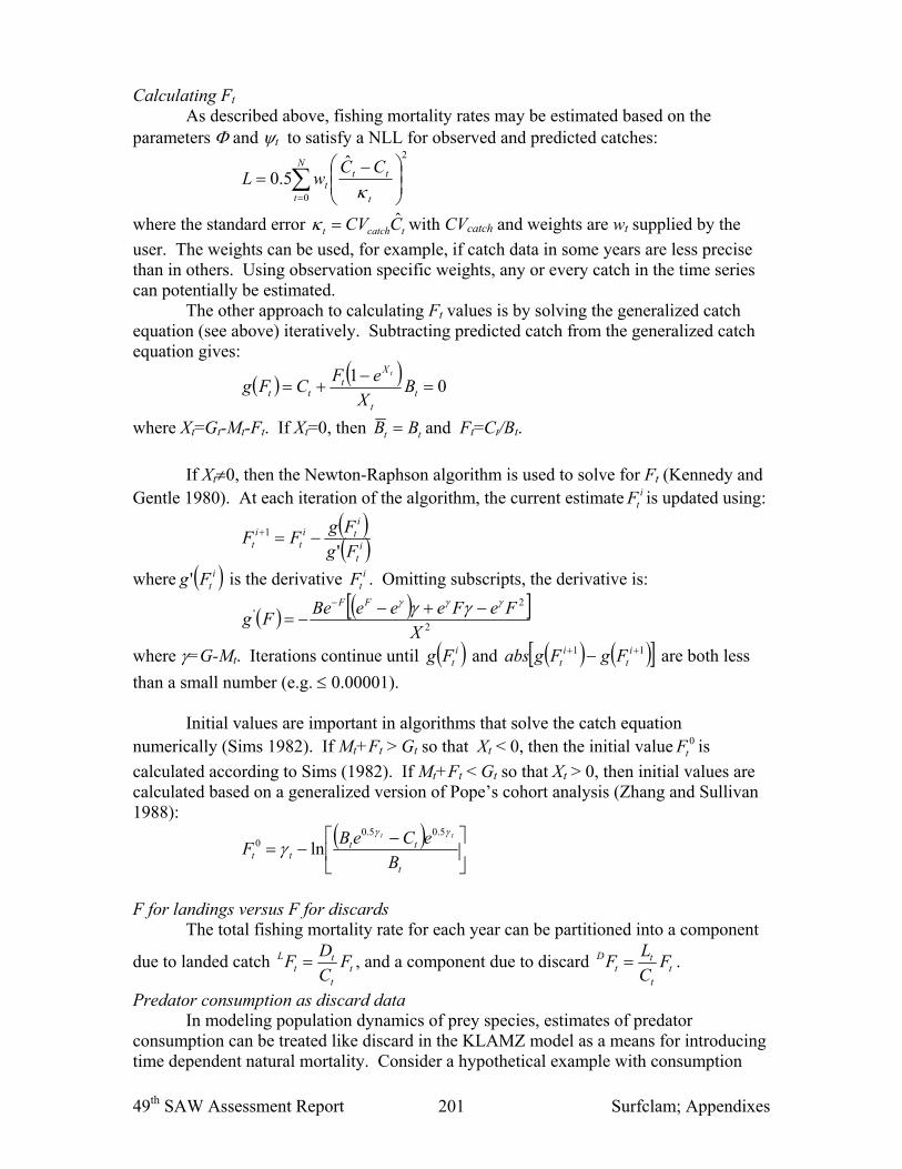
Calculating Ft As described above, fishing mortality rates may be estimated based on the
parameters and t to satisfy a NLL for observed and predicted catches:
2
0
ˆ5.0
N
t t
ttt
CCwL
where the standard error tcatcht CCV ˆ with CVcatch and weights are wt supplied by the
user. The weights can be used, for example, if catch data in some years are less precise than in others. Using observation specific weights, any or every catch in the time series can potentially be estimated.
The other approach to calculating Ft values is by solving the generalized catch equation (see above) iteratively. Subtracting predicted catch from the generalized catch equation gives:
0
1
t
t
Xt
tt BX
eFCFg
t
where Xt=Gt-Mt-Ft. If Xt=0, then tt BB and Ft=Ct/Bt.
If Xt0, then the Newton-Raphson algorithm is used to solve for Ft (Kennedy and
Gentle 1980). At each iteration of the algorithm, the current estimate itF is updated using:
it
iti
ti
t Fg
FgFF
'1
where itFg ' is the derivative itF . Omitting subscripts, the derivative is:
2
2'
X
FeFeeeBeFg
FF
where =G-Mt. Iterations continue until itFg and 11 it
it FgFgabs are both less
than a small number (e.g. 0.00001).
Initial values are important in algorithms that solve the catch equation numerically (Sims 1982). If Mt+Ft > Gt so that Xt < 0, then the initial value 0
tF is
calculated according to Sims (1982). If Mt+Ft < Gt so that Xt > 0, then initial values are calculated based on a generalized version of Pope’s cohort analysis (Zhang and Sullivan 1988):
t
tttt B
eCeBF
tt
5.05.0
0 ln
F for landings versus F for discards The total fishing mortality rate for each year can be partitioned into a component
due to landed catch tt
tt
L FC
DF , and a component due to discard t
t
tt
D FC
LF .
Predator consumption as discard data In modeling population dynamics of prey species, estimates of predator consumption can be treated like discard in the KLAMZ model as a means for introducing time dependent natural mortality. Consider a hypothetical example with consumption

49th SAW Assessment Report Surfclam; Appendixes 202
data (mt y-1) for three important predators. If the aggregate consumption data are included in the model as “discards”, then the fishing mortality rate for discards dFt (see above) would be an estimate of the component of natural mortality due to the three predators. In using this approach, the average level of natural mortality m would normally be reduced (e.g. so that old
dnew mFm ) or estimated to account for the portion
of natural mortality attributed to bycatch. Surplus production calculations are harder to interpret if predator consumption is treated as discard data because surplus production calculations assume that Ft=0 (see above) and because surplus production is defined as the change in biomass from one year to the next in the absence of fishing (i.e. no landings or bycatch). However, it may be useful to compare surplus production at a given level of biomass from runs with and without consumption data as a means of estimating maximum changes in potential fishery yield if the selected predators were eliminated (assuming no change in disease, growth rates, predation by other predators, etc.). Effort calculations Fishing mortality rates can be tuned to fishing effort data for the “landed” catch (i.e. excluding discards). Years with non-zero fishing effort used in the model must also have landings greater than zero. Assuming that effort data are lognormally distributed, the NLL for fishing effort is:
effn
y
yyy
EEwNLL
1
2ˆln5.0
where wy is an observation-specific weight, neff is the number of active effort observations (i.e. with wy > 0), Ey and yE are observed and predicted fishing effort data, and the log
scale variance is a constant calculated from a user-specified CV. Predicted fishing effort data are calculated:
yy FE ˆ
where =eu, =eb, and u and b are parameters estimated by the model. If the parameter
b is not estimated, then =1 so that the relationship between fishing effort and fishing mortality is linear. If the parameter b is estimated, then 1 and the relationship is a power function. Predator data as fishing effort As described under “Predator consumption as discard data”, predator consumption data can be treated as discard. If predator abundance data are available as well, and assuming that mortality due predators is a linear function of the predator-prey ratio, then both types of data may be used together to estimate natural mortality. The trick is to: 1) enter the predator abundance data as fishing effort; 2) enter the actual fishery landings as “discard”; 3) enter predator consumption estimates of the prey species as “landings” so that the fishing effort data in the refer to the predator consumption data; 4) use an option in the model to calculate the predator-prey ratio for use in place of the original predator abundance “fishing effort” data; and 5) tune fishing mortality rates for landings (a.k.a. predator consumption) to fishing effort (a.k.a. predator-prey ratio).

49th SAW Assessment Report Surfclam; Appendixes 203
Given the predator abundance data y , the model calculates the predator-prey
ratio used in place of fishing effort data (Ey) as:
y
yy B
E
where By is the model’s current estimate of total (a.k.a “prey”) biomass. Subsequent calculations with Ey and the model’s estimates of “fishing mortality” (Fy, really a measure of natural mortality) are exactly as described above for effort data. In using this approach, it is probably advisable to reduce m (the estimate of average mortality in the model) to account for the proportion of natural mortality due to predators included in the calculation. Based on experience to date, natural mortality due to consumption by the suite of predators can be estimated but only if m is assumed known. Initial population age structure
In the KLAMZ model, old and new recruit biomass during the first year (R1 and S1 =B1-R1) and biomass prior to the first year (B0) are estimated as log scale parameters. Survival in the year prior to the first year (“year 0”) is 10
0MFe with F0 chosen to
obtain catch C0 (specified as data) from the estimated biomass B0. IGRs during year 0 and year 1 are assumed equal (G0=G1) in catch calculations.
Biomass in the second year of as series of delay-difference calculations depends on biomass (B0) and survival (0) in year 0:
1112001112 R J - R B - B ) (1 B
There is, however, there is no direct linkage between B0 and escapement biomass (S1=B1-R1) at the beginning of the first year.
The missing link between B0, S1 and B1 means that the parameter for B0 tends to be relatively free and unconstrained by the underlying population dynamics model. In some cases, B0 can be estimated to give good fit to survey and other data, while implying unreasonable initial age composition and surplus production levels. In other cases, B0 estimates can be unrealistically high or low implying, for example, unreasonably high or low recruitment in the first year of the model (R1). Problems arise because many different combinations of values for R1, S1 and B0 give similar results in terms of goodness of fit. This issue is common in stock assessment models that use forward simulation calculations because initial age composition is difficult to estimate. It may be exacerbated in delay-difference models because age composition data are not used.
The KLAMZ model uses two constraints to help estimate initial population biomass and initial age structure.10 The first constraint links IGRs for escapement (GOld) in the first years to a subsequent value. The purpose of the constraint is to ensure consistency in average growth rates (and implicit age structure) during the first few years. For example, if IGRs for the first nG years are constrained11, then the NLL for the penalty is:
G
G
n
t G
Oldn
Oldt
G
GGL
1
2
1ln5.0
where the standard deviation G is supplied by the user. It is usually possible to use the standard deviation of Old
tQ for later years from a preliminary run to estimate G for the
10 Quinn and Deriso (1999) describe another approach attributed to a manuscript by C. Walters. 11 Normally, nG 2.
49th SAW Assessment Report Surfclam; Appendixes 204
first few years. The constraint on initial IGRs should probably be “soft” and non-binding (1) because there is substantial natural variation in somatic growth rates due to variation in age composition.
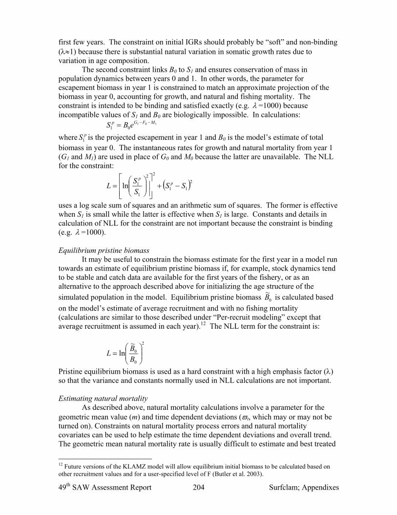
The second constraint links B0 to S1 and ensures conservation of mass in population dynamics between years 0 and 1. In other words, the parameter for escapement biomass in year 1 is constrained to match an approximate projection of the biomass in year 0, accounting for growth, and natural and fishing mortality. The constraint is intended to be binding and satisfied exactly (e.g. =1000) because incompatible values of S1 and B0 are biologically impossible. In calculations:
10101
MFGp eBS
where pS1 is the projected escapement in year 1 and B0 is the model’s estimate of total biomass in year 0. The instantaneous rates for growth and natural mortality from year 1 (G1 and M1) are used in place of G0 and M0 because the latter are unavailable. The NLL for the constraint:
211
22
1
1ln SSS
SL p
p
uses a log scale sum of squares and an arithmetic sum of squares. The former is effective when S1 is small while the latter is effective when S1 is large. Constants and details in calculation of NLL for the constraint are not important because the constraint is binding (e.g. =1000). Equilibrium pristine biomass It may be useful to constrain the biomass estimate for the first year in a model run towards an estimate of equilibrium pristine biomass if, for example, stock dynamics tend to be stable and catch data are available for the first years of the fishery, or as an alternative to the approach described above for initializing the age structure of the
simulated population in the model. Equilibrium pristine biomass 0
~B is calculated based
on the model’s estimate of average recruitment and with no fishing mortality (calculations are similar to those described under “Per-recruit modeling” except that average recruitment is assumed in each year).12 The NLL term for the constraint is:
2
0
0
~ln
B
BL
Pristine equilibrium biomass is used as a hard constraint with a high emphasis factor () so that the variance and constants normally used in NLL calculations are not important. Estimating natural mortality As described above, natural mortality calculations involve a parameter for the geometric mean value (m) and time dependent deviations (t, which may or may not be turned on). Constraints on natural mortality process errors and natural mortality covariates can be used to help estimate the time dependent deviations and overall trend. The geometric mean natural mortality rate is usually difficult to estimate and best treated
12 Future versions of the KLAMZ model will allow equilibrium initial biomass to be calculated based on other recruitment values and for a user-specified level of F (Butler et al. 2003).
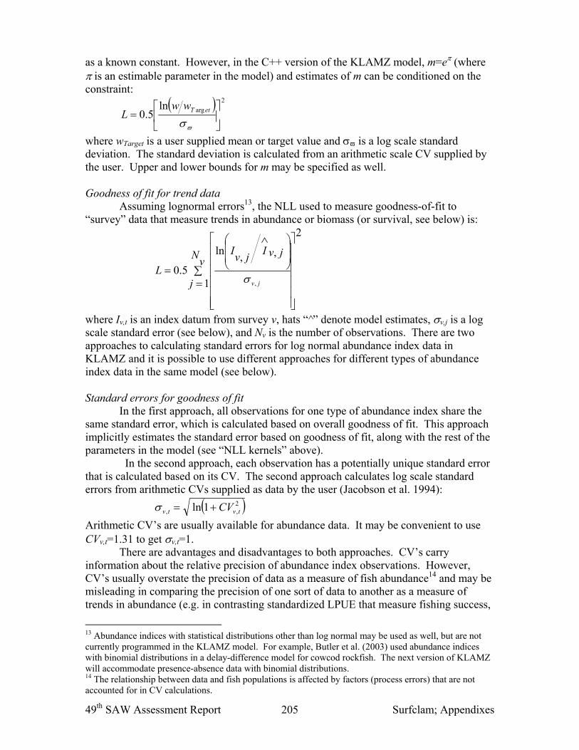
49th SAW Assessment Report Surfclam; Appendixes 205
as a known constant. However, in the C++ version of the KLAMZ model, m=e (where is an estimable parameter in the model) and estimates of m can be conditioned on the constraint:
2
argln5.0
etTww
L
where wTarget is a user supplied mean or target value and is a log scale standard deviation. The standard deviation is calculated from an arithmetic scale CV supplied by the user. Upper and lower bounds for m may be specified as well. Goodness of fit for trend data
Assuming lognormal errors13, the NLL used to measure goodness-of-fit to “survey” data that measure trends in abundance or biomass (or survival, see below) is:
v
N
j
jvIjv
I
Ljv1
2
,,ln
5.0,
where Iv,t is an index datum from survey v, hats “^” denote model estimates, v,j is a log scale standard error (see below), and Nv is the number of observations. There are two approaches to calculating standard errors for log normal abundance index data in KLAMZ and it is possible to use different approaches for different types of abundance index data in the same model (see below). Standard errors for goodness of fit
In the first approach, all observations for one type of abundance index share the same standard error, which is calculated based on overall goodness of fit. This approach implicitly estimates the standard error based on goodness of fit, along with the rest of the parameters in the model (see “NLL kernels” above).
In the second approach, each observation has a potentially unique standard error that is calculated based on its CV. The second approach calculates log scale standard errors from arithmetic CVs supplied as data by the user (Jacobson et al. 1994):
2,, 1ln tvtv CV
Arithmetic CV’s are usually available for abundance data. It may be convenient to use CVv,t=1.31 to get v,t=1.
There are advantages and disadvantages to both approaches. CV’s carry information about the relative precision of abundance index observations. However, CV’s usually overstate the precision of data as a measure of fish abundance14 and may be misleading in comparing the precision of one sort of data to another as a measure of trends in abundance (e.g. in contrasting standardized LPUE that measure fishing success,
13 Abundance indices with statistical distributions other than log normal may be used as well, but are not currently programmed in the KLAMZ model. For example, Butler et al. (2003) used abundance indices with binomial distributions in a delay-difference model for cowcod rockfish. The next version of KLAMZ will accommodate presence-absence data with binomial distributions. 14 The relationship between data and fish populations is affected by factors (process errors) that are not accounted for in CV calculations.
49th SAW Assessment Report Surfclam; Appendixes 206
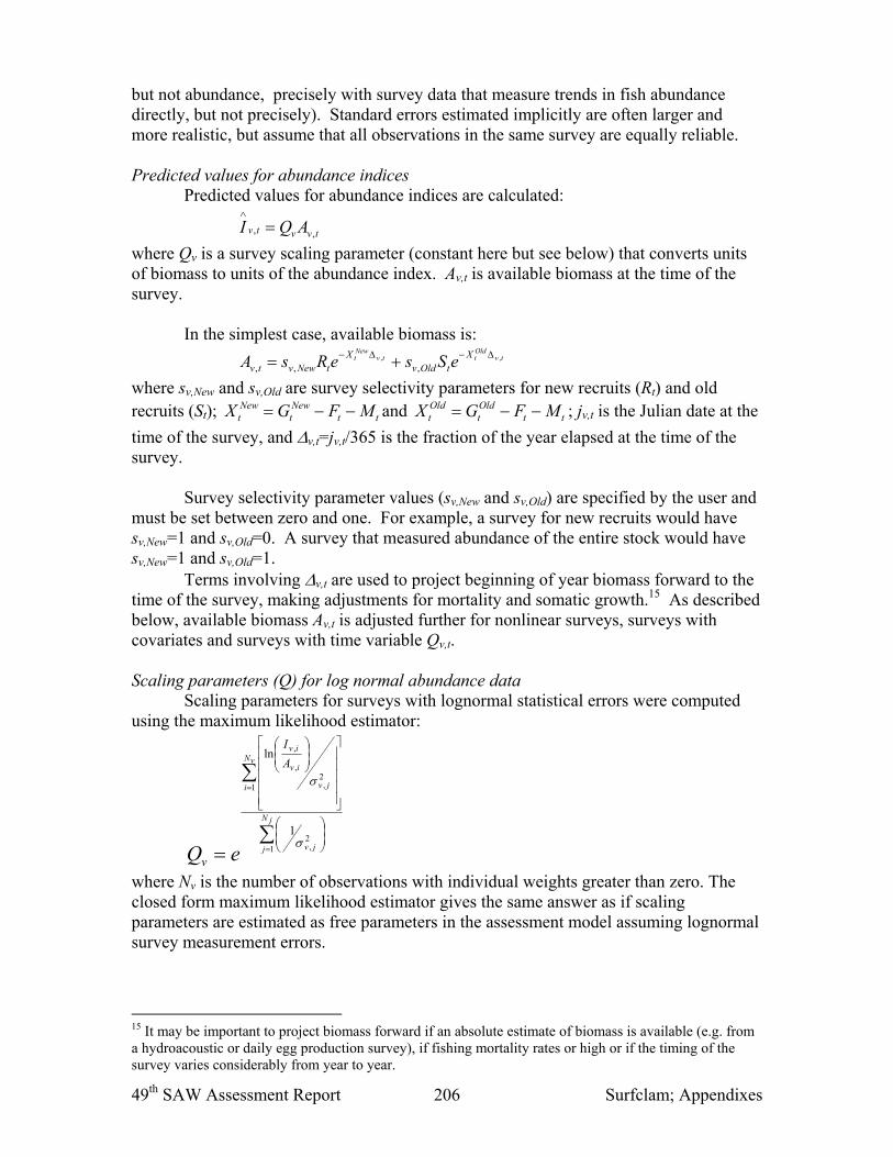
but not abundance, precisely with survey data that measure trends in fish abundance directly, but not precisely). Standard errors estimated implicitly are often larger and more realistic, but assume that all observations in the same survey are equally reliable. Predicted values for abundance indices
Predicted values for abundance indices are calculated:
tvvtv AQI ,,
where Qv is a survey scaling parameter (constant here but see below) that converts units of biomass to units of the abundance index. Av,t is available biomass at the time of the survey.
In the simplest case, available biomass is:
tvOldttv
Newt X
tOldvX
tNewvtv eSseRsA ,,
,,,
where sv,New and sv,Old are survey selectivity parameters for new recruits (Rt) and old recruits (St); tt
Newt
Newt MFGX and tt
Oldt
Oldt MFGX ; jv,t is the Julian date at the
time of the survey, and v,t=jv,t/365 is the fraction of the year elapsed at the time of the survey.
Survey selectivity parameter values (sv,New and sv,Old) are specified by the user and
must be set between zero and one. For example, a survey for new recruits would have sv,New=1 and sv,Old=0. A survey that measured abundance of the entire stock would have sv,New=1 and sv,Old=1.
Terms involving v,t are used to project beginning of year biomass forward to the time of the survey, making adjustments for mortality and somatic growth.15 As described below, available biomass Av,t is adjusted further for nonlinear surveys, surveys with covariates and surveys with time variable Qv,t.
Scaling parameters (Q) for log normal abundance data
Scaling parameters for surveys with lognormal statistical errors were computed using the maximum likelihood estimator:
jN
j jv
vN
i jv
iv
iv
A
I
v eQ 12,
12,
,
,
1
ln
where Nv is the number of observations with individual weights greater than zero. The closed form maximum likelihood estimator gives the same answer as if scaling parameters are estimated as free parameters in the assessment model assuming lognormal survey measurement errors.
15 It may be important to project biomass forward if an absolute estimate of biomass is available (e.g. from a hydroacoustic or daily egg production survey), if fishing mortality rates or high or if the timing of the survey varies considerably from year to year.
49th SAW Assessment Report Surfclam; Appendixes 207
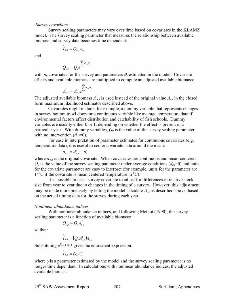
Survey covariates Survey scaling parameters may vary over time based on covariates in the KLAMZ model. The survey scaling parameter that measures the relationship between available biomass and survey data becomes time dependent:
tvtvtv AQI ,,,
and
vn
rrtrd
vtv eQQ 1,
,
with nv covariates for the survey and parameters r estimated in the model. Covariate effects and available biomass are multiplied to compute an adjusted available biomass:
vn
rrtrd
tvtv eAA 1,
,,
The adjusted available biomass A’v,t is used instead of the original value Av,t in the closed
form maximum likelihood estimator described above. Covariates might include, for example, a dummy variable that represents changes
in survey bottom trawl doors or a continuous variable like average temperature data if environmental factors affect distribution and catchability of fish schools. Dummy variables are usually either 0 or 1, depending on whether the effect is present in a particular year. With dummy variables, Qv is the value of the survey scaling parameter with no intervention (dr,t=0).
For ease in interpretation of parameter estimates for continuous covariates (e.g. temperature data), it is useful to center covariate data around the mean: rtrtr ddd ,,
where d’r,t is the original covariate. When covariates are continuous and mean-centered,
Qv is the value of the survey scaling parameter under average conditions (dr,t=0) and units for the covariate parameter are easy to interpret (for example, units for the parameter are 1/ oC if the covariate is mean centered temperature in oC).
It is possible to use a survey covariate to adjust for differences in relative stock size from year to year due to changes in the timing of a survey. However, this adjustment may be made more precisely by letting the model calculate v,t as described above, based on the actual timing data for the survey during each year. Nonlinear abundance indices With nonlinear abundance indices, and following Methot (1990), the survey scaling parameter is a function of available biomass: tvvtv AQQ ,,
so that:
tvtvvtv AAQI ,,,
Substituting e=+1 gives the equivalent expression:
etvvtv AQI ,,
where is a parameter estimated by the model and the survey scaling parameter is no longer time dependent. In calculations with nonlinear abundance indices, the adjusted available biomass:

49th SAW Assessment Report Surfclam; Appendixes 208
etvtv AA ,,
is computed first and used in the closed form maximum likelihood estimator described above to calculate the survey scaling parameter. In cases where survey covariates are also applied to a nonlinear index, the adjustment for nonlinearity is carried out first. Survey Q process errors The C++ version of the KLAMZ model can be used to allow survey scaling parameters to change in a controlled fashion from year to year (NEFSC 2002):
tveQQ vtv,
,
where the deviations tv, are constrained to average zero. Variation in survey Q values is
controlled by the NLL penalty:
vN
jL
v
jv
1
25.0 ,
where the log scale standard deviation v based on an arithmetic CV supplied by the user (e.g. see NEFSC 2002). In practice, the user increases or decreases the amount of variability in Q by decreasing or increasing the assumed CV. Survival ratios as surveys In the C++ version of KLAMZ, it is possible to use time series of survival data as “surveys”. For example, an index of survival might be calculated using survey data and the Heinke method (Ricker 1975) as:
tk
tkt I
IA
,
1,1
so that the time series of At estimates are data that may potentially contain information about scale or trends in survival. Predicted values for an a survival index are calculated:
tZt eA ˆ
After predicted values are calculated, survival ratio data are treated in the same
way as abundance data (in particular, measurement errors are assumed to be lognormal). Selectivity parameters are ignored for survival data but all other features (e.g. covariates, nonlinear scaling relationships and constraints on Q) are available. Recruitment models Recruitment parameters in KLAMZ may be freely estimated or estimated around an internal recruitment model, possibly involving spawning biomass. An internally estimated recruitment model can be used to reduce variability in recruitment estimates (often necessary if data are limited), to summarize stock-recruit relationships, or to make use of information about recruitment in similar stocks. There are four types of internally estimated recruitment models in KLAMZ: 1) random (white noise) variation around a constant or time dependent mean modeled as a step function; 2) random walk (autocorrelated) variation around a constant or time dependent mean modeled as a step function; 3) random variation around a Beverton-Holt recruitment model; and 4) random variation around a Ricker recruitment model. The user must specify a type of recruitment

49th SAW Assessment Report Surfclam; Appendixes 209
model but the model is not active unless the likelihood component for the recruitment model is turned on ( 0 ). The first step in recruit modeling is to calculate the expected log recruitment level E[ln(Rt)] given the recruitment model. For random variation around a constant mean, the expected log recruitment level is the log geometric mean recruitment:
NRREN
jjt
1
lnln
For a random walk around a constant mean recruitment, the expected log recruitment level is the logarithm of recruitment during the previous year:
1lnln tt RRE
with no constraint on recruitment during the first year R1.
For the Beverton-Holt recruitment model, the expected log recruitment level is: t
bt
at TeTeRE lnln
where a=e and b=e, the parameters and are estimated in the model, Tt is
spawning biomass, and is the lag between spawning and recruitment. Spawner-recruit parameters are estimated as log transformed values (e and e) to enhance model stability and ensure the correct sign of values used in calculations. Spawning biomass is: toldtnewt SmRmT
where mnew and mold are maturity parameters for new and old recruits specified by the user. For the Ricker recruitment model, the expected log recruitment level is:
tbSa
tt eSRE lnln
where a=e and b=e, and the parameters and are estimated in the model.
Given the expected log recruitment level, log scale residuals for the recruitment model are calculated: ttt RERr lnln
Assuming that residuals are log normal, the NLL for recruitment residuals is:
N
tt r
trt
first
rwL2
5.0ln
where t is an instance-specific weight usually set equal one. The additional term in the NLL [ln(r)] is necessary because the variance 2
r is estimated internally, rather than specified by the user.
The log scale variance for residuals is calculated using the maximum likelihood estimator:
N
rN
tjj
rfirst
2
where N is the number of residuals. For the recruitment model with constant variation around a mean value, tfirst=1. For the random walk recruitment model, tfirst=2. For the Beverton-Holt and Ricker models, tfirst= 1 and the recruit model imposes no constraint on variability of recruitment during years 1 to (see below). The biased maximum likelihood estimate for 2 (with N in the divisor instead of the degrees of freedom) is used

49th SAW Assessment Report Surfclam; Appendixes 210
because actual degrees of freedom are unknown. The variance term 2 is calculated explicitly and stored because it is used below. Constraining the first few recruitments It may be useful to constrain the first years of recruitments when using either the Beverton-Holt or Ricker models if the unconstrained estimates for early years are erratic. In the KLAMZ model, this constraint is calculated:
1
1
2ln
5.0ln(first
first
t
t r
tt
rt
RERwNLL
where tfirst is the first year for which expected recruitment E(Rl) can be calculated with the spawner-recruit model. In effect, recruitments that not included in spawner-recruit calculations are constrained towards the first spawner-recruit prediction. The standard deviation is the same as used in calculating the NLL for the recruitment model. Prior information about the absolute value abundance index scaling parameters (Q) A constraint on the absolute value one or more scaling parameters (Qv) for abundance or survival indices may be useful if prior information is available (e.g. NEFSC 2000; NEFSC 2001; NEFSC 2002). In the Excel version, it is easy to program these (and other) constraints in an ad-hoc fashion as they are needed. In the AD Model Builder version, log normal and beta distributions are preprogrammed for use in specifying prior information about Qv for any abundance or survival index.
The user must specify which surveys have prior distributions, minimum and maximum legal bounds (qmin and qmax), the arithmetic mean q and the arithmetic CV for the prior the distribution. Goodness of fit for Qv values outside the bounds (qmin, qmax) are calculated:
min
2min
max2
max
10000
10000
qQifQq
qQifqQL
vv
vv
Goodness of fit for Qv values inside the legal bounds depend on whether the distribution of potential values is log normal or follows a beta distribution. Lognormal case
Goodness of fit for lognormal Qv values within legal bounds is:
2
ln5.0
vQ
L
where the log scale standard deviation CV 1ln and 2
ln2 q is the mean
of the corresponding log normal distribution. Beta distribution case The first step in calculation goodness of fit for Qv values with beta distributions is to calculate the mean and variance of the corresponding “standardized” beta distribution:
D
qqq min
and

49th SAW Assessment Report Surfclam; Appendixes 211
2
D
CVqqVar
where the range of the standardized beta distribution is D=qmax-qmin. Equating the mean and variance to the estimators for the mean and variance for the standardized beta distribution (the “method of moments”) gives the simultaneous equations:
ba
aq
and
)1(
' 2
baba
abqVar
where a and b are parameters of the standardized beta distribution.16 Solving the simultaneous equations gives:
qVar
qqqVarqb
11
and:
q
qba
1
Goodness of fit for beta Qv values within legal bounds is calculated with the NLL: )'1ln(1'ln1 vv QbQaL
where minqQQQ vvv is the standardized value of the survey scaling parameter Qv.
Prior information about relative abundance index scaling parameters (Q-ratios) Constraints on “Q-ratios” can be used in fitting models if some information about the relative values of scaling parameters for two abundance indices is available. For example, ASMFC (2001, p. 46-47) assumed that the relative scaling parameters for recruit and post-recruit lobsters taken in the same survey was either 0.5 or 1. If both indices are from the same survey cruise (e.g. one index for new recruits and one index for old recruits in the same survey), then assumptions about q-ratios are analogous to assumptions about the average selectivity of the survey of the survey for new and old recruits.
Q-ratio constraints tend to stabilize and have strong effects on model estimates. ASMFC (2001, p. 274) found, for example, that goodness of fit to survey data, abundance and fishing mortality estimates for lobster changed dramatically over a range of assumed q-ratio values.
To use q-ratio information in the KLAMZ model, the user must identify two surveys, a target value for the ratio of their Q values, and a CV for differences between the models estimated q-ratio and the target value. For example, if the user believes that the scaling parameters for abundance index 1 and abundance index 3 is 0.5, with a CV=0.25 for uncertainty in the prior information then the model’s estimate of the q-ratio is =Q1/Q3. The goodness of fit calculation is:
16 If x has a standardized beta distribution with parameters a and b, then the probability of x is
ba
xxxP
ba
,
1 11
.

49th SAW Assessment Report Surfclam; Appendixes 212
2
ln5.0
L
where is the target value and the log scale standard deviation is calculated from the arithmetic CV supplied by the user.
Normally, a single q-ratio constraint would be used for the ratio of new and old recruits taken during the same survey operation. However, in KLAMZ any number of q-ratio constraints can be used simultaneously and the scaling parameters can be for any two indices in the model. Surplus production modeling
Surplus production models can be fit internally to biomass and surplus production estimates in the model (Jacobson et al. 2002). Models fit internally can be used to constrain estimates of biomass and recruitment, to summarize results in terms of surplus production, or as a source of information in tuning the model. The NLL for goodness of fit assumes normally distributed process errors in the surplus production process:
PN
j
Pj
PL
j
1
2~
5.0
where Np is the number of surplus production estimates (number of years less one), tP~
is
a predicted value from the surplus production curve, Pt is the assessment model estimate, and the standard deviation is supplied by the user based, for example, on preliminary variances for surplus production estimates.17 Either the symmetrical Schaefer (1957) or
asymmetric Fox (1970) surplus production curve may be used to calculate tP~
(Quinn and
Deriso 1999). It may be important to use a surplus production curve that is compatible with
recruitment patterns or assumptions about the underlying spawner-recruit relationship. More research is required, but the asymmetric shape of the Fox surplus production curve appears reasonably compatible with the assumption that recruitment follows a Beverton-Holt spawner-recruit curve (Mohn and Black 1998). In contrast, the symmetric Schaefer surplus production model appears reasonably compatible with the assumption that recruitment follows a Ricker spawner-recruit curve.
The Schaefer model has two log transformed parameters that are estimated in KLAMZ:
2~ttt BeBeP
The Fox model also has two log transformed parameters:
e
B
e
BeeP tte
t log~
See Quinn and Deriso (1999) for formulas used to calculate reference points (FMSY, BMSY, MSY, and K) for both surplus production models. 17 Variances in NLL for surplus production-biomass models are a subject of ongoing research. The advantage in assuming normal errors is that negative production values (which occur in many stocks, e.g. Jacobson et al. 2001) are accommodated. In addition, production models can be fit easily by linear regression of Pt on Bt and Bt
2 with no intercept term. However, variance of production estimate residuals increases with predicted surplus production. Therefore, the current approach to fitting production curves in KLAMZ is not completely satisfactory.

49th SAW Assessment Report Surfclam; Appendixes 213
Catch/biomass
Forward simulation models like KLAMZ may tend to estimate absurdly high fishing mortality rates, particularly if data are limited. The likelihood constraint used to prevent this potential problem is:
N
tt qdL
0
225.0
where:
otherwise
FtifFtdt 0
and with the threshold value normally set by the user to about 0.95. Values for can be linked to maximum F values using the modified catch equation described above. For example, to use a maximum fishing mortality rate of about F4 with M=0.2 and G=0.1 (maximum X=4+0.2-0.1=4.1), set F/X(1-e-X)=4 / 4.1 (1-e-4)=0.96. Uncertainty
The AD Model Builder version of the KLAMZ model automatically calculates variances for parameters and quantities of interest (e.g. Rt, Ft, Bt, FMSY, BMSY, centFRe ,
centBRe , MSYcent FF /Re , MSYcent BB /Re , etc.) by the delta method using exact derivatives. If
the objective function is the log of a proper posterior distribution, then Markov Chain Monte Carlo (MCMC) techniques implemented in AD Model Builder libraries can be used estimate posterior distributions representing uncertainty in the same parameters and quantities.18
Bootstrapping
A FORTRAN program called BootADM can be used to bootstrap survey and survival index data in the KLAMZ model. Based on output files from a “basecase” model run, BootADM extracts standardized residuals:
jv
jv
jvIjv
I
r,
,
,,ln
along with log scale standard deviations ( jv, , originally from survey CV’s or estimated
from goodness of fit), and predicted values jvI ,ˆ for all active abundance and survival
observations. The original standardized residuals are pooled and then resampled (with replacement) to form new sets of bootstrapped survey “data”:
jvrjvjv
x eII .
,,ˆ
where r is a resampled residual. Residuals for abundance and survival data are combined in bootstrap calculations. BootADM builds new KLAMZ data files and runs the
18 MCMC calculations are not available in the current version because objective function calculations use concentrated likelihood formulas. However, the C++ version of KLAMZ is programmed in other respects to accommodate Bayesian estimation.
49th SAW Assessment Report Surfclam; Appendixes 214
KLAMZ model repetitively, collecting the bootstrapped parameter and other estimates at each iteration and writing them to a comma separated text file that can be processed in Excel to calculate bootstrap variances, confidence intervals, bias estimates, etc. for all parameters and quantities of interest (Efron 1982). Projections Stochastic projections can be carried out using another FORTRAN program called SPROJDDF based on bootstrap output from BootADM. Basically, bootstrap estimates of biomass, recruitment, spawning biomass, natural and fishing mortality during the terminal years are used with recruit model parameters from each bootstrap run to start and carryout projections.19 Given a user-specified level of catch or fishing mortality, the delay-difference equation is used to project stock status for a user-specified number of years. Recruitment during each projected year is based on simulated spawning biomass, log normal random numbers, and spawner-recruit parameters (including the residual variance) estimated in the bootstrap run. This approach is similar to carrying out projections based on parameters and state variables sampled from a posterior distribution for the basecase model fit. It differs from most current approaches because the spawner-recruit parameters vary from projection to projection. References Butler JL, Jacobson LD, Barnes JT, Moser HG. 2003. Biology and population dynamics
of cowcod (Sebastes levis) in the southern California Bight. Fish Bull. 101: 260-280.
Chapman DW. 1971. Production. In: W.E. Ricker (ed.). Methods for assessment of fish production in fresh waters. IBP Handbook No. 3. Blackwell Scientific Publications, Oxford, UK.
Conser RJ. 1995. A modified DeLury modeling framework for data limited assessment: bridging the gap between surplus production models and age-structured models. A working paper for the ICES Working Group on Methods of Fish Stock Assessment. Copenhagen, Denmark. Feb. 1995.
Deriso RB. 1980. Harvesting strategies and parameter estimation for an age-structured model. Can J Fish Aquat Sci. 37: 268-282.
Efron B. 1982. The jackknife, the bootstrap and other resampling plans. Society for Industrial and Applied Mathematics, Philadelphia, PA, 92 p.
Fox WWR. Jr. 1970. An exponential yield model for optimizing exploited fish populations. Trans Am Fish Soc. 99: 80-88.
Jacobson LD, Lo NCH, Barnes JT. 1994. A biomass based assessment model for northern anchovy Engraulis mordax. Fish Bull. 92: 711-724.
Jacobson LD, De Oliveira JAA, Barange M, Cisneros-Mata MA, Felix-Uraga R, Hunter JR, Kim JY, Matsuura Y, Niquen M, Porteiro C, Rothschild B, Sanchez RP, Serra R, Uriarte A, Wada T. 2001. Surplus production, variability and climate change in the great sardine and anchovy fisheries. Can J Fish Aquat Sci. 58: 1891-1903.
Jacobson LD, Cadrin SX, Weinberg JR. 2002. Tools for estimating surplus production and FMSY in any stock assessment model. N Am J Fish Mgmt. 22:326–338
19 At present, only Beverton-Holt recruitment calculations are available in SPROJDDF.
49th SAW Assessment Report Surfclam; Appendixes 215
Kennedy WJ. Jr, Gentle JE. 1980. Statistical computing. Marcel Dekker, Inc., New York.
Methot RD. 1990. Synthesis model: an adaptable framework for analysis of diverse stock assessment data. Int N Pac Fish Comm Bull. 50: 259-277.
Mohn R, Black G. 1998. Illustrations of the precautionary approach using 4TVW haddock, 4VsW cod and 3LNO plaice. Northwest Atlantic Fisheries Organization NAFO SCR Doc. 98/10.
NEFSC. 1996. American lobster. In: Report of the 22nd Northeast Regional Stock Assessment Workshop (22nd SAW): Stock Assessment Review Committee (SARC) consensus summary of assessments. NEFSC Ref Doc. 96-13.
NEFSC. 2000. Ocean quahog. In: Report of the 31st Northeast Regional Stock Assessment Workshop (31st SAW): Stock Assessment Review Committee (SARC) consensus summary of assessments. NEFSC Ref Doc. 00-15.
NEFSC. 2001. Sea scallops. In: Report of the 32st Northeast Regional Stock Assessment Workshop (32st SAW): Stock Assessment Review Committee (SARC) consensus summary of assessments. NEFSC Ref Doc. 01-18.
NEFSC. 2002. Longfin squid. In: Report of the 34th Northeast Regional Stock Assessment Workshop (34th SAW): Stock Assessment Review Committee (SARC) consensus summary of assessments. NEFSC Ref Doc. 02-07.
Overholtz WJ, Jacobson LD, Melvin GD, Cieri M, Power M, Clark K. 2003. Stock assessment of the Gulf of Maine-Georges Bank herring complex, 1959-2002. NEFSC Ref Doc 04-06. 290 p
Prager MH. 1994. A suite of extensions to a nonequilibrium surplus-production model. Fish Bull. 92: 374-389.
Quinn TJ II, Deriso RB. 1999. Quantitative fish dynamics. Oxford University Press, NY.
Ricker WE. 1975. Computation and interpretation of biological statistics of fish populations. Bull Fish Res Bd Can. 191. 382p.
Schaefer MB. 1957. A study of the dynamics of the fishery for yellowfin tuna in the eastern tropical Pacific Ocean. Inter-Am Trop Tuna Comm Bull 2: 245-285.
Schnute J. 1985. A general theory for analysis of catch and effort data. Can J Fish Aquat Sci. 42: 414-429.
Schnute J, Fournier D. 1980. A new approach to length-frequency analysis: growth structure. Can J Fish Aquat Sci. 37: 1337-1351.
Sims SE. 1982. Algorithms for solving the catch equation forward and backward in time. Can J Fish Aquat Sci. 39: 197-202.
Zhang CI, Sullivan PJ. 1988. Biomass-based cohort analysis that incorporates growth. Trans Am Fish Soc. 117: 180-189.