fishr vignette extra von bertalanffy - derek oglederekogle.com/.../vonbertalanffyextra.pdf · shr...

fishR Vignette - Von Bertalanffy Growth Model - ExtraDr. Derek Ogle, Northland College June 21, 2013

XXX THIS IS A WORK IN PROGRESS XXX

The von Bertalanffy growth model (VBGM) was introduced in a separate vignette. This vignette builds onthe previous vignette but contains some extensions from the more “traditional” use of the VBGM.

The functions required to perform growth analyses in R are contained in the packages loaded below,

> library(FSA)

> library(FSAdata)

> library(nlstools)

1 Methods for Tag-Recapture Data

1.1 Fabens (1965)

In tag-recapture data the length at two times in the fish’s life is known, the amount of time between those twoperiods is known, but the age of the fish at those times is not known. Fabens (1965) provided a modificationof the traditional VBGM (see Appendix 6.1) for the derivation) that can be used to estimate L∞ and K(but not t0) with this type of data. As with the traditional VBGM there are many parameterizations ofFabens modified model. The two most popular parameterizations appear to be,

Lr = Lm + (L∞ − Lm)(1− e−Kδt

)(1)

and

Lr − Lm = (L∞ − Lm)(1− e−Kδt

)(2)

where Lm is the length of the fish at the time of marking (tm), Lr is the length of the fish at the time ofrecapture (tr), δt is the “time-at-large” (i.e., tr − tm)), and the other parameters are as defined previously(but see Francis (1988)). Model (1) is preferred over (2) for fitting because the left-hand-side contains onlythe response variable. Note also that this is a two-parameter (L∞ and K) model.

Fabens’ method requires the length-at-marking, length-at-recapture, and the length of time between markingand recapture. As an example of this method, Baker et al. (1991) recorded these three variables for rainbowtrout from the Kenai River. These data are loaded and viewed with,

> data(RBTroutKenai)

> str(RBTroutKenai)

'data.frame': 102 obs. of 3 variables:

$ Lr: int 249 272 279 295 305 312 320 324 330 334 ...

$ Lm: int 239 259 244 281 300 241 218 234 321 245 ...

$ dt: num 0.175 0.06 0.211 0.093 0.06 ...

> head(RBTroutKenai)

Lr Lm dt

1 249 239 0.175

1

http://www.ncfaculty.net/dogle/

http://www.northland.edu

2 272 259 0.060

3 279 244 0.211

4 295 281 0.093

5 305 300 0.060

6 312 241 0.999

Fabens’ model is a non-linear model; therefore, initial values of L∞ and K must be supplied to nls().Graphical procedures for finding initial values have not been developed for Faben’s model. However, asimple starting value for L∞ is the maximum length in the data frame,

> max(RBTroutKenai$Lr)

[1] 731

A reasonable starting value for K can be found with,

Kinit =log(L̄r)− log(L̄m)

tr − tm

which is made more robust by averaging across all fish in the sample,

> with(RBTroutKenai,mean((log(Lr)-log(Lm))/dt))

[1] 0.2447

These initial values are then entered into a list as shown for the traditional VBGM. For example,

> Fabens.sv <- list(Linf=730,K=0.25)

The model is declared with

> fvb <- vbFuns("Fabens")

and fit and summarized with

> FVB1 <- nls(Lr ~ fvb(Lm,dt,Linf,K),start=Fabens.sv,data=RBTroutKenai)

> summary(FVB1,correlation=TRUE)

Formula: Lr ~ fvb(Lm, dt, Linf, K)

Parameters:

Estimate Std. Error t value Pr(>|t|)

Linf 552.2012 20.3894 27.1 < 2e-16

K 0.4677 0.0584 8.0 2.2e-12

Residual standard error: 35.2 on 100 degrees of freedom

Correlation of Parameter Estimates:

Linf

K -0.84

Number of iterations to convergence: 11

Achieved convergence tolerance: 6.28e-06

2

The second version – using length increments – can be fit by first constructing the length increments,

> RBTroutKenai$dL <- RBTroutKenai$Lr-RBTroutKenai$Lm

and then fitting the model,

> fvb2 <- vbFuns("Fabens2")

> FVB2 <- nls(dL ~ fvb2(Lm,dt,Linf,K),start=Fabens.sv,data=RBTroutKenai)

> summary(FVB2,correlation=TRUE)

Formula: dL ~ fvb2(Lm, dt, Linf, K)

Parameters:


Linf 552.2012 20.3894 27.1 < 2e-16

K 0.4677 0.0584 8.0 2.2e-12



Linf

K -0.84



Fabens’ model has been criticized or modified by many authors (see following sections).

2 Wang(1998)

Wang et al. (1995) noted that Fabens’ method assumes that each fish follows the same growth curve anddoes not take into account individual growth variability and further noted that this characteristic causedFabens’ method to produce biased and inconsistent parameter estimates. Wang (1998) provided a solutionto this problem. Specifically, he defined the model

Lr − Lm =[l∞ + β

(Lm − L̄m

)− Lm

] (1− e−Kδt

)where l∞ is the mean L∞ “over the recapture population” and β is a new parameter that XXXX. Wang(1998) proposed a slightly modified model of

Lr − Lm = (a+ bLm)(1− e−Kδt

)The first model is fit with,

> wvb <- vbFuns("Wang")

> Wang.sv <- list(Linf=730,K=0.25,b=0)

> WVB1 <- nls(dL ~ wvb(Lm,dt,Linf,K,b),start=Wang.sv,data=RBTroutKenai)

> summary(WVB1,correlation=TRUE)

Formula: dL ~ wvb(Lm, dt, Linf, K, b)

3

Parameters:


Linf 458.587 14.349 32.0 <2e-16

K 1.713 0.660 2.6 0.011

b 0.664 0.064 10.4 <2e-16



Linf K

K -0.95

b -0.67 0.73



The second model is fit with,

> wvb2 <- vbFuns("Wang2")

> Wang2.sv <- list(K=0.25,a=200,d=1)

> WVB2 <- nls(dL ~ wvb2(Lm,dt,K,a,d),start=Wang2.sv,data=RBTroutKenai)

> summary(WVB2,correlation=TRUE)

Formula: dL ~ wvb2(Lm, dt, K, a, d)

Parameters:


K 1.713 0.660 2.60 0.011

a 213.910 34.898 6.13 1.8e-08

d -0.336 0.064 -5.24 9.1e-07



K a

a -0.88

d 0.73 -0.95



XXX I have not yet been able to verify these calculations XXX

2.1 Francis(1988)

Francis (1988) noted that L∞ and K do not have the same meanings in Fabens’ and the traditional VBGM.In addition, he noted the very high correlation between these two parameters in Fabens’ model. To addressthese issues he suggested the following parameterization,

Lr = Lm +

βgα−αgβ(gα−gβ)−Lm

1−(

1 +gα−gβα−β

)δt

4

where gα and gβ are parameters that represent the mean growth rate at the arbitrary ages α and β.

XXX MORE HERE XXX

2.2 Baker et al. (1991)

Finally, Baker et al. (1991) provide modifications of Fabens method that produce analogues to Schnute’sfour-parameter growth model.

XXX MORE HERE XXX

5

3 Modeling Seasonal Growth Oscillations

3.1 Background

Numerous models to describe the seasonal growth of organisms have been proposed. Nearly all these modelsare a modification of the traditional VBGM that allows for seasonal oscillations in length within each growthyear. The model originally proposed by Hoenig and Hanumara in an unpublished report (Hoenig andHanumara 1990; Pauly et al. 1992), but most often cited from its description in Somers (1988), is highlypopular. Following other authors (e.g. Pauly (1988)), this model will be referred to as Somers’ modelthroughout this vignette.

Pitcher and MacDonald (1973) and Pauly and Gaschutz (1979) modified the traditional VBGM to incorporateseasonal growth oscillations by including a sine function with a period of one year. However, Somers (1988)showed that these modifications produced a model that only fulfilled the definition of t0 (i.e., when t = t0,L = 0) under a very strict circumstance (i.e., the seasonal oscillations began at t = t0). Thus, Somers (1988)proposed the following formula for modeling seasonal growth that rectified this situation1:

E[L|t] = L∞

(1− e−K(t−t0)−S(t)+S(t0)

)(3)

with

S(t) =CK

2πsin(2π(t− ts))

where E[L|t] is the expected or average length at time (or age) t; C modulates the amplitude of the growthoscillations and corresponds to the proportion of decrease in growth at the depth of the oscillation (i.e.,“winter”); ts is the time between time 0 and the start of the convex portion of the first sinusoidal growthoscillation, and L∞, K, and t0 are as defined above.

This model has two more parameters then the traditional VBGM. These parameters warrant further discus-sion. If C = 0, then there is no seasonal oscillation and the model reduces to the traditional VBGM (Figure1). If C = 1, then growth completely stops once a year at the “winter-point” (WP ; Figure 1). Valuesof 0¡C¡1 result in reduced, but not stopped, growth during the winter (Figure 1). Values of C¿1 (or ¡0)allow seasonal decreases in average length-at-age, and might not seem realistic in organisms whose skeletonslargely preclude shrinkage (Pauly et al. 1992), but could result from size-dependent overwinter mortality.

The ts is harder to visualize because it is the very start of a convex oscillation on a curve (the traditionalvon Bertalanfy growth model) that is is already convex (Figure 2). Thus, many authors refer to the “winterpoint”, where growth is slowest and is the “bottom” of the seasonal oscillation (Figure 2). The “winterpoint” is half-way between the starts of two consecutive seasonal oscillations; thus, WP = ts + 0.5 (Figure2). If interest is fully in WP and not ts, then the model of Somers (1988) can be modified by substitutingts = WP − 0.5 into St, or

E[L|t] = L∞

(1− e−K(t−t0)−R(t)+R(t0)

)(4)

with

R(t) =CK

2πsin(2π(t−WP + 0.5))

1Note the warning expressed in Garcia-Berthou et al. (2012) about assuring that the correct formula for this equation isused in all analyses.

6

0.0 0.5 1.0 1.5 2.0 2.5 3.0

010

2030

40

Age (years)

Leng

thC=0C=1C=0.25C=0.5

Figure 1. Hypothetical growth trajectories from age -0.1 to 3 for Somers’ model using L∞=50, K=0.7, t0=0,ts=0.2, and various values of C.

0.0 0.5 1.0 1.5 2.0 2.5 3.0

010

2030

40

Age (years)

Leng

th

t0 ts WP

Figure 2. Hypothetical growth trajectory from age -0.1 to 3 for Somers’ model using L∞=50, K=0.7, t0=-0.1, ts=0.2, and C = 0. Vertical dotted lines are placed at t0, ts, and WP=ts + 0.5 and a horizontal dottedline at Lt = 0 to aid understanding.

7

3.2 Fitting Models in R

Fitting Somer’s model will be illustrated with length-at-age data for Chilean anchoveta (Engraulis ringens)extracted approximately from Figure 9 in Cubillos et al. (2001). The data are loaded and their structuredis viewed with

> data(AnchovetaChile)

> str(AnchovetaChile)

'data.frame': 207 obs. of 3 variables:

$ age.mon: int 42 44 51 52 53 42 43 44 45 46 ...

$ tl.cm : num 17.1 18 18 18.2 18.3 ...

$ cohort : int 1987 1987 1987 1987 1987 1988 1988 1988 1988 1988 ...

> head(AnchovetaChile)

age.mon tl.cm cohort

1 42 17.12 1987

2 44 18.01 1987

3 51 17.98 1987

4 52 18.15 1987

5 53 18.31 1987

6 42 16.85 1988

The age is recorded in months. A new variable of age in years is created with

> AnchovetaChile$age.yrs <- AnchovetaChile$age.mon/12

As with the traditional VBGM, Somers’ model requires starting values for each parameter. Starting valuesfor L∞, K, and t0 can be obtained as described in the vignette for the VBGM. The range of possible valuesfor both ts and C is from 0 to 1. Starting values near 0.5 for ts and nearer to 1 for C are likely adequate formost species. Starting values can be found with vbStarts using a formula of the form length~age as the firstargument, the data frame where the two variables are found in the data= argument, and type="Somers".Starting values for the Chilean anchoveta are found with

> svbso <- vbStarts(tl.cm~age.yrs,data=AnchovetaChile,type="Somers")

> unlist(svbso) # unlist used for display purposes only

Linf K t0 C ts

24.27855 0.02256 -0.55775 0.90000 0.10000

Ths Somers’ model is a more complicated formula than the traditional VBGM function. Thus, the simplestway to enter the Somers’ model function is to use vbFuns() with "Somers" as the only argument. Forexample,

> ( vbso <- vbFuns("Somers") )

function (t, Linf, K, t0, C, ts)

{

if (length(Linf) > 1) {

K <- Linf[2]

t0 <- Linf[3]

C <- Linf[4]

ts <- Linf[5]

Linf <- Linf[1]

}

St <- (C * K)/(2 * pi) * sin(2 * pi * (t - ts))

Sto <- (C * K)/(2 * pi) * sin(2 * pi * (t0 - ts))

8

Linf * (1 - exp(-K * (t - t0) - St + Sto))

}

<environment: 0x0a2cdea0>

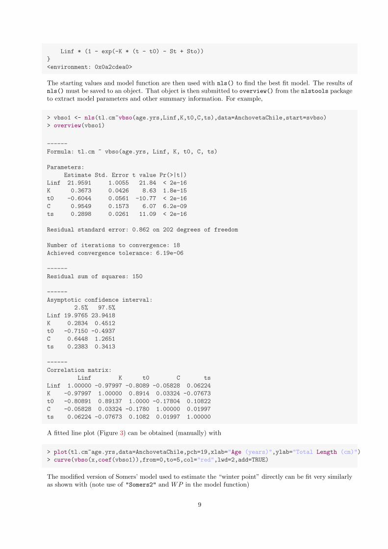
The starting values and model function are then used with nls() to find the best fit model. The results ofnls() must be saved to an object. That object is then submitted to overview() from the nlstools packageto extract model parameters and other summary information. For example,

> vbso1 <- nls(tl.cm~vbso(age.yrs,Linf,K,t0,C,ts),data=AnchovetaChile,start=svbso)

> overview(vbso1)

------

Formula: tl.cm ~ vbso(age.yrs, Linf, K, t0, C, ts)

Parameters:


Linf 21.9591 1.0055 21.84 < 2e-16

K 0.3673 0.0426 8.63 1.8e-15

t0 -0.6044 0.0561 -10.77 < 2e-16

C 0.9549 0.1573 6.07 6.2e-09

ts 0.2898 0.0261 11.09 < 2e-16




------

Residual sum of squares: 150

------

Asymptotic confidence interval:

2.5% 97.5%

Linf 19.9765 23.9418

K 0.2834 0.4512

t0 -0.7150 -0.4937

C 0.6448 1.2651

ts 0.2383 0.3413

------

Correlation matrix:

Linf K t0 C ts

Linf 1.00000 -0.97997 -0.8089 -0.05828 0.06224

K -0.97997 1.00000 0.8914 0.03324 -0.07673

t0 -0.80891 0.89137 1.0000 -0.17804 0.10822

C -0.05828 0.03324 -0.1780 1.00000 0.01997

ts 0.06224 -0.07673 0.1082 0.01997 1.00000

A fitted line plot (Figure 3) can be obtained (manually) with

> plot(tl.cm~age.yrs,data=AnchovetaChile,pch=19,xlab="Age (years)",ylab="Total Length (cm)")

> curve(vbso(x,coef(vbso1)),from=0,to=5,col="red",lwd=2,add=TRUE)

The modified version of Somers’ model used to estimate the “winter point” directly can be fit very similarlyas shown with (note use of "Somers2" and WP in the model function)

9

1 2 3 4

68

1012

1416

18

Age (years)

Tota

l Len

gth

(cm

)

Figure 3. Fitted line plot from the seasonally oscillating VBGM fit to the Chilean anchoveta data.

> svbso2 <- vbStarts(tl.cm~age.yrs,data=AnchovetaChile,type="Somers2")

> unlist(svbso2) # unlist used for display purposes only

Linf K t0 C WP

24.27855 0.02256 -0.55775 0.90000 0.90000

> ( vbso2 <- vbFuns("Somers2") )

function (t, Linf, K, t0, C, WP)

{

if (length(Linf) > 1) {

K <- Linf[2]

t0 <- Linf[3]

C <- Linf[4]

WP <- Linf[5]

Linf <- Linf[1]

}

Rt <- (C * K)/(2 * pi) * sin(2 * pi * (t - WP + 0.5))

Rto <- (C * K)/(2 * pi) * sin(2 * pi * (t0 - WP + 0.5))

Linf * (1 - exp(-K * (t - t0) - Rt + Rto))

}

<environment: 0x09ce3308>

> vbso2 <- nls(tl.cm~vbso2(age.yrs,Linf,K,t0,C,WP),data=AnchovetaChile,start=svbso2)

> overview(vbso2)

------

Formula: tl.cm ~ vbso2(age.yrs, Linf, K, t0, C, WP)

Parameters:


Linf 21.9592 1.0055 21.84 < 2e-16

K 0.3673 0.0426 8.63 1.8e-15

t0 -0.6044 0.0561 -10.77 < 2e-16

C 0.9549 0.1573 6.07 6.2e-09

WP 0.7898 0.0261 30.24 < 2e-16

10




------

Residual sum of squares: 150

------

Asymptotic confidence interval:

2.5% 97.5%

Linf 19.9765 23.9419

K 0.2834 0.4512

t0 -0.7150 -0.4937

C 0.6448 1.2651

WP 0.7383 0.8413

------

Correlation matrix:

Linf K t0 C WP

Linf 1.00000 -0.97997 -0.8089 -0.05828 0.06224

K -0.97997 1.00000 0.8914 0.03324 -0.07673

t0 -0.80891 0.89138 1.0000 -0.17804 0.10823

C -0.05828 0.03324 -0.1780 1.00000 0.01997

WP 0.06224 -0.07673 0.1082 0.01997 1.00000

11

4 Double von Bertalanffy

Vaughan and Helser (1990) introduced and Porch et al. (2002) explored the so-called “double” VBGM thatallows the fitting of one Beverton-Holt VBGM to fish less than some “critical” age (tc) and a differentBeverton-Holt VBGM to fish greater than that critical age. The model is parameterized as follows,

E[L|t] =

{L∞ ∗

(1− e−K1(t−t1)

)if t < tc

L∞ ∗(1− e−K2(t−t2)

)if t ≥ tc

(5)

where L, t, and L∞ are as defined previously, K1 and K2 are Brody growth rate coefficients for the twogroups, t1 and t2 are the ages when the average size is zero for each group, and

tc =K2t2 −K1t1K2 −K1

This model is difficult to fit because it is essentially a piecewise model where the critical point of switchingbetween the two pieces depends on parameters in the model. Thus, the model effectively contains an “if”statement. Fitting this form of model is difficult with nls() because nls() depends on derivatives of thefunction, which cannot be taken with an “if” component to the model. Fortunately, other algorithms in R– specifically, optim() – can be used to find the minimum of a function without requiring the calculation ofderivatives. Unfortunately, optim() requires a manual setup of the function to be minimized.

The process of using optim() to fit a VBGM is illustrated below, first by using optim() to fit the typicalVBGM and then showing how to use it for fitting the double VBGM. Before showing these methods, notethat hypothetical data that follows a the double VBGM with L∞=40, K1=0.412, K2=0.114, t1=0.053, t2=-8.41 parameters, resulting in , tc=3.291, was created and stored in the df data frame. A view of these datais shown below2.

> head(df)

len age

1 9.739 1

2 12.913 1

3 14.542 1

4 10.923 1

5 17.705 1

6 12.495 1

The traditional Beverton-Holt VBGM is fit to these data with nls()3

> svbs <- list(Linf=40,K=0.20,to=0)

> mdl <- len~Linf*(1-exp(-K*(age-to)))

> fit.nls <- nls(mdl,data=df,start=svbs)

> ( c.nls <- coef(fit.nls) )

Linf K to

37.3595 0.3630 -0.3064

Then, for comparative purposes, the same model is fit to the same data using optim(). To use optim(),a function must first be created that returns the predicted lengths from the model given a current set ofparameters (i.e., these parameters will change during the iterations required for fitting the model) and theobserved ages. Such a function is shown below where the first argument is a vector of parameter values4 andthe second argument is vector of the observed ages.

2The algorithm for creating these data can be seen by examining the R code script found in last section of this vignette.3Note that the starting values were found graphically with growthModelSim("vbTypical",len age,data=df).4Note that this function is hard-wired such that the first parameter must be L∞, the second must be K, and the third must

be t0.

12

> sVonB <- function(params,age) {Linf <- params[1]; K <- params[2]; to <- params[3]

Linf*(1-exp(-K*(age-to)))

}

The optim() function also requires a function that computes the residual sum-of-squares between the ob-served lengths and the predicted lengths. Such a function is shown below where the first argument is againthe vector of parameter estimates and the second and third arguments are the vectors of observed lengthsand ages, respectively. Note how this function uses the function previously constructed to find predictedlengths.

> sRSS <- function(params,len,age) { sum((len-sVonB(params,age))^2) }

Finally, optim() can be run by including the initial parameter guesses in the first argument, the RSS functionthat should be minimized as the second argument, the vectors of observed lengths and ages as the third andfourth arguments, and two arguments (hessian=TRUE and method="BFGS") that control how the optim()

routine will behave). The results should be assigned to an object as illustrated below.

> fit.o <- optim(svbs,sRSS,len=df$len,age=df$age,hessian=TRUE,method="BFGS")

The estimated parameters are extracted from the par portion of the object returned by optim() as follows

> fit.o$par

Linf K to

37.3593 0.3630 -0.3063

From this, it is evident that the parameter estimates are slightly, but imperceptibly, different between theoptim() and nls() results (Figure 4).

Using a similar process the double VBGM can fit be fit to the hypothetical data using optim(). So that thevalue of tc can be easily computed later it is useful to first construct a function to compute tc. The functionbelow performs this calculation using only a vector of parameter values as an argument5.

> tc <- function(params) {K1 <- params[2]; t1 <- params[3]; K2 <- params[4]; t2 <- params[5]

(K2*t2-K1*t1)/(K2-K1)

}

The function to constructed predicted lengths from double VBGM equation is then constructed as shownbelow. In this function, note the use of ifelse() to calculate the two “pieces” of the double VBGM.

> dVonB <- function(params,age) {Linf <- params[1]; K1 <- params[2]; t1 <- params[3]; K2 <- params[4]; t2 <- params[5]

ifelse(age<tc(params),Linf*(1-exp(-K1*(age-t1))), Linf*(1-exp(-K2*(age-t2))))

}

The function to compute the sum of squared residuals is a simple modification of the previously used function,i.e.,

5Note that this function is hard-wired such that the parameter values must be in the order of L∞, K1, K1, t1, and t2.

13

> dRSS <- function(params,len,age) { sum((len-dVonB(params,age))^2) }

Finally, optim() is used as described previously and shown below6 The final model fit is shown in (Figure4).

> dvbs <- c(37,0.36,-0.3,0.26,-3.3)

> fit.d <- optim(dvbs,dRSS,len=df$len,age=df$age,hessian=TRUE,method="BFGS")

> fit.d$par

[1] 40.1346 0.4017 0.0198 0.1114 -8.6753

> tc(fit.d$par)

[1] 3.358

6Note that there is not an automatic way to construct the starting values.

14

0 10 20 30 40

1020

3040

Age (years; jittered)

Tota

l Len

gth

(mm

)

single, nlssingle, optimdouble

Figure 4. Example of the fit of a double VBGM, (5), fit to RANDOM data.

15

5 Model of Porch et al. (2002)

WORKING ON THIS

> df$age1 <- df$age + runif(length(df$age),0.3,07)

>

>

> beta1 <- function(params,age) {> K1 <- params[4]; lambda1 <- params[5]; to <- params[3]

> K1/lambda1*(exp(-lambda1*age)-exp(-lambda1*to))

> }>

> beta2 <- function(params,age) {> K1 <- params[4]; lambda1 <- params[5]; to <- params[3]

> K2 <- params[6]; lambda2 <- params[7]; ts <- params[8]

> (K2/(4*pi^2+lambda2^2))*(exp(-lambda2*age)*(2*pi*cos(2*pi*(ts-age))-lambda2*sin(2*pi*(ts-age)))-exp(-lambda2*to)*(2*pi*cos(2*pi*(ts-to))-lambda2*sin(2*pi*(ts-to))))

> }>

> porchVB <- function(params,age) {> Linf <- params[1]; K0 <- params[2]; to <- params[3]

> Linf*(1-exp(beta1(params,age)+beta2(params,age)-K0*(age-to)))

> }>

> porchRSS <- function(params,age,len) { sum((len-porchVB(params,age))^2) }>

> pvbs <- c(43.4,0.0475,0.443,0.695,0.476,0.301,0.344,0.439)

> fit.p <- optim(pvbs,porchRSS,len=df$len,age=df$age1,hessian=TRUE,method="BFGS")

> fit.p$par

>

> pred.p <- porchVB(fit.p$par,p.ages)

> plot(len~age1,data=df,xlab="Age (years)",ylab="Total Length (mm)",pch=".")

> lines(p.ages,pred.p,col="blue",lwd=2,lty=1)

16

References

Baker, T., R. Lafferty, and T. Q. II. 1991. A general growth model for mark-recapture data. FisheriesResearch 11:257–281. 1, 5

Cubillos, L., D. Arcos, D. Bucarey, and M. Canales. 2001. Seasonal growth of small pelagic fish off Talc-ahuano, Chile (37oS, 73oW): A consequence of their reproductive strategy to seasonal upwelling? AquaticLiving Resources 14:115–124. 8

Fabens, A. 1965. Properties and fitting of the von Bertalanffy growth curve. Growth 29:265–289. 1

Francis, R. 1988. Are growth parameters estimated from tagging and age-length data comparable? CanadianJournal of Fisheries and Aquatic Sciences 45:936–942. 1, 4

Garcia-Berthou, E., G. Carmona-Catot, R. Merciai, and D. H. Ogle. 2012. A technical note on seasonalgrowth models. Reviews in Fish Biology and Fisheries 22:635–640. 6

Hoenig, N. and R. Hanumara. 1990. An empirical comparison of seasonal growth models. Fishbyte 8:32–34.6

Pauly, D. 1988. Beyond our original horizons: The tropicalization of Beverton and Holt. Reviews in FishBiology and Fisheries 8:307–334. 6

Pauly, D. and G. Gaschutz. 1979. A simple method for fitting oscillating length growth data, with a programfor pocket calculators, ices c.m. I.C.E.S. CM . Demersal Fish Comittee 1979/6:24:1–26. 6

Pauly, D., M. Soriano-Bartz, J. Moreau, and A. Jarre-Teichmann. 1992. A new model accounting for seasonalcessation of growth in fishes. Marine and Freshwater Research 43:1151–1156. 6

Pitcher, T. and P. MacDonald. 1973. Two models for seasonal growth in fishes. Journal of Applied Ecology10:599–606. 6

Porch, C. E., C. A. Wilson, and D. L. Nieland. 2002. A new growth model for red drum (Sciaenops ocellatus)that accomodates seasonal and ontogenic changes in growth rates. Fisheries Bulletin 100:149–152. 12

Somers, I. F. 1988. On a seasonally oscillating growth function. Fishbyte 6(1):8–11. 6

Vaughan, D. S. and T. E. Helser. 1990. Status of the red drum stock of the atlantic coast: stock assessmentreport for 1989. NOAA Technical Memorandum NMFS-SEFC-263, U.S. Department of Commerce. 12

Wang, Y.-G. 1998. An improved Fabens method for estimation of growth parameters in the von Bertalanffymodel with individual asymptotes. Canadian Journal of Fisheries and Aquatic Sciences 55:397–400. 3

Wang, Y.-G., M. Thomas, and I. Somers. 1995. A maximum likelihood approach for estimating growth fromtag-recapture data. Canadian Journal of Fisheries and Aquatic Sciences 52:252–259. 3

17

6 Appendix

6.1 Derivation of Fabens (1965) Increment Model

First Version

Define the length at time of marking (tm) as

Lm = L∞

(1− e−K(tm−t0)

)which is immediately rewritten as,

LmL∞

= 1− e−K(tm−t0)

LmL∞− 1 = −e−K(tm−t0)

1− LmL∞

= e−K(tm−t0)

L∞ − LmL∞

= e−K(tm−t0)

(6)

Similarly, the length at time of recapture (tr) is

Lr = L∞

(1− e−K(tr−t0)

)(7)

and define δt as “time-at-large” such that

tr = tm + δt (8)

Substitute (8) into (7) for tr and simplify,

Lr = L∞

(1− e−K(tm+δt−t0)

)Lr = L∞

(1− e−K(tm−t0)e−Kδt

)and now substitute in the last expression in (6) and simplify to get,

Lr = L∞

(1− L∞ − Lm

L∞e−Kδt

)Lr = L∞ − (L∞ − Lm) e−Kδt

Some authors will further modify this (note the addition of Lm − Lm) to get,

Lr = Lm + L∞ − Lm − (L∞ − Lm) e−Kδt

Lr = Lm + (L∞ − Lm)− (L∞ − Lm) e−Kδt

Lr = Lm + (L∞ − Lm)(1− e−Kδt

)18

Finally, other authors will present this model as a change in length,

Lr − Lm = (L∞ − Lm)(1− e−Kδt

)Second Version

Alternatively, one can start the derivation by thinking of the increment in lengths

Lr − Lm = L∞

(1− e−K(tm+δt−t0)

)− L∞

(1− e−K(tm−t0)

)Lr − Lm = L∞ − L∞e−K(tm+δt−t0) − L∞ + L∞e

−K(tm−t0)

Lr − Lm = L∞e−K(tm−t0) − L∞e−K(tm+δt−t0)

Lr − Lm = L∞e−K(tm−t0)

(1− e−Kδt

)Now, note that Lm − L∞ = −L∞e−K(tm−t0) or, more usefully, L∞ − Lm = L∞e

−K(tm−t0) which can besubstituted into the above to get

Lr − Lm = (L∞ − Lm)(1− e−Kδt

)6.2 More Algebra Related to the Fabens (1965) Model

Understanding how the Faben’s model “works” is sometimes difficult to visualize. However, some algebraon the increment model may help in this regard. Begin with,

Lr − Lm = (L∞ − Lm)(1− e−Kδt

)which is easily modified to

Lr − LmL∞ − Lm

= 1− e−Kδt

and then to

L∞ − LrL∞ − Lm

= e−Kδt (9)

which shows that Fabens model examines the relative “distances” of Lr and Lm from L∞ and models thatratio as an exponential decay model. This can be explored with hypothetical data. The predicted lengthsat six ages were computed supposing that L∞=400, K=0.5, and t0=0. All combinations of two of theselengths were then taken as a mark and recapture pair, such that the “time-at-large” was computed as thedifference in ages and the growth increment was computed as the difference in predicted lengths. The resultsare shown in Table 1 and Figure 5.

Thus, for example if the “time-at-large” (δt) is “small” (near zero) then the length-at-marking and the length-at-recapture should be approximately equal and both the LHS and the RHS of (9) will be approximatelyequal to 1. However, as the “time-at-large” increases the RHS will be smaller and Lr will be closer to L∞than Lm making the LHS also smaller.

19

Table 1. Results of several scenarious computed for hypothetical mark-recaptrue data from hypothetical vonBertalanffy data.

Scenario Ager Agem δt Lr Lm δL L∞−LrL∞−Lm

1 1.3 1.0 0.3 191.2 157.4 33.8 0.8612 2.0 1.0 1.0 252.8 157.4 95.5 0.6073 5.0 1.0 4.0 367.2 157.4 209.8 0.1354 13.5 1.0 12.5 399.5 157.4 242.1 0.0025 14.0 1.0 13.0 399.6 157.4 242.2 0.0026 2.0 1.3 0.7 252.8 191.2 61.7 0.7057 5.0 1.3 3.7 367.2 191.2 176.0 0.1578 13.5 1.3 12.2 399.5 191.2 208.3 0.0029 14.0 1.3 12.7 399.6 191.2 208.5 0.00210 5.0 2.0 3.0 367.2 252.8 114.3 0.22311 13.5 2.0 11.5 399.5 252.8 146.7 0.00312 14.0 2.0 12.0 399.6 252.8 146.8 0.00213 13.5 5.0 8.5 399.5 367.2 32.4 0.01414 14.0 5.0 9.0 399.6 367.2 32.5 0.01115 14.0 13.5 0.5 399.6 399.5 0.1 0.779

0 2 4 6 8 10 12 14

0.0

0.2

0.4

0.6

0.8

Time−at−large

'LH

S R

atio

'

1

2

3

45

6

7

89

10

11121314

15

0 2 4 6 8 10 12 14

−6

−5

−4

−3

−2

−1

0

Time−at−large

log(

'LH

S R

atio

')

12

3

45

6

7

89

10

1112

1314

15

Figure 5. Plots of the ratio (LEFT) and log ratio (RIGHT) on the LHS of (9) versus time-at-large (δt) fordata from a hypothetical von Bertalanffy growth model. The numbers correspond to the “scenario” shownin Table 1.

20

Reproducibility Information

Version Information

� Compiled Date: Fri Jun 21 2013

� Compiled Time: 6:57:06 PM

� Code Execution Time: 4 s

R Information

� R Version: R version 3.0.0 (2013-04-03)

� System: Windows, i386-w64-mingw32/i386 (32-bit)

� Base Packages: base, datasets, graphics, grDevices, methods, stats, tcltk, utils

� Other Packages: FSA 0.3.5, FSAdata 0.1.3, gdata 2.12.0.2, knitr 1.2, nlstools 0.0-14, plyr 1.8, re-shape 0.8.4, xtable 1.7-1

� Loaded-Only Packages: car 2.0-16, cluster 1.14.4, digest 0.6.3, evaluate 0.4.3, formatR 0.7, gplots 2.11.0.1,grid 3.0.0, gtools 2.7.1, Hmisc 3.10-1, lattice 0.20-15, multcomp 1.2-17, nlme 3.1-109, plotrix 3.4-7,quantreg 4.98, relax 1.3.13, sciplot 1.1-0, SparseM 0.99, stringr 0.6.2, TeachingDemos 2.9, tools 3.0.0

� Required Packages: FSA, FSAdata, nlstools and their dependencies (car, gdata, gplots, Hmisc,knitr, multcomp, nlme, plotrix, quantreg, relax, reshape, sciplot, stats, tcltk, TeachingDemos)

21

fishr vignette extra von bertalanffy - derek oglederekogle.com/.../vonbertalanffyextra.pdf · shr...

Documents