analysis, theory and design of logistic regression...
TRANSCRIPT

ANALYSIS, THEORY AND DESIGN OF LOGISTIC REGRESSION CLASSIFIERS USED
FOR VERY LARGE SCALE DATA MINING
BY
OMID ROUHANI-KALLEH
THESIS
Submitted as partial fulfillment of the requirements for the degree of Master of Science in Computer Science
in the Graduate College of the University of Illinois at Chicago, 2006.
Chicago, Illinois

This thesis is dedicated to my mother, who taught me that success is not the key to
happiness. Happiness is the key to success. If we love what we are doing, we will be
successful.
This thesis is dedicated to my father, who taught me that luck is not something that is
given to us at random and should be waited for. Luck is the sense to recognize an
opportunity and the ability to take advantage of it.
iii

ACKNOWLEDGEMENTS
I would like to thank my thesis committee – Peter C. Nelson, Bing Liu and Piotr J.
Gmytrasiewicz – for their support and assistance. With the guidance provided from them
during my research I have been able to accomplish my research goals.
I would also like to thank the Machine Learning group at Microsoft and in particular my
mentor Peter Kim for inspiring me to conduct this research with great enthusiasm and
passion.
ORK
iv
TABLE OF CONTENTS
CHAPTER ................................................................................................................ PAGE
1 INTRODUCTION..................................................................................................... 1 1.1 MOTIVATION........................................................................................................ 1 1.2 CONTRIBUTION .................................................................................................... 2 1.3 ABOUT THE ALGORITHM...................................................................................... 4
2 THEORY ................................................................................................................... 6 2.1 MACHINE LEARNING............................................................................................ 6 2.2 REGRESSION ANALYSIS ....................................................................................... 6
2.2.1 Ordinary Linear Regression ........................................................................... 7 2.2.2 General Linear Regression ............................................................................. 8 2.2.3 Logistic Regression......................................................................................... 9 2.2.4 Obtaining the Model Parameters.................................................................. 14 2.2.5 Ridge Regression .......................................................................................... 15 2.2.6 Weighted Logistic Regression....................................................................... 17
2.3 SOLVING LINEAR EQUATION SYSTEMS .............................................................. 19 2.3.1 Solving a Simple Linear Equation System .................................................... 20 2.3.2 Conjugate Gradient Method ......................................................................... 20 2.3.3 Solvers for Building Large Logistic Regression Classifiers ......................... 23 2.3.4 How to Calculate β ....................................................................................... 23 2.3.5 How to Calculate β in a Distributed Environment ....................................... 25
2.4 CLASSIFICATION AND RANKING......................................................................... 29 2.4.1 Do Classification Using Logistic Regression ............................................... 29 2.4.2 Do Ranking Using Logistic Regression ........................................................ 29 2.4.3 Different Accuracy Measures ....................................................................... 30 2.4.4 Top N Accuracy............................................................................................. 30 2.4.5 Accuracy of the System ................................................................................. 31 2.4.6 Obtaining top N Accuracy ............................................................................ 32 2.4.7 Avoid Over Fitting the Classifier.................................................................. 37
2.5 DOING ON-THE-FLY PREDICTION ...................................................................... 39 2.5.1 Algorithm Overview...................................................................................... 39 2.5.2 Algorithm Analysis........................................................................................ 43
3 EXPERIMENTS ..................................................................................................... 45 3.1 OVERVIEW OF OUR NETWORK........................................................................... 45 3.2 OVERVIEW OF EXPERIMENTS ............................................................................. 45 3.3 DATA SETS ........................................................................................................ 46 3.4 COMPARING LOGISTIC REGRESSION WITH NAÏVE BAYES .................................. 47 3.5 RIDGE COEFFICIENT TUNING ............................................................................. 54
3.5.1 Improvement of Top 10 Accuracy ................................................................. 58 3.6 RESIDUAL TUNING............................................................................................. 59
4 FUTURE RESEARCH........................................................................................... 61
v

TABLE OF CONTENTS (continued)
CHAPTER................................................................................................................ PAGE
5 CONCLUSIONS ..................................................................................................... 62
REFERENCES................................................................................................................ 64
APPENDIX...................................................................................................................... 66
VITA................................................................................................................................. 87
vi

LIST OF TABLES
TABLE ...................................................................................................................... PAGE
I. PROPERTIES OF THE 10 DIFFERENT DATA SETS WE HAVE USED. ...... 47
II. ACCURACY IN TERMS OF TOP 1 ACCURACY............................................ 53
III. ACCURACY IN TERMS OF TOP 10 ACCURACY.......................................... 53
IV. OPTIMAL RIDGE VALUES............................................................................... 57
vii

LIST OF FIGURES
FIGURE .................................................................................................................... PAGE 1. Schematic overview of the system.......................................................................... 3
2. Ordinary Linear Regression.................................................................................... 8
3. Generalized Linear Regression ............................................................................... 9
4. The logit function.................................................................................................. 11
5. The odds function ................................................................................................. 13
6. The conjugate gradient method............................................................................. 21
7. Algorithm for Obtaining β (IRLS)........................................................................ 24
8. Server pseudo code for distributing which β each client should calculate ........... 28
9. Algorithm to calculate the top N accuracy, single process................................... 33
10. Algorithm to calculate the β’s and calculate the Class and Score matrices.......... 35
11. Code to merge two Score and Class matrices together......................................... 36
12. Algorithm for Fast On-the-Fly Prediction ............................................................ 42
13. The Accuracy in terms of top 1 accuracy ............................................................. 50
14. Accuracy in terms of top 10 accuracy................................................................... 51
15. Correlation between ridge coefficient and the accuracy, top 1 accuracy ............. 56
16. Correlation between ridge coefficient and the accuracy, top 10 accuracy ........... 56
17. Improvement due to parameter tuning.................................................................. 58
18. Accuracy for different residuals............................................................................ 60
viii

LIST OF ABBREVIATIONS
LR Logistic Regression
NB Naïve Bayesian
CG Conjugate Gradient
IRLS Iteratively Reweighted Least-Squares
ix

SUMMARY
This thesis proposes a distributed algorithm to efficiently build a very large scale logistic
regression classifier. Previous work in the field has shown success building logistic
regression classifiers that are large in terms of number of attributes, but due to the
computational complexity of the methods available it has been infeasible to scale up the
classifiers to handle very large number of classes (on the order of 100,000 classes or
more).
We will propose an algorithm that given a large number of client machines can efficiently
build a logistic regression classifier. The proposed algorithm will deal with issues such as
over fitting the classifier, failing client machines, load balancing and avoidance of
redundant read and write operations to our database.
We will also present an algorithm showing how logistic regression can be used to build a
classical large scale search engine that can do fast on-the-fly prediction.
Finally we will use large public data sets to analyze how well logistic regression performs
in comparison to the naïve Bayesian classifier. We will see what kind of parameter tuning
is necessary and what properties of the data sets affect the accuracy of the classifier. We
will also see how well the logistic regression classifier performs when we use different
measures of accuracy and how different parameter tuning can optimize the classifier for
the different measures.
x

1 Introduction
1.1 Motivation
In recent days, more and more papers have been reporting success in using logistic
regression in machine learning and data mining applications in fields such as text
classification [11] and a variety of pharmaceutical applications. Methods have also been
developed for extending logistic regression to efficiently be able to do classification on
large data sets with many prediction variables [1].
However, so far no approaches have been publicly suggested to scale up a logistic
regression classifier to be able to deal with very large datasets in terms of (i) number of
attributes, (ii) number of classes and (iii) number of data points
Even the largest data sets that have been used to build logistic regression classifiers have
been small in either one or two of the above mentioned size measures. Often, the number
of classes has been relatively small (usually on the order of tens or hundreds of classes).
This is often due to the fact that many practical applications often have a very limited
number of classes. For example we want to classify an article to one of a small number of
categories, or we might want to classify some symptoms to one of a small number of
diseases.
However, in some real life applications such as the ranking of classes we need to be able
to scale up the classifier to deal with a very large number of classes. For instance, we
might want to build a system that can rank a very large number of documents, given a
large set of features. In such an application it is not enough to be able to build a classifier
that can classify or rank tens or hundreds of documents, but we want be able to scale the
classifier to ten thousands or hundred thousands of documents.
1

2
1.2 Contribution
Our work builds on a recent proposed technique for using logistic regression as a data
mining tool [1]. The proposed technique scales well for data sets with a large number of
attributes and large data sets, but has the drawback of not being able to scale well for data
sets with a large set of classes.
We propose an algorithm that will run on a distributed system that will be able to build a
logistic regression classifier that not only scales well in the number of attributes and size
of the data size, but also in the number of classes.
We will also propose an algorithm that allows us to do fast on-the-fly prediction of new
previously unseen data points. This is a basic requirement for us to be able to use this
system in a search engine that should be able to deal with a large work load predicting
user queries in a fast pace.
The algorithm will run on one server machine and an arbitrary number of client
machines. In our experiments we have had 68 Pentium 4 (2.4 – 2.8 GHz) Linux client
machines building the classifier. The job of the server is to fairly distribute the jobs that
have to be computed among the client machines. The clients will have access to a
database where they will be able to store the results of their calculations.
Figure 1 shows a schematic overview of the system.
3
Figure 1 Schematic overview of the system. The clients can access a data base for data storage (and retrieval) and sending commands to a server. The server can not contact the clients and hence does not know if a client, at any particular moment in time, is dead or alive.
The algorithm has the following properties:
• It is failure tolerant. Hence it can nicely deal with clients that crash or are taken
down abruptly. Any, or even all, clients can crash at the same time, and the loss of
computed data will be limited to the very last jobs that the failing clients were
working with.
• It has load balancing. So we ensure that the work amount that is given to each
client is in direct proportion to the performance of that client machine.
• The algorithm ensures that the number of read and write operations that the client
machines are doing to the database is kept to a minimum by using caching of
computed data and using heuristics to avoid too many clients to be working on
redundant jobs.
• The algorithm avoids over fitting the classifier by calculating the accuracy of the
classifier after each iteration of the algorithm. Hence, the accuracy will not be
dependent on arbitrarily chosen termination criteria, but the training will go on as

4
long as the accuracy increases. This can be done with a very small number of
overhead read and write operations to the database.
• The algorithm can efficiently build a logistic regression classifier when the data
set is large in terms of the number of classes, the number of attributes and the
number of data points.
1.3 About the Algorithm
To be able to build such a large classifier we need an algorithm that can scale up well.
First of all, it will not be possible to build the entire classifier with just one machine. The
weight matrix in our logistic regression system will have as many rows as we have
number of classes, and each row will take on the order of 1 minute to calculate when the
size of the problem is around 100,000 attributes and 1’000’000 data points. So assuming
we want to build a classifier with 100,000 classes or maybe even more, this will take
around 100,000 minutes, or around 69.4 days. For this we need to have an algorithm that
scales up well. In the ideal case, we would achieve a linear speed up in the number of
processors we have. Our algorithm will achieve close to a linear speed up.
However, in practice it is reasonable that we take into account events such as client
failures, load balancing and other network failures. Since even if a large machine stack
might be able to finish the work relatively fast, we want to avoid situations where one
source of failure (such that a client machine goes down or that the network goes down)
leads to a failure of our algorithm. Also, we want be able to implement this algorithm on
a distributed system where all of the clients are unreliable. Our algorithm is failure

5
tolerant, so any or even all clients can go down of the same time (or even the server can
be temporary disconnected from the network), and the algorithm will still be able to
continue from right before the failure (or very close to that point).
The algorithm assumes the clients to be non-malicious, so even if we can handle cases
where client machines are terminated at any step of the execution, we at all time assume
no processes are malicious. This basically means that the clients are not “lying” to the
server by sending untruthful commands to the server (for example, claiming that they
have finished a job they have not finished). Hence, the algorithm will be able to run on
any distributed corporate network where the clients are “nice”, but the algorithm will not
(without extensions) be able to run on arbitrary machines on the internet where a
malicious “hacker” might purposely try to mislead the server with false messages.
2 Theory
2.1 Machine Learning
Machine learning is a subfield of Artificial Intelligence and deals with the development
of techniques which allows computers to “learn” from previously seen datasets. Machine
learning overlaps extensively with mathematical statistics, but differs in that it deals with
the computational complexities of the algorithms.
Machine learning itself can be divided into many subfields, whereas the field we will
work with is the one of supervised learning where we will start with a data set with
labeled data points. Each data point is a vector
[ ]nxxxx ,...,, 21=
and each data point has a label
{ }myyyy ,...,, 21∈ .
Given a set of data points and the corresponding labels we want be able to train a
computer program to classify new (so far unseen) data points by assigning a correct class
label to each data point. The ratio of correctly classified data points is called the accuracy
of the system.
2.2 Regression Analysis
Regression analysis is a field of mathematical statistic that is well explored and has been
used for many years. Given a set of observations, one can use regression analysis to find
a model that best fits the observation data.
6

7
2.2.1 Ordinary Linear Regression
The most common form of regression models is the ordinary linear regression which is
able to fit a straight line through a set of data points. It is assumed that the data point’s
values are coming from a normally distributed random variable with a mean that can be
written as a linear function of the predictors and with a variance that is unknown but
constant.
We can write this equation as
εβα ++= xy *
where α is a constant, sometimes also denoted as b0, β is a vector of the same size as our
input variable x and where the error term
),0( 2σε Ν∈ .
Figure 2 shows a response with mean
xy *35.045.2 +−=
which follows a normal distribution with constant variance 1.
8
Figure 2 Ordinary Linear Regression Ordinary Linear Regression for y = -2.45 + 0.35 * x. The error term has mean 0 and a constant variance.
2.2.2 General Linear Regression
The general form of regression, called generalized linear regression, assumes that the data
points are coming from a distribution that has a mean that comes from a monotonic
nonlinear transformation of a linear function of the predictors. If we can call this
transformation g, the equation can be written as
εβα ++= )*( xgy
where α is a constant, sometimes also denoted as b0, β is a vector of the same size as our
input variable x and where the error term is ε.
9
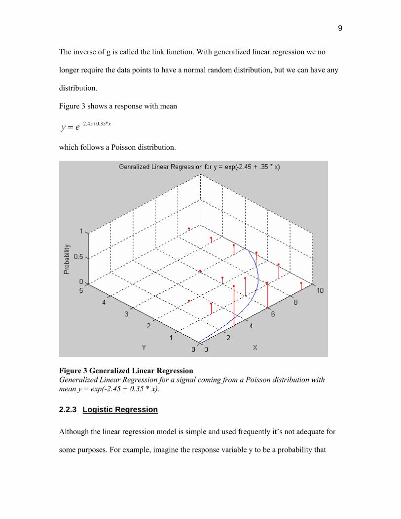
The inverse of g is called the link function. With generalized linear regression we no
longer require the data points to have a normal random distribution, but we can have any
distribution.
Figure 3 shows a response with mean
xey *35.045.2 +−=
which follows a Poisson distribution.
Figure 3 Generalized Linear Regression Generalized Linear Regression for a signal coming from a Poisson distribution with mean y = exp(-2.45 + 0.35 * x).
2.2.3 Logistic Regression
Although the linear regression model is simple and used frequently it’s not adequate for
some purposes. For example, imagine the response variable y to be a probability that

10
takes on values between 0 and 1. A linear model has no bounds on what values the
response variable can take, and hence y can take on arbitrary large or small values.
However, it is desirable to bound the response to values between 0 and 1. For this we
would need something more powerful than linear regression.
Another problem with the linear regression model is the assumption that the response y
has a constant variance. This can not be the case if y follows for example a binomial
distribution (y ~ Bin(p,n)). If y also is normalized so that it takes values between 0 and 1,
hence y = Bin(p,n)/n, then the variance would then be Var(y) = p*(1-p), which takes on
values between 0 and 0.25. To then make an assumption that y would have a constant
variance is not feasible.
In situations like this, when our response variable follows a binomial distribution, we
need to use general linear regression. A special case of general linear regression is
logistic regression, which assumes that the response variable follows the logit-function
shown in Figure 4.

11
Figure 4 The logit function Note that it’s only defined for values between 0 and 1. The logit function goes from minus infinity to plus infinity. The logit function has the nice property that logit(p) = -logit(1-p) and its inverse is defined for values from minus infinity to plus infinity, and it only takes on values between 0 and 1.
However, to get a better understanding for what the logit-function is we will now
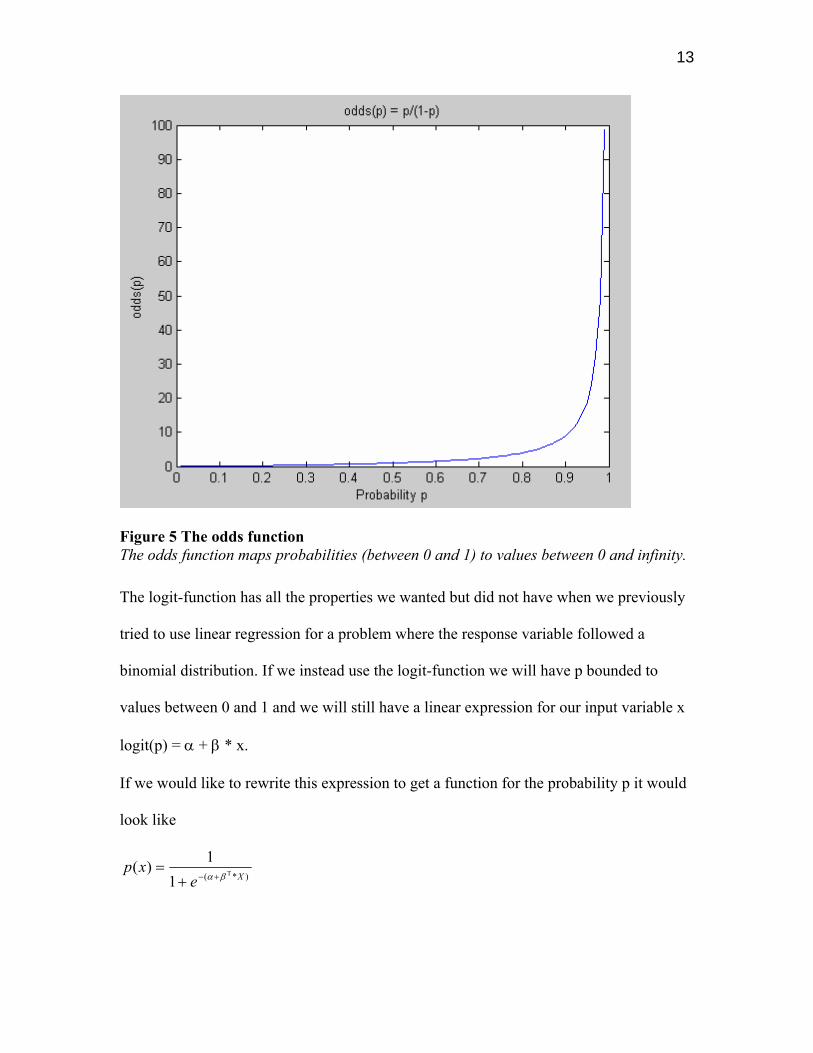
introduce the notation of odds. The odds of an event that occurs with probability P is
defined as
odds = P / (1-P).
Figure 5 shows how the odds-function looks like. As we can see, the odds for an event is
not bounded and goes from 0 to infinity when the probability for that event goes from 0
to 1.
However, it’s not always very intuitive to think about odds. Even worse, odds are quite
unappealing to work with due to its asymmetry. When we work with probability we have

12
that if the probability for yes is p, then the probability for no is 1-p. However, for odds,
there exists no such nice relationship.
To take an example: If a Boolean variable is true with probability 0.9 and false with
probability 0.1, we have that the odds for the variable to be true is 0.9/0.1 = 9 while the
odds for being false is 0.1/0.9 = 1/9 = 0.1111... . This is a quite unappealing relationship.
However, if we take the logarithm of the odds, when we would have log(9) for true and
log(1/9) = -log(9) for false.
Hence, we have a very nice symmetry for log(odds(p)). This function is called the logit-
function.
logit(p) = log(odds(p)) = log(p/(1-p))
As we can see, it is true in general that logit(1-p)=-logit(p).
logit(1-p) = log((1-p)/p) = - log(p/(1-p)) = -logit(p)
13
Figure 5 The odds function The odds function maps probabilities (between 0 and 1) to values between 0 and infinity.
The logit-function has all the properties we wanted but did not have when we previously
tried to use linear regression for a problem where the response variable followed a
binomial distribution. If we instead use the logit-function we will have p bounded to
values between 0 and 1 and we will still have a linear expression for our input variable x
logit(p) = α + β * x.
If we would like to rewrite this expression to get a function for the probability p it would
look like
)*( T
11)(
Xexp
βα+−+=

14
2.2.4 Obtaining the Model Parameters
In practice, one usually simplifies notation somewhat by only having one parameter β
instead of both α and β.
If our original problem is formulated such as
εβα ++= *xy
We rewrite this as
εβα += Txy ],[*],1[
If we now call β’ = [α β] T and x’ = [1 x] then we can formulate the exact same problem
but with only “one” model parameter β’
εβ +′′= *xy .
Note that this is nothing but a change of notation. We still have two parameters to
determine, but we have simplified our notation so that we now only need to estimate β’.
From now on, we will denote β’ as β and x’ as x and our problem statement will hence be
to obtain the model parameter β when
εβ += *xy
If we have made n observations with responses yi and predictors xi we can define
TnyyyY ],...,,[ 21=
TnxxxX ],...,,[ 21= .
The system we want to solve to find the parameter β is then written as
β*XY = .
The minimum square error solution to this system is found as follows
β*XY =

15
β*** XXYX TT =
YXXX TT **)*( 1−=β .
We just need to evaluate the expression (XT * X)-1 * X T * Y and we have found the β
that minimizes the sum of squares residuals. However, in practice there might be
computational difficulties with evaluating this expression, as we will see further on.
2.2.5 Ridge Regression
As we have seen we can obtain β by simply evaluating
YXXX TT **)*( 1−=β .
However, if some prediction variables are (almost) linearly dependent, then XT * X is
(almost) singular and hence he variance of β is very large. So to avoid having XT * X
singular we add a small constant value to the diagonal of the matrix
YXIXX TT **)**( 1−+= λβ
where I = unity matrix, and λ = small constant.
By doing this we avoid the numerical problems we will get when trying to invert an
(almost) singular matrix. But we are paying a price for doing this. By doing this we have
biased the prediction and hence we are solving the solution to a slightly different
problem. As long as the error due to the bias is smaller than the error we would have got
from having a (nearly) singular XT * X we will end up getting a smaller mean square
error and hence ridge regression is desirable.
We can also see ridge regression as a minimization problem where we try to find a β
according to
16
( )∑ −−i
Tii Xy 2*
,minarg βαβα
stsj
j ≤∑ 2.. β .
Which we (through Lagrange multiplier) can rewrite to an unconstraint minimization
problem
( ) ∑∑ +−−j
ji
Tii Xy 22 **
,minarg βλβαβα
where λ is inversely proportional to s.
This can be compared to the classic regression where we are minimizing
( )∑ −−i
Tii Xy 2*
,minarg βαβα
.
Now the problem is just to find a good λ (or s) so that the variance gets small, but at the
same time we should make sure the bias error doesn’t get to big either. To find a good λ
(or s) we can use heuristics, graphics or cross validation. However, this can be
computationally expensive, so in practice one might prefer to just choose a small constant
λ and then normalize the input data so that
∑ =i
ix 0
and
∑ =i
i
nx
1 .
Or in other words, we make sure x is centered and normalized.
Ridge regression has the advantage of preferring smaller coefficient values for β and
hence we end up with a less complex model. This is desirable, due too Occam’s razor

17
which says that it is preferable to pick the simpler model out of two models that are
equally good but where one is simpler than the other, since the simpler model is more
likely to be correct and also hold for new unseen data.
Another way to get an intuition for why we prefer small coefficient values is in the case
when we have correlated attributes. Imagine two attributes that are strongly correlated
and when either one of them takes the value 1, the other one does the same with high
likelihood and vice verse. It would now be possible that the coefficients for these two
attributes to take identical extremely large values but with different signs since they both
“cancel out” each other. This is of course undesirable in the situations when the attributes
take different values and X * β takes on ridiculously large values.
Ridge regression has proved itself to be superior to many alternative methods when it has
been used to avoid numerical difficulties when solving linear equation systems for
building logistic regression classifiers ([1], [2], [13]).
Ridge regression was first used in the context of least square regression in [15] and later
on used in the context of logistic regression in [16].
2.2.6 Weighted Logistic Regression
As we have seen we need to evaluate this expression in classic logistic regression
YXXX TT **)*( 1−=β
This expression came from the linear equation system
β*XY = .
Indirectly we assumed that all observations where equally important and hence had the
same weight, since we tried to minimize the sum of squared residuals.

18
However, when we do weighted logistic regression we will weight the importance of our
observations so that different observations have different weights associated to them. We
will have a weight matrix W that is a diagonal matrix with the weight of observation i at
location Wii.
Now, instead of evaluating
YXXX TT **)*( 1−=β
we will evaluate
UWXXWX TT ***)**( 1−=β
where
)1(*
*
iiii
ii
iiTii
WW
yXU
μμ
μβ
−=
−+=
and μi is our estimate for p, which we previously saw could be written as
βμ
*11
TiXi
e−+= .
The weights Wii are nothing but the standard deviation of our own prediction. In general,
if
),(~ npBinX
then
)1(**)( ppnXVar −=
and since we have a Bernoulli trial we have n = 1 so the variance becomes
)1(* iiiiW μμ −= .
The term yi - μi is our prediction error and the variance Wii “scales” it so that a low
variance will have a larger impact on U than a high variance data point. Or in other

19
words, the importance of correctly classifying data points with a low variance increases
while the importance of correctly classifying data points with a high variance decreases.
2.3 Solving Linear Equation Systems
We have now seen the theory behind the equation that we now need to solve. With
notation as before we now want to solve
UWXIXWX TT ***)***( 1−+= λβ .
However, so far we have not discussed the computational difficulties with doing this.
One of the major differences between classical statistics and machine learning is that the
later one deals with the computational difficulties one is facing when one is trying to
solve the equations obtained from the field of classical statistics.
When one needs to evaluate an expression such as the one we have for β, it is very
common to write down the problem as a linear equation system that needs to be solved,
to avoid having to calculate the inverse of a large matrix.
Hence, the problem can be rewritten as
bA =β*
where
IXWXA T *** λ+=
UWXb T **= .
Let us now take a closer look at the problem we are facing.
What we want to achieve is to build a classifier that will classify very large data sets. Our
input data is X and (indirectly) U. To get an idea of what size our matrices have, imagine
our application having 100,000 classes and 100,000 attributes, also imagine us having in

20
average 10 training data points per class. The size of the A matrix would then be 100,000
x 100,000 and the size of the b vector would be 100,000 x 1. The X matrix would be of
size 1’000’000 x 100,000. Luckily for us, our data will be sparse, and hence only a small
fraction of the elements will have non-zero values. Using this knowledge, we can choose
an equation solver that is efficient given this assumption.
2.3.1 Solving a Simple Linear Equation System
In general when one needs to solve a linear equation system such as
bA =β*
one needs to choose a solver method appropriate to the properties of the problem. This
basically means that one needs to investigate what properties are satisfied for A and from
that choose one of the many available solver methods that are available. If one needs an
iterative solver, which does not give an exact solution but is computationally efficient and
in many case the only practical alternative, [3] offers an extensive list of solvers that can
be used.
2.3.2 Conjugate Gradient Method
For our application we are going to use the conjugate gradient method, which is a very
efficient method for solving linear equation systems when A is a symmetric positive
definite matrix, since we only need to store a limited number of vectors in memory.
When we solve a linear system with iterative CG we will use the fact that the solution to
the problem A * β = b, for symmetric positive definite matrices A, is identical to the
solution for the minimization problem

21
ββββ
****5.0minarg TT bA − .
The complete algorithm for solving bA =β* using the CG algorithm is found in Figure
6.
Conjugate Gradient Algorithm:
Input: A, b, maximum number of iterations imax and a starting value x. Output: x such as A x = b.
new
Tnew rr
rdxAbr
i
δδδ
==
=−=
=
0
*0
while newδ is large enough and maxii <
1*
**
*
+=+=
=
=
=−=+=
=
=
iidrd
rr
qrrdxx
qd
dAq
old
new
Tnew
newold
Tnew
βδδβ
δ
δδαα
δα
end
Figure 6 The conjugate gradient method The conjugate gradient method can efficiently solve the equation system A * β = b, for symmetric positive definite sparse matrices A.
With perfect arithmetic, we will be able to find the correct solution x in the CG algorithm
above in m steps, if A is of size m. However, since we will solve the system A * β = b
iteratively, and our A and b will change after each iteration, we don’t iterate the CG

22
algorithm until we have an exact solution for β. We stop when β is “close enough” to the
correct solution and then we recalculate A and b, using the recently calculated β value,
and once again run the CG algorithm to obtain an even better β value. So although the
CG algorithm requires m steps to find the exact solution, we will terminate the algorithm
in advance and hence get a significant speed up.
How fast we get to a solution that is good depends on the eigenvalues of the matrix A.
We earlier stated that m iterations are required to find the exact solution, but to be more
precise the number of iterations required is also bounded by the number of distinct
eigenvalues of matrix A. However, in most practical situations with large matrices we
will just iterate until the residual is small enough. Usually we will get a solution that is
reasonable good within 20-40 iterations.
Note that one might choose many different termination criteria for when we want to stop
the CG algorithm. For example:
• Termination when we have iterated too many times.
• Termination when residual is small enough
ε<− 2* bXA .
• Termination when the relative difference of the deviance is small enough
εβ
ββ<
−−
2
1
)()()(
i
ii
devdevdev .
The deviance for our logistic regression system is
( ) ( )( )∑ −−+−=i
iiii yydev μμβ 1log)1(log*2)( 22
where as previously

23
βμ
*11
TiXi
e−+= .
For an extensive investigation of how different termination criteria are affecting the
resulting classifier accuracy, see [9].
For the reader interested in more details about the conjugate gradient method and
possible extensions to it, the authors would like to recommend [3], [7] and [8].
2.3.3 Solvers for Building Large Logistic Regression Classifiers
Many papers have been investigating how one can build large scale logistic classifiers
with different linear equations solvers ([1], [4], [5], [6]). We will be using the conjugate
gradient method for this task. This has previously been reported to be a successful
method for building large scale logistic classifiers in terms of nr of attributes and in nr of
data points ([1]). However, due to the fact that the high computational complexity of
calculating β it is infeasible to build very large logistic regression classifiers if we don’t
have an algorithm for building the classifier in a distributed environment using the power
of a large number of machines.
The main contribution of this research will be to develop an efficient algorithm for
building a very large scale logistic regression classifier using a distributed system.
2.3.4 How to Calculate β
We have now gone through all theory we need to be able to build a large scale logistic
regression classifier. To obtain β we will now be using the iteratively reweighted least-
squares method, also known as the IRLS method in Figure 10.
A complete algorithm for getting β is shown in Figure 7.

24
Algorithm for Obtaining β (IRLS) Input: Matrix X (rows corresponding to data points and columns to prediction attributes), vector y (rows corresponding to data points, takes values of 0 or 1) and ridge regression constant λ. Output: Model parameter β. Notation: Xi means row i of matrix X. vi means element i of vector v.
0=β while termination criteria is not met
UWXbIXWXA
WyXU
We
u
T
Tii
iiii
iiii
Xi i
*****
)(*
)1(*1
1*
=
+=
−+=
−=+
= −
λ
μβ
μμ
β
Solve β from bA =β* using CG algorithm. end
Figure 7 Algorithm for Obtaining β (IRLS) The Iteratively Reweighted Least-Squares method algorithm.
Note that this will give us β for one class only. We need to run this algorithm once for
each class that we have so that we have one β for each class. If we for example have
100,000 classes, the algorithm would need to run 100,000 times with different yi values
each time. To run this code with a data set with around one million data points that have
in the order of 100,000 attributes could take in the order of 1 minute to finish, so to be
able to scale up our classifier we need an algorithm that can efficiently run this piece of
code on distributed client machines.

25
2.3.5 How to Calculate β in a Distributed Environment
We have already discussed how we can calculate β using the IRLS algorithm together
with a conjugate gradient solver. So in the scenario where we have n classes and we need
to create n different β’s we just need to run the IRLS algorithm n times.
For small values of n this is reasonable to do on one single machine, however, when n
approaches higher number, close to 10’000 or above, it is desirable to have multiple
machines running the same code in parallel calculating all β’s in parallel.
If we would have n classes and p processors one naïve algorithm could be to divide the n
classes in p equally sized sets and let each processor finish its part and store all β’s in a
common database. However, an algorithm such as this suffers from several draw backs.
First of all, we don’t have any load balancing. One processor might finish its work faster
than the other processes and hence we would end being idle while there still is more work
that it could be doing. Second, the algorithm would not be failure tolerant. Any of the
machines might go down or stop responding, and we would end up waiting for the
completion of jobs that will never be completed. The only way to detect such a failure
would be for clients to regularly check each others status (or having a separate server that
does this) to make sure that no other client has been taken down. This is not a realistic
approach to take.
Another approach one could take would be that each client informs all other clients (with
a network broadcast message) as soon as it has started calculating β and when it is done
calculating β it sends another message letting everyone know it has finished the
calculation. After this is done, the client would need to get a confirmation from all the
other clients that it alone has calculated β and that it can proceed by storing the value in

26
the database to avoid having multiple processes trying to write to the same file on a
possible file server at once with possible data corruption as a result. However, a protocol
such as this would not be feasible in an environment where clients might fail since one
single process failure would halt all other processes due to that it can not send the
acknowledgement that is necessary for the other processes before they can write β to the
data base. We would prefer a system where the clients concentrate on the number
crunching necessary to calculate β, and not to run complex message passing algorithms
talking to each other discussing who shall do what.
So our solution to how to fairly distribute the job is to have a server/client solution where
the server is a coordinator telling the clients what to do. The client will send commands
to the server asking for what job should be done, and the server who has an overall
picture of what has been calculated and what needs to be calculated will respond telling
the client what needs to be done next.
We will also associate one lock for each β. The lock is given by the server to the client
when the client has finished calculating β and want store the result of the calculation to
database. Note that multiple processes can be working on calculating the same β at the
same time, but at most one process can have the lock for β at any given time, and hence
at most one process will try to store β to the database at any given time. This does not
only avoid the problem of ending up with a corrupt file in case two processes try to write
to the same file at the same time, but it also ensures that the load on the database is kept
to a minimum. We will do exactly 1 write operation per β to the database. Since β has a
fix size this allows us to calculate in advance the exact load we will cause to the database

27
due to the β write operations. This property is also highly desirable if we choose to
implement our database as a distributed storage system.
Each lock is also associated with a timer. If a lock is given to a process and the process
fails before the lock is handed back to the server, the server will tell the other clients that
the lock has not been released and that the client who has the lock needs to be terminated
before the lock is released. Figure 8 shows pseudo code for the server.

28
Server pseudo code for distributing which β each client should calculate
When client wants to calculate a β If there exists β that is not stored in database then
Return any β that has not been stored to database yet. We should use some heuristic here to minimize the likelihood of two processes calculating the same β. For example, give the β that was given away longest time ago.
else Tell the client no β needs to be calculated.
end When client has calculated β If all β has been stored to database then
Tell the client that β has already been calculated and stored to database. elseif lock for β has not been handed out then
Give lock for β to client, allowing him to write β to database. elseif lock for β has already been handed out then
if no lock that we have handed out has timed out then Ask the client to sleep for a while, and send the same command again later.
else From now on, ignore any messages sent from the process who locked β. Ask the client to terminate the execution of the process that has the lock for β and then report this back to us. When client reports back to us confirming that it has terminated the process that has the lock, the lock for β is released.
end end When client has saved β to database Keep track of that β has been stored to the database.
Figure 8 Server pseudo code for distributing which β each client should calculate The algorithm described how the server decides which β each client should start calculating.
When the clients have finished creating all β we are done with one step of the iteration.
To avoid over fitting our classifier we now want to know the over all accuracy of the
classifier before we start with the next iteration. Before we discuss how we can get the
accuracy for the entire system, we will discuss how we can do classification using

29
logistic regression and we will also introduce the notation of top N accuracy, which we
will be using to determine how accurate our classifier is.
2.4 Classification and Ranking
2.4.1 Do Classification Using Logistic Regression
The way we will do classification with our system when we have all β values is to create
a matrix that we call the “weight matrix” (denoted W).
Say we have a data point x and we want to know which of the n classes it should belong
to.
We have previously seen that the probability that data point x belongs to the class
corresponding to β is
xexp
*11)(
β−+= .
Hence, the larger value we have for β * x, the stronger is our belief that the data point x
belongs to the class corresponding to β. So to do classification, we only need to see
which β gives the highest value and chose that class as our best guess.
( )xxClassify ii *maxarg)( β= .
2.4.2 Do Ranking Using Logistic Regression
To do ranking, we do basically the same thing as for classification
xiScore i *)( β= .
Hence, the score for class i will be βi * x, and we rank the classes so that the class with
the highest score is ranked highest.

30
2.4.3 Different Accuracy Measures
There exist several different approaches with different pros and cons when it comes to
determining the accuracy of a classifier. One of the most popular approaches is the k-fold
validation, where we divide the data set in k subsets and we build the classifier with k-1
of the subsets and validate the accuracy with the k:th subset, and then we repeat this k
times with one of the k subsets chosen as validation data each time.
The advantage of this approach is that we even with small data sizes can use a large
portion of our data to actually build the classifier. However, we need to build the
classifier k times, which is time consuming if the training phase of the algorithm takes
long time to run.
For our algorithm we need to take a different approach. The training phase is what really
takes time and we can not afford to build a classifier k times just to get the system
accuracy. Our algorithm is intended for very large data sets where we don’t have a
shortage of data. So we will simple divide our dataset into two subsets. One that is used
for training and one that is used for validation.
2.4.4 Top N Accuracy
The accuracy measure we will have for our classifier is something we will call “top N
accuracy”. When we are doing classification with very large amount of classes, for
example 100,000 classes, it is very hard to get a good accuracy even if we have a good
classifier. If we have a data point x, it can be hard to correctly classify it when there are
so many classes to choose from, and hence, reporting the accuracy of the system with the
classical notation of accuracy as ratio of correctly classified classes can be misleading.

31
For this reason we introduce the notation “top N accuracy” which means that we consider
a data point to have been correctly classified if our classifier was able to rank the data
point among the top N classes in its ranking.
This notation of accuracy makes sense in many real life applications. Assume for
example someone is doing a search for a particular document/article/file and we have an
application that will be listing 10 search results. We can say that as long as the correct file
is somewhere among these 10 results, then the classifier has succeeded in the ranking,
while it would have failed if none of these 10 documents were the document the user
where looking for.
One can extend this notation if desired to a weighted top N accuracy notation so that we
score how well the document is ranked among these top N documents. Basically, we
want the classifier to get a higher accuracy if the correct class is ranked at top of the
search result, and lower accuracy if the document is located at the bottom of the search
result.
However, in this paper we are assuming a non-weighted “top N accuracy” notation, and
hence we either say that the classifier classified data point x correctly, or incorrectly,
without giving score to “how well” it classified the data point.
Note that when N=1 our “top N accuracy” is the same thing as the classical notation of
accuracy for a classifier.
2.4.5 Accuracy of the System
Since we are going to use this algorithm to build very large classifiers, we are interested
in the top N accuracy for the system. However, it can be hard to know what N we shall

32
choose. For this reason we want our algorithm to be able to record the top N accuracy for
all N in a fix interval, for example N = 1, 2, …, 100.
As a user of the system we can then easily see what top N accuracy we have obtained,
without having to revalidate the system with large amount of validation data. Instead, we
just need to run the algorithm once and when it has terminated we can see all top N
accuracies for all N we have chosen.
2.4.6 Obtaining top N Accuracy
We have already seen how we can do classification and ranking with our system.
We are now interested in finding a way to calculate the top N accuracy for a large amount
of N = 1, 2, … with our algorithm.
Before we discuss how we have solved this in the distributed scenario, let us take a look
on how we can do this in the single processor scenario.
Imagine that we have already calculated all β’s and now want the top N accuracy for N =
1, 2, …, m. Figure 9 shows how we will get the desired top N accuracy.
The algorithm basically stores the top N ranks for each validation data point in two
matrices Score and Class. After sorting these two matrices row-wise we have that Classi,j
tells us which class we have ranked at position j for data point i. Scorei,j is the
corresponding score. The higher score Scorei,j, the more certain the classifier is that data
point i corresponds to the class Classi,j.
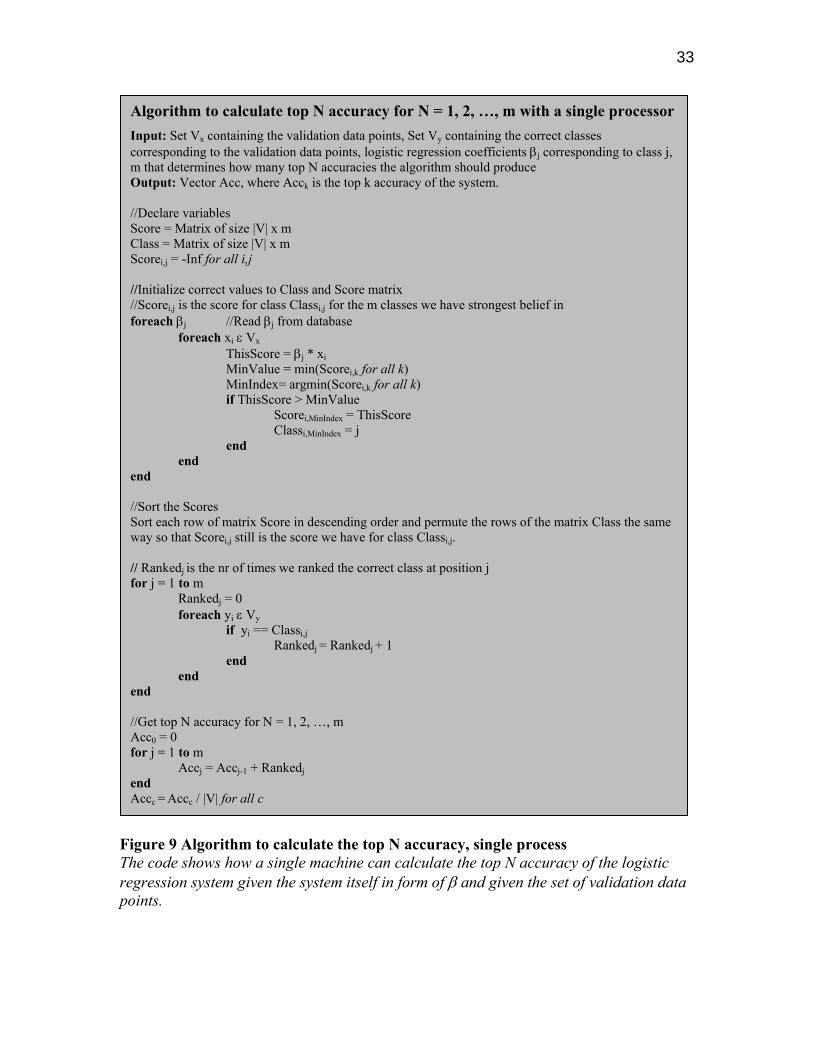
33
Algorithm to calculate top N accuracy for N = 1, 2, …, m with a single processor Input: Set Vx containing the validation data points, Set Vy containing the correct classes corresponding to the validation data points, logistic regression coefficients βj corresponding to class j, m that determines how many top N accuracies the algorithm should produce Output: Vector Acc, where Acck is the top k accuracy of the system. //Declare variables Score = Matrix of size |V| x m Class = Matrix of size |V| x m Scorei,j = -Inf for all i,j //Initialize correct values to Class and Score matrix //Scorei,j is the score for class Classi,j for the m classes we have strongest belief in foreach βj //Read βj from database foreach xi ε Vx
ThisScore = βj * xi MinValue = min(Scorei,k for all k)
MinIndex= argmin(Scorei,k for all k) if ThisScore > MinValue Scorei,MinIndex = ThisScore Classi,MinIndex = j end end end //Sort the Scores Sort each row of matrix Score in descending order and permute the rows of the matrix Class the same way so that Scorei,j still is the score we have for class Classi,j. // Rankedj is the nr of times we ranked the correct class at position j for j = 1 to m Rankedj = 0 foreach yi ε Vy if yi == Classi,j
Rankedj = Rankedj + 1 end
end end //Get top N accuracy for N = 1, 2, …, m Acc0 = 0 for j = 1 to m
Accj = Accj-1 + Rankedjend Accc = Accc / |V| for all c
Figure 9 Algorithm to calculate the top N accuracy, single process The code shows how a single machine can calculate the top N accuracy of the logistic regression system given the system itself in form of β and given the set of validation data points.

34
Note that the algorithm uses each βi only once, which is very desirable, since each βi can
be quite large and needs to be read from disc.
In the case where we have a distributed system with the client machines separated from
the database where βi is stored each read of βi is equivalent to accessing the network and
downloading βi from the database. The number of elements for each βi is the same as the
number of attributes our classifier has, and we have one βi for each class, so assuming we
have a problem of size 100,000 attributes and 100,000 classes and each element of βi is
for example 4 bytes, that would put a 40 gigabyte load on the server database. This is
both time consuming and puts a heavy load on the database.
We will see how we can avoid this load by joining the two algorithms for creating βi and
for calculating the top N accuracy into one algorithm, where we directly after creating βi
start calculating the Score and Class matrices. This has the advantage that when the client
has just created βi it will have it stored in main memory, and since we only need the value
once we can start calculating the Score and Class matrices before all other βi‘s are
calculated.

35
Pseudo code for client to calculate the β’s and calculate the Class and Score matrices for the β’s we have calculated Scorei,j = -Inf for all i,j while there are β’s left to calculate
Ask the server for a β to calculate (see Figure [8]). Calculate β (see Figure [7]). if we can obtain lock for β from server (see Figure [8]).
Store β to database (see Figure [8]). Update the Score and Class matrices using β (see Figure [9]).
end end Store the partially calculated Score and Class matrix to server
Figure 10 Algorithm to calculate the β’s and calculate the Class and Score matrices The code shows how a single machine can calculate the Class and Score matrices that are necessary for our algorithm to be able to determine the accuracy of the system when it is built, without having to read all the β’s from the database.
With Figure 10 we will not only calculate all the β’s as we did previously, but each client
will also have the Score and the Class matrix partially calculated. We have done this
without adding any extra messages sent by the client and without adding any extra work
load on the database. Just as before we only write β to the server once and we don’t need
to read it back from the database later on since we have already used the β to calculate
the Score and the Class matrices.
What we need to do is to merge all the partially calculated Class and Score matrices into
one single Class and Score matrix, that can be used to calculate the score for the entire
system. A partially calculated Score and Class matrix contains information about which
N classes are highest ranked for each validation data point, among the classes that were
used to build the specific Score and Class matrix. When two clients merge their matrices
together (according to Figure 11), the resulting matrix will contain which N classes are

36
highest ranked for each validation data point, among the classes that were used to create
the two initial matrices.
Pseudo code for how to merge two Score and Class matrices together Input: Score matrices Score1 and Score2 and Class matrices Class1 and Class2, m is the number of columns the matrices have Output: Score matrix Scorenew and Class matrix Classnew i=1 Foreach row of Scorenew
Create row i of Scorenew by taking the highest m values from row i of matrices Score1 and Score2.Create row i of Classnew by taking the Class1 and Class2 values that corresponds to the highest score values we previously picked. i = i + 1.
end
Figure 11 Code to merge two Score and Class matrices together The code shows how a single machine can merge two Score and Class matrices into just one Score and Class matrix. When our system is done building the entire classifier we will have stored all β’s in the database and each client machine will have one Score and Class Matrix. It would be inefficient to load all β’s back into memory to obtain the accuracy of the classifier. Instead we can pass around and merge the Score and Class matrices until only one single Score and Class matrix remains, which will contain the top N accuracy of our system.
As Figure 11 shows it’s very easy to merge two partially calculated Class and Score
matrices into one new Class and Score matrix. What we need to do now is to let the
clients merge the matrices until we end up with only one Class matrix and one Score
matrix. Figure 9 shows how we calculate the top N accuracy from a Class and Score
matrix.
Each node will have created one partially computed Class and Score matrix, so a system
with n nodes will have n partially computed matrices. If a node would fail or time out so

37
we can not access the matrices it has stored, the server will give the jobs that it previously
has given to the failed client to the remaining processors.
For a single machine it is O(n) to merge all these partial results into the final result, one
single Class and Score matrix.
However, our system will use the fact that we have n processes that each can take 2
partial results and merge them into one new partial result. Process p1 will merge result r1
with result r2 (call the new result r1,2), p2 will merge r3 with r4 to r3,4, p3 will merge r5 with
r6 to r5,6 etc. In a fix amount of time have reduced the number of partially results ri from n
to n/2. In total, we will in time O(log(n)) convert all partially computed matrices into one
final result r1,2,…,n. This will correspond to the final Score and Class matrix we will use to
calculate the accuracy of the entire classifier.
2.4.7 Avoid Over Fitting the Classifier
Now when all the partial matrices have been calculated and we have the accuracy of the
system, it is up to the server to determine if it should continue iterating or if we should
terminate the algorithm. Recall that the purpose of calculating the top N accuracy for the
system after each iteration is so that we can do small iteration steps and after each
iteration step see what the current accuracy of the system is. It can otherwise be hard to
choose good termination criteria for a classifier of this size. Now we don’t have to decide
termination criteria in advance, we just go on and iterate until we don’t see any
improvement of the accuracy. Doing this we will avoid terminating the training phase too
early or over fitting the classifier since we will after each iteration determine if the
classifier’s accuracy is improving or not. As long as we save the β’s for the best classifier
we have calculated we can even roll back and say that the β’s we had after the i:th

38
iteration gave the highest accuracy and should hence be used as our final classifier. All
β’s calculated after the optimal β’s are considered over fitted and can be thrown away.

39
2.5 Doing On-the-Fly Prediction
2.5.1 Algorithm Overview
We have presented an algorithm that scales up well and that can be used to do fast
classification on large data sets with an accuracy that outperforms the naïve Bayesian
classifier. However, this comes to the price of greater complexity both in terms of time to
build the classifier and in the resources needed to be able to build it. The weight matrix
W has memory complexity O(a * c) where a is the number of attributes and c is the
number of classes. Assuming 100,000 attributes and 100,000 classes and 4 bytes per
element in the matrix, the matrix will be in the order of 40 gigabytes. This is way too
large to be able to be used for classification on one single machine. This has been the
main drawback of logistic regression when using large data sets. When we built the
classifier we obtained the accuracy of the entire system after each iteration step without
having to store the entire W matrix in main memory at any point in time. Instead we used
the fact that we only need one row of the W matrix in the main memory at any point in
time to build the Class and Score matrices, that later could be merged together so we end
up with only one Class and Score matrix that has the total accuracy of the entire system.
However, to do this we used batched data points for validation. When we want to do on-
the-fly prediction of data points one at a time we must use an other approach. Assume
that we want that our logistic regression system to be used to do fast on-the-fly prediction
on sparse input data points with a good top N accuracy. This is identical to the scenario of
having a search engine that takes a few keywords as input and that should output a list of

40
N documents that are related to the keywords. The input vector is sparse (since only a
few keywords are used) and N is very small in comparison to the total number of classes
(a very small fraction of the total number of documents are listed in the search result).
We will when we build the classifier see exactly what accuracy it has, but when we want
to do fast on-the-fly prediction of single data points (search queries) we can’t do this
using a single server machine. The size of the weight matrix W is too large for one single
machine to be able to do fast prediction. When we design a search engine, or any other
system that needs to do fast prediction, it’s desirable to store all memory that will
frequently be used directly in the main memory to get a high performance on the overall
system. To achieve this with our system we need to use our distributed system also for
the prediction. We will have one machine serving as the central server and n other servers
serving as distributed servers, each holding one small part of the W matrix (essentially it
stores a subset of all the β’s, as many as the main memory allows). When we want to do
prediction on a previously unseen data point x we send this to the central server who
forwards this to all the distributed servers. Assuming that x is a sparse vector with
Boolean values, this would just require a few bytes to be sent from the central server to
each other server machine. These servers will respond with the Class and Score matrices
corresponding to the classes they have in memory, and the central server will merge all
the returned Class and Score matrices using the algorithm presented in Figure 11. After
merging all the Class and Score matrices the central server will know which N classes are
the most likely classes to correspond to data point x. The Class and Score matrices will in
the case of prediction of one single data point be of size 1 x N, hence for realistic values
for N this will be just a few bytes of data that has to be sent from each distributed server

41
to the central server. Note that as long as the input data has at most a fix number of
attributes set (hence, it’s a sparse vector) and the values of the input data is either 0 or 1
the classification per server will be done with O( c ) addition operations. We don’t need
to actually implement a matrix-vector multiplication since we only add the weight
elements corresponding to the indexes of input data x that are set to 1, and then return the
N largest sums. We don’t even need to do any scalar multiplications. Hence, with this
system we will be able to do on-the-fly prediction even for very large matrices W, as long
as we have several servers that can run in parallel.
With all this said, the authors want to emphasize that it will not be possible to build a
good search engine with the standards we have today by only using a logistic regression
classifier, but with this algorithm one would be able to build a high performance logistic
regression classifier as a component in a larger classifier system that can do classification
in real time. A increasingly number of papers have lately been published suggesting that
the accuracy of the logistic regression classifier is good enough to compete with other
more traditional machine learning techniques, and with the algorithm proposed in this
paper the performance will also be acceptable to be used in large real life systems.

42
Algorithm for Fast On-the-Fly Prediction Example illustrates system being used as a search engine. The input will be the K keywords used in the user query and the values of the Class vector will correspond to the indexes of the N documents presented as search result. We will be using 1 central server and D distributed servers, each storing Ti rows of the weight matrix, i = 1, …, D. Input: Sparse input vector x, where xi = 1 if keyword i has been used in user query, otherwise xi = 0. Output: Vector ClassFinal, where ClassFinali is the index of the i:th document in the search result.
• Central server receives x. • Central server forwards x to each distributed servers. (O(K) bytes transmitted). • Each distributed server receives x and calculate the Score for each class it is
responsible for. This is done by adding the weights corresponding to the attributes in x that are set to 1. No matrix-vector multiplication is needed since our input attributes are assumed to be binary. (O(K * Ti) addition operations).
• The distributed server stores the indexes of the N highest Score values in a vector called Class. This is equivalent to pick out the N smallest values from a list of Ti values. (O(min(N * Ti,Ti*log(Ti))), since N often is much smaller than Ti (and since N is independent of the size and dimension of the data set), we have O(N * Ti)).
• The distributed server sends the Score and Class vector to the central server. (O(N) bytes transmitted).
• The central server merges all the Score and Class vectors received into ScoreFinal and ClassFinal. This is equivalent to pick out the N smallest values from a list of N*D values. (O(min(N2 * D, N * D * log(N * D)))).
• The central server returns the search result list in which the i:th document corresponds to the document with index ClassFinali.
Total Time Complexity: Bytes transmitted between central server and the distributed servers: O(K + N) bytes to each distributed server. Operations per distributed server i: O((K + N) * Ti) Operations for central server: O(min(N2 * D, N * D * log(N * D)))
Figure 12 Algorithm for Fast On-the-Fly Prediction The code shows how a system of distributed computers can be used to perform very fast real time classification (on-the-fly classification) using a very large logistic regression system that does not fit in memory on one single machine. In this example, we call the input ‘keywords’ and the output ‘documents’ to relate to our research focus. However, the algorithm is general and works for any system that has sparse input data and where the system shall return the N most likely classes out of D classes, where N << D.

43
2.5.2 Algorithm Analysis
Figure 12 shows the algorithm for fast on-the-fly prediction and is both scalable and can
work even with very large datasets. It however requires that we have several servers
dedicated for the task of doing prediction, but since each classification takes a very short
time to do, one will be able to do a large number of predictions in parallel.
Note that we can fix the maximum number of keywords allowed per query (K) and also
fix how many documents are listed in the search result page (N), so both K and N are
small fixed numbers. Ti depends on the memory available in each distributed server. The
more memory we have, the more rows from the weight matrix can we store in main
memory and hence Ti will be larger. D depends on the size of the weight matrix, which
depends linearly on the number of keywords and documents we have.
To get a notion of the size of the system we are talking about we will look on an example
system with 100,000 documents and 100,000 keywords. Assuming 32 bits floating point
precision the weight matrix would require 40 GB storage. Using distributed servers with
2 GB memory each we would need 20 distributed servers, each storing 5’000 rows of the
weight matrix. Hence, D=20 and Ti=5000, for all i.
Note that the work load on the central server only increases linearly with the number of
distributed servers that we have, and the work load of the distributed servers only
increases with the number of rows from the matrix that it stores.
Also note that all operations we are doing are basic additions, comparisons and
assignments. We don’t need to use any matrix-vector multiplications, which allows for an
efficient implementation of the system.

44

3 Experiments
3.1 Overview of Our Network
Our algorithm will be run on unreliable machines in a network separated from the server
computer. We will be using 68 Pentium 4 (2.4-2.8 GHz) Linux machines to build and test
the classifiers. The machines that will be used are all lab machines in the university’s
computer lab and can hang or be shut down at any time. The machines have network
access directly to each other, but are protected with firewalls from external machines.
The machines will be able to communicate through HTTP to the server informing the
server of what the client have accomplished and to ask the server for what needs to be
done next. Since HTTP is a one-request-one-response type of protocol the server can only
send information to the clients as responses to the HTTP requests. Our “database” is the
university’s file system so anything that according to the algorithm is stored in “the
database” will be stored as a file on our file system. Note however that the algorithm has
completely abstracted the notation of a “database”. In practice it is up to the implementer
if we want to use a central database, a central file system or even a distributed storage
solution. Recall that the algorithm guaranteed that at most one client machine will write
to the same file at any point in time, which is a very nice property if we one day would
choose to use a distributed storage medium for our data base.
3.2 Overview of Experiments
We have investigated how the data set size and how the choice of the ridge parameter
affects the accuracy of the ranking system. Our experiments will show that a ranking
system that performs optimally w.r.t. top 1 accuracy does not necessarily perform
45

46
optimally w.r.t. top 10 accuracy. We have investigated how the choice of parameters
should differ when the priority is not to achieve a high top 1 accuracy, but rather a high
top 10 accuracy.
We also have compared how a logistic regression classifier performs w.r.t. a naïve
Bayesian classifier. We will show that although the logistic regression classifier overall
outperforms the naïve Bayesian classifier, there is a strong correlation between the data
set size and the performance improvement.
Our choice to compare the logistic regression classifier to the naïve Bayesian classifier is
because the naïve Bayesian classifier has been investigated for a long period of time and
proven to be both simple and yet give a good accuracy. The naïve Bayesian classifier
requires no parameter tuning as oppose to other classifiers such as Support Vector
Machines, and hence the accuracy obtained will not depend on the authors’ choice of
parameters.
We believe that an analysis based on the naïve Bayesian classifier will give the fairest
and most unbiased report of the actual accuracy of our system.
3.3 Data Sets
The data sets we have been using are public data sets available for download from
internet. The data comes from the Internet Movie Database, IMDb.com.
Each row of the data corresponds to a movie title or series on television. The attributes
and classes correspond to actors/actresses. A data point corresponds to all the
actors/actresses in a particular movie, except one person. The classifier should predict
who the missing actor/actress is.
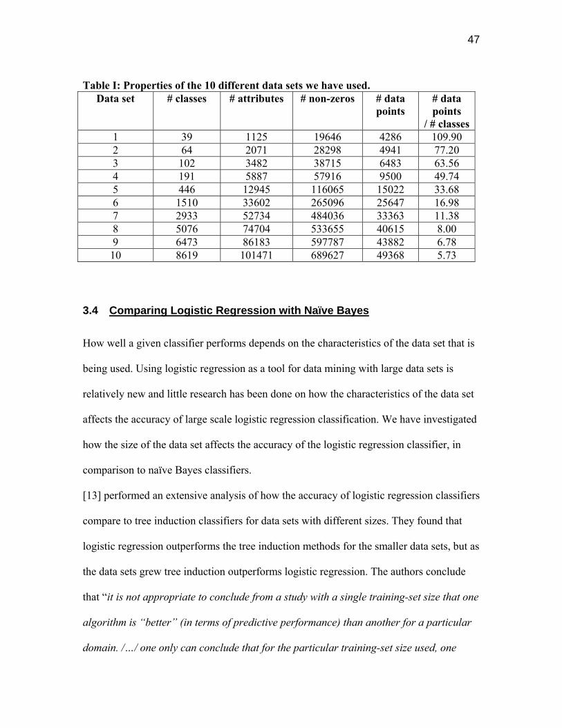
47
Table I: Properties of the 10 different data sets we have used.
Data set # classes # attributes # non-zeros # data points
# data points
/ # classes1 39 1125 19646 4286 109.90 2 64 2071 28298 4941 77.20 3 102 3482 38715 6483 63.56 4 191 5887 57916 9500 49.74 5 446 12945 116065 15022 33.68 6 1510 33602 265096 25647 16.98 7 2933 52734 484036 33363 11.38 8 5076 74704 533655 40615 8.00 9 6473 86183 597787 43882 6.78 10 8619 101471 689627 49368 5.73
3.4 Comparing Logistic Regression with Naïve Bayes
How well a given classifier performs depends on the characteristics of the data set that is
being used. Using logistic regression as a tool for data mining with large data sets is
relatively new and little research has been done on how the characteristics of the data set
affects the accuracy of large scale logistic regression classification. We have investigated
how the size of the data set affects the accuracy of the logistic regression classifier, in
comparison to naïve Bayes classifiers.
[13] performed an extensive analysis of how the accuracy of logistic regression classifiers
compare to tree induction classifiers for data sets with different sizes. They found that
logistic regression outperforms the tree induction methods for the smaller data sets, but as
the data sets grew tree induction outperforms logistic regression. The authors conclude
that “it is not appropriate to conclude from a study with a single training-set size that one
algorithm is “better” (in terms of predictive performance) than another for a particular
domain. /…/ one only can conclude that for the particular training-set size used, one

48
algorithm performs better than another”. Basically, the authors find that given a data set
for a particular domain, the accuracy obtained by the classifiers depends on the size of the
data set. In particular, the authors write “we can see a clear criterion for when each
algorithm is preferable: C4 for high-separability data and logistic regression for low-
separability data”.
[17] compares logistic regression to several adaptive non-linear learning methods and
concludes that none of the methods could outperform logistic regression. The authors
however write “we suspect that adaptive nonlinear methods are most useful in problems
with high signal-to-noise ratio”.
The graph in Figure 13 shows the accuracy of the naïve Bayesian classifier and the
logistic regression classifier as a function of the average number of data points per class,
using the data sets in Table I. The logistic regression classifier consistently performed
slightly better than the naïve Bayesian classifier. This result is consistent with the theory
as well ([18]). This holds throughout our data sets.
If we look on the data sets with smallest number of data points per class we see that the
naïve Bayesian classifier performs significantly worse than the logistic regression
classifier, which supports the theory that logistic regression’s big advantage occurs for
data sets with few data points per class, as also suggested by [13]. When we have a larger
amount of data points per class we reach the asymptotic classification accuracy and
logistic regression performs consistently slightly better than the naïve Bayesian classifier.
Note that if the Gaussian assumptions hold and the size of the data set reaches infinity,
then the accuracy of the Bayesian classifier and the logistic regression classifier will
(theoretically) be identical. However, in practice the assumption rarely does hold,

49
resulting in a slight decrease of accuracy due to the faulty assumption. The price we have
to pay in order to use a logistic regression classifier is in terms of a more complex
classifier.
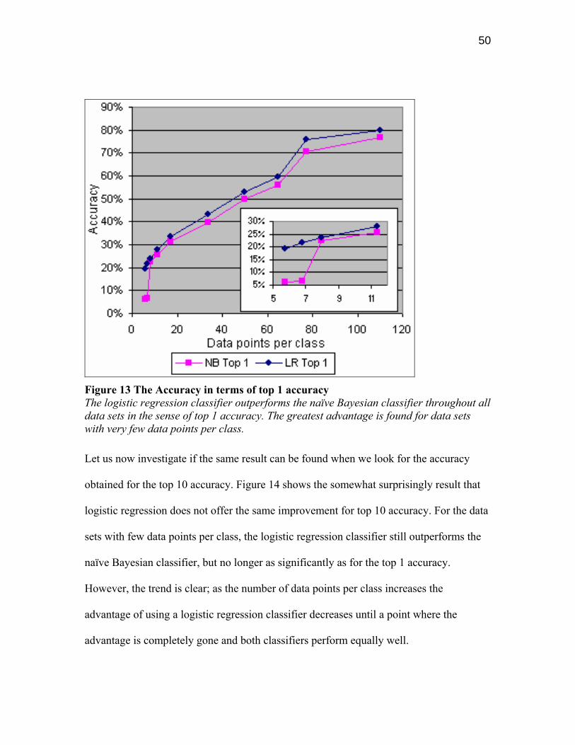
50
Figure 13 The Accuracy in terms of top 1 accuracy The logistic regression classifier outperforms the naïve Bayesian classifier throughout all data sets in the sense of top 1 accuracy. The greatest advantage is found for data sets with very few data points per class.
Let us now investigate if the same result can be found when we look for the accuracy
obtained for the top 10 accuracy. Figure 14 shows the somewhat surprisingly result that
logistic regression does not offer the same improvement for top 10 accuracy. For the data
sets with few data points per class, the logistic regression classifier still outperforms the
naïve Bayesian classifier, but no longer as significantly as for the top 1 accuracy.
However, the trend is clear; as the number of data points per class increases the
advantage of using a logistic regression classifier decreases until a point where the
advantage is completely gone and both classifiers perform equally well.

51
Figure 14 Accuracy in terms of top 10 accuracyWhen we define accuracy in terms of top 10 accuracy the logistic regression classifier no longer outperforms the naïve Bayesian classifier. The logistic regression classifier only obtains a higher accuracy for the data sets with very few data points per class.
Although the naïve Bayesian as often as the logistic regression classifier could predict the
correct class among the top 10 most likely classes, it more often predicted an incorrect
class at the top position of the list of most likely classes. We find this result interesting
and we have not seen it reported in previous literature.
To do multi-class classification with M classes we build M separate binary classifiers,
each learning to classify one class (usually with one-class-against-the-rest classification).
To pick out the N most likely classes given a data point we let all classifiers score the
data point and the N classifiers with the highest scores correspond to the classes we have
most belief in. The underlying assumption here is that when we train each separate binary
classifier to get a high top 1 accuracy this will also give us a high top N accuracy when
we combine all the M binary classifiers to one multi-class classifier. Our results clearly
52
contradict this. The logistic regression classifier outperformed the naïve Bayesian
classifier in the sense of top 1 accuracy. However, if the classifiers had been used in an
application where we ask the classifiers to not only return one class, but multiple classes,
they both perform equally well (neglecting the data sets with few data points per class
when the asymptotic accuracies have not yet been reached and the logistic regression
classifier still performs slightly better).
The detailed results from our experiments are shown in Table II and III.

53
The accuracy of the naïve Bayesian and the logistic regression classifier for the 10 different data sets. The improvement column shows how many percent more data points the LR classifier could classify correctly compared to the NB classifier. The accuracy is in term of the top 1 accuracy. Table II Accuracy in terms of top 1 accuracy
Top 1 accuracy Dataset Logistic
Regression Naïve Bayesian Improvement
Dataset 1 19,46% 6,32% 207,91%Dataset 2 21,76% 6,56% 231,71%Dataset 3 23,71% 22,42% 5,75%Dataset 4 27,95% 25,55% 9,39%Dataset 5 33,54% 31,21% 7,47%Dataset 6 43,06% 39,73% 8,38%Dataset 7 52,80% 49,98% 5,64%Dataset 8 59,44% 56,23% 5,71%Dataset 9 75,79% 70,68% 7,23%Dataset 10 79,74% 76,66% 4,02%
As table II, but for the top 10 accuracy. Table III Accuracy in terms of top 10 accuracy
Top 10 accuracy Dataset Logistic
Regression Naïve Bayesian Improvement
Dataset 1 37,20% 30,15% 23,38%Dataset 2 40,99% 37,98% 7,93%Dataset 3 44,53% 43,22% 3,03%Dataset 4 51,81% 52,00% -0,37%Dataset 5 60,57% 60,61% -0,07%Dataset 6 70,81% 70,81% 0,00%Dataset 7 80,84% 81,26% -0,52%Dataset 8 85,25% 85,99% -0,87%Dataset 9 92,87% 92,34% 0,57%Dataset 10 96,27% 97,01% -0,77%
54
3.5 Ridge Coefficient Tuning
Although the theory suggests that the ridge parameter should be tuned whenever ridge
regression is used, many researchers ([1], [13], [14]) have previously chosen to use a
fixed ridge value during their experiments, suggesting that the accuracy of the classifier is
not significantly dependent of the choice of parameter. [1] presented ridge logistic
regression as a parameter free classifier.
Such a property would be desirable since it would mean that logistic regression should be
considered a parameter free classifier that could be implemented in software packages
that do not require any parameter tuning and hence are easy to use. However, our
experiments show this property does not necessarily hold, but is instead dependent on the
size of the data set.
We have analyzed some previous publications that did not use any parameter tuning to
see if there might have been an intentional decision with a purpose to neglect the
parameter tuning. [13] for example only experiments with one fix value for the ridge
coefficient and finds that “the technique was less successful” than the other classifiers in
their comparison, although they also find that “ridge logistic regression was occasionally
effective for small samples”1 since it achieved high accuracies for some of their small
data sets. The authors continue, “we used one particular method of choosing the ridge
parameter λ; perhaps some other choice would have worked better, so our results should
not be considered a blanket dismissal of the idea of ridge logistic regression”. The
authors do not mention what ridge value was actually used for their experiments.
1 This statement is consistent with our results that will show that logistic regression performs best for data sets with very few data points per class.

55
In another recent paper [1] present the ridge logistic regression as a parameter free
classifier and writes “unlike most LR implementations, we provide no parameter tuning
instructions, because none are needed”. The authors use 10 as the default parameter for
all their data sets. The authors however write “common wisdom says that the ridge
regularization parameter should be tuned per-dataset using cross validation. However,
we have not yet been tempted to adjust this parameter for any dataset”.
For our data sets we have analyzed how different choices for the ridge coefficient will
affect the accuracy of the classifier. Figures 15 and 16 show the graphs for the top 1 and
top 10 accuracy, respectively, for one randomly chosen data set.
Each classifier for the varying ridge values was built multiple times using different
termination criteria. The most accurate classifier was selected. Thus our experiments are
invariant to the fact that a different number of iterations may be necessary to optimize the
classifier accuracy for different ridge coefficient values.
As shown in Figures 15 and 16, there is a clear correlation between the choice of the
ridge value and the accuracy of the classifier. Figures 15 and 16 show there is a single
ridge value (or perhaps a small interval) corresponding to an optimal classifier for a given
data set. Table IV shows the optimal ridge values for each of the data sets. The table
shows that a larger ridge value is necessary for the classifier to perform optimally in
terms of top 10 accuracy.

56
Figure 15 Correlation between ridge coefficient and the accuracy, top 1 accuracyThere is a significant correlation between the (top 1) accuracy of the classifier and the constraint put on the weight coefficients through the ridge value. Graph is for data set 6.
Figure 16 Correlation between ridge coefficient and the accuracy, top 10 accuracy The optimal top 10 accuracy is obtained with a higher ridge value than what was necessary for the top 1 accuracy. A higher ridge value forces the weight coefficients to take on lower values resulting in a more robust classifier. Graph is for data set 6.

57
The table shows how many percent more data points the LR classifier could classify correctly compared to the NB classifier. We note the following: (i) The LR classifier is robust and performs well for the data sets with very few data points where the NB classifier breaks down. (ii) To obtain a more robust classifier that can perform well in terms of top 10 accuracy we need to choose a larger ridge value than what we use to obtain a high top 1 accuracy. (iii) The LR classifier outperforms the NB classifier in the traditional measure of accuracy (top 1), but not for the top 10 measure of accuracy that is important in applications when ranking is used.Table IV Optimal ridge values
Top 1 accuracy Top 10 accuracy Data set
LR accuracy improve
ment over NB
Optimal ridge value
LR accuracy improve
ment over NB
Optimal ridge value
1 207,91% 2 23,38% 4 (+2) 2 231,71% 2 7,93% 6 (+4) 3 5,75% 4 3,03% 6 (+2) 4 9,39% 2 -0,37% 6 (+4) 5 7,47% 2 -0,07% 7 (+5) 6 8,38% 2 0,00% 3 (+1) 7 5,64% 1 -0,52% 2 (+1) 8 5,71% 4 -0,87% 4 (+0) 9 7,23% 1 0,57% 2 (+1) 10 4,02% 2 -0,77% 2 (+0)
Although not depicted in Table IV, a closer analysis of both our own data sets and the
data sets used by other researchers suggests that accuracy is dependent on the selection of
a ridge value. For data sets with a very small number of data points per class the classifier
is much more sensitive to parameter tuning compared to data sets with a larger number of
data points per class. Our different data sets had an average between 5.7 and 109.9 data
points per class. When we consider only reasonable ridge values in the range 1 to 15 to
determine how much gain in accuracy could be obtained by tuning the parameter, we
found a clear pattern where data sets with fewer data points per class obtained a higher
accuracy gain using parameter tuning, as Figure 7 shows. This result is not inconsistent

58
with the assertion of [1] that parameter tuning is unnecessary, as their data sets had a very
large number of data points per class.
Figure 17 Improvement due to parameter tuningParameter tuning has a significant impact on the accuracy for data sets with very many classes where each class corresponds to only a few data points. The graph shows how many percent more data points were correctly classified when parameter tuning was used.
Although it might be time consuming and practically difficult, to find an optimal ridge
value for a given data set, it appears worthwhile to at least empirically try a small number
of different ridge values to interpolate where the maximum of the accuracy curve is to
select a final ridge value that gives a close-to-optimal classifier.
3.5.1 Improvement of Top 10 Accuracy
During our experiments we looked for patterns in how different choices of ridge values
impacted the accuracy of the classifiers both in terms of top 1 accuracy and in terms of
top 10 accuracy. Our main purpose was to see if an optimal ridge value in terms of the
top 1 accuracy also could be used to build an optimal classifier in terms of the top 10
accuracy. We found a clear pattern in all our data sets showing that the ridge value that
gave an optimal top 10 accuracy had to be greater than the ridge value that performed
best in the sense of top 1 accuracy.

59
One might have expected that a ridge value that gives a good top 1 accuracy also gives a
good top 10 accuracy, but our experiments show otherwise. This is because a larger ridge
value forces the coefficients in the weight matrix to take on smaller values, leading to a
model that becomes more stable in the sense that the absence or presence of an attribute
does not affect the ranking score as heavily as it would if the weight matrix consisted of
large values. An abnormal value for an attribute does not lead to a significant decrease or
increase of the score, and hence the correct class is more likely to stay among the top
rank even if the data point contains abnormalities in its attribute values.
3.6 Residual Tuning
When we solve the linear equation system A * x = b we do so by using the conjugate
gradient method. We must choose termination criteria, preferably both in terms of
number of iterations and in the maximum allowed residual. We found that the choice of
parameters are crucial for the accuracy of the classifier. To find the exact solution using
the conjugate gradient method one needs to iterate m times, where m is the number of
distinct eigenvalues of the matrix. However, in our case m will be in the order of the size
of the data set. For even modestly large data sizes this becomes infeasible. Instead, we
iterate until we have reached a predefined number of iterations or until the residual is
small enough. The trade off between doing many iterations or just doing a few is solely a
trade off between training time to build the classifier and the final accuracy obtained
since more iterations mean we get a better approximation of the vector x compared to the
true value of x.
To investigate how the choice of the residual parameter changed the systems overall
accuracy we built the classifier several time using the same data set but with different

60
residual parameters. As expected the accuracy increases with lower residual parameters,
but when we go below 0.001 we no longer see any significant improvements. This holds
throughout our experiments with different data sets even though the data sets have
significantly different sizes and hence the conjugate gradient method had to find solutions
to problems with a variety of different sizes. Other authors have previously made similar
conclusions. For example [1] has also independently selected 0.001 as a good threshold
value to be used for all the data sets in the experiments conducted, although their data
sets have different characteristics than ours.
Figure 18 Accuracy for different residuals Choosing a suitable residual value is a tradeoff between low training time vs. high accuracy. We see that a residual smaller than 0,001 does not offer any improvement in accuracy, and is hence unnecessary.

4 Future Research
As our results shows, logistic regression performed as best when our measure of accuracy
was top 1 accuracy. For the data sets with many data points per class the performance for
the top 10 accuracy was comparable to the naïve Bayesian classifier.
An interesting question is whether this is a data set property or a classifier property? Does
it hold in general that certain classes of classifiers are better for top 1 accuracy, compared
to their performance for top N accuracy? These are important questions for researchers
working with data mining tools where the top N accuracy is a more appropriate
measurement of the true performance of the tool used than the traditional measure of
accuracy (which is often the case in applications where a system ranks or give score to a
large set of classes).
In our experiments we have chosen to only investigate the top 1 accuracy and the top 10
accuracy of the logistic regression classifier since 10 is a reasonable number in many
practical applications (show 10 search results, 10 best matching addresses, 10 book
suggestions etc.), but one might ask if the performance is likely to fall even more for
larger N? One possible theory could be that classifiers with larger degree of freedom in
general obtains higher top 1 accuracy, but lower accuracy in the sense of top N accuracy
due to the higher degree of freedom. However, to make general conclusions regarding
this further research needs to be performed in this field.
61

5 Conclusions
In this thesis we have proposed several algorithms to be able to scale up the logistic
regression classifier and use it in the field of large scale online search technology. We
have also done a comprehensive analysis of the logistic regression classifier and its usage
in the field of machine learning and data mining. The combination of large scale data
mining and logistic regression is relatively new and we are not aware of any other
publications using logistic regression on very large multi-class data sets. Perhaps one of
the main reasons is the complexity of the training phase. Our experiments required 68
Linux machines being used for over a one month period.
Our results show that logistic regression scales well for large multi-class data sets and for
our data sets it outperformed the naïve Bayesian classifier for the classical (top 1)
accuracy measure. However, the true advantage of logistic regression was heavily
dependent on the size of the data set. One should be careful making conclusions that one
algorithm would be better than another for a particular domain without analyzing how the
algorithms perform with different data set sizes. A classifier that outperforms another one
for a given data set might not perform equally well when the size of the data set varies.
Similar conclusions were drawn independently in [13] when the authors compared
decision trees to logistic regression classifiers.
For top 10 accuracy, logistic regression only provided improvement for data sets with
few data points per class. For data sets with many data points per class, logistic
regression has very similar classification accuracy as naïve Bayes.
We also have found that there is a non-negligible correlation between the ridge
coefficient and the accuracy of the classifier, and we recommend against using logistic
regression as a parameter free classifier, as has been suggested in earlier literature.
62

63
Parameter tuning is most useful with smaller data sets with only a few data points per
class. The benefit of finding a good ridge value outweighs the cost to build a few
classifiers with different ridge values to find what value corresponds to the optimal
classifier. There is one global maximum for the ridge value. It is possible to efficiently
find the ridge value that corresponds to the top of the accuracy curve.
We also discovered that a greater constraint on the weight coefficients in terms of a
greater ridge value leads to a more robust classifier, resulting in higher top N accuracy.
Our general advice to anyone who uses automated tools to build logistic regression
classifiers, and considers top N accuracy to be of greater importance than the top 1
accuracy, should increase the ridge value in the software package from the automatically
recommended value. Although this might slightly decrease the performance of the
classifier in the standard measure of accuracy for most software packages, it will increase
the accuracy in the sense of the top N accuracy and will result in a classifier better
suitable for ranking and scoring.
References
• [1] P. Komarek and A. Moore, Making Logistic Regression A Core Data Mining Tool: A Practical Investigation of Accuracy, Speed, and Simplicity. ICDM 2005.
• [2] P. Komarek and A. Moore. Fast Robust Logistic Regression for Large Sparse Datasets with Binary Outputs. In Artificial Intelligence and Statistics, 2003.
• [3] R Barrett, M Berry, T F. Chan, J Demmel, J M. Donato, J Dongarra, V Eijkhout, R Pozo, C Romine and H Van der Vorst. Templates for the Solution of Linear Systems: Building Blocks for Iterative Methods. Netlib Repository.
• [4] Christopher J. Paciorek and Louise Ryan, Computational techniques for spatial logistic regression with large datasets. October 2005.
• [5] P. Komarek and A. Moore, Fast Robust Logistic Regression for Large Sparse Datasets with Binary Outputs. 2003.
• [6] P. Komarek and A. Moore, Fast Logistic Regression for Data Mining, Text Classification and Link Detection. 2003.
• [7] Jonathan Richard Shewchuk, An Introduction to the Conjugate Gradient Method Without the Agonizing Pain. 1994.
• [8] Edited by Loyce Adams, J. L. Nazareth, Linear and nonlinear conjugate gradient-related methods. 1996.
• [9] Paul Komarek, Logistic Regression for Data Mining and High-Dimensional Classification.
• [10] Holland, P. W., and R. E. Welsch, Robust Regression Using Iteratively Reweighted Least-Squares. Communications in Statistics: Theory and Methods, A6, 1977.
• [11] J Zhang, R Jin, Y Yang, A. G. Hauptmann, Modified Logistic Regression: An Approximation to SVM and Its Applications in Large-Scale Text Categorization. ICML-2003.
• [12] Information courtesy of The Internet Movie Database (http://www.imdb.com). Used with permission.
• [13] Claudia Perlich, Foster Provost, Jeffrey S. Simonoff. Tree Induction vs. Logistic Regression: A Learning-Curve Analysis. Journal of Machine Learning Research 4 (2003) 211-255.
• [14] T. Lim, W. Loh, Y. Shih. A Comparison of Prediction Accuracy, Complexity, and Training Time of Thirty-three Old and New Classification Algorithms. Machine Learning, 40, 203-229 (2000).
• [15] A.E. Hoerl and R.W. Kennard. Ridge regression: biased estimates for nonorthogonal problems. Technometrics, 12:55–67, 1970.
• [16] A.E.Hoerl, R.W.Kennard, and K.F. Baldwin. Ridge regression: some simulations. Communications in Statistics, 4:105–124, 1975.
• [17] M. Ennis, G. Hinton, D. Naylor, M. Revow, and R. Tibshirani. A comparison of statistical learning methods on the GUSTO database. Statist. Med. 17:2501–2508, 1998.
• [18] Tom M. Mitchell. Generative and discriminative classifiers: Naive Bayes and logistic regression. 2005.
64

65
• [19] Gray A., Komarek P., Liu T. and Moore A. High-Dimensional Probabilistic Classification for Drug Discover. 2004.
• [20] Kubica J., Goldenberg A., Komarek P., Moore A., and Schneider J. A Comparison of Statistical and Machine Learning Algorithms on the Task of Link Completion. In KDD Workshop on Link Analysis for Detecting Complex Behavior. 2003.

Appendix
In this paper we have so far given all algorithms as pseudo code.
We have not discussed the details of the protocol that we have used to actually implement
this. To be able to guarantee that the algorithm is completely failure tolerant requires the
program to consider all possible cases of what can happened. In this paper we have so far
not discussed the details of every possible failure, since that alone would significantly
complicate the main algorithms used so far.
However, we will in this appendix publish a formal protocol specification about what
messages can be sent from the clients to the server, and what responses the server can
send back.
The commands and responses have symbolic names and all commands sent from the
clients starts with the name CMD and all responses sent back from the server starts with
the name RSP.
The protocol is failure tolerant, so a client can die at any moment in time, even directly
after taking a lock. However, each lock will have a timer associated with it, and if a client
does not return the lock in a fix amount of time, the server can allow the remaining
clients to terminate the execution of the process having the lock. After this is done, the
server will ignore any future commands sent by the client that has timed out.
Our implementation of the termination part of this is by allowing the clients to log into
the machine (with SSH) where the process has timed out and terminate the process that
has timed out. To make sure we won’t have one less computer working, we also spawn a
new process that will continue building the classifier.
66
67
A process ID (PID) below refers to a local IP address and a unique identifier so that a
process has a unique PID regardless of what machine it runs on, and regardless if other
processes are running on the very same machine.
However, these issues are implementation issues and can be dealt with in any way, as
long as the server and the clients follow the protocol defined in the appendix.
The Protocol Details
Here we have given the full details of our algorithm.
The text gives details of what scenarios can occur during the execution and how we deal
with different events.
Universal Responses
These are responses that can be sent to the client at any time, regardless of what
command the client sent.
RESPONSE: RSP_IGNORED_WRONG_SERVER_ROUND(x)
OUTPUT: x = the round the server is in.
MEANING: This is sent to any client that is in the wrong round. Any command sent by
the client contains the round the client currently have, so the server will
detect if the client is in an old round that the server has already finished.
Client must continue in such a way so he catches up with the server as
soon as possible. The only time this response is not sent when the client is
in the wrong round is when the client sends the command

68
GET_SERVER_ROUND, in which case the server returns the server
round with the standard response instead.
RESPONSE: RSP_IGNORED_YOU_WILL_DIE()
MEANING: The server has ignored the request sent by the client. The reason is that the
client has for some reason timed out previously and some other process
has got permission to kill the client. The client should quit its execution
since the server from now on will ignore all its commands, since the client
might get killed at any time now. To avoid a situation where the process
terminates without a new process starting in its place the client might want
to wait a fix amount of time (to see if it gets killed or not), and after this
fix amount of time, it can spawn a new process with a new PID and then
terminate the currently running process. By waiting a fix finite amount of
time before we spawn the new process we minimize the possibility of a
scenario where we spawn a process that immediately gets killed by
another process. If we have not been killed after the fix amount of time, it
is likely that we will not be killed by “kill -9 -1” at all, and hence we
spawn a new process and exit our self. We need to exit no matter what,
since we are no longer safe since the server has given permission to at
least one other process to kill us.
About the Arguments
This is a clarification of what different argument names corresponds to.
69
NAME: PID
DESCRIPTION: A PID (also known as “Process IDentity”) is a unique name that
each running client process has. The PID uniquely identifies a
certain process. Given a PID we can find out on what machine the
process is running and hence, we can if necessary (at deadlock) log
on to that machine and terminate the process.
Commands That Can be Sent at Any Time
These are the commands that can be sent at any time during the execution:
COMMAND: CMD_GET_SERVER_ROUND()
INPUT: None
MEANING: The client sends this when he is unsure about what round he is in and
hence want ask the server about what round he should execute.
RESPONSES:
RESPONSE: RSP_GET_SERVER_ROUND(x)
ARGUMENT: x = the round the server is in.
MEANING: The server responds telling the client what round the server is in so the
client can synchronize his execution with the server’s execution.
COMMAND: CMD_PROCESS_KILLED(PID)

70
INPUT: PID = The PID we have just killed.
MEANING: We have previously got permission from the server to go and kill
processes PID. We have now killed PID and are now confirming this to
the server so that anything that previously was locked by the process
should be unlocked.
RESPONSES:
RESPONSE: RSP_PROCESS_KILLED()
MEANING: This is a default response that is always sent confirming that the server has
received the command and unlocked any resources locked by PID.
Creating the β‘s:
The commands that are used to create all β’s:
COMMAND: CMD_CR_ROW_GET_JOB()
INPUT: None
MEANING: The client wants to know what row in the matrix we should start
calculating.
RESPONSES:
RESPONSE: RSP_CR_ROW_TAKE_JOB(x)
ARGUMENT: x = the row nr the client shall calculate.

71
MEANING: The client should calculating row x of the matrix. The client is not
necessarily alone calculating row x. One could choose different heuristics
for the server to use to find out which job should be given to what process.
One could for example look at factors such as: The speed of process, how
many other processes are working with a particular job, when a particular
job was given to another process etc. My implementation only has a list of
unfinished jobs and rotates among these when picking out jobs to give to a
client. In practice this has been shown to be good enough.
RESPONSE: RSP_CR_ROW_ALL_JOBS_DONE_GET_JOB()
ARGUMENT: None
MEANING: All rows of the matrix have already been stored to the database.
COMMAND: CMD_CR_ROW_LOCK_JOB(x)
INPUT: x = the matrix row we want to write to database.
MEANING: The client has calculated row x of the matrix and now want to store it to
database.
RESPONSES:
RESPONSE: RSP_CR_ROW_JOB_LOCKED()
MEANING: The client got the lock for job number x and should now go on and store
the data in the database. When the data is stored the client has to confirm
this to the server so that the server knows that the data has been stored.
RESPONSE: RSP_CR_ROW_ALL_JOBS_DONE_LOCK_JOB()

72
MEANING: We are done with all jobs, which mean that all rows of the matrix are now
stored in the database.
REPSONSE: RSP_CR_ROW_SLEEP()
MEANING: All jobs are currently either locked or finished. There are jobs that are
locked but that have not timed out so the client should wait for a while and
resend the same request later on to the server to see if any lock has timed
out.
REPSONSE: RSP_CR_ROW_GO_KILL(PID)
ARGUMENT: PID = the PID of the process that have the lock and should be killed.
MEANING: Process with ID PID has timed out and the process should be terminated.
The client should go and kill the process (and possibly resurrect the
process as well) and after that confirm to the server when that is done.
Any future attempt for PID to send commands to the server will result in a
IGNORED_YOU_WILL_DIE() response. Hence, the server will ignore
any and all commands sent by PID from now on.
COMMAND: CMD_CR_ROW_SAVE_DONE(x)
INPUT: x = the row of the matrix that we have just saved to the database.
MEANING: The client tells the server that it has now saved row x of the matrix to the
database.
RESPONSES:
REPONSE: RSP_CR_ROW_THANKS_SAVING()
73
MEANING: The server is now aware of that row x has successfully been written to the
database.
Creating the Score and Class Matrices
The commands that are used to create the partially calculated matrices:
COMMAND: CMD_CR_STAT_LOCK_ROW(x)
INPUT: x = the row in the matrix for which we intend to calculate the statistics.
MEANING: We want exclusive rights to calculate the statistics for row x.
RESPONSES:
RESPONSE: RSP_CR_STAT_YOU_GOT_LOCK()
MEANING: Client have got the exclusive right to calculate the statistics for row x.
Client is expected to confirm when he has stored the result of the statistics
to a file.
RESPONSE: RSP_CR_STAT_LOCK_ALREADY_TAKEN()
MEANING: Some other process has already taken the lock. Do not calculate the
statistics for row x.
COMMAND: CMD_CR_STAT_LOCK_ANY_JOB()
INPUT: NONE
MEANING: The client has nothing to do and wants to calculate the statistics for a row.
The client has no preference when it comes to what row he should

74
calculate statistics for. If the client gets the lock he will have the exclusive
right to calculate the statistics for the row he is assigned.
RESPONSES:
RESPONSE: RSP_CR_STAT_JOB_LOCKED(x)
ARGUMENT: x = the job nr that has been locked.
MEANING: Client got the lock for job number x and should calculate the statistics for
row x. Client is expected to confirm when he has stored the result of the
statistics to a file.
RESPONSE: RSP_CR_STAT_ALL_JOBS_DONE()
MEANING: We are done with all jobs, which mean that all jobs have been handed out
to processes and the processes have confirmed that they have saved all
statistics to files in the database.
When the client receives this he knows he shall try to get the lock to be
able to rename the files, if necessary.
REPSONSE: RSP_CR_STAT_SLEEP()
MEANING: All jobs are currently either locked or finished. There are jobs that are
locked but that have not timed out (or the client who has timed out is the
client that has the lock) so the client should wait for a while and resend the
same request to the server later on to see if any lock has timed out.
However, if the client himself already holds a lock, he should not wait!
Then he might be waiting for himself to release the lock, which he will not
do until he time out. So a client that holds at least one lock and get this

75
response when he asks for more locks should instead let the server know
he has jobs done so he can go ahead and save these to the database.
REPSONSE: RSP_CR_STAT_GO_KILL(PID)
ARGUMENT: PID = the PID of the process that have the lock and should be killed.
MEANING: Process with ID PID has timed out and the process should be terminated.
The client should go and kill the process (and possibly resurrect the
process as well) and after that confirm to the server when that is done. The
client who has timed out has not got permission to write anything to the
database, and hence, all data that will go lost is whatever he had stored in
main memory.
Any future attempt for PID to send commands to the server will result in a
IGNORED_YOU_WILL_DIE() response. Hence, the server will ignore
any and all commands sent by PID from now on.
If the process who has timed out is the client sending the command we
will not ask him to kill himself, but instead to go to “sleep”, at which time
the client will save the calculations to disc and hence release the lock.
REPSONSE: RSP_CR_STAT_GO_KILL_AND_ERASE_FILE(PID,file)
ARGUMENT: PID = the PID of the process that have the lock and should be killed.
file = the file that should be erased.
MEANING: This is similar to the response GO_KILL(PID), but with the significant
difference that the process PID have asked the server for permission to
store file file to database and the server has granted this request. So PID
might or might not have started the creation of this file. After PID has

76
been terminated, the file must be erased, before the client comes back to
the server and reports that PID is dead.
If the process who has timed out is the client sending the command we
will not ask him to kill himself, but instead to go to “sleep”, at which time
the client will save the calculations to disc and hence release the lock.
COMMAND: CMD_CR_STAT_JOB_DONE(xs)
INPUT: xs = a list of all jobs that we have locked and that we now want store to
the database.
MEANING: This is sent when the process have locked one or more jobs and calculated
statistics for these rows and now is ready to save the result of these
calculations to the database.
RESPONSES:
RESPONSE: RSP_CR_STAT_SAVE_AS(nr)
ARGUMENT: nr = the file nr that the client should save the results in.
MEANING: The server gives the client permission to go on and save the results in a
file called nr. The client must after this is done confirm that he has saved
the file.
COMMAND: CMD_CR_STAT_SAVE_DONE(nr)
INPUT: nr = the file that we have just saved to database.

77
MEANING: The client tells the server that it has now saved the result of the
calculations in a file called nr.
RESPONSES:
REPONSE: RSP_CR_STAT_THANKS_SAVING()
MEANING: The server is now aware of that the file nr has successfully been written to
the database.
COMMAND: CMD_CR_STAT_LOCK_REN()
INPUT: NONE
MEANING: The client sends this before he finish (and exists) the phase of creating the
statistic files. The reason for this is that we might (due to dead processes)
have ended up with files missing. For example, we might end up with 4
files called: file1, file2, file4 and file7. We need one process to go through
all files that are created and rename them to appropriate names. For
example file1, file2, file3 and file4. We give one process exclusive rights
to perform these name changes. It is also possible that no files need to be
renamed, in which case the LOCK_REN() will return
RSP_CR_STAT_ALL_FILES_ARE_OK() immediately without giving
the lock to any process. If the server has not given permission to kill a
client that has received permission to write a file to disc, then we don’t
need to hand out the lock, since we know there are no missing files like
the example above.

78
RESPONSES:
RESPONSE: RSP_CR_STAT_YOU_GOT_LOCK_RENAMING()
MEANING: The client has received the lock and should go on and rename the files
according to the rules for how we rename the files. Basically, we want file
1 to be called name1.mat, file 2 to be called file2.mat etc.
RESPONSE: RSP_CR_STAT_LOCK_ALREADY_TAKEN_SLEEP()
MEANING: Another process has already taken the lock. The client should go and sleep
for a while and then come back sending the same request to see if the lock
is free or not.
RESPONSE: RSP_CR_STAT_GO_KILL_RENAMING(PID)
INPUT: PID = The PID of the process we should go and kill.
MEANING: The lock has been taken by PID and the lock has now timed out. Hence,
the client should go and kill PID and then report this with a
CMD_PROCESS_KILLED(PID) command.
RESPONSE: RSP_CR_STAT_ALL_FILES_ARE_OK()
MEANING: When we know that all files are renamed (or if we didn’t have any process
dieing, and hence all files are already named correctly), then we respond
with this response so that the client knows all the files are ok and hence he
can continue the execution.

79
COMMAND: CMD_CR_STAT_FILES_RENAMED()
INPUT: None
MEANING: When the process who got the lock (from the LOCK_REN() command)
have renamed all the files he returns the lock with this command and
hence all future LOCK_REN() commands will get the
ALL_FILES_ARE_OK() response.
RESPONSES:
RESPONSE: RSP_CR_STAT_THANKS_RENAMING()
MEANING: This confirms that the server knows that all the files are now correctly
renamed.
After this response the server will go on to the next round.
Merge the Partially Calculated Matrices
The commands that are used to merge the partially calculated matrices:
COMMAND: CMD_MERGING_GET_JOB_ID(x)
INPUT: x = The job we prefer to work with. If this is -1 we have no preference
when it comes to what job we want finish.
MEANING: The client is asking the server to get exclusive rights to two files, so they
can be merged into one file containing the statistics from both files. After
this command the client will get exclusive rights to either two files or no
files at all. The input x tells the server that the clients preference is to have

80
one of the jobs to be job nr x. The reason for this would be that the client
already have the content of file x in main memory and hence we can avoid
an unnecessary database access by using the data we already have in
memory. If x = -1 it means the client does not have any data in memory or
for some other reasons have no preference in what two jobs we get
assigned. Note that only because the client has a preference to get a
particular job to work on, the server is not obligated to fulfill this wish and
the server can give any two jobs to the client.
RESPONSES:
RESPONSE: RSP_MERGING_SLEEP()
MEANING: There are no two jobs available that the client can work with right now.
The client should send the exact same command again later to see if the
server has jobs for the process. Note that we don’t have a notation of
exclusive locks here, and that all the locks have been taken. Instead, this
response means that the server consider that “enough” with processes are
working with the jobs. The choice for how many processes should work
on any two jobs is up to the server to decide and the heuristic for this can
be arbitrary made up. Basically, the more people we allow to work on the
jobs, the less likely it is that all processes working on the job will
terminate and we will end up with no one finishing the job. However,
having too many people working on the job leads to an unnecessary load
on the database. Imagine a job being of size 5 mb, and we have 100

81
processes working with 2 jobs each, that ends up in that 1 gigabyte of data
needs to be downloaded from the database server. We would then prefer a
smaller number of processes to work on the problem to minimize the
amount of data transferred from the database server. Our implementation
of the server makes sure that no two processes starts working on the same
job too close in time if we already have a certain number of processes
working on the jobs. It also makes sure that we have a balanced number of
processes working on each job. Basically, if we have two choices of jobs
we can give a client, we choose the job that has the fewest number of
processes working on it.
RESPONSE: RSP_MERGING_ALL_DATASETS_ARE_DONE()
MEANING: All jobs are done, so the client can go on to the next phase of the
algorithm.
NOTE: After this message the server goes to the next round. This is only
sent when we have not merged any jobs previously. Hence, the only time
this is sent is when we have all statistics in one file and the client asks for
job to get, and the client then responds with this message and immediately
goes to the next round.
RESPONSE: RSP_MERGING_USE_THESE_TWO_JOBS(j1,j2)
ARGUMENT: j1 = The first job the client shall work on.
j2 = The second job the client shall work on.
MEANING: The client has been assigned to start working on the two jobs j1 and j2.
The client will read the two files corresponding to j1 and j2 into memory,

82
calculate new statistics and then send the command JOB_IS_DONE(x) so
the server knows that the client is ready to save the file to disc. Note that
the client might already have j1 or j2 cached (due to that it has previously
calculated the job). If this is the case we only read (from the database) the
job we don’t have cached into memory. Note that we might have several
processes at the same time working on the jobs j1 and j2, however, our
preference is to not have too many processes working on the same two
jobs, too avoid unnecessary system resources in form of how much data
we read from the database. We shall feel free to use any heuristic to
determine when we have enough with processes working a particular job.
It is very important that the client before anything else checks that the file
j1 and j2 really exists. If either of these files are missing, it means that
some other process previously has finished these two jobs and have got
permission to create the new file containing the combined statistics of j1
and j2. That process did create the new file and had time to erase either
one or both of the files j1 and j2. However, that process died before
reporting that the new file was created and hence we now have the new
file created, and either one of or both of j1 and j2 are missing. We must
now pretend that we have calculated the new job and report this to the
server, and then pretend that we have saved the new file (which in fact
already is saved). (Note that it was crucial for the other process to first
create the new file and then erase j1 and j2).

83
COMMAND: CMD_MERGING_JOB_IS_DONE(j1)
INPUT: j1 = The job we are done with. (We can arbitrary choose which of the two
jobs, j1 or j2, we want to send to the server)
MEANING: The client has read the two files corresponding to j1 and j2 from the
database and has now finished calculating the statistics that we will save to
the new file. The client now wants get permission to go ahead and save
this work to database.
RESPONSES:
RESPONSE: RSP_MERGING_JOB_WAS_ALREADY_DONE()
MEANING: An other process who also worked on j1 and j2 have previously finished
the work and saved the result to file. The client can throw away the
statistics he has calculated, since we already have the exact same data
stored in the database by now.
RESPONSE: RSP_MERGING_LOCK_IS_TAKEN_WAIT()
MEANING: An other process have previously sent the command JOB_IS_DONE(j1)
(or “JOB_IS_DONE(j2)”) and got permission to go ahead and save the
file. However, that process has not yet confirmed that he has finished the
job and saved the new file to database. The client should send the exact
same command again later to see if the other process either has finished
the job, or if he has timed out so that the client can go ahead and kill the
process that has timed out.

84
RESPONSE: RSP_MERGING_KILL_OWNER(PID)
ARGUMENT: PID = the PID that has locked the file and should be killed by the client
MEANING: Another process has previously reported that he is done with computing
the accuracy from the files j1 and j2. The other process has however not
yet saved the file to database and has now timed out, so the client should
go and kill that process and then report this to the server with the
command CMD_PROCESS_KILLED(PID).
RESPONSE: RSP_MERGING_YOU_GOT_LOCK(x)
ARGUMENT: x = the file that the client should save the result to
MEANING: The client has just finished calculating the accuracy from the files j1 and
j2 and now the client should save the result into the file x. When this is
done, the client needs to report this to the server with the
CMD_MERGING_JOB_IS_SAVED_UNLOCK_FILE() command.
COMMAND: CMD_MERGING_JOB_IS_SAVED_UNLOCK_FILE(x)
INPUT: x = the file that the client have just saved to database.
MEANING: The client has previously got permission to save the statistics that he has
calculated in the file x and now he has finished saving the file, and hence
he reports this to the server so the server can let other processes start
working on the file x.
RESPONSES:
RESPONSE: RSP_MERGING_FILE_UNLOCKED()

85
MEANING: The server sends this standard response confirming that it is now aware of
that the file has been successfully stored in the database.
NOTE: When the last file has been created, which means that we have one
file with statistics about all rows, then the server will automatically go to
the next round.
Report the Classifier Accuracy to the Server
COMMAND: CMD_REPORTING_PERMISSION()
INPUT: NONE
MEANING: The client sends this after all statistic files have been merged into one
statistic file that will contain all statistics about the entire matrix. If the
client gets an ok from the server it means that he is responsible to read this
file and report the results (such as the current accuracy of the logistic
regression system) to the server. We could have chosen to let all clients
naively download the statistic file and calculate the result and send it to
the server, but that would put an unnecessary load on the database. Instead
we let one client at a time start the procedure to read the statistic file and
report it back to the server. The server is responsible for that it after it has
granted a process the right to calculate the statistics it will not grant
another process the same right within a finite time interval. Hence, we are
guaranteed that as long as there is one process living, it will sooner or later
get permission to calculate the statistics and send it to the server, and at

86
the same time we avoid downloading a large amount of data from the
database.
RESPONSES:
RESPONSE: RSP_REPORTING_REPORT_RESULTS()
MEANING: The client has received the lock and should go on and rename the files
according to the rules for how we rename the files. Basically, we want file
1 to be called name1.mat, file 2 to be called file2.mat etc.
RESPONSE: RSP_REPORTING_SLEEP()
MEANING: Another process has already taken the lock. The client should go and sleep
for a while and then come back sending the same request to see if the lock
is free or not.
COMMAND: CMD_REPORTING_RESULTS(x)
INPUT: x = The accuracy of the current classifier.
MEANING: When a client has calculated the accuracy he sends this command to the
server together with the results from the classifier.
RESPONSES:
RESPONSE: RSP_REPORTING_THANKS()
MEANING: This confirms that the server has received the results.
After this response the server will go on to the next round.

VITA
NAME : Omid Rouhani-Kalleh
EDUCATION: M.S., Computer Science, Chalmers University of Technology, 2001-today. M.S., Computer Science, University of Illinois at Chicago, 2006.
PROFESSIONAL: JavaScript.nu, President and Founder, 1999-today. Microsoft Corporation, Software Design Engineer, 2005. Ericsson, Software Developer, 1999, 2000, 2004. Hewlett-Packard, Software Developer, 2001.
87