Analysis of Oblique Shocks

P M V SubbaraoAssociate Professor

Mechanical Engineering DepartmentI I T Delhi

A Mild, Efficient and Compact Compressor ….

Non Conical Inlets at Super Sonic Speeds

Low Mach Number>x High Mach Number>x

High Angle Objects

Bluff Bodies at supersonic SpeedsSleek Bodies at supersonic Speeds

Mach Waves, Revisited

• A ‘’point-mass’’ object moving with Supersonic velocity Generates an infinitesimally weak “mach wave”.• The direction of flow remains unchanged across Mach wave.

V t

c t

sin c t

V t

1

M sin 1 1

M

Oblique Shock Wave

• When generating object is larger than a “point”, shockwave is stronger than mach wave …. Oblique shock wave

• -- shock angle

• -- turning or “wedge angle”

Oblique Shock Wave Geometry

• Shock is A CV & Must satisfyi) continuityii) momentumiii) energy

Tangential NormalAhead wx, Mtx ux, Mnx

Of ShockBehind wy, Mty uy, Mny

Shock

w x &

M tx

ux &

Mnx

Vx & Mx

Vx & Mx

V y & M y

w y &

M tyu

y & M

ny

Vy & My

Continuity Equation

• For Steady Flow

w2

u2

w1

u1

ds

ds

V ds

C.S.

0 xuxA

yuyA xux

yuy

w x

ux

Vx

w y

uy

Vy

x y

Momentum Equation

• For Steady Flow w/o Body Forces V

ds

C .S . V

p

C .S . dS

• Tangential Component

xuxwxA

yuywy A 0

xux

yuy wx wy

Tangential velocity isConstant across obliqueShock wave• But from continuity

SdpdAVuSCSC

....

• Normal Component

Tangential velocity isConstant across obliqueShock wave

xux2 A yuy

2 A py px A

px xux2 py yuy

2

SdpdAVuSCSC

....

Energy Equation

•

• thus …

Write Velocity in terms of components

Vx2 ux

2 wx2 Vx

2 uy2 wy

2 wx wy

hx ux2

2hx ux

2

2

hx Vx

2

2hy

Vy2

2

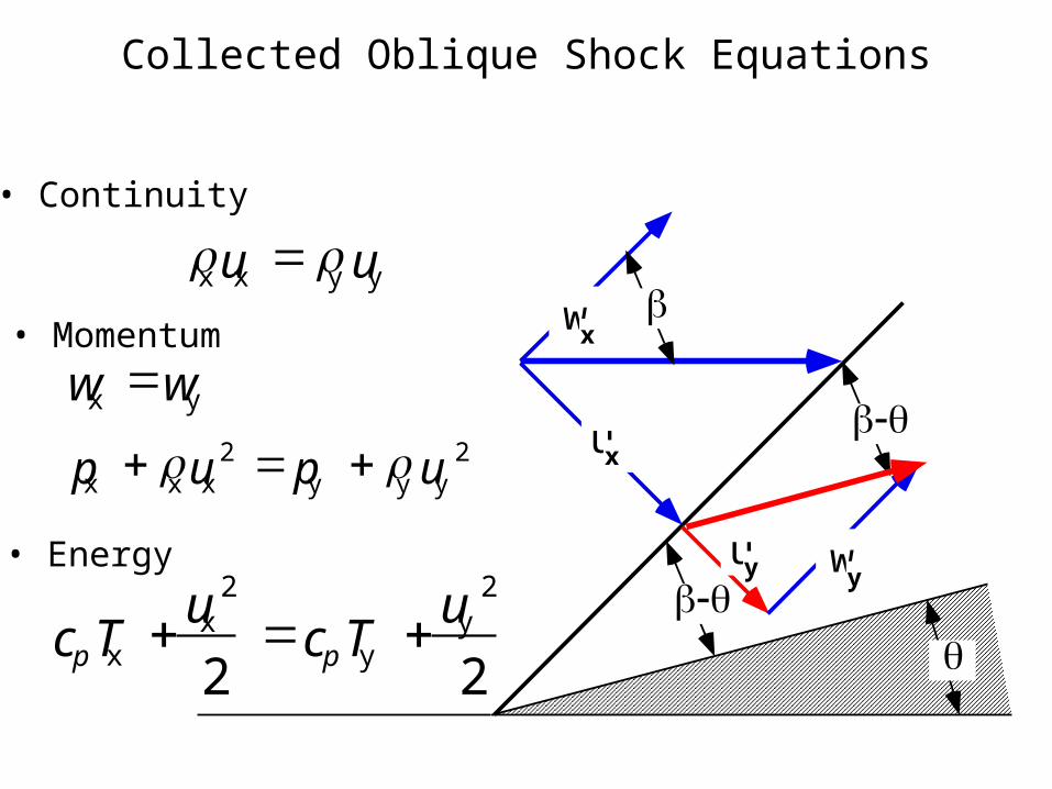
Collected Oblique Shock Equations

• Continuity

wx wy

px x ux

2 py

y uy2

x ux y uy

cpTx ux2

2cpTy uy

2

2

ux

uy

wx

wy

• Momentum

• Energy

w x &

M tx

ux &

Mnx

Vx & Mx

Vx & Mx

V y & M y

w y &

M ty

uy &

Mny

Vy & My

• Defining:

Mnx=Mxsin(

Mtx=Mxcos(

• Then by similarity we can write the solution

12

2)1(2

22

nx

nxny

M

MM

• Similarity Solution Letting

1

12 2

nx

x

y M

p

p

Mnx= Mxsin(

22

22

1

1221

nx

nxnx

x

y

M

MM

T

T

21

12

2

nx

nx

x

y

M

M

• Properties across an Oblique Shock wave ~ f(Mx, )

1

1sin2 2

x

x

y M

p

p

22

22

sin1

1sin22sin1

x

xx

x

y

M

MM

T

T

2sin1

sin12

2

x

x

x

y

M

M

Total Mach Number Downstream of Oblique Shock

w1 w2

Tangential velocity isConstant across obliqueShock wave

w1 w2 Mt1c1 Mt2c2 M1 cos()c1

Mt2 M1 cos()c1

c2

M1 cos()T1

T2

M 2 Mt22 Mn2

2

Tangential velocity isConstant across obliqueShock wave

M 2 Mt22 Mn2

2 Mn2 1

1 2

M1 sin( ) 2

M1 sin( ) 2 1

2

M 2 M1 cos( ) 2 T1

T2

1

1 2

M1 sin( ) 2

M1 sin( ) 2 1

2

Tangential velocity is Constant across oblique Shock wave

• Or … More simply .. If we consider geometric arguments

M 2 Mn2

sin

M3M2

Mn2Mt2

Oblique Shock Wave Angle

• Properties across Oblique Shock wave ~ f(M1, )

• is the geometric angle that “forces” the flow

• How do we relate to

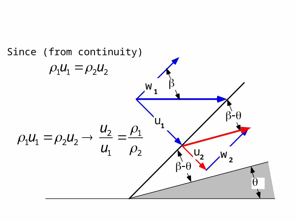
• Since (from continuity)

1u1 2u2

u1

u2

w1

w2

1u1 2u2 u2

u1

1

2

Oblique Shock Wave Angle (cont’d)

u1

u2

w1

w2

u2

w2

tan

u1

w1

tan

• from Momentum

w1 w2

Oblique Shock Wave Angle (cont’d)

• Solving for the ratio u2/u1

Implicit relationship for shock angle in terms ofFree stream mach number and “wedge angle”

u2

u1

tan

tan 1

2

2

1

1 Mn1

2

2 1 Mn12

tan

tan 2 1 M1 sin

2 1 M1 sin

2

• Solve explicitly for tan()

tan tan tan tan2 tan

2 1 M1 sin 2

1 M1 sin 2

tan

tan 1 M1 sin

2 2 1 M1 sin 2

1 M1 sin 2 tan2 2 1 M1 sin

2

Oblique Shock Wave Angle (cont’d)

• Simplify Numerator

tan 1 M1 sin 2 2 1 M1 sin

2

tan M1 sin 2 M1 sin

2 2 M1 sin

2 M1 sin

2

tan 2 M1 sin 2 1

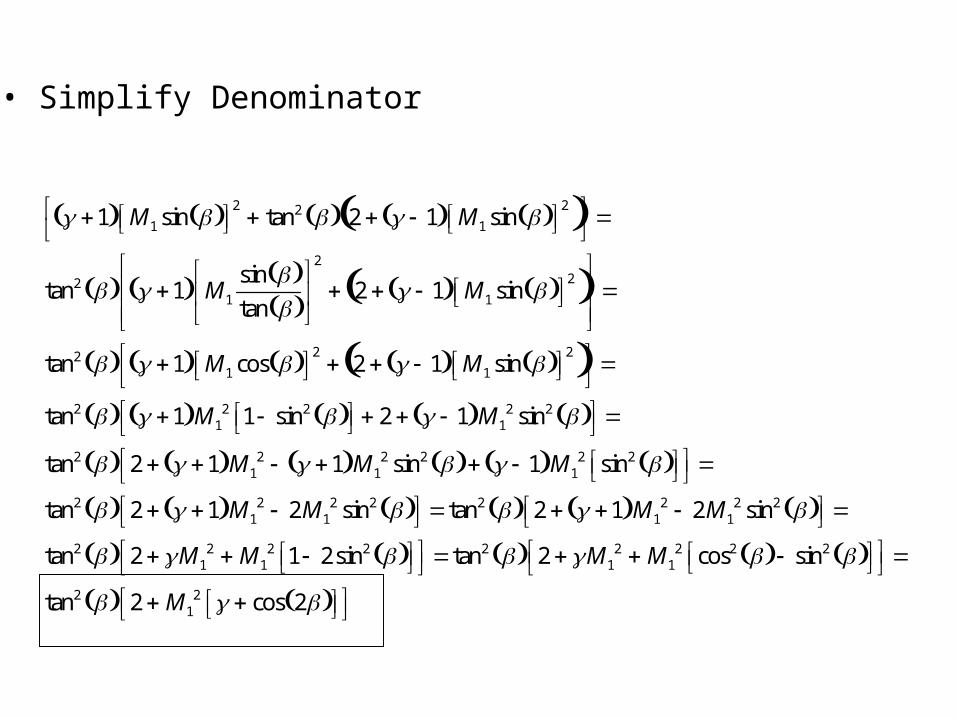
• Simplify Denominator

1 M1 sin 2 tan2 2 1 M1 sin

2

tan2 1 M1

sin tan

2

2 1 M1 sin 2

tan2 1 M1 cos 2 2 1 M1 sin

2

tan2 1 M12 1 sin2 2 1 M1

2 sin2

tan2 2 1 M12 1 M1

2 sin2 1 M12 sin2

tan2 2 1 M12 2M1

2 sin2 tan2 2 1 M12 2M1

2 sin2

tan2 2 M12 M1

2 1 2sin2 tan2 2 M12 M1

2 cos2 sin2

tan2 2 M12 cos 2

Oblique Shock Wave Angle (cont’d)

• Collect terms

tan 2 tan M1 sin

2 1

tan2 2 M12 cos 2

2 M1

2 sin2 1 tan 2 M1

2 cos 2 • “Wedge Angle” Given explicitly as function of shock angle and freestream Mach number

• Two Solutions “weak” and “strong” shock wave. In reality weak shock typically occurs;

strong only occurs under very Specialized circumstances .e.g near stagnation point for a detached Shock.

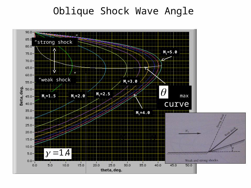
Oblique Shock Wave Angle

M1=1.5 M1=2.0 M1=2.5

M1=3.0

“strong shock”

“weak shock”

M1=4.0

M1=5.0

1.4

max

curve

Limiting Cases of Oblique Shock Wave

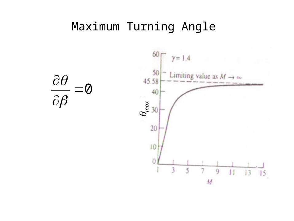
Maximum Turning Angle

0

max

High Angle Objects

max

max

Weak And Strong Oblique Shock

Supersoinc Intakes

Solving for Oblique Shock Wave Angle in Terms of Wedge Angle

• As derived

• “Wedge Angle” Given explicitly as function of shock angle and freestream Mach number

• For most practical applications, the geometric deflection angle (wedge angle) and Mach number are prescribed .. Need in terms of and M1

• Obvious Approach …. Numerical Solution using Newton’s method

tan 2 M1

2 sin2 1 tan 2 M1

2 cos 2

Solving for Oblique Shock Wave Angle in Terms of Wedge

Angle (cont’d)• Newton method

2 M12 sin2 1

tan 2 M12 cos 2

tan f () 0

f () f (( j ) ) f

( j )

( j ) O( 2 ) ....

( j1) ( j )

2 M12 sin2 1

tan 2 M12 cos 2

tan

f

( j )

Solving for Oblique Shock Wave Angle in Terms of Wedge

Angle (cont’d)• Newton method (continued)

• Iterate until convergence

f

2 M14 sin2 1 cos 2 M1

2 2 cos 2 1 2 sin2 2 M1

2 cos 2 2

Solving for Oblique Shock Wave Angle in Terms of Wedge

Angle (cont’d)

f

• “Flat spot”Causes potentialConvergence Problems withNewton Method

IncreasingMach

Solving for Oblique Shock Wave Angle in Terms of Wedge

Angle (cont’d)• Newton method … Convergence can often be slow (because of low derivative slope)

• Converged solution

true 60.26o

Solving for Oblique Shock Wave Angle in Terms of Wedge

Angle (concluded)• Newton method … or can “toggle” to strong shock solution

• Strong shock solution

strong 71.87o

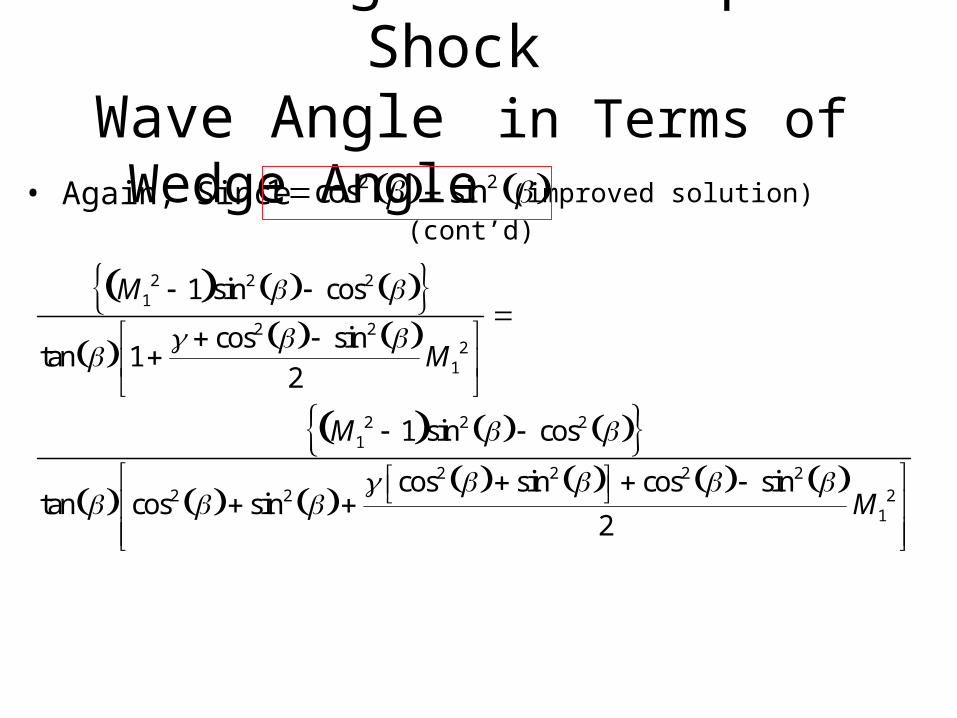
Solving for Oblique Shock Wave Angle in Terms of Wedge

Angle (improved solution)• Because of the slow convergence of Newton’s method for this implicit function… explicit solution … (if possible) .. Or better behaved .. Method very desirable

tan 2 M1

2 sin2 1 tan 2 M1

2 cos 2

2 M12 sin2 1

tan 2 M12 M1

2 cos2 sin2

cos 2 cos2 sin2 Substitute

Solving for Oblique Shock Wave Angle in Terms of Wedge

Angle (improved solution)

(cont’d)• But, since 1 cos2 sin2

2 M12 sin2 1

tan 2 M12 M1

2 cos2 sin2

2 M12 sin2 sin2 cos2

tan 2 M12 M1

2 cos2 sin2

Solving for Oblique Shock Wave Angle in Terms of Wedge

Angle (improved solution)

(cont’d)• Simplify and collect terms2 M1

2 sin2 sin2 cos2 tan 2 M1

2 M12 cos2 sin2

M12 1 sin2 cos2

tan 12

M12

1

2M1

2 cos2 sin2

M12 1 sin2 cos2

tan 12

M12

1

2M1

2 cos2 sin2

M12 1 sin2 cos2

tan 1 cos2 sin2

2M1

2

Solving for Oblique Shock Wave Angle in Terms of Wedge

Angle (improved solution)

(cont’d)• Again, Since

M12 1 sin2 cos2

tan 1 cos2 sin2

2M1

2

M12 1 sin2 cos2

tan cos2 sin2 cos2 sin2 cos2 sin2

2M1

2

1 cos2 sin2

Solving for Oblique Shock Wave Angle in Terms of Wedge

Angle (improved solution)

(cont’d)• Regroup and collect terms

M12 1 sin2 cos2

tan cos2 sin2 cos2 sin2 cos2 sin2

2M1

2

M12 1 tan2 1

tan 1 tan2 1 tan2 1 tan2

2M1

2

M12 1 tan2 1

tan 1 1

2M1

2 tan2 tan2 tan2

2M1

2

M12 1 tan2 1

tan 1 1

2M1

2

tan2 1

1

2M1

2

Solving for Oblique Shock Wave Angle in Terms of Wedge

Angle (improved solution)

(cont’d)• Finally

• Regrouping in terms of powers of tan()

tan M1

2 1 tan2 1 1

1

2M1

2

tan 1 1

2M1

2

tan3

1 1

2M

1

2

tan

tan3 1 1

2M

1

2

tan

tan M1

2 1 tan2 1 0

Solving for Oblique Shock Wave Angle in Terms of Wedge

Angle (improved solution)

(cont’d)• Letting

• Result is a cubic equation of the form

a 1 1

2M1

2

tan

b M12 1

c 1 1

2M1

2

tan

x tan

ax3 bx2 cx 1 0

• Polynomial has 3 real rootsi) weak shockii) strong shockiii) meaningless solution

( < 0)

Solving for Oblique Shock Wave Angle in Terms of Wedge

Angle (improved solution)

(cont’d)• Numerical Solution of Cubic (Newton’s method)

ax3 bx2 cx 1 f (x) 0

0 f (x j ) f (x)

x j

x j1 x j o(x2 )

x j1 x j f (x j )

f (x)

x j

x j ax j

3 bx j2 cx j 1

3ax j2 2bx j c

Solving for Oblique Shock Wave Angle in Terms of Wedge

Angle (improved solution)

(cont’d)• Collecting terms

x j ax j

3 bx j2 cx j 1

3ax j2 2bx j c

3ax j3 2bx j

2 cx j ax j3 bx j

2 cx j 1 3ax j

2 2bx j c

2ax j3 bx j

2 1

3ax j2 2bx j c

Solving for Oblique Shock Wave Angle in Terms of Wedge

Angle (improved solution)

(cont’d)• Solution Algorithm (iterate to convergence)

x j1 2ax j

3 bx j2 1

3ax j2 2bx j c

• Where again a 1 1

2M1

2

tan

b M12 1

c 1 1

2M1

2

tan

x tan

Solving for Oblique Shock Wave Angle in Terms of Wedge

Angle (improved solution)

(cont’d)• Properties of Solver algorithm are much improved

Improved AlgorithmOriginal Algorithm

true 60.26o

• Original algorithm• Improved algorithm

Solving for Oblique Shock Wave Angle in Terms of Wedge

Angle (improved solution)

(cont’d)• Three Solutions always returned depending on start condition

Original Algorithm Improved Algorithmtrue 60.26o

• Weak Shock Solution

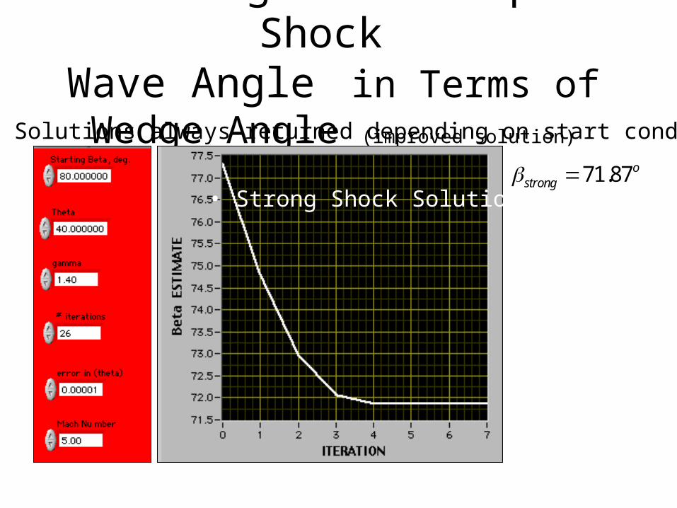
Solving for Oblique Shock Wave Angle in Terms of Wedge

Angle (improved solution)

(cont’d)• Three Solutions always returned depending on start condition

Improved Algorithm• Strong Shock Solutionstrong 71.87o

Solving for Oblique Shock Wave Angle in Terms of Wedge

Angle (improved solution)

(cont’d)• Three Solutions always returned depending on start condition

Improved Algorithm• Meaningless Solution meaningless 0o

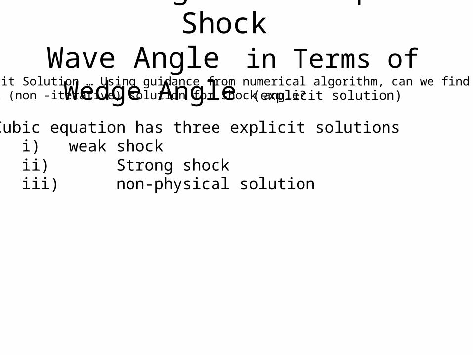
Solving for Oblique Shock Wave Angle in Terms of Wedge

Angle (explicit solution)

Improved Algorithm• Meaningless Solution

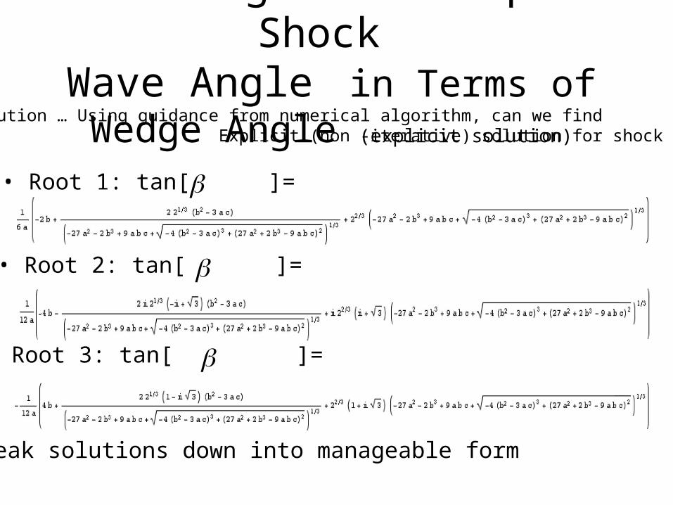
• Explicit Solution … Using guidance from numerical algorithm, can we findExplicit (non -iterative) solution for shock angle?

• Cubic equation has three explicit solutionsi) weak shockii) Strong shockiii) non-physical solution

Solving for Oblique Shock Wave Angle in Terms of Wedge

Angle (explicit solution)

Improved Algorithm

• Explicit Solution … Using guidance from numerical algorithm, can we find Explicit (non -iterative) solution for shock angle?

• Root 1: tan[]=

• Root 2: tan[]=

• Root 3: tan[]=

• Break solutions down into manageable form

Solving for Oblique Shock Wave Angle in Terms of Wedge

Angle (explicit solution)

Improved Algorithm• Meaningless Solution

• Explicit Solution (From Anderson, pp. 142,143) …

1 1

2M1

2

tan

tan3 M12 1 tan2 1

1

2M1

2

tan

tan 1 0

tan M1

2 1 2 cos4 cos 1

3

3 1 1

2M1

2

tan

M12 1 2

3 1 1

2M1

2

1 1

2M1

2

tan2

M1

2 1 3 9 1

1

2M1

2

1 1

2M1

2 1

4M1

4

tan2

3

= 0 ---> Strong Shock

= 1 ---> Weak Shock

Solving for Oblique Shock Wave Angle in Terms of Wedge

Angle (explicit solution)

Improved Algorithm• Meaningless Solution

• Explicit Solution Check … let {M=5, , =40

M12 1 2

3 1 1

2M1

2

1 1

2M1

2

tan2 =

= 13.5321

52 1 2

3 11.4 1

252+

11.4 1+

252+

180

40 tan

2

0.5

1.4

Solving for Oblique Shock Wave Angle in Terms of Wedge

Angle (explicit solution)

Improved Algorithm• Meaningless Solution

• Explicit Solution Check … let {M=5, , =40

=

M12 1 3

9 1 1

2M1

2

1 1

2M1

2 1

4M1

4

tan2

3

= -0.267118

52 1 3

9 11.4 1

252+

11.4 1

252 1.4 1+

454+ +

180

40 tan

2

13.53213

1.4

Solving for Oblique Shock Wave Angle in Terms of Wedge

Angle (explicit solution)

Improved Algorithm• Meaningless Solutiontan

M12 1 2 cos

4 cos 1 3

3 1 1

2M1

2

tan

= 1 ---> Weak Shock

=

180

52 1 2 13.5321 4 1 0.26712 acos+

3 cos+

3 11.4 1

252+

180

40 tan

atan

= 60.259 Check!

• Explicit Solution Check … let {M=5, , =40 1.4

Solving for Oblique Shock Wave Angle in Terms of Wedge

Angle (explicit solution)

• Meaningless Solutiontan

M12 1 2 cos

4 cos 1 3

3 1 1

2M1

2

tan

= 0 ---> Strong Shock

=

= 71.869 Check!

180

52 1 2 13.5321 4 0 0.26712 acos+

3 cos+

3 11.4 1

252+

180

40 tan

atan

… OK .. This works and isClearly the Best method

(concluded)

• Explicit Solution Check … let {M=5, , =40 1.4

Oblique Shock Waves:Collected Algorithm

• Properties across Oblique Shock wave ~ f(M1, )

• is the geometric angle that “forces” the flow

tan 2 M1

2 sin2 1 tan 2 M1

2 cos 2

Oblique Shock Waves:Collected Algorithm (cont’d)

• Can be re-written as third order polynomial in tan()

• “Very Easy” numerical solution

1 1

2M

1

2

tan

tan3 1 1

2M

1

2

tan

tan M1

2 1 tan2 1 0

x j1 2ax j

3 bx j2 1

3ax j2 2bx j c

a 1 1

2M1

2

tan

b M12 1

c 1 1

2M1

2

tan

x tan

• Cubic equation has three solutionsi) weak shockii) Strong shockiii) non-physical solution

Oblique Shock Waves:Collected Algorithm (cont’d)

• “Less Obvious” explicit solution

tan M1

2 1 2 cos4 cos 1

3

3 1 1

2M1

2

tan

M12 1 2

3 1 1

2M1

2

1 1

2M1

2

tan2

M1

2 1 3 9 1

1

2M1

2

1 1

2M1

2 1

4M1

4

tan2

3

= 0 ---> Strong Shock

= 1 ---> Weak Shock

Oblique Shock Waves:Collected Algorithm (cont’d)

• ... and the rest of the story …

2

1

1 M1 sin 2

2 1 M1 sin 2 p2

p1

12

1 M1 sin 2 1

T2

T1

12

1 M1 sin 2 1

2 1 M1 sin 2 1 M1 sin 2

Oblique Shock Waves:Collected Algorithm (concluded)

• ... and the rest of the story …

Mn2 1

1 2

M1 sin 2

M1 sin 2 1

2

M 2 Mn2

sin

P02

P01

2

1 M1 sin 2

1 2

1

1 2

M1 sin

2

1 1

2M1 sin 2

1

Example:•M1 = 3.0, p1=1atm, T1=288K, =20=1.4,

M1

M2

• Compute shock wave angle (weak)

• Compute P02, T02, p2, T2, M2 … Behind Shockwave

Example: (cont’d)

•M1 = 3.0, p1=1atm, =1.4, T1=288K, =20

• Explicit Solver for

M12 1 2

3 1 1

2M1

2

1 1

2M1

2

tan2 =7.13226

M1

2 1 3 9 1

1

2M1

2

1 1

2M1

2 1

4M1

4

tan2

3=0.93825

Example: (cont’d)

•M1 = 3.0, p1=1atm, =1.4, T1=288K, =20

• = 1 (weak shock)

180

32 1 2 7.132264 1 0.93825 acos+

3 cos+

3 11.4 1

232+

180

20 tan

atan

tan M1

2 1 2 cos4 cos 1

3

3 1 1

2M1

2

tan

=

37.764

Example: (cont’d)

•M1 = 3.0, p1=1atm, =1.4, T1=288K, =20

• Normal Component of Free stream mach Number

p2

p1

12

1 Mn12 1

Mn1 M1 sin 3

18037.7636

sin =1.837

Normal Shock Solver

p2 = 3.771(1 atm) = 3.771 atm

• Compute Pressure ratio across shock

• Flow is compressed

Example: (cont’d)

•M1 = 3.0, p1=1atm, =1.4, T1=288K, =20

• Temperature ratio Across Shock

Normal Shock Solver

T2 = 1.5596(288 K) = 449.2 K

T2

T1

12

1 Mn12 1

2 1 Mn12

1 Mn12

Example: (cont’d)

•M1 = 3.0, p1=1atm, =1.4, T1=288K, =20

• Stagnation Pressure ratio across shock

Normal Shock Solver

0.7961

Mn1 M1 sin 3

18037.7636

sin =1.837

P02

P01

Example: (cont’d)

•M1 = 3.0, p1=1atm, =1.4, T1=288K, =20

• Stagnation Pressure ratio (alternate method)

P02

P01

2

1 Mn12

1 2

1

1 2

Mn12

2

1 1

2Mn1

2

1

2

1.4 1+ 1.4 3

18037.7636

sin

2 1.4 1 2

1

1.4 1

1.4 1+ 2

2

3

18037.7636

sin

2

11.4 1

2 3

180

37.7636 sin

2

+

1.4

1.4 1

=0.7961

Example: (cont’d)

•M1 = 3.0, p1=1atm, =1.4, T1=288K, =20

• Stagnation Pressure

=29.24 atm

P02 P02

P01

P01

p1

p1 P02

P01

1 1

2M1

2

1

p1

0.7961 11.4 1

232

1.4

1.4 11atm

Example: (cont’d)

•M1 = 3.0, p1=1atm, =1.4, T1=288K, =20

• Stagnation Temperature behind shock

=806.4 oK

T02 T01 T01

T1

T1 1 1

2M1

2

T1

11.4 1

232

288o K

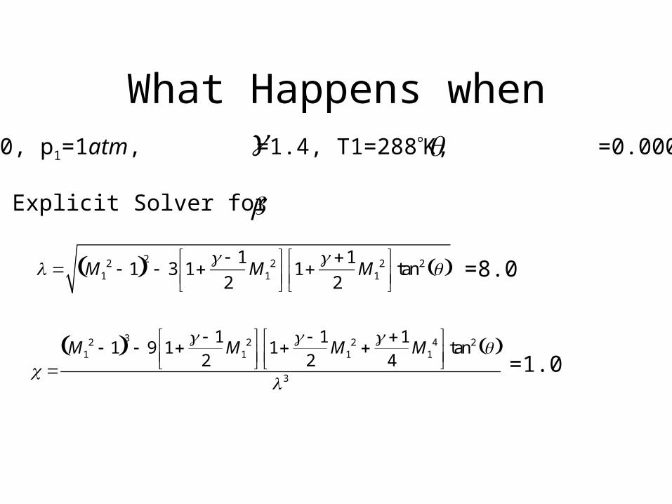
What Happens when•M1 = 3.0, p1=1atm, =1.4, T1=288K, =0.00001

• Explicit Solver for

M12 1 2

3 1 1

2M1

2

1 1

2M1

2

tan2 =8.0

M1

2 1 3 9 1

1

2M1

2

1 1

2M1

2 1

4M1

4

tan2

3=1.0

What Happens when (cont’d) •M1 = 3.0, p1=1atm, =1.4, T1=288K, =0.00001

tan M1

2 1 2 cos4 cos 1

3

3 1 1

2M1

2

tan

=19.47 180

sin 1 1

M1

19.47o

• “mach line”

What Happens when (cont’d) •M1 = 3.0, p1=1atm, =1.4, T1=288K, =0.00001

• Normal Component of Free stream mach Number

Mn1 M1 sin 1.0000

• p2

p1

12

1 Mn12 1 = 1.0 (NO COMPRESSION!)

Expansion Waves • So if>0 .. Compression around corner

=0 … no compression across shock

M1

M2

Expansion Waves (concluded) • Then it follows that

<0 .. We get an expansion wave

• Next

Prandtl-Meyer Expansion waves