An XFEM/CZM implementation for massively parallel simulations of composites fracture

Guillermo Viguerasa,b, Federico Sketa, Cristobal Samaniegoc, Ling Wud, Ludovic Noelsd, Denny Tjahjantoa,e, Eva Casonic,Guillaume Houzeauxc, Ahmed Makradif, Jon M. Molina-Aldareguiaa, Mariano Vazquezc, Antoine Jerusalema,g

aIMDEA Materials Institute, Getafe, SpainbIMDEA Software Institute, Madrid, Spain

cBarcelona Supercomputing Centre, Barcelona, SpaindUniversity of Liege, Liege, Belgium

eKTH Royal Institute of Technology, Stockholm, SwedenfCRP Henri Tudor, Luxembourg-Kirchberg, Luxembourg

gUniversity of Oxford, Oxford, UK

Abstract

Because of their widely spread use in many industries, composites are the subject of many research campaigns. More particularly,the development of both accurate and flexible numerical models able to capture their intrinsically multiscale modes of failure isstill a challenge. The standard finite element method typically requires intensive remeshing to adequately capture the geometry ofthe cracks and high accuracy is thus often sacrificed in favor of scalability, and vice versa. In an effort to preserve both properties,we present here an extended finite element method (XFEM) for large scale composite fracture simulations. In this formulation, thestandard FEM formulation is partially enriched by use of shifted Heaviside functions with special attention paid to the scalability ofthe scheme. This enrichment technique offers several benefits, since the interpolation property of the standard shape function stillholds at the nodes. Those benefits include (i) no extra boundary condition for the enrichment degree of freedom, and (ii) no needfor transition/blending regions; both of which contribute to maintain the scalability of the code.

Two different cohesive zone models (CZM) are then adopted to capture the physics of the crack propagation mechanisms. Atthe intralaminar level, an extrinsic CZM embedded in the XFEM formulation is used. At the interlaminar level, an intrinsic CZMis adopted for predicting the failure. The overall framework is implemented in ALYA, a mechanics code specifically developed forlarge scale, massively parallel simulations of coupled multi-physics problems. The implementation of both intrinsic and extrinsicCZM models within the code is such that it conserves the extremely efficient scalability of ALYA while providing accurate physicalsimulations of computationally expensive phenomena. The strong scalability provided by the proposed implementation is demon-strated. The model is ultimately validated against a full experimental campaign of loading tests and X-ray tomography analyses fora chosen very large scale.

Keywords:Composites, XFEM, Cohesive elements, Failure, Large scale parallel simulations

1. Introduction

The prediction of structural failure in laminated compos-ites is particularly challenging since both intra and interlaminarfailure mechanisms (highly multiscale in nature) contribute tothe fracture process [1]. Indeed, a full understanding of frac-ture mechanisms in composites requires an approach linkingmicroscale deformation features within a ply to its macroscalelaminate counterpart. One way to predict mesoscale fracturefrom numerical simulations is to analyze the microscale defor-mation mechanisms with constitutive models accounting for thefracture processes ranging from micro-crack initiation to meso-crack propagation. A natural way to achieve this goal is to en-rich the finite element model with the so-called cohesive zonemethod (CZM).

Email address: antoine.jerusalem@eng.ox.ac.uk (AntoineJerusalem)

The CZM [2, 3] defines a traction between crack lips dur-ing the separation process, which is modeled using a tractionseparation law (TSL). Figures 1a and 1b show two examplesof cohesive laws. In both laws, the TSL curve eventually de-creases monotonically until reaching zero at a critical openingdisplacement δc to model a progressive damage of the material.The energy dissipated during this process corresponds to thefracture energy Gc. The TSL for quasi-brittle materials is thusrelated to the breaking of atomic bonds which is characterizedby two physical parameters: the material strength σc and thefracture energy Gc.

In most of the finite element applications of the CZM, thecohesive elements are inserted at the beginning of the simu-lation, in which case the TSL is decomposed into an initialloading phase, followed by an unloading phase once the stressreaches the material strength σc (see Figure 1a). Depending onthe model, the unloading can either be reversible or irreversiblein case of closure of the crack. Such approach is attractive as it

Preprint submitted to Composite Structures December 18, 2014

can easily be implemented, in particular when the crack path iswell defined, e.g. for composite delamination [4, 5]. This so-called “intrinsic” cohesive law has thus extensively been used tomodel fracture in the matrix phase of composites [6] or to pre-dict the interaction between intralaminar and interlaminar fail-ure mechanisms by inserting cohesive elements in-between allbulk elements [7, 8]. However, such scheme exhibits a strongmesh dependency, alters the structural stiffness and adds spuri-ous stiffness elements in a mesh dependent way, since the ini-tial slope in the reversible part of the TSL does not satisfy theconsistency condition. Some authors have tried to mitigate thisproblem by increasing the initial slope of the TSL [4, 9, 10],but this technique leads to an ill-conditioned stiffness matrix forstatic simulations or to unacceptable small values of the criticaltime step for explicit dynamic simulations [11].

In order to avoid the drawbacks inherent to the intrinsic ap-proach, an “extrinsic” cohesive law accounting exclusively forthe irreversible phase can be used [12, 13], see Figure 1b. Prac-tically a simulation using such scheme proceeds with a classicalfinite element approach and cohesive elements are introduced atthe interface of bulk elements at the onset of fracture. Althoughthe 3D implementation of this framework [14] is not straight-forward due to the mesh topology changes during the compu-tation, it predicts crack propagation with an energy and a crackpath that both converge with the mesh size, as shown by Ariaset al. [15] and by Molinari et al. [16]. However the implemen-tation complexity increases drastically for parallel framework[17] and can suffer from low scalability unless a graph-basedinternal structure is used [18, 19].

The difficulties presented by the extrinsic CZM and the lim-itations of the CZM in its intrinsic form, where a scalable ap-plicability is reduced to cases for which the crack path is welldefined, have led some authors to propose hybrid models com-bining the use of CZM with some numerical methods for simu-lating damage processes. Research efforts have thus focused oncombining intrinsic cohesive elements for delamination, withcontinuum damage models for ply damage [20, 21, 22]. Al-though this mesomechanical approach has proved to be suc-cessful for some structural configurations [20], the use of twodifferent kinematic representations for interlaminar and intralam-inar failure presents some fundamental problems. For exam-ple, in the modeling of the interaction between transverse ma-trix cracks and delamination it is necessary to capture the highstresses at the tip of the transverse crack. However, a me-somechanical model cannot possibly capture this interactionbecause the elements where the transverse crack is predictedsoften without being able to accurately capture the stress fieldat the interface.

Some other approaches have suggested hybrid discontinu-ous Galerkin (DG)/CZM approaches [23, 24, 25]. The mainfeature of the DG method for non-linear solid mechanics isits ability to take into account discontinuities of the unknownfield between bulk elements [26, 27, 28, 29, 30]. With the hy-brid DG/CZM method, interface elements are therefore insertedbetween bulk elements at the beginning of the simulation andcontinuity during the pre-fracture stage is ensured by havingrecourse to the consistent DG interface terms. An extrinsic co-

hesive law can thus be integrated on the already existing inter-face elements once a fracture criterion is met, without requiringmesh topology changes. This approach has been successfullyimplemented in a 3D parallel framework for micro-meso simu-lation of intralaminar fracture in composites [31]. The methodhas also been used in 2D to study the effect of the fibers shapeson the composite resistance [25]. Such an approach has alsobeen developed for thin homogeneous elastic bodies [32, 33]and for thin homogeneous elasto–plastic structures [34]. How-ever, similarly to the simple CZM approach, the discontinu-ities defined by the DG/CZM approach suffer from mesh de-pendency. It might thus be adequate for interlaminar failuresimulations, but not for intralaminar failure.

In order to alleviate the mesh-dependency inherent to theintrinsic cohesive approach, the eXtended (or Generalized) Fi-nite Element Method (XFEM) [35] has been used in combi-nation with CZM [36, 37] for predicting fracture mechanisms.XFEM offers the possibility to represent the entire crack ge-ometry independently of the mesh, so that refined meshes arenot necessary to model crack growth. Also, XFEM exploitsthe partition-of-unity property of finite elements [38], which al-lows local enrichment functions to be easily incorporated intoa finite element approximation. A standard approximation isthus enriched in a region of interest by the local functions inconjunction with additional degrees of freedom. For the pur-pose of fracture analysis, the enrichment functions are the near-tip asymptotic fields and a discontinuous function to representthe jump in displacement across the crack line. These featuresmake XFEM an attractive method for fracture prediction sinceit can flexibly represent the crack path without prior knowledgeof the orientation of the crack plane.

Due to its multiscale nature, the simulation of delamina-tion and ply failure results in high computational requirementswhich solid mechanics codes traditionally do not manage effi-ciently. Most of the commercial codes cannot efficiently scalein parallel computers when more than hundreds of cores areused (this is especially true when using implicit solvers). Aca-demic codes, on the other hand, have often relied on the needto develop one unique technique of interest for their develop-ment, potentially followed by a secondary development phaseaimed at scaling it up because of the prohibitive cost of the tech-nique. Led by the Barcelona Supercomputing Center (BSC-CNS), Alya [39, 40], on the contrary, has been conceived fromthe beginning as a massively large scale computational me-chanics code aimed at solving Partial Differential Equations(PDEs) in non-structured meshes. Alya exploits the similari-ties of the PDE-governed problems to solve with high paral-lel performance (thousands of cores) compressible and incom-pressible flows, solid mechanics, thermal flows, excitable me-dia or quantum mechanics for transient molecular dynamics[41, 42, 43, 44, 40]. Parallelization is hidden behind a com-mon solver that assembles matrices and residuals and carriesout the solution scheme. The scalability of the code thus ex-clusively depends on one unique set of parallel communicationsubroutines independently of the physics of the problem.

We thus propose herein an Alya-implementation of XFEMfor the simulation of fracture in laminated composite materials.

2

∆

t

GC

∆c

σc

(a) Intrinsic

∆

t

GC

∆c

σc

(b) Extrinsic

Figure 1: Cohesive laws

In this approach, the intrinsic CZM is used to model interlam-inar fracture, whereas XFEM is combined with the extrinsicCZM to model intralaminar fracture. The models are imple-mented so as to conserve the extreme scalability of Alya whileensuring the accurate physical description of the material defor-mation and failure. The details of this scalable implementationare thoroughly described.

The implementation is ultimately validated against experi-mental open hole tensile tests of laminated carbon fiber rein-forced polymers (CFRP) where damage has been thoroughlycharacterized by X-ray computed tomography (XCT). XCT pro-vides actual 3D information of the damage and microstructurein every ply from a number of X-ray radiographies obtained atdifferent angles in a non-destructive manner. In addition, con-trast enhancement was obtained by infiltrating a liquid with ahigh X-ray absorption coefficient (e.g. ZnI), leading to a com-plete characterization of damage by matrix cracking and in-terply delamination [45, 46]. While the damage mechanismsin fiber reinforced polymers are qualitatively well documentedin the literature [47, 48, 49, 50, 51, 52], quantitative data onthe evolution of matrix cracking and interply delamination withstrain is less common [53]. Traditionally, quantitative charac-terization has been limited by time consuming and destructiveserial sectioning microscopy methods or to simpler laminate se-quences due to the inability of X-ray radiography to separatethe contribution from different plies [54, 53]. These limitationsare overcome by XCT, which has been used in this work tofollow the development of damage of each individual ply of[90/ + 45/ − 45/90/0]s carbon fiber laminates during the ten-sile deformation. The evaluation was focused on the evolutionof crack density and delamination as a function of strain, fordirect comparison with the simulation results, which show anexcellent agreement.

Section 2 presents the numerical scheme implemented inAlya and Section 3 focuses on implementation specificities re-quired to conserve both the robustness and scalability of Alya.The experimental campaign, i.e. materials mechanical and XCT

characterization, is provided in Section 4. The results are dis-cussed in Section 5, and the conclusions of this work are finallygiven in Section 6.

2. Numerical Scheme

This section describes the standard Galerkin formulationwith XFEM enrichment of the solution, and the cohesive lawsused for the inter- and intralaminar fracture models. Implemen-tation details of the discretization and integration are also de-scribed. See Ref. [23, 24, 31] for more details.

2.1. Enrichment of solution approximationLet X ∈ B0 be a material point in the reference configu-

ration, and x = ϕ(X) ∈ B be the corresponding point in thedeformed configuration, where ϕ is the deformation function.The deformation gradient tensor F is defined as

F = Grad x . (1)

In a Cartesian basis the components of F are given by

FiJ =∂xi

∂XJ. (2)

Let the undeformed body B0 be approximated by a domainΩ0 ≈ B0, where Ω0 is subdivided into a set of triangular ele-ments Ωe

0, such that Ω0 =⋃

e Ωe0.

Recall that in a standard finite element method, the solutionapproximation of nodal displacement u = x − X can be writtenas

u(X) ≈ uh(X) =∑a∈I

Na(X)ua , (3)

where I is the set of nodes a supporting the domain Ω0, andNa is the shape function corresponding to the nodal support a.In a finite element discretization, Na is chosen such that it has acompact support on node a, i.e. Na(Xa) = 1 and Na(Xb) = 0 forall b , a. Therefore, the above solution approximation satisfiesthe Kronecker-delta or interpolation property, ua = uh(Xa).

3

In order to account for discontinuities, the solution approx-imation (3) is enriched using additional interpolation functionscapturing the discontinuities (or sharp gradients). Let ψ(X) bean enrichment function, such that the enriched solution approx-imation can be written as

uh(X) =∑a∈I

Na(X)ua +∑a∈I

f a(X)ψ(X)αa , (4)

where αa is the vector of additional unknowns or degrees offreedom associated with the enriched solution for node a, andwhere f a(X) is the corresponding interpolation function thatsatisfies the partition-of-unity property, i.e.∑

a∈I

f a(X) = 1 . (5)

For simplicity, the partition-of-unity function f a is chosen tobe the same as the standard finite element shape function, i.e.f a = Na. The expression for the enriched approximation of thedisplacement field thus reads as

uh(X) =∑a∈I

Na(X) (ua + ψ(X)αa) . (6)

Cracks are growing open interfaces and can thus be rep-resented by two level set functions Φ and Λ, describing re-spectively the path of the crack and the position of the cracktip(s)/edge(s), such that Γ0c = X |Φ(X) = 0 and Λ(X) ≤ 0.In this case, the level set function Φ can be described using asigned-distance function as follows:

Φ(X) = ‖X − XΓ‖ sign (nΓ · (X − XΓ)) , (7)

for all X ∈ Ω0, where XΓ is the projection of X on the crackpath Γ0c and nΓ is a vector normal (with a continuous orienta-tion along the crack path) to the path at point XΓ. Meanwhile,the level set function Λ(X) is constructed such that its path isorthogonal/perpendicular to the path of Φ(X) at the crack tip(s).

Note that special treatments need to be introduced to dealwith singularity at the crack tip. Such approaches generally in-clude additional enrichment functions at the crack tip based onthe elastic fracture mechanics model in order to deal with thesingularity associated with the crack tip. Alternatively, the co-hesive law model typically used in quasi-brittle and ductile ma-terials can be used to solve both the crack opening and the cracktip singularity problem without additional enrichment [55]. More-over in the cohesive crack approach, cracks are virtually ex-tended up to the edge of the partitioned elements, such thatlocally (element-wise), the crack path can be considered as aclosed interface. More details on the cohesive crack model willbe presented in Section 2.3.

Assuming closed interfaces at the element level, the Heavi-side enrichment function H for fully partitioned elements (withΛ ≤ 0) is given by

ψ(X) = H(Φ(X)) =

1 ∀Φ(X) > 0 ,0 ∀Φ(X) < 0 , (8)

as illustrated in Figure 2a. The effective enrichment functionof node a is then obtained by Na(X)H(X), see Figure 2b. How-ever, the above enrichment function does not satisfy the Kronecker-delta (or interpolation) property at nodes:

uh(Xa) = ua + H(Xa)αa , ua . (9)

To overcome this issue, a shifted Heaviside function Ha(X) =

H(X) − H(Xa) is applied in place of the original Heaviside en-richment function, such that the enriched solution approxima-tion of Equation (6) reads [55]:

uh(X) =∑a∈I

Na(X)(ua + Ha(X)αa

). (10)

The enriched solution approximation in Equation (10) guaran-tees the interpolation property of diplacement uh(Xa) = ua,whereas the effective jump in the displacement field across thecrack path Γ0c is given by Juh(X)K =

∑a∈I Na(X)αa, for all

X ∈ Γ0c, as indicated in Figure 2d.Because the effect of discontinuity is local within a limited

region around the crack, Heaviside enrichments can be appliedpartially, i.e. only on a particular domain Ω0c ⊂ Ω0 in the neigh-borhood of the crack path Γ0c. Another advantage of this for-mulation is that there is no need for special treatments in theblending/transition elements situated in-between enriched andnon-enriched elements: the elements in the transition regioncan be treated as standard elements. Indeed, smooth transitionbetween the displacement unknowns of the enriched elementand of the standard elements is guaranteed, thanks to the inter-polation property of the shifted shape function, ua = uh(Xa).Note that blending elements could potentially still be needed inother situations, such as general stress intensity factor calcula-tions.

2.2. Governing equationsThe equation of balance of momentum with respect to the

reference configuration can be written as

Div P + b0 = ρ0u , ∀X ∈ B0 , (11)

where ρ0 is the mass density (with respect to the reference vol-ume) and Div is the divergence operator with respect to the ref-erence configuration. Tensor P and vector b0 stand for, respec-tively, the first Piola–Kirchhoff stress and the distributed bodyforce on the undeformed body. Prescribed displacements andtractions are applied on the reference boundary Γ0 = Γd0 ∪ Γn0,where Γd0 and Γn0 correspond to the Dirichlet and Neumannboundary conditions, respectively, as follows:

u = u , ∀X ∈ Γd0 , (12)P · n0 = t0 , ∀X ∈ Γn0 . (13)

where n0 is the normal to the reference surface at the corre-sponding boundary.

The weak form of balance of the momentum Equation (11)can be formulated as∫

B0

Div P · w dV0 +

∫B0

b0 · w dV0 =

∫B0

ρ0u · w dV0 . (14)

4

(a) Standard FE shape functions

Φ = 01

3

N1(X)

2

N2(X)N3(X)

Φ < 0

Φ > 0Ωe

0

(b) Heaviside function for crack

Φ = 01

3 2

H(Φ(X),Λ(X))

Ωe0

(c) FE enrichment functions by heaviside

Φ = 01

3N1(X)H(X)

2

N2(X)H(X)N3(X)H(X)

Ωe0

(d) FE enrichment functions with shifting

Φ = 013 2

Ωe0

N1(X)H(X)–H(X1)

N2(X)H(X)–H(X2)N3(X)H(X)–H(X3)

nΓ

Figure 2: Finite element shape functions Na(X) and the enriched functions Na(X)ψ(X) using Heaviside function as enrichment

for any arbitrary admissible virtual displacement w.By making use of the finite element approximation of the

enriched solution (see Equation (10)) for both the discretizedsolution and the discretized virtual displacement, the XFEMformulation for the balance of momentum Equation (14) thusreads as follows: find the vector of unknowns z made of allua ∈ R3 and αa ∈ R3 of all nodes a such that:[

Muu MuαMαu Mαα

]· z +

(fint,ufint,α

)=

(fext,ufext,α

), (15)

where Muu, Muα, Mαu, Mαα, fint,u, fint,α, fext,u and fext,α are,respectively, the mass matrices, vectors of internal and externalforces for the unknown displacements and additional degreesof freedom, along with the cross-terms for the mass matrices.These quantities are constructed and assembled from the corre-sponding element quantities Me

uu, Meuα, Me

αu, Meαα, f e

int,u, f eint,α,

f eext,u and f e

ext,α, which are the corresponding mass matrix, in-ternal force vector and external force vectors.

In the above expression, the components Me,iakbuu , Me,iakb

uα ,Me,iakbαu , and Me,iakb

αα of the elementary mass matrix are given by

Me,iakbuu =

∫Ωe

0

ρ0δikNaNbdV0 ,

Me,iakbuα =

∫Ωe

0

ρ0δikNa(NbHb)dV0 ,

Me,iakbαu =

∫Ωe

0

ρ0δik(NaHa)NbdV0 ,

Me,iakbαα =

∫Ωe

0

ρ0δik(NaHa)(NbHb)dV0 .

(16)

where δik is the Kronecker symbol. The components f e,iaint,u and

f e,iaint,α of the elementary internal force vector are given by

f e,iaint,u =

∫Ωe

0

PiJ Na,JdV0 ,

f e,iaint,α =

∫Ωe

0

PiJ HaNa,JdV0 +

∫Γe

0c

tci NadS 0 ,

(17)

where tc is the traction at the crack surface1. The componentsof the external force vector f e,ia

ext,u and f e,iaext,α are given by

f e,iaext,u =

∫Γe

0t

t0iNadS 0 +

∫Ωe

0

b0iNadV0 ,

f e,iaext,α =

∫Γe

0t

t0i(NaHa)dS 0 +

∫Ωe

0

b0i(NaHa)dV0 .

(18)

The spatial integration in the equations above are done byGauss quadrature. In the case of a cracked element, the elementis cut by a planar interface. This partition results in a failure ofthe standard Gauss quadrature integration method, as there is noguarantee to have at least one Gauss point on each side of thecrack. In order to solve this issue, the element is decomposedinto subelements. For example, a cracked tetrahedron is splitinto a tetrahedral and a pentahedral subelement, in turn subdi-vided into tetrahedral elements, whereas a cracked hexahedroncan be split into a combination of prisms and hexahedra. Thenumerical integrations on the partitioned element can then beperformed using standard Gauss quadrature over the (smoothand continuous) subelements.

In addition, to evaluate the integrals over surfaces/paths Gaussintegration points are also defined on surfaces/boundaries. This

1Note that Nanson’s formula should actually be used to relate the tractionin the current configuration to the one in the reference configuration. However,matrix cracking almost exclusively occurs at small strain, thus justifying theapproximation.

5

is specifically the case when evaluating cohesive traction onthe crack surface, or when applying Neumann boundary condi-tions. Due to the formation of interfaces (or cracks), additionalGauss integration points are also defined on the (partitioning)interface Γ0c (which is a triangle for tetrahedral elements, oreither a triangular or a quadrilateral element for hexahedral el-ements).

Finally, the time integration of Equation (15) is done by useof the explicit form of the generalized Newmark algorithm, seeRef. [40] for more details.

2.3. Constitutive modelAs commonly done, simple orthotropic linear elasticity (with

adequate rotation with respect to the fiber orientation) is usedfor the bulk constitutive model, with fiber orientation specificto each ply. This section thus focuses on the interlaminar andintralaminar failure constitutive models. The formulations ofthe proposed models are briefly summarized in the following,see Camacho and Ortiz [12] for more details.

Both models define the traction–separation law, tc(δΓ), whichis required in order to describe the evolution of cohesive crack.The jump/discontinuity in the displacement field (crack open-ing) δΓ is obtained from

δΓ(X) = Juh(X)K =∑a∈Ic

Na(X)αa , (19)

for all X ∈ Γ0c, where the crack surface is Γ0c defined by Ic, asubset of I.

A scalar representing the effective opening of displacementδΓ can be defined as

δΓ =

√λ2(δΓ,s)2 + (δΓ,n)2 . (20)

where λ determines the effective contribution/weight of the normof the sliding/tangential component δΓ,s of the displacementopening with respect to the norm of its normal component δΓ,n.The interface traction tc corresponding to the above effectivedisplacement opening can then be expressed as

tc =tc

δΓ

(λ2δΓ,ssΓ + δΓ,nnΓ

), (21)

where tc is a scalar representing the effective interface traction,and where sΓ and nΓ are the local tangential and normal basisvectors on the crack surface.

2.3.1. Interlaminar failureThe Rose–Ferrante intrinsic cohesive law is used to model

the interlaminar delamination process [13]. The correspondingelements are introduced from the beginning as a preprocessingsteps. This choice is rationalized by the fact that the delamina-tion is expected to occur between the plies. This intrinsic lawdescribes the envelope of the relation between the effective trac-tion tc and the corresponding effective displacement separationδΓ upon loading (or crack opening):

tc = etcritδΓ

δcritexp

(− δΓ

δcrit

), if δΓ = δmax and ˙δΓ ≥ 0 , (22)

where e = exp(1), tcrit and δcrit are, respectively, the critical ef-fective cohesive traction and the critical/characteristic displace-ment opening, and δmax is the maximum attained effective dis-placement opening. Note that this formulation assumes thatMode I and Mode II have the same properties as a first ap-proximation; other models can be straightforwardly added ifnecessary. Additionally, even if this approximation is acknowl-edgedly rough (a ratio of 1:5 is generally observed between thecohesive energy of both modes), the results in the followingsections exhibit a very good fit with experiments, thus justify-ing further this initial assumption.

Upon unloading (or upon subsequent loading), the traction–separation relationship follows a linear elastic curve to the ori-gin,

tc =tmax

δmaxδΓ , if δΓ < δmax or ˙δΓ < 0 , (23)

where tmax = tc(δmax). For practical purpose, the traction is setto be zero after a certain amount of opening δ∞, i.e. tc(δΓ) = 0if δΓ ≥ δ∞.

The fracture energy (or fracture toughness), defined as Gc =∫ ∞0 tcdδΓ, for the Smith–Ferrante cohesive model is finally given

by

Gc = etcritδcrit , (24)

2.3.2. Intralaminar failureIntralaminar failure should theoretically account for matrix

failure, matrix-fiber failure and fiber failure altogether [31]. Thelatter will generally occur in situations where the laminates areloaded in the direction of the fibers. This can easily be im-plemented by projecting the stress tensor in the fiber direction,defining a stress threshold at which the fibers would fail andopen a crack perpendicular to this direction. However, one ofthe current challenges of intralaminar failure is related to the re-maining failure modes (matrix and matrix-fiber), where contin-uum models fail at capturing the correct crack propagation ori-entation [56]. This is due to the fact that such a crack is actuallyphysically constrained by the fiber direction, phenomenon im-possible to capture by means of a regular continuum approach.To this end, we focus here our work on these two failure modesand make sure in the following that none of the failure modesinvolved in the proposed configurations immediately leads tofiber failure. Extension to fiber failure could eventually be con-sidered by simply adding another nodal degree of freedom forthe corresponding crack description.

In this case, the cohesive elements are introduced on-the-fly in the then-enriched elements following a modified Rankineprincipal tensile stress criterion projected on the plane perpen-dicular to the fibers, i.e. when the maximum of the eigenval-ues of the Cauchy stress within such plane reaches a thresholdσmax (see also Section 3.2). The crack normal nΓ is then cho-sen as the corresponding eigenvector, and crack continuity withneighboring elements is enforced when applicable, see Section3. A linearly-decreasing cohesive law is used to simulate theintralaminar damage since this model is more suitable for an

6

extrinsic cohesive zone model, where the cohesive law is ap-plied only when the crack/discontinuity is introduced.

In the linearly-decreasing cohesive model, the effective trac-tion tc upon loading (crack opening) is given by

tc = tcrit

(1 − δΓ

δ∞

), if δΓ = δmax and ˙δΓ ≥ 0 , (25)

with δ∞ the maximum level of displacement opening where thetraction is non-zero (tc = 0 for δΓ > δ∞). Note that the abovetraction–separation relation is valid only for positive opening,δΓ > 0. Upon unloading/reloading, the traction–separation re-lation follows the elastic unloading path described by Equa-tion (23). The fracture toughness associated with the linearly-decreasing cohesive law is given by

Gc =12

tcritδ∞ . (26)

3. Robustness and scalability requirements

The framework described above was implemented in Alyaby adding the corresponding degrees of freedom to the solidmechanics module of the code. This solid mechanics modulewas implemented specifically so as to retain the extremely highscalability of Alya while being flexible enough for future ex-tension such as the one proposed here [40]. However, the nu-merical scheme proposed here does not easily lend itself to thescalability requirements of Alya, or to a strong robustness. Tothis end, some special attention was paid to important details ofthe implementations. They are summarized in the following.

3.1. Local enriched element remeshing

As described in Section 2.2, enriched elements are split insubelements on each side of the crack path. This step is doneexclusively locally by adding the additional nodes only at theelement level while the neighboring elements remain unawareof the splitting and of these additional nodes. The evaluationof the (original) element mass and stiffness matrices, and corre-sponding right-hand side vector is then done by summing up thecontributions of all the subelement Gauss points instead of theoriginal ones, and their sizes remain conditioned by the originalelement nodes.

It is important to note that the above element decompositionis merely done for the purpose of Gauss integration method anddoes not create new degrees of freedom (or unknowns). In otherwords, there is no need to inform the neighboring elements, orprocessors in the case of parallel simulations. As the numberof enriched elements is in general largely outnumbered by thenumber of regular elements, the balancing of the number ofGauss point evaluations per processor and thus the overall codescalability remain unaffected.

3.2. Non-locality of the crack propagation

Based on the modified Rankine principal tensile stress crite-rion used here, the normal in the reference configuration of thecrack/discontinuity plane within an element, nΓ, is set by the

direction of the maximum principal tensile stress in the planeperpendicular to the fiber direction, i.e the eigenvector associ-ated with the most positive eigenvalue of the projected stresstensor,

nΓ =FT · νmax

‖FT · νmax‖ , (27)

where νmax is the eigenvector associated with the most posi-tive eigenvalue in the plane perpendicular to the fiber direction.Note that this finite deformation formulation can actually beeasily simplified to small deformation (nΓ = νmax) in the caseof composites laminates as failure occurs generally at strainsof only a few percents. In order to improve the accuracy, theCauchy stress tensor σ used for the eigenproblem is averagedover the element in orded to improve the accuracy of the predic-tion. This is done in Alya by extrapolating the stress values atthe nodes, assembling them with the other elements (and pro-cessors when required) as it is done in a postprocessing stepfor field visualization purposes. Doing so, each element stressconsidered is the average of these node values and the stressaveraging thus includes the neighboring elements. Without thisnon-local step, crack orientation is only conditioned by the localelement field, which was observed to lead to spurious curvatureof the crack.

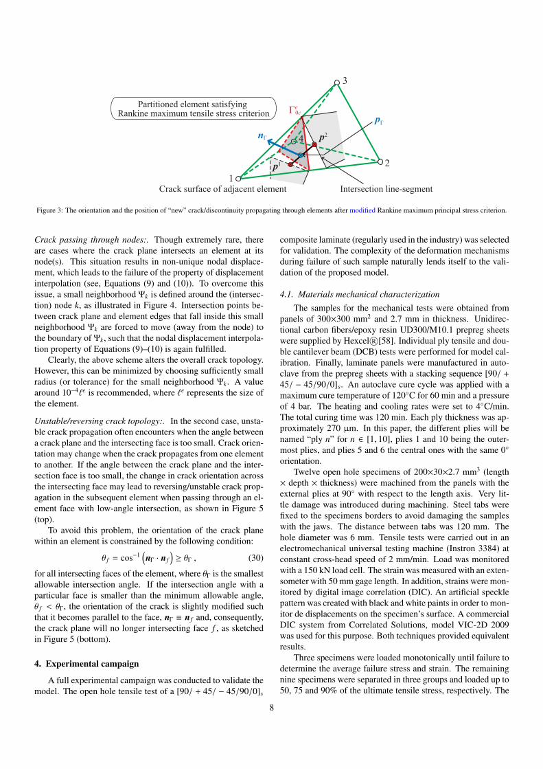
Once the crack orientation is defined, it needs to be at-tached, when applicable, to the cracks of the neighboring el-ements. Let pi be the mid-point of the intersection line-segmentbetween the element facet fi and the existing discontinuity planefrom the adjacent element, as illustrated in Figure 3. When themodified Rankine criterion is fulfilled, the crack surface/planeis formed within the element through a point pΓ, which is de-fined as

pΓ =1Ni

Ni∑i=1

pi , (28)

with Ni the total number of facets of the element that intersectwith the existing crack. This above condition is applied to en-sure the continuity of the crack path. Although in 3-dimensionalcases this condition cannot guarantee the connectivity of thepiecewise elementary crack planes across the element faces (seeFigure 3), the present scheme should be able to resemble the ap-proximation of the global crack surface [57]).

In case of crack initiation, where there is no existing crackpath adjacent elements, the crack position is assumed to formthrough the center of the element:

pΓ =1

Na

Na∑a=1

Xa , (29)

where Xa is the coordinate of the nodes, with Na the number ofnodes of the element.

3.3. Topological constraints for crack propagation

The present discrete/element-wise crack propagation modeloften encounters severe numerical instability issues. In the casespresented in this work, two crack propagation scenarii havebeen identified, which lead to unstable crack propagation.

7

Partitioned element satisfying Rankine maximum tensile stress criterion

12

3

4

Intersection line-segmentCrack surface of adjacent element

p2

p1

pΓ

Гe0c

nΓ

Figure 3: The orientation and the position of “new” crack/discontinuity propagating through elements after modified Rankine maximum principal stress criterion.

Crack passing through nodes:. Though extremely rare, thereare cases where the crack plane intersects an element at itsnode(s). This situation results in non-unique nodal displace-ment, which leads to the failure of the property of displacementinterpolation (see, Equations (9) and (10)). To overcome thisissue, a small neighborhood Ψk is defined around the (intersec-tion) node k, as illustrated in Figure 4. Intersection points be-tween crack plane and element edges that fall inside this smallneighborhood Ψk are forced to move (away from the node) tothe boundary of Ψk, such that the nodal displacement interpola-tion property of Equations (9)–(10) is again fulfilled.

Clearly, the above scheme alters the overall crack topology.However, this can be minimized by choosing sufficiently smallradius (or tolerance) for the small neighborhood Ψk. A valuearound 10−4`e is recommended, where `e represents the size ofthe element.

Unstable/reversing crack topology:. In the second case, unsta-ble crack propagation often encounters when the angle betweena crack plane and the intersecting face is too small. Crack orien-tation may change when the crack propagates from one elementto another. If the angle between the crack plane and the inter-section face is too small, the change in crack orientation acrossthe intersecting face may lead to reversing/unstable crack prop-agation in the subsequent element when passing through an el-ement face with low-angle intersection, as shown in Figure 5(top).

To avoid this problem, the orientation of the crack planewithin an element is constrained by the following condition:

θ f = cos−1(nΓ · nf

)≥ θΓ , (30)

for all intersecting faces of the element, where θΓ is the smallestallowable intersection angle. If the intersection angle with aparticular face is smaller than the minimum allowable angle,θ f < θΓ, the orientation of the crack is slightly modified suchthat it becomes parallel to the face, nΓ ≡ nf and, consequently,the crack plane will no longer intersecting face f , as sketchedin Figure 5 (bottom).

4. Experimental campaign

A full experimental campaign was conducted to validate themodel. The open hole tensile test of a [90/ + 45/ − 45/90/0]s

composite laminate (regularly used in the industry) was selectedfor validation. The complexity of the deformation mechanismsduring failure of such sample naturally lends itself to the vali-dation of the proposed model.

4.1. Materials mechanical characterization

The samples for the mechanical tests were obtained frompanels of 300×300 mm2 and 2.7 mm in thickness. Unidirec-tional carbon fibers/epoxy resin UD300/M10.1 prepreg sheetswere supplied by Hexcel R©[58]. Individual ply tensile and dou-ble cantilever beam (DCB) tests were performed for model cal-ibration. Finally, laminate panels were manufactured in auto-clave from the prepreg sheets with a stacking sequence [90/ +

45/ − 45/90/0]s. An autoclave cure cycle was applied with amaximum cure temperature of 120C for 60 min and a pressureof 4 bar. The heating and cooling rates were set to 4C/min.The total curing time was 120 min. Each ply thickness was ap-proximately 270 µm. In this paper, the different plies will benamed “ply n” for n ∈ [1, 10], plies 1 and 10 being the outer-most plies, and plies 5 and 6 the central ones with the same 0

orientation.Twelve open hole specimens of 200×30×2.7 mm3 (length

× depth × thickness) were machined from the panels with theexternal plies at 90 with respect to the length axis. Very lit-tle damage was introduced during machining. Steel tabs werefixed to the specimens borders to avoid damaging the sampleswith the jaws. The distance between tabs was 120 mm. Thehole diameter was 6 mm. Tensile tests were carried out in anelectromechanical universal testing machine (Instron 3384) atconstant cross-head speed of 2 mm/min. Load was monitoredwith a 150 kN load cell. The strain was measured with an exten-someter with 50 mm gage length. In addition, strains were mon-itored by digital image correlation (DIC). An artificial specklepattern was created with black and white paints in order to mon-itor de displacements on the specimen’s surface. A commercialDIC system from Correlated Solutions, model VIC-2D 2009was used for this purpose. Both techniques provided equivalentresults.

Three specimens were loaded monotonically until failure todetermine the average failure stress and strain. The remainingnine specimens were separated in three groups and loaded up to50, 75 and 90% of the ultimate tensile stress, respectively. The

8

12

3 =

4

Crack plane intersectingthe element at node 3

p2p1

Гe0c

12

3

4

Intersection pointmoved to theboundary of Ψ3

p2p1

Гe0c

p3

p3

Ψ3

Figure 4: Crack plane intersecting an element at one of its node: this intersection point is moved to the boundary of small neighborhood Ψk .

12

3

4

Small angle betweenthe crack plane and the intersecting face [234] p3

p2

p4

p1

nΓ

n[234]

12

3

4

p2

p3

p1nΓ = n[234]

Гe0c Гe

0c

Crack plane forcedparallel to face [234]

Γ0c

Modifiedcrack path

Γ0cIdeal projection

of crack path

Unstablecrack path

Unstable/reversing crack propagation indiscrete/element-wise crack topology

Figure 5: Unstable/reversing crack propagation due to change in crack orientation (top): orientation of the crack plane is modified to avoid unstable crack path(bottom).

tests were stopped at the set conditions and one specimen fromeach group was immersed in a dye penetrant liquid during 30minutes while holding the displacement constant. The dye pen-etrant procedure enhance the contrast between the cracks andthe composite material for tomographic measurements. The liq-uid was composed of 60 g of ZnI in 10 ml of water, 10 ml ofethanol and 10 ml of Kodak Photo-Flo 200. The specimen wasremoved from the machine and inspected by XCT as detailedbelow. It should be noticed that the stress-strain curve of all thespecimens were practically superposed.

4.2. X-ray Computed Tomography

The spatial distribution of the failure mechanisms was stud-ied by XCT using a Nanotom 160NF (GE Sensing & InspectionTechnologies Phoenix—X-ray). The tomograms were collectedat 100 kV and 120 µA using a tungsten target. For each tomo-gram, 2,000 radiographs were acquired with an exposure timeof 500 ms. Tomogram voxel size was set to 15 µm. The to-mograms were then reconstructed using an algorithm based onthe filtered back-projection procedure for Feldkamp cone beamgeometry. The damage in the reconstructed volumes was qual-itatively and quantitatively analyzed using the freeware ImageJ

9

software and the commercial software VGStudio Max 2.0. Ac-curate quantification of crack density and delaminated area waspossible because of the use of a dye penetrant liquid contain-ing ZnI which caused the cracks and delaminations to appearbrighter in the tomograms due to the higher X-ray absorptioncoefficient of ZnI as compared with the carbon fibers or thepolymeric matrix.

Damage at the interface between plies was evaluated fromseveral slices constituting that interface. The information ofdelaminated area was obtained from superimposed informationof these slices by projecting the maximum gray level (brightest)into one plane. The delaminated area was manually segmentedat each interface and for each loading condition.

The individuals plies at different orientations showed differ-ent cracking patterns. The cracks were properly detected thanksto the dye penetrant technique and were therefore, quantified ineach ply. Contrast fading between matrix and cracks occurswhen cracks with openings less than the tomographic resolu-tion are filled with the dye-penetrant. However, according toRef. [46], crack openings of about 5% of the reconstructedvoxel size can be detected using the dye penetrant technique.The selected intralaminar cracks were used to quantify matrixcrack density in each ply.

5. Results

In this section, the computational model is calibrated againstexperimental results and validated by direct quantitative com-parison between the experimental and simulated interlaminarand intralaminar failure. Finally, the scalability of the code isdemonstrated.

The stress-strain curves obtained from the open hole ten-sile test of the carbon fiber laminates are shown in Figure 6.The strain was determined using both the recording from theextensometer and the DIC data. The response was identical inboth cases. The average ultimate tensile stress determined fromthree samples was 479±17 MPa. The curves are quasi-linear upto the failure, although damage was already observed at 50%of the ultimate tensile stress (see damage analysis below). Thelinear behavior of the curves is mainly due to the 0 plies inwhich fiber fracture doesn’t occur until full sample failure. Thetests up to 50%, 75% and 90% of the ultimate stress are alsoincluded in Figure 6, confirming the high reproducibility of thetest.

The deformation maps obtained from the DIC measurementsat selected deformation conditions in the loading direction arepresented in Figure 7. The regions around the hole where thestrain ultimately localizes in the outer ply corresponds to the fi-nal fracture location, see Figures 7c and 7d. Similar strain local-ization patterns in open hole specimens have been observed pre-viously [59, 60], however in panels with different stacking se-quences than the one presented in this work. Note also that ad-ditional load introduction and alignment issues cannot be fullydiscarded. Although the DIC technique provides valuable infor-mation on the strain field (and fracture location in the externalply), it does not give information on the strain nor the damagemechanisms in the inner plies. Therefore, X-ray tomography

0 0.5 1 1.5·10−2

0

100

200

300

400

500

Strain

Stre

ss(M

Pa)

50% load75% load90% load

up to failuresimulation

Figure 6: Stress-strain curves for experimental tests and simulation.

was used below to investigate the damage mechanisms insidethe specimens.

5.1. Model calibration

The transversely isotropic mechanical properties correspond-ing to each ply of the laminate was obtained from single ply ten-sile tests. The values of the five elastic constants of the corre-sponding linear elastic transversely isotropic constitutive modelwere found to be El = 139.835 GPa, Et = 8.515 GPa, νl = 0.257,νt = 0.033 and Gl = 6.3 GPa (respectively, the longitudinal andtransversal Young’s moduli and Poisson’s ratios, and the shearmodulus).

The parameters of the two cohesive laws were also cali-brated from experiments. For the Rose–Ferrante law (interlam-inar intrinsic cohesive model), a DCB test was performed, ob-taining a fracture energy Gc = 600 N/m. Using this value, σc

was calibrated by simulating the DCB test. A value of σc = 60MPa provided the best fit for the force-displacement curve.

The parameters for the intralaminar extrinsic cohesive modelwere taken from previous work of the authors [31]. In this refer-ence, the calibration was done for the same material by use of amicro–meso-model of intra-laminar fracture which yielded Gc

= 121 N/m andσc = 45 MPa for the overall continuum intralam-inar failure, i.e., accounting for both matrix and matrix-fiberfailure). Figure 6 shows the numerical stress-strain curve ob-tained for the model parameters selected, truncated at the strainfor which the numerical sample fails, and confirms the validityof these parameters.

In order to compute the number of elements needed for themodel, the maximum cohesive element length α was estimatedfrom [16]:

α =π

8E Gc

σ2c (1 − ν2)

(31)

A good compromise for α for the interlaminar and intralaminarcohesive zones yielded a value of the order of tenths of microns,i.e. 4 million elements were needed for the mesh. Except for

10

(a) Deformation map at 0.2% strain (b) Deformation map at 0.8% strain

(c) Deformation map at 1.2% strain (d) Fractured specimen (at 1.3% strain)

Figure 7: Deformation maps for several strain conditions and fractured specimen after tensile test (surface with speckle pattern).

11

(a) Experimental sample in the initial state

(b) Numerical model used for the simulations

Figure 8: Initial states of experimental sample and numerical model beforetensile test.

(a) Experimental sample after the tensile test

(b) Numerical model after the simulation

Figure 9: Final states of experimental sample and numerical models after tensiletest.

the scalability study of Section 5.3, this mesh was used for thesubsequent results. Figures 8a and 8b show the initial states ofboth the experimental sample and the 4 million element numer-ical model after the tensile test.

Figures 9a and 9b show the states of both the experimentalsample and numerical model after the tensile test.

5.2. Quantitative damage analysis

Visual inspection of the volumes was performed after re-construction of the three 25%, 50% and 90% failure load sam-ples. The three specimens were scanned before loading to iden-tify any damage produced by machining. Very small edge de-lamination was observed around the hole and at the edges of thespecimens, and they were located between the two outermostplies (plies 1 and 2). The initial damage, probably introducedduring machining, was symmetrically distributed with respectto the loading axis. Despite the initial damage, the mechanicalresponse of the different specimens was identical and the dam-age developed during the tests was symmetrically distributedwith respect to the central ply (ply 5) as it will be shown later.

5.2.1. Matrix CrackingThe inspection of the tomographic data at 50% failure load

(0.6% strain) revealed that cracks appeared in all the plies ofthe specimens. In the outermost 90 plies (plies 1 and 9), ma-trix cracking was observed emanating from the border of thelaminate and growing towards the center of the laminate aboveand below the open hole region following the fiber direction.

On both sides of the hole the cracks were found to already en-compass the whole region between the hole and the edge. Inthe region above and below the hole, matrix cracking then de-veloped with deformation towards the center of the laminatein plies 1 and 9 until they either coalesced at the center of thelaminate or stopped growing when no crack grew from the op-posite direction at the same position, as it is observed in ply 1of Figure 10 for 90% failure load (1.1% strain).

In the +45 plies (plies 2 and 8) short matrix cracks (alsocalled “stitch cracks” to differentiate them from “developed cracks”)appeared over the positions of the 90 cracks. The density ofthe stitch cracks increased with deformation, see plies 2 and 8at 90% failure load in Figure 10. Most of the stitch cracks inthe +45 plies did not grow in length except for the ones locatedin a region at +45 (following the fibers direction) and contain-ing the hole, as well as some cracks located at the edges of thespecimen. The fact that the cracks maintained the same lengthbut increased in number is related to the susceptibility of crackgrowth to strain energy release rate and the crack spacing inthe adjacent and actual ply, as calculated for a [0/60/90]s and[0/30/90]s laminates in Refs. [61, 62].

Stitch cracks were not observed in the -45 plies (plies 3and 7), see Figure 10. Instead, developed cracks were observedas early as at 50% failure load, mainly around the hole at -45

following the fibers direction and in less proportion at the spec-imen’s edges. With further deformation, the cracks developedmainly in regions located at ±45 between the hole and at theedge of the specimens, however in these -45 plies the crackswere located predominantly at +45 from the hole, i.e. in a di-rection perpendicular to the fiber direction in these plies.

The 90 plies (plies 4 and 6), located between the -45 pliesand the central 0 ply, showed a slower development of thecracks with deformation when compared to the outer 90 plies.However, the crack density is noticeably higher (smaller crackspacing) than in the outer 90 plies, see Figure 10. Moreover, alarger concentration of cracks was noticed on both the right andleft sides of the hole in comparison with the regions above andbelow. Even at 90% failure load, most cracks above and belowthe hole did not encompass the whole laminate width and werearrested reaching a vertical imaginary line running tangentiallyto the hole in the loading direction. This effect is related to thedamage pattern in the central 0 ply (ply 5) in which two cracksgrew tangentially from right and left of the hole with deforma-tion following the loading direction, see Figure 10.

Finally, even if a complete quantitative analysis of the sim-ulations is provided below, it can already be noted that the sim-ulations qualitatively fit very closely the experimental results.

5.2.2. DelaminationFigure 11 show the interfaces between the outermost ply

and the central ply at 90% failure load. The images were ob-tained from superimposed information from the tomographicslices composing the interfaces stacked in the direction perpen-dicular to the plies. The delaminated area is displayed in Fig-ure 11 by the yellow envelopes delineating the damage.

Delamination between plies was first observed at 50% fail-ure load around the hole when cracks from subsequent plies

12

Experiment Simulation

ply

1(9

0)

ply

2(4

5)

ply

3(-

45 )

ply

4(9

0)

ply

5(0 )

Figure 10: Matrix cracks for plies 1,2,3,4 and 5 at 90% failure load.

13

(stitch and/or developed) intersected at the ply interface. Thedelaminated area around the hole increased with deformationand, at 75% failure load (0.9% strain), delamination at the edgesof the specimen was noticeable in the outermost interfaces. At90% failure load, delamination at the interface 1-2 (betweenplies 1 and 2), and its symmetric interface 8-9, progressed fromthe edges towards the interior of the laminate. This delamina-tion was located in the region confined between the 90 cracksand the stitch cracks in the +45 adjacent ply, see Figure 11.

The second interfaces (interfaces 2-3 and 6-7) showed at90% failure load the typical triangular shaped delamination en-closed between the ±45 cracks at the edges and around thehole, see Figure 11. Most of the delaminated area was locatedat +45 from the hole.

Towards the middle plane of the specimen (interfaces 3-4 and 4-5) delamination at the edges was less extensive thanaround the hole. Delamination developed mainly from crackintersection as shown in Figure 11 and was very well correlatedto the 0 ply cracks running parallel to the loading direction andtangentially to the open hole.

Again, the simulation results match very well the experi-mental results, despite a few differences at interplies 3-4 and4-5 underneath the hole, probably due to some experimentaldefects (by the lack of symmetry). It is also noticeable that theboundary effects on the delamination are remarkably well cap-tured.

5.2.3. Quantitative validationMatrix crack density was evaluated for each ply and for

the three measured deformation steps. The equivalent non-dimensional crack density was selected to quantify the crackdensity. It was obtained according to Ref. [53]:

ρeq =L tA

(32)

where L is the total crack length in every ply, t is the ply thick-ness (since all cracks encompass the whole ply thickness), andA is the in-plane area of the laminate measured by tomography.

The experimental non-dimensional crack density is presentedin Figure 12 and shows a very heterogeneous behavior for thedifferent plies. For instance, the outer and inner 90 plies (1and 9, and 4 and 6) showed different behaviors. While the out-ermost ply saturates after 75% failure load, the inner 90 pliescan withstand a higher crack density. The highest crack densitywas achieved in the inner 90 plies (plies 4 and 6) followed bythe density in the +45 plies (plies 2 and 8) where stitch crackspredominated. The high equivalent crack density observed inthe +45 plies (plies 2 and 8) suggests that the stitch cracksshould have a strong effect on the constraint ply stiffness. The-45 plies (plies 3 and 7) developed few cracks around the holeand the density in these plies only increased at the end of thetest. No stitch cracks were observed in these -45 plies. Thecrack density in the 0 ply (ply 5) is very low, as expected, andis a consequence of the development of the two cracks locatedtangentially to the hole, see Figure 12.

Figure 13 shows the non-dimensional crack density pro-vided by the simulation. It can be seen that experimental values

50 60 70 80 90

0

0.1

0.2

0.3

% of failure load

ρeq

ply 1ply 2ply 3ply 4ply 5

Figure 12: Experimental crack density.

50 60 70 80 90

0

5 · 10−2

0.1

0.15

0.2

0.25

0.3

% of failure load

ρeq

ply 1ply 2ply 3ply 4ply 5

Figure 13: Simulated crack density.

and simulation values are in very good agreement with eachother.The curve trend between experiments and simulations issimilar and the small differences between experiments and sim-ulations are within the experimental error.

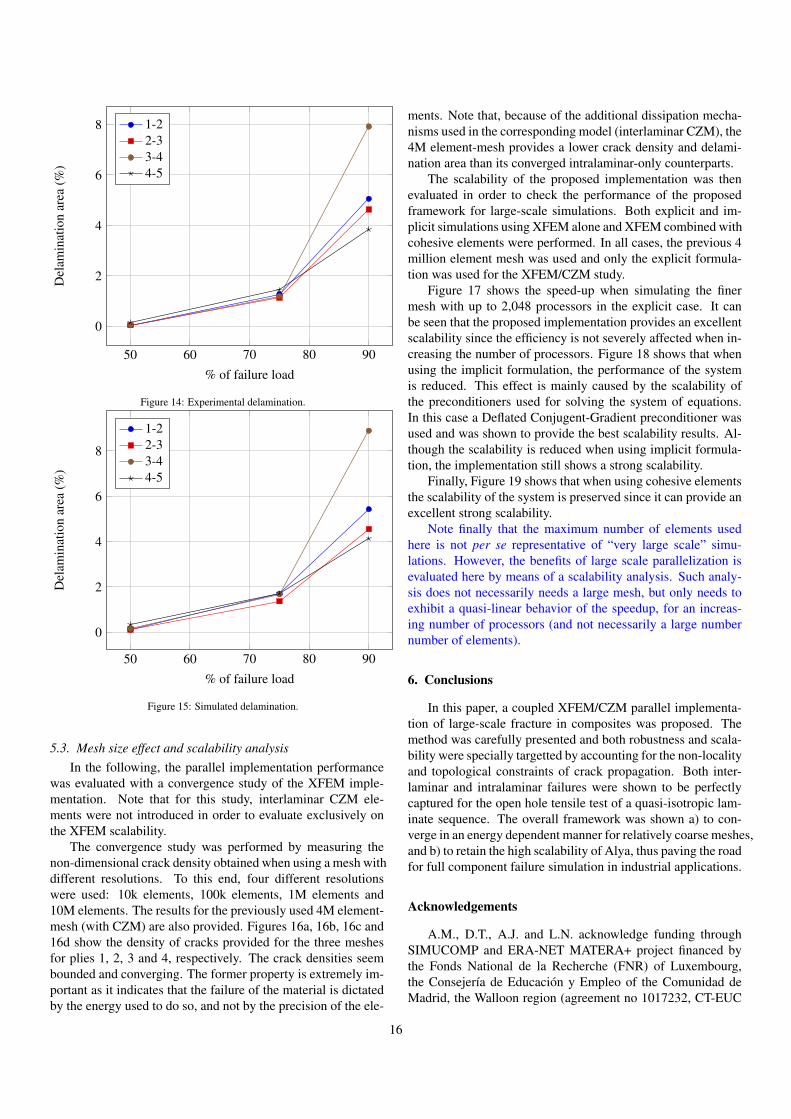
The delamination area obtained from the tomographic vol-umes is shown in Figure 14. The delaminated area was about0.1% at 50% failure load for all the plies. The development ofdelamination was symmetric with respect to the middle ply.

At 75% failure load, the delaminated area reached 1.2% andwas practically the same in all the plies. At 90% failure load,however, the delamination at the interfaces 3-4 and 6-7 devel-oped faster reaching 8.3%.

Figure 15 shows the area fraction of delamination obtainedfrom simulations, again providing an excellent comparison withthe experiments.

14

Experiment Simulation

inte

rply

1-2

inte

rply

2-3

inte

rply

3-4

inte

rply

4-5

Figure 11: Delamination at 90% failure load.

15

50 60 70 80 90

0

2

4

6

8

% of failure load

Del

amin

atio

nar

ea(%

)

1-22-33-44-5

Figure 14: Experimental delamination.

50 60 70 80 90

0

2

4

6

8

% of failure load

Del

amin

atio

nar

ea(%

)

1-22-33-44-5

Figure 15: Simulated delamination.

5.3. Mesh size effect and scalability analysisIn the following, the parallel implementation performance

was evaluated with a convergence study of the XFEM imple-mentation. Note that for this study, interlaminar CZM ele-ments were not introduced in order to evaluate exclusively onthe XFEM scalability.

The convergence study was performed by measuring thenon-dimensional crack density obtained when using a mesh withdifferent resolutions. To this end, four different resolutionswere used: 10k elements, 100k elements, 1M elements and10M elements. The results for the previously used 4M element-mesh (with CZM) are also provided. Figures 16a, 16b, 16c and16d show the density of cracks provided for the three meshesfor plies 1, 2, 3 and 4, respectively. The crack densities seembounded and converging. The former property is extremely im-portant as it indicates that the failure of the material is dictatedby the energy used to do so, and not by the precision of the ele-

ments. Note that, because of the additional dissipation mecha-nisms used in the corresponding model (interlaminar CZM), the4M element-mesh provides a lower crack density and delami-nation area than its converged intralaminar-only counterparts.

The scalability of the proposed implementation was thenevaluated in order to check the performance of the proposedframework for large-scale simulations. Both explicit and im-plicit simulations using XFEM alone and XFEM combined withcohesive elements were performed. In all cases, the previous 4million element mesh was used and only the explicit formula-tion was used for the XFEM/CZM study.

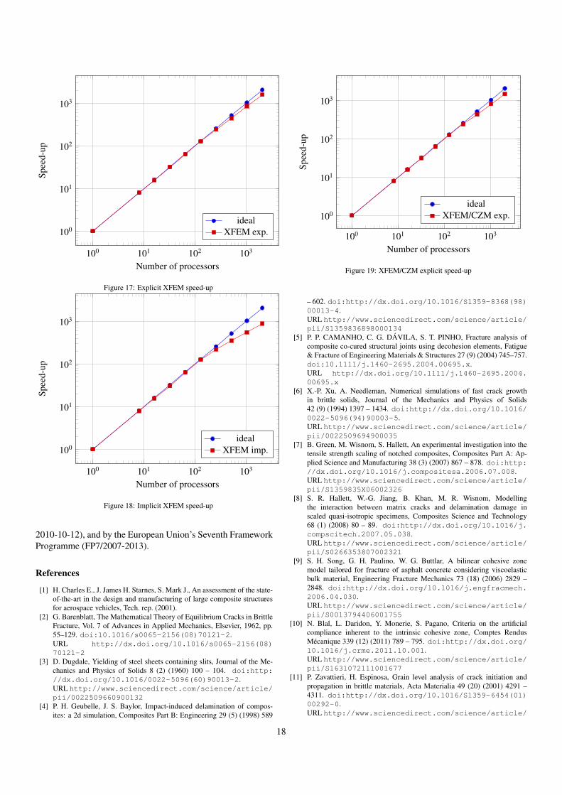
Figure 17 shows the speed-up when simulating the finermesh with up to 2,048 processors in the explicit case. It canbe seen that the proposed implementation provides an excellentscalability since the efficiency is not severely affected when in-creasing the number of processors. Figure 18 shows that whenusing the implicit formulation, the performance of the systemis reduced. This effect is mainly caused by the scalability ofthe preconditioners used for solving the system of equations.In this case a Deflated Conjugent-Gradient preconditioner wasused and was shown to provide the best scalability results. Al-though the scalability is reduced when using implicit formula-tion, the implementation still shows a strong scalability.

Finally, Figure 19 shows that when using cohesive elementsthe scalability of the system is preserved since it can provide anexcellent strong scalability.

Note finally that the maximum number of elements usedhere is not per se representative of “very large scale” simu-lations. However, the benefits of large scale parallelization isevaluated here by means of a scalability analysis. Such analy-sis does not necessarily needs a large mesh, but only needs toexhibit a quasi-linear behavior of the speedup, for an increas-ing number of processors (and not necessarily a large numbernumber of elements).

6. Conclusions

In this paper, a coupled XFEM/CZM parallel implementa-tion of large-scale fracture in composites was proposed. Themethod was carefully presented and both robustness and scala-bility were specially targetted by accounting for the non-localityand topological constraints of crack propagation. Both inter-laminar and intralaminar failures were shown to be perfectlycaptured for the open hole tensile test of a quasi-isotropic lam-inate sequence. The overall framework was shown a) to con-verge in an energy dependent manner for relatively coarse meshes,and b) to retain the high scalability of Alya, thus paving the roadfor full component failure simulation in industrial applications.

Acknowledgements

A.M., D.T., A.J. and L.N. acknowledge funding throughSIMUCOMP and ERA-NET MATERA+ project financed bythe Fonds National de la Recherche (FNR) of Luxembourg,the Consejerıa de Educacion y Empleo of the Comunidad deMadrid, the Walloon region (agreement no 1017232, CT-EUC

16

50 60 70 80 900

0.2

0.4

0.6

0.8

% of failure load

ρeq

10k100k1M10M

4M with CZM

(a) Ply 1 (90)

50 60 70 80 900

0.2

0.4

0.6

0.8

% of failure load

ρeq

10k100k1M10M

4M with CZM

(b) Ply 2 (+45)

50 60 70 80 900

0.2

0.4

0.6

0.8

% of failure load

ρeq

10k100k1M10M

4M with CZM

(c) Ply 3 (-45)

50 60 70 80 900

0.2

0.4

0.6

0.8

% of failure load

ρeq

10k100k1M10M

4M with CZM

(d) Ply 4 (90)

Figure 16: Convergence study.

17

100 101 102 103

100

101

102

103

Number of processors

Spee

d-up

idealXFEM exp.

Figure 17: Explicit XFEM speed-up

100 101 102 103

100

101

102

103

Number of processors

Spee

d-up

idealXFEM imp.

Figure 18: Implicit XFEM speed-up

2010-10-12), and by the European Union’s Seventh FrameworkProgramme (FP7/2007-2013).

References

[1] H. Charles E., J. James H. Starnes, S. Mark J., An assessment of the state-of-the-art in the design and manufacturing of large composite structuresfor aerospace vehicles, Tech. rep. (2001).

[2] G. Barenblatt, The Mathematical Theory of Equilibrium Cracks in BrittleFracture, Vol. 7 of Advances in Applied Mechanics, Elsevier, 1962, pp.55–129. doi:10.1016/s0065-2156(08)70121-2.URL http://dx.doi.org/10.1016/s0065-2156(08)70121-2

[3] D. Dugdale, Yielding of steel sheets containing slits, Journal of the Me-chanics and Physics of Solids 8 (2) (1960) 100 – 104. doi:http://dx.doi.org/10.1016/0022-5096(60)90013-2.URL http://www.sciencedirect.com/science/article/pii/0022509660900132

[4] P. H. Geubelle, J. S. Baylor, Impact-induced delamination of compos-ites: a 2d simulation, Composites Part B: Engineering 29 (5) (1998) 589

100 101 102 103

100

101

102

103

Number of processors

Spee

d-up

idealXFEM/CZM exp.

Figure 19: XFEM/CZM explicit speed-up

– 602. doi:http://dx.doi.org/10.1016/S1359-8368(98)00013-4.URL http://www.sciencedirect.com/science/article/pii/S1359836898000134

[5] P. P. CAMANHO, C. G. DAVILA, S. T. PINHO, Fracture analysis ofcomposite co-cured structural joints using decohesion elements, Fatigue& Fracture of Engineering Materials & Structures 27 (9) (2004) 745–757.doi:10.1111/j.1460-2695.2004.00695.x.URL http://dx.doi.org/10.1111/j.1460-2695.2004.00695.x

[6] X.-P. Xu, A. Needleman, Numerical simulations of fast crack growthin brittle solids, Journal of the Mechanics and Physics of Solids42 (9) (1994) 1397 – 1434. doi:http://dx.doi.org/10.1016/0022-5096(94)90003-5.URL http://www.sciencedirect.com/science/article/pii/0022509694900035

[7] B. Green, M. Wisnom, S. Hallett, An experimental investigation into thetensile strength scaling of notched composites, Composites Part A: Ap-plied Science and Manufacturing 38 (3) (2007) 867 – 878. doi:http://dx.doi.org/10.1016/j.compositesa.2006.07.008.URL http://www.sciencedirect.com/science/article/pii/S1359835X06002326

[8] S. R. Hallett, W.-G. Jiang, B. Khan, M. R. Wisnom, Modellingthe interaction between matrix cracks and delamination damage inscaled quasi-isotropic specimens, Composites Science and Technology68 (1) (2008) 80 – 89. doi:http://dx.doi.org/10.1016/j.compscitech.2007.05.038.URL http://www.sciencedirect.com/science/article/pii/S0266353807002321

[9] S. H. Song, G. H. Paulino, W. G. Buttlar, A bilinear cohesive zonemodel tailored for fracture of asphalt concrete considering viscoelasticbulk material, Engineering Fracture Mechanics 73 (18) (2006) 2829 –2848. doi:http://dx.doi.org/10.1016/j.engfracmech.2006.04.030.URL http://www.sciencedirect.com/science/article/pii/S0013794406001755

[10] N. Blal, L. Daridon, Y. Monerie, S. Pagano, Criteria on the artificialcompliance inherent to the intrinsic cohesive zone, Comptes RendusMecanique 339 (12) (2011) 789 – 795. doi:http://dx.doi.org/10.1016/j.crme.2011.10.001.URL http://www.sciencedirect.com/science/article/pii/S1631072111001677

[11] P. Zavattieri, H. Espinosa, Grain level analysis of crack initiation andpropagation in brittle materials, Acta Materialia 49 (20) (2001) 4291 –4311. doi:http://dx.doi.org/10.1016/S1359-6454(01)00292-0.URL http://www.sciencedirect.com/science/article/

18

pii/S1359645401002920[12] G. Camacho, M. Ortiz, Computational modelling of impact dam-

age in brittle materials, International Journal of Solids and Structures33 (20–22) (1996) 2899 – 2938. doi:http://dx.doi.org/10.1016/0020-7683(95)00255-3.URL http://www.sciencedirect.com/science/article/pii/0020768395002553

[13] M. Ortiz, A. Pandolfi, Finite-deformation irreversible cohesive elementsfor three-dimensional crack-propagation analysis, International Journalfor Numerical Methods in Engineering 44 (9) (1999) 1267–1282.doi:10.1002/(SICI)1097-0207(19990330)44:9<1267::AID-NME486>3.0.CO;2-7.URL http://dx.doi.org/10.1002/(SICI)1097-0207(19990330)44:9<1267::AID-NME486>3.0.CO;2-7

[14] A. Pandolfi, P. Guduru, M. Ortiz, A. Rosakis, Three dimensionalcohesive-element analysis and experiments of dynamic fracture inC300 steel, International Journal of Solids and Structures 37 (27)(2000) 3733 – 3760. doi:http://dx.doi.org/10.1016/S0020-7683(99)00155-9.URL http://www.sciencedirect.com/science/article/pii/S0020768399001559

[15] I. Arias, J. Knap, V. B. Chalivendra, S. Hong, M. Ortiz, A. J. Rosakis, Nu-merical modelling and experimental validation of dynamic fracture eventsalong weak planes, Computer Methods in Applied Mechanics and Engi-neering 196 (37–40) (2007) 3833 – 3840, ¡ce:title¿Special Issue Honor-ing the 80th Birthday of Professor Ivo Babuska¡/ce:title¿. doi:http://dx.doi.org/10.1016/j.cma.2006.10.052.URL http://www.sciencedirect.com/science/article/pii/S0045782507001107

[16] J. F. Molinari, G. Gazonas, R. Raghupathy, A. Rusinek, F. Zhou, Thecohesive element approach to dynamic fragmentation: the question ofenergy convergence, International Journal for Numerical Methods in En-gineering 69 (3) (2007) 484–503. doi:10.1002/nme.1777.URL http://dx.doi.org/10.1002/nme.1777

[17] A. Pandolfi, M. Ortiz, An efficient adaptive procedure for three-dimensional fragmentation simulations, Engineering with Computers18 (2) (2002) 148–159. doi:10.1007/s003660200013.URL http://dx.doi.org/10.1007/s003660200013

[18] A. Mota, J. Knap, M. Ortiz, Fracture and fragmentation of simplicial fi-nite element meshes using graphs, International Journal for NumericalMethods in Engineering 73 (11) (2008) 1547–1570. doi:10.1002/nme.2135.URL http://dx.doi.org/10.1002/nme.2135

[19] G. H. Paulino, W. Celes, R. Espinha, Z. J. Zhang, A general topology-based framework for adaptive insertion of cohesive elements in finite ele-ment meshes, Eng. with Comput. 24 (1) (2008) 59–78. doi:10.1007/s00366-007-0069-7.URL http://dx.doi.org/10.1007/s00366-007-0069-7

[20] V. K. Goyal, N. R. Jaunky, E. R. Johnson, D. R. Ambur, Intralaminarand interlaminar progressive failure analyses of composite panels withcircular cutouts, Composite Structures 64 (1) (2004) 91 – 105. doi:http://dx.doi.org/10.1016/S0263-8223(03)00217-4.URL http://www.sciencedirect.com/science/article/pii/S0263822303002174

[21] L. Daudeville, O. Allix, P. Ladeveze, Delamination analysis by damagemechanics: Some applications, Composites Engineering 5 (1) (1995) 17– 24. doi:http://dx.doi.org/10.1016/0961-9526(95)93976-3.URL http://www.sciencedirect.com/science/article/pii/0961952695939763

[22] P. Ladeveze, A damage computational approach for composites: Basicaspects and micromechanical relations, Computational Mechanics 17 (1-2) (1995) 142–150. doi:10.1007/BF00356486.URL http://dx.doi.org/10.1007/BF00356486

[23] J. Mergheim, E. Kuhl, P. Steinmann, A hybrid discontinuousgalerkin/interface method for the computational modelling of failure,Communications in Numerical Methods in Engineering 20 (7) (2004)511–519. doi:10.1002/cnm.689.URL http://dx.doi.org/10.1002/cnm.689

[24] R. Radovitzky, A. Seagraves, M. Tupek, L. Noels, A scalable 3d fracture

and fragmentation algorithm based on a hybrid, discontinuous galerkin,cohesive element method, Computer Methods in Applied Mechanics andEngineering 200 (1–4) (2011) 326 – 344. doi:http://dx.doi.org/10.1016/j.cma.2010.08.014.URL http://www.sciencedirect.com/science/article/pii/S0045782510002471

[25] M. Prechtel, G. Leugering, P. Steinmann, M. Stingl, Towards optimizationof crack resistance of composite materials by adjustment of fiber shapes,Engineering Fracture Mechanics 78 (6) (2011) 944 – 960. doi:http://dx.doi.org/10.1016/j.engfracmech.2011.01.007.URL http://www.sciencedirect.com/science/article/pii/S0013794411000117

[26] L. Noels, R. Radovitzky, A general discontinuous galerkin method forfinite hyperelasticity. formulation and numerical applications, Interna-tional Journal for Numerical Methods in Engineering 68 (1) (2006) 64–97. doi:10.1002/nme.1699.URL http://dx.doi.org/10.1002/nme.1699

[27] A. Ten Eyck, A. Lew, Discontinuous galerkin methods for non-linear elas-ticity, International Journal for Numerical Methods in Engineering 67 (9)(2006) 1204–1243. doi:10.1002/nme.1667.URL http://dx.doi.org/10.1002/nme.1667

[28] L. Noels, R. Radovitzky, An explicit discontinuous galerkin method fornon-linear solid dynamics: Formulation, parallel implementation andscalability properties, International Journal for Numerical Methods in En-gineering 74 (9) (2008) 1393–1420. doi:10.1002/nme.2213.URL http://dx.doi.org/10.1002/nme.2213

[29] A. Lew, A. Eyck, R. Rangarajan, Some applications of discontinuousgalerkin methods in solid mechanics, in: B. Reddy (Ed.), IUTAM Sympo-sium on Theoretical, Computational and Modelling Aspects of InelasticMedia, Vol. 11 of IUTAM BookSeries, Springer Netherlands, 2008, pp.227–236. doi:10.1007/978-1-4020-9090-5_21.URL http://dx.doi.org/10.1007/978-1-4020-9090-5_21

[30] A. T. Eyck, F. Celiker, A. Lew, Adaptive stabilization of discontinuousgalerkin methods for nonlinear elasticity: Motivation, formulation, andnumerical examples, Computer Methods in Applied Mechanics and En-gineering 197 (45–48) (2008) 3605 – 3622. doi:http://dx.doi.org/10.1016/j.cma.2008.02.020.URL http://www.sciencedirect.com/science/article/pii/S0045782508000789

[31] L. Wu, D. Tjahjanto, G. Becker, A. Makradi, A. Jerusalem, L. Noels,A micro–meso-model of intra-laminar fracture in fiber-reinforced com-posites based on a discontinuous Galerkin/cohesive zone method, Engi-neering Fracture Mechanics 104 (2013) 162–183. doi:10.1016/j.engfracmech.2013.03.018.

[32] G. Becker, L. Noels, A fracture framework for euler–bernoulli beamsbased on a full discontinuous galerkin formulation/extrinsic cohesive lawcombination, International Journal for Numerical Methods in Engineer-ing 85 (10) (2011) 1227–1251. doi:10.1002/nme.3008.URL http://dx.doi.org/10.1002/nme.3008

[33] G. Becker, C. Geuzaine, L. Noels, A one field full discontinuous galerkinmethod for kirchhoff–love shells applied to fracture mechanics, ComputerMethods in Applied Mechanics and Engineering 200 (45–46) (2011) 3223– 3241. doi:http://dx.doi.org/10.1016/j.cma.2011.07.008.URL http://www.sciencedirect.com/science/article/pii/S0045782511002490

[34] G. Becker, L. Noels, A full-discontinuous galerkin formulation of nonlin-ear kirchhoff–love shells: elasto-plastic finite deformations, parallel com-putation, and fracture applications, International Journal for NumericalMethods in Engineering 93 (1) (2013) 80–117. doi:10.1002/nme.4381.URL http://dx.doi.org/10.1002/nme.4381

[35] N. Moes, J. Dolbow, T. Belytschko, A finite element methodfor crack growth without remeshing, International Journal forNumerical Methods in Engineering 46 (1) (1999) 131–150.doi:10.1002/(SICI)1097-0207(19990910)46:1<131::AID-NME726>3.0.CO;2-J.URL http://dx.doi.org/10.1002/(SICI)1097-0207(19990910)46:1<131::AID-NME726>3.0.CO;2-J

19

[36] N. Moes, T. Belytschko, Extended finite element method for cohesivecrack growth, Engineering Fracture Mechanics 69 (7) (2002) 813 –833. doi:http://dx.doi.org/10.1016/S0013-7944(01)00128-X.URL http://www.sciencedirect.com/science/article/pii/S001379440100128X

[37] J. Dolbow, N. Moes, T. Belytschko, An extended finite element methodfor modeling crack growth with frictional contact, Computer Methodsin Applied Mechanics and Engineering 190 (51–52) (2001) 6825 –6846. doi:http://dx.doi.org/10.1016/S0045-7825(01)00260-2.URL http://www.sciencedirect.com/science/article/pii/S0045782501002602

[38] J. Melenk, I. Babuska, The partition of unity ynite element method: Ba-sic theory and applications. computer methods, Applied Mechanics andEngineering 39 (1996) 289–314.

[39] Alya system.URL http://www.bsc.es/computer-applications/alya-system

[40] E. Casoni, A. Jerusalem, C. Samaniego, B. Eguzkitza, P. Lafortune,D. Tjahjanto, X. Saez, G. Houzeaux, M. Vazquez, Alya: computationalsolid mechanics for supercomputers, Archives of Computational Methodsin Engineering.

[41] M. Vazquez, G. Houzeaux, R. Grima, J. Cela, Applications of parallelcomputational fluid mechanics in MareNostrum supercomputer: Low-mach compressible flows, in: PARCFD2007, Antalya (Turkey), 2007.

[42] G. Houzeaux, M. Vazquez, R. Aubry, J. Cela, A massively parallel frac-tional step solver for incompressible flows, JCP 228 (17) (2009) 6316–6332.

[43] G. Houzeaux, R. de la Cruz, H. Owen, M. Vazquez, Parallel uniformmesh multiplication applied to a navier-stokes solver, Computers & FluidsIn Press.

[44] B. Eguzkitza, G. Houzeaux, R. Aubry, H. Owen, M. Vazquez, A parallelcoupling strategy for the chimera and domain decomposition methods incomputational mechanics, Computers & Fluids.

[45] F. Sket, A. Enfedaque, C. Alton, C. Gonzalez, J. Molina-Aldareguia,J. Llorca, Automatic quantification of matrix cracking and fiber rota-tion by x-ray computed tomography in shear-deformed carbon fiber-reinforced laminates, Composites Science and Technology 90 (0)(2014) 129 – 138. doi:http://dx.doi.org/10.1016/j.compscitech.2013.10.022.URL http://www.sciencedirect.com/science/article/pii/S0266353813004223

[46] P. J. Schilling, B. R. Karedla, A. K. Tatiparthi, M. A. Verges, P. D. Her-rington, X-ray computed microtomography of internal damage in fiberreinforced polymer matrix composites, Composites Science and Technol-ogy 65 (14) (2005) 2071 – 2078. doi:http://dx.doi.org/10.1016/j.compscitech.2005.05.014.URL http://www.sciencedirect.com/science/article/pii/S0266353805001879

[47] K. Reifsnider, A. Talug, Analysis of fatigue damage in composite lami-nates, International Journal of Fatigue 2 (1) (1980) 3 – 11. doi:http://dx.doi.org/10.1016/0142-1123(80)90022-5.URL http://www.sciencedirect.com/science/article/pii/0142112380900225

[48] J. Masters, K. Reifsnider, An investigation of cumulative damage devel-opment in quasi-isotropic graphite/epoxy laminates., In: Reifsnider KL,editor. Damage in composite materials: mechanisms, accumulation, tol-erance, and characterization. ASTM STP 775 (1982) 40 – 62.

[49] J. Tong, F. Guild, S. Ogin, P. Smith, On matrix crack growth in quasi-isotropic laminates - i. experimental investigation, Composites Scienceand Technology 57 (11) (1997) 1527 – 1535. doi:http://dx.doi.org/10.1016/S0266-3538(97)00080-8.URL http://www.sciencedirect.com/science/article/pii/S0266353897000808

[50] W. Marsden, F. Guild, S. Ogin, P. Smith, Modelling stiffness–damage behaviour of (±45/90)s and (90/±45)s glass fibre re-inforced polymer laminates, Plastics, Rubber and Composites28 (1) (1999) 30–39. arXiv:http://www.maneyonline.com/doi/pdf/10.1179/146580199322913304, doi:10.1179/146580199322913304.

URL http://www.maneyonline.com/doi/abs/10.1179/146580199322913304

[51] L. Crocker, S. Ogin, P. Smith, P. Hill, Intra-laminar fracture in angle-ply laminates, Composites Part A: Applied Science and Manufacturing28 (9-10) (1997) 839 – 846. doi:http://dx.doi.org/10.1016/S1359-835X(97)00036-5.URL http://www.sciencedirect.com/science/article/pii/S1359835X97000365

[52] J. Varna, R. Joffe, N. Akshantala, R. Talreja, Damage in compos-ite laminates with off-axis plies, Composites Science and Technology59 (14) (1999) 2139 – 2147. doi:http://dx.doi.org/10.1016/S0266-3538(99)00070-6.URL http://www.sciencedirect.com/science/article/pii/S0266353899000706

[53] J. A. Lavoie, E. Adolfsson, Stitch cracks in constraint plies adjacent toa cracked ply, Journal of Composite Materials 35 (2001) 2077 – 2097.doi:10.1177/002199801772661362.URL http://jcm.sagepub.com/content/35/23/2077.abstract

[54] P. Johnson, F.-K. Chang, Characterization of matrix crack-induced lam-inate failure - part i: Experiments, Journal of Composite Materials35 (22) (2001) 2009 – 2035. doi:http://dx.doi.org/10.1106/7RN1-PFBN-XQR9-3KDK.URL http://jcm.sagepub.com/content/35/22/2009

[55] M. S., Extended Finite Element Method for Fracture Analysis of Struc-tures, Blackwell Publishing Ltd., 2008.

[56] F. Van Der Meer, L. Sluys, Continuum models for the analysis of pro-gressive failure in composite laminates, Journal of Composite Materials43 (20) (2009) 2131–2155. doi:10.1177/0021998309343054.

[57] T. Gasser, G. Hozapfel, Modeling 3d crack propagation in unreinforcedconcrete using pufem, Computer Methods in Applied Mechanics and En-gineering 194 (2005) 2859–2896.

[58] Hexcel corporation.URL http://www.hexcel.com

[59] F. Pierron, B. Green, M. Wisnom, S. Hallett, Full-field assessment of thedamage process of laminated composite open-hole tensile specimens. PartII: Experimental results, Composites: Part A 38 (2007) 2321–2332. doi:10.1016/j.compositesa.2007.01.019.

[60] M. Caminero, M. Lopez-Pedrosa, C. Pinna, C. Soutis, Damage monitor-ing and analysis of composite laminates with an open hole and adhesivelybonded repairs using digital image correlation, Composites: Part B 53(2013) 76–91. doi:10.1016/j.compositesb.2013.04.050.

[61] T. Yokozeki, T. Aoki, T. Ogasawara, T. Ishikawa, Effects of layup angleand ply thickness on matrix crack interaction in contiguous plies of com-posite laminates, Composites Part A: Applied Science and Manufacturing36 (9) (2005) 1229 – 1235. doi:http://dx.doi.org/10.1016/j.compositesa.2005.02.002.URL http://www.sciencedirect.com/science/article/pii/S1359835X05000692

[62] J. Xu, B. V. Sankar, Prediction of stitch crack evolution and gaspermeability in multidirectional composite laminates, Composites PartA: Applied Science and Manufacturing 39 (10) (2008) 1625 –1631. doi:http://dx.doi.org/10.1016/j.compositesa.2008.07.003.URL http://www.sciencedirect.com/science/article/pii/S1359835X08001887

20