ORIGINAL PAPER - PRODUCTION ENGINEERING

An investigation on economy and CO2 emission of wateralternating steam process (WASP) using response surfacecorrelation

A. M. Suranto1 • A. K. Permadi2 • W. Bae3

Received: 19 January 2016 / Accepted: 13 November 2016 / Published online: 23 December 2016

� The Author(s) 2016. This article is published with open access at Springerlink.com

Abstract In steamflooding, the steam tends to move

toward the upper portion of the reservoir due to the grav-

itational effect causing poor drainage in the lower sec-

tion. This causes the steam to breakthrough to the

production well early. The water alternating steam process

(WASP) often provides a solution to the problem. How-

ever, studies on WASP are found very limited despite the

fact that this process is sensitive to the operating condi-

tions. By investigating the WASP using response surface

correlation, the factors governing steam injections opera-

tions are evaluated. To achieve the maximum net present

value (NPV), several operating conditions are investigated.

The side effect of gas fuel burning in the steam generation,

i.e., CO2 emission, is considered in selecting the optimum

operating condition. As illustrated by reservoir simulation

results, if the economy is prioritized and oil price is 45 $/

barrel, the optimum case is achieved in which the WASP-

start is 3.0 years, the WASP-cycle is 3.5 months, and the

steam/water injection rate is 141 m3/day. The resulting

NPV is 14.1 MM$, and the CO2 emission is

28.53 9 103 tonnes.

Keywords Steamflooding � Water alternating steam

process � Heavy oil � Net present value � CO2 emission �Response surface correlation

List of symbols

WASP Water alternating steam process

NPV Net present value

NCF Net cash flow

I Discount rate

N Project’s economic life in years

GJ Giga Joule

$ United State Dollars

SI metric conversion factors

Lb 0.454 kg

�F (�C 9 9/5) ? 32

bbl 9 1.5899 m3

cp 9 1.0 Pa.s

tonne 1000 kg

psi 6.895 kPa

Introduction

Steamflooding is a process in which steam is injected into

the reservoir that it transfers its heat to the rock and fluids.

Generally, there are four separated zones in a steamflood-

ing process namely (1) oil bank, (2) hot water bank, (3)

solvent bank, and (4) steam zone (Hong 1994). This pro-

cess occurs while the oil bank moves toward the production

well. After the pore is saturated with steam, the steam tends

to move to the top of the reservoir since it is lighter than

& A. M. Suranto

su_ranto@upnyk.ac.id

A. K. Permadi

akp@tm.itb.ac.id

W. Bae

wsbae@sejong.ac.kr

1 Department of Petroleum Engineering, Universitas

Pembangunan Nasional ‘‘Veteran’’ Yogyakarta, Jalan Ring

Road Utara, Condong Catur, Yogyakarta 55283, Indonesia

2 Department of Petroleum Engineering, Bandung Institute of

Technology, Jalan Ganesa No. 10, Bandung 40132, Indonesia

3 Department of Energy and Mineral Resources Engineering,

Sejong University, 98 Gunja-dong, Gwangjin-gu, Seoul

143-747, South Korea

123

J Petrol Explor Prod Technol (2017) 7:1125–1132

DOI 10.1007/s13202-016-0307-x

reservoir fluids. Therefore, in a continuous injection pro-

cess, the steam will breakthrough early to the production

well. Even though the steam injection rate remains con-

stant, the oil production rate decreases while the steam oil

ratio (SOR) increases. Because the steam is produced by

way of burning natural gases, in such a process the CO2

emission per produced-oil volume also increases.

In order to avoid early steam breakthrough, the first

approach was steamflooding followed by hot water-

flooding, which was successfully applied in the Kern

River field. It was found that the production increased

after the hot water had been injected. The main reason for

such a strategy is that it would prevent a significant loss

in production rate. It might also improve the sweep effi-

ciency and prevents the migration of the left-behind oil

into the portions of the reservoir which had been swept by

the steam (Ault et al. 1985). The further approach was

water alternating steam process (WASP). Section 13D of

West Coalinga Field was the first WASP pilot project.

They claimed that WASP eliminated early steam break-

through and channeling problems, reduced fuel con-

sumption for steam generation and improved incremental

oil sale (Hong and Stevens 1990). A successful WASP

has also been reported in some other fields such as North

Palo Seco, Apex Quarry, Central Las Bajo, and Bennett

Village (Ramlal and Singh 2001).

Although most of WASP projects have been applied

successfully, studies on WASP have rarely been reported

in the literature. To fill this gap, this paper proposes a

‘‘response surface correlation’’ generated by an experi-

mental design and response surface methodology to

investigate the economy and CO2 emission problems. In

this method, the operating conditions are varied to

achieve the maximum NPV, the side effect CO2 emission

is calculated, and the most sensitive operating conditions

are identified.

Methodology overview

Response surface methodology is a collection of mathe-

matical and statistical techniques that is useful for model-

ing and analyzing problems. In this method, the

relationships between response and unknown-independent

variables are established (Douglas 2001). If the problem is

simple enough, then the response might be well modeled

by a linear function. Furthermore, if the problem is more

complicated, the equation may be described by second

order as follows:

y ¼ b0 þ b1x1 þ b2x2 þ b3x21 þ b4x

22 þ � � � þ bkx

nk þ C

ð1Þ

where bk are constant coefficients, x is the independent

variable, k is the factor coefficient, n is the order of

equation, and

”

is an error. In order to estimate the

response, the ANOVA method is applied. There are several

functions which can used to approximate the response such

as first-order, second-order, or third-order functions

depending on the complexity of variable relationships. To

understand the response, one needs to do the experiment

design. The foundational principle of this is to select a set

of variable combinations from a number of scenarios while

it is still adequate to build the relationship among the

independent variables and the response at a certain confi-

dence level.

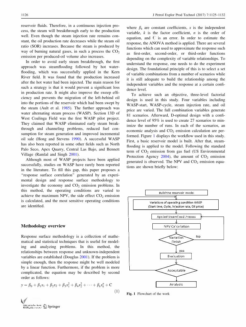
To achieve such an objective, three-level factorial

design is used in this study. Four variables including

WASP-start, WASP-cycle, steam injection rate, and oil

price are varied. The full combination variables generate

81 scenarios. Afterward, D-optimal design with a confi-

dence level of 95% is used to create 27 scenarios to min-

imize the number of runs. In each of the scenarios, an

economic analysis and CO2 emission calculation are per-

formed. Figure 1 displays the workflow used in this study.

First, a basic reservoir model is built. After that, steam-

flooding is applied to the model. Following the standard

term of CO2 emission from gas fuel (US Environmental

Protection Agency 2004), the amount of CO2 emission

generated is observed. The NPV and CO2 emission equa-

tions are shown briefly below:

Fig. 1 Flowchart of the work

1126 J Petrol Explor Prod Technol (2017) 7:1125–1132

123

NPV ¼XN

t¼0

NCFt

1þ ið Þtð2Þ

CO2 emission kgð Þ ¼ 50� heat employed GJð Þ ð3Þ

The next step is evaluating the outcomes of each

scenario. If the optimum condition cannot be found in this

area of design space, the search is continued in another area

following a steepest-ascent direction.

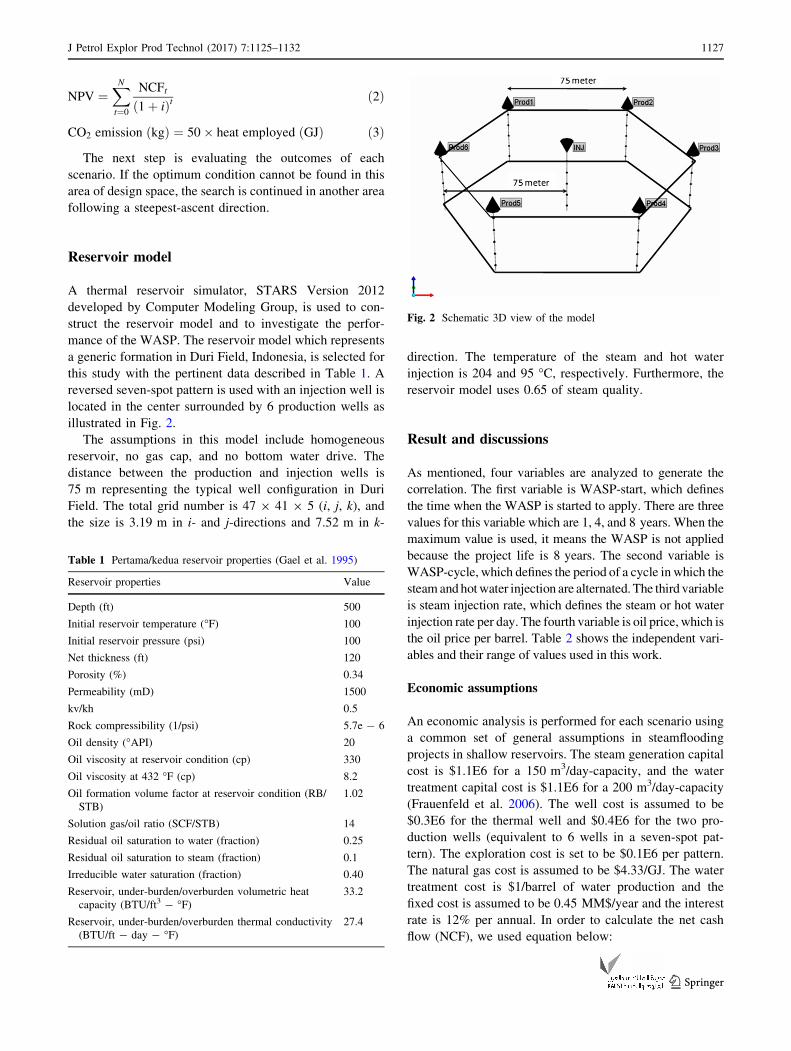
Reservoir model

A thermal reservoir simulator, STARS Version 2012

developed by Computer Modeling Group, is used to con-

struct the reservoir model and to investigate the perfor-

mance of the WASP. The reservoir model which represents

a generic formation in Duri Field, Indonesia, is selected for

this study with the pertinent data described in Table 1. A

reversed seven-spot pattern is used with an injection well is

located in the center surrounded by 6 production wells as

illustrated in Fig. 2.

The assumptions in this model include homogeneous

reservoir, no gas cap, and no bottom water drive. The

distance between the production and injection wells is

75 m representing the typical well configuration in Duri

Field. The total grid number is 47 9 41 9 5 (i, j, k), and

the size is 3.19 m in i- and j-directions and 7.52 m in k-

direction. The temperature of the steam and hot water

injection is 204 and 95 �C, respectively. Furthermore, the

reservoir model uses 0.65 of steam quality.

Result and discussions

As mentioned, four variables are analyzed to generate the

correlation. The first variable is WASP-start, which defines

the time when the WASP is started to apply. There are three

values for this variable which are 1, 4, and 8 years. When the

maximum value is used, it means the WASP is not applied

because the project life is 8 years. The second variable is

WASP-cycle, which defines the period of a cycle in which the

steamandhotwater injection are alternated. The third variable

is steam injection rate, which defines the steam or hot water

injection rate per day. The fourth variable is oil price, which is

the oil price per barrel. Table 2 shows the independent vari-

ables and their range of values used in this work.

Economic assumptions

An economic analysis is performed for each scenario using

a common set of general assumptions in steamflooding

projects in shallow reservoirs. The steam generation capital

cost is $1.1E6 for a 150 m3/day-capacity, and the water

treatment capital cost is $1.1E6 for a 200 m3/day-capacity

(Frauenfeld et al. 2006). The well cost is assumed to be

$0.3E6 for the thermal well and $0.4E6 for the two pro-

duction wells (equivalent to 6 wells in a seven-spot pat-

tern). The exploration cost is set to be $0.1E6 per pattern.

The natural gas cost is assumed to be $4.33/GJ. The water

treatment cost is $1/barrel of water production and the

fixed cost is assumed to be 0.45 MM$/year and the interest

rate is 12% per annual. In order to calculate the net cash

flow (NCF), we used equation below:

Table 1 Pertama/kedua reservoir properties (Gael et al. 1995)

Reservoir properties Value

Depth (ft) 500

Initial reservoir temperature (�F) 100

Initial reservoir pressure (psi) 100

Net thickness (ft) 120

Porosity (%) 0.34

Permeability (mD) 1500

kv/kh 0.5

Rock compressibility (1/psi) 5.7e - 6

Oil density (�API) 20

Oil viscosity at reservoir condition (cp) 330

Oil viscosity at 432 �F (cp) 8.2

Oil formation volume factor at reservoir condition (RB/

STB)

1.02

Solution gas/oil ratio (SCF/STB) 14

Residual oil saturation to water (fraction) 0.25

Residual oil saturation to steam (fraction) 0.1

Irreducible water saturation (fraction) 0.40

Reservoir, under-burden/overburden volumetric heat

capacity (BTU/ft3 - �F)33.2

Reservoir, under-burden/overburden thermal conductivity

(BTU/ft - day - �F)27.4

Fig. 2 Schematic 3D view of the model

J Petrol Explor Prod Technol (2017) 7:1125–1132 1127

123

NCF ¼ Gross revenue½ �� Well cost thermal wellþ Non thermal wellð½þExploration costÞ� � Steam generation cost½ �� Water treatment cost½ � � Natural gas cost½ �� Fixed cost½ �

ð4Þ

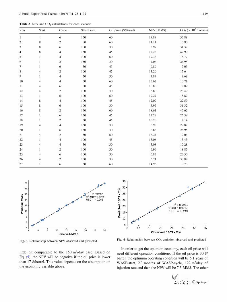
By using standard term on CO2 and economy above,

Table 3 displays the NPV and CO2 emission calculation

results. To calculate the NPV, Eqs. (2) and (4) have been

employed. The gross revenue is function of oil production

rate as result from reservoir simulation. The CO2 emission

is calculated by Eq. (3). The heat employed is also

calculated by reservoir simulation.

Fitted model

The relationship between the independent variables and the

response is constructed using the quadratic model. By

using this model, the relationship between the independent

variables and the response can be described as:

NPV MM$ð Þ ¼ �12:0871þ 0:375491 Að Þ þ 0:505609 Bð Þþ 0:092169 Cð Þ þ 0:38321 Dð Þ� 0:0547919 A2

� �þ 0:0322998 ABð Þ

� 0:00136669 ACð Þ � 0:00158124 ADð Þ� 0:0386117 B2

� �� 0:00101391 BCð Þ

� 0:00560595 BDð Þ � 0:000460315 C2� �

þ 0:000932527 CDð Þ � 0:000453058 D2� �

ð5Þ

CO2 �103 tonnes� �

¼ 3:26189� 1:04622 Að Þ� 1:93923 Bð Þ þ 0:216004 Cð Þþ 0:112553 A2

� �

� 0:00933755 ABð Þþ 0:0185834 ACð Þ þ 0:236503 B2

� �

þ 0:00052458 BCð Þ� 0:000361654 C2

� �

ð6Þ

where A is WASP-start (year), B is WASP-cycle (month),

C is steam/water injection rate (m3/day), and D is oil price

per barrel. To validate the equation, Figs. 3 and 4 showing

the plot between the observed and the predicted NPV and

CO2 emission, respectively, are evaluated. The predicted

parameters are calculated using Eqs. (5) and (6). The

determination coefficient (R2) and the adjusted determina-

tion coefficient (R2 Adj) are close to one exhibiting the

model is adequate. The low value of the residual standard

deviation (RSD) indicates the accuracy of the relationship.

Interaction effects

The interaction effects between the independent variables

and the response are shown in Figs. 5 and 6. These effects

are calculated from the polynomial model described by

Eqs. (5) and (6). The Pareto graph consists of two groups.

One group of factor coefficients is positive meaning that if

the values of these factors increase, then the NPV and CO2

emission also increase. The other group is negative

meaning that increasing the value of the factors will cause

the response to decrease.

In the economic analysis, two parameters have positive

effects on the NPV. These are steam injection rate and oil

price. The effect of oil price is larger than the steam

injection rate. On the other hand, the parameters that have

negative effects are WASP-start and WASP-cycle. How-

ever, the WASP-start has a little effect on the NPV.

In the CO2 emission part, the oil price does not include

in the calculation since it will be not affected by the CO2

emission. There are two parameters that have positive

effect. These are WASP-start and steam injection rate. The

effect of injection rate is the higher compared to WASP-

start. The WASP-cycle has a little negative effect on the

CO2 emission. As a result, increasing the WASP-start and

steam injection rate will increase the CO2 emission.

Proposed response surface correlation for economy

and CO2 emission

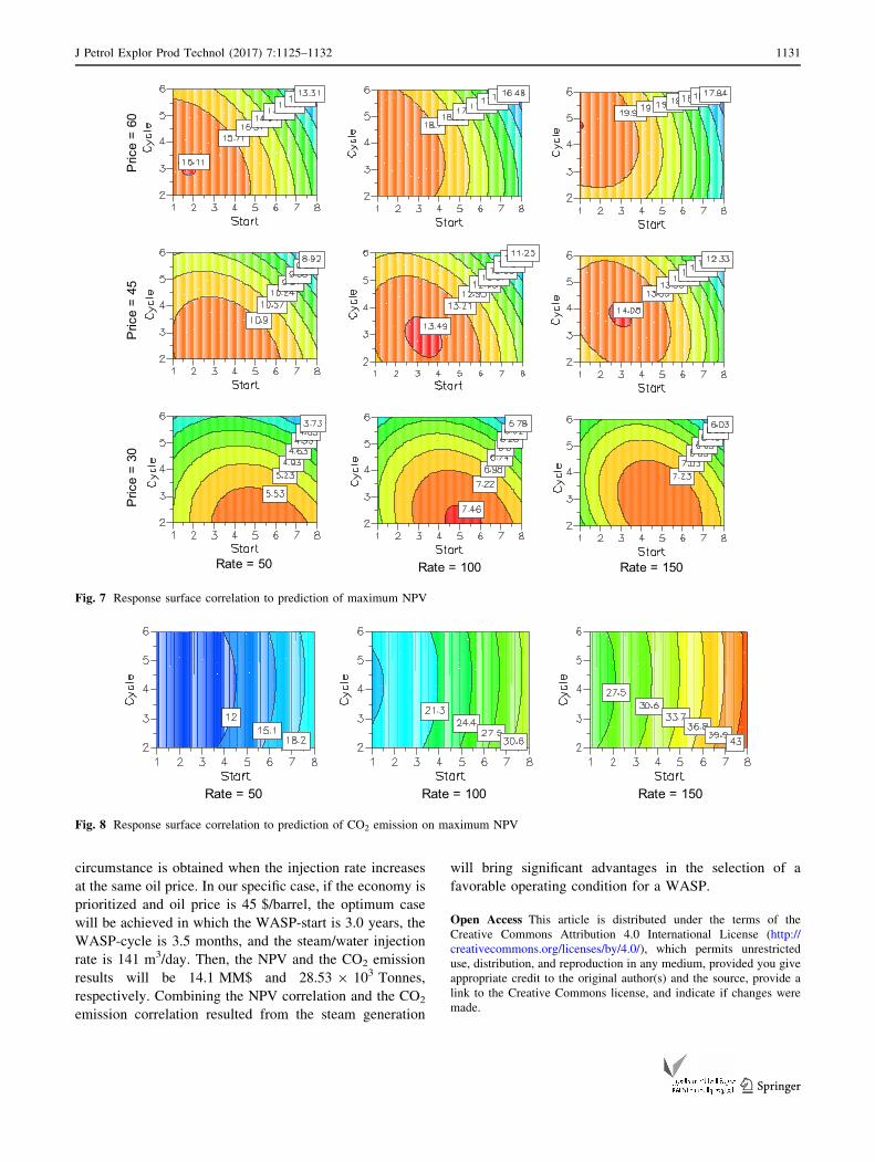
Figure 7 displays the surface correlation for the economic

analysis. At the same steam injection rate, if the oil price

increases, the NPV will dramatically increase. For exam-

ple, at the injection rate of 50 m3/day, if the oil price

increases from 30 to 60 $/barrel, the NPV will increase

from 5.53 to 16.11 MM$. The degree of the increment is

analogous to the injection rate of 100 m3/day case and a

Table 2 Range of parameters for this research

Parameter Minimum Middle Maximum

WASP-start (year) 1 4 8

WASP-cycle (month) 2 4 6

Steam injection rate (m3/day) 50 100 150

Oil price (US$/barrel) 30 45 60

1128 J Petrol Explor Prod Technol (2017) 7:1125–1132

123

little bit comparable to the 150 m3/day case. Based on

Eq. (5), the NPV will be negative if the oil price is lower

than 17 $/barrel. This value depends on the assumption on

the economic variable above.

In order to get the optimum economy, each oil price will

need different operation conditions. If the oil price is 30 $/

barrel, the optimum operating condition will be 5.1 years of

WASP-start, 2.3 months of WASP-cycle, 122 m3/day of

injection rate and then the NPV will be 7.3 MM$. The other

Table 3 NPV and CO2 calculations for each scenario

Run Start Cycle Steam rate Oil price ($/Barrel) NPV (MM$) CO2 (9 103 Tonnes)

1 4 6 150 60 19.89 33.88

2 8 2 50 60 14.14 15.90

3 8 6 100 30 5.97 31.32

4 8 4 150 45 12.23 42.99

5 1 4 100 60 19.33 18.77

6 1 2 150 30 7.06 26.95

7 1 6 50 45 9.89 7.05

8 4 2 100 45 13.20 17.6

9 1 4 50 30 4.84 9.68

10 4 4 50 60 15.62 10.71

11 4 6 50 45 10.80 8.89

12 4 2 100 30 6.80 23.49

13 1 6 100 60 19.27 18.87

14 8 4 100 45 12.09 22.59

15 8 6 100 30 5.97 31.32

16 8 2 150 60 18.61 45.62

17 1 6 150 45 13.29 25.59

18 1 2 50 45 10.20 7.14

19 4 4 150 30 6.98 29.87

20 1 6 150 30 6.83 26.95

21 4 2 50 60 16.24 12.04

22 1 4 100 45 13.06 13.43

23 4 4 50 30 5.08 10.28

24 1 2 100 30 6.96 18.85

25 4 6 100 30 6.87 23.50

26 4 2 150 30 6.71 33.88

27 1 6 50 60 14.96 9.73

Fig. 3 Relationship between NPV observed and predicted Fig. 4 Relationship between CO2 emission observed and predicted

J Petrol Explor Prod Technol (2017) 7:1125–1132 1129

123

condition, if the oil price is 45 $/barrel, the optimum oper-

ating condition will be 3 years of WASP-start, 3.5 months

of WASP-cycle, 141 m3/day of injection rate and then the

NPV will be 14.1 MM$. While, if the oil price is 60 $/day,

the optimum operating condition will be 1.1 years of

WASP, 4.7 months of WASP-cycle, 149 m3/day of injec-

tion rate and then the NPV will be 20.54 MM$. Increasing

the oil price at the same steam injection rate will decline the

WASP-start and raise the WASP-cycle.

Figure 8 shows the surface correlation between the

WASP operating condition and the side effect CO2 emis-

sion. In the low steam injection rate case, the CO2 emission

is more favorable. At this condition, WASP-cycle has not

an effect on the CO2 emission. In the contrary, at the

WASP-start and steam injection rate have a significant

effect on the CO2 emission. The increasing of WASP-start

also tends to increase the CO2 emissions for all cases of the

steam injection rate. This phenomenon is quite different

compared to that observed in the economic analysis part.

The CO2 emission is only a function of heat consumption

while the NPV is related to the oil production, oil price, and

economic assumptions.

Finally, the CO2 emission based on the above optimum

operating conditions for each the oil price shows if the oil

price is 30, 45, and 60 $/barrel, the CO2 emission will be

approximately 30.21 9 103, 28.53 9 103, and

25.88 9 103 Tonnes, respectively. In the optimum case,

increasing oil price will influence to decrease CO2 emis-

sion. Hence, by using surface correlations for the NPV and

CO2 emission, the operating condition can be set up to

select which one is more favorable.

Conclusions

This study demonstrates the water alternating steam pro-

cess (WASP) that can be economically optimized by

applying a response surface correlation. Four parameters

used are WASP-start, WASP-cycle, steam/water injection

rate, and oil price. The oil price significantly influences to

the NPV, while the WASP-start does not have significant

effects on the NPV. In the maximum NPV case, increasing

oil price at the same steam injection rate reduces the

WASP-start and raises the WASP-cycle. Similar

-1

0

1

2

3

4

5

Sta

Cyc Rat Pri

Sta

*Sta

Cyc

*Cyc

Rat

*Rat

Pri*

Pri

Sta

*Cyc

Sta

*Rat

Sta

*Pri

Cyc

*Rat

Cyc

*Pri

Rat

*Pri

MM

US

$

Fig. 5 Pareto chart for selecting response to NPV

0

2

4

6

8

Sta

Cyc Rat

Sta

*Sta

Cyc

*Cyc

Rat

*Rat

Sta

*Cyc

Sta

*Rat

Cyc

*Rat

10^3

x T

on

Fig. 6 Pareto chart for selecting response to CO2 emission

1130 J Petrol Explor Prod Technol (2017) 7:1125–1132

123

circumstance is obtained when the injection rate increases

at the same oil price. In our specific case, if the economy is

prioritized and oil price is 45 $/barrel, the optimum case

will be achieved in which the WASP-start is 3.0 years, the

WASP-cycle is 3.5 months, and the steam/water injection

rate is 141 m3/day. Then, the NPV and the CO2 emission

results will be 14.1 MM$ and 28.53 9 103 Tonnes,

respectively. Combining the NPV correlation and the CO2

emission correlation resulted from the steam generation

will bring significant advantages in the selection of a

favorable operating condition for a WASP.

Open Access This article is distributed under the terms of the

Creative Commons Attribution 4.0 International License (http://

creativecommons.org/licenses/by/4.0/), which permits unrestricted

use, distribution, and reproduction in any medium, provided you give

appropriate credit to the original author(s) and the source, provide a

link to the Creative Commons license, and indicate if changes were

made.

Rate = 50

06=

ecirP

54=

ecirP

0 3=

e cirP

Rate = 100 Rate = 150

Fig. 7 Response surface correlation to prediction of maximum NPV

Rate = 50 Rate = 100 Rate = 150

Fig. 8 Response surface correlation to prediction of CO2 emission on maximum NPV

J Petrol Explor Prod Technol (2017) 7:1125–1132 1131

123

References

Ault JW, Johnson WM, Kamilos GN (1985) Conversion of mature

steamfloods to low-quality steam and/or hot-water injection

projects. Soc Pet Eng. doi:10.2118/13604-MS

Douglas CM (2001) Design and analysis of experiments. Douglas C.

Montgomery, 5th edn. Arizona State University, Wiley, New

York

Frauenfeld TW, Deng X, Jossy C (2006) Economic analysis of

thermal solvent processes. Pet Soc Can. doi:10.2118/2006-164

Gael BT, Gross SJ, McNaboe GJ (1995) Development planning and

reservoir management in the Duri steam flood. Soc Pet Eng.

doi:10.2118/29668-MS

Hong KC (1994) Steamflood reservoir management: thermal enhance

oil recovery. Pennwell Publishing Company, Tulsa

Hong KC, Stevens DE (1990) Water-alternating-steam process

improves project economics at West Coalinga field. Pet Soc

Can. doi:10.2118/90-84

Ramlal V, Singh KS (2001) Success of water-alternating-steam-

process for heavy oil recovery. Soc Pet Eng. doi:10.2118/69905-

MS

US Environmental Protection Agency (2004) Unit conversions,

emissions factors, and other reference data, United States

Environmental Protection Agency. http://www.epa.gov/cpd/pdf/

brochure.pdf

1132 J Petrol Explor Prod Technol (2017) 7:1125–1132

123