an investigation into the pattern of delayed marriage … 275 - baishali_delayed marriage 15...
TRANSCRIPT

An Investigation into thePattern of Delayed Marriagein India
Baishali Goswami

ISBN 978-81-7791-131-2
© 2012, Copyright ReservedThe Institute for Social and Economic Change,Bangalore
Institute for Social and Economic Change (ISEC) is engaged in interdisciplinary researchin analytical and applied areas of the social sciences, encompassing diverse aspects ofdevelopment. ISEC works with central, state and local governments as well as internationalagencies by undertaking systematic studies of resource potential, identifying factorsinfluencing growth and examining measures for reducing poverty. The thrust areas ofresearch include state and local economic policies, issues relating to sociological anddemographic transition, environmental issues and fiscal, administrative and politicaldecentralization and governance. It pursues fruitful contacts with other institutions andscholars devoted to social science research through collaborative research programmes,seminars, etc.
The Working Paper Series provides an opportunity for ISEC faculty, visiting fellows andPhD scholars to discuss their ideas and research work before publication and to getfeedback from their peer group. Papers selected for publication in the series presentempirical analyses and generally deal with wider issues of public policy at a sectoral,regional or national level. These working papers undergo review but typically do notpresent final research results, and constitute works in progress.
AN INVESTIGATION INTO THE PATTERN OF DELAYED MARRIAGE IN INDIA
Baishali Goswami∗
Abstract Marriage patterns are undergoing discernible change throughout the world, including in several East and South East Asian countries. In India, certain shifts have been observed in the age at marriage. This paper attempts to examine the scenario of delayed marriage in India using data from different rounds of the National Family Health Survey (NFHS). Keeping in view the limitations of census data and age at marriage as an indicator of timing of marriage, the paper also attempts to explore the impact of select predictors on the likelihood of getting married for females in the age groups 20-24 years and 25-29 years. The findings indicate that the reasons underlying delayed marriage with respect to the 20-24 years age group and the 25-29 years age group differ. Multivariate analysis clearly shows that once education is controlled, along with cultural factors, the apparent difference observed in women from Northern India belonging to the age group 20-24 years compared to women from other regions of India in the same age group vanishes. The conventional argument that the cultural milieu of each state decides the timing of marriage may become more prominent only at a latter point of time, perhaps for women belonging to the age group 25-29 years.
Introduction
The pattern of marriage is undergoing some discernible changes throughout the world. It has played a
major role in determining the growth rate of population through its linkage to marital fertility.
Historically changes in the nuptiality pattern have played very significant roles with respect to
demographic transitions in many of the European (Van de Walle, 1972). The experience of several less
developed countries where population growth rate has recently slowed down also well demonstrates
this aspect (Das et al., 1998). In societies where reproduction is primarily confined within marriage, the
changes in respect of marriage age and the resultant reduction in proportion of women remaining in
married state are directly linked to fertility and thus determine the future trend of demographic
transition.
A complicated individual phenomenon like marriage, with very strong familial and social
interlocks can be studied from different angles and at different levels. Numerous studies have found
that the process of union formation happens in a systematic way. The most frequently observed pattern
with respect to union formation is marriage among similars i.e., unions based on the similarities
between partners regarding their social class, level of education, employment, religion, ethnic group,
family background etc. India also is not an exception to it. Union formations in India are still a family
oriented matter mainly guided by cultural practices. All the same, the above -mentioned factors play a
major role in this regard to an extent that these factors collectively determine even the timing of
marriage. Marriages get delayed if proper matches are not available. However, it is very difficult to
identify the factors that lead to delayed marriages.
From the mid-1980s, It has become increasingly evident that throughout several East and
Southeast Asian countries the age at marriage has increased almost up to 25 years for women at their
∗ PhD Scholar, Population Research Centre, Institute for Social and Economic Change (ISEC), Bangalore. E-mail:

2
first marriage (Leete 1994). It is also believed that if current Western European figures of proportions
single were corrected to exclude proportions cohabiting, then several Asian populations would exceed
European in proportions ‘effectively single’ (Jones 2004). Moreover, Japan, South Korea, Taiwan, Hong
Kong, and Singapore all have very low period TFRs at present ranging from 1.0 for Hong Kong, 1.1 for
Taiwan to 1.15-1.25 for Korea and Japan. The influence of changing social norms, new patterns of
lifestyle, economic constraints and differing perceptions of personal freedom with regard to the choice
of partners are some of the factors responsible for these changes. Changes are more discernible among
men and women with more schooling, employment outside agriculture and other domestic industries,
less employment security (Lesthaeghe 2010).
Although till date marriage is universal in the Indian context, there are certain shifts observed
in the age at marriage, i.e., a consistent increasing trend in respect of mean and median age at
marriage over cohorts born since 1916 for males and since 1921 for females (Goyal, 1988). However,
the aggregate figures relating to mean and median age at marriage show only minor changes in the age
at marriage. Moreover, an analysis of 2001 census data clearly shows that for those who have been
married for the last nine years preceding the census (i.e. married during 1992-2001), marriages remain
mainly confined to higher ages as compared to those married for twenty years or more preceding the
census. Hence, it is important to look into the pattern of delayed marriages in India. Even though it is
almost impossible to come up with a general conclusion regarding the changes in respect of any of the
marriage related parameters particularly in the context of a heterogeneous country like India, an
attempt has been made in this paper to analyze the patterns of delayed marriages in India across
different sections of the female population.
The most conventional indicator used for assessing the timing of marriages is age at marriage.
As of now there exist several quantitative studies related to age at marriage in India. Most notable
among them include Agarwala (1962, 1972), Basavarajappa and Belvalgidad (1967) and Malaker (1972,
1973, 1975). Unfortunately, all of these research efforts seem hampered by the variety of Indian
marriage customs, paucity of data, misreporting of age and recent changes in marriage patterns.
Moreover, age at marriage, as an indicator in itself, has certain limitations. The basic limitation is when
used at the aggregate level (mean or median age at marriage), it takes all marriages into account
rather retrospectively while ignoring the timing of marriage. Besides, it takes into account persons who
are already married. For example, while identifying the determinants of age at marriage, what is
basically done is to assess the impact of a set of predictors at different levels on age at marriage, for
those who are already married, whatever be the age at marriage. Thus it considers those persons also
in the larger pool who are married, albeit, at a higher age or in other words, those who have delayed
their marriage. Hence, in a country like India, where marriage is universal, age at marriage is not a
sufficient indicator for analyzing delayed marriages. Rather it would be logical to examine the impact of
certain factors that may explain the likelihood of females remaining unmarried or married at a particular
point of time. The present work is an attempt in that direction.
This paper is divided into two sections. In the first section, the aim of the paper is to examine
how far the proportion of never married females has changed in India across different sections of the
population over time. In the second section, using National Family Health Survey (NFHS) 2004-05, an

3
attempt has been made to examine the impact of some predictors on the likelihood of getting married
for females coming under 20-24 and 25-29 age groups.
Data and Method
Alt hough census data has always been considered a major source for the analysis of marriage, the
absence of comparable data in different censuses on the proportion of never married females under
different age groups limit s the scope of this analysis with regard to different social and religious groups.
In 2001 Census, the never married population has been classified by their religious status and
membership of social groups, whereas with the other censuses such kind of classifications is not
available. As a result , it becomes difficult to examine the trends in respect of never married population
across these categories based on census data. Hence different rounds (1992-93, 1998-99, 2005-06) of
National Family and Health Survey (NFHS) data has been used for carrying out the study. In order to
assess the changes in the proportion of never married females, three prime age groups namely, 15-19,
20-24, 25-29 have been selected. It is also important to note here that in the Indian context, even if
marriages are getting delayed of late, there is also a possibility that in rare cases females get married
beyond age thirty. Hence, the analysis has been purposively confined to the prime age groups like 15-
19, 20-24, 25-29 within which most marriages take place. The rationale for choosing the proportion
never married female population as an indicator of changing timing of marriage is that if this proportion
increases over time across different age groups then, obviously there could be a shift in the timing of
marriages or in other words marriages may get delayed. Hence, the percentage of never married
population has been tabulated across different categories. For the second section, considering marital
status (0 = Currently Married and 1= Never Married) as a dependent variable, a logistic regression has
been carried out for females belonging to 20-24 and 25-29 age groups separately. In the multivariate
analysis, major states of India (barring north-eastern states and Goa) have been considered as one of
the explanatory variables. Further, the three new states namely Uttaranchal, Jharkhand and
Chhattisgarh have been merged with Uttar Pradesh, Bihar and Madhya Pradesh respectively in order
make the analyses comparable with the other two rounds of NFHS.
Never Married Female Population: Trends over time
Table 1 suggests that the percentage of never married females has increased substantially over time in
respect of all the three selected age groups. However, whereas 60 percent of women have remained
unmarried under the age group of 15-19 for 1992-93, while the same reaching to as high as 74 percent
for 2005-06. The corresponding figures for the age group 20-24 have increased from 17 percent to 24
percent over the same period. However, in respect of the last category, not much improvement is seen
which clearly implies that even if marriages are getting delayed, the age at marriage has not gone
beyond 30. However, an increment in the proportion of never married females with regard to all age
groups is found more between NFHS 1 (1992-93) and NFHS 2 (1998-99) as compared to that between
NFHS 2 (1998-99) and NFHS 3 (2005-06).

4
Table 1: Percentage share of never married females across different age groups
Age group 1992-93 (1)
1998-99 (2)
2005-06 (3)
Growth rate over (1) & (2)
Growth rate over (2) & (3)
Female
15-19
20-24
25-29
59.1 (26761)
16.9 (26143)
4.3 (22193)
67.1 (27015)
20.5 (25217)
5.4 (22659)
74.2 (26747)
23.8 (25693)
5.4 (23619)
2.8
4.2
5.2
1.8
2.7
0.0
Note: (Absolute Figures are given in parentheses)
The percentage of never married females has remained almost stable (table 2) at around 9-10
percent for urban areas and 3-4 percent for rural areas under 25-29 age group. Major incremental
changes have been observed between NFHS 1 and NFHS 2 especially for the rural areas among women
belonging to 20-24 and 25-29 age groups. However for the later half (between NFHS 2 and NFHS 3),
the growth rate has slowed down while in the rural areas, females coming under 25-29 age group are
found to have experienced a negative growth rate (-2.5).
Table 2: Percentage share of never married females by type of place of residence
Age group
1992-93 (1)
1998-99 (2)
2005-06 (3)
Growth rate over (1) & (2)
Growth rate over (2) & (3)
Urban
15-19
20-24
25-29
78.2 (7092)
29.8 (7138)
8.5 (6105)
81.7 (7179)
34.8 (7069)
9.4 (6154)
85.5 (8132)
37.4 (8341)
9.8 (7737)
0.8
3.4
2.2
0.8
1.2
0.7
Rural
15-19
20-24
25-29
52.2 (19667)
12.1 (19005)
2.7 (16087)
61.9 (19833)
15.0 (18148)
3.9 (16504)
69.2 (18616)
17.2 (17351)
3.3 (15881)
3.8
4.8
8.8
2.0
2.5
-2.5
Note: Absolute figures are given in parentheses
A further bifurcation of the urban centres (table 3) provides a picture of changes in the
proportion of never married more clearly. Across capital and large cities as well as small cities, the
proportion of never married females is found to have remained almost stable at around 11 percent and
9 percent respectively for the 25-29 age group over the period under consideration, while hinting at the
possible existence of an upper limit with regard to age at marriage in India. Even if age at marriage has
changed over time, unlike in the case of developed countries, it is not likely to cross thirties in the near
future.

5
Table 3: Percentage share of never married females by place of residence
Age group
1992-93 (1)
1998-99 (2)
2005-06 (3)
Growth rate over (1) & (2)
Growth rate over (2) &(3)
Capital, Large
City
15-19
20-24
25-29
80.0 (2089)
33.3 (2281)
11.0 (2082)
87.6 (1809)
40.3 (1845)
12.2 (1652)
87.4 (2614)
41.5 (2879)
11.0 (2681)
1.8
4.2
2.2
0.0
0.5
-1.7
Small City
15-19
20-24
25-29
81.3 (2597)
31.7 (2499)
8.5 (2106)
81.1 (2086)
33.0 (2084)
8.1 (1814)
88.0 (2249)
37.6 (2263)
8.8 (2083)
0.0
0.8
-1.0
1.5
2.3
2.5
Town
15-19
20-24
25-29
73.2 (2407)
24.4 (2356)
5.7 (1918)
78.8 (3284)
32.8 (3139)
8.7 (2688)
82.3 (3268)
33.7 (3200)
9.4 (2975)
1.6
6.8
10.6
0.7
0.5
1.3
Countryside
15-19
20-24
25-29
52.2 (19667)
12.1 (19005)
2.7 (16087)
61.9 (19833)
15.0 (18148)
3.9 (16504)
69.2 (18616)
17.2 (17351)
3.3 (15881)
3.8
4.8
8.8
2.0
2.5
-2.5
Note: Absolute figures are given in parentheses
However, looking at the growth rates of never married female population, it can be said that
women aged between 20-24 and 25-29 living in towns have experienced the highest growth rates
followed by females in the countryside and capital and large cities under the same age group during the
first half of the period under consideration.
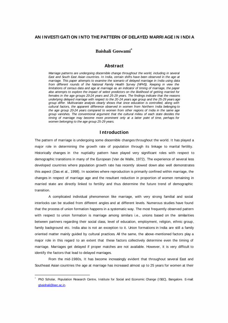
Coming to the educational attainment aspect of never married females, it is always believed
that with improvement s in educational status, the proportion of never married females coming under
each age group increases over time or in other words, marriages get delayed over time. From table 4
one can observe that for females with no education and those having higher education, the percentage
of never married females has increased between NFHS 1 and NFHS 3. However, with respect to the
other two categories, the scenario appears slightly different. Women with primary education show a
higher marriage rate resulting in a lower percentage of never married females in the age groups of 20-
24 and 25-29 years over time. The same holds true for women with secondary education also.
However, looking at the growth rate, it becomes clear that it is only during the first half that women
with no education reveal the highest as well as positive increments. However, in the later half, women
with higher education in age group of 20-24 and 25-29 years reveal highest increments.
6
Table 4: Percentage Share of Never Married Females by Highest Level of Education
Age
group 1992-93
(1) 1998-99
(2) 2005-06
(3)
Growth rate over (1) & (2)
Growth rate over (2) & (3)
No Education
15-19
20-24
25-29
37.6 (11326)
5.6 (13356)
1.7 (12676)
44.1 (8127)
7.3 (9734)
2.1 (10611)
50.3 (5615)
7.1 (7865)
1.7 (9529)
3.5
6.1
4.7
2.3
-0.5
-3.2
Primary
15-19
20-24
25-29
62.7 (5898)
14.2 (4905)
3.6 (4072)
63.7 (28472)
12.8 (3933)
3.5 (3634)
64.5 (4015)
13.2 (3451)
2.3 (3175)
0.4
-2.0
-0.6
0.2
0.5
-6.7
Secondary
15-19
20-24
25-29
82.2 (8944)
30.5 (6062)
7.8 (4007)
78.3 (11382)
22.2 (7324)
6.6 (5534)
83.8 (16184)
26.2 (11204)
5.6 (8490)
-1.0
-5.4
-3.0
1.2
3.0
-2.5
Higher
15-19
20-24
25-29
94.3 (460)
65.1 (1712)
20.0 (1357)
92.7 (2972)
55.3 (4221)
18.2 (2871)
94.5 (913)
69.2 (3120)
24.1 (2379)
-0.3
-3.0
-1.8
0.3
4.2
5.4
Note: Absolute figures are given in parentheses
Table 5: Percentage Share of Never Married Females by Highest Educational Level Attained
Age
group 1992-93
(1) 1998-99
(2) 2005-06
(3)
Growth rate over (1) & (2)
Growth rate over (2) & (3)
No Education
15-19
20-24
25-29
37.6 (11326)
5.6 (13356)
1.7 (12676)
44.1 (8127)
7.3 (9734)
2.1 (10611
50.3 (5615)
7.1 (7865)
1.7 (9529)
3.5
6.1
4.7
2.3
-0.5
-3.2
Incomplete Primary
15-19
20-24
25-29
60.1 (4326)
13.9 (3769)
3.6 (3229)
63.8 (2550)
13.0 (2121)
3.5 (2116)
67.3 (1972)
13.5 (1617)
2.7 (1673)
1.2
-1.3
-0.6
0.9
0.6
-3.8
Complete Primary
15-19
20-24
25-29
69.7 (1572)
15.2 (1135)
3.8 (844)
63.7 (1967)
12.7 (1811)
3.4 (1517)
61.7 (2043)
12.9 (1833)
1.7 (1502)
-1.7
-3.3
-2.1
-0.5
0.3
-8.3
Incomplete
Secondary
15-19
20-24
25-29
81.5 (7977)
27.2 (4946)
6.7 (3392)
77.6 (8779)
20.9 (5045)
6.0 (3789)
82.9 (14537)
23.4 (9953)
5.1 (7243)
-1.0
-4.6
-2.1
1.1
2.0
-2.5
Complete Secondary
15-19
20-24
25-29
87.9 (966)
45.0 (1116)
13.5 (615)
80.6 (2601)
25.2 (2279)
7.9 (1744)
91.1 (1648)
40.5 (1851)
8.5 (1247)
-1.7
-8.8
-8.3
2.2
10.1
1.3
Higher
15-19
20-24
25-29
94.3 (460)
65.1 (1712)
20.0 (1357)
92.7 (2972)
55.3 (4221)
18.2 (2871)
94.5 (913)
69.2 (3120)
24.1 (2379)
-0.3
-3.0
-1.8
0.3
4.2
5.4
Note: Absolute figures are given in parentheses

7
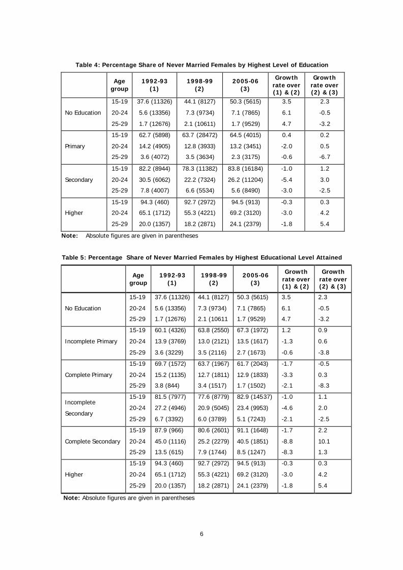
A further bifurcation of primary and secondary educational levels (table 5) into incomplete
primary and complete primary as well as incomplete secondary and complete secondary shows that for
women with incomplete primary education, the percentage of never married females remains almost
stable across all the age groups over the stipulated time period, whereas in the case of females with
complete primary and incomplete or complete secondary education, this proportion decreases especially
in the age groups of 20-24 and 25-29 years.
However by looking at the changes, it becomes evident that during the first half, females
belonging to most of the age groups exhibit a negative growth rate , whereas in the later half, females
coming under 20-24 age group with secondary education completed experience highest incremental
changes. On the whole, very nominal increments have been observed across different categories of
education.
Sex of the heads of households has also a role to play in determining the age at marriage of
individuals. It has been found that in male headed households, females get married earlier as compared
to those households headed by females across all the three age groups (table 6). The common reason
being that as most of the female headed households tend to be poverty stricken, and also the fact that
daughters’ marriage involves huge expenses (particularly in the form of dowry) in the Indian society,
these households may not be able to arrange the provisions for marriage at the proper time and hence
marriages get delayed. However a closer look into the incremental changes show that the incremental
increase in respect of never married females is more prominent among male headed households.
Table 6: Percentage share of never married females by sex of household head
Age
group 1992-93
(1) 1998-99
(2) 2005-06
(3)
Growth rate over (1) & (2)
Growth rate over (2) & (3)
Male
15-19
20-24
25-29
58.4 (24514)
15.8 (24134)
3.6 (20579)
66.7 (24622)
19.4 (23094)
4.8 (20843)
74.0 (23274)
23.1 (22679)
5.0 (20875)
2.8
4.6
6.6
1.8
3.2
0.7
Female
15-19
20-24
25-29
67.1 (2247)
29.8 (2006)
12.8 (1607)
71.9 (2391)
32.7 (2122)
12.4 (1816)
75.1 (3472)
29.2 (3013)
8.4 (2745)
1.4
2.0
-0.6
0.7
-1.8
-5.3
Note: Absolute figures are given in parentheses
Table 7 shows percentage share of never married females by caste of the heads of households
across three different periods. Despite an increase over time, the proportional changes are found higher
between NFHS 1 and 2 as compared to those between NFHS 2 and 3. High increments are seen among
women belonging to scheduled castes, scheduled tribes and other castes across 20-24 and 25-29 age
groups during the first half of the stipulated period. For the second half, women aged between 25-29
among scheduled tribes and other backward classes have exhibit negative increments.

8
Table 7: Percentage share of never married females by household caste
Age group
1992-93 (1)
1998-99 (2)
2005-06 (3)
Growth rate over (1) &(2)
Growth rate over (2) &(3)
Scheduled Caste
15-19
20-24
25-29
48.9 (3246)
9.7 (2989)
1.8 (2593)
60.8 (4865)
17.1 (4531)
4.1 (3990)
70.4 (5252)
18.5 (4939)
4.7 (4331)
4.8
15.2
25.6
2.7
1.3
2.5
Scheduled Tribe
15-19
20-24
25-29
52.6 (2258)
14.2 (2365)
4.3 (2044)
62.8 (2232)
18.6 (2144)
6.2 (2052)
68.1 (2341)
18.7 (2070)
5.2 (1865)
3.8
6.2
8.8
1.3
0.2
-2.7
Other Backward
Classes
15-19
20-24
25-29
NA
64.7 (8748)
18.1 (8280)
4.6 (7402)
72.7 (10737)
20.2 (10146)
4.1 (9545)
NA
2.0
2.0
-1.8
Other
15-19
20-24
25-29
61.4 (21255)
18.2 (20790)
4.6 (17554)
74.0 (9448)
25.2 (8909)
6.6 (7996)
81.7 (7508)
32.8 (7693)
7.0 (7153)
4.2
7.6
8.6
1.7
5.0
1.0
Note: Absolute figures are given in parentheses
Information on religion of the heads of households is available from NFHS 2 onwards. Table 8
shows the percentage shares of never married females by religion of the household head. As per NFHS
2 and 3, Christians reveal relatively higher percentages of never married population under each age
group.
Table 8: Percentage share of never married females by household religion
Age group NFHS 2 NFHS 3 Growth
Hindu
15-19
20-24
25-29
65.8 (21366)
19.1 (20168)
5.0 (18399)
73.3 (20844)
22.6 (20557)
5.1 (19096)
1.8
3.0
0.3
Muslim
15-19
20-24
25-29
67.9 (4051)
20.7 (3557)
5.7 (2858)
74.2 (4450)
23.2 (3718)
4.9 (3251)
1.5
2.0
-2.3
Christian
15-19
20-24
25-29
80.0 (711)
43.7 (661)
15.6 (662)
86.1 (577)
47.2 (568)
15.4 (512)
1.3
1.3
-0.2
Sikh
15-19
20-24
25-29
89.8 (432)
38.0 (445)
6.3 (366)
92.1 (443)
41.0 (468)
9.1 (384)
0.5
1.3
7.3
Others
15-19
20-24
25-29
80.1 (453)
34.2 (407)
7.3 (372)
82.4 (431)
35.4 (381)
9.3 (376)
0.5
0.7
4.5
Note: Absolute figures are given in parentheses

9
However, the incremental changes are more visible among Sikh women and women belonging
to other religions, especially for those coming under 25-29 age group.
Table 9 provides the percentage shares of never married female population in different states across
three selected age groups. It is very interesting to see that the percentage shares of never married
female population have increased over time across all the age groups in Jammu and Kashmir, Himachal
Pradesh, Delhi, Rajasthan, Uttar Pradesh (including Uttaranchal for 2005-06), Maharashtra and Tamil
Nadu. For states like Punjab, Haryana, Bihar (including Jharkhand for 2005-06), Orissa, Madhya Pradesh
(including Chhattisgarh for 2005-06), Gujarat and Karnataka incremental increases for the first half are
more evident, whereas for the second half, in respect of certain age groups, negative growth rates have
been observed. Surprisingly, in a state like Kerala, the percentage shares of never married females
across all the age groups have exhibit almost no change or negative increments.
Again a state like Andhra Pradesh, which has experienced very nominal changes for the first
half, reveals a sign of improvement for the second half, especially for those coming under 20-24 age
group. It has to be kept in mind that once the proportion of never married females reaches a certain
level, chances of further increments become rare, given the cultural landscape of India. Hence with
regard to states like Kerala, where the proportion of never married females were 43 percent and 12
percent for 20-24 and 25-29 age groups respectively (which are relatively higher as compared to a
majority of the Indian States) as early as in 1992-93, chances for further increments are few. What is
interesting to note here is the decline observed in the proportion of never married females across 20-24
and 25-29 age groups in Kerala over time.
Table 9: Percentage of never married females by major states, India
States 1992-93 (1)
1998-99 (2)
2005-06 (3)
growth (1) & (2)
growth (2) & (3)
Jammu and Kashmir 15-19 20-24 25-29
82.8(1009) 34.3(947) 6.1(834)
91.0(1072) 47.9(889) 14.0(878)
93.4(787) 62.6(688) 19.1(679)
2 7.93 25.82
0.43 5.12 6.11
Himachal Pradesh 15-19 20-24 25-29
83.6(1026) 22.4(964) 3.2(793)
94.2(873) 39.2(911) 5.1(790)
94.6(629) 41.4(677) 9.3(581)
2.52 14.98 12.12
0.08 0.92 13.93
Punjab 15-19 20-24 25-29
87.3(935) 32.2(894) 5.4(766)
91.6(813) 41.0(813) 7.7(672)
89.6(721) 39.3(866) 8.1(668)
1 5.43 8.91
-0.37 -0.69 0.74
Haryana 15-19 20-24 25-29
56.9(905) 9.7(868) 0.8(717)
75.4(776) 20.1(713) 2.5(681)
77.9(634) 17.6(580) 2.3(520)
6.5 21.45 39.66
0.56 -2.05 -1.26
Delhi 15-19 20-24 25-29
83.1(830) 28.7(970) 6.1(946)
89.7(726) 39.9(765) 6.9(648)
91.0(657) 45.4(736) 10.7(663)
1.57 7.82 2.65
0.25 2.3 9.03
Rajasthan 15-19 20-24 25-29
45.5(1499) 9.0(1349) 1.0(1218)
55.7(2153) 9.6(1918) 1.5(1622)
65.0(913) 13.5(845) 1.8(709)
4.5 1.22 10.04
2.76 6.77 3.99
Uttar Pradesh 15-19 20-24 25-29
60.4(3297) 10.2(3154) 1.1(2602)
64.8(3083) 13.1(2609) 2.2(2227)
79.7(3818)@ 22.5(3120)@ 3.6(2885)@
1.45 5.83 20.29
3.84 11.82 9.84
Bihar 15-19 20-24 25-29
41.9(1542) 8.5(1522) 2.2(1300)
60.0(1973) 12.4(1885) 2.4(1701)
58.8(1626)# 14.1(1407)# 2.1(1296)#
8.62 9.17 1.84
-0.32 2.4 -1.9

10
Assam 15-19 20-24 25-29
72.4(1028) 37.8(917) 13.2(842)
75.8(1031) 35.0(977) 15.9(904)
76.1(762) 36.1(846) 15.9(769)
0.93 -1.5 4.17
0.08 0.5 -0.07
West Bengal 15-19 20-24 25-29
56.6(1307) 18.7(1155) 7.0(1066)
61.3(1237) 19.3(1178) 7.3(1115)
61.3(1457) 18.1(1407) 5.9(1215)
1.65 0.61 0.65
0 -1.05 -3.07
Orissa 15-19 20-24 25-29
76.8(1302) 27.0(1320) 5.6(1122)
81.1(1278) 30.7(1153) 7.0(1228)
78.2(974) 34.3(956) 8.3(856)
1.11 2.77 4.94
-0.58 1.96 3.07
Madhya Pradesh 15-19 20-24 25-29
38.1(1721) 7.7(1772) 2.1(1434)
58.3(1845) 14.5(1791) 3.9(1653)
74.9(2202)$ 16.3(1981)$ 3.2(1851)$
10.65 17.55 17.01
4.75 2.05 -2.95
Gujarat 15-19 20-24 25-29
73.3(1094) 19.1(1207) 3.6(883)
76.7(1119) 21.9(1053) 4.4(815)
77.6(749) 27.0(795) 3.8(682)
0.92 2.92 4.38
0.19 3.88 -2.28
Maharashtra 15-19 20-24 25-29
62.7(1132) 17.2(1222) 4.5(994)
69.4(1645) 21.1(1530) 5.8(1404)
82.6(1797) 28.0(1923) 6.5(1802)
2.14 4.57 5.8
3.17 5.46 2.02
Andhra Pradesh 15-19 20-24 25-29
45.9(1217) 11.0(1112) 2.6(1015)
52.0(1053) 10.8(991) 2.6(884)
67.2(1304) 18.2(1381) 3.0(1368)
2.7 -0.32 0.31
4.85 11.5 2.53
Karnataka 15-19 20-24 25-29
61.3(1403) 22.7(1345) 6.0(1132)
66.4(1356) 25.4(1244) 7.6(1107)
76.6(1267) 27.2(1301) 7.2(1321)
1.66 2.4 5.26
2.56 1.19 -0.87
Kerala 15-19 20-24 25-29
84.1(1286) 43.3(1356) 12.4(1151)
84.4(813) 36.6(792) 10.3(775)
87.4(579) 36.9(621) 8.9(607)
0.06 -3.08 -3.38
0.6 0.12 -2.3
Tamil Nadu 15-19 20-24 25-29
74.3(1137) 24.6(1084) 7.0(951)
75.7(1112) 31.6(1226) 8.2(1106)
87.9(900) 37.0(1106) 9.9(1042)
0.38 5.7 3.36
2.68 2.81 3.36
Note: Absolute figures are given in parentheses; @ includes Uttaranchal; # includes Jharkhand; $
includes Chhattisgarh
Multivariate Analysis
In this section an attempt has been made to identify some of the predictors that may have implications
in terms of determining marital status in India. In what follows is a discussion on the plausible
explanatory variables and their linkages to marital status.
Issues and Hypotheses
The purpose of this section is to discuss certain basic personal (educational attainment), familial (place
of residence, sex of the head of the household) and socio-cultural (social composition of the population,
state) characteristics and their impact on female marriage in India.
Female Education and Transition to Marriage
A positive association is expected to be seen between educational attainment of females and their
transition to marriage. A woman with higher education is always more likely to remain unmarried at a
given point of time as compared to a woman with no education at the same given point of time. The
explanation can be twofold. First, the continuation of education delays the entry of a woman into the
marriage market. Second, education is often related to greater autonomy and opening up of new

11
avenues for women besides their familial and reproductive roles. They are expected to gain more
cont rol over household resources and personal behaviour (Dyson et al., 1983; Cain et al.,1979) so that
they can achieve better bargaining power in deciding the timing of their marriage as well as the
selection of their spouses.
However, the causality is not as simple as it apparently seems to be. Even though part of the
association between education and late marriage is explained with reference to a greater female
autonomy in the marriage process (Cochrane 1979), it ultimately depends on the social and cultural
context s within which these variables operate. For example, studies suggest that throughout South Asia,
education may serve to raise the value of daughters in transactions between households (Caldwell et
al., 1983); to make them more effective wives and mothers (Culpan et al., 1982) and hence, not
capable enough to alter the parents’ role in their daughter’s marriage (Fricke et al., 1986).
Familial factors
Place of residence impacts demographic outcomes. In diffusion theory, it has been argued that any
change in the demographic parameters starts from developed urban centres. Slowly the new behaviours
diffuse small cities, towns and ultimately the countryside. Even though there exist exceptions to this
theoretical proposition, in the present work, the type of place of residence has been factored in as one
of the explanatory variables. Sex of the head of the household also may decide the transition to
marriage. Most of the female headed households tend to be poverty stricken and thus face difficulties in
arranging the provisions for daughters’ marriage. Hence marriages sometimes get delayed for women in
female headed households.
Cultural parameters and marriage
In most of the developing context s, marriage is more of a cultural phenomenon rather than an
individual one in that personal happiness is generally given much lesser weight at the time of union
formation. However, as we know , it is not easy to capture cultural aspects quantitatively. Culture
reflects itself through other variables, for example, religion, caste etc. It has been well recognised in the
demographic literature that as part of culture, religion, in some special contexts, can influence a wide
range of social behaviours. Religious precepts could affect fertility, autonomy of women, their decision
making, access to economic resources and so on. For example, in India, several studies, by applying
multivariate techniques on secondary data, have found that Muslim population has a strong,
independent and positive effect on fertility (Bhat et al., 1990; Dreze et al., 2001; Chattopadhyay et al,
2004; Kulkarni et al., 2005). Coming to age at marriage, in India, it has been found that historically
Hindus and Muslims have had lower ages at marriage as compared to Christians. Keeping in view these
causations, religion has been considered as a proxy variable for culture. Again in almost all parts of
India marriages are caste endogamous. In the caste hierarchy, those who belong to the upper end have
a tendency to marry off their daughters early, sometimes even before they reach their puberty. Even
among scheduled castes, this trend is found. However, among certain tribes, pre-puberty marriages are
culturally uncommon. Even though things are changing, caste still plays a role in determining the timing
of marriages and hence included in the model as another proxy for culture. Lastly, the state which the

12
respondent s belong to, also shapes their cultural orientation. For instance, it has been found in the
literature that sometimes indicators like education can not explain the demographic outcomes the way a
state can. Researches reveal that the acceptance of family planning methods is more visible among the
least educated women of Kerala as compared to the highly educated women of Uttar Pradesh (McNay
et al, 2003). There may be some other dimensions of culture , but keeping in view the constraints of
data, the analysis has been confined within these three culture related parameters.
There are numerous other factors that we have not been able to capture in the present study.
For example, physical distance may represent a major constraint in terms of finding a suitable partner
and thereby leading to late marriages. It has been found in a French survey that spatial mobility plays a
central role in understanding the process of union formation. However, for estimating marriage market
from a spatial point of view, both the place of birth and place of residence of married couples are not
sufficient. Place of birth does not reflect the real pool of potential partners while the latter represents a
successive moment. Basically, information on the residence of each partner at each significant point in
time of t heir life cycle would be useful, but that is not available in the dataset.
Characteristics of local marriage markets influence the marriage timings both for men and
women. In the present work I could not include any explanatory variable as a proxy for the local
marriage market. Sex ratio of men and women at marriageable age is a very crude measure in this
regard and also which area can come under the local marriage market also is a debateable issue.
Several changes in marriage timing patterns depend, both cross-sectionally as well as
lontgitudinally, on exogenous factors like changes occurring in labour market, individual preferences for
career development, duration of economic crises and so on. directly affect marriage conditions.
However, keeping in view the limitations of the data, these factors could not be included in the model.
Results of Multivariate analysis
Table 10 present s the coefficients of the logistic regression categorising females into two selected age
groups 20-24 and 25-29. As compared to Hindus, women belonging to all other religious groups are
found to be significantly more likely to remain unmarried by age 20-24 years. Coming to caste, females
belonging Scheduled tribes and other castes have less chances to get married as compared to
scheduled caste females. However, women belonging to other backward classes do not reveal any
statistically significant relationship as far as chances of their getting married by age 20-24 are
concerned. As compared to women with no education, women coming under all other educational
categories have significantly lesser chances of getting married by age 20-24. As expected women
belonging to urban areas have fewer chances of getting married as compared to their rural
counterparts. Chances of getting married by age 20-24 are relatively lower for women belonging to
female headed households as compared to their counterparts in male headed households.
Coming to 25-29 age group, in relation to Hindu females, all women belonging to other
religious groups have fewer chances of getting married, albeit at a lower degree (except ing Muslim
women). Interestingly, as compared to women belonging to scheduled castes, females belonging to
other backward classes and other castes are significantly less likely to remain unmarried. However,
women belonging to scheduled tribes do not reveal any statistically significant relationship as far as

13
chances of getting married by age 25-29 are concerned. Under this age group, women with primary
education do not exhibit any statistically significant relationship as compared to women with no
education, as far as the likelihood of getting married is concerned.
Table 10: Coefficients of Logistic Regression model
20-24 25-29
Coefficient Std. Error Coefficient Std. Error
Religion (Ref: Hindu) Muslim Christian Sikh Others Caste (Ref: Scheduled Caste) Scheduled Tribe OBC Others Educational attainment (Ref: No Education) Primary Secondary Higher Place of Residence (Ref: Rural) Urban Sex of Household Head (Ref: Male) Female Age Constant
.199*** .681*** .520*** .591*** .220** -.063 .153*** .689*** 1.448*** 3.344*** .551*** .456*** -.478*** 7.366***
.056 .127 .136 .134 .088 .055 .054 .079 .061 .074 .041 .054 .014 .318
.304*** .401** .442** .448** .054 -.339*** -.360*** .218 .972*** 2.620*** .565*** .610*** -.313*** 4.108***
.101 .186 .213 .187 .157 .098 .093 .159 .108 .114 .075 .083 .024 .652
Dependent Variable: Marital Status (0- Currently Married; 1- Never Married)
*** 1 % level of significance; ** 5 % level of significance
However, in respect of other categories, the chances of women remaining unmarried are
significantly higher in relation to women with no education. Women residing in urban areas experience
fewer chances of getting married as compared to their rural counterparts. Under 25-29 age group also,
women hailing from female headed households reveal fewer chances of getting married as compared to
their counterparts belonging to male headed households.
It is already mentioned that state also has been considered as one of the explanatory variables
in order to capture different cultural milieu of each state. Table 11 present s the coefficients of state in
the same regression model for two age groups separately. Considering Kerala as the reference state, it
has been found that females in states like Jammu and Kashmir, Himachal Pradesh, Assam, Orissa, Tamil

14
Nadu are less prone to getting married under both models. There are some states which demonstrate a
significant relationship with respect to one age group but not the other. For example, under 20-24 age
group, females in Punjab, Delhi and Karnataka (at a lower degree) are less likely to get married as
compared to females belonging to the reference state. However, in respect of 25-29 age group, no
statistically significant relationship has been found. Women in Haryana and Rajasthan are significantly
less likely to remain unmarried under both models. Women in states like Bihar (including Jharkhand),
Madhya Pradesh (including Chhattisgarh) and Andhra Pradesh are also less likely to remain unmarried
as compared to those belonging to the reference state. However, for Bihar (including Jharkhand) the
coefficient is not significant in respect of 20-24 age group, for Madhya Pradesh (including Chhattisgarh)
under 25-29 age group and for Andhra Pradesh under both the age groups. With respect to states like
Uttar Pradesh (including Uttaranchal), Gujarat and Maharashtra, the coefficients are statistically
insignificant under both the models.
Table 11: Coefficients of state under Logistic Regression model
20-24 25-29
States Coefficient Std. Error Coefficient Std. Error
Kerala
Jammu and Kashmir
Himachal Pradesh
Punjab
Haryana
Delhi
Rajasthan
Uttar Pradesh@
Bihar#
Assam
West Bengal
Orissa
Madhya Pradesh$
Gujarat
Maharashtra
Andhra Pradesh
Karnataka
Tamil Nadu
Ref
1.444***
.783***
.523***
-.563***
.342**
-.451***
.110
-.212
.968***
.207
.894***
-.239*
.180
.060
-.189
.220*
.406***
.163
.141
.154
.163
.139
.156
.115
.131
.140
.129
.132
.124
.140
.120
.124
.129
.127
Ref
1.111***
.609***
.232
-.892***
.224
-.715**
-.203
-.660***
1.635***
.618***
.982***
-.335
-.322
.193
-.001
.313
.420**
.235
.224
.258
.358
.224
.316
.195
.248
.209
.209
.214
.214
.271
.195
.206
.209
.209
Dependent Variable: Marital Status (0- Currently Married; 1- Never Married)
*** 1 % level of significance; ** 5% level of significance; * 10% level of significance @ includes Uttaranchal; #includes Jharkhand; $ includes Chhattisgarh

15
Discussion
These findings provide an indication of the pattern of delayed marriages in India. As expected, that
section of the population educated beyond a threshold level, has been found delaying marriage even at
age 25-29. Coming to religious identities, it has been found that religious identity plays an important
role in determining the marital status in respect of both the age groups. However, identities related to
ethnic groups exhibit different trends under the two models. Women belonging to other castes are
significantly more likely to remain unmarried at age 20-24, whereas under 25-29 age group, they are
significantly less likely to remain unmarried as compared to women belonging to scheduled castes. It
hints towards the fact that the reasons underlying delayed marriages with respect to 20-24 and 25-29
age groups might be different. Higher chances of women remaining unmarried in female-headed
households in respect of both the age groups, once again reconfirms the fact that female heads are
unable to make provisions for daughters’ marriage at the proper time perhaps due to the widely
prevalent system of dowry. Moreover, sometimes, even though enough resources are available the
absence of father-figures might hamper the initiatives in terms of arranging marriages of eligible
unmarried girls in the families.
Alt hough state has been considered as one of the explanatory variables in the logistic
regression framework, it is very difficult to say anything precisely based on these coefficients. It is
evident from the bivariate analysis that in Kerala, the percentage of never married female population
has declined over time. Based on the multivariate analysis, females in the bordering states show greater
chances of remaining unmarried under both the models as compared to women in Kerala. Females from
states like Haryana and Rajasthan have reveal greater chances of getting married, perhaps owing to
their very traditional and patriarchal environment. The reason for some of state coefficients being
significant under the first model and insignificant under the second (e.g., Punjab, Delhi, Karnataka and
Madhya Pradesh (including Chhattisgarh)) might be a reduction in the number of cases with regard to
that particular age group. In a country like India, where marriage is universal, we rarely come across
women remaining unmarried throughout their life. By age 25-29, only a small proportion of women
remain unmarried rendering the predictors insignificant sometimes.
Furthermore, the coefficient for West Bengal is insignificant under the first model, whereas it is
significantly positive under the second model. Similarly, the coefficient for Bihar (including Jharkhand)
also is insignificant under the first model and significantly negative under the second model. It hints
towards the fact that once a factor like education is cont rolled, the apparent disadvantages observed of
the northern states may vanish at least with respect to 20-24 age group. Moreover, the conventional
argument that the cultural factors of different states decide the timing of marriages may become
applicable at a later stage. That is why for females in Bihar (including Jharkhand) the chances of
remaining unmarried at age 25-29 is significantly lower as compared to Kerala. However, it remains
difficult to say anything precisely with regard to the coefficient of West Bengal. It may be the urban
female population which makes a diffe rence, as according to 2001 census, urban fertility is the lowest in
West Bengal.
What appears more difficult to determine is why females in Assam and Orissa reveal
significantly higher chances of remaining unmarried across both the age groups. In the case of Orissa,

16
the same argument, in line with female headed households can be put forth. This is one of the poorest
states in India where the social environment is still very traditional and the prevalence of dowry evil is
rampant. Hence, it may so happen that marriages get delayed because of the inability to attract
partners from the same social classes of the population. However, it is difficult to test this proposition.
Conclusion
From the above findings it can be safely asserted that even at the country level, marriages get delayed
in respect of the upper section of the population in the context of education, the pattern of delayed
marriages at the state level might have taken a different route altogether. It is very difficult to draw any
definitive conclusions with respect to the states based on the present analysis, as the socio-economic
environment s differ substantially from one state to another. Some states are economically progressive,
while some others have achieved remarkable improvement s with regard to social indicators. In some
states, the cultural environment is still very traditional, whereas, some have adapted to new lifestyles
even while holding on to traditional values. Moreover, in some states, changes in socio-demographic
indicators are very fast and drastic and some are moving steadily towards better positions. Each of the
predictors may work differently in each state depending on the cultural set-up as well as the transitional
process they are passing through. Given this scenario, it is almost impossible to come up with a general
conclusion.
However, one major conclusion of this exercise may run against the conventional notion that
marriage timing is a cultural phenomenon in the Indian context . It has been found that once education
is controlled along with cultural factors, women in states like Bihar (including Jharkhand), Uttar Pradesh
(including Uttaranchal) in the northern region, Gujarat, Maharashtra in the western region and
Karnataka in the southern region are statistically not different from women in Kerala. It paves the way
for arguing that the spread of education does make a contribution towards delaying marriages at least
in the case of females belonging to 20-24 age group. Culture may be the prime explanatory factor at a
later stage, may be for women belonging to 25-29 age groups.
References
Agarwala, S N (1962). Age at Marriage in India. Allahabad: Kitab Mahal.
————— (1972). India’s Population Problems. Bombay: Tata McGraw -Hill.
Basavarajappa, K G and M I Belvalgidad (1967). Changes in Age at Marriage of Females and Their
Effect on the Birth Rate in India. Eugenics Quartrely 14 (1):14-26.
Bhat P N M and S Irudaya Rajan (1990). Demographic Transition in Kerala Revisited. Economic and
Political Weekly, 25 (35 & 36): 1957-80.
Chattopadhyay, A, R B Bhagat and T K Roy (2004). Hindu-Muslim Fertility Differentials: A Comparative
Study of Selected States of India. In T K Roy, M Guruswamy and Arokiaswamy (eds),
Population, Development and Health: A Changing Perspective. Jaipur and New Delhi: Rawat
Publishers. 138-156.

17
Cain, M, S R Khanum and S Nahar (1979). Class, Patriarchy, and Women’s Wotk in Bangladesh.
Population and Development Review, 5: 405-38.
Caldwell, J C, P H Reddy, and P Caldwell (1983). The Causes of Marriage Change in South India.
Population Studies, 27: 343-61.
Cochrane, S L (1979). Fertility and Education: What Do We Really Know?. Baltimore, Md: Johns Hopkins
University Press.
Culpan Oya and Toni Marzotto (1982). Changing Attitude toward Work and Marriage: Turkey in
Transition. Signs, 8 (2): 337-51.
Das, N P and Devamoni Dey (1998). Female Age at Marriage in India: Trends and Determinants.
Demography India, 27 (1): 91-115.
Dreze, J and Murthi M (2001). Fertility, Education and Development: Evidence from India. Population
and Development Review, 27 (1): 171-220.
Dyson, T and M Moore (1983). On Kinship Structure, Female Autonomy, and Demographic Behaviour in
India. Population and Development Review, 9: 35-60.
Fricke, Thomas E, Sabiha H Syed and Peter C Smith (1986). Rural Punjabi Social Organization and
Marriage Timing Strategies in Pakistan. Demography, 23 (4): 489-508.
Goyal, R P (1988). Marriage Age in India. Delhi: B R Publishing House.
Jones, Gavin W (2004). Not ‘when to marry’ but ‘whether to marry’: the Changing context on Marriage
Decisions in East and Southeast Asia. In G W Jones and K Ramdas (ed), (Un)tying the Knot:
Ideal and Reality in Asian Marriage. Singapore: Asia Research Institute, National University of
Singapore.
Kulkarni, P M and M Alagrajan (2005). Population Growth, Fertility and Religion in India. Economic and
Political Weekly, 40 (5): 403-410.
Leete, R (1994). The Continuing Flight from Marriage and Parenthood among the Overseas Chinese in
East and Southeast Asia: Dimensions and Implications. Population and Development Review,
20 (4): 811-29.
Lesthaeghe, R (2010). The Unfolding Story of Second Demographic Transition. Population and
Development Review, 36 (2): 211-51.
Malaker, C R (1972). Female Age at Marriage and Birth Rate in India. Social Biology, 19: 297-301.
Malaker, C R (1973). Construction of Nuptiality Tables for Single Population of India: 1901-1931.
Demography, 10: 525-35.
Malaker, C R (1975). Socio-economic and Demographic Correlates of Marriage Patterns in India.
Demography India, 4: 317-48
McNay, K, P Arokiasamy and Robert H Cassen (2003). Why are Uneducated Women in India using
Contraception? A multilevel Analysis. Population Studies, 57 (1): 21-40.
Van de Walle, Etienne (1972). Marriage and Marital Fertility. In D V Glass and Roger Revelle (eds),
Population and Social Change. Edward Arnold.
18
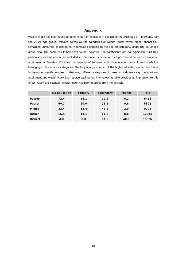
Appendix
Wealth Index has been found to be an important indicator in explaining the likelihood of marriage. For
the 20-24 age group, females across all the categories of wealth index reveal higher chances of
remaining unmarried as compared to females belonging to the poorest category. Under the 25-29 age
group also, the same result has been found, however, the coefficients are not significant. But this
particular indicator cannot be included in the model because of its high correlation with educational
attainment of females. Moreover, a majority of females with no education come from households
belonging to the poorest categories. Similarly a large number of the highly educated women are found
in the upper wealth quintiles. In that way, different categories of these two indicators e.g., educational
attainment and wealth index just replace each other. The following table provides an impression to this
effect. Given this scenario, wealth index has been dropped from the analysis.
No Education Primary Secondary Higher Total
Poorest
Poorer
Middle
Richer
Richest
72.4
50.7
33.4
16.4
4.3
15.1
20.6
18.4
13.1
3.8
12.2
28.1
45.3
61.6
51.6
0.2
0.6
2.9
8.8
40.3
5415
6821
9305
12344
15626
216 Technological Progress, Scale Effect andTotal Factor Productivity Growth inIndian Cement Industry: PanelEstimation of Stochastic ProductionFrontierSabuj Kumar Mandal and S Madheswaran
217 Fisheries and Livelihoods in TungabhadraBasin, India: Current Status and FuturePossibilitiesManasi S, Latha N and K V Raju
218 Economics of Shrimp Farming: AComparative Study of Traditional Vs.Scientific Shrimp Farming in West BengalPoulomi Bhattacharya
219 Output and Input Efficiency ofManufacturing Firms in India: A Case ofthe Indian Pharmaceutical SectorMainak Mazumdar, Meenakshi Rajeevand Subhash C Ray
220 Panchayats, Hariyali Guidelines andWatershed Development: Lessons fromKarnatakaN Sivanna
221 Gender Differential in Disease Burden: It’sRole to Explain Gender Differential inMortalityBiplab Dhak and Mutharayappa R
222 Sanitation Strategies in Karnataka: AReviewVeerashekharappa and Shashanka Bhide
223 A Comparative Analysis of Efficiency andproductivity of the Indian PharmaceuticalFirms: A Malmquist-Meta-FrontierApproachMainak Mazumdar and Meenakshi Rajeev
224 Local Governance, Patronage andAccountability in Karnataka and KeralaAnand Inbanathan
225 Downward Dividends of GroundwaterIrrigation in Hard Rock Areas of SouthernPeninsular IndiaAnantha K H
226 Trends and Patterns of Private Investmentin IndiaJagannath Mallick
227 Environmental Efficiency of the IndianCement Industry: An Interstate AnalysisSabuj Kumar Mandal and S Madheswaran
228 Determinants of Living Arrangements ofElderly in Orissa: An AnalysisAkshaya Kumar Panigrahi
229 Fiscal Empowerment of Panchayats inIndia: Real or Rhetoric?M Devendra Babu
230 Energy Use Efficiency in Indian CementIndustry: Application of DataEnvelopment Analysis and DirectionalDistance FunctionSabuj Kumar Mandaland S Madheswaran
231 Ethnicity, Caste and Community in aDisaster Prone Area of OrissaPriya Gupta
232 Koodankulam Anti-Nuclear Movement: AStruggle for Alternative Development?Patibandla Srikant
233 History Revisited: Narratives on Politicaland Constitutional Changes in Kashmir(1947-1990)Khalid Wasim Hassan
234 Spatial Heterogeneity and PopulationMobility in IndiaJajati Keshari Parida and S Madheswaran
235 Measuring Energy Use Efficiency inPresence of Undesirable Output: AnApplication of Data Envelopment Analysis(DEA) to Indian Cement IndustrySabuj Kumar Mandaland S Madheswaran
236 Increasing trend in Caesarean SectionDelivery in India: Role of Medicalisationof Maternal HealthSancheetha Ghosh
237 Migration of Kashmiri Pandits:Kashmiriyat Challenged?Khalid Wasim Hassan
238 Causality Between Energy Consumptionand Output Growth in Indian CementIndustry: An Application of Panel VectorError Correction ModelSabuj Kumar Mandal and S Madheswaran
239 Conflict Over Worship:A Study of the SriGuru Dattatreya Swami BababudhanDargah in South IndiaSudha Sitharaman
240 Living Arrangement Preferences of theElderly in Orissa, IndiaAkshaya Kumar Panigrahi
241 Challenges and Pospects in theMeasurement of Trade in ServicesKrushna Mohan Pattanaik
242 Dalit Movement and Emergence of theBahujan Samaj Party in Uttar Pradesh:Politics and PrioritiesShyam Singh
243 Globalisation, DemocraticDecentralisation and Social Secutiry inIndiaS N Sangita and T K Jyothi
244 Health, Labour Supply and Wages: ACritical Review of LiteratureAmrita Ghatak
245 Is Young Maternal Age A Risk Factor forSexually Transmitted Diseases andAnemia in India? An Examination inUrban and Rural AreasKavitha N
246 Patterns and Determinants of FemaleMigration in India: Insights from CensusSandhya Rani Mahapatro
247 Spillover Effects from MultinationalCorporations: Evidence From West BengalEngineering IndustriesRajdeep Singha and K Gayithri
248 Effectiveness of SEZs Over EPZsStructure: The Performance atAggregate LevelMalini L Tantri
Recent Working Papers

249 Income, Income Inequality and MortalityAn empirical investigation of therelationship in India, 1971-2003K S James and T S Syamala
250 Institutions and their Interactions:An Economic Analysis of IrrigationInstitutions in the Malaprabha DamProject Area, Karnataka, IndiaDurba Biswas and L Venkatachalam
251 Performance of Indian SEZs: ADisaggregated Level AnalysisMalini L Tantri
252 Banking Sector Reforms and NPA:A study of Indian Commercial BanksMeenakshi Rajeev and H P Mahesh
253 Government Policy and Performance: AStudy of Indian Engineering IndustryRajdeep Singha and K Gayithri
254 Reproduction of Institutions throughPeople’s Practices: Evidences from aGram Panchayat in KeralaRajesh K
255 Survival and Resilience of Two VillageCommunities in Coastal Orissa: AComparative Study of Coping withDisastersPriya Gupta
256 Engineering Industry, CorporateOwnership and Development: Are IndianFirms Catching up with the GlobalStandard?Rajdeep Singha and K Gayithri
257 Scheduled Castes, Legitimacy and LocalGovernance: Continuing Social Exclusionin PanchayatsAnand Inbanathan and N Sivanna
258 Plant-Biodiversity Conservation inAcademic Institutions: An EfficientApproach for Conserving BiodiversityAcross Ecological Regions in IndiaSunil Nautiyal
259 WTO and Agricultural Policy in KarnatakaMalini L Tantri and R S Deshpande
260 Tibetans in Bylakuppe: Political and LegalStatus and Settlement ExperiencesTunga Tarodi
261 Trajectories of China’s Integration withthe World Economy through SEZs: AStudy on Shenzhen SEZMalnil L Tantri
262 Governance Reforms in Power Sector:Initiatives and Outcomes in OrissaBikash Chandra Dash and S N Sangita
263 Conflicting Truths and ContrastingRealities: Are Official Statistics onAgrarian Change Reliable?V Anil Kumar
264 Food Security in Maharashtra: RegionalDimensionsNitin Tagade
265 Total Factor Productivity Growth and ItsDeterminants in Karnataka AgricultureElumalai Kannan
266 Revisiting Home: Tibetan Refugees,Perceptions of Home (Land) and Politicsof ReturnTarodi Tunga
267 Nature and Dimension of Farmers’Indebtedness in India and KarnatakaMeenakshi Rajeev and B P Vani
268 Civil Society Organisations andElementary Education Delivery in MadhyaPradeshReetika Syal
269 Burden of Income Loss due to Ailment inIndia: Evidence from NSS DataAmrita Ghatak and S Madheswaran
270 Progressive Lending as a DynamicIncentive Mechanism in MicrofinanceGroup Lending Programmes: EmpiricalEvidence from IndiaNaveen Kumar K and Veerashekharappa
271 Decentralisation and Interventions inHealth Sector: A Critical Inquiry into theExperience of Local Self Governments inKeralM Benson Thomas and K Rajesh
272 Determinants of Migration andRemittance in India: Empirical EvidenceJajati Keshari Parida and S Madheswaran
273 Repayment of Short Term Loans in theFormal Credit Market: The Role ofAccessibility to Credit from InformalSourcesManojit Bhattacharjee and Meenkashi Rajeev
274 Special Economic Zones in India: Arethese Enclaves Efficient?Malini L Tantri
Price: Rs. 30.00 ISBN 978-81-7791-131-2
INSTITUTE FOR SOCIAL AND ECONOMIC CHANGEDr V K R V Rao Road, Nagarabhavi P.O., Bangalore - 560 072, India
Phone: 0091-80-23215468, 23215519, 23215592; Fax: 0091-80-23217008E-mail: [email protected]; Web: www.isec.ac.in