an introduction to real analysis - geneseo.edu
TRANSCRIPT

An Introduction
to
Real Analysis
Cesar O. Aguilar
November 15, 2021


Contents
1 Preliminaries 1
1.1 Sets, Numbers, and Proofs . . . . . . . . . . . . . . . . . 1
1.2 Functions . . . . . . . . . . . . . . . . . . . . . . . . . . 5
1.3 Mathematical Induction . . . . . . . . . . . . . . . . . . 10
1.4 Countability . . . . . . . . . . . . . . . . . . . . . . . . . 15
2 The Real Numbers 25
2.1 Introduction . . . . . . . . . . . . . . . . . . . . . . . . . 25
2.2 Algebraic and Order Properties . . . . . . . . . . . . . . 29
2.3 The Absolute Value . . . . . . . . . . . . . . . . . . . . . 34
2.4 The Completeness Axiom . . . . . . . . . . . . . . . . . 42
2.5 Applications of the Supremum . . . . . . . . . . . . . . . 53
2.6 Nested Interval Theorem . . . . . . . . . . . . . . . . . . 58
3 Sequences 63
3.1 Limits of Sequences . . . . . . . . . . . . . . . . . . . . . 63
3.2 Limit Theorems . . . . . . . . . . . . . . . . . . . . . . . 75
3.3 Monotone Sequences . . . . . . . . . . . . . . . . . . . . 84
3.4 Bolzano-Weierstrass Theorem . . . . . . . . . . . . . . . 92
3.5 limsup and liminf . . . . . . . . . . . . . . . . . . . . . . 99
3.6 Cauchy Sequences . . . . . . . . . . . . . . . . . . . . . . 105
3

3.7 Infinite Series . . . . . . . . . . . . . . . . . . . . . . . . 111
4 Limits 129
4.1 Limits of Functions . . . . . . . . . . . . . . . . . . . . . 129
4.2 Limit Theorems . . . . . . . . . . . . . . . . . . . . . . . 139
5 Continuity 145
5.1 Continuous Functions . . . . . . . . . . . . . . . . . . . . 145
5.2 Combinations of Continuous Functions . . . . . . . . . . 151
5.3 Continuity on Closed Intervals . . . . . . . . . . . . . . . 155
5.4 Uniform Continuity . . . . . . . . . . . . . . . . . . . . . 162
6 Differentiation 169
6.1 The Derivative . . . . . . . . . . . . . . . . . . . . . . . 169
6.2 The Mean Value Theorem . . . . . . . . . . . . . . . . . 179
6.3 Taylor’s Theorem . . . . . . . . . . . . . . . . . . . . . . 184
7 Riemann Integration 193
7.1 The Riemann Integral . . . . . . . . . . . . . . . . . . . 193
7.2 Riemann Integrable Functions . . . . . . . . . . . . . . . 204
7.3 The Fundamental Theorem of Calculus . . . . . . . . . . 211
7.4 Riemann-Lebesgue Theorem . . . . . . . . . . . . . . . . 213
8 Sequences of Functions 215
8.1 Pointwise Convergence . . . . . . . . . . . . . . . . . . . 216
8.2 Uniform Convergence . . . . . . . . . . . . . . . . . . . . 224
8.3 Properties of Uniform Convergence . . . . . . . . . . . . 231
8.4 Infinite Series of Functions . . . . . . . . . . . . . . . . . 240
9 Metric Spaces 253
9.1 Metric Spaces . . . . . . . . . . . . . . . . . . . . . . . . 253

9.2 Sequences and Limits . . . . . . . . . . . . . . . . . . . . 261
9.3 Continuity . . . . . . . . . . . . . . . . . . . . . . . . . . 270
9.4 Completeness . . . . . . . . . . . . . . . . . . . . . . . . 277
9.5 Compactness . . . . . . . . . . . . . . . . . . . . . . . . 289
9.6 Fourier Series . . . . . . . . . . . . . . . . . . . . . . . . 294
10 Multivariable Differential Calculus 301
10.1 Differentiation . . . . . . . . . . . . . . . . . . . . . . . . 301
10.2 Differentiation Rules and the MVT . . . . . . . . . . . . 312
10.3 High-Order Derivatives . . . . . . . . . . . . . . . . . . . 318
10.4 Taylor’s Theorem . . . . . . . . . . . . . . . . . . . . . . 328
10.5 The Inverse Function Theorem . . . . . . . . . . . . . . . 332


Preface
The material in these notes constitute my personal notes that are used
in the course lectures for MATH 324 and 325 (Real Analysis I, II).
You will find that the lectures and these notes are very closely aligned.
The notes highlight the important ideas and examples that you should
master as a student. You may find these notes useful if:
• you miss a lecture and need to know what was covered,
• you want to know what material you are expected to master,
• you want to know the level of difficulty of questions that you
should expect in a test, and
• you want to see more worked out examples in addition to those
worked out in the lectures.
If you find any typos or errors in these notes, no matter how small,
please email me a short description (with a page number) of the typo/error.
Suggestions and comments on how to improve the notes are also wel-
comed.
Cesar Aguilar
SUNY Geneseo

1
Preliminaries
1.1 Sets, Numbers, and Proofs
We recall some basic set operations and introduce some notation. Let
A and B be subsets of a set S.
• Union of sets: A ∪B = {x ∈ S | x ∈ A or x ∈ B}
• Intersection of sets: A ∩B = {x ∈ S | x ∈ A and x ∈ B}
• Set complement: S\B = {x ∈ S | x /∈ B} = Bc
• To prove that A = B we must show that A ⊂ B and B ⊂ A.
• The empty set is denoted by ∅.
• The sets A and B are disjoint if A ∩ B = ∅.
• The Cartesian product of A and B, denoted by A× B, is the
set of ordered pairs (a, b) where a ∈ A and b ∈ B, in other words,
A× B = {(a, b) | a ∈ A, b ∈ B}.
• For any set S, the power set of S is the set of all subsets of S,
and is denoted by P(S).
1

1.1. SETS, NUMBERS, AND PROOFS
Below is the set of numbers that we will use in this book:
• The natural numbers: N := {1, 2, 3, 4, . . .}
• The integers: Z := {. . . ,−3,−2,−1, 0, 1, 2, 3, . . .}
• The rational numbers: Q :={ab | a, b ∈ Z, b 6= 0
}
• The real numbers: R
• The irrational numbers: R\Q
• We have the following chain of set inclusions:
N ⊂ Z ⊂ Q ⊂ R
The main methods of proof used in this book are the following:
• Direct Proof : To prove the statement “P ⇒ Q”, assume that
the statement P is true and show by combining axioms, defini-
tions, and earlier theorems that Q is true. This should be the
first method you attempt and
• Mathematical Induction: Covered in Section 1.3.
• By Contraposition: Proving the statement “P ⇒ Q” by prov-
ing the logically equivalent statement “not Q⇒ not P”. Do not
confuse this with proof by contradiction.
• By Contradiction: To prove the statement “P ⇒ Q”, assume
that P is true and show that some logical contradiction occurs.
This frequently gets confused with proof by contraposition in the
following way (do not do this): To prove that “P ⇒ Q”, assume
that P is true and suppose that Q is not true. After some work
2

1.1. SETS, NUMBERS, AND PROOFS
using only the assumption that Q is not true you show that P
is not true and thus you say that there is a contradiction because
you assumed that P is true. What you have really done is proved
the contrapositive. Thus, if you believe that you are proving a
statement by contradiction, take a close look at your proof to see
if what you have is a proof by contraposition.
Below is an example of a proper proof by contradiction.
Theorem 1.1.1
If x and y are consecutive integers then x+ y is odd.
Proof. Assume that x and y are consecutive integers (i.e. assume P )
and assume that x + y is not odd (i.e. assume not Q). Since x + y is
not odd then x + y 6= 2n + 1 for all integers n. However, since x and
y are consecutive, and assuming without loss of generality that x < y,
we have that x+ y = 2x+1. Thus, we have that x+ y 6= 2n+1 for all
integers n and also that x+ y = 2x+ 1. Since x is an integer we have
reached a contradiction. Hence, if x and y are consecutive integers then
x+ y is odd.
3

1.1. SETS, NUMBERS, AND PROOFS
Exercises
Exercise 1.1.1. Find the power set of S = {x, y, z, w}.
Exercise 1.1.2. Let A = {11, 22, 33} and let B = {1,−1}. Find A×B.
Exercise 1.1.3. Prove that if x and y are even natural numbers then
xy is also even. Do not use proof by contradiction.
Exercise 1.1.4. If x and y are rational numbers then x+y is a rational
number. Do not use proof by contradiction.
4

1.2. FUNCTIONS
1.2 Functions
A function f with domain A and co-domain B is a rule that assigns
to each element x ∈ A a unique element y ∈ B. We usually denote a
function with the notation f : A→ B, and the assignment of x to y is
written as y = f(x). We also say that f is a mapping from A to B, or
that f maps A into B. The unique element y assigned to x is called
the image of x under f . The range of f , denoted by f(A), is the set
f(A) = {y ∈ B | ∃ x ∈ A, y = f(x)}.
Example 1.2.1. Consider the mapping f : R → R defined by
f(x) =
1, x ∈ Q
−1, x ∈ R\Q.
The image of x = 1/2 under f is f(1/2) = 1. The range of f is
f(A) = {1,−1}.
Example 1.2.2. Consider the function f : N → P(N) defined by
f(n) = {1, 2, . . . , n}.
The set S = {2, 4, 6, 8, . . . , } of even numbers is an element of the co-
domain P(N) but is not in the range of f . As another example, the set
N ∈ P(N) itself is not in the range of f .
Definition 1.2.3: Surjection
A function f : A → B is said to be a surjection or is surjective
if every element of B is the image of some element of A. In other
words, for any y ∈ B there exists x ∈ A such that f(x) = y.
Equivalently, f : A→ B is surjective if f(A) = B.
5

1.2. FUNCTIONS
Example 1.2.4. The function f : R → R defined by f(x) = x2 is
not a surjection. For example, y = −1 is not in the range of f since
f(x) = x2 6= −1 for all x ∈ R. The range of f is f(R) = [0,∞).
Example 1.2.5. Consider the function f : R → R defined by f(x) =
arctan(x). The range of f is f(R) = (−π/2, π/2), and thus f is not a
surjection.
Example 1.2.6. Consider the function f : P(N) → N defined by
f(S) = min(S)
where min(S) denotes the smallest element of S ∈ P(N). Prove that f
is a surjection.
Proof. To prove that f is a surjection, we must show that for any
element y ∈ N (the co-domain), there exists S ∈ P(N) (the domain)
such that f(S) = y. Consider then an arbitrary y ∈ N. Let S = {y}and thus clearly S ∈ P(N). Moreover, it is clear that min(S) = y and
thus f(S) = min(S) = y. This proves that f is a surjection.
Notice that in Example 1.2.6, given any y ∈ N there are many sets
S ∈ P(N) such that f(S) = y. This leads us to the following definition.
Definition 1.2.7: Injection
A function f : A → B is said to be an injection or is injective if
no two distinct elements of A are mapped to the same element in
B, in other words, given any x1, x2 ∈ A, if x1 6= x2 then f(x1) 6=f(x2). Equivalently, f is injective if whenever f(x1) = f(x2) then
necessarily x1 = x2.
Example 1.2.8. The function f : R → R defined by f(x) = x2 is not
an injection. For example, f(−2) = f(2) = 4.
6
1.2. FUNCTIONS
Example 1.2.9. Consider again the function f : N → P(N) defined
by
f(n) = {1, 2, . . . , n}.
This function is an injection. Indeed, if f(n) = f(m) then {1, 2, . . . , n} =
{1, 2, . . . , m} and therefore n = m. Hence, whenever f(n) = f(m) then
necessarily n = m and this proves that f is an injection.
Example 1.2.10. Consider the function f : P(N) → N defined by
f(S) = min(S)
Is f an injection?
Example 1.2.11. Consider the function f(x) = sin(x) with domain
A = R. The function f is not injective. For example, for any integer k ∈Z it holds that f(kπ) = 0. For example, f(3π) = f(2π) = f(−5π) = 0.
Example 1.2.12. Consider the function f : N → P(N) defined by
f(n) = {n}
This function is an injection.
Definition 1.2.13: Bijection
A function f : A → B is said to be a bijection if it is a surjection
and an injection.
Example 1.2.14. Suppose that f : P → Q is an injection. Prove that
the function f : P → f(P ) defined by f(x) = f(x) for x ∈ P is a
bijection.
7

1.2. FUNCTIONS
Solution. By construction, f is a surjection. If f(x) = f(y) then f(x) =
f(y) and then x = y since f is an injection. Thus, f is an injection and
this proves that f is a bijection.
Example 1.2.15. Prove that f : Q\{0} → Q\{0} defined by f(pq) =qp
is a bijection, where gcd(p, q) = 1.
8

1.2. FUNCTIONS
Exercises
Exercise 1.2.1. Consider the function f : N → Q defined by f(n) = 1n.
Is f an injection? Is f a surjection?
Exercise 1.2.2. Consider the function f : N × N → N defined by
f(n,m) = nm. Is f an injection? Is f a surjection?
9

1.3. MATHEMATICAL INDUCTION
1.3 Mathematical Induction
Mathematical induction is a powerful tool that relies on the following
property of N.
Axiom 1.3.1: Well-Ordering Principle of the Naturals
Every non-empty subset of N contains a smallest element.
In other words, if S ⊂ N is non-empty then there exists a ∈ S such that
a ≤ x for all x ∈ S. This property may seem trivial but already it does
not hold for subsets of Z unless we add the property of boundedness.
Any bounded subset of Z contains a smallest element. However, even
with boundedness, we will see that the well-ordering principle does
not hold for Q. In any case, we now state and prove the principle of
Mathematical Induction.
Theorem 1.3.2: Mathematical Induction
Suppose that S is a subset of N with the following properties:
(i) 1 ∈ S
(ii) If k ∈ S then also k + 1 ∈ S.
Then S = N.
Proof. Suppose that S is a subset of N with properties (i) and (ii) and
let T = N\S. Proving that S = N is equivalent to proving that T is
the empty set. Suppose then by contradiction that T is non-empty.
By the well-ordering principle of N, T has a smallest element, say it
is a ∈ T . Because S satisfies property (i) we know that 1 /∈ T and
therefore a > 1. Now since a is the least element of T , then a− 1 ∈ S
10

1.3. MATHEMATICAL INDUCTION
(we know that a− 1 > 0 because a > 1). But since S satisfies property
(ii) then (a−1)+1 ∈ S, that is, a ∈ S. This is a contradiction because
we cannot have both a ∈ T and a ∈ S. Thus, T is the empty set, and
therefore S = N.
Mathematical induction is frequently used to prove formulas or in-
equalities involving the natural numbers. For example, consider the
validity of the formula
1 + 2 + 3 + · · ·+ n = 12n(n+ 1) (1.1)
where n ∈ N. We use induction to show that this formula is true for
all n ∈ N. Let S be the subset of N consisting of the natural numbers
that satisfy (1.1), that is,
S = {n ∈ N | 1 + 2 + 3 + · · ·+ n = 12n(n+ 1)}.
Consider n = 1. The left-hand-side (LHS) of (1.1) is just 1 and the
right-hand-side (RHS) is 12n(n+ 1) = 1
2· 1 · 2 = 1. Hence, (1.1) is true
when n = 1 and thus 1 ∈ S. Now suppose that some k ∈ N satisfies
(1.1), that is, suppose that k ∈ S. Then we may write that
1 + 2 + · · ·+ k = 12k(k + 1). (1.2)
We will prove that the integer k+1 also satisfies (1.1). To begin, adding
k + 1 to both sides of (1.2) we obtain
1 + 2 + · · ·+ k + (k + 1) = 12k(k + 1) + (k + 1).
Now notice that we can factor (k + 1) from the RHS and thus:
1 + 2 + · · ·+ k + (k + 1) = 12k(k + 1) + (k + 1)
= (k + 1)[12k + 1]
= 12(k + 1)(k + 2).
11

1.3. MATHEMATICAL INDUCTION
Hence, (1.1) also holds for n = k + 1 and thus k + 1 ∈ S. We have
therefore proved that S satisfies properties (i) and (ii), and therefore
by mathematical induction S = N, or equivalently that (1.1) holds for
all n ∈ N.
Example 1.3.3. Use mathematical induction to show that 2n ≤ (n+1)!
holds for all n ∈ N.
Example 1.3.4. Let r 6= 1 be a constant. Use mathematical induction
to show that
1 + r + r2 + · · · + rn =1− rn+1
1− r
holds for all n ∈ N.
Example 1.3.5 (Bernoulli’s inequality). Prove that if x > −1 then
(1 + x)n ≥ 1 + nx for all n ∈ N.
Proof. The statement is trivial for n = 1. Assume that for some k ∈ N
it holds that (1 + x)k ≥ 1 + kx. Since x > −1 then x + 1 > 0 and
therefore
(1 + x)k(1 + x) ≥ (1 + kx)(1 + x)
= 1 + (k + 1)x+ kx2
≥ 1 + (k + 1)x.
Therefore, (1 + x)k+1 ≥ 1 + (k + 1)x, and the proof is complete by
induction.
There is another version of mathematical induction called the Prin-
ciple of Strong Induction which we now state.
12
1.3. MATHEMATICAL INDUCTION
Theorem 1.3.6: Strong Induction
Suppose that S is a subset of N with the following properties:
(i) 1 ∈ S
(ii) If {1, 2, . . . , k} ⊂ S then also k + 1 ∈ S.
Then S = N.
Do you notice the difference between induction and strong induction?
It turns out that the two statements are equivalent; if S satisies either
one of properties (i)-(ii) of induction or strong induction then we may
conclude that S = N. The upshot with strong induction is that one is
able to assume the stronger condition that {1, 2, . . . , k} ⊂ S to prove
that k + 1 ∈ S.
13

1.3. MATHEMATICAL INDUCTION
Exercises
Exercise 1.3.1. Prove that n < 2n for all n ∈ N.
Exercise 1.3.2. Prove that 2n < n! for all n ≥ 4, n ∈ N.
Exercise 1.3.3. Use induction to prove that if S has n elements then
P(S) has 2n elements.
14

1.4. COUNTABILITY
1.4 Countability
A set S is said to be finite if there is a bijection from {1, 2, . . . , n} onto
S for some n ∈ N. In this case, we say that S has n elements and we
write |S| = n. If S is not finite then we say that S is infinite.
Example 1.4.1. Suppose that P is an infinite set. Prove that if f :
P → Q is an injection then f(P ) is an infinite set.
Solution. Suppose that f(P ) is a finite set, with say n elements. Then
there exists some bijection g : {1, 2, . . . , n} → f(P ). The function f :
P → f(P ) defined as f(x) = f(x) for x ∈ P is a bijection and therefore
f−1 ◦ g : {1, 2, . . . , n} → P is a bijection. This is a contradiction as P
is an infinite set. Thus, f(P ) is an infinite set.
We now introduce the notion of the countability of a set.
Definition 1.4.2: Countability
Let S be a set.
(i) We say that S is countably infinite if there is a bijection
from N onto S.
(ii) We say that S is countable if it is either finite or countably
infinite.
(iii) We say that S is uncountable if it is not countable.
Roughly speaking, a set S is countable if the elements of S can be
listed or enumerated in a systematic manner. To see how, suppose
that S is countably infinite and let f : N → S be a bijection. Then the
elements of S can be listed as
S = {f(1), f(2), f(3), f(4), . . .}
15

1.4. COUNTABILITY
Example 1.4.3. The natural numbers S = N are countable. A bijec-
tion f : N → S is f(n) = n, i.e., the identity mapping.
Example 1.4.4. The set S of odd natural numbers is countable. Recall
that n ∈ N is an odd positive integer if n = 2k − 1 for some k ∈ N. A
bijection f : N → S from N to S is f(k) = 2k − 1. The function f can
be interpreted as a listing of the odd natural numbers in the natural
way:
(f(1), f(2), f(3), . . .) = (1, 3, 5, . . .)
Example 1.4.5. The set of integers Z is infinite but it is countable. A
bijection f from N to Z can be defined by listing the elements of Z as
follows:N : 1 2 3 4 5 6 7 . . .
↓ ↓ ↓ ↓ ↓ ↓ ↓ . . .
Z : 0 1 −1 2 −2 3 −3 . . .
To be more precise, f is the function
f(n) =
n2, if n is even,
− (n−1)2 , if n is odd.
It is left as an exercise to show that f is indeed a bijection.
Example 1.4.6. The set N × N is countable. The easiest way to see
this is via the diagonal listing argument. In fact, there is a counting
function h : N× N → N given by
h(m, n) =1
2(m+ n− 2)(m+ n− 1) +m.
One can show that this is a bijection.
Example 1.4.7. Suppose that f : T → S is a bijection. Prove that T
is countable if and only if S is countable.
16
1.4. COUNTABILITY
Proof. Suppose that T is countable. Then by definition there exists
a bijection g : N → T . Since g and f are bijections, the composite
function (f ◦ g) : N → S is a bijection. Hence, S is countable.
Now suppose that S is countable. Then by definition there exists
a bijection h : N → S. Since f is a bijection then the inverse function
f−1 : S → T is also a bijection. Therefore, the composite function
(f−1 ◦ h) : N → T is a bijection. Thus, T is countable.
As the following theorem states, countability, or lack thereof, can
be inherited via set inclusion.
Theorem 1.4.8: Inheriting Countability
Let S and T be sets and suppose that T ⊂ S.
(i) If S is countable then T is also countable.
(ii) If T is uncountable then S is also uncountable.
Example 1.4.9. Let S be the set of odd natural numbers. In Exam-
ple 1.4.4, we proved that the odd natural numbers are countable by
explicitly constructing a bijection from N to S. Alternatively, since N
is countable and S ⊂ N then by Theorem 1.4.8 S is countable. More
generally, any subset of N is countable.
If S is known to be a finite set then by Definition 1.4.2 S is countable,
while if S is infinite then S may or may not be countable (we have yet to
encounter an uncountable set but soon we will). To prove that a given
infinite set S is countable we could use Theorem 1.4.8 if it is applicable
but otherwise we must use Definition 1.4.2, that is, we must show that
there is a bijection from S to N, or equivalently from N to S. However,
suppose that we can only prove the existence of a surjection f from N
17

1.4. COUNTABILITY
to S. The problem might be that f is not an injection and thus not a
bijection. However, the fact that f is a surjection from N to S somehow
says that S is no “larger” than N and gives evidence that perhaps S is
countable. Could we use a surjection f : N → S to construct a bijection
g : N → S? Or, what if instead we had an injection g : S → N; could
we use g to construct a bijection f : S → N? The following theorem
says that it is indeed possible to do both.
Theorem 1.4.10: Countability Relaxations
Let S be a set.
(i) If there exists an injection g : S → N then S is countable.
(ii) If there exists a surjection f : N → S then S is countable.
Proof. (i) Let g : S → N be an injection. Then the function g : S →g(S) defined by g(s) = g(s) for s ∈ S is a bijection. Since g(S) ⊂ N
then g(S) is countable. Therefore, S is countable also.
(ii) Now let f : N → S be a surjection. For s ∈ S let f−1(s) = {n ∈N | f(n) = s}. Since f is a surjection, f−1(s) is non-empty for each
s ∈ S. Consider the function h : S → N defined by h(s) = min f−1(s).
Then f(h(s)) = s for each s ∈ S. We claim that h is an injection.
Indeed, if h(s) = h(t) then f(h(s)) = f(h(t)) and thus s = t, and the
claim is proved. Thus, h is an injection and then by (i) we conclude
that S is countable.
We must be careful when using Theorem 1.4.10; if f : N → S is
known to be an injection then we cannot conclude that S is countable
and similarly if f : S → N is known to be a surjection then we cannot
conclude that S is countable.
18

1.4. COUNTABILITY
Example 1.4.11. In this example we will prove that the union of
countable sets is countable. Hence, suppose that A and B are count-
able. By definition, there exist bijections f : N → A and g : N → B.
Consider the function h : N → A ∪ B defined as follows:
h(n) =
f((n+ 1)/2), if n is odd,
g(n/2), if n is even.
We claim that h is a surjection (Loosely speaking, if A = {a1, a2, . . . , }and B = {b1, b2, . . . , }, then the function h lists the elements of A ∪ Bas A ∪ B = {a1, b1, a2, b2, a3, b3, . . . , }.). To see this, let x ∈ A ∪ B. If
x ∈ A then x = f(k) for some k ∈ N. Then h(2k − 1) = f(k) = x. If
on the other hand x ∈ B then x = g(k) for some k ∈ N. Then h(2k) =
g(k) = x. In either case, there exists n ∈ N such that h(n) = x, and
thus h is a surjection. By Theorem 1.4.10, the set A ∪B is countable.
This example can be generalized as follows. Let A1, A2, A3, . . . , be
countable sets and let S =⋃∞
k=1Ak. Then S is countable. To prove
this, we first enumerate the elements of each Ak as follows:
A1 = {a1,1, a1,2, a1,3, . . .}A2 = {a2,1, a2,2, a2,3, . . .}A3 = {a3,1, a3,2, a3,3, . . .}· · · · · · · · ·
Formally, we have surjections fk : N → Ak for each k ∈ N. Consider
the mapping ϕ : N× N → S defined by
ϕ(m, n) = am,n = fm(n).
Clearly, ϕ is a surjection. Since N×N is countable, there is a surjection
φ : N → N × N, and therefore the composition ϕ ◦ φ : N → S is a
surjection. Therefore, S is countable.
19

1.4. COUNTABILITY
The following theorem is perhaps surprising.
Theorem 1.4.12: Rationals are Countable
The set of rational numbers Q is countable.
Proof. LetQ>0 be the set of all positive rational numbers and letQ<0 be
the set of all negative rational numbers. Clearly, Q = Q<0∪{0}∪Q>0,
and thus it is enough to show that Q<0 and Q>0 are countable. In fact,
we have the bijection h : Q>0 → Q<0 given by h(x) = −x, and thus if
we can show that Q>0 is countable then this implies that Q<0 is also
countable. In summary, to show that Q is countable it is enough to
show that Q>0 is countable. To show that Q>0 is countable, consider
the function f : N× N → Q>0 defined as
f(p, q) =p
q.
By definition, any rational number x ∈ Q>0 can be written as x = pq for
some p, q ∈ N. Hence, x = f(p, q) and thus x is in the range of f . This
shows that f is a surjection. Now, because N×N is countable, there is
a surjection g : N → N × N and thus f ◦ g : N → Q>0 is a surjection.
By Theorem 1.4.10, this proves that Q>0 is countable and therefore Q
is countable.
We end this section with Cantor’s theorem and use it to prove that
R is uncountable.
Theorem 1.4.13: Cantor
For any set S, there is no surjection of S onto the power set P(S).
Proof. Suppose by contradiction that f : S → P(S) is a surjection. By
definition, for each a ∈ S, f(a) is a subset of S. Consider the set
C = {a ∈ S | a /∈ f(a)}.
20

1.4. COUNTABILITY
Since C is a subset of S then C ∈ P(S). Since f is a surjection, there
exists x ∈ S such that C = f(x). One of the following must be true:
either x ∈ C or x /∈ C. If x ∈ C then x /∈ f(x) by definition of C. But
C = f(x) and thus we reach contradiction. If x /∈ C then by definition
of C we have x ∈ f(x). But C = f(x) and thus we reach a contradiction.
Hence, neither of the possibilities are true, and thus we have reached an
absurdity. Hence, we conclude that there is no such surjection f .
Cantor’s theorem implies that P(N) is uncountable. Indeed, take
S = N in Cantor’s Theorem. Then by Cantor’s theorem there is no
surjection from N to P(N). Then by part (i) of Theorem 1.4.10 this
implies that P(N) is uncountable. In summary:
Corollary 1.4.14
The set P(N) is uncountable.
Although we have not formally introduced the real numbers R, we
are familiar with its properties and this would be a good point to discuss
the countability of R. We will prove the following.
Theorem 1.4.15: Reals are Uncountable
The set of real numbers R is uncountable.
Proof. To prove that R is uncountable, we will consider the following
subset S ⊂ R:
S = {0.a1a2a3a4 · · · ∈ R | ak = 0 or ak = 1, k ∈ N}.
In other words, S consists of numbers x ∈ [0, 1) whose decimal ex-
pansion consists of only 0’s and 1’s. For example, some elements of S
21

1.4. COUNTABILITY
are
x = 0.000000 . . .
x = 0.101010 . . .
x = 0.100000 . . .
x = 0.010100 . . .
If we can construct a bijection f : S → P(N), then since P(N) is
uncountable then by Example 1.4.7 this would show that S is uncount-
able. Since S ⊂ R then this would show that R is uncountable (by
Theorem 1.4.8). To construct f , given x = 0.a1a2a3 . . . in S define
f(x) ∈ P(N) as
f(0.a1a2a3 · · · ) = {k ∈ N | ak = 1}.
In other words, f(x) consists of the decimal places in the decimal ex-
pansion of x that have a value of 1. For example,
f(0.000000 . . .) = ∅f(0.101010 . . .) = {1, 3, 5, 7, . . .}f(0.100100 . . .) = {1, 4}f(0.011000 . . .) = {2, 3}
It is left as an exercise to show that f is a bijection.
22

1.4. COUNTABILITY
Exercises
Exercise 1.4.1. Let P and Q be infinite sets. Prove that if f : Q→ P
is a bijection then Q is uncountable if and only if P is uncountable. Do
not use proof by contradiction.
Exercise 1.4.2. Recall that a sequence of real numbers {an}∞n=1 is an
infinite list:
a = (a1, a2, a3, a4, . . .)
where each element ak is a real number (We will cover sequences in
detail but you are already familiar with them from calculus.). Let Q
be the set of those infinite sequences whose elements are either 0 or 1.
For example, the following sequences are elements of the set Q:
a = (0, 0, 0, 0, 0, 0, . . .) ∈ Q
b = (1, 0, 1, 0, 1, 0, . . .) ∈ Q
c = (0, 0, 1, 1, 0, 0, . . .) ∈ Q
d = (1, 1, 1, 1, 1, 1, . . .) ∈ Q
(a) Prove that Q is an infinite set. To do this, explicitly construct an
injection g : N → Q. By doing so, the range g(N) is an infinite
subset of Q and therefore Q is also infinite.
(b) Consider the function f : Q→ P(N) defined as
f(a) = {k ∈ N | ak = 1}
where as usual, P(N) is the power set of N. Hence, f takes a
sequence a ∈ Q and outputs the subset of N where the elements
23

1.4. COUNTABILITY
of a are equal to 1. For example:
f(0, 0, 0, 0, 0, 0, 0, 0, . . .) = ∅
f(1, 0, 1, 0, 1, 0, 1, 0, . . .) = {1, 3, 5, 7, . . .}
f(0, 0, 1, 1, 0, 0, 0, 0, . . .) = {3, 4}
f(1, 1, 1, 1, 1, 1, 1, 1, . . .) = {1, 2, 3, 4, 5, 6, . . .} = N
Prove that the function f : Q→ P(N) is a bijection.
(c) Combine part (b), Exercise 1.4.1, and an appropriate theorem to
decide whether Q is countable or uncountable. Explain.
24

2
The Real Numbers
2.1 Introduction
Recall that a rational number is a number x that can be written in the
form x = pqwhere p, q are integers with q 6= 0. The rational number
system is all you need to accomplish most everyday tasks and then
some. For instance, to measure distances when building a house it
suffices to use a tape measure with an accuracy of about 132 of an inch.
However, to do mathematical analysis the rational numbers have some
very serious shortcomings; here is a simple example.
Theorem 2.1.1
There is no rational number x such that x2 − 2 = 0.
Proof. Suppose by contradiction that there exists x ∈ Q such that
x2 = 2. We may assume that x > 0, otherwise if x < 0 then −x > 0 and
(−x)2 = x2 = 2 also. We may write x = pq for some natural numbers
p, q, and we may assume that p and q have no common denominator
other than 1 (that is, p and q are relatively prime). Now, since x2 = 2
then p2 = 2q2 and thus p2 is an even number. This implies that p must
also be even for if p = 2k + 1 for some k ∈ N then p2 = 4k2 + 4k + 1
25

2.1. INTRODUCTION
which contradicts the fact that p2 is even. Since p is even, we may write
p = 2k for some k ∈ N and therefore (2k)2 = 2q2, from which it follows
that 2k2 = q2. Hence, q2 is even and thus q is also even. Thus, both p
and q are even, which contradicts the fact that p and q are relatively
prime.
The previous theorem highlights that the set of rational numbers are
in some sense incomplete and that a larger number system is needed
to enlarge the set of math problems that can be analyzed and solved.
Although mathematicians in the 1700s were using the real number sys-
tem and limiting processes to analyze problems in physics, it was not
until the late 1800s that mathematicians gave a rigorous construction
of the real number system. Motivated by Theorem 2.1.1, we might be
tempted to define the real numbers as the set of solutions of all poly-
nomial equations with integer coefficients (like in Theorem 2.1.1). As
it turns out, however, this definition of the reals would actually leave
out almost all the real numbers, including some of our favorites like π
and e. In fact, the set of all numbers that are solutions to polynomial
equations with rational coefficients is countable! To construct the reals,
one must go another route that we unfortunately will not take here but
instead adopt the familiar viewpoint that the real numbers R are in a
one-to-one correspondence with the points on an infinite line:
-4 -3 -2 -1 0 1 2 3 4
ℝ⋯ ⋯
Figure 2.1: The real numbers are in a one-to-one correspondence withpoints on an infinite line
The essential feature that we want to capture with this view of R is that
26

2.1. INTRODUCTION
there are no “holes” in the real number system. This view of R allows
us to quickly start learning the properties of R instead of focusing on
the details of constructing a model for R. We say that a real number
x ∈ R is irrational if it is not rational. As we saw in Thereom 2.1.1,
the positive number x ∈ R such that x2 = 2 is irrational.
27

2.1. INTRODUCTION
Exercises
Exercise 2.1.1. Let x ∈ Q be fixed. Prove the following statements
without using proof by contradiction.
(a) Prove that if y ∈ R\Q then x+ y ∈ R\Q.
(b) Suppose in addition that x > 0. Prove that if y ∈ R\Q then
xy ∈ R\Q.
Exercise 2.1.2. Prove that if 0 < x < 1 then xn < x for all natural
numbers n ≥ 2. Do not assume that x is rational.
28

2.2. ALGEBRAIC AND ORDER PROPERTIES
2.2 Algebraic and Order Properties
From the natural numbers N, one is able to construct the integers Z
and the rational numbers Q in a fairly straightforward way. Loosely
speaking, the integers are the natural numbers, the number 0, and the
negatives of the natural numbers, and on the set of integers we have the
notion of addition just as in N. The main distinction between Z and
N, however, is the existence of 0 ∈ Z such that a+0 = 0+a = a for all
a ∈ Z, and each number a ∈ Z has an additive inverse, meaning that
there exists −a ∈ Z such that a + (−a) = 0. The rational numbers Q
are constructed by defining a rational number as an equivalence class
of ordered pairs of integers (p, q), where q 6= 0, and by declaring that
(p, q) ≡ (r, s) iff ps− rq = 0. The equivalence class of (p, q) is denoted
by pq . From this definition, one can prove that every number in Q has
an additive inverse and a multiplicative inverse, the latter meaning that
for each a ∈ Q there exists 1a ∈ Q such that a · 1
a = 1. These properties
give Q the algebraic structure of a field, which we define below.
29

2.2. ALGEBRAIC AND ORDER PROPERTIES
Definition 2.2.1
A field is a set F with two binary operations + : F × F → F
and × : F × F → F, the former called addition and the latter
multiplication, satisfying the following properties:
(i) a+ b = b+ a for all a, b ∈ F
(ii) (a+ b) + c = a+ (b+ c) for all a, b, c ∈ F
(iii) a× (b+ c) = a× b+ a× c
(iv) There exists an element 1 ∈ F such that a× 1 = 1× a = a for
all a ∈ F
(v) There exists an element 0 ∈ F such that a+0 = 0+ a = a for
all a ∈ F
(vi) For each a ∈ F, there exists an element −a ∈ F such that
a+ (−a) = (−a) + a = 0.
(vii) For each a ∈ F, there exists an element a−1 ∈ F such that
a× a−1 = a−1 × a = 1.
Example 2.2.2. It is not hard to see that N and Z are not fields. In
each case, what property of a field fails to hold?
Example 2.2.3. Both Q and R are fields.
Besides being fields, both Q and R are ordered. By ordered we
mean that for any a, b ∈ R either a = b, a < b, or b < a. This property
of R is referred to as the Law of Trichotomy. From our number line
viewpoint of R, if a < b then a is on the left of b. Below we present
some rules of inequalities that may be familiar to you.
30

2.2. ALGEBRAIC AND ORDER PROPERTIES
Theorem 2.2.4
Let a, b, c ∈ R.
(i) If a < b and b < c then a < c. (Transitivity Law)
(ii) If a < b then a+ c < b+ c. (Addition Law)
(iii) If a < b and c > 0 then ac < bc. (Positive Multiplication
Law)
(iv) If a < b and c < 0 then ac > bc. (Negative Multiplication
Law)
(v) If ab > 0 then either a, b > 0 or a, b < 0.
(vi) If a 6= 0 then a2 > 0.
The two inequalities a ≤ b and b ≤ c can be written more compactly
as
a ≤ b ≤ c.
Example 2.2.5. Suppose that a > 0 and b > 0, or written more
compactly as a, b > 0. Prove that if a < b then 1b <
1a.
Example 2.2.6. Suppose that a ≤ x and b ≤ y. Prove that a + b ≤x+ y. Deduce that if a ≤ x ≤ ξ and b ≤ y ≤ ζ then
a+ b ≤ x+ y ≤ ζ + ξ.
We will encounter situations where it will not be easy to determine
if two given quantities a, b ∈ R are equal, or equivalently that a−b = 0.
In these situations, we could try to apply the following theorem.
31

2.2. ALGEBRAIC AND ORDER PROPERTIES
Theorem 2.2.7
Let x ∈ R be non-negative, that is, x ≥ 0. If for every ε > 0 it
holds that x < ε then x = 0.
Proof. We prove the contrapositive, that is, we prove that if x > 0 then
there exists ε > 0 such that ε < x. Assume then that x > 0 and let
ε = x2 . Then ε > 0 and clearly ε < x.
The next few examples will give us practice with working with in-
equalities.
Example 2.2.8. Let ε = 0.0001. Find a natural number n ∈ N such
that1
n+ 1< ε
Example 2.2.9. Let ε = 0.0001. Find analytically a natural number
n ∈ N such thatn+ 2
n2 + 3< ε
Example 2.2.10. Let ε = 0.001. Find analytically a natural number
n ∈ N such that5n− 4
2n3 − n< ε
32
2.2. ALGEBRAIC AND ORDER PROPERTIES
Exercises
Exercise 2.2.1. Let ε = 0.0001 and find analytically a natural number
n ∈ N such that3n− 2
n3 + 2n< ε.
Exercise 2.2.2. Let ε = 0.0001 and find analytically a natural number
n ∈ N such that3n+ 2
4n3 − n< ε.
Exercise 2.2.3. Let ε = 0.0001 and find analytically a natural number
n ∈ N such thatcos2(3n) + 1
arctan(n) + n< ε.
33

2.3. THE ABSOLUTE VALUE
2.3 The Absolute Value
To solve problems in calculus you need to master differentiation and
integration. To solve problems in analysis you need to master inequali-
ties. The content of this section, mostly on inequalities, is fundamental
to everything else that follows in this book.
Given any a ∈ R, we define the absolute value of a as the number
|a| :=
a, if a ≥ 0
−a, if a < 0.
Clearly, |a| = 0 if and only if a = 0, and 0 ≤ |a| for all a ∈ R.
Theorem 2.3.1
Let a, b ∈ R and c ≥ 0.
(i) |ab| = |a| · |b|
(ii) |a|2 = a2
(iii) |a| ≤ c if and only if −c ≤ a ≤ c
(iv) −|a| ≤ a ≤ |a|
Proof. Statements (i) and (ii) are trivial. To prove (iii), first suppose
that |a| ≤ c. If a > 0 then a ≤ c. Hence, −a ≥ −c and since a > 0
then a > −a ≥ −c. Hence, −c ≤ a ≤ c. If a < 0 then −a ≤ c, and
thus a ≥ −c. Since a < 0 then a < −a ≤ c. Thus, −c ≤ a ≤ c. Now
suppose that −c ≤ a ≤ c. If 0 < a ≤ c then |a| = a ≤ c. If a < 0
then from multiplying the inequality by (−1) we have c ≥ −a ≥ −cand thus |a| = −a ≤ c.
To prove part (iv), notice that |a| ≤ |a| and thus applying (iii) we
get −|a| ≤ a ≤ |a|.
34
2.3. THE ABSOLUTE VALUE
Example 2.3.2. If b 6= 0 prove that∣∣ab
∣∣ = |a|
|b| .
Example 2.3.3. From Theorem 2.3.1 part (i), we have that |a2| =
|a · a| = |a| · |a| = |a|2. Therefore, |a2| = |a|2. Similarly, one can show
that |a3| = |a|3. By induction, for each n ∈ N it holds that |an| = |a|n.
The following inequality is fundamental.
Theorem 2.3.4: Triangle Inequality
For any x, y ∈ R it holds that
|x+ y| ≤ |x|+ |y|.
Proof. We have that
−|x| ≤ x ≤ |x|−|y| ≤ y ≤ |y|
from which it follows that
−(|x|+ |y|) ≤ x+ y ≤ |x|+ |y|
and thus
|x + y| ≤ |x|+ |y|.
By induction, one can prove the following corollary to the Triangle
inequality.
Corollary 2.3.5
For any x1, x2, . . . , xn ∈ R it holds that
|x1 + x2 + · · ·+ xn| ≤ |x1|+ |x2|+ · · ·+ |xn|.
35

2.3. THE ABSOLUTE VALUE
A compact way to write the triangle inequality using summation nota-
tion is ∣∣∣∣∣
n∑
i=1
xi
∣∣∣∣∣≤
n∑
i=1
|xi|.
Here is another consequence of the Triangle inequality.
Corollary 2.3.6
For x, y ∈ R it holds that
(i) |x− y| ≤ |x|+ |y|
(ii) ||x| − |y|| ≤ |x− y|
Proof. For part (i), we have
|x− y| = |x + (−y)|≤ |x|+ | − y|= |x|+ |y|.
For part (ii), consider
|x| = |x− y + y| ≤ |x− y|+ |y|
and therefore |x| − |y| ≤ |x − y|. Switching the role of x and y we
obtain |y| − |x| ≤ |y − x| = |x− y|, and therefore multiplying this last
inequality by −1 yields −|x− y| ≤ |x| − |y|. Therefore,
−|x− y| ≤ |x| − |y| ≤ |x− y|
which is the stated inequality.
Example 2.3.7. For a, b ∈ R prove that |a+ b| ≥ |a| − |b|.
36
2.3. THE ABSOLUTE VALUE
Example 2.3.8. Let f(x) = 2x2 − 3x + 7 for x ∈ [−2, 2]. Find a
number M > 0 such that |f(x)| ≤M for all −2 ≤ x ≤ 2.
Solution. Clearly, if −2 ≤ x ≤ 2 then |x| ≤ 2. Apply the triangle
inequality and the properties of the absolute value:
|f(x)| = |2x2 − 3x+ 7|≤ |2x2|+ |3x|+ |7|= 2|x|2 + 3|x|+ 7
≤ 2(2)2 + 3(2) + 7
= 21.
Therefore, if M = 21 then |f(x)| ≤ M for all x ∈ [−2, 2].
Example 2.3.9. Let f(x) = 2x2+3x+11−2x . Find a numberM > 0 such that
|f(x)| ≤M for all 2 ≤ x ≤ 3.
Solution. It is clear that if 2 ≤ x ≤ 3 then |x| ≤ 3. Using the proper-
ties of the absolute value and the triangle inequality repeatedly on the
37

2.3. THE ABSOLUTE VALUE
numerator:
|f(x)| =∣∣∣∣
2x2 + 3x+ 1
1− 2x
∣∣∣∣
=|2x2 + 3x+ 1|
|1− 2x|
≤ |2x2|+ |3x|+ |1||1− 2x|
=2|x|2 + 3|x|+ 1|
|1− 2x|
≤ 2 · 32 + 3 · 3 + 1
|1− 2x|
=28
|2x− 1| .
Now, for 2 ≤ x ≤ 3 we have that −5 ≤ 1 − 2x ≤ −3 and therefore
3 ≤ |1− 2x| ≤ 5 and then 1|2x−1| ≤ 1
3. Therefore,
|f(x)| ≤ 28
|1− 2x| ≤28
3.
Hence, we can take M = 283 .
Example 2.3.10. Let f(x) = sin(2x)−3x2+1
. Find a number M > 0 such
that |f(x)| ≤M for all −3 ≤ x ≤ 2.
In analysis, the absolute value is used to measure distance between
points in R. For any a ∈ R, the absolute value |a| is the distance
from a to 0. This interpretation of the absolute value can be used to
measure the difference (in magnitude) between two points. That is,
38

2.3. THE ABSOLUTE VALUE
xy
|x− y| = |y− x|ℝ
Figure 2.2: The number |x− y| is the distance between x and y.
given x, y ∈ R, the distance between x and y is |x − y|. From the
properties of the absolute value, this distance is also |y − x|.We will often be concerned with how close a given number x is
to a fixed number a ∈ R. To do this, we introduce the notion of
neighborhoods based at a.
Definition 2.3.11: Neighborhoods
Let a ∈ R and let ε > 0. A point x ∈ R is in the neighborhood
of a of radius ε if |x− a| < ε. The set of all such x’s is called the
ε-neighborhood of a and will be denoted by
Bε(a) = {x ∈ R | |x− a| < ε}.
The inequality |x− a| < ε is equivalent to −ε < x− a < ε or
a− ε < x < a+ ε.
Hence, Bε(a) = (a−ε, a+ε), that is, ε-neighboorhods are open intervals.
Notice that if ε1 < ε2 then Bε1(a) ⊂ Bε2(a).
Example 2.3.12. Let f(n) = 3n+12n+3 and let ε = 0.0001. From calculus,
we know that limn→∞
f(n) = 32 . Find a natural number N such that
|f(n)− 32| < ε for every n ≥ N .
Solution. The inequality |f(n)− 32| < ε means that f(n) is within ε of
32. That is,
3
2− ε < f(n) <
3
2+ ε.
39

2.3. THE ABSOLUTE VALUE
This inequality does not hold for all n, but it will eventually hold for
some N ∈ N and for all n ≥ N . For example, f(1) = 45 = 0.8 and
|f(1)− 32| = 0.7 > ε, and similarly for f(2) = 7
7= 1 and |f(2)− 3
2| = 0.5.
In fact, |f(20) − 32 | = 0.081 > ε. However, because we know that
limn→∞ f(n) = 32, eventually |f(n)− 3
2| < ε for large enough n. To find
out how large, let’s analyze the magnitude |f(n)− 32|:
|f(n)− 32 | =
∣∣∣∣
3n+ 1
2n+ 3− 3
2
∣∣∣∣
=
∣∣∣∣
6n+ 2− 6n− 9
2(2n+ 3)
∣∣∣∣
=7
2(2n+ 3)
Hence, |f(n)− 32 | < ε if and only if
7
2(2n+ 3)< ε
which after re-arranging can be written as
n >7
4ε− 3
2.
With ε = 0.0001 we obtain
n > 17, 498.5.
Hence, if N = 17, 499 then if n ≥ N then |f(n)− 32| < ε.
Example 2.3.13. Let ε1 > 0 and ε2 > 0, and let a ∈ R. Show that
Bε1(a) ∩ Bε2(a) and Bε1(a) ∪Bε2(a) are ε-neighborhoods of a for some
appropriate value of ε.
40

2.3. THE ABSOLUTE VALUE
Exercises
Exercise 2.3.1. Prove that if a < x < b and a < y < b then |x− y| <b−a. Draw a number line with points a, b, x, y satisfying the inequalities
and graphically interpret the inequality |x− y| < b− a.
Exercise 2.3.2. Let a0, a1, a2, . . . , an be positive real numbers and
consider the polynomial
f(x) = a0 + a1x+ a2x2 + · · ·+ anx
n.
Prove that
|f(x)| ≤ f(|x|)for all x ∈ R. Hint: For example, if say f(x) = 2 + 3x2 + 7x3 then you are askedto prove that
|2 + 3x2 + 7x3|︸ ︷︷ ︸
|f(x)|
≤ 2 + 3|x|2 + 7|x|3︸ ︷︷ ︸
f(|x|)
.
However, prove the claim for a general polynomial f(x) = a0+a1x+a2x2+ · · ·+anxn
with ai > 0.
Exercise 2.3.3. Let f(x) = 3x2 − 7x + 11 for x ∈ [−4, 2]. Find
analytically a number M > 0 such that |f(x)| ≤ M for all x ∈ [−4, 2].
Do not use calculus to find M .
Exercise 2.3.4. Let f(x) =x− 1
x2 + 7for x ∈ [0, 10]. Find analytically
a number M > 0 such that |f(x)| ≤ M for all x ∈ [0, 10]. Do not use
calculus to find M .
Exercise 2.3.5. Let f(x) =3 cos(πx)
x2 − 2x+ 3for x ∈ [0, 2]. Find analyti-
cally a number M > 0 such that |f(x)| ≤ M for all x ∈ [0, 2]. Do not
use calculus to find M . (Hint: Complete the square.)
Exercise 2.3.6. Let a, b ∈ R be distinct points. Show that there exists
neighborhoods Bε(a) and Bδ(b) such that Bǫ(a) ∩ Bδ(b) 6= ∅.
41

2.4. THE COMPLETENESS AXIOM
2.4 The Completeness Axiom
In this section, we introduce the Completeness Axiom of R. Recall
that an axiom is a statement or proposition that is accepted as true
without justification. In mathematics, axioms are the first principles
that are accepted as truths and are used to build mathematical theories;
in this case real analysis. Roughly speaking, the Completeness Axiom
is a way to say that the real numbers have “no gaps” or “no holes”,
contrary to the case of the rational numbers. As you will see below,
the Completeness Axiom is centered around the notions of bounded
sets and least upper bounds; let us begin then with some definitions.
Definition 2.4.1: Boundedness
Let S ⊂ R be a non-empty set.
(i) We say that S is bounded above if there exists u ∈ R such
that x ≤ u for all x ∈ S. We then say that u is an upper
bound of S.
(ii) We say that S is bounded below if there exists w ∈ R such
that w ≤ x for all x ∈ S. We then say that w is a lower
bound of S.
(iii) We say that S is bounded if it is both bounded above and
bounded below.
(iv) We say that S is unbounded if it is not bounded.
Example 2.4.2. For each case, determine if S is bounded above, bounded
below, bounded, or unbounded. If the set is bounded below, determine
the set of lower bounds, and similarly if it is bounded above.
42

2.4. THE COMPLETENESS AXIOM
(i) S = [0, 1]
(ii) S = (−∞, 3)
(iii) N = {1, 2, 3, . . . , }
(iv) S = { 1x2+1
| −∞ < x <∞}
(v) S = {x ∈ R | x2 < 2}
Example 2.4.3. Let A and B be sets and suppose that A ⊂ B.
(a) Prove that if B is bounded above (below) then A is bounded
above (below).
(b) Give an example of sets A and B such that A is bounded below
but B is not bounded below.
We now come to an important notion that will be at the root of
what we do from now.
Definition 2.4.4: Supremum and Infimum
Let S ⊂ R be non-empty.
(i) Let S be bounded above. An upper bound u of S is said to
be a least upper bound of S if u ≤ u′ for any upper bound
u′ of S. In this case we also say that u is a supremum of S
and write u = sup(S).
(ii) Let S be bounded below. A lower bound w of S is said to be
a greatest lower bound of S if w′ ≤ w for any lower bound
w′ of S. In this case we also say that w is an infimum of S
and write w = inf(S).
43

2.4. THE COMPLETENESS AXIOM
It is straightforward to show that a set that is bounded above (bounded
below) can have at most one supremum (infimum). At the risk of being
repetitive, when it exists, sup(S) is a number that is an upper bound of
S and is the smallest possible upper bound of S. Therefore, x ≤ sup(S)
for all x ∈ S, and any number less than sup(S) is not an upper bound
of S (because sup(S) is the least upper bound!). Similarly, when it
exists, inf(S) is a number that is a lower bound of S and is the largest
possible lower bound of S. Therefore, inf(S) ≤ x for all x ∈ S and any
number greater than inf(S) is not a lower bound of S (because inf(S)
is the greatest lower bound of S!).
Remark 2.4.5. In some analysis texts, sup(S) is written as lub(S)
and inf(S) is written as glb(S). In other words, sup(S) = lub(S) and
inf(S) = glb(S).
Does every non-empty bounded set S have a supremum/infimum?
You might say “Yes, of course!!” and add that “It is a self-evident
principle and needs no justification!”. Is not that what an axiom is?
Axiom 2.4.6: Completeness Axiom
Every non-empty subset of R that is bounded above has a least
upper bound (a supremum) in R. Similarly, every non-empty subset
of R that is bounded below has a greatest lower bound (an infimum)
in R.
As you will see in the pages that follow, The Completeness Axiom is
the key notion upon which the theory of real analysis depends on.
Example 2.4.7. Determine sup(S) and inf(S), if they exist.
(a) S = {−5,−9, 2,−1, 11, 0, 4}
44

2.4. THE COMPLETENESS AXIOM
(b) S = [0,∞)
(c) S = (−∞, 3)
The Completeness Axiom is sometimes called the supremum prop-
erty of R or the least upper bound property of R. The Complete-
ness property makes R into a complete ordered field. The following
example shows that Q does not have the completeness property.
Example 2.4.8. The set of rational numbers is an ordered field but it
is not complete. Consider the set S = {x ∈ Q | x2 < 2}. By definition,
S ⊂ Q. Clearly, S is bounded above, for example u = 10 is an upper
bound of S, but the least upper bound of S is u =√2 which is not
a rational number. Therefore S ⊂ Q does not have a supremum in Q
and therefore Q does not have the Completeness property. From the
point of view of analysis, this is the main distinction between Q and R
(note that both are ordered fields).
In some cases, it is obvious what sup and inf are, however, to do
analysis rigorously, we need systematic ways to determine sup(S) and
inf(S). To start with, we first need to be a bit more rigorous about
what it means to be the least upper bound, or at least have a more
concrete description that we can work with, i.e., using inequalities.
The following lemma does that and, as you will observe, it is simply a
direct consequence of the definition of the supremum.
Lemma 2.4.9
Let S ⊂ R be non-empty and suppose that u ∈ R is an upper bound
of S. Then u is the least upper bound of S if and only if for any
ε > 0 there exists x ∈ S such that
u− ε < x ≤ u.
45

2.4. THE COMPLETENESS AXIOM
Proof. Suppose that u is the supremum of S, that is, u is the least
upper bound of S. Since u − ε < u then u − ε is not an upper bound
of S. Thus, there exists x ∈ S such that u− ε < x.
Now suppose that for any ε > 0 there exists x ∈ S such that
u − ε < x ≤ u. Now let v ∈ R be such that v < u. Then there exists
ε > 0 such that v = u− ε, and thus by assumption, there exists x ∈ S
such that v < x. Hence, v is not an upper bound of S and this shows
that u is the least upper bound of S, that is, u = sup(S).
Example 2.4.10. If A ⊂ B ⊂ R, and B is bounded above, prove that
A is bounded above and that sup(A) ≤ sup(B).
Solution. Since B is bounded above, sup(B) exists by the Completeness
property of R. Let x ∈ A. Then x ∈ B and therefore x ≤ sup(B). This
proves that A is bounded above by sup(B) and therefore sup(A) exists.
Since sup(A) is the least upper bound of A we must have sup(A) ≤sup(B). For example, if say B = [1, 3] and A = [1, 2] then sup(A) <
sup(B), while if A = [2, 3] then sup(A) = sup(B).
Example 2.4.11. Let A ⊂ R be non-empty and bounded above. Let
c ∈ R and define the set
cA = {y ∈ R | ∃ x ∈ A s.t. y = cx}.
Prove that if c > 0 then cA is bounded above and sup(cA) = c sup(A).
Show by example that if c < 0 then cA need not be bounded above
even if A is bounded above.
Proof. Let y ∈ cA be arbitrary. Then there exists x ∈ A such that
y = cx. By the Completeness property, sup(A) exists and x ≤ sup(A).
If c > 0 then cx ≤ c sup(A) which is equivalent to y ≤ c sup(A). Since
y is arbitrary, this shows that c sup(A) is an upper bound of the set
46

2.4. THE COMPLETENESS AXIOM
cA and thus cA is bounded above and thus sup(cA) exists. Because
sup(cA) is the least upper bound of cA then
sup(cA) ≤ c sup(A). (2.1)
Now, by definition, y ≤ sup(cA) for all y ∈ cA. Thus, cx ≤ sup(cA)
for all x ∈ A and therefore x ≤ 1c sup(cA) for all x ∈ A. Therefore,
1csup(cA) is an upper bound of A and consequently sup(A) ≤ 1
csup(cA)
because sup(A) is the least upper bound of A. We have therefore proved
that
c sup(A) ≤ sup(cA). (2.2)
Combining (2.1) and (2.2) we conclude that
sup(cA) = c sup(A).
Example 2.4.12. Suppose that A and B are non-empty and bounded
above. Prove that A ∪B is bounded above and that
sup(A ∪B) = sup{sup(A), sup(B)}.
Proof. Let u = sup{sup(A), sup(B)}. Then clearly sup(A) ≤ u and
sup(B) ≤ u. We first show that A ∪ B is bounded above by showing
that u is an upper bound of A ∪B. Let x ∈ A∪B. Then either z ∈ A
or x ∈ B (or both). If z ∈ A then z ≤ sup(A) ≤ u and if z ∈ B then
z ≤ sup(B) ≤ u. Hence, A ∪ B is bounded above and u is an upper
bound of A∪B. Consequently, sup(A∪B) exists by the Completeness
axiom and moreover sup(A ∪B) ≤ u, that is,
sup(A ∪B) ≤ sup{sup(A), sup(B)}. (2.3)
47
2.4. THE COMPLETENESS AXIOM
Now, by definition of the supremum, z ≤ sup(A∪B) for all z ∈ A∪B.
Now since A ⊂ A ∪ B this implies that x ≤ sup(A ∪ B) for all x ∈ A
and y ≤ sup(A ∪ B) for all y ∈ B. In other words, sup(A ∪ B) is an
upper bound of both A and B and thus sup(A) ≤ sup(A ∪ B) and
sup(B) ≤ sup(A ∪B). Then clearly
sup{sup(A), sup(B)}} ≤ sup(A ∪B) (2.4)
and combining (2.3) and (2.4) we have proved that sup(A ∪ B) =
sup{sup(A), sup(B)}.
Example 2.4.13. Suppose that A and B are non-empty and bounded
below, and suppose that A ∩ B is non-empty. Prove that A ∩ B is
bounded below and that
sup{inf(A), inf(B)} ≤ inf(A ∩B).
Proof. If x ∈ A ∩ B then x ∈ A and therefore inf(A) ≤ x, and also
x ∈ B and thus inf(B) ≤ x. Therefore, both inf(A) and inf(B)
are lower bounds of A ∩ B, and by definition of inf(A ∩ B) we have
that inf(A) ≤ inf(A ∩ B) and inf(B) ≤ inf(A ∩ B), and consequently
sup{inf(A), inf(B)} ≤ inf(A ∩ B).
Example 2.4.14. For any set A define the set
−A = {y ∈ R | ∃ x ∈ A s.t. y = −x}.
Prove that if A ⊂ R is non-empty and bounded then sup(−A) =
− inf(A).
Proof. It holds that inf(A) ≤ x for all x ∈ A and therefore, − inf(A) ≥−x for all x ∈ A, which is equivalent to − inf(A) ≥ y for all y ∈ −A.Therefore, − inf(A) is an upper bound of the set −A and therefore
48

2.4. THE COMPLETENESS AXIOM
sup(−A) ≤ − inf(A). Now, y ≤ sup(−A) for all y ∈ −A, or equiv-
alently −x ≤ sup(−A) for all x ∈ A. Hence, x ≥ − sup(−A) for all
x ∈ A. This proves that − sup(−A) is a lower bound of A and there-
fore − sup(−A) ≤ inf(A), or sup(−A) ≥ − inf(A). This proves that
sup(−A) = − inf(A).
Example 2.4.15. Let A ⊂ R be non-empty and bounded below. Let
c ∈ R and define the set
c+ A = {y ∈ R | ∃ x ∈ A s.t. y = c+ x}.
Prove that c+A is bounded below and that inf(c+A) = c+ inf(A).
Proof. For all x ∈ A it holds that inf(A) ≤ x and therefore c+inf(A) ≤c + x. This proves that c + inf(A) is a lower bound of the set c + A,
and therefore c + inf(A) ≤ inf(c + A). Now, inf(c + A) ≤ y for all
y ∈ c+A and thus inf(c+A) ≤ c+ x for all x ∈ A, which is the same
as inf(c+ A)− c ≤ x for all x ∈ A. Hence, inf(c + A)− c ≤ inf(A) or
equivalently inf(c+ A) ≤ c+ inf(A). This proves the claim.
Example 2.4.16. Let A and B be non-empty subsets of R>0 = {x ∈R : x > 0}, and suppose that A and B are bounded below. Define the
set AB = {xy : x ∈ A, y ∈ B}.
(a) Prove that AB is bounded below.
(b) Prove that inf(AB) = inf(A) · inf(B). Hint: Consider two cases,
when say inf(A) inf(B) = 0 and when inf(A) inf(B) 6= 0.
(c) How do things change if we do not assume A and B are subsets
of R>0.
Example 2.4.17. Give an example of a non-empty set A ⊂ R>0 such
that inf(A) = 0.
49
2.4. THE COMPLETENESS AXIOM
Example 2.4.18. For any two non-empty sets P and Q of R let us
write that P ≤ Q if, for each x ∈ P , there exists y ∈ Q such that
x ≤ y.
(a) Prove that if P ≤ Q then sup(P ) ≤ sup(Q).
(b) Show via an example that if P ≤ Q then it is not necessarily true
that inf(P ) ≤ inf(Q).
Example 2.4.19. Let A and B be non-empty bounded sets of positive
real numbers. Define the set
A
B={
z ∈ R | ∃ x ∈ A, ∃ y ∈ B s.t. z = xy
}
.
Assume that inf(B) > 0. Prove that
sup(AB
)=
sup(A)
inf(B).
Proof. Since A is bounded above, sup(A) exists and x ≤ sup(A) for all
x ∈ A. Since B is bounded below, inf(B) exists and inf(B) ≤ y for all
y ∈ B. Let z = x/y be an arbitrary point in AB . Then since inf(B) ≤ y
and y > 0 and inf(B) > 0 we obtain that
1
y≤ 1
inf(B).
Since x ≤ sup(A) and x > 0 (and then clearly sup(A) > 0) we obtain
x
y≤ x
inf(B)≤ sup(A)
inf(B).
This proves that z ≤ sup(A)inf(B) and since z ∈ A
B was arbitrary we have
proved that sup(A)inf(B) is an upper bound of the set A
B . This proves that
50

2.4. THE COMPLETENESS AXIOM
sup(AB ) exists. Moreover, by the definition of the supremum, we also
have that
sup(AB
)≤ sup(A)
inf(B). (2.5)
Now, z ≤ sup(AB) for all z ∈ A
Band thus x
y≤ sup(A
B) for all x ∈ A and
all y ∈ B. If y is held fixed then x ≤ y · sup(AB ) for all x ∈ A and thus
sup(A) ≤ y · sup(AB ). Therefore, sup(A)/ sup(AB) ≤ y, which holds for
all y ∈ B. Therefore, sup(A)/ sup(AB) ≤ inf(B) and consequently
sup(A)
inf(B)≤ sup
(AB
). (2.6)
Combining (2.5) and (2.6) completes the proof.
51

2.4. THE COMPLETENESS AXIOM
Exercises
Exercise 2.4.1. Let S ⊂ R be a non-empty set and suppose that u is
an upper bound of S. Prove that if u ∈ S then necessarily u = supS.
Exercise 2.4.2. Let A and B be non-empty subsets of R, and suppose
that A ⊂ B. Prove that if B is bounded below then inf B ≤ inf A.
Exercise 2.4.3. If P and Q are non-empty subsets of R such that
supP = supQ and inf P = infQ does it follow that P = Q? Support
your answer with either a proof or a counterexample.
Exercise 2.4.4. Let A ⊂ R be a bounded set, let x ∈ R be fixed, and
define the set
x +A = {y ∈ R | ∃ a ∈ A s.t. y = x+ a}.
Prove that sup(x+A) = x+ supA.
Exercise 2.4.5. Let A,B ⊂ R be bounded above. Let
A+B = {z ∈ R | ∃ x ∈ A, ∃ y ∈ B s.t. z = x+ y}.
Prove thatA+B is bounded above and that sup(A+B) = supA+supB.
Exercise 2.4.6. Let R>0 denote the set of all positive real numbers
and let A,B ⊂ R>0 be bounded. Assume that inf(B) > 0. Define the
setA
B={
z ∈ R | ∃ x ∈ A, ∃ y ∈ B s.t. z = xy
}
.
Prove that
sup(AB
)=
sup(A)
inf(B).
52

2.5. APPLICATIONS OF THE SUPREMUM
2.5 Applications of the Supremum
Having defined the notion of boundedness for a set, we can define a
notion of boundedness for a function.
Definition 2.5.1: Bounded Functions
Let D ⊂ R be a non-empty set and let f : D → R be a function.
(i) f is bounded below if the range f(D) = {f(x) | x ∈ D} is
bounded below.
(ii) f is bounded above if the range f(D) = {f(x) | x ∈ D} is
bounded above.
(iii) f is bounded if the range f(D) = {f(x) | x ∈ D} is bounded.
Hence, boundedness of a function f is boundedness of its range.
Example 2.5.2. Suppose f, g : D → R are bounded functions and
f(x) ≤ g(x) for all x ∈ D. Show that sup(f(D)) ≤ sup(g(D)).
Solution. Since g is bounded, sup(g(D)) exists and is by definition an
upper bound for the set g(D), that is, g(x) ≤ sup(g(D)) for all x ∈ D.
Now, by assumption, for all x ∈ D it holds that f(x) ≤ g(x) and
therefore f(x) ≤ sup(g(D)). This shows that sup(g(D)) is an upper
bound of the set f(D), and therefore by definition of the supremum,
sup(f(D)) ≤ sup(g(D)).
Example 2.5.3. Let f, g : D → R be bounded functions and suppose
that f(x) ≤ g(y) for all x, y ∈ D. Show that sup(f(D)) ≤ inf(g(D)).
53

2.5. APPLICATIONS OF THE SUPREMUM
Solution. Fix x∗ ∈ D. Then, f(x∗) ≤ g(y) for all y ∈ D. Therefore,
f(x∗) is a lower bound of g(D), and thus f(x∗) ≤ inf(g(D)) by definition
of the infimum. Since x∗ ∈ D was arbitrary, we have proved that
f(x) ≤ inf(g(D)) for all x ∈ D. Hence, inf(g(D)) is an upper bound of
f(D) and thus by definition of the supremum we have that sup(f(D)) ≤inf(g(D)).
The following sequence of results will be used to prove an important
property of the rational numbers Q as seen from within R.
Theorem 2.5.4: Archimedean Property
If x ∈ R then there exists n ∈ N such that x ≤ n.
Proof. Suppose not. Hence, n ≤ x for all n ∈ N, and thus x is an
upper bound for N, and therefore N is bounded. Let u = sup(N). By
definition of u, u − 1 is not an upper bound of N and therefore there
exists m ∈ N such that u − 1 < m. But then u < m + 1 and this
contradicts the definition of u.
Corollary 2.5.5
If S = { 1n| n ∈ N} then inf(S) = 0.
Proof. Since 0 < 1n for all n then 0 is a lower bound of S. Now suppose
that 0 < y. By the Archimedean Property, there exists n ∈ N such that1y < n and thus 1
n < y. Hence, y is not a lower bound of S. Therefore
0 is the greatest lower bound of S, that is, inf(S) = 0.
Corollary 2.5.6
For any y > 0 there exists n ∈ N such that 1n < y.
54
2.5. APPLICATIONS OF THE SUPREMUM
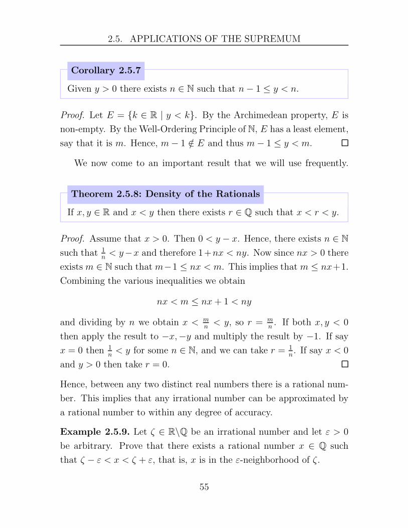
Corollary 2.5.7
Given y > 0 there exists n ∈ N such that n− 1 ≤ y < n.
Proof. Let E = {k ∈ R | y < k}. By the Archimedean property, E is
non-empty. By the Well-Ordering Principle of N, E has a least element,
say that it is m. Hence, m− 1 /∈ E and thus m− 1 ≤ y < m.
We now come to an important result that we will use frequently.
Theorem 2.5.8: Density of the Rationals
If x, y ∈ R and x < y then there exists r ∈ Q such that x < r < y.
Proof. Assume that x > 0. Then 0 < y − x. Hence, there exists n ∈ N
such that 1n < y−x and therefore 1+nx < ny. Now since nx > 0 there
exists m ∈ N such thatm−1 ≤ nx < m. This implies that m ≤ nx+1.
Combining the various inequalities we obtain
nx < m ≤ nx+ 1 < ny
and dividing by n we obtain x < mn < y, so r = m
n . If both x, y < 0
then apply the result to −x,−y and multiply the result by −1. If say
x = 0 then 1n < y for some n ∈ N, and we can take r = 1
n . If say x < 0
and y > 0 then take r = 0.
Hence, between any two distinct real numbers there is a rational num-
ber. This implies that any irrational number can be approximated by
a rational number to within any degree of accuracy.
Example 2.5.9. Let ζ ∈ R\Q be an irrational number and let ε > 0
be arbitrary. Prove that there exists a rational number x ∈ Q such
that ζ − ε < x < ζ + ε, that is, x is in the ε-neighborhood of ζ.
55

2.5. APPLICATIONS OF THE SUPREMUM
Corollary 2.5.10: Density of the Irrationals
If x, y ∈ R and x < y then there exists ξ ∈ R\Q such that x < ξ < y.
Proof. We have that√2x <
√2y. By the Density Theorem,
√2x <
r <√2y for some r ∈ Q. Then ξ = r/
√2.
56

2.5. APPLICATIONS OF THE SUPREMUM
Exercises
Exercise 2.5.1. Let D ⊂ R be non-empty and let f, g : D → R be
functions. Let f + g denote the function defined by
(f + g)(x) = f(x) + g(x)
for any x ∈ D. If f(D) and g(D) are bounded above prove that (f +
g)(D) is also bounded above and that
sup(f + g)(D) ≤ sup f(D) + sup g(D)
Exercise 2.5.2. If y > 0 prove that there exists n ∈ N such that12n < y. (Note: If you begin with 1
2n< y and solve for n then you are assuming
that such an n exists. You are not asked to find an n, you are asked to prove that
such an n exists.)
57

2.6. NESTED INTERVAL THEOREM
2.6 Nested Interval Theorem
If a, b ∈ R and a < b define
(a, b) := {x ∈ R | a < x < b}.
The set (a, b) is called an open interval from a to b. Define also
[a, b] := {x ∈ R | a ≤ x ≤ b}
which we call the closed interval from a to b. The following are called
half-open (or half-closed) intervals:
[a, b) := {x ∈ R | a ≤ x < b}
(a, b] := {x ∈ R | a < x ≤ b}.
If a = b then (a, a) = ∅ and [a, a] = {a}. Infinite intervals are
(a,∞) = {x ∈ R | x > a}(−∞, b) = {x ∈ R | x < b}[a,∞) = {x ∈ R | x ≥ a}
(−∞, b] = {x ∈ R | x ≤ b}.
Below is a characterization of intervals, we will omit the proof.
Theorem 2.6.1
Let S ⊂ R contain at least two points. Suppose that if x, y ∈ S and
x < y then [x, y] ⊂ S. Then S is an interval.
A sequence I1, I2, I3, I4, . . . of intervals is nested if
I1 ⊇ I2 ⊇ I3 ⊇ I4 ⊇ · · ·
58

2.6. NESTED INTERVAL THEOREM
As an example, consider In = [0, 1n] where n ∈ N. Then I1, I2, I3, . . . is
nested:
[0, 1] ⊇ [0, 12] ⊇ [0, 1
3] ⊇ [0, 1
4] · · ·
Notice that since 0 ∈ In for each n ∈ N then
0 ∈∞⋂
n=1
In.
Is there another point in⋂∞
n=1 In? Suppose that x 6= 0 and x ∈ ⋂∞n=1 In.
Then necessarily x > 0. Then there exists m ∈ N such that 1m< x.
Thus, x /∈ [0, 1m ] and therefore x /∈ ⋂∞
n=1 In. Therefore,
∞⋂
n=1
In = {0}.
In general, we have the following.
Theorem 2.6.2: Nested Interval Property
Let I1, I2, I3, . . . be a sequence of nested closed bounded intervals.
Then there exists ξ ∈ R such that ξ ∈ In for all n ∈ N, that
is, ξ ∈ ⋂∞n=1 In. In particular, if In = [an, bn] for n ∈ N, and
a = sup{a1, a2, a3, . . .} and b = inf{b1, b2, b3, . . .} then
{a, b} ⊂∞⋂
n=1
In.
Proof. Since In is a closed interval, we can write In = [an, bn] for some
an, bn ∈ R and an ≤ bn for all n ∈ N. The nested property can be
written as
[a1, b1] ⊇ [a2, b2] ⊇ [a3, b3] ⊇ [a4, b4] ⊇ · · ·Since [an, bn] ⊆ [a1, b1] for all n ∈ N then an ≤ b1 for all n ∈ N.
Therefore, the set S = {an | n ∈ N} is bounded above. Let ξ = sup(S)
59

2.6. NESTED INTERVAL THEOREM
and thus an ≤ ξ for all n ∈ N. We will show that ξ ≤ bn for all n ∈ N
also. Let n ∈ N be arbitrary. If k ≤ n then [an, bn] ⊆ [ak, bk] and
therefore ak ≤ an ≤ bn. On the other hand, if n < k then [ak, bk] ⊂[an, bn] and therefore an ≤ ak ≤ bn. In any case, ak ≤ bn for all
k ∈ N. Hence, bn is an upper bound of S, and thus ξ ≤ bn. Since
n ∈ N was arbitrary, we have that ξ ≤ bn for all n ∈ N. Therefore,
an ≤ ξ ≤ bn for all n ∈ N, that is ξ ∈ ⋂∞n=1[an, bn]. The proof that
inf{b1, b2, b3, . . .} ∈ ⋂∞n=1 In is similar.
The following theorem gives a condition when⋂∞
n=1 In contains a single
point.
Theorem 2.6.3
Let In = [an, bn] be a sequence of nested closed bounded intervals.
If
inf{bn − an | n ∈ N} = 0
then⋂n
n=1 In is a singleton set.
Example 2.6.4. Let In =[1− 1
n, 1 +1n
]for n ∈ N.
(a) Prove that I1, I2, I3, . . . is a sequence of nested intervals.
(b) Find⋂∞
n=1 In.
Using the Nested Interval property of R, we give another proof that
R is uncountable
Theorem 2.6.5: Reals Uncountable
The real numbers R are uncountable.
Proof. We will prove that the interval [0, 1] is uncountable. Suppose by
contradiction that I = [0, 1] is countable, and let I = {x1, x2, x3, . . . , }
60

2.6. NESTED INTERVAL THEOREM
be an enumeration of I (formally this means we have a bijection f :
N → [0, 1] and f(n) = xn). Since x1 ∈ I = [0, 1], there exists a closed
and bounded interval I1 ⊂ [0, 1] such that x1 /∈ I1. Next, consider x2.
There exists a closed and bounded interval I2 ⊂ I1 such that x2 /∈ I2.
Next, consider x3. There exists a closed and bounded interval I3 ⊂ I2
such that x3 /∈ I3. By induction, there exists a sequence I1, I2, I3, . . . of
closed and bounded intervals such that xn /∈ In for all n ∈ N. Moreover,
by construction the sequence In is nested and therefore⋂∞
n=1 In is non-
empty, say it contains ξ. Clearly, since ξ ∈ In ⊂ [0, 1] for all n ∈ N
then ξ ∈ [0, 1]. Now, since xn /∈ In for each n ∈ N then xn /∈ ⋂∞n=1 In.
Therefore, ξ 6= xn for all n ∈ N and thus ξ /∈ I = {x1, x2, . . .} = [0, 1],
which is a contradiction since ξ ∈ [0, 1]. Therefore, [0, 1] is uncountable
and this implies that R is also uncountable.
61

2.6. NESTED INTERVAL THEOREM
Exercises
Exercise 2.6.1. Let In =[0, 1n]for n ∈ N. Prove that
⋂∞n=1 In = {0}.
62

3
Sequences
In the tool box used to build analysis, if the Completeness property of
the real numbers is the hammer then sequences are the nails. Almost
everything that can be said in analysis can be, and is, done using se-
quences. For this reason, the study of sequences will occupy us for the
next foreseeable future.
3.1 Limits of Sequences
A sequence of real numbers is a function X : N → R. Informally,
the sequence X can be written as an infinite list of real numbers as
X = (x1, x2, x3, . . .), where xn = X(n). Other notations for sequences
are (xn) or {xn}∞n=1; we will use (xn).
Some sequences can be written explicitly with a formula such as
xn = 1n , xn = 1
2n , or
xn = (−1)n cos(n2 + 1),
or we could be given the first few terms of the sequence, such as
X = (3, 3.1, 3.14, 3.141, 3.1415, . . .).
63

3.1. LIMITS OF SEQUENCES
Some sequences may be given recursively. For example,
x1 = 1, xn+1 =xnn+ 1
, n ≥ 1.
Using the definition of xn+1 and the initial value x1 we can in principle
find all the terms:
x2 =1
2, x3 =
1/2
3, x4 =
1/6
4, . . .
A famous sequence given recursively is the Fibonacci sequence which
is defined as x1 = 1, x2 = 1, and
xn+1 = xn−1 + xn, n ≥ 2.
Then
x3 = 2, x4 = 3, x5 = 5, . . .
The range of a sequence (xn) is the set
{xn | n ∈ N},
that is, the usual range of a function. However, the range of a sequence
is not the actual sequence (the range is a set and a sequence is a func-
tion). For example, if X = (1, 2, 3, 1, 2, 3, . . .) then the range of X is
{1, 2, 3}. If xn = sin(nπ2 ) then the range of (xn) is {1, 0,−1}.Many concepts in analysis can be described using the long-term or
limiting behavior of sequences. In calculus, you undoubtedly developed
techniques to compute the limit of basic sequences (and hence show
convergence) but you might have omitted the rigorous definition of the
convergence of a sequence. Perhaps you were told that a given sequence
(xn) converges to L if as n→ ∞ the values xn get closer to L. Although
this is intuitively sound, we need a more precise way to describe the
meaning of the convergence of a sequence. Before we give the precise
definition, we will consider an example.
64

3.1. LIMITS OF SEQUENCES
Example 3.1.1. Consider the sequence (xn) whose nth term is given
by xn = 3n+2n+1 . The values of (xn) for several values of n are displayed
in Table 3.1.
n xn1 2.500000002 2.666666673 2.750000004 2.800000005 2.8333333350 2.98039216101 2.99019608
10,000 2.999900011,000,000 2.999999002,000,000 2.99999950
Table 3.1: Values of the sequence xn = 3n+2n+1
The above data suggests that the values of the sequence (xn) become
closer and closer to the number L = 3. For example, suppose that
ε = 0.005 and consider the ε-neighborhood of L = 3, that is, the
interval (3−ε, 3+ε) = (2.995, 3.005). Not all the terms of the sequence
(xn) are in the ε-neighborhood, however, it seems that all the terms of
the sequence from x101 and onward are inside the ε-neighborhood. In
other words, IF n ≥ 101 then 3 − ε < xn < 3 + ε, or equivalently
|xn − 3| < ε. Suppose now that ε = 0.00001 and thus the new ε-
neighborhood is (3−ε, 3+ε) = (2.99999, 3.000001). Then it is no longer
true that |xn − 3| < ε for all n ≥ 101. However, it seems that all the
terms of the sequence from x1000000 and onward are inside the smaller
ε-neighborhood, in other words, |xn − 3| < ε for all n ≥ 1, 000, 000.
We can extrapolate these findings and make the following hypothesis:
For any given ε > 0 there exists a natural number K ∈ N such that if
n ≥ K then |xn − L| < ε.
65
3.1. LIMITS OF SEQUENCES
The above example and our analysis motivates the following defini-
tion.
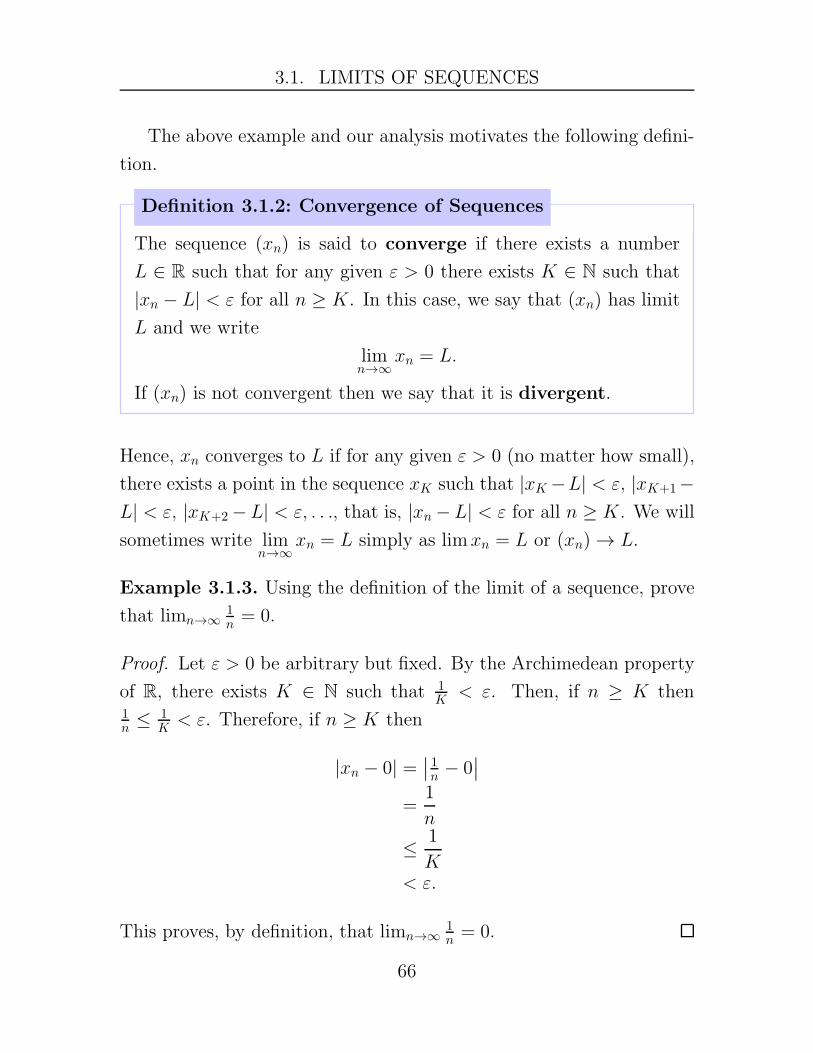
Definition 3.1.2: Convergence of Sequences
The sequence (xn) is said to converge if there exists a number
L ∈ R such that for any given ε > 0 there exists K ∈ N such that
|xn − L| < ε for all n ≥ K. In this case, we say that (xn) has limit
L and we write
limn→∞
xn = L.
If (xn) is not convergent then we say that it is divergent.
Hence, xn converges to L if for any given ε > 0 (no matter how small),
there exists a point in the sequence xK such that |xK −L| < ε, |xK+1−L| < ε, |xK+2 −L| < ε, . . ., that is, |xn −L| < ε for all n ≥ K. We will
sometimes write limn→∞
xn = L simply as limxn = L or (xn) → L.
Example 3.1.3. Using the definition of the limit of a sequence, prove
that limn→∞1n= 0.
Proof. Let ε > 0 be arbitrary but fixed. By the Archimedean property
of R, there exists K ∈ N such that 1K < ε. Then, if n ≥ K then
1n ≤ 1
K < ε. Therefore, if n ≥ K then
|xn − 0| =∣∣ 1n− 0∣∣
=1
n
≤ 1
K< ε.
This proves, by definition, that limn→∞1n = 0.
66

3.1. LIMITS OF SEQUENCES
Example 3.1.4. Using the definition of the limit of a sequence, prove
that limn→∞3n+2n+1 = 3.
Proof. Given an arbitrary ε > 0, we want to prove that there exists
K ∈ N such that∣∣∣∣
3n+ 2
n+ 1− 3
∣∣∣∣< ε, ∀ n ≥ K.
Start by analyzing |xn − L|:
|xn − L| =∣∣∣∣
3n+ 2
n+ 1− 3
∣∣∣∣
=
∣∣∣∣
−1
n+ 1
∣∣∣∣
=1
n+ 1.
Now, the condition that∣∣∣∣
3n+ 2
n+ 1− 3
∣∣∣∣=
1
n+ 1< ε
it is equivalent to1
ε− 1 < n.
Now let’s write the formal proof.
Let ε > 0 be arbitrary and let K ∈ N be such that 1ε− 1 < K.
Then, 1K+1 < ε. Now if n ≥ K then 1
n+1 ≤ 1K+1 and thus if n ≥ K then
∣∣∣∣
3n+ 2
n+ 1− 3
∣∣∣∣=
∣∣∣∣
−1
n+ 1
∣∣∣∣
=1
n+ 1
≤ 1
K + 1< ε.
By definition, this proves that (xn) → 3.
67
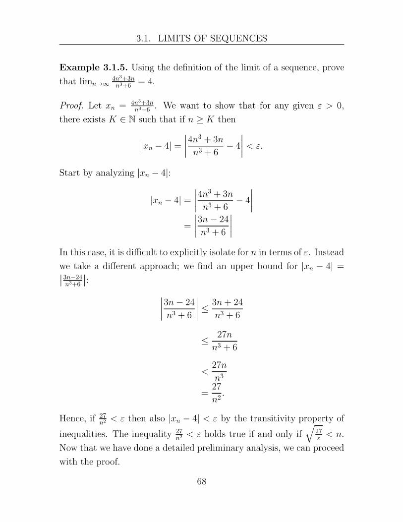
3.1. LIMITS OF SEQUENCES
Example 3.1.5. Using the definition of the limit of a sequence, prove
that limn→∞4n3+3nn3+6 = 4.
Proof. Let xn = 4n3+3nn3+6 . We want to show that for any given ε > 0,
there exists K ∈ N such that if n ≥ K then
|xn − 4| =∣∣∣∣
4n3 + 3n
n3 + 6− 4
∣∣∣∣< ε.
Start by analyzing |xn − 4|:
|xn − 4| =∣∣∣∣
4n3 + 3n
n3 + 6− 4
∣∣∣∣
=
∣∣∣∣
3n− 24
n3 + 6
∣∣∣∣
In this case, it is difficult to explicitly isolate for n in terms of ε. Instead
we take a different approach; we find an upper bound for |xn − 4| =∣∣3n−24n3+6
∣∣:
∣∣∣∣
3n− 24
n3 + 6
∣∣∣∣≤ 3n+ 24
n3 + 6
≤ 27n
n3 + 6
<27n
n3
=27
n2.
Hence, if 27n2 < ε then also |xn − 4| < ε by the transitivity property of
inequalities. The inequality 27n2 < ε holds true if and only if
√27ε < n.
Now that we have done a detailed preliminary analysis, we can proceed
with the proof.
68
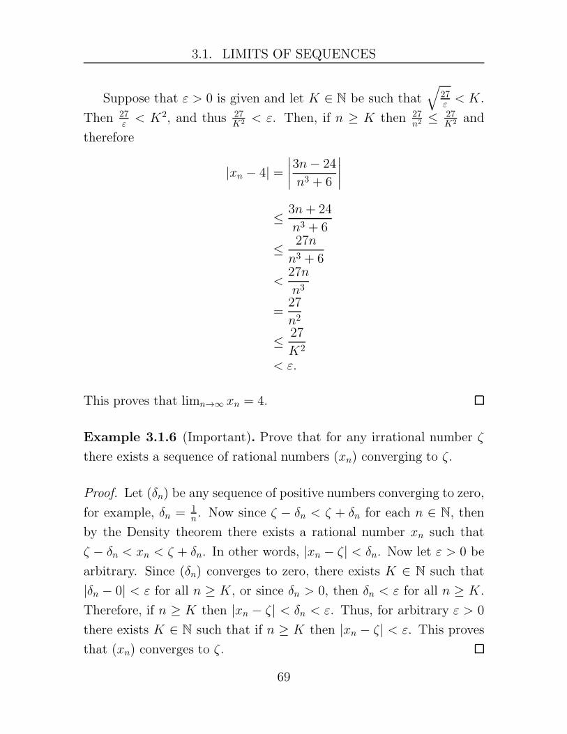
3.1. LIMITS OF SEQUENCES
Suppose that ε > 0 is given and let K ∈ N be such that√
27ε< K.
Then 27ε < K2, and thus 27
K2 < ε. Then, if n ≥ K then 27n2 ≤ 27
K2 and
therefore
|xn − 4| =∣∣∣∣
3n− 24
n3 + 6
∣∣∣∣
≤ 3n+ 24
n3 + 6
≤ 27n
n3 + 6
<27n
n3
=27
n2
≤ 27
K2
< ε.
This proves that limn→∞ xn = 4.
Example 3.1.6 (Important). Prove that for any irrational number ζ
there exists a sequence of rational numbers (xn) converging to ζ.
Proof. Let (δn) be any sequence of positive numbers converging to zero,
for example, δn = 1n . Now since ζ − δn < ζ + δn for each n ∈ N, then
by the Density theorem there exists a rational number xn such that
ζ − δn < xn < ζ + δn. In other words, |xn − ζ| < δn. Now let ε > 0 be
arbitrary. Since (δn) converges to zero, there exists K ∈ N such that
|δn − 0| < ε for all n ≥ K, or since δn > 0, then δn < ε for all n ≥ K.
Therefore, if n ≥ K then |xn − ζ| < δn < ε. Thus, for arbitrary ε > 0
there exists K ∈ N such that if n ≥ K then |xn − ζ| < ε. This proves
that (xn) converges to ζ.
69
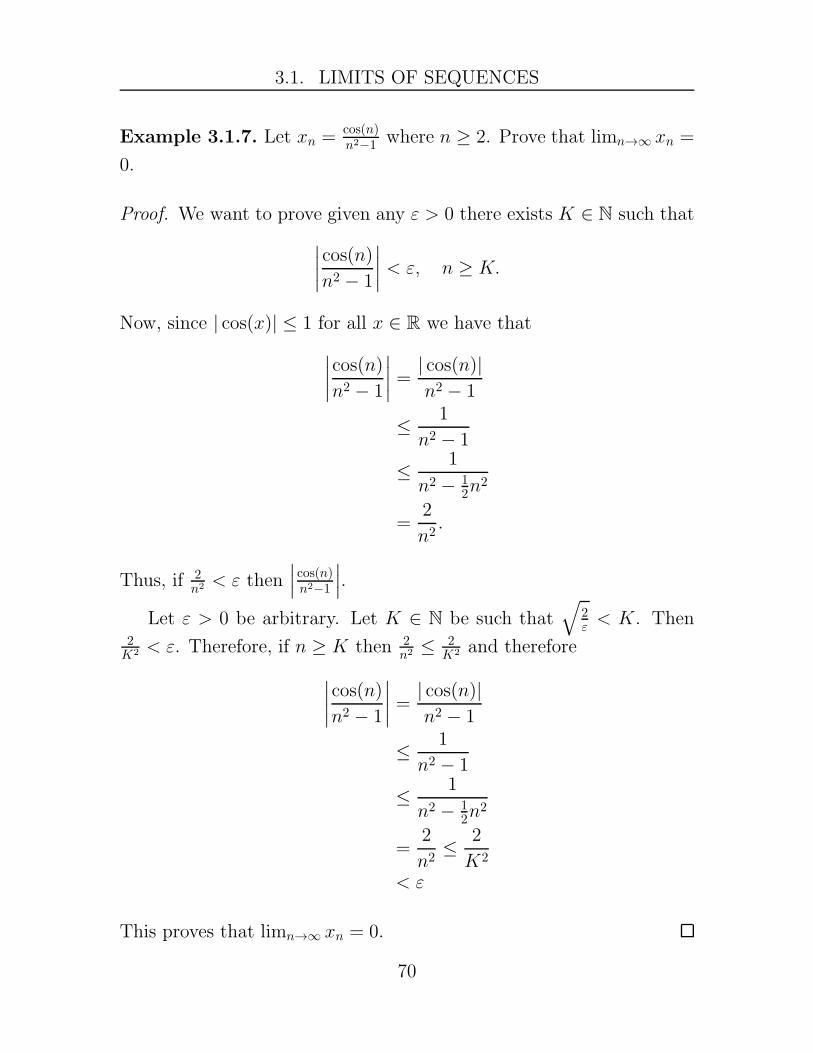
3.1. LIMITS OF SEQUENCES
Example 3.1.7. Let xn = cos(n)n2−1 where n ≥ 2. Prove that limn→∞ xn =
0.
Proof. We want to prove given any ε > 0 there exists K ∈ N such that
∣∣∣∣
cos(n)
n2 − 1
∣∣∣∣< ε, n ≥ K.
Now, since | cos(x)| ≤ 1 for all x ∈ R we have that
∣∣∣∣
cos(n)
n2 − 1
∣∣∣∣=
| cos(n)|n2 − 1
≤ 1
n2 − 1
≤ 1
n2 − 12n
2
=2
n2.
Thus, if 2n2 < ε then
∣∣∣cos(n)n2−1
∣∣∣.
Let ε > 0 be arbitrary. Let K ∈ N be such that√
2ε< K. Then
2K2 < ε. Therefore, if n ≥ K then 2
n2 ≤ 2K2 and therefore
∣∣∣∣
cos(n)
n2 − 1
∣∣∣∣=
| cos(n)|n2 − 1
≤ 1
n2 − 1
≤ 1
n2 − 12n
2
=2
n2≤ 2
K2
< ε
This proves that limn→∞ xn = 0.
70

3.1. LIMITS OF SEQUENCES
Example 3.1.8. Does the sequence (xn) defined by xn = (−1)nnn+1 con-
verge? We will be able to give a definitive answer once we discuss
subsequences.
A useful tool for proving convergence is the following.
Theorem 3.1.9
Let (xn) be a sequence and let L ∈ R. Let (an) be a sequence of
positive numbers such that limn→∞
an = 0. Suppose that there exists
M ∈ N such that
|xn − L| ≤ an, ∀ n ≥M.
Then limn→∞
xn = L.
Proof. Let ε > 0 be arbitrary. Since an → 0, there exists K1 ∈ N such
that an < ε for all n ≥ K1. Let K = max{M,K1}. Then if n ≥ K
then an < ε and |xn − L| ≤ an. Thus if n ≥ K then
|xn − L| ≤ an < ε.
Example 3.1.10. Suppose that 0 < r < 1. Prove that limn→∞ rn = 0.
Proof. We first note that
r =11r
=1
1 + x
where x = 1r − 1 and since r < 1 then x > 0. Now, by Bernoulli’s
71

3.1. LIMITS OF SEQUENCES
inequality it holds that (1 + x)n ≥ 1 + xn for all n ∈ N and therefore
rn =1
(1 + x)n
≤ 1
1 + nx
<1
nx.
Now since limn→∞1nx = 0 it follows that limn→∞ rn = 0.
Example 3.1.11. Let xn = n2−12n2+3
. Prove that limn→∞ xn = 12.
Proof. We have that
∣∣∣∣
n2 − 1
2n2 + 3− 1
2
∣∣∣∣=
5
2
1
(2n2 + 3)
<5/2
2n2.
Using the definition of the limit of a sequence, one can show that
limn→∞5
4n2 = 0 and therefore limn→∞ xn = 12 .
Notice that in the definition of the limit of a sequence, we wrote
“there exists a number L”. Could there be more than one number L
satisfying the definition? Before we go any further, we prove that if a
sequence converges then it has a unique limit.
Theorem 3.1.12: Uniqueness of Limits
A convergent sequence can have at most one limit.
Proof. Suppose that (xn) → L1 and that (xn) → L2. Let ε > 0 be
arbitrary. Then there exists K1 such that |xn − L1| < ε/2 for all
n ≥ K1 and there exists K2 such that |xn − L2| < ε/2 for all n ≥ K2.
72

3.1. LIMITS OF SEQUENCES
Let K = max{K1, K2}. Then for n ≥ K it holds that |xn − L1| < ε/2
and also |xn − L2| < ε/2 and therefore
|L1 − L2| = |L1 − xn + xn − L2|< |xn − L1|+ |xn − L2|< ε/2 + ε/2
= ε.
Hence, |L1 −L2| < ε for all ε > 0, and therefore by Theoreom 2.2.7 we
conclude that |L1 − L2| = 0, that is, L1 − L2 = 0.
The ultimate long-time behavior of a sequence will not change if
we discard a finite number of terms of the sequence. To be pre-
cise, suppose that X = (x1, x2, x3, . . .) is a sequence and let Y =
(xm+1, xm+2, xm+3, . . .), that is, Y is the sequence obtained from X by
discarding the firstm terms of X. In this case, we will call Y them-tail
of X. The next theorem states, not surprisingly, that the convergence
properties of X and Y are the same.
Theorem 3.1.13: Tails of Sequences
Let X : N → R be a sequence and let Y : N → R be the sequence
obtained from X by discarding the first m ∈ N terms of X, in other
words, Y (n) = X(m+ n). Then X converges to L if and only if Y
converges to L.
73

3.1. LIMITS OF SEQUENCES
Exercises
Exercise 3.1.1. Write the first three terms of the recursively defined
sequence x1 = 1, xn+1 =12(xn +
2xn) for n ≥ 1.
Exercise 3.1.2. Use the definition of the limit of a sequence to establish
the following limits:
(a) limn→∞
n+ 1
3n=
1
3
(b) limn→∞
3n2 + 2
4n2 + 1=
3
4
(c) limn→∞
(−1)nn
n2 + 1= 0
Exercise 3.1.3. Prove that limn→∞ |xn| = 0 if and only if limn→∞ xn =
0.
Exercise 3.1.4. Suppose that S ⊂ R is non-empty and bounded above
and let u = supS. Show that there exists a sequence (xn) such that
xn ∈ S for all n ∈ N and limn→∞ xn = u. Hint: If ε > 0 then clearly
u−ε < u. Since u = sup(S) there exists x ∈ S such that u−ε < x < u.
Hence, for each ε > 0 there exists x ∈ S such that |x− u| < ε.
74

3.2. LIMIT THEOREMS
3.2 Limit Theorems
Proving that a particular number L ∈ R is the limit of a given sequence
is usually not easy because there is no systematic way to determine
a candidate limit L for a given arbitrary sequence. Instead, we are
frequently interested in just knowing if a given sequence converges or
not, and not so much on finding the actual limit. The theorems in this
section help us do just that. We begin with a definition.
Definition 3.2.1: Boundedness
A sequence (xn) is said to be bounded if there exists R ≥ 0 such
that |xn| ≤ R for all n ∈ N.
Example 3.2.2. Prove that (xn) is bounded if and only if there exists
numbers R1 and R2 such that R1 ≤ xn ≤ R2 for all n ∈ N.
Theorem 3.2.3: Convergence implies Boundedness
If (xn) is convergent then it is bounded.
Proof. Suppose that (xn) converges to L and let ε > 0 be arbitrary.
There exists K ∈ N such that L − ε < xn < L + ε for all n ≥ K. Let
R1 = inf{x1, x2, . . . , xK−1, L−ε} and R2 = sup{x1, x2, . . . , xK−1, L+ε}.Then R1 ≤ xn ≤ R2 for all n = 1, 2, . . . , K − 1. But also R1 ≤ L− ε <
xn < L+ ε ≤ R2 for all n ≥ K. Hence, R1 ≤ xn ≤ R2 for all n ≥ 1 and
this proves that (xn) is bounded.
Theorem 3.2.4: Convergence under Absolute Value
If (xn) → L then (|xn|) → |L|.
75

3.2. LIMIT THEOREMS
Proof. Follows by the inequality ||xn| − |L|| ≤ |xn − L| (see Corol-
lary 2.3.6). Indeed, for any given ε > 0 there exists K ∈ N such that
|xn − L| < ε for all n ≥ K and therefore ||xn| − |L|| ≤ |xn − L| < ε for
all n ≥ K.
The following theorem describes how the basic operations of arith-
metic preserve convergence.
Theorem 3.2.5: Limit Laws
Suppose that (xn) → L and (yn) →M .
(a) Then (xn + yn) → L+M and (xn − yn) → L−M .
(b) Then (xnyn) → LM .
(c) If yn 6= 0 and M 6= 0 then(xn
yn
)
→ LM .
Proof. (i) By the triangle inequality
|xn + yn − (L+M)| = |xn − L+ yn −M |< |xn − L|+ |yn −M |.
Let ε > 0. There exists K1 such that |xn − L| < ε/2 for n ≥ K1
and there exists K2 such that |yn −M | < ε/2 for n ≥ K2. Let K =
max{K1, K2}. Then for n ≥ K
|xn + yn − (L+M)| < |xn − L|+ |yn −M |< ε/2 + ε/2
= ε.
The proof for (xn − yn) → L−M is similar.
76
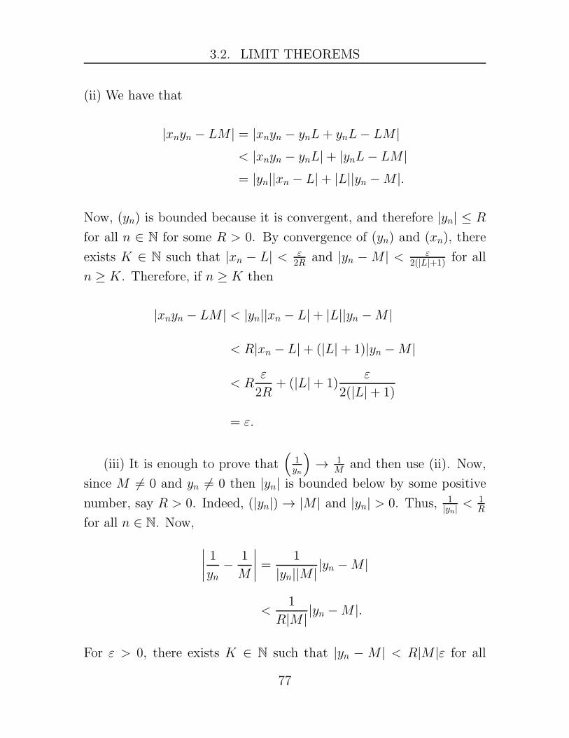
3.2. LIMIT THEOREMS
(ii) We have that
|xnyn − LM | = |xnyn − ynL+ ynL− LM |< |xnyn − ynL|+ |ynL− LM |= |yn||xn − L|+ |L||yn −M |.
Now, (yn) is bounded because it is convergent, and therefore |yn| ≤ R
for all n ∈ N for some R > 0. By convergence of (yn) and (xn), there
exists K ∈ N such that |xn − L| < ε2R and |yn −M | < ε
2(|L|+1) for all
n ≥ K. Therefore, if n ≥ K then
|xnyn − LM | < |yn||xn − L|+ |L||yn −M |
< R|xn − L|+ (|L|+ 1)|yn −M |
< Rε
2R+ (|L|+ 1)
ε
2(|L|+ 1)
= ε.
(iii) It is enough to prove that(
1yn
)
→ 1M and then use (ii). Now,
since M 6= 0 and yn 6= 0 then |yn| is bounded below by some positive
number, say R > 0. Indeed, (|yn|) → |M | and |yn| > 0. Thus, 1|yn| <
1R
for all n ∈ N. Now,
∣∣∣∣
1
yn− 1
M
∣∣∣∣=
1
|yn||M | |yn −M |
<1
R|M | |yn −M |.
For ε > 0, there exists K ∈ N such that |yn − M | < R|M |ε for all
77

3.2. LIMIT THEOREMS
n ≥ K. Therefore, for n ≥ K we have that∣∣∣∣
1
yn− 1
M
∣∣∣∣<
1
R|M | |yn −M |
<1
R|M |R|M |ε
= ε.
Corollary 3.2.6
Suppose that (xn) → L. Then (xkn) → Lk for any k ∈ N.
The next theorem states that the limit of a convergent sequence of
non-negative terms is non-negative.
Theorem 3.2.7
Suppose that (xn) → L. If xn ≥ 0 for all n ∈ N then L ≥ 0.
Proof. We prove the contrapositive, that is, we prove that if L < 0 then
there exists K ∈ N such that xK < 0. Suppose then that L < 0. Let
ε > 0 be such that L+ ε < 0. Since (xn) → L, there exists K ∈ N such
that xK < L+ ε, and thus by transitivity we have xK < 0.
Corollary 3.2.8: Comparison
Suppose that (xn) and (yn) are convergent and suppose that there
exists M ∈ N such that xn ≤ yn for all n ≥ M . Then limn→∞
xn ≤limn→∞
yn.
78

3.2. LIMIT THEOREMS
Proof. Suppose for now that M = 1, that is, xn ≤ yn for all n ∈ N.
Consider the sequence zn = yn − xn. Then zn ≥ 0 for all n ∈ N and
(zn) is convergent since it is the difference of convergent sequences. By
Theorem 3.2.7, we conclude that limn→∞ zn ≥ 0. But
limn→∞
zn = limn→∞
(yn − xn)
= limn→∞
yn − limn→∞
xn
and therefore limn→∞ yn−limn→∞ xn ≥ 0, which is the same as limn→∞ yn ≥limn→∞ xn. If M > 1, then we can apply the theorem to the M -tail of
the sequences of (xn) and (yn) and the result follows.
Corollary 3.2.9
Suppose that a ≤ xn ≤ b and limn→∞
xn = L. Then a ≤ L ≤ b.
Proof. We have that 0 ≤ xn − a ≤ b − a. The sequence yn = b − a is
constant and converges to b − a. The sequence zn = xn − a converges
to L − a. Therefore, by the previous theorem, 0 ≤ L − a ≤ b − a, or
a ≤ L ≤ b.
Theorem 3.2.10: Squeeze Theorem
Suppose that yn ≤ xn ≤ zn for all n ∈ N. Assume that (yn) → L
and also (zn) → L. Then (xn) is convergent and (xn) → L.
Proof. Let ε > 0 be arbitrary. There exists K1 ∈ N such that L −ε < yn < L + ε for all n ≥ K1 and there exists K2 ∈ N such that
L − ε < zn < L + ε for all n ≥ K2. Let K = max{K1, K2}. Then if
n ≥ K then
L− ε < yn ≤ xn ≤ zn < L+ ε.
79

3.2. LIMIT THEOREMS
Therefore, for n ≥ K we have that
L− ε < xn < L+ ε
and thus limn→∞ xn = L.
Remark 3.2.11. Some people call the Squeeze Theorem the Sandwich
Theorem; we are not those people.
Example 3.2.12. Let 0 < a < b and let xn = (an + bn)1/n. Prove that
limn→∞
xn = b.
Theorem 3.2.13: Ratio Test
Let (xn) be a sequence such that xn > 0 for all n ∈ N and sup-
pose that L = limn→∞
xn+1
xnexists. If L < 1 then (xn) converges and
limn→∞
xn = 0.
Proof. Let r ∈ R be such that L < r < 1 and set ε = r − L. There
exists K ∈ N such that
xn+1
xn< L+ ε = r
for all n ≥ K. Therefore, for all n ≥ K we have that
0 < xn+1 < rxn.
Thus, xK+1 < rxK , and therefore xK+2 < rxK+1 < r2xK, and induc-
tively for m ≥ 1 it holds that
xK+m < rmxK.
80

3.2. LIMIT THEOREMS
Hence, the tail of the sequence (xn) given by (ym) = (xK+1, xK+2, . . . , )
satisfies
0 < ym < rmxK .
Since 0 < r < 1 it follows that limm→∞ rm = 0 and therefore limm→∞ ym =
0 by the Squeeze theorem. This implies that (xn) converges to 0
also.
81

3.2. LIMIT THEOREMS
Exercises
Exercise 3.2.1. Use the Limit Theorems to prove that if (xn) converges
and (xn + yn) converges then (yn) converges. Give an example of two
sequences (xn) and (yn) such that both (xn) and (yn) diverge but (xn+
yn) converges.
Exercise 3.2.2. Is the sequence yn = (−1)nn4 convergent? Explain.
Exercise 3.2.3. Let (xn) and (yn) be sequences in R. Suppose that
limn→∞ xn = 0 and that (yn) is bounded. Prove that limn→∞ xnyn = 0.
Exercise 3.2.4. Show that if (xn) and (yn) are sequences such that
(xn) and (xn + yn) are convergent, then (yn) is convergent.
Exercise 3.2.5. Give examples of the following:
(a) Divergent sequences (xn) and (yn) such that zn = xnyn converges.
(b) Divergent sequences (xn) and (yn) such that zn = xnyn diverges.
(c) A divergent sequence (xn) and a convergent sequence (yn) such
that zn = xnyn converges.
(d) A divergent sequence (xn) and a convergent sequence (yn) such
that zn = xnyn diverges.
Exercise 3.2.6. Let (xn) and (yn) be sequences and suppose that (xn)
converges to L. Assume that for every ε > 0 there exists M ∈ N such
that |xn − yn| < ε for all n ≥M . Prove that (yn) also converges to L.
Exercise 3.2.7. Let (xn) be a sequence and define a sequence (yn) as
yn =x1 + x2 + · · ·+ xn
n
for n ∈ N. Show that if limn→∞ xn = 0 then limn→∞ yn = 0.
82

3.2. LIMIT THEOREMS
Exercise 3.2.8. Let (xn) be a convergent sequence with limit L. Let
f(x) = a0 + a1x+ · · ·+ akxk be a polynomial. Use the Limit Theorems
to prove that the sequence (yn) defined by yn = f(xn) is convergent
and find the limit of (yn).
Exercise 3.2.9. Apply the Limit Theorems to find the limits of the
following sequences:
(a) xn =
√
2n2 + 3
n2 + 1
(b) xn = (2 + 1/n)2
(c) xn =n+ 1
n√n
(d) xn = 2n/n!
Exercise 3.2.10. Let (xn) be a sequence such that xn 6= 0 for all n ∈ N.
Suppose that limn→∞ xn = L and L > 0. Let w = inf{|xn| : n ∈ N}.Prove that w > 0.
Exercise 3.2.11. Let (xn) be a sequence of positive numbers such that
limn→∞
xn+1
xn= L > 1. Show that (xn) is not bounded and hence is not
convergent.
83

3.3. MONOTONE SEQUENCES
3.3 Monotone Sequences
As we have seen, a convergent sequence is necessarily bounded, and it
is straightforward to construct examples of sequences that are bounded
but not convergent, for example, (xn) = (1, 0, 1, 0, 1, 0, . . .). In this
section, we prove the Monotone Convergence Theorem which says that
a bounded sequence whose terms increase (or decrease) must necessarily
converge.
Definition 3.3.1: Monotone Sequences
Let (xn) be a sequence.
(i) We say that (xn) is increasing if xn ≤ xn+1 for all n ∈ N.
(ii) We say that (xn) is decreasing if xn+1 ≤ xn for all n ∈ N.
(iii) We say that (xn) is monotone if it is either increasing or
decreasing.
Example 3.3.2. Prove that if (xn) is increasing then (xn) is bounded
below. Similarly, prove that if (xn) is decreasing then (xn) is bounded
above.
84

3.3. MONOTONE SEQUENCES
Theorem 3.3.3: Monotone Convergence Theorem
If (xn) is bounded and monotone then (xn) is convergent. In par-
ticular:
(i) if (xn) is bounded above and increasing then
limn→∞
xn = sup{xn : n ∈ N},
(ii) if (xn) is bounded below and decreasing then
limn→∞
xn = inf{xn : n ∈ N}.
Proof. Suppose that (xn) is bounded above and increasing. Let u =
sup{xn | n ∈ N} and let ε > 0 be arbitrary. Then by the properties of
the supremum, there exists xK such that u − ε < xK ≤ u. Since (xn)
is increasing, and u is an upper bound for the range of the sequence, it
follows that xK ≤ xn ≤ u for all n ≥ K. Therefore, u− ε < xn ≤ u for
all n ≥ K. Clearly, this implies that u− ε < xn < u+ ε for all n ≥ K.
Since ε > 0 was arbitrary, this proves that (xn) converges to u.
Suppose now that (xn) is bounded below and decreasing. Let w =
inf{xn | n ∈ N} and let ε > 0 be arbitrary. Then by the properties of
the infimum, there exists xK such that w ≤ xK < w + ε. Since (xn)
is decreasing, and w is a lower bound for the range of the sequence, it
follows that w ≤ xn ≤ xK for all n ≥ K. Therefore, w ≤ xn < w + ε
for all n ≥ K. Hence, w − ε < xn < w + ε for all n ≥ K. Since ε > 0
was arbitrary, this proves that (xn) converges to w.
The Monotone Convergence Theorem (MCT) is an important tool
in real analysis and we will use it frequently; notice that it is more-
85

3.3. MONOTONE SEQUENCES
or-less a direct consequence of the Completeness Axiom. In fact, we
could have taken as our starting axiom the MCT and then proved the
Completeness property of R.
Example 3.3.4. By the MCT, a bounded sequence that is also mono-
tone is convergent. However, it is easy to construct a convergent se-
quence that is not monotone. Provide such an example.
The MCT can be used to show convergence of recursively defined
sequences. To see how, suppose that (xn) is defined recursively as
x1 = a and
xn+1 = f(xn)
where f is some given function. For example, say x1 = 2 and
xn+1 = 2 +1
xn.
Hence, in this case f(x) = 2 + 1x . If (xn) is bounded and increasing
then by the MCT (xn) converges, but we do not know what the limit
is. However, for example, if f is a polynomial/rational function of x
then we can conclude that L = limn→∞ xn must satisfy the equation
L = f(L).
Indeed, if f is a polynomial/rational function then by the Limit Laws
we have
limn→∞
f(xn) = f( limn→∞
xn) = f(L).
But xn+1 = f(xn) and therefore limn→∞ xn+1 = f(L), which is equiva-
lent to limn→∞ xn = f(L) since (xn+1) is just the 1-tail of the sequence
(xn). Therefore, L = f(L) as claimed. From the equation L = f(L) we
can solve for L if possible.
86

3.3. MONOTONE SEQUENCES
Example 3.3.5. Consider the sequence (xn) defined recursively as x1 =
1 and
xn+1 =12xn +
1
4, ∀ n ≥ 1.
Prove that (xn) converges and find the limit.
Proof. We prove by induction that 12≤ xn for all n ∈ N, that is, (xn) is
bounded below by 12. First of all, it is clear that 1
2 ≤ x1. Now assume
that 12 ≤ xn for some n ∈ N. Then
xn+1 =12xn +
1
4
≥ 1
2· 12+
1
4
=1
2.
Hence, (xn) is bounded below by 12 . We now prove that (xn) is decreas-
ing. We compute that x2 =12+ 1
4= 3
4, and thus x2 < x1. Assume now
that xn < xn−1 for some n ∈ N. Then
xn+1 <1
2xn−1 +
1
4= xn.
Hence, by induction we have shown that (xn) is decreasing. By the
MCT, (xn) is convergent. Suppose that (xn) → L. Then also (xn+1) →L and the sequence yn = 1
2xn + 14 converges to 1
2L + 14. Therefore,
L = 12L+ 1
4 and thus L = 1/2.
Before we embark on the next example, we recall that
1 + r + r2 + · · · + rn−1 =1− rn
1− r
and if 0 < r < 1 then 0 < rn < r < 1 and therefore
1− rn
1− r<
1
1− r.
87
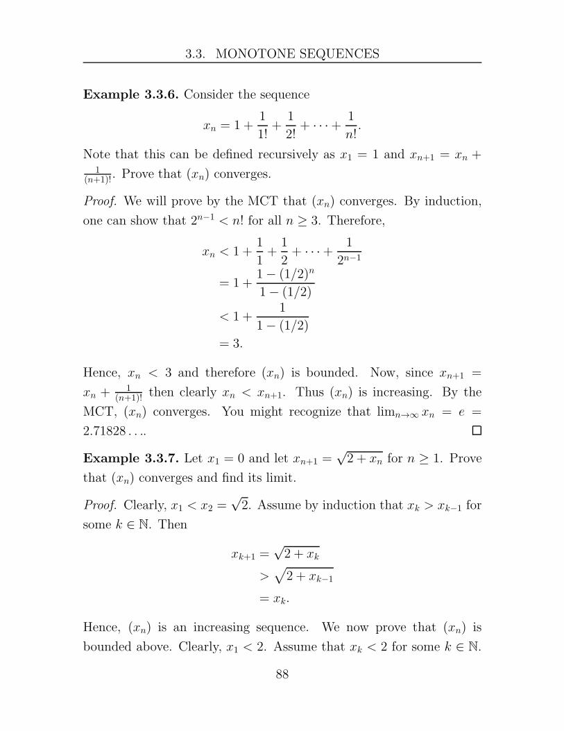
3.3. MONOTONE SEQUENCES
Example 3.3.6. Consider the sequence
xn = 1 +1
1!+
1
2!+ · · ·+ 1
n!.
Note that this can be defined recursively as x1 = 1 and xn+1 = xn +1
(n+1)!. Prove that (xn) converges.
Proof. We will prove by the MCT that (xn) converges. By induction,
one can show that 2n−1 < n! for all n ≥ 3. Therefore,
xn < 1 +1
1+
1
2+ · · ·+ 1
2n−1
= 1 +1− (1/2)n
1− (1/2)
< 1 +1
1− (1/2)
= 3.
Hence, xn < 3 and therefore (xn) is bounded. Now, since xn+1 =
xn + 1(n+1)! then clearly xn < xn+1. Thus (xn) is increasing. By the
MCT, (xn) converges. You might recognize that limn→∞ xn = e =
2.71828 . . ..
Example 3.3.7. Let x1 = 0 and let xn+1 =√2 + xn for n ≥ 1. Prove
that (xn) converges and find its limit.
Proof. Clearly, x1 < x2 =√2. Assume by induction that xk > xk−1 for
some k ∈ N. Then
xk+1 =√2 + xk
>√
2 + xk−1
= xk.
Hence, (xn) is an increasing sequence. We now prove that (xn) is
bounded above. Clearly, x1 < 2. Assume that xk < 2 for some k ∈ N.
88

3.3. MONOTONE SEQUENCES
Then xk+1 =√2 + xk <
√2 + 2 = 2. This proves that (xn) is bounded
above. By the MCT, (xn) converges, say to L. Moreover, since xn ≥ 0
(as can be proved by induction), then L ≥ 0. Therefore, L =√2 + L
and then L2 − L− 2 = 0. Hence, L = 1±√1+82 = 1±3
2 . Since L ≥ 0 then
L = 2.
Example 3.3.8. Consider the sequence xn =(1 + 1
n
)n. We will show
that (xn) is bounded and increasing, and therefore by the MCT (xn)
convergent. The limit of this sequence is the number e. From the
binomial theorem
xn =n∑
k=0
(n
k
)1
nk
= 1 +n
n+
1
2!
n(n− 1)
n2+
1
3!
n(n− 1)(n− 2)
n3+ · · ·
+1
n!
n(n− 1)(n− 2) · · · (n− (n− 1))
nk
= 1 + 1 +1
2!(1− 1
n) +1
3!(1− 1
n)(1− 1n) + · · ·
+1
n!(1− 1
n)(1− 1
n) · · · (1− (n− 1)/n)
< 1 + 1 +1
2!+
1
3!+ · · ·+ 1
n!
< 1 + 1 +1
2+
1
22+ · · ·+ 1
2n−1
= 1 +1− (1/2)n
1− 1/2
< 3
where we used that 2n−1 < n! for all n ≥ 3. This shows that (xn) is
89

3.3. MONOTONE SEQUENCES
bounded. Now, for each 1 ≤ k ≤ n, we have that
(n
k
)1
nk=n(n− 1)(n− 2) · · · (n− (k − 1))
nk
= (1− 1n)(1− 2
n) · · · (1− k−1n ).
And similarly,
(n+ 1
k
)1
(n+ 1)k= (1− 1
n+1)(1− 2n+1) · · · (1− k−1
n+1).
It is clear that (1 − jn) < (1 − j
n+1) for all 1 ≤ j ≤ n. Hence,(nk
)1nk <
(n+1k
)1
(n+1)k. Therefore, xn < xn+1, that is, (xn) is increasing. By the
MCT, (xn) converges to sup{xn : n ∈ N}.
90

3.3. MONOTONE SEQUENCES
Exercises
Exercise 3.3.1. Let (xn) be an increasing sequence, let (yn) be a de-
creasing sequence, and assume that xn ≤ yn for all n ∈ N. Prove that
limn→∞
xn and limn→∞
yn exist, and that limn→∞
xn ≤ limn→∞
yn. Note: Recall that a
sequence (xn) is bounded if there exists a constant R > 0 (independent of n) such
that −R ≤ xn ≤ R for all n ∈ N.
Exercise 3.3.2. Let x1 = 8 and let xn+1 =12xn + 2 for n ≥ 1. Prove
that (xn) is bounded and monotone. Find the limit of (xn).
Exercise 3.3.3. Let x1 = 1 and let xn+1 =n
n+ 1x2n for n ≥ 1. Prove
that (xn) is bounded and monotone. Find the limit of (xn). Hint: Using
induction to prove that (xn) is monotone will not work with this sequence. Instead,
work with xn+1 directly to prove that (xn) is monotone.
Exercise 3.3.4. True or false, a convergent sequence is necessarily
monotone? If it is true, prove it. If it is false, give an example.
91

3.4. BOLZANO-WEIERSTRASS THEOREM
3.4 Bolzano-Weierstrass Theorem
We can gather information about a sequence by studying its subse-
quences. Loosely speaking, a subsequence of (xn) is a new sequence
(yk) such that each term yk is from the original sequence (xn) and the
term yk+1 appears to the “right” of the term yk in the original sequence
(xn). Let us be precise about what we mean to the “right”.
Definition 3.4.1: Subsequences
Let (xn) be a sequence. A subsequence of (xn) is a sequence of
the form (xn1, xn2
, xn3, . . .) where n1 < n2 < n3 < · · · is a sequence
of strictly increasing natural numbers. A subsequence of (xn) will
be denoted by (xnk).
The notation (xnk) of a subsequence indicates that the indexing variable
is k ∈ N. The selection of the elements of (xn) to form a subsequence
(xnk) does not need to follow any particular well-defined pattern but
only that n1 < n2 < n3 < · · · . Notice that for any increasing sequence
n1 < n2 < n3 < · · · of natural numbers, we have
k ≤ nk
for all k ≥ 1.
Example 3.4.2. An example of a subsequence of xn = 1n is the se-
quence (yk) = (1, 13 ,15,
17, . . .). Here we have chosen the odd terms of the
sequence (xn) to create (yk). In other words, if we write that yk = xnk
then nk = 2k − 1. Another example of a subsequence of (xn) is ob-
tained by taking the even terms to get the subsequence (12, 14, 16, . . .), so
that here nk = 2k. In general, we can take any increasing selection
92

3.4. BOLZANO-WEIERSTRASS THEOREM
n1 < n2 < n3 < · · · , such as
( 111, 1303, 12000
, . . .)
to form a subsequence of (xn).
Example 3.4.3. Two subsequences of
(xn) = (1,−1, 12 ,−1, 13 ,−1, 14 ,−1, . . .)
(−1,−1,−1, . . . , ) and (1, 12,13, . . . , ). Both of these subsequences con-
verge to distinct limits.
Example 3.4.4 (Important). We proved thatQ is countable and hence
there is a bijection f : N → Q. The bijection f defines a sequence
(xn) = (x1, x2, x3, x4, . . .)
where xn = f(n). Let L ∈ R be arbitrary. By the density of Q in
R, there exists xn1∈ Q such that xn1
∈ (L − 1, L + 1). Now consider
the interval (L − 12 , L + 1
2). It has infinitely many distinct rational
numbers (by the Density Theorem). Therefore, there exists n2 > n1
such that xn2∈ (L− 1
2 , L + 12). Consider now the interval (L− 1
3 , L +13). It has infinitely many rational numbers, and therefore there exists
n3 > n2 such that xn3∈ (L − 1
3 , L + 13). By induction, there exists
a subsequence (xnk) of (xn) such that |xnk
− L| < 1k for all k ≥ 1.
Therefore, limk→∞ xnk= L. We proved the following: For any real
number L there exists a sequence of rational numbers that converges
to L.
The following theorem is a necessary condition for convergence.
93

3.4. BOLZANO-WEIERSTRASS THEOREM
Theorem 3.4.5
If (xn) → L then every subsequence of (xn) converges to L.
Proof. Let ε > 0. Then there exists K ∈ N such that |xn − L| < ε for
all n ≥ K. Since nK ≥ K and nK < nK+1 < . . ., then |xnk− L| < ε for
all k ≥ K.
The contrapositive of the previous theorem is worth stating.
Theorem 3.4.6
Let (xn) be a sequence.
(i) If (xn) has two subsequences converging to distinct limits then
(xn) is divergent.
(ii) If (xn) has a subsequence that diverges then (xn) diverges.
The following is a very neat result that will supply us with a very
short proof of the main result of this section, namely, the Bolzano-
Weierstrass Theorem.
Theorem 3.4.7
Every sequence has a monotone subsequence.
Proof. Let (xn) be an arbitrary sequence. We will say that the term xm
is a peak if xm ≥ xn for all n ≥ m. In other words, xm is a peak if it is
an upper bound of all the terms coming after it. There are two possible
cases for (xn), either it has an infinite number of peaks or it has a finite
number of peaks. Suppose that it has an infinite number of peaks, say
xm1, xm2
, . . ., and we may assume that m1 < m2 < m3 < · · · . Then,
94
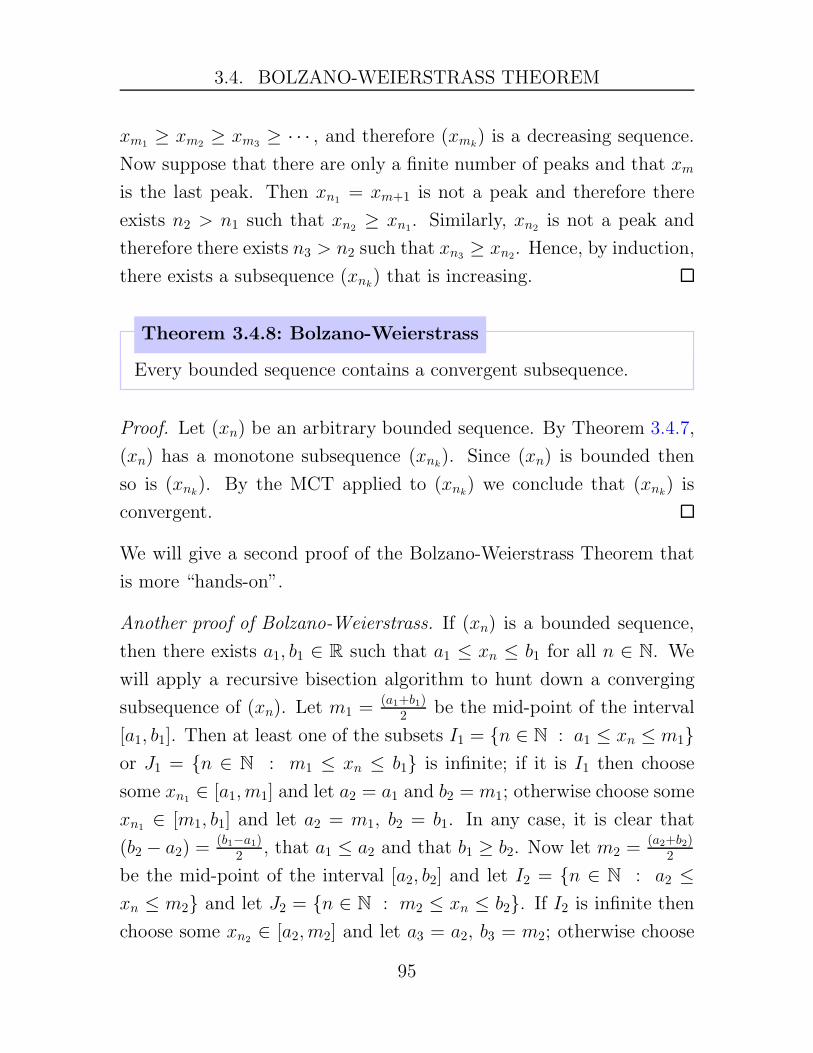
3.4. BOLZANO-WEIERSTRASS THEOREM
xm1≥ xm2
≥ xm3≥ · · · , and therefore (xmk
) is a decreasing sequence.
Now suppose that there are only a finite number of peaks and that xm
is the last peak. Then xn1= xm+1 is not a peak and therefore there
exists n2 > n1 such that xn2≥ xn1
. Similarly, xn2is not a peak and
therefore there exists n3 > n2 such that xn3≥ xn2
. Hence, by induction,
there exists a subsequence (xnk) that is increasing.
Theorem 3.4.8: Bolzano-Weierstrass
Every bounded sequence contains a convergent subsequence.
Proof. Let (xn) be an arbitrary bounded sequence. By Theorem 3.4.7,
(xn) has a monotone subsequence (xnk). Since (xn) is bounded then
so is (xnk). By the MCT applied to (xnk
) we conclude that (xnk) is
convergent.
We will give a second proof of the Bolzano-Weierstrass Theorem that
is more “hands-on”.
Another proof of Bolzano-Weierstrass. If (xn) is a bounded sequence,
then there exists a1, b1 ∈ R such that a1 ≤ xn ≤ b1 for all n ∈ N. We
will apply a recursive bisection algorithm to hunt down a converging
subsequence of (xn). Let m1 =(a1+b1)
2 be the mid-point of the interval
[a1, b1]. Then at least one of the subsets I1 = {n ∈ N : a1 ≤ xn ≤ m1}or J1 = {n ∈ N : m1 ≤ xn ≤ b1} is infinite; if it is I1 then choose
some xn1∈ [a1, m1] and let a2 = a1 and b2 = m1; otherwise choose some
xn1∈ [m1, b1] and let a2 = m1, b2 = b1. In any case, it is clear that
(b2 − a2) =(b1−a1)
2 , that a1 ≤ a2 and that b1 ≥ b2. Now let m2 =(a2+b2)
2
be the mid-point of the interval [a2, b2] and let I2 = {n ∈ N : a2 ≤xn ≤ m2} and let J2 = {n ∈ N : m2 ≤ xn ≤ b2}. If I2 is infinite then
choose some xn2∈ [a2, m2] and let a3 = a2, b3 = m2; otherwise choose
95

3.4. BOLZANO-WEIERSTRASS THEOREM
some xn2∈ [m2, b2] and let a3 = m2 and b3 = b2. In any case, it is
clear that (b3 − a3) =(b1−a1)
22 , that a2 ≤ a3 and b3 ≤ b2. By induction,
there exists sequences (ak), (bk), and (xnk) such that ak ≤ xnk
≤ bk
and (bk − ak) = (b1−a1)2k−1 , (ak) is increasing and (bk) is decreasing. It
is clear that ak ≤ b and a ≤ bk for all k ∈ N. Hence, by the MCT,
(ak) and (bk) are convergent. Moreover, since (bk − ak) =(b1−a1)2k−1 then
lim(bk − ak) = 0 and consequently lim ak = lim bk = L. By the Squeeze
theorem we conclude that limk→∞ xnk= L.
Notice that the proofs of the Bolzano-Weierstrass Theorem rely on
the Monotone Convergence Theorem and the latter relies on the Com-
pleteness Axiom. We therefore have the following chain of implications:
Completeness =⇒ MCT =⇒ Bol-Wei
It turns out that if we had taken as our starting axiom the Bolzano-
Weierstrass theorem then we could prove the Completeness property
and then of course the MCT. In other words, all three statements are
equivalent:
Completeness ⇐⇒ MCT ⇐⇒ Bol-Wei
96

3.4. BOLZANO-WEIERSTRASS THEOREM
Exercises
Exercise 3.4.1. Prove that the following sequences are divergent.
(a) xn = 1− (−1)n + 1/n
(b) xn = sin(nπ/4)
(Hint: Theorem 3.4.6)
Exercise 3.4.2. Suppose that xn ≥ 0 for all n ∈ N and suppose that
limn→∞
(−1)nxn = L exists. Prove that L = 0 and that also limn→∞
xn = L.
(Hint: Consider subsequences of (−1)nxn.)
Exercise 3.4.3. Let (xn) be a sequence.
(a) Suppose that (xn) is increasing. Prove that if (xn) has a sub-
sequence (xnk) that is bounded above then (xn) is also bounded
above.
(b) Suppose that (xn) is decreasing. Prove that if (xn) has a sub-
sequence (xnk) that is bounded below then (xn) is also bounded
below.
Exercise 3.4.4. True or false: If (xn) is bounded and diverges then
(xn) has two subsequences that converge to distinct limits. Explain.
Exercise 3.4.5. Give an example of a sequence (xn) with the following
property: For each number L ∈{1, 12 ,
13 ,
14 , . . .
}there exists a subse-
quence (xnk) such that xnk
→ L. Hint: If you are spending a lot of
time on this question then you have not been reading this textbook
carefully.
97

3.4. BOLZANO-WEIERSTRASS THEOREM
Exercise 3.4.6. Suppose that x1 and y1 satisfy 0 < x1 < y1 and define
xn+1 =√xnyn, yn+1 =
xn + yn2
for n ≥ 1. Prove that (xn) and (yn) are convergent and that limxn =
lim yn. (Hint: First show that√xy ≤ (x+ y)/2 for any x, y > 0.)
Exercise 3.4.7. Let (xn) be a sequence and define the sequence (yn)
as
yn =x1 + x2 + · · ·+ xn
n
Prove that if (xn) → L then (yn) → L.
98

3.5. LIMSUP AND LIMINF
3.5 limsup and liminf
The behavior of a convergent sequence is easy to understand. Indeed,
if (xn) → L then eventually the terms of (xn) will be arbitrarily close to
L for n sufficiently large. What else is there to say? In this section, we
focus on bounded sequences that do not necessarily converge. The idea
is that we would like to develop a limit concept for these sequences,
and in particular, a “limiting upper bound”.
Let (xn) be an arbitrary sequence and introduce the set S defined
as the set of all the limits of convergent subsequences of (xn), that is,
S = {L ∈ R | (xnk) → L} .
We will call S the subsequences limit set of (xn).
Example 3.5.1. If (xn) is bounded and S is the subsequences limit set
of (xn) explain why S is non-empty.
Example 3.5.2. Here are six examples of sequences and the corre-
sponding subsequences limit set. Notice that in the cases where (xn)
(xn) S(1, 12 ,
13, . . .) {0}
(1,−1, 1,−1, . . .) {1,−1}(1, 2, 3, 4, . . .) ∅
(1, 32 ,13 ,
54,
15,
76, . . .) {0, 1}
(0, 1, 12,14,
34,
18 , . . . ,
78 , . . .) [0, 1]
(rn) enumeration of Q R
Table 3.2: Limits of subsequences
is bounded, the set S is also bounded, which is as expected since if
a ≤ xn ≤ b then for any convergent subsequence (xnk) of (xn) we nec-
essarily have a ≤ xnk≤ b and therefore a ≤ limk→∞ xnk
≤ b.
99

3.5. LIMSUP AND LIMINF
In general, we have seen that for a general set S, sup(S) and inf(S)
are not necessarily in S. This, however, is not the case for the subse-
quences limit set.
Lemma 3.5.3
Let (xn) be a bounded sequence and let S be its subsequences limit
set. Then sup(S) ∈ S and inf(S) ∈ S. In other words, there exists a
subsequence (xnk) of (xn) such that lim
k→∞xnk
= sup(S) and similarly
there exists a subsequence (ynk) of (xn) such that lim
k→∞ynk
= inf(S).
Proof. Let u = sup(S). If ε > 0 then there exists s ∈ S such that
u − ε < s ≤ u. Since s ∈ S, there exists a subsequence (xnk) of
(xn) that converges to s. Therefore, there exists K ∈ N such that
u − ε < xnk< u + ε for all k ≥ K. Hence, for each ε, the inequality
u− ε < xn < u+ ε holds for infinitely many n. Consider ε1 = 1. Then
there exists xn1such that u − ε1 < xn1
< u + ε1. Now take ε2 = 12.
Since u− ε2 < xn < u + ε holds for infinitely many n, there exists xn2
such that u− ε2 < xn2< u+ ε2 and n2 > n1. By induction, for εk =
1k,
there exists xnksuch that u− εk < xnk
< u+ εk and nk > nk−1. Hence,
the subsequence (xnk) satisfies |xnk
− u| < 1k and therefore (xnk
) → u.
Therefore, u = sup(S) ∈ S.
By Lemma 3.5.3, if (xn) is a bounded sequence then there exists
a convergent subsequence of (xn) whose limit is larger than any other
limit of a convergent subsequence of (xn). This leads to the following
definition.
100

3.5. LIMSUP AND LIMINF
Definition 3.5.4
Let (xn) be a bounded sequence and let S be its subsequences limit
set. We define the limit superior of (xn) as
lim supxn = supS
and the limit inferior of (xn) as
lim inf xn = inf S.
By Lemma 3.5.3, lim supxn is simply the largest limit of all convergent
subsequences of (xn) while lim inf xn is the smallest limit of all con-
vergent subsequences of (xn). Notice that by definition it is clear that
lim inf xn ≤ lim supxn. The next theorem gives an alternative charac-
terization of lim supxn and lim inf xn. The idea is that lim supxn is a
sort of limiting supremum and lim inf xn is a sort of limiting infimum
of a bounded sequence (xn).
Theorem 3.5.5
Let (xn) be a bounded sequence and let L∗ ∈ R. The following are
equivalent:
(i) L∗ = lim supxn
(ii) If ε > 0 then there are at most finitely many xn such that
L∗ + ε < xn and infinitely many xn such that L∗ − ε < xn.
(iii) Let um = sup{xn : n ≥ m}. Then L∗ = limm→∞
um = inf{um :
m ∈ N}.
Proof. (i)→(ii) Let S denote the subsequences limit set of (xn). By
definition, L∗ = lim supxn = sup(S) and by Lemma 3.5.3 we have that
101

3.5. LIMSUP AND LIMINF
L∗ ∈ S. Hence, there exists a subsequence of (xn) converging to L∗ and
thus L∗ − ε < xn < L∗ + ε holds for infinitely many n. In particular
L∗ − ε < xn holds for infinitely many n. Suppose that L∗ + ε < xn
holds infinitely often. Now xn ≤ M for all n and some M > 0. Since
the inequality L∗+ε < xn holds infinitely often, there exists a sequence
n1 < n2 < · · · such that L∗+ε < xnk≤M for all k ∈ N. We can assume
that (xnk) is convergent (because it is bounded and we can pass to a
subsequence by the MCT) and thus L∗ + ε ≤ limn→∞
xnk≤M . Hence we
have proved that the subsequence (xnk) converges to a number greater
than L∗ which contradicts the definition of L∗ = sup(S).
(ii)→(iii) Let ε > 0. Since L∗ + ε/2 < xm holds for finitely many
m, there exists M such that xm ≤ L∗ + ε/2 for all m ≥ M . Hence,
L∗ + ε/2 is an upper bound of {xn | n ≥ m} and thus um < L∗ + ε.
Since (um) is decreasing, we have that um < L∗ + ε for all m ≥ M .
Now, L∗ − ε/2 < xn holds infinitely often and thus L∗ − ε < um for all
m ∈ N. Hence, L∗ − ε < um < L∗ + ε for all m ≥ M . This proves the
claim.
(iii)→(i) Let (xnk) be a convergent subsequence. Since nk ≥ k, by
definition of uk, we have that xnk≤ uk. Therefore, limxnk
≤ limuk =
L∗. Hence, L∗ is an upper bound of S. By definition of uk, there
exists xn1such that u1 − 1 < xn1
≤ u1. By induction, there exists
a subsequence (xnk) such that uk − 1
k < xnk≤ uk. Hence, by the
Squeeze Theorem, L∗ = limxnk. Hence, L∗ ∈ S and thus L∗ = supS =
lim inf xn.
Example 3.5.6. Let pn denote the nth prime number, that is p1 = 2,
p2 = 3, p3 = 5, and so on. The numbers pn and pn+1 are called twin
102

3.5. LIMSUP AND LIMINF
primes if pn+1 − pn = 2. The Twin Prime Conjecture is that
lim inf(pn+1 − pn) = 2
In other words, the Twin Prime Conjecture is that there are infinitely
many pairs of twin primes.
We end this section with the following interesting theorem that says
that if the subsequences limit set of a bounded sequence (xn) consists of
a single number L then the sequence (xn) also converges to L.
Theorem 3.5.7
Let (xn) be a bounded sequence and let L ∈ R. If every convergent
subsequence of (xn) converges to L then (xn) converges to L.
Proof. Suppose that (xn) does not converge to L. Then, there exists
ε > 0 such that for everyK ∈ N there exists n ≥ K such that |xn−L| ≥ε. Let K1 ∈ N. Then there exists n1 ≥ K1 such that |xn1
− L| ≥ ε.
Then there exists n2 > n1 + 1 such that |xn2− L| ≥ ε. By induction,
there exists a subsequence (xnk) of (xn) such that |xnk
− L| ≥ ε for all
k ∈ N. Now (xnk) is bounded and therefore by Bolzano-Weierstrass
has a convergent subsequence, say (zk), which is also a subsequence
of (xn). By assumption, (zk) converges to L, which contradicts that
|xnk− L| ≥ ε for all k ∈ N.
Another way to say Theorem 3.5.7 is that if (xn) is bounded and L =
lim supxn = lim inf xn then (xn) → L. The converse, by the way,
has already been proved: if (xn) → L then every subsequence of (xn)
converges to L and therefore L = lim supxn = lim inf xn.
103
3.5. LIMSUP AND LIMINF
Exercises
Exercise 3.5.1. Determine the lim supn→∞
xn and lim infn→∞
xn for each case:
(a) xn = 3 + (−1)n(1 + 1/n)
(b) xn = 1 + sin(nπ/2)
(c) xn = (2− 1/n)(−1)n
Exercise 3.5.2. Let (xn) and (yn) be bounded sequences. Let (zn) be
the sequence zn = xn + yn. Show that
lim supn→∞
zn ≤ lim supn→∞
xn + lim supn→∞
yn
In other words, prove that
lim supn→∞
(xn + yn) ≤ lim supn→∞
xn + lim supn→∞
yn
Exercise 3.5.3. Let (xn) and (yn) be bounded sequences. Show that
if xn ≤ yn for all n then
lim supn→∞
xn ≤ lim supn→∞
yn.
104

3.6. CAUCHY SEQUENCES
3.6 Cauchy Sequences
Up until now, the Monotone Convergence theorem is our main tool for
determining that a sequence converges without actually knowing what
the the limit is. It is a general sufficient condition for convergence. In
this section, we prove another groundbreaking general sufficient condi-
tion for convergence known as the Cauchy criterion. Roughly speak-
ing, the idea is that if the terms of a sequence (xn) become closer and
closer to one another as n → ∞ then the sequence ought to converge.
A sequence whose terms become closer and closer to one another is
called a Cauchy sequence.
Definition 3.6.1: Cauchy Sequences
A sequence (xn) is said to be a Cauchy sequence if for every
ε > 0 there exists a natural number K such that if n,m ≥ K then
|xn − xm| < ε.
In other words, (xn) is a Cauchy sequence if the difference |xn − xm| isarbitrarily small provided that both n and m are sufficiently large.
Example 3.6.2. Prove directly using the definition of a Cauchy se-
quence that if (xn) and (yn) are Cauchy sequences then the sequence
zn = |xn − yn| is a Cauchy sequence.
Not surprisingly, a convergent sequence is indeed a Cauchy se-
quence.
Lemma 3.6.3
If (xn) is convergent then it is a Cauchy sequence.
105

3.6. CAUCHY SEQUENCES
Proof. Suppose that (xn) → L. Let ε > 0 and let K be sufficiently
large so that |xn − L| < ε/2 for all n ≥ K. If n,m ≥ K then by the
triangle inequality,
|xn − xm| = |xn − L+ L− xm|≤ |xn − L|+ |xm − L|< ε/2 + ε/2
= ε.
This proves that (xn) is Cauchy.
A Cauchy sequence is bounded.
Lemma 3.6.4: Cauchy implies Boundedness
If (xn) is a Cauchy sequence then (xn) is bounded.
Proof. The proof is similar to the proof that a convergent sequence is
bounded.
Theorem 3.6.5: Cauchy Criterion
The sequence (xn) is convergent if and only if (xn) is a Cauchy
sequence.
Proof. In Lemma 3.6.3 we already showed that if (xn) converges then
it is a Cauchy sequence. To prove the converse, suppose that (xn) is a
Cauchy sequence. By Lemma 3.6.4, (xn) is bounded. Therefore, by the
Bolzano-Weierstrass theorem there is a subsequence (xnk) of (xn) that
converges, say it converges to L. We will prove that (xn) also converges
to L. Let ε > 0 be arbitrary. Since (xn) is Cauchy there exists K ∈ N
such that if n,m ≥ K then |xn − xm| < ε/2. On the other hand, since
106

3.6. CAUCHY SEQUENCES
(xnk) → L there exists nM ≥ K such that |xnM
− L| < ε/2. Therefore,
if n ≥ K then
|xn − L| = |xn − xnM+ xnM
− L|
≤ |xn − xnM|+ |xnM
− L|
< ε/2 + ε/2
= ε.
This proves that (xn) converges to L.
Example 3.6.6. Let 0 < r < 1 and suppose that |xn − xn+1| ≤ rn
for all n ∈ N. Using the fact that 1 + r + r2 + · · · + rk < 11−r for all
k ∈ N prove that if m > n then |xn − xm| ≤ rn
1−r . Deduce that (xn) is a
Cauchy sequence.
When the MCT is not applicable, the Cauchy criterion is another
possible tool to show convergence of a sequence.
Example 3.6.7. Consider the sequence (xn) defined by x1 = 1, x2 = 2,
and
xn = 12(xn−2 + xn−1)
for n ≥ 2. One can show that (xn) is not monotone and therefore the
MCT is not applicable.
(a) Prove that 1 ≤ xn ≤ 2 for all n ∈ N.
(b) Prove that |xn − xn+1| = 12n−1 for all n ∈ N.
(c) Prove that if m > n then
|xn − xm| <1
2n−2
Hint: Use part (b) and the Triangle inequality.
107
3.6. CAUCHY SEQUENCES
(d) Deduce that (xn) is a Cauchy sequence and thus convergent.
(e) Show by induction that x2n+1 = 1 + 23
(1− 1
4n
)and deduce that
limxn = 53 .
Notice that the main result used in the Cauchy Criterion is the
Bolzano–Weierstrass (B–W) theorem. We therefore have the following
chain of implications:
Completeness =⇒ MCT =⇒ B-W =⇒ Cauchy
A close inspection of the Cauchy Criterion reveals that it is really a
statement about the real numbers not having any gaps or holes. In
fact, the same can be said about the MCT and the Bolzano-Weierstrass
theorem. Regarding the Cauchy Criterion, if (xn) is a Cauchy sequence
then the terms of (xn) are clustering around a number and that number
must be in R if R has no holes. It is natural to ask then if we could
have used the Cauchy Criterion as our starting axiom (instead of the
Completeness Axiom) and then prove the Completeness property, and
then the MCT and the Bolzano-Weierstrass theorem. Unfortunately,
the Cauchy Criterion is not enough and we also need to take as an
axiom the Archimedean Property.
Theorem 3.6.8
Suppose that every Cauchy sequence in R converges to a number in
R and the Archimedean Property holds in R. Then R satisfies the
Completeness property, that is, every non-empty bounded above
subset of R has a least upper bound in R.
Proof. Let S ⊂ R be a non-empty set that is bounded above. If u is
an upper bound of S and u ∈ S then u is the least upper bound of S
108

3.6. CAUCHY SEQUENCES
and since u ∈ R there is nothing to prove. Suppose then that no upper
bound of S is an element of S. Let a1 ∈ S be arbitrary and let b1 ∈ R
be an upper bound of S. Then a1 < b1, and we set M = b1 − a1 > 0.
Consider the mid-point m1 = a1+b12 of the interval [a1, b1]. If m1 is an
upper bound of S then set b2 = m1 and set a2 = a1, otherwise set
b2 = b1 and a2 = m1. In any case, we have |a2−a1| ≤ M2 , |b2− b1| ≤ M
2 ,
and |b2 − a2| = M2 . Now consider the mid-point m2 = a2+b2
2 of the
interval [a2, b2]. If m2 is an upper bound of S then set b3 = m2 and
a3 = a2, otherwise set b3 = b2 and a3 = m2. In any case, we have
|a3 − a2| ≤ M22, |b3 − b2| ≤ M
22, and |b3 − a3| = M
22. By induction, there
exists a sequence (an) such that an is not an upper bound of S and a
sequence (bn) such that bn is an upper bound of S, and |an−an+1| ≤ M2n ,
|bn − bn+1| ≤ M2n , and |bn − an| = M
2n−1 . By Exercise 3.6.6, and using the
fact that limn→∞ rn = 0 if 0 < r < 1 (this is where the Archimedean
property is needed), it follows that (an) and (bn) are Cauchy sequences
and therefore by assumption both (an) and (bn) are convergent. Since
|bn − an| = M2n−1 it follows that u = lim an = lim bn. We claim that u is
the least upper bound of S. First of all, for fixed x ∈ S we have that
x < bn for all n ∈ N and therefore x ≤ lim bn, that is, u is an upper
bound of S. Since an is not an upper bound of S, there exists xn ∈ S
such that an < xn < bn and therefore by the Squeeze theorem we have
u = limxn. Given an arbitrary ε > 0 then there exists K ∈ N such
that u−ε < xK and thus u−ε is not an upper bound of S. This proves
that u is the least upper bound of S.
109

3.6. CAUCHY SEQUENCES
Exercises
Exercise 3.6.1. Show that if (xn) is a Cauchy sequence then (xn) is
bounded. (Note: Do not use the fact that a Cauchy sequence converges
but show directly that if (xn) is Cauchy then (xn) is bounded.)
Exercise 3.6.2. Show that if (xn) converges then it is a Cauchy se-
quence.
Exercise 3.6.3. Show by definition that xn = n+1n is a Cauchy se-
quence.
Exercise 3.6.4. Show by definition that xn = cos(n2+1)n is a Cauchy
sequence.
Exercise 3.6.5. Suppose that (xn) and (yn) are sequences such that
|xm − xn| ≤ |ym − yn| for all n,m ∈ N. Show that if the sequence (yn)
is convergent then so is the sequence (xn).
Exercise 3.6.6. Suppose that 0 < r < 1. Show that if the sequence
(xn) satisfies |xn − xn−1| < rn−1 for all n ≥ 2 then (xn) is a Cauchy
sequence and therefore convergent. Hint 1: If m > n then
|xm − xn| = |xm − xm−1 + xm−1 − xm−2 + xm−2 − · · ·+ xn+1 − xn|
Also, if 0 < r < 1 then∑k
j=0 rj = 1−rk+1
1−r < 11−r .
110
3.7. INFINITE SERIES
3.7 Infinite Series
Informally speaking, a series is an infinite sum:
x1 + x2 + x3 + · · ·
Using summation notation:
∞∑
n=1
xn = x1 + x2 + x3 + · · ·
The series∑∞
n=1 xn can be thought of as the sum of the sequence (xn) =
(x1, x2, x3, . . .). It is of course not possible to actually sum an infinite
number of terms and so we need a precise way to talk about what it
means for a series to have a finite value. Take for instance∞∑
n=1
(23)n−1 = 1 + (2
3) + (2
3)2 + (2
3)3 + · · ·
so that the sequence being summed is xn = (23)n−1. Let’s compute the
first 10 terms of the sequence of partial sums {sn}∞n=1 = (s1, s2, s3, s4, s5, . . .)
defined as follows:
s1 = 1
s2 = 1 + (23) = 1.6666
s3 = 1 + (23) + (2
3)2 = 2.1111
s4 = 1 + (23) + (23)2 + (23)
3 = 2.4074
s5 = 1 + (23) + (2
3)2 + (2
3)3 + (2
3)4 = 2.6049
s6 = 1 + (23) + (23)2 + (23)
3 + (23)4 + (23)
5 = 2.7366
s7 = 1 + (23) + (2
3)2 + (2
3)3 + (2
3)4 + (2
3)5 + (2
3)6 = 2.8244
s8 = 1 + (23) + (23)2 + (23)
3 + (23)4 + (23)
5 + (23)6 + (23)
7 = 2.8829
s9 = 1 + (23) + (2
3)2 + (2
3)3 + (2
3)4 + (2
3)5 + (2
3)6 + (2
3)7 + (2
3)8 = 2.9219
s10 = 1 + (23) + (23)2 + (23)
3 + (23)4 + (23)
5 + (23)6 + (23)
7 + (23)8 + (23)
9 = 2.9479
111

3.7. INFINITE SERIES
With the help of a computer, one can compute
s20 =
20∑
k=1
(23)k−1 = 2.999097813 . . .
s50 =50∑
k=1
(23)k−1 = 2.999999994 . . .
s100 =100∑
k=1
(23)k−1 = 2.999999998 . . . .
It seems as though the sequence (sn) is converging to L = 3, that is,
limn→∞ sn = 3. It is then reasonable to say that the infinite series sums
or converges to
∞∑
n=1
(23)n−1 = 3 = lim
n→∞sn.
We now introduce some definitions to formalize our example.
112

3.7. INFINITE SERIES
Definition 3.7.1
Let (xn) be a sequence. The infinite series generated by (xn) is
the sequence (sn) defined by
sn = x1 + x2 + · · ·+ xn
or recursively,
s1 = x1
sn+1 = sn + xn+1, n ≥ 1.
The sequence (sn) is also called the sequence of partials sums
generated by (xn). The nth term of the sequence of partial sums
(sn) can instead be written using summation notation:
sn = x1 + x2 + · · ·+ xn =n∑
k=1
xk.
Example 3.7.2. Let (xn) be the sequence xn = 3n . The first few terms
of the sequence of partials (sn) is
s1 = x1 = 3
s2 = x1 + x2 = 3 + 32 =
92
s3 = x1 + x2 + x3 =92+ 1 = 11
2
s4 = s3 + x4 =112 + 3
4 =254
In both examples above, we make the following important observa-
tion: if (xn) is a sequence of non-negative terms then the sequence of
partials sums (sn) is increasing. Indeed, if xn ≥ 0 then
sn+1 = sn + xn+1 ≥ sn
113

3.7. INFINITE SERIES
and thus sn+1 ≥ sn.
Example 3.7.3. Find the sequence of partial sums generated by xn =
(−1)n.
Solution. We compute:
s1 = x1 = −1
s2 = x1 + x2 = −1 + 1 = 0
s3 = s2 + x3 = 0− 1 = −1
Hence, (sn) = (−1, 0,−1, 0,−1, 0, . . .).
The limit of the sequence (sn), if it exists, makes precise what it
means for an infinite series
∞∑
n=1
xn = x1 + x2 + x3 + · · ·
to converge.
Definition 3.7.4: Convergence of Series
Let (xn) be a sequence and let (sn) be the sequence of partial sums
generated by (xn). If limn→∞ sn exists and equals L then we say
that the series generated by (xn) converges to L and we write
that ∞∑
n=1
xn = L = limn→∞
sn = limn→∞
n∑
k=1
xk.
The notation∑∞
n=1 xn is therefore a compact way of writing limn→∞∑n
k=1 xk,
and the question of whether the series∑∞
n=1 xn converges is really about
whether the limit limn→∞ sn exists. Often we will write a series such as
114

3.7. INFINITE SERIES
∑∞n=1 xn simply as
∑xn when either the initial value of n is understood
or is unimportant. Sometimes, the initial n value may be n = 0, n = 2,
or some other n = n0.
Example 3.7.5 (Geometric Series). The geometric series is perhaps
the most important series we will encounter. Let xn = rn where r ∈ R
is a constant. The generated series is
∞∑
n=0
xn =∞∑
n=0
rn = 1 + r + r2 + r3 + · · ·
and is called the geometric series. The nth term of the sequence of
partial sums is
sn = 1 + r + r2 + · · ·+ rn.
If r = 1 then limn→∞ sn does not exist (why?), so suppose that r 6= 1.
Using the fact that (1− r)(1 + r+ r2 + · · ·+ rn) = 1−rn+1
1−r we can write
sn =1− rn+1
1− r.
Now if |r| < 1 then limn→∞ rn = 0, while if |r| > 1 then limn→∞ rn does
not exist. Therefore, if |r| < 1 then
limn→∞
sn = limn→∞
1− rn+1
1− r=
1
1− r.
Therefore,∞∑
n=0
rn = limn→∞
sn =1
1− r.
In summary: The series∑∞
n=0 rn is called the geometric series and
converges if and only if |r| < 1 and in this case converges to 11−r .
115

3.7. INFINITE SERIES
Example 3.7.6. Consider the series∑∞
n=0(−1)n2n
3n . The series can be
written as∑∞
n=0
(−23
)nand thus it is a geometric series with r = −2
3.
Since |r| = | − 23| < 1, the series converges and it converges to
∞∑
n=0
(−1)n2n
3n=
1
1− (−2/3)=
3
5
Example 3.7.7. Use the geometric series to show that
0.999999 . . . = 1.
Solution. We can write
0.999999 . . . = 0.9 + 0.09 + 0.009 + · · ·
=9
10+
9
100+
9
1000+ · · ·
=9
10+
9
102+
9
103+ · · ·
=9
10
(
1 +1
10+
1
102+ · · ·
)
=9
10
∞∑
n=0
1
10n
=9
10
(1
1− 110
)
= 1.
116

3.7. INFINITE SERIES
Example 3.7.8 (Telescoping Series). Consider∑∞
n=11
n(n+1) = 11·2 +
12·3 +
13·4 + · · · . Using partial fraction decomposition
1
n(n+ 1)=
1
n− 1
n+ 1.
Therefore, the nth term of the sequence of partial sums (sn) is
sn =n∑
k=1
1
k(k + 1)=
n∑
k=1
[1
k− 1
k + 1
]
This is a telescoping sum because all terms in the middle cancel and
only the first and last remain. For example:
s1 = 1− 12
s2 = 1− 12 +
12 − 1
3 = 1− 13
s3 = 1− 12+ 1
2− 1
3+ 1
3− 1
4= 1− 1
4.
By induction one can show that sn = 1− 1n+1 and therefore limn→∞ sn =
1. Therefore, the given series converges and it converges to∑∞
n=11
n(n+1) =
limn→∞ sn = 1.
Example 3.7.9 (Harmonic Series). Consider the series∑∞
n=11n = 1 +
12 +
13 +
14 + · · · . We are going to analyze a subsequence (snk
) of the
sequence of partial sums (sn). We will show that (snk) is unbounded
and thus (sn) is unbounded and therefore divergent. Consequently, the
series∑∞
n=11n is divergent. Consider
s4 = 1 + 12 +
(13 +
14
)> 1 + 1
2 +12 = 1 + 21
2.
Now consider
s8 = s4 +15 +
16 +
17 +
18 > 1 + 21
2 + 418 = 1 + 31
2.
117

3.7. INFINITE SERIES
Lastly consider,
s16 = s8 +19+ 1
10+ · · ·+ 1
16> 1 + 31
2+ 8 1
16= 1 + 41
2.
In general, one an show by induction that for k ≥ 2 we have
s2k > 1 +k
2.
Therefore, the subsequence (s4, s8, s16, . . .) is unbounded and thus the
series∑∞
n=11nis divergent.
We now present some basic theorems on the convergence of series;
most of them are a direct consequence of results from limit theorems
for sequences. The first theorem we present can be used to show that
a series diverges.
Theorem 3.7.10: Series Divergence Test
If∑xn converges then lim
n→∞xn = 0. Equivalently, if lim
n→∞xn 6= 0
then∑xn diverges.
Proof. By definition, if∑xn converges then the sequence of partial
sums (sn) is convergent. Suppose then that L = limn→∞ sn =∑xn.
Recall that (sn) has the recursive definition sn+1 = sn + xn+1. The
sequences (sn+1) and (sn) both converge to L and thus
limn→∞
xn+1 = limn→∞
(sn+1 − sn)
= L− L
= 0.
118

3.7. INFINITE SERIES
Example 3.7.11. The series∑∞
n=13n+12n+5 is divergent because limn→∞
3n+12n+5 =
32 > 1.
Example 3.7.12. The Series Divergence Test can only be used to
show that a series diverges. For example, consider the harmonic series∑∞
n=11n . Clearly limn→∞
1n = 0. However, we already know that
∑∞n=1
1n
is a divergent series. Hence, in general, the condition limn→∞ xn = 0 is
not sufficient to establish convergence of the series∑∞
n=1 xn.
Example 3.7.13. A certain series∑∞
k=1 xk has sequence of partial sums
(sn) whose general nth term is sn = 2nn+1
.
(a) What is∑10
k=1 xk?
(b) Does the series∑∞
k=1 xk converge? If yes, what does it converge
to? Explain.
(c) Does the sequence (xn) converge? If yes, what does it converge
to? Explain.
The next theorem is just an application of the Cauchy criterion for
convergence of sequences to the sequence of partial sums (sn).
Theorem 3.7.14: Cauchy Criterion
The series∑xn converges if and only if for every ε > 0 there exists
K ∈ N such that if m > n ≥ K then
|sm − sn| = |xn+1 + xn+2 + · · ·+ xm| < ε.
The following theorem is very useful and is a direct application of
the Monotone convergence theorem.
119
3.7. INFINITE SERIES
Theorem 3.7.15
Suppose that (xn) is a sequence of non-negative terms, that is, xn ≥0 for all n ∈ N. Then
∑xn converges if and only if (sn) is bounded.
In this case,∞∑
n=1
xn = sup{sn | n ≥ 1}.
Proof. Clearly, if∑xn = limn→∞ sn exists then (sn) is bounded. Now
suppose that (sn) is bounded. Since xn ≥ 0 for all n ∈ N then sn+1 =
sn + xn+1 ≥ sn and thus sn+1 ≥ sn shows that (sn) is an increasing
sequence. By the Monotone convergence theorem, (sn) converges and
limn→∞ sn = sup{sn | n ≥ 1}.
Example 3.7.16. Consider the series∑∞
n=11n2 . Since
1n2 > 0, to prove
that the series converges it is enough to show that the sequence of
partial sums (sn) is bounded. We will consider a subsequence of (sn),
namely, (snk) where nk = 2k − 1 for k ≥ 2. We have
s3 = 1 +1
22+
1
32
< 1 +1
22+
1
22
= 1 +1
2
and
s7 = s3 +1
42+
1
52+
1
62+
1
72
< 1 +1
2+
4
42
= 1 +1
2+
1
22.
120

3.7. INFINITE SERIES
By induction, one can show that
snk< 1 +
1
2+
1
22+ · · ·+ 1
2k−1
and therefore using the geometric series with r = 1/2 we have
snk< 1 +
1
2+
1
22+ · · ·+ 1
2k−1
<∞∑
n=0
1
2n= 2.
This shows that the subsequence (snk) is bounded. In general, the
existence of a bounded subsequence does not imply that the original
sequence is bounded but if the original sequence is increasing then it
does. In this case, (sn) is indeed increasing, and thus since (snk) is
a bounded subsequence then (sn) is also bounded. Therefore, (sn)
converges, that is,∑∞
n=11n2 is a convergent series.
Theorem 3.7.17
Suppose that∑xn and
∑yn are convergent series.
(i) Then∑
(xn + yn) and∑
(xn − yn) are also convergent and
∑
(xn ± yn) =∑
xn ±∑
yn.
(ii) For any constant c ∈ R,∑cxn is also convergent and
∑cxn =
c∑xn.
121

3.7. INFINITE SERIES
Proof. Using the limit laws:
limn→∞
n∑
k=1
(xk ± yk) = limn→∞
(n∑
k=1
xk ±n∑
k=1
yk
)
= limn→∞
n∑
k=1
xk ± limn→∞
n∑
k=1
yk
=∞∑
n=1
xn ±∞∑
n=1
yn.
Hence,
∞∑
n=1
(xn ± yn) =∞∑
n=1
xn ±∞∑
n=1
yn.
If c is a constant then by the Limit Laws,
limn→∞
n∑
k=1
cxk = c limn→∞
n∑
k=1
xk = c
∞∑
n=1
xn.
Therefore,
∞∑
n=1
cxn = c∞∑
n=1
xn.
Once establishing the convergence/divergence of some sequences,
we can use comparison tests to the determine convergence/divergence
properties of new sequences.
122

3.7. INFINITE SERIES
Theorem 3.7.18: Comparison Test
Let (xn) and (yn) be non-negative sequences and suppose that xn ≤yn for all n ≥ 1.
(i) If∑yn converges then
∑xn converges.
(ii) If∑xn diverges then
∑yn diverges.
Proof. Let tn =∑n
k=1 xn and sn =∑n
k=1 yk be the sequences of partial
sums. Since xn ≤ yn then tn ≤ sn. To prove (a), if∑yn converges then
(sn) is bounded. Thus, (tn) is also bounded. Since (tn) is increasing and
bounded it is convergent by the MCT. To prove (b), if∑xn diverges
then (tn) is necessarily unbounded and thus (sn) is also unbounded and
therefore (sn) is divergent.
Example 3.7.19. Determine whether the given series converge.
(a)∑∞
n=1n2
3n2+n : First compute limn→∞n2
3n2+n = 1/3. Therefore the
series diverges.
(b)∑∞
n=11np where p ≥ 2: We know that
∑∞n=1
1n2 is convergent. Now,
if p ≥ 2 then 1np ≤ 1
n2 . Therefore by the Comparison test,∑∞
n=11np
is also convergent. This is called a p-series and actually converges
for any p > 1.
(c)∑∞
n=1n+7n3+3: We will use the Comparison test. We have
n+ 7
n3 + 3≤ n+ 7n
n3 + 3
<8n
n3
=8
n2.
123

3.7. INFINITE SERIES
The series∑∞
n=18n2 converges and thus the original series
∑∞n=1
n+7n3+3
also converges.
Example 3.7.20. Suppose that 0 ≤ xn ≤ 1 for all n ∈ N. If∑xn
converges prove that∑
(xn)2 also converges.
Solution. Since 0 ≤ xn ≤ 1 then 0 ≤ x2n ≤ xn. Since∑xn converges
then by the Comparison test then∑
(xn)2 also converges.
The following two tests can be used for series whose terms are not
necessarily non-negative.
Theorem 3.7.21: Absolute Convergence
If the series∑ |xn| converges then
∑xn converges.
Proof. From −|xn| ≤ xn ≤ |xn| we obtain that
0 ≤ xn + |xn| ≤ 2|xn|.
If∑ |xn| converges then so does
∑2|xn|. By the Comparison test
3.7.18, the series∑
(xn+ |xn|) converges also. Then the following series
is a difference of two converging series and therefore converges:
∑
(xn + |xn|)−∑
|xn| =∑
xn
and the proof is complete.
In the case that∑ |xn| converges we say that
∑xn converges
absolutely. We end the section with the Ratio test for series.
124
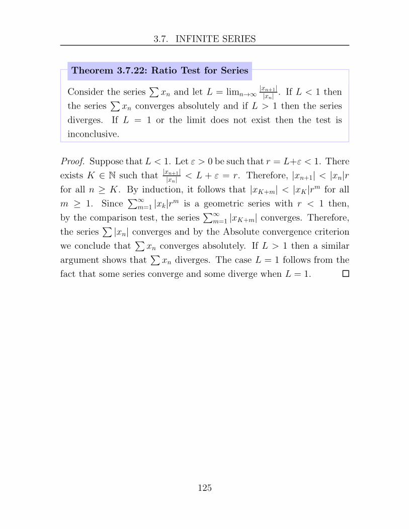
3.7. INFINITE SERIES
Theorem 3.7.22: Ratio Test for Series
Consider the series∑xn and let L = limn→∞
|xn+1||xn| . If L < 1 then
the series∑xn converges absolutely and if L > 1 then the series
diverges. If L = 1 or the limit does not exist then the test is
inconclusive.
Proof. Suppose that L < 1. Let ε > 0 be such that r = L+ε < 1. There
exists K ∈ N such that |xn+1||xn| < L + ε = r. Therefore, |xn+1| < |xn|r
for all n ≥ K. By induction, it follows that |xK+m| < |xK |rm for all
m ≥ 1. Since∑∞
m=1 |xk|rm is a geometric series with r < 1 then,
by the comparison test, the series∑∞
m=1 |xK+m| converges. Therefore,
the series∑ |xn| converges and by the Absolute convergence criterion
we conclude that∑xn converges absolutely. If L > 1 then a similar
argument shows that∑xn diverges. The case L = 1 follows from the
fact that some series converge and some diverge when L = 1.
125

3.7. INFINITE SERIES
Exercises
Exercise 3.7.1. Suppose that∑xn is a convergent series. Is it true
that if∑yn is divergent then
∑(xn + yn) is divergent? If it is true,
prove it, otherwise give an example to show that it is not true.
Exercise 3.7.2. Suppose that xn ≥ 0 for all n ∈ N. Prove that
if∑∞
n=1 xn converges then∑∞
n=1xn
n also converges. Is the converse
true? That is, if∑∞
n=1xn
n converges then does it necessarily follow
that∑∞
n=1 xn converges?
Exercise 3.7.3. Using only the tests derived in this section, determine
whether the given series converge or diverge:
(a)∞∑
n=1
2n2 + 3√n2 + 3n+ 2
(b)∞∑
n=1
cos(nπ)3n
2n
(c)
∞∑
n=1
1
n!
(d)
∞∑
n=1
n− 3
n3 + 1
Exercise 3.7.4. Suppose that (xn) and (yn) are non-negative sequences.
Prove that if∑xn and
∑yn are convergent then
∑xnyn is convergent.
(Hint: Recall that if zn ≥ 0 then∑zn converges iff (sn) is bounded,
where sn =∑n
k=1 zk is the sequence of partial sums. Alternatively, use
the identity (x+ y)2 = x2 + 2xy + y2.)
Exercise 3.7.5. Suppose that xn > 0 for all n ∈ N and∑∞
n=1 xn
converges. You will prove that∑∞
n=1
√xnxn+1 converges.
126
3.7. INFINITE SERIES
(a) Let yn = xn + xn+1. Prove that∑∞
n=1 yn converges.
(b) Using the fact that (a+b)2 = a2+2ab+b2, prove that√ab ≤ a+b
if a, b > 0. Deduce that
√xnxn+1 ≤ xn + xn+1 = yn.
(c) Deduce that∑∞
n=1
√xnxn+1 converges.
Exercise 3.7.6. Any number of the form x = 0.a1a2a3a4 . . . can be
written as
x =a110
+a2102
+a3103
+a4104
+ · · ·
Using this fact, and a geometric series, prove that
0.25555555555555555 . . . . . . . . . =23
90.
Exercise 3.7.7. Show that the following series converge and find their
sum.
(a)
∞∑
n=0
(−1)n
e2n
(b)
∞∑
j=2
3
2j
(c)∞∑
k=−2
1
3k
Exercise 3.7.8. Using the fact that 2k−1 < k! for all k ≥ 3, prove that
the series∑∞
n=01n! converges.
127

3.7. INFINITE SERIES
128

4
Limits
You are familiar with computing limits of functions from calculus. As
you may recall, a function f has limit L at a point c if the outputs f(x)
are arbitrarily close to L provided the inputs x are sufficiently close to
c. Although this notion is intuitive, we will give a precise definition of
the limit of a function and we will relate the definition with limits of
sequences.
4.1 Limits of Functions
Recall that when computing
limx→c
f(x)
the function f need not be defined at x = c. The reason for this is that
many limits of interest arise when f is not defined at x = c, for example
when computing derivatives. However, in order for the limit notion to
make sense, it is necessary that f be defined for points arbitrarily close
to c. This motivates the following definition.
129
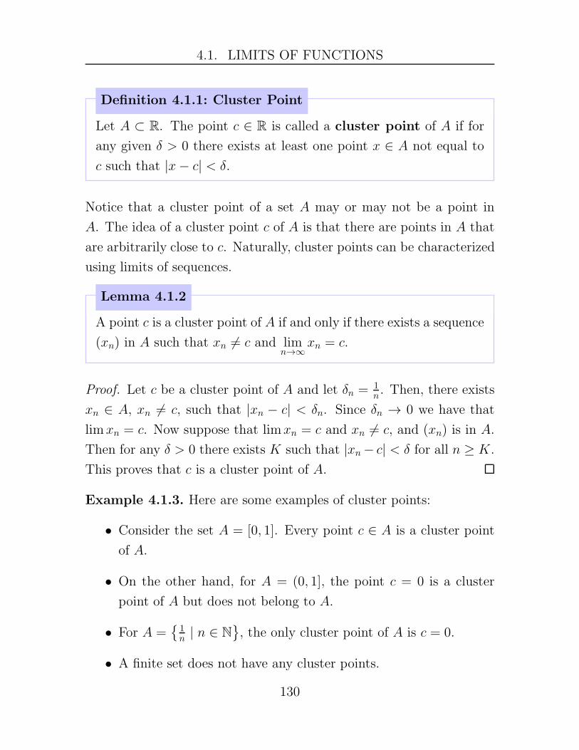
4.1. LIMITS OF FUNCTIONS
Definition 4.1.1: Cluster Point
Let A ⊂ R. The point c ∈ R is called a cluster point of A if for
any given δ > 0 there exists at least one point x ∈ A not equal to
c such that |x− c| < δ.
Notice that a cluster point of a set A may or may not be a point in
A. The idea of a cluster point c of A is that there are points in A that
are arbitrarily close to c. Naturally, cluster points can be characterized
using limits of sequences.
Lemma 4.1.2
A point c is a cluster point of A if and only if there exists a sequence
(xn) in A such that xn 6= c and limn→∞
xn = c.
Proof. Let c be a cluster point of A and let δn = 1n. Then, there exists
xn ∈ A, xn 6= c, such that |xn − c| < δn. Since δn → 0 we have that
limxn = c. Now suppose that limxn = c and xn 6= c, and (xn) is in A.
Then for any δ > 0 there exists K such that |xn− c| < δ for all n ≥ K.
This proves that c is a cluster point of A.
Example 4.1.3. Here are some examples of cluster points:
• Consider the set A = [0, 1]. Every point c ∈ A is a cluster point
of A.
• On the other hand, for A = (0, 1], the point c = 0 is a cluster
point of A but does not belong to A.
• For A ={1n | n ∈ N
}, the only cluster point of A is c = 0.
• A finite set does not have any cluster points.
130

4.1. LIMITS OF FUNCTIONS
• The set A = N has no cluster points.
• Consider the set A = Q ∩ [0, 1]. By the Density theorem, every
point c ∈ [0, 1] is a cluster point of A.
We now give the definition of the limit of a function f : A → R at
a cluster point c of A. In this chapter, the letter A will denote a subset
of R.
Definition 4.1.4: Limit of a Function
Consider a function f : A → R and let c be a cluster point of A.
We say that f has limit at c, or converges at c, if there exists
a number L ∈ R such that for any given ε > 0 there exists δ > 0
such that if x ∈ A and 0 < |x− c| < δ then |f(x)− L| < ε. In this
case, we write that
limx→c
f(x) = L
and we say that f converges to L at c, or that f has limit L at
c. If f does not converge at c then we say that it diverges at c.
Another short-hand notation to say that f converges to L at c is f(x) →L as x→ c.
By definition, if limx→c f(x) = L, then for any ε > 0 neighborhood
of L, there exists a δ > 0 neighborhood of c such that for all x ∈(c− δ, c+ δ) ∩ A not equal to c it is true that f(x) ∈ (L− ε, L+ ε).
Theorem 4.1.5: Uniqueness of Limits
A function f : A→ R can have at most one limit at c.
Proof. Suppose that f(x) → L and f(x) → L′ as x → c. Let ε > 0.
Then there exists δ > 0 such that |f(x)−L| < ε/2 and |f(x)−L′| < ε/2,
131

4.1. LIMITS OF FUNCTIONS
for 0 < |x− c| < δ. Then if 0 < |x− c| < δ then
|L− L′| ≤ |f(x)− L|+ |f(x)− L′|< ε/2 + ε/2
= ε.
Since ε is arbitrary, Theorem 2.2.7 implies that L = L′.
Example 4.1.6. Prove that limx→2
(5x+ 3) = 13.
Proof. We begin by analyzing the quantity |f(x)− L|:
|5x+ 3− 13| = |5x− 10|= 5|x− 2|.
Hence, if 0 < |x− 2| < ε/5 then
|5x+ 3− 13| = 5|x− 2|< 5(ε/5)
= ε
Example 4.1.7. Prove that limx→1
x+ 1
x2 + 3=
1
2.
Proof. We have that∣∣∣∣
x+ 1
x2 + 3− 1
2
∣∣∣∣=
∣∣∣∣
x2 − 2x+ 1
2(x2 + 3)
∣∣∣∣
=|x− 1|22(x2 + 3)
< |x− 1|2.
132

4.1. LIMITS OF FUNCTIONS
Let ε > 0 be arbitrary and let δ =√ε. Then if 0 < |x − 1| < δ then
|x− 1|2 < (√ε)2 = ε. Hence, if 0 < |x− 1| < δ then
∣∣∣∣
x+ 1
x2 + 3− 1
2
∣∣∣∣< |x− 1|2 < ε.
Example 4.1.8. Prove that limx→c
x2 = c2.
Proof. We have that
|x2 − c2| = |x + c||x− c|.
By the triangle inequality, |x + c| ≤ |x|+ |c| and therefore
|x2 − c2| = |x+ c||x− c|≤ (|x|+ |c|)|x− c|.
We now obtain a bound for |x| + |c| when x is say within δ1 > 0 of c.
Hence, suppose that 0 < |x− c| < δ1. Then
|x| = |x− c+ c|≤ |x− c|+ |c|< δ1 + |c|
and therefore |x + c| ≤ |x| + |c| < δ1 + 2|c|. Suppose that ε > 0 is
arbitrary and let δ = min{δ1, ε/(δ1 + 2|c|)}. Then if 0 < |x − c| < δ
then |x+ c| < δ1 + 2|c| and therefore
|x2 − c2| = |x + c||x− c|< (δ1 + 2|c|)δ≤ (δ1 + 2|c|)ε/(δ1 + 2|c|)= ε.
133

4.1. LIMITS OF FUNCTIONS
Example 4.1.9. Prove that limx→6
x2 − 3x
x+ 3= 2.
Proof. We have that∣∣∣∣
x2 − 3x
x+ 3− 2
∣∣∣∣=
∣∣∣∣
x2 − 5x− 6
x+ 3
∣∣∣∣
=
∣∣∣∣
(x+ 1)(x− 6)
(x+ 3)
∣∣∣∣
=|x + 1||x + 3||x− 6|.
We now obtain a bound for |x+1||x+3| when x is close to 6. Suppose then
that |x − 6| < 1. Then 5 < x < 7. Therefore, 6 < x + 1 < 8, and
therefore |x+ 1| < 8. Similarly, if |x− 6| < 1 then 8 < x+ 3 < 10 and
therefore 8 < |x + 3| and therefore 1|x+3| <
18. Therefore, if |x − 6| < 1
then|x+ 1||x+ 3| < 8 · 1
8= 1.
Suppose that ε > 0 is arbitrary and let δ = min{1, ε}. If 0 < |x−6| < δ
then from above we have that |x+1||x+3| < 1, and clearly |x − 6| ≤ ε.
Therefore, if 0 < |x− 6| < δ then∣∣∣∣
x2 − 3x
x+ 3− 2
∣∣∣∣=
|x+ 1||x+ 3||x− 6|
< |x− 6|≤ ε.
This ends the proof.
Example 4.1.10. Prove that limx→−2
x2 − 3x
x+ 3= 10.
The following important result states that limits of functions can
be studied using limits of sequences.
134

4.1. LIMITS OF FUNCTIONS
Theorem 4.1.11: Sequential Criterion for Limits
Let f : A → R be a function and let c be a cluster point of A.
Then limx→c f(x) = L if and only if for every sequence (xn) in A
converging to c the sequence (f(xn)) converges to L (with xn 6= c).
Proof. Suppose that f(x) → L as x → c. Let (xn) be a sequence in
A converging to c, with xn 6= c. Let ε be given. Then there exists
δ > 0 such that if 0 < |x − c| < δ then |f(x) − L| < ε. Now, since
(xn) → c, there exists K ∈ N such that |xn − c| < δ for all n ≥ K.
Therefore, for n ≥ K we have that |f(xn) − L| < ε. This proves that
limn→∞ f(xn) = L.
To prove the converse, we prove the contrapositive. Hence, we show
that if f does not converge to L then there exists a sequence (xn) in
A (with xn 6= c) converging to c but the sequence (f(xn)) does not
converge to L. Assume then that f does not converge to L. Then there
exists ε > 0 such for all δ > 0 there exists x such that 0 < |x − c| < δ
and |f(x) − L| ≥ ε. Let δn = 1n . Then there exists xn 6= c such that
0 < |xn − c| < δn and |f(xn)− L| ≥ ε. Hence (xn) → c but f(xn) does
not converge to L.
The following theorem follows immediately from Theorem 4.1.11.
Corollary 4.1.12
Let f : A → R be a function and let c be a cluster point of A and
let L ∈ R. Then f does not converge to L at c if and only if there
exists a sequence (xn) in A converging c, with xn 6= c, and such that
f(xn) does not converge to L.
Note that in the previous corollary, if the sequence (f(xn)) diverges
then it clearly does not converge to any L ∈ R and then f does not
135

4.1. LIMITS OF FUNCTIONS
have a limit at c. When applicable, the following corollary is a useful
tool to prove that a limit of a function does not exist.
Corollary 4.1.13
Let f : A → R be a function and let c be a cluster point of A.
Suppose that (xn) and (yn) are sequences in A converging to c, with
xn 6= c and yn 6= c. If f(xn) and f(yn) converge but limn→∞
f(xn) 6=limn→∞
f(yn) then f does not have a limit at c.
Example 4.1.14. Prove that limx→01x does not exist.
Proof. Consider xn = 1n, which clearly converges to c = 0 and xn 6= 0.
Then f(xn) = n which does not converge.
Example 4.1.15. Prove that limx→0 sin(1x
)does not exist.
Proof. Let f(x) = sin(1x
). Consider the sequence xn = 1
π/2+nπ. It is
clear that (xn) → 0 and xn 6= 0 for all n. Now (f(xn)) = (−1, 1,−1,−1, . . . , )
and therefore (f(xn)) does not converge. Therefore, f has no limit at
c = 0. In fact, for each α ∈ [0, 2π), consider the sequence xn = 1α+2nπ .
Clearly (xn) → 0 and xn 6= 0 for all n. Now, f(xn) = sin(α + 2nπ) =
sin(α). Hence, (f(xn)) converges to sin(α). This shows that f oscillates
within the interval [−1,−1] as x approaches c = 0.
Example 4.1.16. The sgn(x) function is defined as
sgn(x) =
|x|x, if x 6= 0
0, if x = 0.
Prove that limx→0 sgn(x) does not exist.
Proof. Let xn = (−1)n
n . Then (xn) → 0 and xn 6= 0 for all n. Now,
yn = sgn(xn) = (−1)n. Clearly, (yn) does not converge and thus sgn
has no limit at c = 0.
136

4.1. LIMITS OF FUNCTIONS
Exercises
Exercise 4.1.1. Use the ε-δ definition of the limit of a function to
verify the following limits.
(a) limx→3
2x+ 3
4x− 9= 3
(b) limx→6
x2 − 3x
x+ 3= 2
(c) limx→4
|x− 3| = 1
Exercise 4.1.2. Let A ⊂ R, let f : A → R, and suppose that c is a
cluster point of A. Suppose that there exists a constant K > 0 such
that |f(x)− L| ≤ K|x− c| for all x ∈ A. Prove that limx→c
f(x) = L.
Exercise 4.1.3. Consider the function
f(x) =
x2 sin(1/x), x ∈ Q\{0}x2
1+x2 , x /∈ Q
Prove that limx→0 f(x) = 0.
Exercise 4.1.4. Let f : R → R be defined as follows:
f(x) =
x, if x ∈ Q
−x, if x ∈ R\Q
(a) Prove that f has a limit at c = 0.
(b) Now suppose that c 6= 0. Prove that f has no limit at c.
(c) Define g : R → R by g(x) = (f(x))2. Prove that g has a limit at
any c ∈ R.
137
4.1. LIMITS OF FUNCTIONS
Hint: The Density Theorem will be helpful for (b). In particular, the
Density Theorem implies that for any point c ∈ R, there exists a se-
quence (xn) of rational numbers such that (xn) → c, and that there
exists a sequence (yn) of irrational numbers such that (yn) → c.
Exercise 4.1.5. Use any applicable theorem to explain why the fol-
lowing limits do not exist.
(a) limx→01x2
(b) limx→0(x+ sgn(x))
(c) limx→0 sin(1/x2)
The sgn function is defined as follows:
sgn(x) =
{
1, x ≥ 0
−1, x < 0
138

4.2. LIMIT THEOREMS
4.2 Limit Theorems
We first show that if f has a limit at c then it is locally bounded at c.
We first define what it means to be locally bounded.
Definition 4.2.1: Local Boundedness
Let f : A → R and let c be a cluster point of A. We say that f is
bounded locally at c if there exists δ > 0 and M > 0 such that
if x ∈ (c− δ, c+ δ) ∩ A then |f(x)| ≤M .
Theorem 4.2.2
Let f : A → R be a function and let c be a cluster point of A. If
limx→c
f(x) exists then f is bounded locally at c.
Proof. Let L = limx→c f(x) and let ε > 0 be arbitrary. Then there
exists δ > 0 such that |f(x) − L| < ε for all x ∈ A such that 0 <
|x− c| < δ. Therefore, for all x ∈ A and 0 < |x− c| < δ we have that
|f(x)| = |f(x)− L+ L|≤ |f(x)− L|+ |L|< ε+ |L|.
If c ∈ A then let M = max{|f(c)|, ε + |L|} and if c /∈ A then let
M = ε+ |L|. Then |f(x)| ≤M for all x ∈ A such that 0 < |x− c| < δ,
that is, f is bounded locally at c.
Example 4.2.3. Consider again the function f(x) = 1x defined on the
set A = (0,∞). Clearly, c = 0 is a cluster point of A. For any δ > 0
and any M > 0 let x ∈ A be such that 0 < x < min{δ, 1M }. Then
139

4.2. LIMIT THEOREMS
0 < x < 1M , that is, M < 1
x = f(x). Since M was arbitrary, this proves
that f is unbounded at c = 0 and consequently f does not have a limit
at c = 0.
We now consider Limit Laws for functions. Let f, g : A → R be
functions and define
(f ± g)(x) = f(x)± g(x)
(fg)(x) = f(x)g(x)
(f
g
)
(x) =f(x)
g(x)
where for the ratio f/g we require that g(x) 6= 0 for all x ∈ A.
Theorem 4.2.4: Limit Laws
Let f, g : A → R be functions and let c be a cluster point of A.
Suppose that limx→c f(x) = L and limx→c g(x) =M . Then
(i) limx→c
(f ± g)(x) = L±M
(ii) limx→c
(fg)(x) = LM
(iii) limx→c
(f
g
)
(x) =L
M, if M 6= 0
The proofs are left as an exercises. (To prove the results, use the
sequential criterion for limits and the limits laws for sequences).
140
4.2. LIMIT THEOREMS
Corollary 4.2.5
Let f1, . . . , fk : A → R be functions and let c be a cluster point of
A. If limx→c fi(x) exists for each i = 1, 2, . . . , k then
(i) limx→c
k∑
i=1
fi(x) =k∑
i=1
limx→c
fi(x)
(ii) limx→c
k∏
i=1
fi(x) =k∏
i=1
limx→c
fi(x)
Example 4.2.6. If f(x) = a0+ a1x+ a2x2+ · · ·+ anx
n is a polynomial
function then limx→c f(x) = f(c) for every c ∈ R. If g(x) = b0 + b1x +
b2x + · · · + bmxm is another polynomial function and g(x) 6= 0 in a
neighborhood of x = c and limx→c g(x) = g(c) 6= 0 then
limx→c
f(x)
g(x)=f(c)
g(c).
Example 4.2.7. Prove that limx→2
x2 − 4
x− 2= 4.
Proof. We cannot use the Limit Laws directly since limx→2(x− 2) = 0.
Now, if x 6= 2 then x2−4x−2 = x + 2. Hence, the functions f(x) = x2−4
x−2
and g(x) = x + 2 agree at every point in R\{0}. It is clear that
limx→2 g(x) = 4. Let ε > 0 and let δ > 0 be such that if 0 < |x− 2| < δ
then |g(x)− 4| < ε. Then for 0 < |x− 2| < δ we have that |f(x)− 4| =|g(x)− 4| < ε. Hence limx→2 f(x) = 4.
Theorem 4.2.8
Let f : A → R be a function and let c be a cluster point of A.
Suppose that f has limit L at c. If f(x) ≥ 0 for all x ∈ A then
L ≥ 0.
141

4.2. LIMIT THEOREMS
Proof. We prove the contrapositive. Suppose that L < 0. Let ε > 0 be
such that L+ε < 0. There exists δ > 0 such that if 0 < |x−c| < δ then
f(x) < L + ε < 0. Hence, f(x) < 0 for some x ∈ A. An alternative
proof: If f converges to L at c then for any sequence (xn) converging
to c, xn 6= 0, we have that f(xn) → L. Now f(xn) ≥ 0 and therefore
L ≥ 0 from our results on limits of sequences.
Theorem 4.2.9
Let f : A → R be a function and let c be a cluster point of A.
Suppose that M1 ≤ f(x) ≤ M2 for all x ∈ A and suppose that
limx→c f(x) = L. Then M1 ≤ L ≤M2.
Proof. We have that 0 ≤ f(x) −M1 and therefore by Theorem 4.2.8
we have that 0 ≤ L −M1. Similarly, from 0 ≤ M2 − f(x) we deduce
that 0 ≤ M2 − L. From this we conclude that M1 ≤ L ≤ M2. An
alternative proof: Since f → L at c, for any sequence (xn) → c with
xn 6= 0, we have that f(xn) → L. Clearly, M1 ≤ f(xn) ≤ M2 and
therefore M1 ≤ L ≤M2.
The following is the Squeeze Theorem for functions.
Theorem 4.2.10: Squeeze Theorem
Let f, g, h : A → R be functions and let c be a cluster point of A.
Suppose that limx→c
g(x) = L and limx→c
h(x) = L. If g(x) ≤ f(x) ≤ h(x)
for all x ∈ A, x 6= c, then limx→c
f(x) = L.
Proof. Let (xn) be a sequence in A converging to c, xn 6= c. Then L =
lim g(xn) = limh(xn). Clearly g(xn) ≤ f(xn) ≤ h(xn), and therefore by
the Squeeze Theorem for sequences we have that lim f(xn) = L. This
holds for every such sequence and therefore f → L at c.
142
4.2. LIMIT THEOREMS
Example 4.2.11. Let
f(x) =
x2 sin(1/x), x ∈ Q\{0}
x2 cos(1/x), x /∈ Q
0, x = 0.
Show that limx→0 f(x) = 0.
We end this section with the following theorem.
Theorem 4.2.12
Let f : A → R be a function and let c be a cluster point of A.
Suppose that limx→c f(x) = L. If L > 0 then there exists δ > 0
such that f(x) > 0 for all x ∈ (c− δ, c+ δ), x 6= c.
Proof. Choose ε > 0 so that L−ε > 0, take for example ε = L/2. Then
there exists δ > 0 such that L−ε < f(x) < L+ε for all x ∈ (c−δ, c+δ),x 6= c.
143

4.2. LIMIT THEOREMS
Exercises
Exercise 4.2.1. Let f, g : A → R and suppose that c ∈ R is a cluster
point of A. Suppose that at c, f converges to L and g converges to
M . Prove that fg converges to LM at c in two ways: (1) using the ε-δ
definition, and (2) using the sequential criterion for limits.
Exercise 4.2.2. Give an example of a set A ⊂ R, a cluster point c of
A, and two functions f, g : A → R such that limx→c
f(x)g(x) exists but
limx→c
f(x) does not exist.
Exercise 4.2.3. Give an example of a function f : R → R that is
bounded locally at c = 0 but does not have a limit at c = 0. Your
answer should not be in the form of a graph.
Exercise 4.2.4. Let f : R → R be a function that is bounded locally
at c and suppose that g : R → R converges to L = 0 at c. Prove that
limx→c
f(x)g(x) = 0.
144
5
Continuity
Throughout this chapter, A is a non-empty subset of R and f : A→ R
is a function.
5.1 Continuous Functions
Definition 5.1.1: Continuity
The function f is continuous at c ∈ A if for any given ε > 0 there
exists δ > 0 such that if x ∈ A and |x−c| < δ then |f(x)−f(c)| < ε.
If f is not continuous at c then we say that f is discontinuous at
c. The function f is continuous on A if f is continuous at every
point in A.
Suppose that c ∈ A is a cluster point of A and f is continuous at
c. Then from the definition of continuity, limx→c
f(x) exists and equal to
f(c). If c is not a cluster point of A then there exists δ > 0 such that
(c− δ, c+ δ)∩A = {c} and continuity of f at c is immediate. In either
case, we see that f is continuous at c if and only if
limx→c
f(x) = f(c)
145

5.1. CONTINUOUS FUNCTIONS
The following is then immediate.
Theorem 5.1.2: Sequential Criterion for Continuity
The function f is continuous at c ∈ A if and only if for every
sequence (xn) in A converging to c, f(xn) converges to f(c):
limn→∞
f(xn) = f( limx→∞
xn) = f(c).
Notice that here (xn) is allowed to take on the value c. The following
is immediate.
Theorem 5.1.3
The function f is discontinuous at c if and only if there exists a
sequence (xn) in A converging to c but f(xn) does not converge to
f(c).
Example 5.1.4. If f(x) = a0+ a1x+ a2x2+ · · ·+ anx
n is a polynomial
function then limx→c f(x) = f(c) for every c ∈ R. Thus, f is continuous
everywhere. If g(x) = b0+ b1x+ b2x+ · · ·+ bmxm is another polynomial
function and g(c) 6= 0 then
limx→c
f(x)
g(x)=f(c)
g(c).
Hence, h(x) = f(x)/g(x) is continuous at every c where g is non-zero.
Example 5.1.5. Determine the points of continuity of
f(x) =
1x, x 6= 0
0, x = 0.
146

5.1. CONTINUOUS FUNCTIONS
Solution. Suppose that c 6= 0. Then limx→c f(x) =1c = f(c). Hence,
f is continuous at c ∈ R\{0}. Consider now c = 0. The sequence
xn = 1nconverges to c = 0 but f(xn) = n does not converge. Hence,
limx→0 f(x) does not exist. Thus, even though f(0) = 0 is well-defined,
f is discontinuous at c = 0.
Example 5.1.6 (Dirichlet Function). The following function was con-
sidered by Peter Dirichlet in 1829:
f(x) =
1, x ∈ Q
0, x ∈ R\Q(5.1)
Prove that f is discontinuous everywhere.
Proof. Let c be irrational and let ε = 1/2. Then for all δ > 0, there
exists x ∈ Q ∩ (c − δ, c + δ) (by the Density theorem) and therefore
|f(x) − f(c)| = 1 > ε. Hence, f is discontinuous at c. A similar
argument shows that f is discontinuous c ∈ Q. Alternatively, if c ∈ Q
then there exists a sequence of irrational numbers (xn) converging to c.
Now f(xn) = 0 and f(c) = 1, and this proves that f is discontinuous
at c. A similar arguments holds for c irrational.
Example 5.1.7 (Thomae Function). Let A = {x ∈ R : x > 0} and
define f : A→ R as
f(x) =
0, x ∈ R\Q,1n , x = m
n ∈ Q, gcd(m, n) = 1, n ∈ N
The graph of f is shown in Figure 5.1. Prove that f is continuous
at every irrational number in A and is discontinuous at every rational
number in A.
147

5.1. CONTINUOUS FUNCTIONS
-1 -0.75 -0.50 -0.25 0.25 0.50 0.75 1
0.2
0.3
0.4
0.5
Figure 5.1: Thomae’s function is continuous at each irrational anddiscontinuous at each rational
Proof. Let c = mn ∈ Q with gcd(m, n) = 1. There exists a sequence
(xn) of irrational numbers in A converging to c. Hence, f(xn) = 0
while f(c) = 1n. This shows that f is discontinuous at c. Now let c be
irrational and let ε > 0 be arbitrary. Let N ∈ N be such that 1N < ε.
In the interval (c− 1, c+1), there are only a finite number of rationalsmn with n < N , otherwise we can create a sequence mk
nkwith nk < N , all
the rationals mk
nkdistinct and thus necessarily mk
nkis unbounded. Hence,
there exists δ > 0 such that the interval (c − δ, c + δ) contains only
rational numbers x = mn with n > N . Hence, if x = m
n ∈ (c− δ, c + δ)
then f(x) = 1n < 1
N and therefore |f(x) − f(c)| = 1n < 1
N < ε. On
the other hand, if x ∈ (c − δ, c + δ) is irrational then |f(x) − f(c)| =|0− 0| < ε. This proves that f is continuous at c.
Suppose that f has a limit L at c but f is not defined at c. We can
148

5.1. CONTINUOUS FUNCTIONS
extend the definition of f by defining
F (x) =
f(x), x 6= c
L, x = c.
Now, limx→c F (x) = limx→c f(x) = L = F (c), and thus F is continuous
at c. Hence, functions that are not defined at a particular point c but
have a limit at c can be extended to a function that is continuous at c.
Points of discontinuity of this type are called removal singularities.
On the other hand, the function f(x) = sin(1/x) is not defined at c = 0
and has not limit at c = 0, and therefore cannot be extended at c = 0
to a continuous function.
149
5.1. CONTINUOUS FUNCTIONS
Exercises
Exercise 5.1.1. Let
f(x) =
{
x2 sin(1/x), x 6= 0
0, x = 0
Prove that f is continuous at c = 0.
Exercise 5.1.2. Let
f(x) =
{
(1/x) sin(1/x2), x 6= 0
0, x = 0
Prove that f is discontinuous at c = 0.
Exercise 5.1.3. This is an interesting exercise.
(a) Suppose that h : R → R is continuous on R and that h(r) = 0
for every rational number r ∈ Q. Prove that in fact h(x) = 0 for
all x ∈ R.
(b) Let f, g : R → R be continuous functions on R such that f(r) =
g(r) for every rational number r ∈ Q. Prove that in fact f(x) =
g(x) for all x ∈ R. Hint: Part (a) will be useful here.
Exercise 5.1.4. Suppose that f : R → R is a continuous function such
that f(p + q) = f(p) + f(q) for every p, q ∈ Q. Prove that in fact
f(x+ y) = f(x) + f(y) for every x, y ∈ R.
150
5.2. COMBINATIONS OF CONTINUOUS FUNCTIONS
5.2 Combinations of Continuous Functions
Not surprisingly, the set of continuous functions is closed under the
basic operation of arithmetic.
Theorem 5.2.1
Let f, g : A → R be continuous functions at c ∈ A and let b ∈ R.
Then
(i) f + g, f − g, fg, and bf are continuous at c.
(ii) If h : A→ R is continuous at c ∈ A and h(x) 6= 0 for all x ∈ A
then fh is continuous at c.
Proof. Let ε > 0 be arbitrary. By continuity of f and g at c, there
exists δ1 > 0 such that |f(x) − f(c)| < ε/2 for all x ∈ A such that
0 < |x− c| < δ1, and there exists δ2 > 0 such that |g(x)− g(c)| < ε/2
for all x ∈ A such that 0 < |x− c| < δ2. Let δ = min{δ1, δ2}. Then for
x ∈ A such that 0 < |x− c| < δ we have that
|f(x) + g(x)− (f(c) + g(c))| ≤ |f(x)− f(c)|+ |g(x)− g(c)|< ε/2 + ε/2
= ε.
This proves that f + g is continuous at c. A similar proof holds for
f − g.
Consider now the function bf . If b = 0 then bf(x) = 0 for all x ∈ A
and continuity is trivial. So assume that b 6= 0. Let ε > 0 be arbitrary.
Then there exists δ > 0 such that if x ∈ A ∩ (c− δ, c+ δ), x 6= c, then
|f(x)− f(c)| < ε/(|b|). Therefore, for x ∈ A ∩ (c− δ, c+ δ), x 6= c, we
151

5.2. COMBINATIONS OF CONTINUOUS FUNCTIONS
have that
|bf(x)− bf(c)| = |b||f(x)− f(c)|< |b|ε/(|b|)= ε.
We now prove continuity of fg. Let (xn) be any sequence in A
converging to c. Then yn = f(xn) converges to f(c) by continuity of f
at c, and zn = g(xn) converges to g(c) by continuity of g at c. Hence the
sequence wn = ynzn converges to f(c)g(c). Hence, for every sequence
(xn) converging to c, f(xn)g(xn) converges to f(c)g(c). This shows that
fg is continuous at c.
Corollary 5.2.2
Let f, g : A→ R be continuous functions on A and let b ∈ R. Then
(i) f + g, f − g, fg, and bf are continuous on A.
(ii) If h : A → R is continuous on A and h(x) 6= 0 for all x ∈ A
then fh is continuous on A.
Example 5.2.3. Prove that f(x) = x is continuous on R.
Proof. Let ε > 0 be arbitrary. Let δ = ε. If 0 < |x − c| < δ then
|f(x)− f(c)| = |x− c| < δ = ε.
Example 5.2.4. All polynomials p(x) = a0 + a1x + · · · + anxn are
continuous everywhere.
Example 5.2.5. Rational functions f(x) = p(x)/q(x), with q(x) 6= 0
on A ⊂ R, are continuous on A.
152

5.2. COMBINATIONS OF CONTINUOUS FUNCTIONS
Lemma 5.2.6: Continuity Under Shifting
If f : R → R is continuous then g(x) = f(x + α) is continuous,
where α ∈ R is arbitrary.
Proof. Let ε > 0 be arbitrary. Then there exists δ > 0 such that
|f(y) − f(d)| < ε for all 0 < |y − d| < δ. Therefore, if 0 < |x − c| =|(x+ α)− (c+ α)| < δ then |f(x+ α)− f(c+ α)| < ε and therefore
|g(x)− g(c)| = |f(x+ α)− f(c+ α)| < ε.
To prove continuity of sin(x) and cos(x) we use the following facts.
For all x ∈ R, | sin(x)| ≤ |x| and | cos(x)| ≤ 1, and for all x, y,∈ R
sin(x)− sin(y) = 2 sin(12(x− y)
)cos(12(x+ y)
).
Example 5.2.7. Prove that sin(x) and cos(x) are continuous every-
where.
Proof. We have that
| sin(x)− sin(c)| ≤ 2| sin(12(x− c))|| cos(1
2(x− c))|
≤ 21
2|x− c|
= |x− c|.
Hence given ε > 0 we choose δ = ε. The proof that cos(x) is continuous
follows from the fact that cos(x) = sin(x+ π/2) and Lemma 5.2.6.
Example 5.2.8. The functions tan(x) = sin(x)cos(x)
, cot(x) = cos(x)sin(x)
, sec(x) =1
cos(x) , and csc(x) = 1sin(x) are continuous on their domain.
153

5.2. COMBINATIONS OF CONTINUOUS FUNCTIONS
Example 5.2.9. Prove that f(x) =√x is continuous on A = {x ∈
R | x ≥ 0}.
Proof. For c = 0, we must consider |√x−√0| = √
x. Given ε > 0 let
δ = ε2. Then if x ∈ A and x < δ = ε2 then√x < ε. This shows that f
is continuous at c = 0. Now suppose that c 6= 0. Then
|√x−√c| = |√x−√
c| ·√x+
√c√
x+√c
=|x− c|√x+
√c
≤ 1√c|x− c|.
Hence, given ε > 0, suppose that 0 < |x− c| < √cε. Then |√x−√
c| <ε.
Example 5.2.10. Prove that f(x) = |x| is continuous everywhere.
Proof. Follows from the inequality ||x| − |c|| ≤ |x− c|.
The last theorem of this section is concerned with the composition
of continuous functions.
Theorem 5.2.11: Continuity of Composite Functions
Let f : A → R and let g : B → R be continuous functions and
suppose that f(A) ⊂ B. Then the composite function (g ◦f) : A→R is continuous.
Proof. Let ε > 0 be given. Let c ∈ A and let d = f(c) ∈ B. Then there
exists δ1 > 0 such that if 0 < |y − d| < δ1 then |g(y) − g(d)| < ε. Now
since f is continuous at c, there exists δ2 > 0 such that if 0 < |x−c| < δ2
154

5.3. CONTINUITY ON CLOSED INTERVALS
then |f(x)−f(c)| < δ1. Therefore, if 0 < |x−c| < δ2 then |f(x)−d| < δ1
and therefore |g(f(x))−g(d)| < ε. This proves that (g◦f) is continuousat c ∈ A. Since c is arbitrary, (g ◦ f) is continuous on A.
Corollary 5.2.12
If f : A → R is continuous then g(x) = |f(x)| is continuous. If
f(x) ≥ 0 for all x ∈ A then h(x) =√
f(x) is continuous.
5.3 Continuity on Closed Intervals
In this section we develop properties of continuous functions on closed
intervals.
Definition 5.3.1
We say that f : A → R is bounded on A if there exists M > 0
such that |f(x)| ≤ M for all x ∈ A.
If f is not bounded on A then for any given M > 0 there exists x ∈ A
such that |f(x)| > M .
Example 5.3.2. Consider the function f(x) = 1xdefined on the interval
A = (0,∞). Let M > 0 be arbitrary. Then if 0 < x < 1M then
f(x) = 1x > M . For instance, take x = 1
M+1. However, on the interval
[2, 3], f is bounded by M = 12.
Theorem 5.3.3
Let f : A → R be a continuous function. If A = [a, b] is a closed
and bounded interval then f is bounded on A.
155

5.3. CONTINUITY ON CLOSED INTERVALS
Proof. Suppose that f is unbounded. Then for each n ∈ N there exists
xn ∈ [a, b] such that |f(xn)| > n. Now the sequence (xn) is bounded
since a ≤ xn ≤ b. By the Bolzano-Weierstrass theorem, (xn) has a
convergent subsequence, say (xnk), whose limit u = limk→∞ xnk
satisfies
a ≤ u ≤ b. Since f is continuous at u then limk→∞ f(xnk) exists and
equal to f(u). This is a contradiction since |f(xnk)| > nk ≥ k implies
that f(xnk) is unbounded.
Definition 5.3.4: Extrema of Functions
Let f : A→ R be a function.
(i) The function f has an absolute maximum on A if there
exists x∗ ∈ A such that f(x) ≤ f(x∗) for all x ∈ A. We call
x∗ a maximum point and f(x∗) the maximum value of f
on A.
(ii) The function f has an absolute minimum on A if there
exists x∗ ∈ A such that f(x∗) ≤ f(x) for all x ∈ A. We call
x∗ a minimum point and f(x∗) the minimum value of f
on A.
Suppose that f : [a, b] → R is continuous. By Theorem 5.3.3, the
range of f , that is S = {f(x) | x ∈ [a, b]}, is bounded and therefore
inf(S) and sup(S) exist. In this case, we want to answer the question
as to whether inf(S) and sup(S) are elements of S. In other words, as
to whether f achieves its maximum and/or minimum value on [a, b].
That is, if there exists x∗, x∗ ∈ [a, b] such that f(x∗) ≤ f(x) ≤ f(x∗)
for all x ∈ [a, b].
Example 5.3.5. The function f(x) = 1x is continuous on A = (0, 1].
156

5.3. CONTINUITY ON CLOSED INTERVALS
However, f is unbounded on A and never achieves a maximum value
on A.
Example 5.3.6. The function f(x) = x2 is continuous on [0, 2), is
bounded on [0, 2) but never reaches its maximum value on [0, 2), that
is, if S = {x2 : x ∈ [0, 2)} then sup(S) = 4 /∈ S.
Theorem 5.3.7: Extreme Value Theorem
Let f : A → R be a continuous function. If A = [a, b] is a closed
and bounded interval then f has a maximum and minimum point
on [a, b].
Proof. Let S = {f(x) | x ∈ [a, b]} be the range of f . By Theorem 5.3.3,
sup(S) exists; set M = sup(S). By the definition of the supremum,
for each ε > 0 there exists x ∈ [a, b] such that M − ε < f(x) ≤M . In particular, for εn = 1/n, there exists xn ∈ [a, b] such that
M − εn < f(xn) ≤ M . Then limn→∞ f(xn) = M . The sequence (xn)
is bounded and thus has a convergent subsequence, say (xnk). Let
x∗ = limk→∞ xnk. Clearly, a ≤ x∗ ≤ b. Since f is continuous at x∗, we
have thatM = limk→∞ f(xnk) = f(x∗). Hence, x∗ is a maximum point.
A similar proof establishes that f has a minimum point on [a, b].
By Theorem 5.3.7, we can replace sup{f(x) | x ∈ [a, b]} with
max{f(x) | x ∈ [a, b]}, and inf{f(x) | x ∈ [a, b]} with min{f(x) | x ∈[a, b]}. When the interval [a, b] is clear from the context, we will simply
write max(f) and min(f). The following example shows the importance
of continuity in achieving a maximum/minimum.
Example 5.3.8. The function f : [−1, 1] → R defined by
f(x) =
3− x2, 0 < x ≤ 1
x2, −1 ≤ x ≤ 0
157

5.3. CONTINUITY ON CLOSED INTERVALS
does not achieve a maximum value on the closed interval [−1, 1].
The next theorem, called the Intermediate Value Theorem, is the
main result of this section, and one of the most important results in
this course.
Theorem 5.3.9: Intermediate Value Theorem
Consider the function f : [a, b] → R and suppose that f(a) < f(b).
If f is continuous then for any ξ ∈ R such that f(a) < ξ < f(b)
there exists c ∈ (a, b) such that f(c) = ξ.
Proof. Let S = {x ∈ [a, b] : f(x) < ξ}. The set S is non-empty
because a ∈ S. Moreover, S is clearly bounded above. Let c = sup(S).
By the definition of the supremum, there exists a sequence (xn) in S
such that limn→∞ xn = c. Since a ≤ xn ≤ b it follows that a ≤ c ≤ b.
By definition of xn, f(xn) < ξ and since f is continuous at c we have
that f(c) = limn→∞ f(xn) ≤ ξ, and thus f(c) ≤ ξ. Now let δn > 0 be
such that δn → 0 and c+ δn < b. Then zn = c+ δn converges to c and
ξ ≤ f(zn) because zn 6∈ S. Therefore, since limn→∞ f(zn) = f(c) we
have that ξ ≤ f(c). Therefore, f(c) ≤ ξ ≤ f(c) and this proves that
ξ = f(c). This shows also that a < c < b.
The Intermediate Value Theorem has applications in finding points
where a function is zero.
Corollary 5.3.10
Let f : [a, b] → R be a function and suppose that f(a)f(b) < 0. If
f is continuous then there exists c ∈ (a, b) such that f(c) = 0.
Example 5.3.11. A hiker begins his climb at 7:00 am on a marked
trail and arrives at the summit at 7:00 pm. The next day, the hiker
158

5.3. CONTINUITY ON CLOSED INTERVALS
begins his trek down the mountain at 7:00 am, takes the same trail
down as he did going up, and arrives at the base at 7:00 pm. Use the
Intermediate Value Theorem to show that there is a point on the path
that the hiker crossed at exactly the same time of day on both days.
Proof. Let f(t) be the distance traveled along the trail on the way up
the mountain after t units of time, and let g(t) be the distance remaining
to travel along the trail on the way down the mountain after t units of
time. Both f and g are defined on the same time interval, say [0, 12] if
t is measured in hours. If M is the length of the trail, then f(0) = 0,
f(12) = M , g(0) = M and g(12) = 0. Let h(t) = g(t) − f(t). Then
h(0) = M and h(12) = −M . Hence, there exists t∗ ∈ (0, 12) such that
h(t∗) = 0. In other words, f(t∗) = g(t∗), and therefore t∗ is the time of
day when the hiker is at exactly the same point on the trail.
Example 5.3.12. Prove by the Intermediate Value Theorem that f(x) =
xex − 2 has a root in the interval [0, 1].
Proof. The function f is continuous on [0, 1]. We have that f(0) =
−2 < 0 and f(1) = e− 2 > 0. Therefore, there exists x∗ ∈ (0, 1) such
that f(x∗) = 0, i.e., f has a zero in the interval (0, 1).
The next results says, roughly, that continuous functions preserve
closed and bounded intervals. In the following theorem, we use the
short-hand notation f([a, b]) = {f(x) |x ∈ [a, b]} for the range of f
under [a, b].
Theorem 5.3.13
If f : [a, b] → R is continuous then f([a, b]) = [min(f),max(f)].
Proof. Since f achieves its maximum and minimum value on [a, b], there
exists x∗, x∗ ∈ [a, b] such that f(x∗) ≤ f(x) ≤ f(x∗) for all x ∈ [a, b].
159
5.3. CONTINUITY ON CLOSED INTERVALS
Hence, f([a, b]) ⊂ [f(x∗), f(x∗)]. Assume for simplicity that x∗ < x∗.
Then [x∗, x∗] ⊂ [a, b]. Let ξ ∈ R be such that f(x∗) < ξ < f(x∗). Then
by the Intermediate Value Theorem, there exists c ∈ (x∗, x∗) such that
ξ = f(c). Hence, ξ ∈ f([a, b]), and this shows that [f(x∗), f(x∗)] ⊂f([a, b]). Therefore, f([a, b]) = [f(x∗), f(x∗)] = [min(f),max(f)].
It is worth noting that the previous theorem does not say that
f([a, b]) = [f(a), f(b)].
160

5.3. CONTINUITY ON CLOSED INTERVALS
Exercises
Exercise 5.3.1. Let f : A → R be any function. Show that if −fachieves its maximum at x0 ∈ A then f achieves its minimum at x0.
Exercise 5.3.2. Let f and g be continuous functions on [a, b]. Suppose
that f(a) ≥ g(a) and f(b) ≤ g(b). Prove that f(x0) = g(x0) for at least
one x0 in [a, b].
Exercise 5.3.3. Let f : [0, 1] → R be a continuous function and sup-
pose that f(x) ∈ [0, 1] for all x ∈ [0, 1]. Show that there exists x0 ∈ [0, 1]
such that f(x0) = x0. Hint: Consider the function g(x) = f(x)− x on
the interval [0, 1].
Exercise 5.3.4. Let f : [a, b] → R be a continuous function. Prove that
if f(x) ∈ Q for all x ∈ [a, b] then f is a constant function. Hint: You
will need the Density Theorem and the Intermediate Value Theorem.
161

5.4. UNIFORM CONTINUITY
5.4 Uniform Continuity
In the definition of continuity of f : A → R at c ∈ A, the δ will in
general not only depend on ε but also on c. In other words, given two
points c1, c2 and fixed ε > 0, the minimum δ1 and δ2 needed for c1
and c2 in the definition of continuity are generally going to be different.
To see this, consider the continuous function f(x) = x2. Then it is
straightforward to verify that if c2−ε > 0 then |x2− c2| < ε if and only
if√
c2 − ε− c < x− c <√
c2 + ε− c.
Let c1 = 1 and c2 = 3, and let ε = 1/2. Then |x − 1| < δ1 implies
that |f(x) − f(1)| < ε if and only δ1 ≤√1 + ε − 1 ≈ 0.2247. On the
other hand, |x − c| < δ2 implies that |f(x) − f(3)| < ε if and only if
δ2 ≤√9 + ε − 9 ≈ 0.0822. The reason that a smaller delta is needed
at c = 3 is that the slope of f at c = 3 is larger than that at c = 1.
On the other hand, consider the function f(x) = sin(2x). For any c it
holds that
|f(x)− f(c)| = | sin(2x)− sin(2c)|≤ 2|x− c|.
Hence, given any ε > 0 we can set δ = ε/2 and then |x− c| < δ implies
that |f(x)− f(c)| < ε. The punchline is that δ = ε/2 will work for any
c. These motivating examples lead to the following definition.
Definition 5.4.1: Uniform Continuity
The function f : A → R is said to be uniformly continuous on
A if for each ε > 0 there exists δ > 0 such that for all x, u ∈ A
satisfying |x− u| < δ it holds that |f(x)− f(u)| < ε.
162

5.4. UNIFORM CONTINUITY
Example 5.4.2. Let k 6= 0 be any non-zero constant. Show that
f(x) = kx is uniformly continuous on R.
Proof. We have that |f(x)−f(c)| = |kx−kc| = |k||x−c|. Hence, for anyε > 0 we let δ = ε/|k|, and thus if |x−c| < δ then |f(x)−f(c)| < ε.
Example 5.4.3. Prove that f(x) = sin(x) is uniformly continuous.
Proof. We have that
| sin(x)− sin(c)| ≤ 2| sin(12(x− c))|
≤ |x− c|.
Hence, for ε > 0 let δ = ε and if |x−c| < δ then | sin(x)−sin(c)| < ε.
Example 5.4.4. Show that f(x) =1
1 + x2is uniformly continuous on
R.
Proof. We have that
|f(x)− f(c)| =∣∣∣∣
1
1 + x2− 1
1 + c2
∣∣∣∣
=
∣∣∣∣
1 + c2 − 1− x2
(1 + x2)(1 + c2)
∣∣∣∣
=
∣∣∣∣
x+ c
(1 + x2)(1 + c2)
∣∣∣∣|x− c|
=
∣∣∣∣
x
(1 + x2)(1 + c2)+
c
(1 + x2)(1 + c2)
∣∣∣∣|x− c|.
Now, |x| ≤ 1 + x2 implies that |x|1+x2 ≤ 1 and therefore
|x|(1 + x2)(1 + c2)
≤ 1
1 + c2≤ 1.
163

5.4. UNIFORM CONTINUITY
It follows that |f(x) − f(c)| ≤ 2|x − c|. Hence, given ε > 0 we let
δ = ε/2, and if |x− c| < δ then |f(x)− f(c)| < ε.
The following is a simple consequence of the definition of uniform
continuity.
Theorem 5.4.5
Let f : A→ R be a function. The following are equivalent:
(i) The function f is not uniformly continuous on A.
(ii) There exists ε0 > 0 such that for every δ > 0 there exists
x, u ∈ A such that |x− u| < δ but |f(x)− f(c)| ≥ ε0.
(iii) There exists ε0 > 0 and two sequences (xn) and (un) such that
limn→∞
(xn − un) = 0 and |f(xn)− f(un)| ≥ ε0.
Example 5.4.6. Let f(x) = 1x and let A = (0,∞). Let xn = 1
n and let
un = 1n+1. Then lim(xn − un) = 0. Now |f(xn) − f(un)| = | − 1| = 1.
Hence, if ε = 1/2 then |f(xn) − f(un)| > ε. This proves that f is not
uniformly continuous on A = (0,∞).
Theorem 5.4.7: Uniform Continuity on Intervals
Let f : A → R be a continuous function with domain A = [a, b]. If
f is continuous on A then f is uniformly continuous on A.
Proof. We prove the contrapositive, that is, we will prove that if f is
not uniformly continuous on [a, b] then f is not continuous on [a, b].
Suppose then that f is not uniformly continuous on [a, b]. Then there
exists ε > 0 such that for δn = 1/n, there exists xn, un ∈ [a, b] such
164

5.4. UNIFORM CONTINUITY
that |xn − un| < δn but |f(xn)− f(un)| ≥ ε. Clearly, lim(xn − un) = 0.
Now, since a ≤ xn ≤ b, by the Bolzano-Weierstrass theorem there is a
subsequence (xnk) of (xn) that converges to a point z ∈ [a, b]. Now,
|unk− z| ≤ |unk
− xnk|+ |xnk
− z|
and therefore also limk→∞ unk= z. Hence, both (xnk
) and (unk) are
sequences in [a, b] converging to z but |f(xnk) − f(unk
)| ≥ ε. Hence
f(xnk) and f(unk
) do not converge to the same limit and thus f is not
continuous at z. This completes the proof.
The following example shows that boundedness of a function does
not imply uniform continuity.
Example 5.4.8. Show that f(x) = sin(x2) is not uniformly continuous
on R.
Proof. Consider xn =√πn and un =
√πn+
√π
4√n. Clearly lim(xn−un) =
0. On the other hand
|f(xn)− f(un)| =∣∣∣sin(πn)− sin(
√πn+
√π
4√n)2∣∣∣
=∣∣sin
(πn+ π
2+ π
16n
)∣∣
=∣∣cos
(πn+ π
16n
)∣∣
=∣∣cos(nπ) cos( π
16n)− sin(nπ) sin( π
16n)∣∣
= |(−1)n cos( π16n)|
= cos( π16n)
≥ cos( π16)
165

5.4. UNIFORM CONTINUITY
The reason that f(x) = sin(x2) is not uniformly continuous is that
f is increasing rapidly on arbitrarily small intervals. Explicitly, it does
not satisfy the following property.
Definition 5.4.9
A function f : A→ R is called a Lipschitz function on A if there
exists a constant K > 0 such that |f(x)− f(u)| ≤ K|x− u| for allx, u ∈ A.
Suppose that f is Lipschitz with Lipschitz constant K > 0. Then
for all x, u ∈ A we have that
∣∣∣∣
f(x)− f(u)
x− u
∣∣∣∣≤ K.
Hence, the secant line through the points (x, f(x)) and (u, f(u)) has
slope no larger than K in magnitude. Hence, a Lipschitz function has
a constraint on how quickly it can change (measured by |f(x)− f(u)|)relative to the change in its inputs (measured by |x− u|).
Example 5.4.10. Since | sin(x)− sin(u)| ≤ |x− u|, f(x) = sin(x) is a
Lipschitz function on R with constant K = 1.
Example 5.4.11. If a 6= 0, the function f(x) = ax + b is Lipschitz
on R with constant K = |a|. When a = 0, f is clearly Lipschitz with
arbitrary constant K > 0.
Theorem 5.4.12: Lipschitz and Uniform Continuity
If f : A → R is a Lipschitz function on A then f is uniformly
continuous on A.
166

5.4. UNIFORM CONTINUITY
Proof. By assumption, |f(x) − f(u)| ≤ K|x − u| for all x, u ∈ A for
some constant K > 0. Let ε > 0 be arbitrary and let δ = ε/K. Then
if |x− u| < δ then |f(x)− f(u)| ≤ K|x− u| < ε. Hence, f is uniformly
continuous on A.
The following example shows that a uniformly continuous function
is not necessarily Lipschitzian.
Example 5.4.13. Consider the function f(x) =√x defined on A =
[0, 2]. Since f is continuous, f is uniformly continuous on [0, 2]. To show
that f is not Lipschitzian on A, let u = 0 and consider the inequality
|f(x)| = √x ≤ K|x| for some K > 0. If x ∈ [0, 2] then
√x ≤ K|x| if
and only if x ≤ K2x2 if and only if x(K2x−1) ≥ 0. If x ∈ (0, 1/K2)∩A,it holds that K2x − 1 < 0, and thus no such K can exist. Thus, f is
not Lipschitzian on [0, 2].
167

5.4. UNIFORM CONTINUITY
Exercises
Exercise 5.4.1. Let f : A → R and let g : A → R be uniformly
continuous functions on A. Prove that f + g is uniformly continuous
on A
Exercise 5.4.2. Let f : A → R and let g : A → R be Lipschitz
functions on A. Prove that f + g is a Lipschitz function on A.
Exercise 5.4.3. Give an example of a function that is uniformly con-
tinuous on R but is not bounded on R.
Exercise 5.4.4. Prove that f(x) = x2 is not uniformly continuous on
R.
Exercise 5.4.5. Give an example of distinct functions f : R → R and
g : R → R that are uniformly continuous on R but fg is not uniformly
continuous on R. Prove that your resulting function fg is indeed not
uniformly continuous.
Exercise 5.4.6. A function f : R → R is said to be T -periodic on
R if there exists a number T > 0 such that f(x + T ) = f(x) for all
x ∈ R. Prove that a T -periodic continuous function on R is bounded
and uniformly continuous on R. Hint: First consider f on the interval
[0, T ].
168

6
Differentiation
6.1 The Derivative
We begin with the definition of the derivative of a function.
Definition 6.1.1: The Derivative
Let I ⊂ R be an interval and let c ∈ I. We say that f : I → R is
differentiable at c or has a derivative at c if
limx→c
f(x)− f(c)
x− c
exists. We say that f is differentiable on I if f is differentiable at
every point in I.
By definition, f has a derivative at c if there exists a number L ∈ R
such that for every ε > 0 there exists δ > 0 such that if |x− c| < δ then∣∣∣∣
f(x)− f(c)
x− c− L
∣∣∣∣< ε.
If f is differentiable at c, we will denote limx→c
f(x)− f(c)
x− cby f ′(c), that
is,
f ′(c) = limx→c
f(x)− f(c)
x− c.
169

6.1. THE DERIVATIVE
The rule that sends c to the number f ′(c) defines a function on a pos-
sibly smaller subset J ⊂ I. The function f ′ : J → R is called the
derivative of f .
Example 6.1.2. Let f(x) = 1/x for x ∈ (0,∞). Prove that f ′(x) =
− 1x2 .
Example 6.1.3. Let f(x) = sin(x) for x ∈ R. Prove that f ′(x) =
cos(x).
Proof. Recall that
sin(x)− sin(c) = 2 sin(x−c2
)cos(x+c2
)
and that limx→0sin(x)x = 1. Therefore,
limx→c
sin(x)− sin(c)
x− c= lim
x→c
2 sin(x−c2
)cos(x+c2
)
x− c
= limx→c
(
sin(x−c2
)
x−c2
)
cos(x+c2
)
= 1 · cos(c) = cos(c).
Hence f ′(c) = cos(c) for all c and thus f ′(x) = cos(x).
Example 6.1.4. Prove by definition that f(x) = x1+x2 is differentiable
on R.
Proof. We have that
f(x)− f(c)
x− c=
x1+x2 − c
1+c2
x− c
=x(1 + c2)− c(1 + x2)
(1 + x2)(1 + c2)(x− c)
=1− cx
(1 + c2)(1 + x2).
170

6.1. THE DERIVATIVE
Now
limx→c
f(x)− f(c)
x− c=
1− c2
(1 + c2)2.
Hence, f ′(c) exists for all c ∈ R and the derivative function of f is
f ′(x) =1− x2
(1 + x2)2.
Example 6.1.5. Prove that f ′(x) = α if f(x) = αx + b.
Proof. We have that f(x) − f(c) = αx − αc = α(x − c). Therefore,
limx→cf(x)−f(c)
x−c = α. This proves that f ′(x) = α for all x ∈ R.
Example 6.1.6. Compute the derivative function of f(x) = |x| forx ∈ R.
Solution. If x > 0 then f(x) = x and thus f ′(x) = 1 for x > 0. If x < 0
then f(x) = −x and therefore f ′(x) = −1 for x < 0. Now consider
c = 0. We have thatf(x)− f(c)
x− c=
|x|x.
We claim that the limit limx→0|x|xdoes not exist and thus f ′(0) does not
exist. To see this, consider xn = 1/n. Then (xn) → 0 and f(xn) = 1
for all n. On the other hand, consider yn = −1/n. Then (yn) → 0 and
f(yn) = −1. Hence, limn→∞ f(xn) 6= limn→∞ f(yn), and thus the claim
holds by the Sequential criterion for limits. The derivative function f ′
of f is therefore defined on A = R\{0} and is given by
f ′(x) =
1, x > 0
−1, x > 0.
Hence, even though f is continuous at every point in its domain R,
it is not differentiable at every point in its domain. In other words,
continuity is not a sufficient condition for differentiability.
171

6.1. THE DERIVATIVE
Theorem 6.1.7: Differentiability implies Continuity
Suppose that f : I → R is differentiable at c. Then f is continuous
at c.
Proof. To prove that f is continuous at c we must show that limx→c f(x) =
f(c). By assumption limx→cf(x)−f(c)
x−c = f ′(c) exists, and clearly limx→c(x−c) = 0. Hence we can apply the Limits laws and compute
limx→c
f(x) = limx→c
(f(x)− f(c) + f(c))
= limx→c
(f(x)− f(c)
(x− c)(x− c) + f(c)
)
= f ′(c) · 0 + f(c)
= f(c)
and the proof is complete.
Theorem 6.1.8: Combinations of Differentiable Functions
Let f : I → R and g : I → R be differentiable at c ∈ I. The
following hold:
(i) If α ∈ R then (αf) is differentiable and (αf)′(c) = αf ′(c).
(ii) (f + g) is differentiable at c and (f + g)′(c) = f ′(c) + g′(c).
(iii) fg is differentiable at c and (fg)′(c) = f ′(c)g(c) + f(c)g′(c).
(iv) If g(c) 6= 0 then (f/g) is differentiable at c and
(f
g
)′(c) =
f ′(c)g(c)− f(c)g′(c)
g(c)2
172

6.1. THE DERIVATIVE
Proof. Parts (i) and (ii) are straightforward. We will prove only (iii)
and (iv). For (iii), we have that
f(x)g(x)− f(c)g(c)
x− c=f(x)g(x)− f(c)g(x) + f(c)g(x)− f(c)g(c)
x− c
=f(x)− f(c)
x− cg(x) + f(c)
g(x)− g(c)
x− c.
Now limx→c g(x) = g(c) because g is differentiable at c. Therefore,
limx→c
f(x)g(x)− f(c)g(c)
x− c= lim
x→c
f(x)− f(c)
x− cg(x) + lim
x→cf(c)
g(x)− g(c)
x− c
= f ′(c)g(c) + f(c)g′(c).
To prove part (iv), since g(c) 6= 0, then there exist a δ-neighborhood
J = (c− δ, c+ δ) such that g(x) 6= 0 for all x ∈ J . If x ∈ J then
f(x)g(x)
− f(c)g(x)
x− c=f(x)g(c)− g(x)f(c)
g(x)g(c)(x− c)
=f(x)g(c)− f(c)g(c) + f(c)g(c)− g(x)f(c)
g(x)g(c)(x− c)
=
f(x)g(c)−f(c)g(c)x−c − f(c)g(x)−f(c)g(c)
x−c
g(x)g(c)
Since g(c) 6= 0, it follows that
limx→c
f(x)g(x)
− f(c)g(x)
x− c=f ′(c)g(c)− f(c)g′(c)
g(c)2
and the proof is complete.
We now prove the Chain Rule.
173

6.1. THE DERIVATIVE
Theorem 6.1.9: Chain Rule
Let f : I → R and g : J → R be functions such that f(I) ⊂ J and
let c ∈ I. If f ′(c) exists and g′(f(c)) exists then (g ◦ f)′(c) exists
and (g ◦ f)′(c) = g′(f(c))f ′(c).
Proof. Suppose that there exists a neighborhood of c where f(x) 6=f(c). Otherwise, the composite function (g ◦ f)(x) is constant in a
neighborhood of c, and then clearly differentiable at c. Consider the
function h : J → R defined by
h(y) =
g(y)−g(f(c))y−f(c) , y 6= f(c)
g′(f(c)), y = f(c).
Now
limy→f(c)
h(y) = limy→f(c)
g(y)− g(f(c))
y − c
= g′(f(c))′
= h(f(c)).
Hence, h is differentiable at f(c) and therefore h is at f(c). Now,
g(f(x))− g(f(c))
x− c= h(f(x))
f(x)− f(c)
x− c
and therefore
limx→c
g(f(x))− g(f(c))
x− c= lim
x→ch(f(x))
f(x)− f(c)
x− c= h(f(c))f ′(c)
= g′(f(c))f ′(c).
Therefore, (g ◦ f)′(c) = g′(f(c))f ′(c) as claimed.
174
6.1. THE DERIVATIVE
Example 6.1.10. Compute f ′(x) if
f(x) =
x2 sin( 1x), x 6= 0
0, x = 0.
Where is f ′(x) continuous?
Solution. When x 6= 0, f(x) is the composition and product of differ-
entiable functions at x, and therefore f is differentiable at x 6= 0. For
instance, on A = R\{0}, the functions 1/x, sin(x) and x2 are differen-
tiable at every x ∈ A. Hence, if x 6= 0 we have that
f ′(x) = 2x sin( 1x)− cos( 1
x).
Consider now c = 0. If f ′(0) exists it is equal to
limx→0
f(x)− f(c)
x− c= lim
x→0
x2 sin( 1x)
x= lim
x→0x sin( 1x).
Using the Squeeze Theorem, we deduce that f ′(0) = 0. Therefore,
f ′(x) =
2x sin( 1x)− cos( 1x), x 6= 0
0, x = 0.
From the above formula obtained for f ′(x), we observe that when x 6= 0
f ′ is continuous since it is the product/difference/composition of con-
tinuous functions. To determine continuity of f ′ at x = 0 consider
limx→0 f′(x). Consider the sequence xn = 1
nπ , which clearly converges
to c = 0. Now, f ′(xn) =2nπ sin(nπ)− cos(nπ). Now, sin(nπ) = 0 for all
n and therefore f ′(xn) = − cos(nπ) = (−1)n+1. The sequence f ′(xn)
does not converge and therefore limx→0 f′(x) does not exist. Thus, f ′
is not continuous at x = 0.
175

6.1. THE DERIVATIVE
Example 6.1.11. Compute f ′(x) if
f(x) =
x3 sin( 1x), x 6= 0
0, x = 0
Where is f ′(x) continuous?
Solution. When x 6= 0, f(x) is the composition and product of differen-
tiable functions, and therefore f is differentiable at x 6= 0. For instance,
on A = R\{0}, the functions 1/x, sin(x) and x3 are differentiable on
A. Hence, if x 6= 0 we have that
f ′(x) = 3x2 sin( 1x)− x cos( 1x).
Consider now c = 0. If f ′(0) exists it is equal to
limx→0
f(x)− f(c)
x− c= lim
x→0
x3 sin( 1x)
x= lim
x→0x2 sin( 1x)
and using the Squeeze Theorem we deduce that f ′(0) = 0. Therefore,
f ′(x) =
3x2 sin( 1x)− x cos( 1x), x 6= 0
0, x = 0.
When x 6= 0, f ′ is continuous since it is the product/difference/composition
of continuous functions. To determine continuity of f ′ at c = 0 we
consider the limit limx→0 f′(x). Now limx→0 3x
2 sin( 1x) = 0 using the
Squeeze Theorem, and similarly limx→0 x cos(1x) = 0 using the Squeeze
Theorem. Therefore, limx→0 f′(x) exists and is equal to 0, which is
equal to f ′(0). Hence, f ′ is continuous at x = 0, and thus continuous
everywhere.
176

6.1. THE DERIVATIVE
Example 6.1.12. Consider the function
f(x) =
x2 sin( 1x), x ∈ Q\{0}
x2 cos( 1x), x /∈ Q
0, x = 0.
Show that f ′(0) = 0.
177

6.1. THE DERIVATIVE
Exercises
Exercise 6.1.1. Use the definition of the derivative of a function to
find f ′(x) if f(x) =3x+ 4
2x− 1. Clearly state the domain of f ′(x).
Exercise 6.1.2. Use the definition of the derivative of a function to
find f ′(x) if f(x) = x|x|. Clearly state the domain of f ′(x).
Exercise 6.1.3. Let f : R → R be defined by
f(x) =
{
x2, x ∈ Q
0, x ∈ R\Q
1. Show that f is differentiable at c = 0 and find f ′(0).
2. Prove that if c 6= 0 then f is not differentiable at c.
Exercise 6.1.4. Let g(x) = |x3| for x ∈ R. Determine whether g′(0),
g(2)(0), g(3)(0) exist and if yes find them. Hint: Consider writing g as a
piecewise function and use the definition of the derivative.
Exercise 6.1.5. If f : R → R is differentiable at c ∈ R, explain why
f ′(c) = limn→∞
[n(f(c+ 1/n)− f(c))]
Give an example of a function f and a number c such that
limn→∞
[n(f(c+ 1/n)− f(c))]
exists but f ′(c) does not exist.
178

6.2. THE MEAN VALUE THEOREM
6.2 The Mean Value Theorem
Definition 6.2.1: Relative Extrema
Let f : I → R be a function and let c ∈ I.
(i) We say that f has a relative maximum at c if there exists
δ > 0 such that f(x) ≤ f(c) for all x ∈ (c− δ, c+ δ).
(ii) We say that f has a relative minimum at c if there exists
δ such that f(c) ≤ f(x) for all x ∈ (c− δ, c+ δ).
A point c ∈ I is called a critical point of f : I → R if f ′(c) =
0. The next theorem says that a relative maximum/minimum of a
differentiable function can only occur at a critical point.
Theorem 6.2.2: Critical Point at Extrema
Let f : I → R be a function and let c be an interior point of I.
Suppose that f has a relative maximum (or minimum) at c. If f is
differentiable at c then c is a critical point of f , that is, f ′(c) = 0.
Proof. Suppose that f has a relative maximum at c; the relative min-
imum case is similar. Then for x 6= c, it holds that f(x) − f(c) ≤ 0
for x ∈ (c − δ, c + δ) and some δ > 0. Consider the function h :
(c−δ, c+δ) → R defined by h(x) = f(x)−f(c)x−c for x 6= c and h(c) = f ′(c).
Then the function h is continuous at c = 0 because limx→c h(x) = h(c).
Now for x ∈ A = (c, c + δ) it holds that h(x) ≤ 0 and therefore
f ′(c) = limx→c h(x) ≤ 0. Similarly, for x ∈ B = (c− δ, c) it holds that
h(x) ≥ 0 and therefore 0 ≤ f ′(c). Thus f ′(c) = 0.
179

6.2. THE MEAN VALUE THEOREM
Corollary 6.2.3
If f : I → R has a relative maximum (or minimum) at c then either
f ′(c) = 0 or f ′(c) does not exist.
Example 6.2.4. The function f(x) = |x| has a relative minimum at
x = 0, however, f is not differentiable at x = 0.
Theorem 6.2.5: Rolle
Let f : [a, b] → R be continuous on [a, b] and differentiable on (a, b).
If f(a) = f(b) then there exists c ∈ (a, b) such that f ′(c) = 0.
Proof. Since f is continuous on [a, b] it achieves its maximum and min-
imum at some point x∗ and x∗, respectively, that is f(x∗) ≤ f(x) ≤f(x∗) for all x ∈ [a, b]. If f is constant then f ′(x) = 0 for all x ∈ (a, b).
If f is not constant then f(x∗) < f(x∗). Since f(a) = f(b) it follows
that at least one of x∗ and x∗ is not contained in {a, b}, and hence by
Theorem 6.2.2 there exists c ∈ {x∗, x∗} such that f ′(c) = 0.
We now state and prove the main result of this section.
Theorem 6.2.6: Mean Value
Let f : [a, b] → R be continuous on [a, b] and differentiable on (a, b).
Then there exists c ∈ (a, b) such that f ′(c) = f(b)−f(a)b−a .
Proof. If f(a) = f(b) then the result follows from Rolle’s Theorem
(f ′(c) = 0 for some c ∈ (a, b)). Let h : [a, b] → R be the line from
(a, f(a)) to (b, f(b), that is,
h(x) = f(a) +f(b)− f(a)
(b− a)(x− a)
180

6.2. THE MEAN VALUE THEOREM
and define the function
g(x) = f(x)− h(x)
for x ∈ [a, b]. Then g(a) = f(a)− f(a) = 0 and g(b) = f(b)− f(b) = 0,
and thus g(a) = g(b). Clearly, g is continuous on [a, b] and differentiable
on (a, b), and it is straightforward to verify that g′(x) = f ′(x)− f(b)−f(a)b−a .
By Rolle’s Theorem, there exists c ∈ (a, b) such that g′(c) = 0, and
therefore f ′(c) = f(b)−f(a)b−a .
Theorem 6.2.7
Let f : [a, b] → R be continuous on [a, b] and differentiable on (a, b).
If f ′(x) = 0 for all x ∈ (a, b) then f is constant on [a, b].
Proof. Let y ∈ (a, b]. Now f restricted to [a, y] satisfies all the as-
sumptions needed in the Mean Value Theorem. Therefore, there ex-
ists c ∈ (a, y) such that f ′(c) = f(y)−f(a)y−a . But f ′(c) = 0 and thus
f(y) = f(a). This holds for all y ∈ (a, b] and thus f is constant on
[a, b].
Example 6.2.8. Show by example that Theorem 6.2.7 is not true for
a function f : A→ R if A is not a closed and bounded interval.
Corollary 6.2.9
If f, g : [a, b] → R are continuous and differentiable on (a, b) and
f ′(x) = g′(x) for all x ∈ (a, b) then f(x) = g(x) + C for some
constant C.
181
6.2. THE MEAN VALUE THEOREM
Example 6.2.10. Use the Mean Value theorem to show that −x ≤sin(x) ≤ x for all x ∈ R.
Proof. Suppose that x > 0 and let g(x) = sin(x) so that g′(x) = cos(x).
By the MVT, there exists c ∈ (0, x) such that cos(c) = sin(x)x , that is
sin(x) = x cos(c). Now | cos(c)| ≤ 1 and therefore | sin(x)| ≤ |x| =x. Therefore, −x ≤ sin(x) ≤ x. The case x < 0 can be treated
similarly.
Definition 6.2.11: Monotone Functions
The function f : I → R is increasing if f(x1) ≤ f(x2) whenever
x1 < x2. Similarly, f is decreasing if f(x2) ≤ f(x1) whenever
x1 < x2. In either case, we say that f is monotone.
The sign of the derivative f ′ determines where f is increasing/decreasing.
Theorem 6.2.12
Suppose that f : I → R is differentiable.
(i) Then f is increasing if and only if f ′(x) ≥ 0 for all x ∈ I.
(ii) Then f is decreasing if and only if f ′(x) ≤ 0 for all x ∈ I.
Proof. Suppose that f is increasing. Then for all x, c ∈ I with x 6= c
it holds that f(x)−f(c)x−c
≥ 0 and therefore f ′(c) = limx→cf(x)−f(c)
x−c≥ 0.
Hence, this proves that f ′(x) ≥ 0 for all x ∈ I.
Now suppose that f ′(x) ≥ 0 for all x ∈ I. Suppose that x < y. Then
by the Mean Value Theorem, there exists c ∈ (x, y) such that f ′(c) =f(y)−f(x)
y−x . Therefore, since f ′(c) ≥ 0 it follows that f(y)− f(x) ≥ 0.
Part (ii) is proved similarly.
182

6.2. THE MEAN VALUE THEOREM
Exercises
Exercise 6.2.1. Use the Mean Value Theorem to show that
| cos(x)− cos(y)| ≤ |x− y|.
In general, suppose that f : [a, b] → R is such that f ′ exists on [a, b]
and f ′ is continuous on [a, b]. Prove that f is Lipschitz on [a, b].
Exercise 6.2.2. Give an example of a uniformly continuous function on
[0, 1] that is differentiable on (0, 1) but whose derivative is not bounded
on (0, 1). Justify your answer.
Exercise 6.2.3. Let I be an interval and let f : I → R be differentiable
on I. Prove that if f ′(x) > 0 for x ∈ I then f is strictly increasing on
I.
Exercise 6.2.4. Let f : [a, b] → R be continuous on [a, b] and differ-
entiable on (a, b). Show that if limx→a f′(x) = A then f ′(a) exists and
equals A. Hint: Use the definition of f ′(a), the Mean Value Theorem,
and the Sequential Criterion for limits.
Exercise 6.2.5. Let f : [a, b] → R be continuous and suppose that f ′
exists on (a, b). Prove that if f ′(x) > 0 for x ∈ (a, b) then f is strictly
increasing on [a, b].
Exercise 6.2.6. Suppose that f : [a, b] → R is continuous on [a, b] and
differentiable on (a, b). We proved that if f ′(x) = 0 for all x ∈ (a, b)
then f is constant on [a, b]. Give an example of a function f : A → R
such that f ′(x) = 0 for all x ∈ A but f is not constant on A.
Exercise 6.2.7. Let f : [a, b] → R be differentiable. Prove that if
f ′(x) 6= 0 on [a, b] then f is injective.
183

6.3. TAYLOR’S THEOREM
6.3 Taylor’s Theorem
Taylor’s theorem is a higher-order version of the Mean Value Theo-
rem and it has abundant applications in numerical analysis. Taylor’s
theorem involves Taylor polynomials which you are familiar with from
calculus.
Definition 6.3.1: Taylor Polynomials
Let x0 ∈ [a, b] and suppose that f : [a, b] → R is such that the
derivatives f ′(x0), f (2)(x0), f(3)(x0),. . .,f
(n)(x0) exist for some posi-
tive integer n. Then the polynomial
Pn(x) = f(x0) + f ′(x0)(x− x0) +1
2!f (2)(x0)(x− x0)
2+
· · ·+ 1
n!f (n)(x0)(x− x0)
n
is called the nth order Taylor polynomial of f based at x0.
Using summation convention, Pn(x) can be written as
Pn(x) =
n∑
k=0
f (k)(x0)
k!(x− x0)
k.
By construction, the derivatives of f and Pn up to order n are
identical at x0 (verify this!):
Pn(x0) = f(x0)
P (1)n (x0) = f (1)(x0)
... =...
P (n)(x0) = f (n)(x0).
It is reasonable then to suspect that Pn(x) is a good approximation to
f(x) for points x near x0. If x ∈ [a, b] then the difference between f(x)
184

6.3. TAYLOR’S THEOREM
and Pn(x) is
Rn(x) = f(x)− Pn(x)
and we call Rn(x) the nth order remainder based at x0. Hence, for
each x∗ ∈ [a, b], the remainder Rn(x∗) is the error in approximating
f(x∗) with Pn(x∗). You may be asking yourself why we would need
to approximate f(x) if the function f is known and given. For exam-
ple, if say f(x) = sin(x) then why would we need to approximate say
f(1) = sin(1) since any basic calculator could easily compute sin(1)?
Well, what your calculator is actually computing is an approximation to
sin(1) using a (rational) number such as Pn(1) and using a large value
of n for accuracy (although modern numerical algorithms for comput-
ing trigonometric functions have superseded Taylor approximations but
Taylor approximations are a good start). Taylor’s theorem provides an
expression for the remainder term Rn(x) using the derivative f (n+1).
Theorem 6.3.2: Taylor’s Theorem
Let f : [a, b] → R be a function such that for some n ∈ N the func-
tions f, f (1), f (2), . . . , f (n) are continuous on [a, b] and f (n+1) exists
on (a, b). Fix x0 ∈ [a, b]. Then for any x ∈ [a, b] there exists c
between x0 and x such that
f(x) = Pn(x) + Rn(x)
where
Rn(x) =f (n+1)(c)
(n+ 1)!(x− x0)
n+1.
Proof. If x = x0 then Pn(x0) = f(x0) and then c can be chosen arbi-
trarily. Thus, suppose that x 6= x0, let m = f(x)−Pn(x)(x−x0)n+1 , and define the
185

6.3. TAYLOR’S THEOREM
function g : [a, b] → R by
g(t) = f(t)− Pn(t)−m(t− x0)n+1.
Since f (n+1) exists on (a, b) then g(n+1) exists on (a, b). Moreover,
since P (k)(x0) = f (k)(x0) for k = 0, 1, . . . , n then g(k)(x0) = 0 for
k = 0, 1, . . . , n. Now g(x) = 0 and therefore since g(x0) = 0 by Rolle’s
theorem there exists c1 in between x and x0 such that g′(c1) = 0. Now
we can apply Rolle’s theorem to g′ since g′(c1) = 0 and g′(x0) = 0, and
therefore there exists c2 in between c1 and x0 such that g′′(c2) = 0. By
applying this same argument repeatedly, there exists c in between x0
and cn−1 such that g(n+1)(c) = 0. Now,
g(n+1)(t) = f (n+1)(t)−m(n+ 1)!
and since g(n+1)(c) = 0 then
0 = f (n+1)(c)−m(n+ 1)!
from which we conclude that
f(x)− P (x) =f (n+1)(c)
(n+ 1)!(x− x0)
n+1
and the proof is complete.
Example 6.3.3. Consider the function f : [0, 2] → R given by f(x) =
ln(1 + x). Use P4 based at x0 = 0 to estimate ln(2) and give a bound
on the error with your estimation.
Solution. Note that f(1) = ln(2) and so the estimate of ln(2) using P4
is ln(2) ≈ P4(1). To determine P4 we need f(0), f(1)(0), . . . , f (4)(0). We
186

6.3. TAYLOR’S THEOREM
compute
f (1)(x) =1
1 + xf (1)(0) = 1
f (2)(x) =−1
(1 + x)2f (2)(0) = −1
f (3)(x) =2
(1 + x)3f (3)(0) = 2
f (4)(x) =−6
(1 + x)4f (4)(0) = −6.
Therefore,
P4(x) = x− 12x
2 + 13x
3 − 14x
4.
Now P4(1) = 1− 12+ 1
3− 1
4= 7
12and therefore
ln(2) ≈ P4(1) =7
12.
The error is R4(1) = f(1) − P4(1) which is unknown but we can ap-
proximate it using Taylor’s theorem. To that end, by Taylor’s theorem,
for any x ∈ [0, 2] there exists c in between x0 = 0 and x such that
R4(x) =f (5)(c)
5!x5
=1
5!
24
(1 + c)5x4
=1
5(1 + c)5.
Therefore, for x = 1, there exists 0 < c < 1 such that
R4(1) =1
5(1 + c)5.
Therefore, a bound for the error is
|R4(1)| =∣∣∣∣
1
5(1 + c)5
∣∣∣∣≤ 1
5
187

6.3. TAYLOR’S THEOREM
since 1 + c > 1.
Example 6.3.4. Let f : R → R be the sine function, that is, f(x) =
sin(x).
(a) Approximate f(3) = sin(3) using P8 centered at x0 = 0 and give
a bound on the error.
(b) Restrict f to a closed and bounded interval of the form [−R,R].Show that for any ε > 0 there exists K ∈ N such that if n ≥ K
then |f(x)− Pn(x)| < ε for all x ∈ [−a, a].
Solution. (a) It is straightforward to compute that
P8(x) = x− 1
3!x3 +
1
5!x5 − 1
7!x7
and f (9)(x) = sin(x). Thus, by Taylor’s theorem for any x there exists
c in between x = 0 and x such that
f(x)− P8(x) = R8(x) =sin(c)
9!x9.
The estimate for f(3) = sin(3) is
sin(3) ≈ P8(3)
= 3− 1
3!33 +
1
5!35 − 1
7!37
=51
560= 0.0910714286
By Taylor’s theorem, there exists c such that 0 < c < 3 and
sin(3)− P8(3) = R8(3) =sin(c)
9!39
188

6.3. TAYLOR’S THEOREM
Now since | sin(c)| ≤ 1 for all c ∈ R, we have
|R8(3)| =| sin(c)|
9!39
=39
9!= 0.054241 . . .
(b) Since f(x) = sin(x) has derivatives of all orders, for any n ∈ N we
have by Taylor’s theorem that
|f(x)− Pn(x)| = |Rn(x)|
=
∣∣∣∣
f (n+1)(c)
(n+ 1)!xn+1
∣∣∣∣
=|f (n+1)(c)
(n+ 1)!|x|n+1
where c is in between x0 = 0 and x. Now, the derivative of f(x) = sin(x)
of any order is one of ± cos(x) or ± sin(x), and therefore |f (n+1(c)| ≤ 1.
Since x ∈ [−a, a] then |x| ≤ a and therefore |x|n+1 ≤ an+1. Therefore,
for all x ∈ [−a, a] we have
|Rn(x)| ≤1
(n+ 1)!an+1
=an+1
(n+ 1)!.
Consider the sequence xn = an
n! . Applying the Ratio test we obtain
limn→∞
xn+1
xn= lim
n→∞an+1n!
(n+ 1)!an
= limn→∞
a
n+ 1= 0.
Therefore, by the Ratio test limn→∞ xn = 0. Hence, for any ε > 0 there
exists K ∈ N such that |xn − 0| = xn < ε for all n ≥ K. Therefore, for
189

6.3. TAYLOR’S THEOREM
all n ≥ K we have that
|Rn(x)| ≤an+1
(n+ 1)!< ε
for all x ∈ [−a, a].
Taylor’s theorem can be used to derive useful inequalities.
Example 6.3.5. Prove that for all x ∈ R it holds that
1− 1
2x2 ≤ cos(x).
Solution. Let f(x) = cos(x). Applying Taylor’s theorem to f at x0 = 0
we obtain
cos(x) = 1− 1
2x2 +R2(x)
where
R2(x) =f (3)(c)
3!x3 =
sin(c)
6x3
and c is in between x0 = 0 and x. Now, if 0 ≤ x ≤ π then 0 < c < π and
then sin(c) > 0, from which it follows that R2(x) ≥ 0. If on the other
hand −π ≤ x ≤ 0 then −π < c < 0 and then sin(c) < 0, from which it
follows that R2(x) ≥ 0. Hence, the inequality holds for |x| ≤ π. Now if
|x| ≥ π > 3 then
1− 1
2x2 < −3 < cos(x).
Hence the inequality holds for all x ∈ R.
190
6.3. TAYLOR’S THEOREM
Exercises
Exercise 6.3.1. Use Taylor’s theorem to prove that if x > 0 then
1 +1
2x− 1
8x2 ≤
√1 + x ≤ 1 +
1
2x
Then use these inequalities to approximate√1.2 and
√2, and for each
case determine a bound on the error of your approximation.
Exercise 6.3.2. Let f : R → R be such that f (k)(x) exists for all x ∈ R
and for all k ∈ N (such a function is called infinitely differentiable on
R). Suppose further that there existsM > 0 such that |f (k)(x)| ≤M for
all x ∈ R and all k ∈ N. Let Pn(x) be the nth order Taylor polynomial
of f centered at x0 = 0. Let I = [−R,R], where R > 0. Prove that for
any fixed ε > 0 there exists K ∈ N such that for n ≥ K it holds that
|f(x)− Pn(x)| < ε
for all x ∈ [−R,R]. Hint: f (n) is continuous on [−R,R] for every
n ∈ N.
Exercise 6.3.3. Euler’s number is approximately e ≈ 2.718281828 . . ..
Use Taylor’s theorem at x0 = 0 on f(x) = ex and the estimate e < 3 to
show that, for all n ∈ N,
0 < e−(
1 + 1 +1
2!+
1
3!+ · · ·+ 1
n!
)
<3
(n+ 1)!
Exercise 6.3.4. Let f : R → R be the cosine function f(x) = cos(x).
Approximate f(2) = cos(2) using P8 centered at x0 = 0 and give a
bound on the error of your estimation.
191

6.3. TAYLOR’S THEOREM
192

7
Riemann Integration
7.1 The Riemann Integral
We begin with the definition of a partition.
Definition 7.1.1: Partitions
Let a, b ∈ R and suppose a < b. By a partition of the interval [a, b]
we mean a collection of intervals
P = {[x0, x1], [x1, x2], . . . , [xn−1, xn]}
such that a = x0 < x1 < x2 < · · · < xn = b and where n ∈ N.
Hence, a partition P defines a finite collection of non-overlapping in-
tervals Ik = [xk−1, xk], where k = 1, . . . , n. The norm of a partition Pis defined as
‖P‖ = max{x1 − x0, x2 − x1, . . . , xn − xn−1}.
In other words, ‖P‖ is the maximum length of the intervals in P . To
ease our notation, we will denote a partition as P = {[xk−1, xk]}nk=1.
193

7.1. THE RIEMANN INTEGRAL
Let P = {[xk−1, xk]}nk=1 be a partition of [a, b]. If tk ∈ Ik = [xk−1, xk]
then we say that tk is a sample of Ik and the set of ordered pairs
P = {([xk−1, xk], tk)}nk=1
will be called a sampled partition.
Example 7.1.2. Examples of sampled partitions are mid-points, right-
end points, and left-end points partitions.
Now consider a function f : [a, b] → R and let P = {([xk−1, xk], tk)}nk=1
be a sampled partition of the interval [a, b]. The Riemann sum of f
corresponding to P is the number
S(f ; P) =n∑
k=1
f(tk)(xk − xk−1).
When f(x) > 0 on the interval [a, b], the Riemann sum S(f ; P) is
the sum of the areas of the rectangles with height f(tk) and width
(xk − xk−1).
We now define the notion of Riemann integrability.
Definition 7.1.3: Riemann Integrability
The function f : [a, b] → R is said to be Riemann integrable if
there exists a number L ∈ R such that for every ε > 0 there exists
δ > 0 such that for any sampled partition P that satisfies ‖P‖ < δ
it holds that |S(f ; P)− L| < ε.
The set of all Riemann integrable functions on the interval [a, b] will be
denoted by R[a, b].
194

7.1. THE RIEMANN INTEGRAL
Theorem 7.1.4
If f ∈ R[a, b] then the number L in the definition of Riemann
integrability is unique.
Proof. Let L1 and L2 be two real numbers satisfying the definition of
Riemann integrability and let ε > 0 be arbitrary. Then there exists
δ > 0 such that |S(f ; P)− L1| < ε/2 and |S(f ; P)− L2| < ε/2, for all
sampled partitions P with ‖P‖ < δ. Then, if ‖P‖ < δ it holds that
|L1 − L2| ≤ |S(f ; P)− L1|+ |S(f ; P)− L2|< ε.
By Theorem 2.2.7 this proves that L1 = L2.
If f ∈ R[a, b], we call the number L the integral of f over [a, b] and
we denote it by
L =
∫ b
a
f
Example 7.1.5. Show that a constant function on [a, b] is Riemann
integrable.
Proof. Let f : [a, b] :→ R be such that f(x) = C for all x ∈ [a, b] and
let P = {([xk−1, xk], tk)} be a sampled partition of [a, b]. Then
S(f ; P) =n∑
k=1
f(tk)(xk − xk−1)
= C
n∑
k=1
(xk − xk−1)
= C(xn − x0)
= C(b− a).
195

7.1. THE RIEMANN INTEGRAL
Hence, with L = C(b−a), we obtain that |S(f ; P)−L| = 0 < ε for any
ε > 0 and therefore∫ b
a f = C(b − a). This proves that f is Riemann
integrable.
Example 7.1.6. Prove that f(x) = x is Riemann integrable on [a, b].
Proof. We consider the special case that [a, b] = [0, 1], the general case
is similar. Let Q = {([xk−1, xk], qk)} be a sampled partition of [0, 1]
chosen so that qk =12(xk + xk−1), i.e., qk is the midpoint of the interval
[xk−1, xk]. Then
S(f ; Q) =n∑
k=1
f(qk)(xk − xk−1)
=
n∑
k=1
12(xk + xk−1)(xk − xk−1)
=1
2
n∑
k=1
(x2k − x2k−1)
=1
2(x2n − x20)
=1
2(12 − 02)
=1
2.
Now let P = {([xk−1, xk]), tk}nk=1 be an arbitrary sampled partition of
[0, 1] and suppose that ‖P‖ < δ, so that (xk − xk−1) ≤ δ for all k =
1, 2, . . . , n. If Q = {([xk−1, xk], qk)}nk=1 is the corresponding midpoint
196
7.1. THE RIEMANN INTEGRAL
sampled partition then |tk − qk| < δ. Therefore,
|S(f ; P)− S(f ; Q)| =∣∣∣∣∣
n∑
k=1
tk(xk − xk−1)− qk(xk − xk−1)
∣∣∣∣∣
≤n∑
k=1
|tk − qk|(xk − xk−1)
< δ(1− 0)
= δ.
Hence, we have proved that for arbitrary P that satisfies ‖P‖ < δ it
holds that |S(f ; P) − 1/2| < δ. Hence, given ε > 0 we let δ = ε and
then if ‖P‖ < δ then |S(f ; P)− 1/2| < ε. Therefore,∫ 1
0 f = 12 .
The next result shows that if f ∈ R[a, b] then changing f at a finite
number of points in [a, b] does not affect the value of∫ b
a f .
Theorem 7.1.7
Let f ∈ R[a, b] and let g : [a, b] → R be a function such that
g(x) = f(x) for all x ∈ [a, b] except possibly at a finite number of
points in [a, b]. Then g ∈ R[a, b] and in fact∫ b
a g =∫ b
a f .
Proof. Let L =∫ b
a f . Suppose that g(x) = f(x) except at one point
x = c. Let P = {([xk−1, xk], tk)} be a sampled partition. We consider
mutually exclusive cases. First, if c 6= tk and c 6= xk for all k then
S(f ; P) = S(g; P). If c = tk /∈ {x0, x1, . . . , xn} for some k then
S(g; P)− S(f ; P) = (f(c)− g(c))(xk − xk−1).
If c = tk = tk−1 for some k then necessarily c = xk−1 and then
S(g; P)−S(f ; P) = (f(c)−g(c))(xk−xk−1)+(f(c)−g(c))(xk−1−xk−2).
197

7.1. THE RIEMANN INTEGRAL
Hence, in any case, by the triangle inequality
|S(g; P)− S(f ; P)| ≤ 2(|f(c)|+ |g(c)|)‖P‖=M‖P‖.
where M = 2(|f(c)|+ |g(c)|). Let ε > 0 be arbitrary. Then there exists
δ1 > 0 such that |S(f ; P) − L| < ε/2 for all partitions P such that
‖P‖ < δ1. Let δ = min{δ1, ε/(2M)}. Then if ‖P‖ < δ then
‖S(g; f)− L‖ ≤ |S(g; P)− S(f ; P)|+ |S(f ; P)− L|
< M‖P|+ ε/2
< Mε/(2M) + ε/2
= ε.
This proves that g ∈ R[a, b] and∫ b
a g = L =∫ b
a f . Now suppose by
induction that if g(x) = f(x) for all x ∈ [a, b] except at a j ≥ 1 number
of points in [a, b] then g ∈ R[a, b] and∫ b
a g =∫ b
a f . Now suppose that
h : [a, b] → R is such that h(x) = f(x) for all x ∈ [a, b] except at the
points c1, c2, . . . , cj, cj+1. Define the function g by g(x) = h(x) for all
x ∈ [a, b] except at x = cj+1 and define g(cj+1) = f(cj+1). Then g
and f differ at the points c1, . . . , cj. Then by the induction hypothesis,
g ∈ R[a, b] and∫ b
a g =∫ b
a f . Now g and h differ at the point cj+1 and
therefore h ∈ R[a, b] and∫ b
a h =∫ b
a g =∫ b
a f . This ends the proof.
We now state some properties of the Riemann integral.
198
7.1. THE RIEMANN INTEGRAL
Theorem 7.1.8: Properties of the Riemann Integral
Suppose that f, g ∈ R[a, b]. The following hold.
(i) If k ∈ R then (kf) ∈ R[a, b] and∫ b
a kf = k∫ b
a f .
(ii) (f + g) ∈ R[a, b] and∫ b
a (f + g) =∫ b
a f +∫ b
a g.
(iii) If f(x) ≤ g(x) for all x ∈ [a, b] then∫ b
a f ≤∫ b
a g.
Proof. If k = 0 then (kf)(x) = 0 for all x and then clearly∫ b
a kf = 0,
so assume that k 6= 0. Let ε > 0 be given. Then there exists δ > 0 such
that if ‖P‖ < δ then |S(f ; P) −∫ b
a f‖ < ε/|k|. Now for any partition
P , it holds that S(kf ; P) = kS(f ; P). Therefore, if ‖P‖ < δ then
∣∣∣∣S(kf ; P)− k
∫ b
a
f
∣∣∣∣= |k|
∣∣∣∣S(f ; P)−
∫ b
a
f
∣∣∣∣
< |k|(ε/|k|)= ε.
To prove (b), it is easy to see that S(f + g; P) = S(f ; P) + S(g; P).
Given ε > 0 there exists δ > 0 such that |S(f ; P) −∫ b
a f | < ε/2 and
|S(g; P) −∫ b
a g| < ε/2, whenever ‖P‖ < δ. Therefore, if ‖P‖ < δ we
have that
∣∣∣∣S(f + g; P)−
(∫ b
a
f +
∫ b
a
g
)∣∣∣∣≤∣∣∣∣S(f ; P)−
∫ b
a
f
∣∣∣∣+
∣∣∣∣S(g; P)−
∫ b
a
g
∣∣∣∣
< ε.
To prove (c), let ε > 0 be arbitrary and let δ > 0 be such that if
199

7.1. THE RIEMANN INTEGRAL
‖P‖ < δ then
∫ b
a
f − ε/2 < S(f ; P) <
∫ b
a
f + ε/2
∫ b
a
g − ε/2 < S(g; P) <
∫ b
a
g + ε/2
Now, by assumption, S(f ; P) ≤ S(g; P) and therefore
∫ b
a
f − ε/2 < S(f ; P) ≤ S(g; P) <
∫ b
a
g + ε/2.
Therefore,∫ b
a
f <
∫ b
a
g + ε.
Since ε is arbitrary, we can choose εn = 1/n and then passing to the
limit we deduce that∫ b
a f ≤∫ b
a g.
Properties (i), (ii), and (iii) in Theorem 7.1.8 are known as homogeneity,
additivity, and monotonicity, respectively.
We now give a necessary condition for Riemann integrability.
Theorem 7.1.9: Integrable Functions are Bounded
If f ∈ R[a, b] then f is bounded on [a, b].
Proof. Let f ∈ R[a, b] and put L =∫ b
a f . There exists δ > 0 such that
if ‖P‖ < δ then |S(f ; P) − L| < 1 and therefore |S(f ; P)| < |L| + 1.
Suppose by contradiction that f is unbounded on [a, b]. Let P be a
partition of [a, b], with sets I1, . . . , In, and with ‖P‖ < δ. Then f is
unbounded on some Ij, i.e., for any M > 0 there exists x ∈ Ij =
[xj−1, xj] such that f(x) > M . Choose samples in P by asking that
200

7.1. THE RIEMANN INTEGRAL
tk = xk for k 6= j and tj is such that
|f(tj)(xj − xj−1)| > |L|+ 1 +
∣∣∣∣∣∣
∑
k 6=j
f(tk)(xk − xk−1)
∣∣∣∣∣∣
.
Therefore, (using |a| = |a+ b− b| ≤ |a+ b|+ |b| implies that |a+ b| ≥|a| − |b|)
|S(f ; P)| =
∣∣∣∣∣∣
f(tj)(xj − xj−1) +∑
k 6=j
f(tk)(xk − xk−1)
∣∣∣∣∣∣
≥ |f(tj)(xj − xj−1)| −
∣∣∣∣∣∣
∑
k 6=j
f(tk)(xk − xk−1)
∣∣∣∣∣∣
> |L|+ 1.
This is a contradiction and thus f is bounded on [a, b].
Example 7.1.10 (Thomae). Consider Thomae’s function h : [0, 1] →R defined as h(x) = 0 if x is irrational and h(m/n) = 1/n for every
rational m/n ∈ [0, 1], where gcd(m, n) = 1. In Example 5.1.7, we
proved that h is continuous at every irrational but discontinuous at
every rational. Prove that h is Riemann integrable.
Proof. Let ε > 0 be arbitrary and let E = {x ∈ [0, 1] : h(x) ≥ ε/2}.By definition of h, the set E is finite, say consisting of n elements. Let
δ = ε/(4n) and let P be a sampled partition of [0, 1] with ‖P‖ < δ.
We can separate the partition P into two sampled partitions P1 and
P2 where P1 has samples in the the set E and P2 has no samples in E.
Then the number of intervals in P1 can be at most 2n, which occurs
when all the elements of E are samples and they are at the endpoints
201

7.1. THE RIEMANN INTEGRAL
of the subintervals of P1. Therefore, the total length of the intervals
in P1 can be at most 2nδ = ε/2. Now 0 < h(tk) ≤ 1 for every sample
tk in P1 and therefore S(f ; P1) ≤ 2nδ = ε/2. For samples tk in P2
we have that h(tk) < ε/2. Therefore, since the sum of the lengths of
the subintervals of P2 is ≤ 1, it follows that S(f ; P2) ≤ ε/2. Hence
0 ≤ S(f ; P) = S(f ; P1) + S(f ; P2) < ε. Thus∫ b
a h = 0.
202
7.1. THE RIEMANN INTEGRAL
Exercises
Exercise 7.1.1. Suppose that f, g ∈ R[a, b] and let α, β ∈ R. Prove
by definition that (αf + βg) ∈ R[a, b].
Exercise 7.1.2. If f is Riemann integrable on [a, b] and |f(x)| ≤ M
for all x ∈ [a, b], prove that |∫ b
a f | ≤ M(b − a). Hint: The inequality
|f(x)| ≤ M is equivalent to −M ≤ f(x) ≤ M . Then use the fact that
constants functions are Riemann integrable whose integrals are easily
computed. Finally, apply a theorem from this section.
Exercise 7.1.3. If f is Riemann integrable on [a, b] and (Pn) is a se-
quence of tagged partitions of [a, b] such that ‖Pn‖ → 0 prove that
∫ b
a
f = limn→∞
S(f ; Pn)
Hint: For each n ∈ N we have the real number sn = S(f ; Pn), and we
therefore have a sequence (sn). Let L =∫ b
a f . We therefore want to
prove that limn→∞
sn = L.
Exercise 7.1.4. Give an example of a function f : [0, 1] → R that
is Riemann integrable on [c, 1] for every c ∈ (0, 1) but which is not
Riemann integrable on [0, 1]. Hint: What is a necessary condition for
Riemann integrability?
203

7.2. RIEMANN INTEGRABLE FUNCTIONS
7.2 Riemann Integrable Functions
To ease our notation, if I is a bounded interval with end-points a < b
we denote by µ(I) the length of I, that is µ(I) = b − a. Hence, if
I = [a, b], I = [a, b), I = (a, b], or I = (a, b) then µ(I) = b− a.
Thus far, to establish the Riemann integrability of f , we computed
a candidate integral L and showed that in fact L =∫ b
a f . The following
theorem is useful when a candidate integral L is unknown. The proof
is omitted.
Theorem 7.2.1: Cauchy Criterion
A function f : [a, b] → R is Riemann integrable if and only if for
every ε > 0 there exists δ > 0 such that if P and Q are sampled
partitions of [a, b] with norm less than δ then
|S(f ; P)− S(f ; Q)| < ε.
Using the Cauchy Criterion, we show next that the Dirichlet func-
tion is not Riemann integrable.
Example 7.2.2 (Non-Riemann integrable function). Let f : [0, 1] → R
be defined as f(x) = 1 if x is rational and f(x) = 0 if x is irrational.
Show that f is not Riemann integrable.
Proof. To show that f is not in R[0, 1], we must show that there exists
ε0 > 0 such that for all δ > 0 there exists sampled partitions P and Qwith norm less than δ but |S(f ; P) − S(f ; Q)| ≥ ε0. To that end, let
ε0 = 1/2, and let δ > 0 be arbitrary. Let n be sufficiently large so that
1/n < δ. Let P be a sampled partition of [0, 1] with intervals all of equal
length 1/n < δ and let the samples of P be rational numbers. Similarly,
let Q be a partition of [0, 1] with intervals all of equal length 1/n and
204

7.2. RIEMANN INTEGRABLE FUNCTIONS
with samples irrational numbers. Then S(f ; P) = 1 and S(f ; Q) = 0,
and therefore |S(f ; Q)− S(f ; Q)| ≥ ε0.
We now state a sort of squeeze theorem for integration.
Theorem 7.2.3: Squeeze Theorem
Let f be a function on [a, b]. Then f ∈ R[a, b] if and only if for
every ε > 0 there exist functions α and β in R[a, b] with α(x) ≤f(x) ≤ β(x) for all x ∈ [a, b] and
∫ b
a (β − α) < ε.
Proof. If f ∈ R[a, b] then let α(x) = β(x) = f(x). Then clearly∫ b
a (β−α) = 0 < ε for all ε > 0. Now suppose the converse and let ε > 0
be arbitrary. Let α and β satisfy the conditions of the theorem, with∫ b
a (β − α) < ε3. Now, there exists δ > 0 such that if ‖P‖ < δ then
∫ b
a
α− ε
3< S(α; P) <
∫ b
a
α +ε
3
and ∫ b
a
β − ε
3< S(β; P) <
∫ b
a
β +ε
3.
For any sampled partition P it holds that S(α; P) ≤ S(f ; P) ≤ S(β; P),
and therefore ∫ b
a
α− ε
3< S(f ; P) <
∫ b
a
β +ε
3. (7.1)
If Q is another sampled partition with ‖Q‖ < δ then also
∫ b
a
α− ε
3< S(f ; Q) <
∫ b
a
β +ε
3. (7.2)
Subtracting the two inequalities (7.1)-(7.2), we deduce that
−∫ b
a
(β − α)− 2ε
3< S(f ; P)− S(f ; Q) <
∫ b
a
(β − α) + 2ε
3.
205

7.2. RIEMANN INTEGRABLE FUNCTIONS
Therefore, since∫ b
a (β − α) < ε3 it follows that
−ε < S(f ; P)− S(f ; Q) < ε.
By the Cauchy criterion, this proves that f ∈ R[a, b].
Step-functions, defined below, play an important role in integration
theory.
Definition 7.2.4
A function s : [a, b] → R is called a step-function on [a, b] if
there is a finite number of disjoint intervals I1, I2, . . . , In contained
in [a, b] such that [a, b] =⋃n
k=1 Ik and such that s is constant on
each interval.
In the definition of a step-function, the intervals Ik may be of any
form, i.e., half-closed, open, or closed.
Lemma 7.2.5
Let J be a subinterval of [a, b] and define ϕJ on [a, b] as ϕJ(x) = 1
if x ∈ J and ϕJ(x) = 0 otherwise. Then ϕJ ∈ R[a, b] and∫ b
a ϕJ =
µ(J).
Theorem 7.2.6
If ϕ : [a, b] → R is a step function then ϕ ∈ R[a, b].
Proof. Let I1, . . . , In be the intervals where ϕ is constant, and let c1, . . . , cn
be the constant values taken by ϕ on the intervals I1, . . . , In, respec-
tively. Then it is not hard to see that ϕ =∑n
k=1 ckϕIk . Then ϕ is
the sum of Riemann integrable functions and therefore is also Riemann
integrable. Moreover,∫ b
a ϕ =∑n
k=1 ckµ(Ik).
206

7.2. RIEMANN INTEGRABLE FUNCTIONS
We will now show that any continuous function on [a, b] is Riemann
integrable. To do that we will need the following.
Lemma 7.2.7: Continuity and Step-Functions
Let f : [a, b] → R be a continuous function. Then for every ε > 0
there exists a step-function s : [a, b] → R such that |f(x)−s(x)| < ε
for all x ∈ [a, b].
Proof. Let ε > 0 be arbitrary. Since f is uniformly continuous on [a, b]
there exists δ > 0 such that if |x − u| < δ then |f(x)− f(u)| < ε. Let
n ∈ N be sufficiently large so that (b− a)/n < δ. Partition [a, b] into n
subintervals of equal length (b−a)/n, and denote them by I1, I2, . . . , In,
where I1 = [x0, x1] and Ik = (xk−1, xk] for 1 < k ≤ n. Then for x, u ∈ Ik
it holds that |f(x) − f(u)| < ε. For x ∈ Ik define s(x) = f(xk).
Therefore, for any x ∈ Ik it holds that |f(x)−s(x)| = |f(x)−f(xk)| < ε.
Since⋃n
k=1 Ik = [a, b], it holds that |f(x)−s(x)| < ε for all x ∈ [a, b].
We now prove that continuous functions are integrable.
Theorem 7.2.8: Continuous Functions are Integrable
A continuous function on [a, b] is Riemann integrable on [a, b].
Proof. Suppose that f : [a, b] → R is continuous. Let ε > 0 be arbitrary
and let ε = (ε/4)/(b− a). Then there exists a step-function s : [a, b] →R such that |f(x)− s(x)| < ε for all x ∈ [a, b]. In other words, for all
x ∈ [a, b] it holds that
s(x)− ε < f(x) < s(x) + ε.
The functions α(x) := s(x) − ε and β(x) := s(x) + ε are Riemann
integrable integrable on [a, b], and∫ b
a (β − α) = 2ε(b − a) = ε/2 < ε.
Hence, by the Cauchy criterion, f is Riemann integrable.
207

7.2. RIEMANN INTEGRABLE FUNCTIONS
Recall that a function is called monotone if it is decreasing or in-
creasing.
Theorem 7.2.9: Monotone Functions are Integrable
A monotone function on [a, b] is Riemann integrable on [a, b].
Proof. Assume that f : [a, b] → R is increasing and that M = f(b) −f(a) > 0 (if M = 0 then f is the zero function which is clearly inte-
grable). Let ε > 0 be arbitrary. Let n ∈ N be such that M(b−a)n < ε.
Partition [a, b] into subintervals of equal length ∆x = (b−a)n , and as
usual let a = x0 < x1 < · · · < xn−1 < xn = b denote the resulting
points of the partition. On each subinterval [xk−1, xk], it holds that
f(xk−1) ≤ f(x) ≤ f(xk) for all x ∈ [xk−1, xk] since f is increasing.
Let α : [a, b] → R be the step-function whose constant value on the
interval [xk−1, xk) is f(xk−1) and similarly let β : [a, b] → R be the
step-function whose constant value on the interval [xk−1, xk) is f(xk),
for all k = 1, . . . , n. Then α(x) ≤ f(x) ≤ β(x) for all x ∈ [a, b]. Both
α and β are Riemann integrable and
∫ b
a
(β − α) =
n∑
k=1
[f(xk)− f(xk−1)]∆x
= (f(xn)− f(xn−1)∆x
=M(b− a)
n< ε.
Hence by the Squeeze theorem for integrals (Theorem 7.2.3), f ∈R[a, b].
Our las theorem is the additivity property of the integral, the proof
is omitted.
208

7.2. RIEMANN INTEGRABLE FUNCTIONS
Theorem 7.2.10: Additivity Property
Let f : [a, b] → R be a function and let c ∈ (a, b). Then f ∈ R[a, b]
if and only if its restrictions to [a, c] and [c, b] are both Riemann
integrable. In this case,
∫ b
a
f =
∫ c
a
f +
∫ b
c
f
209

7.2. RIEMANN INTEGRABLE FUNCTIONS
Exercises
Exercise 7.2.1. Suppose then that f : [a, b] → R is continuous and
assume that f(x) > 0 for all x ∈ [a, b]. Prove that∫ b
a f > 0. Hint:
A continuous function on a closed and bounded interval achieves its
minimum value.
Exercise 7.2.2. Suppose that f is continuous on [a, b] and that f(x) ≥0 for all x ∈ [a, b].
(a) Prove that if∫ b
a f = 0 then necessarily f(x) = 0 for all x ∈ [a, b].
(b) Show by example that if we drop the assumption that f is con-
tinuous on all of [a, b] then it may not longer hold that f(x) = 0
for all x ∈ [a, b].
Exercise 7.2.3. Suppose that f : [a, b] → R is continuous and assume
that f(x) ≥ 0 for all x ∈ [a, b]. Prove that if f is not the zero function
then∫ b
a f > 0
Exercise 7.2.4. Give an example of a non-negative function f : [a, b] →R such that
∫ b
a f = 0 but f is not the zero function.
Exercise 7.2.5. Show that if f : [a, b] → R is Riemann integrable then
|f | : [a, b] → R is also Riemann integrable.
210

7.3. THE FUNDAMENTAL THEOREM OF CALCULUS
7.3 The Fundamental Theorem of Calcu-
lus
Theorem 7.3.1: FTC Part I
Let f : [a, b] → R be a function. Suppose that there exists a
finite set E ⊂ [a, b] and a function F : [a, b] → R such that F is
continuous on [a, b] and F ′(x) = f(x) for all x ∈ [a, b]\E. If f is
Riemann integrable then∫ b
a f = F (b)− F (a).
Proof. Assume for simplicity that E := {a, b}. Let ε > 0 be arbitrary.
Then there exists δ > 0 such that if ‖P‖ < ε then |S(f ; P)−∫ b
a f | < ε.
For any P , with intervals Ik = [xk−1, xk] for k = 1, 2, . . . , n, there exists,
by the Mean Value Theorem applied to F on Ik, a point uk ∈ (xk−1, xk)
such that F (xk)− F (xk−1) = F ′(uk)(xk − xk−1). Therefore,
F (b)− F (a) =n∑
k=1
F (xk)− F (xk−1)
=
n∑
k=1
f(uk)(xk − xk−1)
= S(f ; Pu)
where Pu has the same intervals as P but with samples uk. Therefore,
if ‖P‖ < δ then∣∣∣∣F (b)− F (a)−
∫ b
a
f
∣∣∣∣=
∣∣∣∣S(f ; Pu)−
∫ b
a
f
∣∣∣∣
< ε.
Hence, for any ε we have that∣∣∣F (b)− F (a)−
∫ b
a f∣∣∣ < ε and this shows
that∫ b
a f = F (b)− F (a).
211
7.3. THE FUNDAMENTAL THEOREM OF CALCULUS
Definition 7.3.2: Indefinite Integral
Let f ∈ R[a, b]. The indefinite integral of f with basepoint a is
the function F : [a, b] → R defined by
F (x) :=
∫ x
a
f
for x ∈ [a, b].
Theorem 7.3.3
Let f ∈ R[a, b]. The indefinite integral F : [a, b] → R of f : [a, b] →R is a Lipschitz function on [a, b], and thus continuous on [a, b].
Proof. For any w, z ∈ [a, b] such that w ≤ z it holds that
F (z) =
∫ z
a
f
=
∫ w
a
f +
∫ z
w
f
= F (w) +
∫ z
w
f
and therefore F (z) − F (w) =∫ z
w f . Since f is Riemann integrable
on [a, b] it is bounded and therefore |f(x)| ≤ K for all x ∈ [a, b]. In
particular, −K ≤ f(x) ≤ K for all x ∈ [w, z] and thus −K(z − w) ≤∫ z
w f ≤ K(z − w), and thus
|F (z)− F (w)| =∣∣∣∣
∫ z
w
f
∣∣∣∣
≤ K|z − w|
212

7.4. RIEMANN-LEBESGUE THEOREM
Under the additional hypothesis that f ∈ R[a, b] is continuous, the
indefinite integral of f is differentiable.
Theorem 7.3.4: FTC Part 2
Let f ∈ R[a, b] and let f be continuous at a point c ∈ [a, b]. Then
the indefinite integral F of f is differentiable at c and F ′(c) = f(c).
7.4 Riemann-Lebesgue Theorem
In this section we present a complete characterization of Riemann inte-
grability for a bounded function. Roughly speaking, a bounded function
is Riemann integrable if the set of points were it is discontinuous is not
too large. We first begin with a definition of “not too large”.
Definition 7.4.1
A set E ⊂ R is said to be of measure zero if for every ε > 0 there
exists a countable collection of open intervals Ik such that
E ⊂∞⋃
k=1
Ik and∞∑
k=1
µ(Ik) < ε.
Example 7.4.2. Show that a subset of a set of measure zero also has
measure zero. Show that the union of two sets of measure zero is a set
of measure zero.
Example 7.4.3. Let S ⊂ R be a countable set. Show that S has
measure zero.
Solution. Let S = {s1, s2, s3, . . .}. Consider the interval
Ik =(
sk −ε
2k+1, sk +
ε
2k+1
)
.
213

7.4. RIEMANN-LEBESGUE THEOREM
Clearly, sk ∈ Ik and thus S ⊂ ⋃ Ik. Moreover,
∞∑
k=1
µ(Ik) =
∞∑
k=1
ε
2k= ε.
As a corollary, Q has measure zero.
However, there exists uncountable sets of measure zero.
Example 7.4.4. The Cantor set is defined as follows. Start with I0 =
[0, 1] and remove the middle third J1 = (13,23) yielding the set I1 =
I0\J1 = [0, 13] ∪ [2
3, 1]. Notice that µ(J1) = 1
3. Now remove from each
subinterval of I1 the middle third resulting in the set
I2 = I1\((19,
29) ∪ (79,
89))= [0, 19] ∪ [29,
39] ∪ [69,
79] ∪ [89, 1]
The two middle thirds J2 = (19,29) ∪ (79,
89) removed have total length
µ(J2) = 219. By induction, having constructed In which consists of the
union of 2n closed subintervals of [0, 1], we remove from each subinterval
of In the middle third resulting in the set In+1 = In\Jn+1, where Jn+1
is the union of the 2n middle third open intervals and In+1 now consists
of 2n+1 disjoint closed-subintervals. By induction, the total length of
Jn+1 is µ(Jn+1) =2n
3n+1 . The Cantor set is defined as
C =∞⋂
n=1
In.
We now state the Riemann-Lebesgue theorem.
Theorem 7.4.5: Riemann-Lebesgue
Let f : [a, b] → R be a bounded function. Then f is Riemann
integrable if and only if the points of discontinuity of f forms a set
of measure zero.
214
8
Sequences of Functions
In the previous sections, we have considered real-number sequences,
that is, sequences (xn) such that xn ∈ R for each n ∈ N. In this sec-
tion, we consider sequences whose terms are functions. Sequences of
functions arise naturally in many applications in physics and engineer-
ing. A typical way that sequences of functions arise is in the problem
of solving an equation in which the unknown is a function f . In many
of these types of problems, one is able to generate a sequence of func-
tions (fn) = (f1, f2, f3, . . .) through some algorithmic process with the
intention that the sequence of functions (fn) converges to the solution
f . Moreover, it would be desirable that the limiting function f inherit
as many properties possessed by each function fn such as, for example,
continuity, differentiability, or integrability. We will see that this latter
issue is rather delicate. In this section, we develop a notion of the limit
of a sequence of functions and then investigate if the fundamental prop-
erties of boundedness, continuity, integrability, and differentiability are
preserved under the limit operation.
215

8.1. POINTWISE CONVERGENCE
8.1 Pointwise Convergence
Let A ⊂ R be a non-empty subset and suppose that for each n ∈ N we
have a function fn : A → R. We then say that (fn) = (f1, f2, f3, . . . , )
is a sequence of functions on A.
Example 8.1.1. Let A = [0, 1] and let fn(x) = xn for n ∈ N and
x ∈ A. Then (fn) = (f1, f2, f3, . . .) is a sequence of functions on A. As
another example, for n ∈ N and x ∈ A let gn(x) = nx(1− x2)n. Then
(gn) = (g1, g2, g3, . . .) is a sequence of functions on A. Or how about
fn(x) = an cos(nx) + bn sin(nx)
where an, bn ∈ R and x ∈ [−π, π].
Let (fn) be a sequence of functions on A. For each fixed x ∈ A
we obtain a sequence of real numbers (xn) by simply evaluating each
fn at x, that is, xn = fn(x). For example, if fn(x) = xn and we fix
x = 34 then we obtain the sequence xn = fn(
34) =
(34
)n. If x ∈ A is
fixed we can then easily talk about the convergence of the sequence of
numbers (fn(x)) in the usual way. This leads to our first definition of
convergence of function sequences.
Definition 8.1.2: Pointwise Convergence
Let (fn) be a sequence of functions on A ⊆ R. We say that (fn)
converges pointwise on A to the function f : A → R if for
each x ∈ A the sequence (fn(x)) converges to the number f(x), that
is,
limn→∞
fn(x) = f(x).
In this case, we call the function f the pointwise limit of the
sequence (fn).
216

8.1. POINTWISE CONVERGENCE
By uniqueness of limits of sequences of real numbers (Theorem 3.1.12),
the pointwise limit of a sequence (fn) is unique. Also, when the domain
A is understood, we will simply say that (fn) converges pointwise to f .
Example 8.1.3. Consider the sequence (fn) defined on R by fn(x) =
(2xn+ (−1)nx2)/n. For fixed x ∈ R we have
limn→∞
fn(x) = limn→∞
2xn+ (−1)nx2
n= 2x.
Hence, (fn) converges pointwise to f(x) = 2x on R. In Figure 8.1, we
graph fn(x) for the values n = 1, 2, 3, 4 and the function f(x) = 2x.
Notice that f ′n(x) = (2n+2(−1)nx)/n and therefore limn→∞ f ′
n(x) = 2,
and for the limit function f(x) = 2x we have f ′(x) = 2. Hence, the
sequence of derivatives (f ′n) converges pointwise to f
′. Also, after some
basic computations,
∫ 1
−1
fn(x) dx =
∫ 1
−1
2xn+ (−1)nx2
ndx
=2(−1)n
3n
and therefore
limn→∞
∫ 1
−1
fn(x) dx = limn→∞
2(−1)n
3n
= 0.
On the other hand it is clear that∫ 1
−1 f(x) dx = 0.
Before considering more examples, we state the following result
which is a direct consequence of the definition of the limit of a sequence
of numbers and the definition of pointwise convergence.
217

8.1. POINTWISE CONVERGENCE
−4 −2 0 2 4
−30
−20
−10
0
10
20f1f2f3f4f
Figure 8.1: Graph of fn(x) =2xn+(−1)nx2
n for n = 1, 2, 3, 4 and f(x) = 2x
Lemma 8.1.4
Let (fn) be a sequence of functions on A. Then (fn) converges
pointwise to f : A→ R if and only if for each x ∈ A and each ε > 0
there exists K ∈ N such that |fn(x)− f(x)| < ε for all n ≥ K.
As the following example shows, it is important to note that the K in
Lemma 8.1.4 depends not only on ε > 0 but in general will also depend
on x ∈ A.
Example 8.1.5. Consider the sequence (fn) defined on A = [0, 1] by
fn(x) = xn. For all n ∈ N we have fn(1) = 1n = 1 and therefore
limn→∞ fn(1) = 1. On the other hand if x ∈ [0, 1) then
limn→∞
fn(x) = limn→∞
xn = 0.
218

8.1. POINTWISE CONVERGENCE
Therefore, (fn) converges pointwise on A to the function
f(x) =
0, if x ∈ [0, 1)
1, if x = 1.
In Figure 8.2, we graph fn(x) = xn for various values of n. Consider
a fixed x ∈ (0, 1). Since limn→∞ xn = 0 it follows that for ε > 0 there
exists K ∈ N such that |xn − 0| < ε for all n ≥ K. For ε < 1, in order
for |xK| = xK < ε we can choose K > ln(ε)/ ln(x). Notice that K
clearly depends on both ε and x, and in particular, as x get closer to 1
then a larger K is needed. We note that each fn is continuous while f
is not.
0.0 0.2 0.4 0.6 0.8 1.00.0
0.2
0.4
0.6
0.8
1.0 f1f3f8f12f25
Figure 8.2: Graph of fn(x) = xn for n = 1, 3, 8, 12, 25
Example 8.1.5 also illustrates a weakness of pointwise convergence,
namely, that if (fn) is a sequence of continuous functions on A and (fn)
219

8.1. POINTWISE CONVERGENCE
converges pointwise to f on A then f is not necessarily continuous on
A.
Example 8.1.6. Consider the sequence (fn) defined on A = [−1, 1] by
fn(x) =√
nx2+1n . For fixed x ∈ A we have
limn→∞
fn(x) = limn→∞
√
nx2 + 1
n
= limn→∞
√
x2 +1
n
=√x2
= |x|.
Hence, (fn) converges pointwise on A to the function f(x) = |x|. Noticethat each function fn is continuous on A and the pointwise limit f is
also continuous. After some basic calculations we find that
f ′n(x) =
x√
nx2+1n
and f ′n(x) exists for each x ∈ [−1, 1], in other words, fn is differentiable
on A. However, f(x) = |x| is not differentiable on A since f does not
have a derivative at x = 0. In Figure 8.3, we graph fn for various values
of n.
Example 8.1.6 illustrates another weakness of pointwise conver-
gence, namely, that if (fn) is a sequence of differentiable functions on
A and (fn) converges pointwise to f on A then f is not necessarily
differentiable on A.
Example 8.1.7. Consider the sequence (fn) on A = [0, 1] defined by
fn(x) = 2nxe−nx2
. For fixed x ∈ [0, 1] we find (using l’Hopital’s rule)
220

8.1. POINTWISE CONVERGENCE
−1.00 −0.75 −0.50 −0.25 0.00 0.25 0.50 0.75 1.000.0
0.2
0.4
0.6
0.8
1.0
1.2
1.4
f1f3f8f12f25f
Figure 8.3: Graph of fn(x) =√
nx2+1n
for n = 1, 3, 8, 12, 25 and f(x) =
|x|
that
limn→∞
fn(x) = limn→∞
2nx
enx2= 0.
Hence, (fn) converges pointwise to f(x) = 0 on A. Consider
∫ 1
0
fn(x) dx =
∫ 1
0
2nxe−nx2
dx
= −e−nx2
∣∣∣
1
0
= 1− e−n
and therefore
limn→∞
∫ 1
0
fn(x) = limn→∞
(1− e−n) = 1.
221

8.1. POINTWISE CONVERGENCE
On the other hand,∫ 1
0 f(x) dx = 0. Therefore,
∫ 1
0
f(x) dx 6= limn→∞
∫ 1
0
fn(x) dx
or another way to write this is
limn→∞
∫ 1
0
fn(x) dx 6=∫ 1
0
limn→∞
fn(x) dx.
Examples 8.1.5-8.1.6 illustrate that the pointwise limit f of a se-
quence of functions (fn) does not always inherit the properties of con-
tinuity and/or differentiability, and Example 8.1.7 illustrates that un-
expected (or surprising) results can be obtained when combining the
operations of integration and limits, and in particular, one cannot in
general interchange the limit operation with integration.
222

8.1. POINTWISE CONVERGENCE
Exercises
Exercise 8.1.1. Suppose that fn : [a, b] → R is a sequence of func-
tions such that fn is increasing for each n ∈ N. Suppose that f(x) =
limn→∞ fn(x) exists for each x ∈ [a, b]. Is f an increasing function?
223
8.2. UNIFORM CONVERGENCE
8.2 Uniform Convergence
In the previous section we saw that pointwise convergence is a rather
weak form of convergence since the limiting function will not in general
inherit any of the properties possessed by the terms of the sequence.
Examining the concept of pointwise convergence one observes that it is
a very localized definition of convergence of a sequence of functions; all
that is asked for is that (fn(x)) converge for each x ∈ A. This allows the
possibility that the “speed” of convergence of (fn(x)) may differ wildly
as x varies in A. For example, for the sequence of functions fn(x) = xn
and x ∈ (0, 1), convergence of (fn(x)) to zero is much faster for values
of x near 0 than for values of x near 1. What is worse, as x → 1
convergence of (fn(x)) to zero is arbitrarily slow. Specifically, recall in
Example 8.1.5 that |xK − 0| < ε if and only if K > ln(ε)/ ln(x). Thus,
for a fixed ε > 0, as x → 1 we have K → ∞. Hence, there is no single
K that will work for all values of x ∈ (0, 1), that is, the convergence is
not uniform.
Definition 8.2.1: Uniform Convergence
Let (fn) be a sequence of functions on A ⊆ R. We say that (fn)
converges uniformly on A to the function f : A→ R if for any
ε > 0 there exists K ∈ N such that if n ≥ K then |fn(x)−f(x)| < ε
for all x ∈ A.
Notice that in Definition 8.2.1, the K only depends on the given
(but fixed) ε > 0 and the inequality |fn(x) − f(x)| < ε holds for all
x ∈ A provided n ≥ K. The inequality |fn(x)− f(x)| < ε for all x ∈ A
is equivalent to
f(x)− ε < fn(x) < f(x) + ε
224

8.2. UNIFORM CONVERGENCE
for all x ∈ A and can therefore be interpreted as saying that the graph
of fn lies in the tube of radius ε > 0 and centered along the graph of
f , see Figure 8.4.
0.0 0.5 1.0 1.5 2.0 2.5 3.0
−1
0
1
2
3
4
f(x) + ε
f(x) − ε
A
ffn
Figure 8.4: ε-tubular neighborhood along the graph of f ; if |fn(x) −f(x)| < ε for all x ∈ A then the graph of fn is within the ε-tubularneighborhood of f
The following result is a direct consequence of the definitions but it
is worth stating anyhow.
Proposition 8.2.2
If (fn) converges uniformly to f then (fn) converges pointwise to f .
Example 8.2.3. Let A = [−5, 5] and let (fn) be the sequence of func-
tions on A defined by fn(x) = (2xn + (−1)nx2)/n. Prove that (fn)
converges uniformly to f(x) = 2x.
225
8.2. UNIFORM CONVERGENCE
Solution. We compute that
limn→∞
fn(x) = limn→∞
2xn+ (−1)nx2
n= 2x
and thus (fn) converges pointwise to f(x) = 2x on A. To prove that
the convergence is uniform, consider
|fn(x)− f(x)| =∣∣∣∣
2xn+ (−1)nx2
n− 2x
∣∣∣∣
=
∣∣∣∣
(−1)nx2
n
∣∣∣∣
=|x|2n
≤ 52
n.
For any given ε > 0 if K ∈ N is such that 52
K < ε then if n ≥ K then
for any x ∈ A we have
|fn(x)− f(x)| ≤ 52
n
≤ 52
K< ε.
This proves that (fn) converges uniformly to f(x) = 2x on A = [−5, 5].
Note that a similar argument will not hold if we take A = R.
Example 8.2.4. Show that the sequence of functions fn(x) = sin(nx)/√n
converges uniformly to f(x) = 0 on R.
226

8.2. UNIFORM CONVERGENCE
Solution. We compute
|fn(x)− f(x)| =∣∣∣∣
sin(nx)√n
∣∣∣∣
=| sin(nx)|√
n
≤ 1√n
and therefore if K ∈ N is such that 1√K< ε then if n ≥ K then
|fn(x)− 0| < ε for all x ∈ R. Hence, (fn) converges uniformly to f = 0
on R.
On a close examination of the previous examples on uniform con-
vergence, one observes that in proving that (fn) converges uniformly to
f on A, we used an inequality of the form:
|fn(x)− f(x)| ≤Mn, ∀x ∈ A
for some sequence (Mn) of non-negative numbers such that limn→∞Mn =
0. It follows that
supx∈A
|fn(x)− f(x)| ≤Mn.
This observation is worth formalizing.
Theorem 8.2.5
Let fn : A → R be a sequence of functions. Then (fn) converges
uniformly to f on A if and only if there exists a sequence (Mn) of
non-negative numbers converging to zero such that supx∈A |fn(x)−f(x)| ≤ Mn for n sufficiently large.
Proof. Suppose that (fn) converges uniformly on A to f . There exists
N ∈ N such that |fn(x)− f(x)| < 1 for all n ≥ N and x ∈ A. Hence,
227
8.2. UNIFORM CONVERGENCE
Mn = supx∈A |fn(x) − f(x)| ≥ 0 is well-defined for all n ≥ N . Define
Mn ≥ 0 arbitrarily for 1 ≤ n ≤ N − 1. Given an arbitrary ε > 0,
there exists K ∈ N such that if n ≥ K then |fn(x) − f(x)| < ε for
all x ∈ A. We can assume that K ≥ N . Therefore, if n ≥ K then
Mn = supx∈A |fn(x)− f(x)| ≤ ε. This prove that limn→∞Mn = 0.
Conversely, suppose that there existsMn ≥ 0 such that limn→∞Mn =
0 and supx∈A |fn(x)−f(x)| ≤Mn for all n ≥ N . Let ε > 0 be arbitrary.
Then there exists K ∈ N such that if n ≥ K then Mn < ε. Hence, if
n ≥ K ≥ N then supx∈A |fn(x)− f(x)| ≤ Mn < ε. This implies that if
n ≥ K then |fn(x) − f(x)| < ε for all x ∈ A, and thus (fn) converges
uniformly to f on A.
Example 8.2.6. Let f ∈ C[a, b]. Prove that there exists a sequence of
step functions (sn) on [a, b] that converges uniformly to f on [a, b].
We end this section by stating and proving a Cauchy criterion for
uniform convergence.
Theorem 8.2.7: Cauchy Criterion for Uniform Convergence
The sequence (fn) converges uniformly on A if and only if for every
ε > 0 there exists K ∈ N such that if n,m ≥ K then |fm(x) −fn(x)| < ε for all x ∈ A.
Proof. Suppose that (fn) → f uniformly on A and let ε > 0. There
exists K ∈ N such that if n ≥ K then |fn(x) − f(x)| < ε/2 for all
x ∈ A. Therefore, if n,m ≥ K then for all x ∈ A we have
|fn(x)− fm(x)| = |fn(x)− f(x) + f(x)− fm(x)|≤ |fn(x)− f(x)|+ |f(x)− fm(x)|< ε/2 + ε/2
= ε.
228

8.2. UNIFORM CONVERGENCE
To prove the converse, suppose that for every ε > 0 there exists K ∈ N
such that if n,m ≥ K then |fm(x)−fn(x)| < ε for all x ∈ A. Therefore,
for each x ∈ A the sequence (fn(x)) is a Cauchy sequence and therefore
converges. Let f : A → R be defined by f(x) = limn→∞ fn(x). If
ε > 0 let K ∈ N be such that |fm(x) − fn(x)| < ε for all x ∈ A and
n,m ≥ K. Fix m ≥ K and consider the sequence zn = |fm(x)− fn(x)|and thus zn < ε. Now since limn→∞ fn(x) = f(x) then lim zn exists and
lim zn ≤ ε, that is,
limn→∞
zn = limn→∞
|fm(x)− fn(x)|= |fm(x)− f(x)|≤ ε.
Therefore, if m ≥ K then |fm(x)− f(x)| ≤ ε for all x ∈ A.
229

8.2. UNIFORM CONVERGENCE
Exercises
Exercise 8.2.1. Let fn : A→ R be a sequence of functions converging
uniformly to f : A→ R. Let g : A→ R be a function and let gn = gfn
for each n ∈ N. Under what condition on g does the sequence (gn)
converge uniformly? Prove it. What is the uniform limit of (gn)? (3)
Exercise 8.2.2. Prove that if (fn) converges uniformly to f on A and
(gn) converges uniformly to g on A then (fn + gn) converges uniformly
to f + g on A.
230

8.3. PROPERTIES OF UNIFORM CONVERGENCE
8.3 Properties of Uniform Convergence
A sequence (fn) on A is said to be uniformly bounded on A if there
exists a constant M > 0 such that |fn(x)| < M for all x ∈ A and for
all n ∈ N.
Theorem 8.3.1: Uniform Boundedness
Suppose that (fn) → f uniformly on A. If each fn is bounded on A
then the sequence (fn) is uniformly bounded on A and f is bounded
on A.
Proof. By definition, there exists K ∈ N such that
|f(x)| ≤ |fn(x)− f(x)|+ |fn(x)|< 1 + |fn(x)|
for all x ∈ A and all n ≥ K. Since fK is bounded, then |f(x)| ≤1 + maxx∈A |fK(x)| for all x ∈ A and thus f is bounded on A with
upper bound M ′ = 1 + maxx∈A |fK(x)|. Therefore, |fn(x)| ≤ |fn −f(x)| + |f(x)| < 1 + M ′ for all n ≥ K and all x ∈ A. Let Mn
be an upper bounded for fn on A for each n ∈ N. Then if M =
max{M1, . . . ,MK−1, 1 +M ′} then |fn(x)| < M for all x ∈ A and all
n ∈ N.
Example 8.3.2. Give an example of a set A and a sequence of functions
(fn) on A such that fn is bounded for each n ∈ N, (fn) converges
pointwise to f but (fn) is not uniformly bounded on A.
Unlike the case with pointwise convergence, a sequence of contin-
uous functions converging uniformly does so to a continuous function.
231

8.3. PROPERTIES OF UNIFORM CONVERGENCE
Theorem 8.3.3: Uniform Convergence and Continuity
Let (fn) be a sequence of functions on A converging uniformly to f
on A. If each fn is continuous on A then f is continuous on A.
Proof. To prove that f is continuous on A we must show that f is
continuous at each c ∈ A. Let ε > 0 be arbitrary. Recall that to prove
that f is continuous at c we must show there exists δ > 0 such that if
|x− c| < δ then |f(x)− f(c)| < ε. Consider the following:
|f(x)− f(c)| = |f(x)− fn(x) + fn(x)− fn(c) + fn(c)− f(c)|
≤ |f(x)− fn(x)|+ |fn(x)− fn(c)|+ |fn(c)− f(c)|.
Since (fn) → f uniformly on A, there exists K ∈ N such that |f(x)−fK(x)| < ε/3 for all x ∈ A. Moreover, since fK is continuous there
exists δ > 0 such that if |x − c| < δ then |fK(x) − fK(c)| < ε/3.
Therefore, if |x− c| < δ then
|f(x)− f(c)| ≤ |f(x)− fK(x)|+ |fK(x)− fK(c)|+ |fK(c)− f(c)|
< ε/3 + ε/3 + ε/3
= ε.
This proves that f is continuous at c ∈ A.
A direct consequence of Theorem 8.3.3 is that if (fn) → f pointwise and
each fn is continuous then if f is discontinuous then the convergence
cannot be uniform.
Example 8.3.4. Let gn(x) =x
√
x2 + 1n
for x ∈ [−1, 1] and n ∈ N.
Each function gn is clearly continuous. Now gn(0) = 0 and thus
232
8.3. PROPERTIES OF UNIFORM CONVERGENCE
limn→∞ gn(0) = 0. If x 6= 0 then
limn→∞
gn(x) = limn→∞
x√
x2 + 1n
=x√x2
=x
|x|
=
{
1, x > 0
−1, x < 0,
Therefore, (gn) converges pointwise to the function
g(x) =
−1, −1 ≤ x < 0
0, x = 0
1, 0 < x ≤ 1.
The function g is discontinuous and therefore, by Theorem 8.3.3, (gn)
does not converge uniformly to g.
The next property that we can deduce from uniform convergence is
that the limit and integration operations can be interchanged. Recall
from Example 8.1.7 that if (fn) → f pointwise then it is not necessarily
true that
limn→∞
∫
A
fn =
∫
A
f
Since limn→∞ fn(x) = f(x), then it in general we can say that
limn→∞
∫
A
fn 6=∫
A
limn→∞
fn
However, when the convergence is uniform we can indeed interchange
the limit and integration operations.
233
8.3. PROPERTIES OF UNIFORM CONVERGENCE
Theorem 8.3.5: Uniform Convergence and Integration
Let (fn) be a sequence of Riemann integrable functions on [a, b]. If
(fn) converges uniformly to f on [a, b] then f ∈ R[a, b] and
limn→∞
∫ b
a
fn =
∫ b
a
f.
Proof. Let ε > 0 be arbitrary. By uniform convergence, there exists
K ∈ N such that if n ≥ K then for all x ∈ [a, b] we have
|fn(x)− f(x)| < ε
4(b− a)
or
fn(x)−ε
4(b− a)< f(x) < fn(x) +
ε
4(b− a).
By assumption, fn ± ε4(b−a)
is Riemann integrable and thus if n ≥ N
then ∫ b
a
[(fn + ε/4(b− a))− (fn − ε/4(b− a))] =ε
2< ε.
By the Squeeze Theorem of Riemann integration (Theorem 7.2.3), f is
Riemann integrable. Moreover, if n ≥ N then
− ε
4(b− a)< fn(x)− f(x) <
ε
4(b− a)
implies (by monotonicity of integration)
−ε4<
∫ b
a
fn −∫ b
a
f <ε
4
and thus ∣∣∣∣
∫ b
a
fn −∫ b
a
f
∣∣∣∣<ε
4.
This proves that the sequence∫ b
a fn converges to∫ b
a f .
The following corollary to Theorem 8.3.5 is worth noting.
234

8.3. PROPERTIES OF UNIFORM CONVERGENCE
Corollary 8.3.6: Uniform Convergence and Integration
Let (fn) be a sequence of continuous functions on the interval [a, b].
If (fn) converges uniformly to f then f ∈ R[a, b] and
limn→∞
∫ b
a
fn =
∫ b
a
f.
Proof. If each fn is continuous then fn ∈ R[a, b] and Theorem 8.3.5
applies.
Example 8.3.7. Consider the sequence of functions (fn) defined on
[0, 1] given by
fn(x) =
(n+ 1)2x, 0 ≤ x ≤ 1n+1
−(n+ 1)2(x− 2
n+1
), 1
n+1≤ x ≤ 2
n+1
0, 2n+1 < x ≤ 1.
(a) Draw a typical function fn.
(b) Prove that (fn) converges pointwise.
(c) Use Theorem 8.3.5 to show that the convergence is not uniform.
We now consider how the operation of differentiation behaves under
uniform convergence. One would hope, based on the results of Theo-
rem 8.3.3, that if (fn) → f uniformly and each fn is differentiable then
f ′ is also differentiable and maybe even that (f ′n) → f ′ at least point-
wise and maybe even uniformly. Unfortunately, the property of dif-
ferentiability is not generally inherited under uniform convergence. An
example of this occurred in Example 8.1.6 where fn(x) =√
(nx2 + 1)/n
and (fn) → f where f(x) = |x| for x ∈ [−1, 1]. The convergence in
235

8.3. PROPERTIES OF UNIFORM CONVERGENCE
this case is uniform on [−1, 1] but although each fn is differentiable the
limit function f(x) = |x| is not. It turns out that the main assumption
needed for all to be well is that the sequence (f ′n) converge uniformly.
Theorem 8.3.8: Uniform Convergence and Differentiation
Let (fn) be a sequence of differentiable functions on [a, b]. Assume
that f ′n is Riemann integrable on [a, b] for each n ∈ N and suppose
that (f ′n) converges uniformly to g on [a, b]. Suppose there exists
x0 ∈ [a, b] such that (fn(x0)) converges. Then the sequence (fn)
converges uniformly on [a, b] to a differentiable function f and f ′ =
g.
Proof. Let x ∈ [a, b] be arbitrary but with x 6= x0. By the Mean Value
theorem applied to the differentiable function fm− fn, there exists y in
between x and x0 such that
(fm(x)− fn(x))− (fm(x0)− fn(x0))
x− x0= f ′
m(y)− f ′n(y)
or equivalently
fm(x)− fn(x) = fm(x0)− fn(x0) + (x− x0)(f′m(y)− f ′
n(y))
Therefore,
|fm(x)− fn(x)| ≤ |fm(x0)− fn(x0)|+ (b− a)|f ′m(y)− f ′
n(y)|.
Since (fn(x0)) converges and (f ′n) is uniformly convergent, by the Cauchy
criterion, for any ε > 0 there exists K ∈ N such that if n,m ≥ K then
|fm(x0) − fn(x0)| < ε/2 and |f ′m(y) − f ′
n(y)| < (ε/2)/(b − a) for all
y ∈ [a, b]. Therefore, if m, n ≥ K then
|fm(x)− fn(x)| ≤ |fm(x0)− fn(x0)|+ (b− a)|f ′m(y)− f ′
n(y)|< ε
236

8.3. PROPERTIES OF UNIFORM CONVERGENCE
and this holds for all x ∈ [a, b]. By the Cauchy criterion for uniform
convergence, (fn) converges uniformly. Let f be the uniform limit of
(fn). We now prove that f is differentiable and f ′ = g. By the Funda-
mental theorem of Calculus (FTC), we have that
fn(x) = fn(a) +
∫ x
a
f ′n(t) dt
for each x ∈ [a, b]. Since (fn) converges to f and (f ′n) converges uni-
formly to g we have
f(x) = limn→∞
fn(x)
= limn→∞
(
fn(a) +
∫ x
a
f ′n(t) dt
)
= limn→∞
fn(a) + limn→∞
∫ x
a
f ′n(t) dt
= f(a) +
∫ x
a
g(t) dt.
Thus f(x) = f(a) +∫ x
a g(t) dt and by the FTC we obtain f ′(x) =
g(x).
Notice that in the statement of Theorem 8.3.8, all that is required
is that (fn(x0)) converge for one x0 ∈ [a, b]. The assumption that
(f ′n) converges uniformly then guarantees that in fact (fn) converges
uniformly. Also, we note that our proof required that f ′n be continuous
for each n ∈ N; this requirement is actually not necessary, that is, the
conclusion of the theorem still holds even if we remove the assumption
that f ′n is continuous for each n.
Example 8.3.9. Consider the sequence (fn) defined on [−1, 1] by fn(x) =
(2xn + (−1)nx2)/n. We compute that f ′n(x) = (2n + 2(−1)nx)/n and
237

8.3. PROPERTIES OF UNIFORM CONVERGENCE
clearly f ′n is continuous on [−1, 1] for each n ∈ N. Now limn→∞ f ′
n(x) =
2 for all x and thus (f ′n) converges pointwise to g(x) = 2. To prove that
the convergence is uniform we note that
|f ′n(x)− g(x)| = |2 + (−1)n
x
n− 2|
=|x|n
≤ 1
n.
Therefore, (f ′n) converges uniformly to g on [−1, 1]. Now fn(0) = 0
and thus (fn(0)) converges to 0. By Theorem 8.3.8, (fn) converges
uniformly to say f with f(0) = 0 and f ′ = g. Now by the FTC,
f(x) =∫g(x) dx+ C = 2x+ C and since f(0) = 0 then f(x) = 2x.
238

8.3. PROPERTIES OF UNIFORM CONVERGENCE
Exercises
Exercise 8.3.1. Give an example of a set A and a sequence of functions
(fn) on A such that fn is bounded for each n ∈ N, (fn) converges
pointwise to f but (fn) is not uniformly bounded on A.
Exercise 8.3.2. Suppose that (fn) → f uniformly on A and (gn) → g
uniformly on A. Prove that if (fn) and (gn) are uniformly bounded on
A then (fngn) converges uniformly to fg on A. Then give an example
to show that if one of (fn) or (gn) is not uniformly bounded then the
result is false.
Exercise 8.3.3. Let
fn(x) =nx2
1 + nx2
for x ∈ R and n ∈ N.
(a) Show that (fn) converges pointwise on R.
(b) Show that (fn) does not converge uniformly on any closed interval
containing 0.
(c) Show that (fn) converges uniformly on any closed interval not
containing 0. For instance, take [a, b] with 0 < a < b.
239
8.4. INFINITE SERIES OF FUNCTIONS
8.4 Infinite Series of Functions
In this section, we consider series whose terms are functions. You have
already encountered such objects when studying power series in Calcu-
lus. An example of an infinite series of functions (more specifically a
power series) is∞∑
n=0
(−1)nxn
(2n)!.
In this case, if we set fn(x) =(−1)nxn
(2n)! then the above infinite series is∑∞
n=0 fn(x). Let us give the general definition.
Definition 8.4.1: Infinite Series of Functions
Let A be a non-empty subset of R. An infinite series of functions
on A is a series of the form∑∞
n=1 fn(x) for each x ∈ A where (fn)
is a sequence of functions on A. The sequence of partial sums
generated by the series∑fn is the sequence of functions (sn) on A
defined as sn(x) = f1(x) + · · ·+ fn(x) for each x ∈ A.
Recall that a series of numbers∑xn converges if the sequence of partial
sums (tn), defined as tn = x1+ x2+ · · ·+ xn, converges. Hence, conver-
gence of an infinite series of functions∑fn is treated by considering
the convergence of the sequence of partial sums (sn) (which are func-
tions). For example, to say that the series∑fn converges uniformly to
a function f we mean that the sequence of partial sums (sn) converges
uniformly to f , etc. It is now clear that our previous work in Sections
8.1-8.3 translate essentially directly to infinite series of functions. As
an example:
240
8.4. INFINITE SERIES OF FUNCTIONS
Theorem 8.4.2
Let (fn) be a sequence of functions on A and suppose that∑fn
converges uniformly to f . If each fn is continuous on A then f is
continuous on A.
Proof. By assumption, the sequence of functions sn(x) =∑n
k=1 fk(x)
for x ∈ A converges uniformly to f . Since each function fn is continu-
ous, and the sum of continuous functions is continuous, it follows that
sn is continuous. The result now follows by Theorem 8.3.3.
The following translate of Theorem 8.3.5 is worth explicitly writing out.
Theorem 8.4.3: Term-by-Term Integration
Let (fn) be a sequence of functions on [a, b] and suppose that∑fn
converges uniformly to f . If each fn is Riemann integrable on [a, b]
then f ∈ R[a, b] and
∫ b
a
( ∞∑
n=1
fn(x)
)
dx =∞∑
n=1
∫ b
a
fn(x) dx.
Proof. By assumption, the sequence (sn) defined as sn(x) = f1(x)+· · ·+fn(x) converges uniformly to f . Since each fn is Riemann integrable
then sn is Riemann integrable and therefore f = lim sn =∑fn is
Riemann integrable by Theorem 8.3.5. Also by Theorem 8.3.5, we have
∫ b
a
f = limn→∞
∫ b
a
sn
or written another way is
∫ b
a
∞∑
n=1
fn = limn→∞
∫ b
a
n∑
k=1
fk
241

8.4. INFINITE SERIES OF FUNCTIONS
or∫ b
a
∞∑
n=1
fn = limn→∞
n∑
k=1
∫ b
a
fk
or∫ b
a
∞∑
n=1
fn =
∞∑
n=1
∫ b
a
fn
We now state the derivative theorem (similar to Theorem 8.3.8) for
infinite series of functions.
Theorem 8.4.4: Term-by-Term Differentiation
Let (fn) be a sequence of differentiable functions on [a, b] and sup-
pose that∑fn converges at some point x0 ∈ [a, b]. Assume further
that∑f ′n converges uniformly on [a, b] and each f ′
n is continuous.
Then∑fn converges uniformly to some differentiable function f
on [a, b] and f ′ =∑f ′n.
We now state a useful theorem for uniform convergence of infinite
series of functions.
Theorem 8.4.5: Weierstrass M-Test
Let (fn) be a sequence of functions on A and suppose that there
exists a sequence of non-negative numbers (Mn) such that |fn(x)| ≤Mn for all x ∈ A, and all n ∈ N. If
∑Mn converges then
∑fn
converges uniformly on A.
Proof. Let ε > 0 be arbitrary. Let tn =∑n
k=1Mk be the sequence of
partial sums of the series∑Mn. By assumption, (tn) converges and
thus (tn) is a Cauchy sequence. Hence, there exists K ∈ N such that
242

8.4. INFINITE SERIES OF FUNCTIONS
|tm − tn| < ε for all m > n ≥ K. Let (sn) be the sequence of partial
sums of∑fn. Then if m > n ≥ K then for all x ∈ A we have
|sm(x)− sn(x)| = |fm(x) + fm−1(x) + · · ·+ fn+1(x)|
≤ |fm(x)|+ |fm−1(x)|+ · · ·+ |fn+1(x)|
≤ Mm +Mm−1 + · · ·+Mn+1
= |tm − tn|< ε.
Hence, the sequence (sn) satisfies the Cauchy Criterion for uniform
convergence (Theorem 8.2.7) and the proof is complete.
Example 8.4.6. Prove that
∫ π
0
( ∞∑
n=1
n sin(nx)
en
)
=2e
e2 − 1
Proof. For any x ∈ R it holds that
∣∣∣∣
n sin(nx)
en
∣∣∣∣≤ n
en.
A straightforward application of the Ratio test shows that∑∞
n=1nen
is
a convergent series. Hence, by the M -Test, the given series converges
243

8.4. INFINITE SERIES OF FUNCTIONS
uniformly on A = R, and in particular on [0, π]. By Theorem 8.4.3,
∫ π
0
∞∑
n=1
n sin(nx)
endx =
∞∑
n=1
∫ π
0
n sin(nx)
endx
=∞∑
n=1
−cos(nx)
en
∣∣∣
π
0
=
∞∑
n=1
[(1e
)n −(−1
e
)n]
=(
11−1/e − 1
)
−(
11+1/e − 1
)
=2e
e2 − 1
Example 8.4.7 (Riemann (1853)). Consider the function r(x) whose
graph is given in Figure 8.5; one can write down an explicit expression
for r(x) but the details are unimportant. Consider the series
∞∑
n=1
r(nx)
n2.
Since ∣∣∣∣
r(nx)
n2
∣∣∣∣≤ 1/2
n2
and∑∞
n=11
2n2 converges, then by the M -test the above series converges
uniformly on any interval [a, b]. Let f be the function defined by the
series on [a, b]. Now, on [a, b], the function fn(x) =r(nx)n2 has only a finite
number of discontinuities and thus fn is Riemann integrable. Therefore,
by Theorem 8.3.5, the function f is Riemann integrable. The graph of
f is shown in Figure 8.6. One can show that f has discontinuities at
the rational points x = p2q where gcd(p, q) = 1.
244

8.4. INFINITE SERIES OF FUNCTIONS
−3 −2 −1 0 1 2 3
−0.6
−0.4
−0.2
0.0
0.2
0.4
0.6
Figure 8.5: The function r(x)
0.0 0.5 1.0 1.5 2.0 2.5
−0.6
−0.4
−0.2
0.0
0.2
0.4
0.6
Figure 8.6: The function f(x) =∑∞
n=1r(nx)n2
Example 8.4.8 (Power Series). Recall that a power series is a series
of the form∞∑
n=0
cn(x− a)n
where cn ∈ R and a ∈ R. Hence, in this case if we write the series as∑fn(x) then fn(x) = cn(x − a)n for each n ∈ N and f0(x) = c0. In
calculus courses, the main problem you were asked to solve is to find
the interval of convergence of the given power series. The main tool is
245

8.4. INFINITE SERIES OF FUNCTIONS
to apply the Ratio test (Theorem 3.7.22):
limn→∞
|cn+1||x− a|n+1
|cn||x− a|n = |x− a| limn→∞
|cn+1||cn|
.
Suppose that limn→∞|cn+1||cn| exists and is non-zero and limn→∞
|cn+1||cn| = 1
R
(a similar argument can be done when the limit is zero). Then by
the Ratio test, the power series converges if |x − a| 1R < 1, that is, if
|x− a| < R. The number R > 0 is called the radius of convergence
and the interval (a − R, a + R) is the interval of convergence (if
limn→∞|cn+1||cn| is zero then R > 0 can be chosen arbitrarily and the
argument that follows is applicable). Let ρ < r < R and consider the
closed interval [a− ρ, a+ ρ] ⊂ (a−R, a+R). Then if x ∈ [a− ρ, a+ ρ]
then
|fn(x)| = |cn||x− a|n
= |cn|rn|x− a|nrn
≤ |cn|rn(ρ
r
)n
.
Now if x = a + r ∈ (a − R, a + R) then by assumption the series∑cn(x−a)n =
∑cnr
n converges, and in particular the sequence |cn|rnis bounded, say by M . Therefore,
|fn(x)| ≤M(ρ
r
)n
.
Since ρ/r < 1, the geometric series∑(
ρr
)nconverges. Therefore, by
the M -test, the series∑cn(x−a)n converges uniformly on the interval
[a− ρ, a+ ρ]. Let f(x) =∑fn(x) for x ∈ [a− ρ, a+ ρ]. Now consider
the series of the derivatives
∞∑
n=1
f ′n(x) =
∞∑
n=1
cnn(x− a)n−1.
246

8.4. INFINITE SERIES OF FUNCTIONS
Applying the Ratio test again we conclude that the series of the deriva-
tives converges for each x ∈ (a − R, a + R) and a similar argument
as before shows that the series of derivatives converges uniformly on
any interval [a − ρ, a + ρ] where ρ < R. It follows from the Term-
by-Term Differentiation theorem that f is differentiable and f ′(x) =∑cnn(x − a)n−1. By the Term-by-Term Integration theorem, we can
also integrate the series and∫
I
(∑
fn(x))
dx =∑
∫
I
fn(x) dx
where I ⊂ (a− R, a+ R) is any closed and bounded interval.
Example 8.4.9. Consider the power series
∞∑
n=0
(−1)nx2n+1
(2n+ 1)!and
∞∑
n=0
(−1)nx2n
(2n)!.
(a) Prove that the series converges at every x ∈ R.
(b) Let f denote the function defined by the series on the left and let
g denote the function defined by the series on the right. Justifying
each step, show that f ′ exists and that f ′ = g.
(c) Similarly, show that g′ exists and g′ = −f .
Example 8.4.10. A Fourier series is a series of the form
a02+
∞∑
n=1
(an cos(nx) + bn sin(nx))
where an, bn ∈ R.
(a) Suppose that for a given (an) and (bn), the associated Fourier
series converges pointwise on [−π, π] and let f be the pointwise
limit. Prove that in fact the Fourier series converges on R. Hint:
For any y ∈ R there exists x ∈ [−π, π] such that y = x+ 2π.
247

8.4. INFINITE SERIES OF FUNCTIONS
(b) Prove that if∑ |an| and
∑ |bn| are convergent series then the
associated Fourier series converges uniformly on R.
(c) Suppose that for a given (an) and (bn), the associated Fourier
series converges uniformly on [−π, π] and let f be the uniform
limit. Prove the following:
a0 =
∫ π
−π
f(x)dx
an =1
π
∫ π
−π
f(x) cos(nx)dx
bn =1
π
∫ π
−π
f(x) sin(nx)dx
You will need the following identities:∫ π
−π
sin(nx) cos(mx)dx = 0, ∀ n,m ∈ N
∫ π
−π
sin(nx) sin(mx)dx =
∫ π
−π
cos(nx) cos(mx)dx =
{
π, m = n
0, m 6= n
Example 8.4.11 (Dini). (a) By an open cover of an interval [a, b],
we mean a collection of open intervals {Iµ}µ∈X such that Iµ ∩[a, b] 6= ∅ for each µ ∈ X and
[a, b] ⊂⋃
µ∈XIµ.
Here X is some set, possibly uncountable. Prove that if {Iµ}µ∈Xis any open cover of [a, b] then there there exists finitely many
µ1, µ2, . . . , µN ∈ X such that
[a, b] ⊂N⋃
k=1
Iµk.
248

8.4. INFINITE SERIES OF FUNCTIONS
(b) Let fn ∈ C[a, b] and suppose that fn+1(x) ≤ fn(x) for all x ∈[a, b] and all n ∈ N. Suppose that (fn) converges pointwise to
a continuous function f ∈ C[a, b]. Prove that the convergence
is actually uniform. Give an example to show that if f is not
continuous then we only have pointwise convergence.
Proof. We first prove (a). For convenience, write Iµ = (aµ, bµ) for each
µ ∈ X and assume without loss of generality that {bµ | µ ∈ X} is
bounded above. Let b0 = a and let Iµ1be such that b0 ∈ Iµ1
= (a1, b1)
and
b1 = sup{bµ | b0 ∈ Iµ}.
If b1 > b then we are done because then [a, b] ⊂ Iµ1. By induction,
having defined bk−1 ∈ [a, b], let Iµk= (ak, bk) be such that bk−1 ∈ Iµk
and bk = sup{bµ | bk−1 ∈ Iµ}. We claim that bN > b for some N ∈ N
and thus [a, b] ⊂ ∪Nk=1Iµk
. To prove the claim, suppose that bk ≤ b for all
k ∈ N. Then the increasing sequence (bk) converges by the Monotone
Convergence theorem, say to L = sup{b1, b2, . . .}. Since L ∈ [a, b] then
L ∈ Iµ for some µ ∈ X and thus by convergence there exists k ∈ N
such that bk ∈ Iµ = (aµ, bµ). However, by definition of bk+1 we must
have that L < bµ ≤ bk+1 which is a contradiction to the definition of L.
This completes the proof.
Now we prove (b). First of all since fm(x) ≤ fn(x) for all m ≥ n it
holds that f(x) ≤ fn(x) for all n ∈ N and all x ∈ [a, b]. Fix x ∈ [a, b]
and let ε > 0. By pointwise convergence, there exists N ∈ N such that
|fn(x) − f(x)| < ε/3 for all n ≥ N . By continuity of fN and f , there
exists δx > 0 such that |fN(x)− fN(x)| < ε/3 and |f(x)− f(x)| < ε/3
249

8.4. INFINITE SERIES OF FUNCTIONS
for all x ∈ Ix = (x− δx, x+ δx). Therefore, if n ≥ N then
|fn(x)− f(x)| = fn(x)− f(x)
≤ fN(x)− f(x)
≤ |fN(x)− fN(x)|+ |fN(x− f(x)|+ |f(x)− f(x)|< ε
for all x ∈ Ix. Hence, (fn) converges uniformly to f on the interval
Ix. It is clear that {Ix}x∈[a,b] is an open cover of [a, b]. Therefore, by
part (a), there exists x1, x2, . . . , xk such that [a, b] ⊂ Ix1∪ · · · ∪ Ixk
.
Hence, for arbitrary ε > 0 there exists Nj ∈ N such that if n ≥ Nj then
|fn(x) − f(x)| < ε for all x ∈ Ixj. If N = max{N1, N2, . . . , Nk} then
|fn(x)− f(x)| < ε for all n ≥ N and all x ∈ [a, b]. This completes the
proof. The sequence fn(x) = xn on [0, 1] satisfies fn+1(x) ≤ fn(x) for
all n and all x ∈ [0, 1], and (fn) converges to f(x) = 0 if x ∈ [0, 1) and
f(1) = 1. Since f is not continuous on [0, 1], the convergence is not
uniform.
Example 8.4.12. Let gn ∈ C[a, b] and suppose that gn ≥ 0 for all
n ∈ N. Prove that if∑∞
n=1 gn converges pointwise to a continuous
function f on [a, b] then in fact the convergence is uniform.
250

8.4. INFINITE SERIES OF FUNCTIONS
Exercises
Exercise 8.4.1. Show that∑∞
n=0 xn converges uniformly on [−a, a] for
every a such that 0 < a < 1. Then show that the given series does not
converge uniformly on (−1, 1). Hint: This is an important series and
you should know what function the series converges uniformly to.
Exercise 8.4.2. If∑∞
n=1 |an| < ∞ prove that∑∞
n=1 an sin(nx) con-
verges uniformly on R.
Exercise 8.4.3. Prove, justifying each step, that
∫ 2
1
( ∞∑
n=1
ne−nx
)
dx =e
e2 − 1
Exercise 8.4.4. For any number q ∈ R let χq : R → R be the func-
tion defined as χq(x) = 1 if x = q and χq(x) = 0 if x 6= q. Let
{q1, q2, q3, . . .} = Q be an enumeration of the rational numbers. Define
fn : R → R as
fn = χq1 + χq2 + · · ·+ χqn.
Find the pointwise limit f of the sequence (fn). Is the convergence
uniform? Explain.
251
8.4. INFINITE SERIES OF FUNCTIONS
252

9
Metric Spaces
9.1 Metric Spaces
The main concepts of real analysis on R can be carried over to a general
set M once a notion of “distance” d(x, y) has been defined for points
x, y ∈ M . When M = R, the distance we have been using all along is
d(x, y) = |x− y|. The set R along with the distance function d(x, y) =
|x− y| is an example of a metric space.
Definition 9.1.1: Metric Space
Let M be a non-empty set. A metric on M is a function d :
M ×M → [0,∞) satisfying the following properties:
(i) d(x, y) = 0 if and only if x = y
(ii) d(x, y) = d(y, x) for all x, y ∈M (symmetry)
(iii) d(x, y) ≤ d(x, z)+ d(z, y) for all x, y, z ∈M (triangle inequal-
ity)
A metric space is a pair (M, d) where d is a metric on M .
If the metric d is understood, then we simply refer to M as a metric
253

9.1. METRIC SPACES
space instead of formally referring to the pair (M, d).
Example 9.1.2. The set M = R and function d(x, y) = |x − y| is a
metric space. To see this, first of all |x− y| = 0 iff x− y = 0 iff x = y.
Second of all, |x− y| = | − (y − x)| = |y − x|, and finally by the usual
triangle inequality on R we have
d(x, y) = |x− y| = |x− z+ y− z| ≤ |x− z|+ |z− y| = d(x, z) + d(z, y)
for all x, y, z ∈ R.
Example 9.1.3. Let C[a, b] denote the set of continuous functions on
the interval [a, b]. For f, g ∈ C[a, b] let
d(f, g) = supx∈[a,b]
|f(x)− g(x)|.
We claim that (C[a, b], d) is a metric space. First of all, by definition
we have 0 ≤ d(f, g) and since f − g is continuous for any f, g ∈ C[a, b]
then x 7→ |f(x) − g(x)| is a continuous function on [a, b] and thus is
bounded on [a, b]. Therefore, d(f, g) is well-defined for all f, g ∈ C[a, b].
It is clear that d(f, g) = d(g, f). Lastly, for f, g, h ∈ C[a, b] since
|f(x)− g(x)| ≤ |f(x)− h(x)|+ |h(x)− g(x)|
then
d(f, g) = supx∈[a,b]
|f(x)− g(x)|
≤ supx∈[a,b]
(|f(x)− h(x)|+ |h(x)− g(x)|)
≤ supx∈[a,b]
(|f(x)− h(x)|) + supx∈[a,b]
(|h(x)− g(x)|)
= d(f, h) + d(h, g).
254

9.1. METRIC SPACES
This proves that (C[a, b], d) is a metric space. We note that since contin-
uous functions achieve their maximum value on a closed and bounded
interval (i.e., the Extreme Value Theorem) we may write instead
d(f, g) = maxx∈[a,b]
|f(x)− g(x)|,
however, as is customary we will utilize the sup notation. It is conven-
tion to denote the metric d(f, g) as d∞(f, g), and we will follow this
convention.
Example 9.1.4. LetM be a non-empty set. Define d(x, y) = 1 if x 6= y
and d(x, y) = 0 if x = y. It is straightforward to show that (M, d) is a
metric space. The metric d is called the discrete metric and (M, d)
is a discrete space.
Example 9.1.5. Let (M, d) be a metric space and let M ′ ⊂ M be
a non-empty subset. Let d′ be the restriction of d onto M ′, that is,
d′ : M ′ ×M ′ → [0,∞) is defined as d′(x, y) = d(x, y) for x, y ∈ M ′.
Then (M ′, d′) is a metric space. We may therefore say that M ′ is a
metric subspace of M .
Example 9.1.6. For f, g ∈ C[a, b] let d(f, g) =∫ b
a |f(t)−g(t)| dt. Provethat d defines a metric on C[a, b].
Example 9.1.7. Let Rn×n denote the set of n × n matrices with real
entries. For A,B ∈ Rn×n define
d(A,B) = max1≤i,j≤n
|ai,j − bi,j|.
It is clear that d(A,B) = d(B,A) and d(A,B) = 0 if and only if A = B.
255
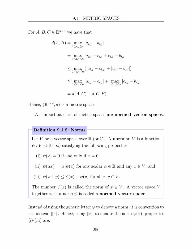
9.1. METRIC SPACES
For A,B, C ∈ Rn×n we have that
d(A,B) = max1≤i,j≤n
|ai,j − bi,j|
= max1≤i,j≤n
|ai,j − ci,j + ci,j − bi,j|
≤ max1≤i,j≤n
(|ai,j − ci,j|+ |ci,j − bi,j|)
≤ max1≤i,j≤n
|ai,j − ci,j|+ max1≤i,j≤n
|ci,j − bi,j|
= d(A,C) + d(C,B).
Hence, (Rn×n, d) is a metric space.
An important class of metric spaces are normed vector spaces.
Definition 9.1.8: Norms
Let V be a vector space over R (or C). A norm on V is a function
ψ : V → [0,∞) satisfying the following properties:
(i) ψ(x) = 0 if and only if x = 0,
(ii) ψ(αx) = |α|ψ(x) for any scalar α ∈ R and any x ∈ V , and
(iii) ψ(x+ y) ≤ ψ(x) + ψ(y) for all x, y ∈ V .
The number ψ(x) is called the norm of x ∈ V . A vector space V
together with a norm ψ is called a normed vector space.
Instead of using the generic letter ψ to denote a norm, it is convention to
use instead ‖ · ‖. Hence, using ‖x‖ to denote the norm ψ(x), properties
(i)-(iii) are:
256

9.1. METRIC SPACES
(i) ‖x‖ = 0 if and only if x = 0,
(ii) ‖αx‖ = |α| ‖x‖ for any scalar α ∈ R and any x ∈ V , and
(iii) ‖x + y‖ ≤ ‖x‖+ ‖y‖ for all x, y ∈ V .
Let (V, ‖·‖) be a normed vector space and define d : V ×V → [0,∞)
by
d(x, y) = ‖x− y‖ .
It is a straightforward exercise (which you should do) to show that
(V, d) is a metric space. Hence, every normed vector space induces a
metric space.
Example 9.1.9. The real numbers V = R form a vector space over R
under the usual operations of addition and multiplication. The absolute
value function x 7→ |x| is a norm on R. The induced metric is then
(x, y) 7→ |x− y|.
Example 9.1.10. The Euclidean norm on Rn is defined as
‖x‖2 =√
x21 + x22 + · · ·+ x2n
for x = (x1, x2, . . . , xn) ∈ Rn. It can be verified that ‖·‖2 is indeed a
norm on Rn. Hence, we define the distance between x, y ∈ Rn as
‖x− y‖2 =√
(x1 − y1)2 + (x2 − y2)2 + · · ·+ (xn − yn)2.
Notice that when n = 1, ‖·‖2 is the absolute value function since ‖x‖2 =√x2 = |x| for x ∈ R. When not specified otherwise, whenever we refer
to Rn as a normed vector space we implicitly assume that the norm is
‖·‖2 and simply use the notation ‖·‖.
257

9.1. METRIC SPACES
Example 9.1.11 (Important). The set C[a, b] of continuous functions
forms a vector space over R with addition defined as (f+g)(x) = f(x)+
g(x) for f, g ∈ C[a, b] and scalar multiplication defined as (αf)(x) =
αf(x) for α ∈ R and f ∈ C[a, b]. For f ∈ C[a, b] let
‖f‖∞ = supa≤x≤b
|f(x)| = maxa≤x≤b
|f(x)|.
It is left as an (important) exercise to show that ‖·‖∞ is indeed a norm
on C[a, b]. The induced metric is thus
d∞(f, g) = ‖f − g‖∞ = supa≤x≤b
|f(x)− g(x)|.
The norm ‖f‖∞ is called the sup-norm of f . Notice that the metric in
Example 9.1.3 is induced by the norm ‖·‖∞. Prove that (fn) converges
to f in (C[a, b], ‖·‖∞) if and only if (fn) converges uniformly to f on
[a, b].
Example 9.1.12. Two other examples of norms on C[a, b] are
‖f‖1 =∫ b
a
|f(x)| dx
and
‖f‖2 =(∫ b
a
|f(x)|2 dx)1/2
.
These norms are important in the analysis of Fourier series.
Example 9.1.13. For A ∈ Rn×n let
‖A‖∞ = max1≤i,j≤n
|ai,j|.
It is left as an exercise to show that ‖·‖∞ defined above is a norm on
Rn×n.
258

9.1. METRIC SPACES
Let (M, d) be a metric space. For x ∈M and r > 0, the open ball
centered at x of radius r is by definition the set
Br(x) = {y ∈M | d(x, y) < r}.
Example 9.1.14. Interpret geometrically the open balls in the normed
spaces (Rn, ‖·‖) for n ∈ {1, 2, 3}.
Example 9.1.15. Give a graphical/geometric description of the open
balls in the normed space (C[a, b], ‖·‖∞).
A subset S of a metric space M is called bounded if S ⊂ Br(x) for
some x ∈M and r > 0.
Example 9.1.16. Let (M, d) be a metric space. Prove that if S is
bounded then there exists y ∈ S and r > 0 such that S ⊂ Br(y).
259

9.1. METRIC SPACES
Exercises
Exercise 9.1.1. LetH be the set of all real sequences x = (x1, x2, x3, . . .)
such that |xn| ≤ 1 for all n ∈ N. For x, y ∈ H let
d(x, y) =∞∑
n=1
2−n|xn − yn|.
Prove that d is a metric on H. Note: Part of what you have to show
is that d(x, y) is well-defined.
260
9.2. SEQUENCES AND LIMITS
9.2 Sequences and Limits
Let M be a metric space. A sequence in M is a function z : N →M .
As with sequences of real numbers, we identify a sequence z : N → M
with the infinite list (zn) = (z1, z2, z3, . . .) where zn = z(n) for n ∈ N.
Definition 9.2.1: Convergence of Sequences
Let (M, d) be a metric space. A sequence (zn) in M is said to
converge if there exists p ∈M such that for any given ε > 0 there
exists K ∈ N such that d(zn, p) < ε for all n ≥ K. In this case, we
write
limn→∞
zn = p
or (zn) → p, and we call p the limit of (zn). If (zn) does not
converge then we say it is divergent.
One can indeed show, just as in Theorem 3.1.12 for sequences of real
numbers, that the point p in Definition 9.2.1 is indeed unique.
Remark 9.2.2. Suppose that (zn) converges to p and let xn = d(zn, p) ≥0. Hence, (xn) is a sequence of real numbers. If (zn) → p then for any
ε > 0 there exists K ∈ N such that xn < ε. Thus, xn = d(zn, p) → 0.
Conversely, if d(zn, p) → 0 then clearly (zn) → p.
Example 9.2.3 (Important). Prove that a sequence of continuous func-
tions (fn) on [a, b] converges uniformly on if and only if the sequence
(fn) converges in the metric space (C[a, b], ‖·‖∞).
Several of the results for sequences of real numbers carry over to
sequences on a general metric space. For example, a sequence (zn) in
M is said to be bounded if the set {zn | n ∈ N} is bounded in M .
Then:
261

9.2. SEQUENCES AND LIMITS
Lemma 9.2.4
In a metric space, a convergent sequence is bounded.
Proof. Suppose that p is the limit of (zn). There existsK ∈ N such that
d(zn, p) < 1 for all n ≥ K. Let r = 1+max{d(z1, p), . . . , d(zK−1, p)} andwe note that r ≥ 1. Then {zn | n ∈ N} ⊂ Br(p). To see this, if n ≥ K
then d(zn, p) < 1 ≤ r and thus zn ∈ Br(p). On the other hand, for zj ∈{z1, . . . , zK−1} we have that d(zj, p) ≤ max{d(z1, p), . . . , d(zK−1, p)} <r, and thus zj ∈ Br(p). This proves that (zn) is bounded.
A subsequence of a sequence (zn) is a sequence of the form (yk) =
(znk) where n1 < n2 < n3 < · · · . Then (compare with Theorem 3.4.5):
Lemma 9.2.5
LetM be a metric space and let (zn) be a sequence inM . If (zn) → p
then (znk) → p for any subsequence (znk
) of (zn).
A sequence (zn) inM is called a Cauchy sequence if for any given
ε > 0 there exists K ∈ N such that d(zn, zm) < ε for all n,m ≥ K.
Then (compare with Lemma 3.6.3-3.6.4):
Lemma 9.2.6
Let M be a metric space and let (zn) be a sequence in M . The
following hold:
(i) If (zn) is convergent then (zn) is a Cauchy sequence.
(ii) If (zn) is a Cauchy sequence then (zn) is bounded.
(iii) If (zn) is a Cauchy sequence and if (zn) has a convergent sub-
sequence then (zn) converges.
262
9.2. SEQUENCES AND LIMITS
Proof. Proofs for (i) and (ii) are left as exercises (see Lemma 3.6.3-
3.6.4). To prove (iii), let (znk) be a convergent subsequence of (zn), say
converging to p. Let ε > 0 be arbitrary. There exists K ∈ N such
that d(zn, zm) < ε/2 for all n,m ≥ K. By convergence of (znk) to p,
by increasing K if necessary we also have that d(znk, p) < ε/2 for all
k ≥ K. Therefore, if n ≥ K, then since nK ≥ K then
d(zn, p) ≤ d(zn, znK) + d(znK
, p)
< ε/2 + ε/2
= ε.
Hence, (zn) → p.
The previous lemmas (that were applicable on a general metric
space) show that some properties of sequences in R are due entirely to
the metric space structure of R. There are, however, important results
on R, most notably the Bolzano-Weierstrass theorem and the Cauchy
criterion for convergence, that do not generally carry over to a general
metric space. The Bolzano-Weierstrass theorem and the Cauchy crite-
rion rely on the completeness property of R and there is no reason to
believe that a general metric space comes equipped with a similar com-
pleteness property. Besides, the completeness axiom of R (Axiom 2.4.6)
relies on the order property of R (i.e., ≤) and there is no reason to be-
lieve that a general metric space comes equipped with an order. We
will have more to say about this in Section 9.4. For now, however, we
will consider an important metric space where almost all the results for
sequences in R carry over (an example of a result not carrying over is
the Monotone convergence theorem), namely, the normed vector space
(Rn, ‖·‖).Denoting a sequence in Rn is notationally cumbersome. Formally,
a sequence in Rn is a function z : N → Rn. How then should we
263
9.2. SEQUENCES AND LIMITS
denote z(k) as a vector in Rn? One way is to simply write z(k) =
(z1(k), z2(k), . . . , zn(k)) for each k ∈ N and this is the notation we will
adopt. It is clear that a sequence (z(k)) in Rn induces n sequences
in R, namely, (zi(k)) for each i ∈ {1, 2, . . . , n} (i.e., the component
sequences). The following theorem explains why Rn inherits almost all
the results for sequences in R.
Theorem 9.2.7: Convergence in Euclidean Spaces
Let (z(k)) = (z1(k), z2(k), . . . , zn(k)) be a sequence in the normed
vector space (Rn, ‖·‖). Then (z(k)) converges if and only if for
each i ∈ {1, 2, . . . , n} the component sequence (zi(k)) converges.
Moreover, if (z(k)) converges then
limk→∞
z(k) = ( limk→∞
z1(k), limk→∞
z2(k), . . . , limk→∞
zn(k)).
Proof. Suppose first that (z(k)) converges, say to p = (p1, p2, . . . , pn).
For any i ∈ {1, 2, . . . , n} it holds that
|zi(k)− pi| ≤√
(z1(k)− p1)2 + (z2(k)− p2)2 + · · ·+ (zn(k)− pn)2
in other words, |zi(k) − pi| ≤ ‖z(k)− p‖. Since (z(k)) → p then
limk→∞ ‖z(k)− p‖ = 0 and consequently limk→∞ |zi(k)− pi| = 0, that
is, limk→∞ zi(k) = pi.
Conversely, now suppose that (zi(k)) converges for each i ∈ {1, 2, . . . , n}.Let pi = limk→∞ zi(k) for each i ∈ {1, 2, . . . , n} and let p = (p1, p2, . . . , pn).
By the basic limit laws of sequences in R, the sequence
xk = ‖z(k)− p‖=√
(z1(k)− p1)2 + (z2(k)− p2)2 + · · ·+ (zn(k)− pn)2
converges to zero since limk→∞(zi(k) − pi)2 = 0 and the square root
function x 7→ √x is continuous. Thus, limk→∞ z(k) = p as desired.
264

9.2. SEQUENCES AND LIMITS
Corollary 9.2.8
Every Cauchy sequence in Rn is convergent.
Proof. Let (z(k)) be a Cauchy sequence in Rn. Hence, for ε > 0 there
exists K ∈ N such that ‖z(k)− z(m)‖ < ε for all k,m ≥ K. Thus, for
any i ∈ {1, 2, . . . , n}, if k,m ≥ K then
|zi(k)− zi(m)| ≤ ‖z(k)− z(m)‖ < ε.
Thus, (zi(k)) is a Cauchy sequence in R, and is therefore convergent
by the completeness property of R. By Theorem 9.2.7, this proves that
(z(k)) is convergent.
Corollary 9.2.9: Bolzano-Weierstrass in Euclidean Space
Every bounded sequence in (Rn, ‖·‖) has a convergent subsequence.
Proof. Let (z(k)) be a bounded sequence in Rn. There exists x =
(x1, . . . , xn) ∈ Rn and r > 0 such that z(k) ∈ Br(x) for all k ∈ N, that
is, ‖z(k)− x‖ < r for all k ∈ N. Therefore, for any i ∈ {1, 2 . . . , n} we
have
|zi(k)− xi| ≤ ‖z(k)− x‖ < r, ∀ k ∈ N.
This proves that (zi(k)) is a bounded sequence in R for each i ∈{1, 2, . . . , n}. We now proceed by induction. If n = 1 then (z(k)) is just
a (bounded) sequence in R and therefore, by the Bolzano-Weierstrass
theorem on R, (z(k)) has a convergent subsequence. Assume by in-
duction that for some n ≥ 1, every bounded sequence in Rn has a
convergent subsequence. Let (z(k)) be a bounded sequence in Rn+1.
Let (z(k)) be the sequence in Rn such that z(k) ∈ Rn is the vector
of the first n components of z(k) ∈ Rn+1. Then (z(k)) is a bounded
265

9.2. SEQUENCES AND LIMITS
sequence in Rn (why?). By induction, (z(k)) has a convergent subse-
quence, say it is (z(kj)). Now, the real sequence yj = zn+1(kj) ∈ R is
bounded and therefore by the Bolzano-Weierstrass theorem on R, (yj)
has a convergent subsequence which we denote by (uℓ) = (yjℓ), that
is, uℓ = zn+1(kjℓ). Now, since wℓ = z(kjℓ) is a subsequence of the con-
vergent sequence (z(kj)), (wℓ) converges in Rn. Thus, each component
of the sequence (z(kjℓ)) in Rn+1 is convergent and since (z(kjℓ)) is a
subsequence of the sequence (z(k))) the proof is complete.
A subset U of a metric space M is said to be open if for any x ∈ U
there exists ε > 0 such that Bε(x) ⊂ U . A subset E of M is closed if
Ec =M\E is open.
Example 9.2.10. Prove that an open ball Bε(x) ⊂ M is open. In
other words, prove that for each y ∈ Bε(x) there exists δ > 0 such that
Bδ(y) ⊂ Bε(x).
Example 9.2.11. Below are some facts that are easily proved; once
(a) and (b) are proved use DeMorgan’s Laws to prove (c) and (d).
(a) If U1, . . . , Un is a finite collection of open sets then⋂n
k=1Uk is
open.
(b) If {Uk} is collection of open sets indexed by a set I then⋃
k∈I Uk
is open.
(c) If E1, . . . , En is a finite collection of closed sets then⋃n
k=1Ek is
closed.
(d) If {Ek} is collection of closed sets indexed by a set I then⋂
k∈I Ek
is closed.
Below is a characterization of closed sets via sequences.
266

9.2. SEQUENCES AND LIMITS
Theorem 9.2.12: Closed Sets via Sequences
Let M be a metric space and let E ⊂ M . Then E is closed if and
only if every sequence in E that converges does so to a point in E,
that is, if (xn) → x and xn ∈ E then x ∈ E.
Proof. Suppose that E is closed and let (xn) be a sequence in E. If
x ∈ Ec then there exists ε > 0 such that Bε(x) ⊂ Ec. Hence, xn /∈Bε(x) for all n and thus (xn) does not converge to x. Hence, if (xn)
converges then it converges to a point in E. Conversely, assume that
every sequence in E that converges does so to a point in E and let
x ∈ Ec be arbitrary. Then by assumption, x is not the limit point of
any converging sequence in E. Hence, there exists ε > 0 such that
Bε(x) ⊂ Ec otherwise we can construct a sequence in E converging to
x (how?). This proves that Ec is open and thus E is closed.
Example 9.2.13. Let M be an arbitrary non-empty set and let d be
the discrete metric, that is, d(x, y) = 1 if x 6= y and d(x, y) = 0 if
x = y. Describe the converging sequences in (M, d). Prove that every
subset of M is both open and closed.
Example 9.2.14. For a ≤ b, prove that [a, b] = {x ∈ R | a ≤ x ≤ b} is
closed.
267

9.2. SEQUENCES AND LIMITS
Exercises
Exercise 9.2.1. Let M be a metric space and suppose that (zn) con-
verges in M . Prove that the limit of (zn) is unique. In other words,
prove that if p and q satisfy the convergence definition for (zn) then
p = q.
Exercise 9.2.2. Let (M, d) be a metric space.
(a) Let y ∈ M be fixed. Prove that if (zn) converges to p then
limn→∞
d(zn, y) = d(p, y).
(b) Prove that if (zn) converges to p and (yn) converges to q then
limn→∞
d(zn, yn) = d(p, q).
Exercise 9.2.3. Let M be a metric space. Prove that if U1, . . . , Un ⊂M are open then
⋂nk=1Uk is open in M .
Exercise 9.2.4. Let (M, d) be a metric space and let E ⊂M . A point
x ∈ M is called a limit point of E if there exists a sequence (xn) in
E converging to x. The closure of E, denoted by cl(E), is the union
of E and the limit points of E. If cl(E) = M then we say that E is
dense in M . As an example, Q is dense in R (why?).
(a) Let B[a, b] be the set of bounded functions on the interval [a, b],
that is f ∈ B[a, b] if and only if ‖f‖∞ < ∞. Then (B[a, b], ‖·‖∞)
is a normed vector space. Let E ⊂ B[a, b] be the set of step func-
tions on [a, b]. Prove that the set of continuous function C[a, b]
is contained in the closure of E. (Hint: See Chapter 8 in the
notes.)
(b) Perform an internet search and find dense subsets of (C[a, b], ‖·‖∞)
(you do not need to supply proofs).
268

9.2. SEQUENCES AND LIMITS
Exercise 9.2.5. For x ∈ Rn define ‖x‖∞ = max1≤i≤n |xi| and ‖x‖1 =∑n
i=1 |xi|. It is not hard to verify that these are norms on Rn. Prove
that:
(a) ‖x‖∞ ≤ ‖x‖2 ≤ ‖x‖1,
(b) ‖x‖1 ≤ n ‖x‖∞, and
(c) ‖x‖1 ≤√n ‖x‖2
Two metrics d and ρ on a set M are equivalent if they generate the
same convergent sequences, in other words, (xn) converges in (M, d) if
and only if (xn) converges in (M, ρ). Prove that ‖·‖1 , ‖·‖2 , ‖·‖∞ are
equivalent norms on Rn.
Exercise 9.2.6. Let R∞ denote the set of infinite sequences in R. It is
not hard to see that R∞ is a R-vector space with addition and scalar
multiplication defined in the obvious way. Let ℓ1 ⊂ R∞ denote the
subset of sequences x = (x1, x2, x3, . . .) such that∑∞
n=1 |xn| converges,that is, ℓ1 denotes the set of absolutely summable sequences.
(a) Prove that ℓ1 is a subspace of R∞, i.e., prove that ℓ1 is closed
under addition and scalar multiplication.
(b) For x ∈ ℓ1 let ‖x‖1 =∑∞
n=1 |xn|. Prove that ‖·‖1 defines a norm
on ℓ1.
269

9.3. CONTINUITY
9.3 Continuity
Using the definition of continuity for a function f : R → R as a guide,
it is a straightforward task to formulate a definition of continuity for a
function f : M1 → M2 where (M1, d1) and (M2, d2) are metric spaces.
Definition 9.3.1: Continuity
Let (M1, d1) and (M2, d2) be metric spaces. A function f :M1 →M2
is continuous at x ∈M1 if given any ε > 0 there exists δ > 0 such
that if d1(y, x) < δ then d2(f(y), f(x)) < ε. We say that f is
continuous if it is continuous at each point of M1.
Using open balls, f :M1 →M2 is continuous at x ∈M1 if for any given
ε > 0 there exists δ > 0 such that f(y) ∈ Bε(f(x)) whenever y ∈ Bδ(x).
We note that Bε(f(x)) is an open ball in M2 while Bδ(x) is an open
ball in M1.
Below we characterize continuity using sequences (compare with
Theorem 5.1.2).
Theorem 9.3.2: Sequential Criterion for Continuity
Let (M1, d1) and (M2, d2) be metric spaces. A function f :M1 →M2
is continuous at x ∈M1 if and only if for every sequence (xn) in M1
converging to x the sequence (f(xn)) in M2 converges to f(x).
Proof. Assume that f is continuous at x ∈ M1 and let (xn) be a se-
quence inM1 converging to x. Let ε > 0 be arbitrary. Then there exists
δ > 0 such that f(y) ∈ Bε(f(x)) for all y ∈ Bδ(x). Since (xn) → x,
there exists K ∈ N such that xn ∈ Bδ(x) for all n ≥ K. Therefore, for
270

9.3. CONTINUITY
n ≥ K we have that f(xn) ∈ Bε(f(x)). Since ε > 0 is arbitrary, this
proves that (f(xn)) converges to f(x).
Suppose that f is not continuous at x. Then there exists ε∗ > 0
such that for every δ > 0 there exists y ∈ Bδ(x) with f(y) /∈ Bε∗(f(x)).
Hence, if δn = 1n then there exists xn ∈ Bδn(x) such that f(xn) /∈
Bε∗(f(x)). Since d(xn, x) < δn then (xn) → x. On the other hand, it is
clear that (f(xn)) does not converge to f(x). Hence, if f is not contin-
uous at x then there exists a sequence (xn) converging to x such that
(f(xn)) does not converge to f(x). This proves that if every sequence
(xn) in M1 converging to x it holds that (f(xn)) converges to f(x) then
f is continuous at x.
As a consequence of Theorem 9.3.2, if f is continuous at p and limn→∞ xn =
p then limn→∞ f(xn) = f(p) can be written as
limn→∞
f(xn) = f( limn→∞
xn)
The sequential criteria for continuity can be conveniently used to show
that the composition of continuous function is a continuous function.
Lemma 9.3.3
Let f :M1 →M2 and let g :M2 →M3, where M1,M2, and M3 are
metric spaces. If f is continuous at x ∈ M1 and g is continuous at
f(x) then the composite mapping (g ◦ f) : M1 → M3 is continuous
at x ∈M1.
Proof. If limn→∞ xn = p then by Theorem 9.3.2, and using the fact that
271

9.3. CONTINUITY
f is continuous at p, and g is continuous at g(p):
(g ◦ f)(p) = g(f(p))
= g(f( limn→∞
xn))
= g( limn→∞
f(xn))
= limn→∞
g(f(xn))
= limn→∞
(g ◦ f)(xn)
In general, given functions f, g :M1 →M2 on metric spacesM1 and
M2, there is no general way to define the functions f±g or fg sinceM2
does not come equipped with a vector space structure nor is it equipped
with a product operation. However, when M2 = R then f(x) and g(x)
are real numbers which can therefore be added/subtracted/multiplied.
Proposition 9.3.4
Let (M, d) be a metric space and let f, g : M → R be continuous
functions, where R is equipped with the usual metric. If f and g
are continuous at x ∈ M then f + g, f − g, and fg are continuous
at x ∈M .
Proof. In all cases, the most economical proof is to use the sequential
criterion. The details are left as an exercise.
Recall that for any function f : A → B and S ⊂ B the set f−1(S)
is defined as
f−1(S) = {x ∈ A | f(x) ∈ S}.
272

9.3. CONTINUITY
Example 9.3.5. For any function f : A → B prove that (f−1(S))c =
f−1(Sc) for any S ⊂ B.
Proposition 9.3.6: Continuity via Open and Closed Sets
For a given function f : (M1, d1) → (M2, d2) the following are equiv-
alent:
(i) f is continuous on M1.
(ii) f−1(U) is open in M1 for every open subset U ⊂ M2.
(iii) f−1(E) is closed in M1 for every closed subset E ⊂M2.
Proof. (i) =⇒ (ii): Assume that f is continuous onM1 and let U ⊂M2
be open. Let x ∈ f−1(U) and thus f(x) ∈ U . Since U is open, there
exists ε > 0 such that Bε(f(x)) ⊂ U . By continuity of f , there exists
δ > 0 such that if y ∈ Bδ(x) then f(y) ∈ Bε(f(x)). Therefore, Bδ(x) ⊂f−1(U) and this proves that f−1(U) is open.
(ii) =⇒ (i): Let x ∈M1 and let ε > 0 be arbitrary. Since Bε(f(x)) is
open, by assumption f−1(Bε(f(x))) is open. Clearly x ∈ f−1(Bε(f(x)))
and thus there exists δ > 0 such that Bδ(x) ⊂ f−1(Bε(f(x))), in other
words, if y ∈ Bδ(x) then f(y) ∈ Bε(f(x)). This proves that f is
continuous at x.
(ii) ⇐⇒ (iii): This follows from the fact that (f−1(U))c = f−1(U c)
for any set U . Thus, for instance, if f−1(U) is open for every open set
U then if E is closed then f−1(Ec) is open, that is, (f−1(E))c is open,
i.e., f−1(E) is closed.
Example 9.3.7. A function f : (M1, d1) → (M2, d2) is called Lipschitz
on M1 if there exists K > 0 such that d2(f(x), f(y)) ≤ Kd1(x, y) for
all x, y ∈M1. Prove that a Lipschitz function is continuous.
273

9.3. CONTINUITY
Example 9.3.8. For A ∈ Rn×n recall that ‖A‖∞ = sup1≤i,j≤n |ai,j|. Lettr : Rn×n → R be the trace function on Rn×n, that is, tr(A) =
∑ni=1 ai,i.
Show that tr is Lipschitz and therefore continuous.
Let ℓ∞ denote the set of all real sequences (xn) that are bounded,
that is, {|xn| : n ∈ N} is a bounded set. If x = (xn) ∈ ℓ∞, it is
straightforward to verify that ‖x‖∞ = supn∈N |xn| defines a norm on ℓ∞with addition and scalar multiplication defined in the obvious way. Let
ℓ1 be the set of absolutely summable sequences (xn), that is, (xn) ∈ ℓ1
if and only if∑∞
n=1 |xn| converges. It is not too hard to verify that ℓ1
is a normed vector space with norm defined as ‖x‖1 =∑∞
n=1 |xn|. If∑∞
n=1 |xn| converges then (|xn|) converges to zero and thus (xn) ∈ ℓ∞,
thus ℓ1 ⊂ ℓ∞.
Example 9.3.9. Fix y = (yn)∞n=1 ∈ ℓ∞ and let h : ℓ1 → ℓ1 be defined
as h(x) = (xnyn)∞n=1 for x = (xn)
∞n=1. Verify that h is well-defined and
prove that h is continuous.
Example 9.3.10. Let det : Rn×n → R denote the determinant func-
tion. Prove that det is continuous; you may use the formula
det(A) =∑
σ∈Sn
(
sgn(σ)n∏
i=1
ai,σ(i)
)
where Sn is the set of permutations on {1, 2, . . . , n} and sgn(σ) = ±1
is the sign of the permutation σ ∈ Sn.
274
9.3. CONTINUITY
Exercises
Exercise 9.3.1. Let (M, d) be a metric space. Fix y ∈ M and define
the function f :M → R by f(x) = d(x, y). Prove that f is continuous.
Exercise 9.3.2. Let (V, ‖·‖) be a normed vector space. Prove that f :
V → R defined by f(x) = ‖x‖ is continuous. Hint: ‖a‖ ≤ ‖a− b‖+‖b‖for all a, b, c ∈ V .
Exercise 9.3.3. Consider C[a, b] with norm ‖·‖∞. Define Ψ : C[a, b] →R by Ψ(f) =
∫ b
a f(x) dx.. Prove that Ψ is continuous in two ways, using
the definition and the sequential criterion for continuity.
Exercise 9.3.4. Let M be a metric space and let f : M → R be
continuous. Prove that E = {x ∈M | f(x) = 0} is closed.
Exercise 9.3.5. Consider Rn×n as a normed vector space with norm
‖A‖∞ = sup1≤i,j≤n |ai,j| for A ∈ Rn×n.
(a) Let (A(k))∞k=1 be a sequence in Rn×n and denote the (i, j) entry
of the matrix A(k) as ai,j(k). Prove that (A(k))∞k=1 converges to
B ∈ Rn×n if and only if for all i, j ∈ {1, 2, . . . , n} the real sequence(ai,j(k))
∞k=1 converges to bi,j ∈ R.
(b) Given matrices X,Y ∈ Rn×n, recall that the entries of the prod-
uct matrix XY are (XY)i,j =∑n
ℓ=1 xi,ℓxℓ,j. Let (A(k))∞k=1 be a
sequence in Rn×n converging to B and let (C(k))∞k=1 be the se-
quence whose kth term is C(k) = A(k)A(k) = [A(k)]2. Prove
that (C(k))∞k=1 converges to B2. Hint: By part (a), it is enough
to prove that the (i, j) component of C(k) converges to the (i, j)
component of B2.
(c) Deduce that if C(k) = [A(k)]m where m ∈ N then the sequence
(C(k))∞k=1 converges to the matrix Bm.
275

9.3. CONTINUITY
(d) A polynomial matrix function is a function f : Rn×n → Rn×n
of the form
f(A) = cmAm + cm−1A
m−1 + · · ·+ c1A+ c0I
where cm, . . . , c0 are constants and I denotes the n × n identity
matrix. Prove that a polynomial matrix function is continuous.
Exercise 9.3.6. According to the sequential criterion for continuity, if
(zn) and (wn) are sequences in M converging to the same point p ∈M
and f : M → R is a function such that sequences (f(zn)) and (f(wn))
do not have the same limit f(p) (or worse one of them is divergent!)
then f is discontinuous at p. Consider f : R2 → R given by
f(x, y) =
2xyx2+y2 , (x, y) 6= (0, 0)
0, (x, y) = (0, 0).
Show that f is discontinuous at p = (0, 0).
276
9.4. COMPLETENESS
9.4 Completeness
Consider the space P [a, b] of polynomial functions on the interval [a, b].
Clearly, P [a, b] ⊂ C[a, b], and thus (P [a, b], ‖·‖∞) is a metric space. The
sequence of functions fn(x) =∑n
k=01k!xk is a sequence in P [a, b] and it
can be easily verified that (fn) converges in the metric ‖·‖∞, that is,
(fn) converges uniformly in [a, b]. However, the limiting function f is
not an element of P [a, b] because it can be verified that f ′(x) = f(x)
and the only polynomial equal to its derivative is the zero polynomial,
however, it is clear that f(0) = limn→∞ fn(0) = 1, i.e., f is not the zero
function (you may recognize, of course, that f(x) = ex). We do know,
however, that f is in C[a, b] because the uniform limit of a sequence
of continuous functions is continuous. The set P [a, b] then suffers from
the same “weakness” as do the rationals Q relative to R, namely, there
are sequences in P [a, b] that converge to elements not in P [a, b]. On the
other hand, because (fn) converges it is a Cauchy sequence in C[a, b]
and thus also in P [a, b] (the Cauchy condition only depends on the
metric) and thus (fn) is a Cauchy sequence in P [a, b] that does not
converge to an element of P [a, b]. The following discussion motivates
the following definition.
Definition 9.4.1: Complete Metric Space
A metric space M is called complete if every Cauchy sequence in
M converges in M .
This seems like a reasonable starting definition of completeness since
in R it can be proved that the Cauchy criterion (plus the Archimedean
property) implies the Completeness property of R (Theorem 3.6.8).
Based on our characterization of closed sets via sequences, we have
the following first theorem regarding completeness.
277

9.4. COMPLETENESS
Theorem 9.4.2
Let (M, d) be a complete metric space and let P ⊂M . Then (P, d)
is a complete metric space if and only if P is closed.
Proof. If (zn) is a Cauchy sequence in (P, d) then it is also a Cauchy
sequence in (M, d). Since (M, d) is complete then (zn) converges. If P
is closed then by Theorem 9.2.12 the limit of (zn) is in P . Hence, (P, d)
is a complete metric space.
Now suppose that (P, d) is a complete metric space and let (zn)
be a sequence in P that converges to z ∈ M . Then (zn) is a Cauchy
sequence in M and thus also Cauchy in P . Since P is complete then
z ∈ P . Hence, by Theorem 9.2.12 P is closed.
We now consider how to formulate the Bolzano-Weierstrass (BW)
property in a general metric space. The proof in Theorem 3.6.8 can
be easily modifield to prove that the BW property, namely that ev-
ery bounded sequence in R has a convergent subsequence, implies the
completeness property of R. We therefore want to develop a BW-type
condition in a general metric spaceM that implies thatM is complete.
Our first order of business is to develop the correct notion of bounded-
ness. We have already defined what it means for a subset E ⊂ M to
be bounded, namely, that there exists r > 0 such that E ⊂ Br(x) for
some x ∈ M . However, this notion is not enough as the next example
illustrates.
Example 9.4.3. Consider P [0, 1] with induced metric ‖·‖∞ and let
E = {f ∈ P [0, 1] : ‖f‖∞ < 3}, in other words, E is the open ball of
radius r = 3 centered at the zero function. Clearly, E is bounded and
thus any sequence in E is bounded. The sequence fn(x) =∑n
k=01k!xk
is in E, that is, ‖fn‖∞ < 3 for all n (see Example 3.3.6). However,
278

9.4. COMPLETENESS
as already discussed, (fn) converges in C[0, 1] but not to a point in
P [0, 1]. On the other hand, (fn) is a Cauchy sequence in P [0, 1] and
thus (fn) cannot have a converging subsequence in P [0, 1] by part (iii)
of Lemma 9.2.6. Thus, (fn) is a bounded sequence in P [0, 1] with no
converging subsequence in P [0, 1].
The correct notion of boundedness that is needed is the following.
Definition 9.4.4
Let (M, d) be a metric space. A subset E ⊂ M is called totally
bounded if for any given ε > 0 there exists z1, . . . , zN ∈ E such
that E ⊂ ⋃Ni=1Bε(zi).
Example 9.4.5. Prove that a subset of a totally bounded set is also
totally bounded.
Example 9.4.6. A totally bounded subset E of a metric space M is
bounded. If E ⊂ Bε(x1)∪· · ·∪Bε(xk) then if r = max2≤j≤k d(x1, xj)+ε
then if x ∈ E ∩ Bε(xj) then d(x1, x) ≤ d(x1, xj) + d(xj, x) < r. Hence,
E ⊂ Br(x1).
The following shows that the converse in the previous example does
not hold.
Example 9.4.7. Consider ℓ1 and let E = {e1, e2, e3, . . .} where ek is
the infinite sequence with entry k equal to 1 and all other entries zero.
Then ‖ek‖1 = 1 for all k ∈ N and therefore E is bounded, in particular
E ⊂ Br(0) for any r > 1. Now, ‖ek − ej‖1 = 2 for all k 6= j and thus if
ε ≤ 2 then no finite collection of open balls Bε(ek1), Bε(ek2), . . . , Bε(ekN )
can cover E. Hence, E is not totally bounded.
Example 9.4.8. Prove that a bounded subset E ofR is totally bounded.
279

9.4. COMPLETENESS
Theorem 9.4.9: Bolzano-Weierstrass
Let M be a metric space. Then M is complete if and only if every
infinite totally bounded subset of M has a limit point in M .
Proof. Suppose that (M, d) is a complete metric space. Let E be an
infinite totally bounded subset of M . Let εn = 12n for n ∈ N. For ε1
there exists z1, . . . , zm1∈ E such that E ⊂ ⋃m1
j=1Bε1(zj). Since E is
infinite, we can assume without loss of generality that E1 = E∩Bε1(z1)
contains infinitely many points of E. Let then x1 = z1. Now, E1
is totally bounded and thus there exists w1, . . . , wm2∈ E1 such that
E1 ⊂ ⋃m2
j=1Bε2(wj). Since E1 is infinite, we can assume without loss
of generality that E2 = E1 ∩ Bε2(w1) contains infinitely many points
of E1. Let x2 = w1 and therefore d(x2, x1) < ε1. Since E2 is totally
bounded there exists u1, . . . , um3∈ E2 such that E2 ⊂
⋃m3
j=1Bε3(uj). We
can assume without loss of generality that E3 = E2 ∩ Bε3(u1) contains
infinitely many elements of E2. Let x3 = u1 and thus d(x3, x2) < ε2. By
induction, there exists a sequence (xn) in E such that d(xn+1, xn) <12n .
Therefore, if m > n then by the triangle inequality (and the geometric
series) we have
d(xm, xn) ≤ d(xm, xm−1) + · · ·+ d(xn+1, xn)
<1
2m−1+ · · ·+ 1
2n
<1
2n−1.
Therefore, (xn) is a Cauchy sequence and since M is complete (xn)
converges in M . Thus E has a limit point in M .
Conversely, assume that every infinite totally bounded subset of M
has a limit point in M . Let (xn) be a Cauchy sequence in M and let
E = {xn | n ∈ N}. For any given ε > 0 there exists K ∈ N such that
280

9.4. COMPLETENESS
|xn − xK| < ε for all n ≥ K. Therefore, xn ∈ Bε(xK) for all n ≥ K
and clearly xj ∈ Bε(xj) for all j = 1, 2, . . . , K1. Thus, E is totally
bounded. By assumption, E has a limit point, that is, there exists a
subsequence of (xn) that converges inM . By part (iii) of Lemma 9.2.6,
(xn) converges in M . Thus, M is a complete metric space.
The proof in Theorem 9.4.9 that completeness implies that every
infinite totally bounded subset has a limit point is reminiscent of the
bisection method proof that a bounded sequence in R contains a con-
vergent subsequence. Also, the proof showed the following.
Lemma 9.4.10
If E is a totally bounded subset of (M, d) then E contains a Cauchy
sequence.
A complete normed vector space is usually referred to as a Banach
space in honor of Polish mathematician Stefan Banach (1892-1945)
who, in his 1920 doctorate dissertation, laid the foundations of these
spaces and their applications in integral equations. An important ex-
ample of a Banach space is the space B(M) of bounded functions from
M to R with sup-norm ‖f‖∞ = supx∈M |f(x)|. That is, for a metric
space M we set
B(M) = {f :M → R | ‖f‖∞ <∞}.
Recall that convergence in (B(M), ‖·‖∞) is uniform convergence. We
have all the tools necessary to prove that B(M) is a Banach space.
Theorem 9.4.11
The space of bounded R-valued functions on a metric space M is a
Banach space with sup-norm.
281

9.4. COMPLETENESS
Proof. First of all, it is clear that B(M) is a real vector space and thus
we need only show it is complete. The proof is essentially contained
in the Cauchy criterion for uniform convergence for functions on R
(Theorem 8.2.7). Let fn : M → R be a Cauchy sequence of bounded
functions on the metric spaceM . Then for any given ε > 0 there exists
K ∈ N such that if n,m ≥ K then ‖fn − fm‖∞ < ε. In particular, for
any fixed x ∈M it holds that
|fn(x)− fm(x)| ≤ ‖fn − fm‖∞ < ε.
Therefore, the sequence of real numbers (fn(x)) is a Cauchy sequence
and thus f(x) = limn→∞ fn(x) exists for each x ∈ M . Now, for any
fixed ε > 0, let K ∈ N be such that |fn(x)−fm(x)| < ε/2 for all x ∈M
and n,m ≥ K. Therefore, for any x ∈M we have that
limm→∞
|fn(x)− fm(x)| = |fn(x)− f(x)|≤ ε/2.
Therefore, ‖fn − f‖∞ < ε for all n ≥ K and moreover for any x ∈ M
we have
|f(x)| ≤ ‖f − fK‖∞ + ‖fK‖∞≤ ε+ ‖fK‖∞ .
This proves that f ∈ B(M) and that (fn) converges to f in (B(M), ‖·‖∞).
Corollary 9.4.12
The space of continuous functions C[a, b] on the interval [a, b] with
sup-norm is a Banach space.
282

9.4. COMPLETENESS
Proof. A continuous function on the interval [a, b] is bounded and thus
C[a, b] ⊂ B[a, b]. Convergence in B[a, b] with sup-norm is uniform con-
vergence. A sequence of continuous functions that converges uniformly
does so to a continuous functions. Hence, Theorem 9.2.12 implies that
C[a, b] is a closed subset of the complete metric space B[a, b] and then
Theorem 9.4.2 finishes the proof.
Example 9.4.13. Prove that ℓ∞ and ℓ1 are complete and hence Banach
spaces.
In a Banach space, convergence of series can be decided entirely
with the convergence of real series.
Theorem 9.4.14: Absolute Convergence Test
Let (V, ‖·‖) be a Banach space and let (zn) be a sequence in V . If the
real series∑∞
n=1 ‖zn‖ converges then the series∑∞
n=1 zn converges
in V .
Proof. Suppose that∑∞
n=1 ‖zn‖ converges, that is, suppose that the
sequence of partial sums tn =∑n
k=1 ‖zn‖ converges (note that (tn) is
increasing). By completeness of R, (tn) is a Cauchy sequence. Consider
the sequence of partial sums sn =∑n
k=1 zk. For n > m we have
‖sn − sm‖ =
∥∥∥∥∥
n∑
k=m+1
zn
∥∥∥∥∥
≤n∑
k=m+1
‖zn‖
= tn − tm
= |tn − tm|
283

9.4. COMPLETENESS
and since (tn) is Cauchy then |tn − tm| can be made arbitrarily small
provided n,m are sufficiently large. This proves that (sn) is a Cauchy
sequence in V and therefore converges since V is complete.
Remark 9.4.15. Wemake two remarks. The converse of Theorem 9.4.14
is also true, that is, if every series∑zn in (V, ‖·‖) converges whenever
∑ ‖zn‖ converges in R then V is a Banach space. Notice that the proof
of Theorem 9.4.14 is essentially the same as the proof of the Weierstrass
M -test.
Example 9.4.16. Consider the set of matrices Rn×n equipped with the
2-norm
‖A‖2 =(
n∑
i,j=1
a2i,j
)1/2
The norm ‖A‖2 is called the Frobenius norm or theHilbert-Schmidt
norm.
(a) Prove that (Rn×n, ‖·‖2) is complete.
(b) Use the Cauchy-Schwarz inequality
(N∑
ℓ=1
xℓyℓ
)2
≤(
N∑
ℓ=1
x2ℓ
)(N∑
ℓ=1
y2ℓ
)
to prove that ‖AB‖2 ≤ ‖A‖2 ‖B‖2. Conclude that∥∥Ak
∥∥2≤
(‖A‖2)k for all k ∈ N.
(c) Let f(x) =∑∞
k=1 ckxk be a power series converging on R. Define
the function f : Rn×n → Rn×n as
f(A) =
∞∑
k=1
ckAk.
284

9.4. COMPLETENESS
Prove that f is well-defined and that if ck ≥ 0 then ‖f(A)‖2 ≤f(‖A‖2), that is, that
∥∥∥∥∥
∞∑
k=1
ckAk
∥∥∥∥∥2
≤∞∑
k=1
ck ‖A‖k2
Proof. (a) The norm ‖A‖2 is simply the standard Euclidean norm on
(RN , ‖·‖2) with N = n2 and we can view matrices as elements of
RN . Hence, (Rn×n, ‖·‖2) is complete.
(b) From the Cauchy-Schwarz inequality we have
(AB)2i,j =
(n∑
ℓ=1
ai,ℓbℓ,j
)2
≤(
n∑
ℓ=1
a2i,ℓ
)(n∑
ℓ=1
b2ℓ,j
)
and therefore
‖AB‖2 =(∑
1≤i,j≤n
(AB)2i,j
)1/2
≤(∑
1≤i,j≤n
(n∑
ℓ=1
a2i,ℓ
)(n∑
ℓ=1
b2ℓ,j
))1/2
=
n∑
i,ℓ=1
a2i,ℓ
1/2
n∑
j,ℓ=1
b2ℓ,j
1/2
= ‖A‖2 ‖B‖2
(c) We first note that for any power series∑∞
k=1 akxk that converges
in (−R,R), the power series∑∞k=1 |ak|xk also converges in (−R,R).
285

9.4. COMPLETENESS
The normed space (Rn×n, ‖·‖2) is complete and thus∑∞
k=1 ckAk
converges whenever∑∞
k=1
∥∥ckA
k∥∥2converges. Now by part (b),
∥∥ckA
k∥∥2= |ck|
∥∥Ak
∥∥2≤ |ck| ‖A‖k2 and since
∑∞k=1 |ck| ‖A‖k2 con-
verges then by the comparison test for series in R, the series∑∞
k=1
∥∥ckA
k∥∥2converges. Therefore, f(A) is well-defined by The-
orem 9.4.14. To prove the last inequality, we note that the norm
function on a vector space is continuous and thus if ck ≥ 0 then
∥∥∥∥∥
m∑
k=1
ckAk
∥∥∥∥∥2
≤m∑
k=1
|ck| ‖A‖k2
≤m∑
k=1
ck ‖A‖k2
and therefore
∥∥∥∥∥
∞∑
k=1
ckAk
∥∥∥∥∥2
= limm→∞
∥∥∥∥∥
m∑
k=1
ckAk
∥∥∥∥∥2
≤ limm→∞
m∑
k=1
ck ‖A‖k2
=
∞∑
k=1
ck ‖A‖k2 ,
in other words, ‖f(A)‖2 ≤ f(‖A‖2).
Example 9.4.17. In view of the previous example, we can define for
286
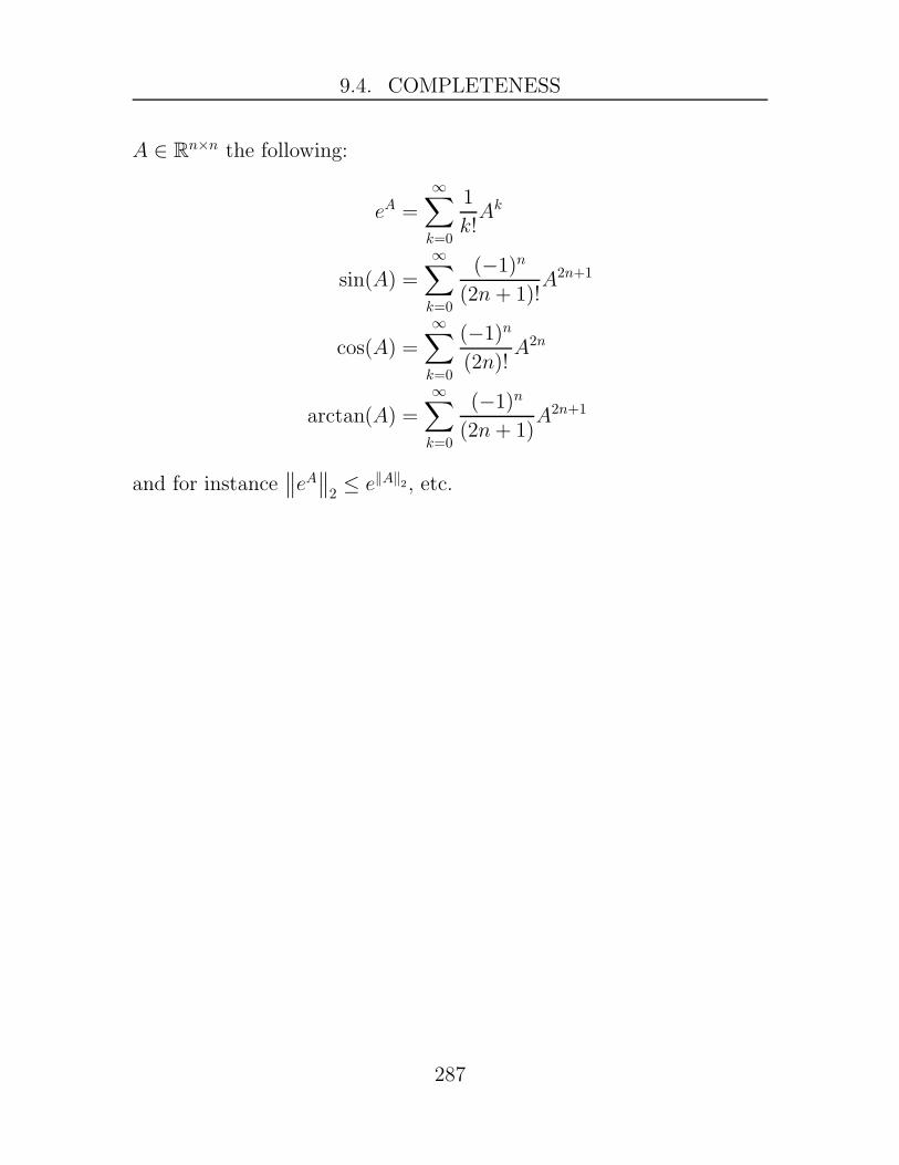
9.4. COMPLETENESS
A ∈ Rn×n the following:
eA =∞∑
k=0
1
k!Ak
sin(A) =
∞∑
k=0
(−1)n
(2n+ 1)!A2n+1
cos(A) =∞∑
k=0
(−1)n
(2n)!A2n
arctan(A) =∞∑
k=0
(−1)n
(2n+ 1)A2n+1
and for instance∥∥eA∥∥2≤ e‖A‖2, etc.
287

9.4. COMPLETENESS
Exercises
Exercise 9.4.1. Let (M1, d1) and (M2, d2) be metric spaces. There
are several ways to define a metric on the Cartesian product M1 ×M2.
One way is to imitate what was done in R2 = R × R. We can define
d :M1 ×M2 → [0,∞) as
d((x, u), (y, v)) =√
d1(x, y)2 + d2(u, v)2
(a) Prove that d is a metric on M1 ×M2.
(b) Prove that ((xn, un))∞n=1 converges in M1 × M2 if and only if
(xn)∞n=1 and (yn)
∞n=1 converge in M1 and M2, respectively.
(c) Prove that M1 ×M2 is complete if and only if M1 and M2 are
complete.
Exercise 9.4.2. Let M be a complete metric space and let (zn) be a
sequence in M such that d(zn, zn+1) < rn for all n ∈ N for some fixed
0 < r < 1. Prove that (zn) converges.
Exercise 9.4.3. Let∑∞
n=1 xn be a convergent series in a normed vector
space (V, ‖·‖) and suppose that∑∞
n=1 ‖xn‖ converges. Show that
∥∥∥∥∥
∞∑
n=1
xn
∥∥∥∥∥≤
∞∑
n=1
‖xn‖.
Note: The △-inequality can only be used on a finite sum. Hint: The
result of Exercise 9.3.2 might be useful.
288

9.5. COMPACTNESS
9.5 Compactness
Important results about continuous functions, such as the Extreme
Value Theorem (Theorem 5.3.7) and uniform continuity (Theorem 5.4.7),
depended heavily on the domain being a closed and bounded interval.
On a bounded interval, any sequence (xn) contains a Cauchy subse-
quence (xnk) (use the bisection algorithm), and if the interval is also
closed then we are guaranteed that the limit of (xnk) is contained in the
interval. We have already seen that a totally bounded subset E of a
metric space M contains a Cauchy sequence (Lemma 9.4.10) and thus
if E is complete then Cauchy sequences converge in E. This motivates
the following definition.
Definition 9.5.1: Compactness
A metric space M is called compact if M is totally bounded and
complete.
A closed and bounded subset E of R is compact. Indeed, E is complete
because it is closed (Theorem 9.4.2) and it is easy to see how to cover
E with a finite number of open intervals of any given radius ε > 0.
Conversely, if E ⊂ R is compact then E is bounded and E is closed
by Theorem 9.4.2. A similar argument shows that E ⊂ Rn is compact
if and only if E is closed and bounded. This is called the Heine-Borel
theorem.
Theorem 9.5.2: Heine-Borel
A subset E ⊂ Rn is compact if and only if E is closed and bounded.
Example 9.5.3. The unit n-sphere Sn in Rn is the set
Sn = {x = (x1, x2, . . . , xn) ∈ Rn | x21 + x22 + · · ·+ x2n = 1}.
289

9.5. COMPACTNESS
Explain why Sn is compact.
Example 9.5.4. ConsiderRn×n with norm ‖A‖2 =(∑
i,j a2i,j
)1/2
. Then
Rn×n is complete. A matrix Q ∈ Rn×n is called orthogonal if QTQ = I,
where QT denotes the transpose of Q and I is the identity matrix.
Prove that the set of orthogonal matrices, which we denote by O(n), is
compact.
A useful characterization of compactness is stated in the language
of sequences.
Theorem 9.5.5: Sequential Criterion for Compactness
A metric space M is compact if and only if every sequence in M
has a convergent subsequence.
Proof. Assume that M is compact. If (xn) is a sequence in M then
{xn | n ∈ N} is totally bounded and thus has a Cauchy subsequence
which converges by completeness of M .
Conversely, assume that every sequence inM has a convergent sub-
sequence. If (xn) is a Cauchy sequence then by assumption it has a
convergent subsequence and thus (xn) converges. This proves M is
complete. Suppose that M is not totally bounded. Then there exists
ε > 0 such that M cannot be covered by a finite number of open balls
of radius ε > 0. Hence, there exists x1, x2 ∈M such that d(x1, x2) ≥ ε.
By induction, suppose x1, . . . , xk are such that d(xi, xj) ≥ ε for i 6= j.
Then there exists xk+1 such that d(xi, xk+1) ≥ ε for all i = 1, . . . , k.
By induction then, there exists a sequence (xn) such that d(xi, xj) ≥ ε
if i 6= j. Clearly, (xn) is not a Cauchy sequence and therefore cannot
have a convergent subsequence.
Example 9.5.6. Let M be a metric space.
290

9.5. COMPACTNESS
(a) Prove that if E ⊂ M is finite then E is compact.
(b) Is the same true if E is countable?
(c) What if M is compact?
We now describe how compact sets behave under continuous func-
tions.
Theorem 9.5.7
Let f :M1 → M2 be a continuous mapping. If E ⊂ M1 is compact
then f(E) ⊂M2 is compact.
Proof. We use the sequential criterion for compactness. Let yn = f(xn)
be a sequence in f(E). Since E is compact, by Theorem 9.5.5, there is
a convergent subsequence (xnk) of (xn). By continuity of f , the subse-
quence ynk= f(xnk
) of (yn) is convergent. Hence, f(E) is compact.
We now prove a generalization of the Extreme value theorem 5.3.7.
Theorem 9.5.8: Extreme Value Theorem
Let (M, d) be a compact metric space. If f : M → R is continuous
then f achieves a maximum and a minimum on M , that is, there
exists x∗, x∗ ∈M such that f(x∗) ≤ f(x) ≤ f(x∗) for all x ∈M . In
particular, f is bounded.
Proof. By Theorem 9.5.7, f(M) is a compact subset of R and thus
f(M) is closed and bounded. Let y∗ = inf f(M) and let y∗ = sup f(M).
By the properties of the supremum, there exists a sequence (yn) in f(M)
converging to y∗. Since f(M) is closed, then y∗ ∈ f(M) and thus y∗ =
f(x∗) for some x∗ ∈M . A similar argument shows that y∗ = f(x∗) for
291

9.5. COMPACTNESS
some x∗ ∈ M . Hence, inf f(M) = f(x∗) ≤ f(x) ≤ f(x∗) = sup f(M)
for all x ∈M .
Let M be a metric space and let E ⊂ M . A cover of E is a
collection {Ui}i∈I of subsets of M whose union contains E. The index
set I may be countable or uncountable. The cover {Ui}i∈I is called an
open cover if each set Ui is open. A subcover of a cover {Ui} of E
is a cover {Uj}j∈J of E such that J ⊂ I.
Theorem 9.5.9: Compactness via Open Covers
A metric space M is compact if and only if every open cover of M
has a finite subcover.
Proof. Assume that M is compact. Then by Theorem 9.5.5, every
sequence inM has a convergent subsequence. Let {Ui} be an open cover
of M . We claim there exists ε > 0 such that for each x ∈ M it holds
that Bε(x) ⊂ Ui for some Ui. If not, then then for each n ∈ N there
exists xn ∈ M such that B1/n(xn) is not properly contained in a single
set Ui. By assumption, the sequence (xn) has a converging subsequence,
say it is (xnk) and y = limxnk
. Hence, for each k ∈ N, B1/nk(xnk
) is
not properly contained in a single Ui. Now, y ∈ Uj for some j, and
thus since Uj is open there exists δ > 0 such that Bδ(y) ⊂ Uj. Since
(xnk) → y, there exists K sufficiently large such that d(xnK
, y) < δ/2
and 1nK
< δ/2. Then B1/nK(xnK
) ⊂ Uj which is a contradiction. This
proves that such an ε > 0 exists. Now since M is totally bounded,
there exists z1, z2, . . . , zp ∈M such that Bε(z1)∪ · · ·∪Bε(zp) = M , and
since Bε(zj) ⊂ Uij for some Uij it follows that {Ui1, Ui2, . . . , Uip} is a
finite subcover of {Ui}.For the converse, we prove the contrapositive. Suppose then thatM
is not compact. Then by Theorem 9.5.5, there is a sequence (xn) in M
292

9.5. COMPACTNESS
with no convergent subsequence. In particular, there is a subsequence
(yk) of (xn) such that all yk’s are distinct and (yk) has no convergent
subsequence. Then there exists εi > 0 such that Bεi(yi) contains only
the point yi from the sequence (yk), otherwise we can construct a sub-
sequence of (yk) that converges. Hence, {Bεk(yk)}k∈N is an open cover
of the set E = {y1, y2, y3, . . . , } that has no finite subcover. The set E is
clearly closed since it consists entirely of isolated points of M . Hence,
{Bεk(yk)}k∈N∪M\E is an open cover ofM with no finite subcover.
Definition 9.5.10: Uniform Continuity
A function f : (M1, d1) → (M2, d2) is uniformly continuous if
for any ε > 0 there exists δ > 0 such that if d1(x, y) < δ then
d2(f(x), f(y)) < ε.
Example 9.5.11. A function f : (M1, d1) → (M2, d2) is Lipschitz if
there is a constant K > 0 such that d2(f(x), f(y)) ≤ Kd(x, y). Show
that a Lipschitz map is uniformly continuous.
Example 9.5.12. If f :M1 →M2 is uniformly continuous and (xn) is
a Cauchy sequence in M1, prove that (f(xn)) is a Cauchy sequence in
M2.
Theorem 9.5.13
If f : (M1, d1) → (M2, d2) is continuous and M1 is compact then f
is uniformly continuous.
Proof. Let ε > 0. For each x ∈M1, there exists rx > 0 such that if y ∈Brx(x) then f(y) ∈ Bε/2(f(x)). Now {Brx/2(x)}x∈M1
is an open cover
of M1 and since M1 is compact there exists finite x1, x2, . . . , xN such
293

9.6. FOURIER SERIES
that {Bδi(xi)}Ni=1 is an open cover of M1, where we have set δi = rxi/2.
Let δ = min{δ1, . . . , δN}. If d1(x, y) < δ, and say x ∈ Bδi(xi), then
d1(y, xi) ≤ d1(y, x) + d1(x, xi) < δ + δi < rxiand thus
d2(f(x), f(y)) ≤ d2(f(x), f(xi)) + d2(f(xi), f(y))
< ε/2 + ε/2
= ε.
This proves that f is uniformly continuous.
9.6 Fourier Series
Motivated by problems involving the conduction of heat in solids and
the motion of waves, a major problem that spurred the development of
modern analysis (and mathematics in general) was whether an arbitrary
function f can be represented by a series of the form
a02+
∞∑
n=1
(an cos(nx) + bn sin(nx))
for appropriately chosen coefficients an and bn. A central character
in this development was mathematician and physicist Joseph Fourier
and for this reason such a series is now known as a Fourier series.
Fourier made the bold claim (Theorie analytique de la Chaleur, 1822 )
that “there is no function f(x) or part of a function, which cannot be
expressed by a trigonometric series”. Fourier’s claim led B. Riemann
(1854) to develop what we now call the Riemann integral. After Rie-
mann, Cantor’s (1872) interest in trigonometric series led him to the
investigation of the derived set of a set S (which nowadays we call the
limit points of S) and he subsequently developed set theory. The gen-
eral problem of convergence of a Fourier series led to the realization that
294

9.6. FOURIER SERIES
by allowing “arbitrary” functions into the picture the theory of integra-
tion developed by Riemann would have to be extended to widened the
class of “integrable functions”. This extension of the Riemann integral
was done by Henri Lebesgue (1902) and spurred the development of
the theory of measure and integration. The Lebesgue integral is widely
accepted as the “official” integral of modern analysis.
In this section, our aim is to present a brief account of Fourier series
with the tools that we have already developed. To begin, suppose that
f : [−π, π] → R is Riemann integrable and can be represented by a
Fourier series, that is,
f(x) =a02
+∞∑
n=1
(an cos(nx) + bn sin(nx)) (9.1)
for x ∈ [−π, π]. In other words, the series on the right of (9.1) converges
pointwise to f on [−π, π]. The first question we need to answer is what
are the coefficients an and bn in terms of f? To that end, we use the
following facts. Let n,m ∈ N:
(i) For all n:∫ π
−π
sin(nx)dx =
∫ π
−π
cos(nx)dx = 0.
(ii) If n 6= m then∫ π
−π
sin(nx) sin(mx)dx =
∫ π
−π
cos(nx) cos(mx)dx = 0.
(iii) For all n and m:∫ π
−π
sin(nx) cos(mx)dx = 0.
(iv) For all n and m:∫ π
−π
sin2(nx)dx =
∫ π
−π
cos2(nx)dx = π.
295

9.6. FOURIER SERIES
Then,
∫ π
−π
f(x) cos(nx)dx =
∫ π
−π
[a02cos(nx)
+
∞∑
k=1
(ak cos(kx) cos(nx) + bk sin(kx) cos(nx))]
dx
=a02
∫ π
−π
cos(nx)dx+∞∑
k=1
ak
∫ π
−π
cos(kx) cos(nx)dx
+
∞∑
k=1
bk
∫ π
−π
sin(kx) cos(nx)dx
= anπ.
Therefore,
an =1
π
∫ π
−π
f(x) cos(nx)dx.
A similar calculation shows that
bn =1
π
∫ π
−π
f(x) sin(nx)dx.
Finally,
∫ π
−π
f(x)dx =a02
∫ π
−π
dx+∞∑
k=1
ak
∫ π
−π
cos(kx)dx+∞∑
k=1
bk
∫ π
−π
sin(kx)dx
=a022π
= a0π
and therefore
a0 =1
π
∫ π
−π
f(x)dx.
By now, you have probably noticed that these calculations are valid
provided that the Fourier series converges uniformly to f on [−π, π]
296

9.6. FOURIER SERIES
since if all we have is pointwise convergence then in general we cannot
interchange the integral sign and the infinite sum. Since the functions
fn(x) = an cos(nx) + bn sin(nx) in the Fourier series are clearly contin-
uous, and if we insist that the convergence is uniform, then we have
restricted our investigation of Fourier series to continuous functions!
Alleviating this restriction led to the development of what we now call
the Lebesgue integral; Lebesgue was interested in extending the notion
of integration beyond Riemann’s development so that a wider class of
functions could be integrated and, more importantly, this new integral
would be more robust when it came to exchanging limits with integra-
tion, i.e., uniform convergence would not be needed. We will come back
to Lebesgue and his integral, for now let’s continue with our introduc-
tion of Fourier series.
Motivated by our calculations above, suppose that f ∈ C[−π, π]and define
a0 =1
π
∫ π
−π
f(x)dx
an =1
π
∫ π
−π
f(x) cos(nx)dx
bn =1
π
∫ π
−π
f(x) sin(nx)dx.
Assume that the Fourier series of f converges uniformly on C[−π, π]and let
g(x) =a02+
∞∑
n=1
(an cos(nx) + bn sin(nx)).
Then g is continuous on [−π, π]. Does f = g? To answer this question,
our computations above show that
1
π
∫ π
−π
g(x) cos(nx)dx =1
π
∫ π
−π
f(x) cos(nx)dx
297

9.6. FOURIER SERIES
and therefore ∫ π
−π
[f(x)− g(x)] cos(nx)dx = 0
for all n ∈ N ∪ {0}. Similarly, for all n ∈ N ∪ {0} we have
∫ π
−π
[f(x)− g(x)] sin(nx)dx = 0.
Let sn(x) =a02 +
∑nk=1 ak cos(kx) + bk sin(kx) and recall that (sn) con-
verges uniformly to g. Consider for the moment
∫ π
−π
[f(x)− sn(x)]2dx =
∫ π
−π
f(x)2dx−2
∫ π
−π
f(x)sn(x)dx+
∫ π
−π
s2n(x)dx.
A straightforward computation shows that
∫ π
−π
f(x)sn(x)dx = π
[
a202+
n∑
k=1
(a2k + b2k)
]
and∫ π
−π
s2n(x)dx = π
[
a202+
n∑
k=1
(a2k + b2k)
]
.
Therefore,
1
π
∫ π
−π
[f(x)− sn(x)]2dx =
1
π
∫ π
−π
f(x)2dx− 1
π
∫ π
−π
s2n(x)dx
Now since∫ π
−π[f(x)− sn(x)]2dx ≥ 0 it follows that
1
π
∫ π
−π
s2n(x)dx ≤ 1
π
∫ π
−π
f(x)2dx,
or equivalently that
a202+
n∑
k=1
(a2k + b2k) ≤1
π
∫ π
−π
f(x)2dx.
298

9.6. FOURIER SERIES
This proves that the series a202 +
∑∞k=1(a
2k + b2k) converges and
a202+
∞∑
k=1
(a2k + b2k) ≤1
π
∫ π
−π
f(x)2dx.
In particular, limk→∞(a2k+b2k) = 0 and thus limk→∞ ak = limk→∞ bk = 0.
299

9.6. FOURIER SERIES
300

10
Multivariable Differential Calculus
In this chapter, we consider the differential calculus of mappings from
one Euclidean space to another, that is, mappings F : Rn → Rm. In
first-year calculus, you considered the case n = 2 or n = 3 and m = 1.
Examples of functions that you might have encountered were of the
type F (x1, x2) = x21 − x22, F (x1, x2, x3) = x21 + x22 + x23, or maybe even
F (x1, x2) = sin(x1) sin(x2), etc. If now F : Rn → Rm with m ≥ 2 then
F has m component functions since F (x) ∈ Rm. We can therefore
write
F (x) = (f1(x), f2(x), . . . , fm(x))
and fj : Rn → R is called the jth component of F .
In this chapter, unless stated otherwise, we equip Rn with the Eu-
clidean 2-norm ‖x‖2 =√
x21 + x22 + · · ·+ x2n. For this reason, we will
omit the subscript in ‖x‖2 and simply write ‖x‖.
10.1 Differentiation
Let U ⊂ Rn and let F : U → Rn be a function. How should we define
differentiability of F at some point a ∈ U? Recall that for a function
301

10.1. DIFFERENTIATION
f : I → R, where I ⊂ R, we say that f is differentiable at a ∈ I if
limx→a
f(x)− f(a)
x− a
exists. In this case, we denote f ′(a) = limx→af(x)−f(a)
x−a and we call f ′(a)
the derivative of f at a. As it is written, the above definition does not
make sense for F since division of vectors is not well-defined (or at least
we have not defined it). An equivalent definition of differentiability of
f at a is that there exists a number m ∈ R such that
limx→a
f(x)− f(a)−m(x− a)
x− a= 0
which is equivalent to asking that
limx→a
|f(x)− f(a)−m(x− a)||x− a| = 0.
The numberm is then denoted by m = f ′(a) as before. Another way to
think about the derivativem is that the affine function g(x) = f(a)+mx
is a good approximation to f(x) for points x near a. The linear part
of the affine function g is ℓ(x) = mx. Thought of in this way, the
derivative of f at a is a linear function.
Definition 10.1.1: The Derivative
Let U be a subset of Rn. A mapping F : U → Rm is said to be
differentiable at a ∈ U if there exists a linear mapping L : Rn →Rm such that
limx→a
‖F (x)− F (a)− L(x− a)‖‖x− a‖ = 0.
In the definition of differentiability, the expression L(x−a) denotes thelinear mapping L applied to the vector (x − a) ∈ Rn. An equivalent
302

10.1. DIFFERENTIATION
definition of differentiability is that
limh→0
‖F (x+ h)− F (a)− L(h)‖‖h‖ = 0
where again L(h) denotes h ∈ Rn evaluated at L. It is not hard to show
that the linear mapping L in the above definition is unique when U ⊂Rm is an open set. For this reason, we will deal almost exclusively with
the case that U is open without further mention. We therefore call L
the derivative of F at a and denote it instead by L = DF (a). Hence,
by definition, the derivative of F at a is the unique linear mapping
DF (a) : Rn → Rm satisfying
limx→a
‖F (x)− F (a)−DF (a)(x− a)‖‖x− a‖ = 0.
Applying the definition of the limit, given arbitrary ε > 0 there exists
δ > 0 such that if ‖x− a‖ < δ then
‖F (x)− F (a)−DF (a)(x− a)‖‖x− a‖ < ε
or equivalently
‖F (x)− F (a)−DF (a)(x− a)‖ < ε ‖x− a‖ .
If F : U → Rm is differentiable at each x ∈ U then x 7→ DF (x) is a
mapping from U to the space of linear maps from Rn to Rm. In other
words, if we denote by L(Rn;Rm) the space of linear maps from Rn to
Rm then we have a well-defined mapping DF : U → L(Rn;Rm) called
the derivative of F on U which assigns the derivative of F at each
x ∈ U .
We now relate the derivative of F with the derivatives of its com-
ponent functions. To that end, we need to recall some basic facts from
303

10.1. DIFFERENTIATION
linear algebra and the definition of the partial derivative. For the lat-
ter, recall that a function f : U ⊂ Rn → R, has partial derivative at
a ∈ U with respect to xi, if the following limit exists
limt→0
f(a1, . . . , ai−1, ai + t, ai+1, . . . , an)− f(a)
t
or equivalently, if there exists a number mi ∈ R such that
0 = limt→0
f(a+ eit)− f(a)−mit
t
where ei = (0, . . . , 0, 1, 0, . . . , 0) denotes the ith standard basis vector in
Rn. We then denote mi =∂f∂xi
(a). Now, given any linear map L : Rn →Rm, the action of L on vectors in Rn can be represented as matrix-vector
multiplication once we choose a basis for Rn and Rm. Specifically, if we
choose the most convenient bases in Rn and Rm, namely the standard
bases, then
L(x) = Ax
where A ∈ Rm×n and the the (j, i) entry of the matrix A is the jth
component of the vector Aei ∈ Rm. We can now prove the following.
304

10.1. DIFFERENTIATION
Theorem 10.1.2: Jacobian Matrix
Let U ⊂ Rn be open and suppose that F : U → Rm is differentiable
at a ∈ U , and write F = (f1, f2, . . . , fm). Then the partial deriva-
tives∂fj∂xi
(a) exist, and the matrix representation of DF (a) in the
standard bases in Rn and Rm is
∂f1∂x1
∂f1∂x2
· · · ∂f1∂xn
∂f2∂x1
∂f2∂x2
· · · ∂f2∂xn
...... . . . ...
∂fm∂x1
∂fm∂x2
· · · ∂fm∂xn
where all partial derivatives are evaluated at a. The matrix above
is called the Jacobian matrix of F at a.
Proof. Let mj,i denote the (j, i) entry of the matrix representation of
DF (a) in the standard bases in Rn and Rm, that is, mj,i is the jth
component of DF (a)ei. By definition of differentiability, it holds that
0 = limx→a
‖F (x)− F (a)−DF (a)(x− a)‖‖x− a‖ .
Let x = a+ tei where ei ∈ Rn is the ith standard basis vector. Since U
is open, x ∈ U provided t is sufficiently small. Then since ‖x− a‖ =
‖tei‖ = |t| → 0 iff ‖x− a‖ → 0 we have
0 = limt→0
‖F (a+ tei)− F (a)−DF (a)eit‖|t|
= limt→0
∥∥∥∥
1
t
[F (a+ tei)− F (a)−DF (a)eit
]∥∥∥∥.
It follows that each component of the vector 1t
[F (a + tei) − F (a) −
DF (a)eit]tends to 0 as t → 0. Hence, for each j ∈ {1, 2, . . . , m} we
305

10.1. DIFFERENTIATION
have
0 = limt→0
1
t(fj(a+ tei)− fj(a)−mj,it).
Hence,∂fj∂xi
(a) exists and mj,i =∂fj∂xi
(a) as claimed.
It is customary to write
DF (a) =
∂f1∂x1
∂f1∂x2
· · · ∂f1∂xn
∂f2∂x1
∂f2∂x2
· · · ∂f2∂xn
...... . . . ...
∂fm∂x1
∂fm∂x2
· · · ∂fm∂xn
since for any x ∈ Rn the vector DF (a)x is the Jacobian matrix of
F at a multiplied by x (all partials are evaluated at a). When not
explicitly stated, the matrix representation of DF (a) will always mean
the Jacobian matrix representation.
We now prove that differentiability implies continuity. To that end,
we first recall that if A ∈ Rm×n and B ∈ Rn×p then
‖AB‖2 ≤ ‖A‖2 ‖B‖2 .
The proof of this fact is identical to the one in Example 9.4.16. In
particular, if x ∈ Rn then ‖Ax‖2 ≤ ‖A‖2 ‖x‖.
Theorem 10.1.3: Differentiability implies Continuity
Let U ⊂ Rn be an open set. If F : U → Rm is differentiable at
a ∈ U then F is continuous at a.
Proof. Let ε1 = 1. Then there exists δ1 > 0 such that if ‖x− a‖ < δ1
then
‖F (x)− F (a)−DF (a)(x− a) +DF (a)(x− a)‖ < 1 · ‖x− a‖ .
306

10.1. DIFFERENTIATION
Then if ‖x− a‖ < δ1 then
‖F (x)− F (a)‖ = ‖F (x)− F (a)−DF (a)(x− a) +DF (a)(x− a)‖
≤ ‖F (x)− F (a)−DF (a)(x− a)‖+ ‖DF (a)(x− a)‖
≤ ‖x− a‖+ ‖DF (a)‖2 ‖x− a‖
and thus ‖F (x)− F (a)‖ < ε provided
‖x− a‖ < min{δ1, ε/(1 + ‖DF (a)‖2)}.
Hence, F is continuous at a.
Notice that Theorem 10.1.2 says that if DF (a) exists then all the
relevant partials exist. However, it does not generally hold that if all
the relevant partials exist then DF (a) exists. The reason is that partial
derivatives are derivatives along the coordinate axes whereas, as seen
from the definition, the limit used to defineDF (a) is along any direction
that x→ a.
Example 10.1.4. Consider the function f : R2 → R defined as
f(x, y) =
{2xy
x2+y2 , (x, y) 6= (0, 0)
0, (x, y) = (0, 0)
We determine whether ∂f∂x(0, 0) and ∂f
∂y(0, 0) exist. To that end, we
compute
limt→0
f(x+ t, 0)− f(0, 0)
t= lim
t→0
0
t= 0
limt→0
f(0, y + t)− f(0, 0)
t= lim
t→0
0
t= 0
307
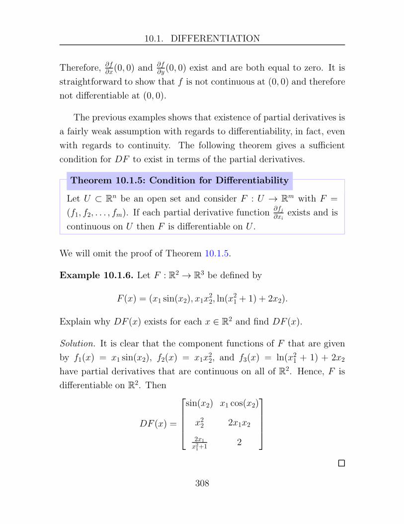
10.1. DIFFERENTIATION
Therefore, ∂f∂x(0, 0) and
∂f∂y (0, 0) exist and are both equal to zero. It is
straightforward to show that f is not continuous at (0, 0) and therefore
not differentiable at (0, 0).
The previous examples shows that existence of partial derivatives is
a fairly weak assumption with regards to differentiability, in fact, even
with regards to continuity. The following theorem gives a sufficient
condition for DF to exist in terms of the partial derivatives.
Theorem 10.1.5: Condition for Differentiability
Let U ⊂ Rn be an open set and consider F : U → Rm with F =
(f1, f2, . . . , fm). If each partial derivative function∂fj∂xi
exists and is
continuous on U then F is differentiable on U .
We will omit the proof of Theorem 10.1.5.
Example 10.1.6. Let F : R2 → R3 be defined by
F (x) = (x1 sin(x2), x1x22, ln(x
21 + 1) + 2x2).
Explain why DF (x) exists for each x ∈ R2 and find DF (x).
Solution. It is clear that the component functions of F that are given
by f1(x) = x1 sin(x2), f2(x) = x1x22, and f3(x) = ln(x21 + 1) + 2x2
have partial derivatives that are continuous on all of R2. Hence, F is
differentiable on R2. Then
DF (x) =
sin(x2) x1 cos(x2)
x22 2x1x2
2x1
x21+1
2
308
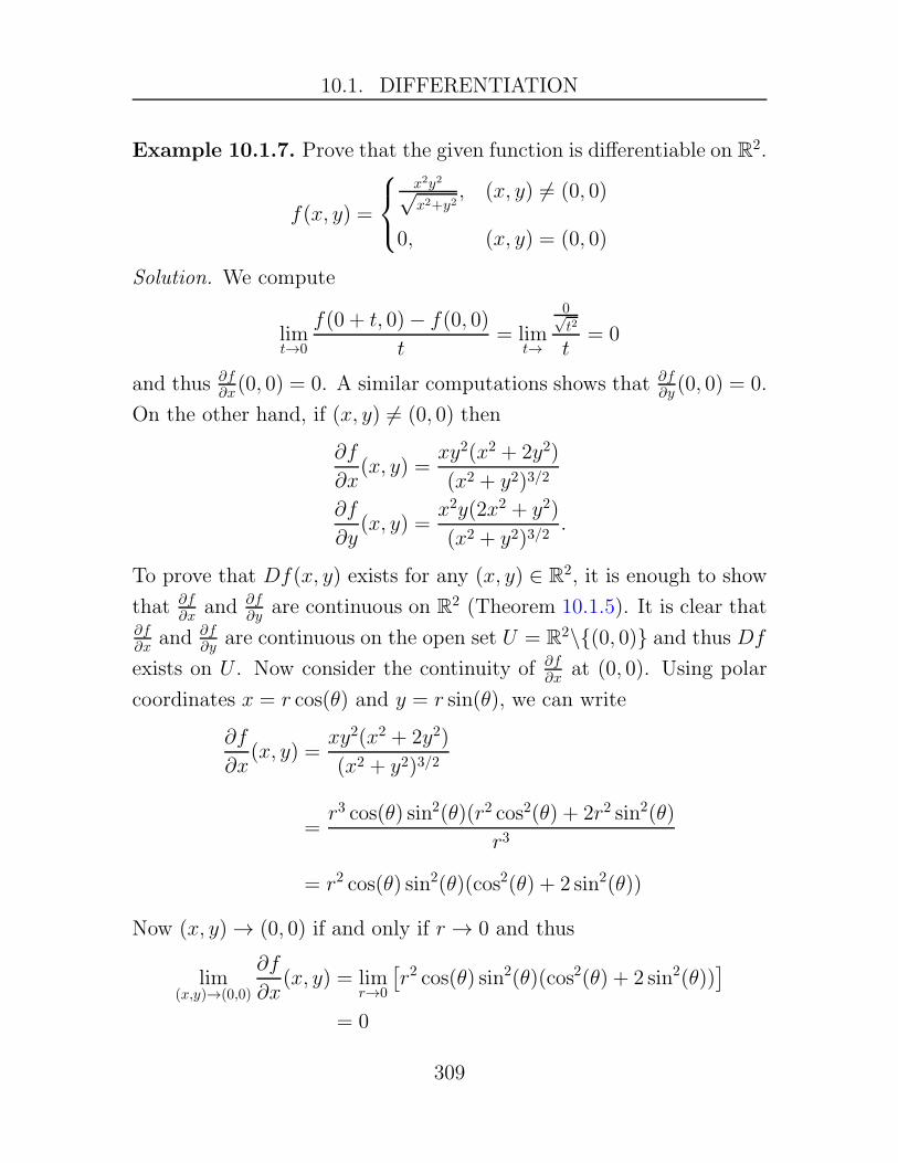
10.1. DIFFERENTIATION
Example 10.1.7. Prove that the given function is differentiable on R2.
f(x, y) =
x2y2√x2+y2
, (x, y) 6= (0, 0)
0, (x, y) = (0, 0)
Solution. We compute
limt→0
f(0 + t, 0)− f(0, 0)
t= lim
t→
0√t2
t= 0
and thus ∂f∂x(0, 0) = 0. A similar computations shows that ∂f
∂y (0, 0) = 0.
On the other hand, if (x, y) 6= (0, 0) then
∂f
∂x(x, y) =
xy2(x2 + 2y2)
(x2 + y2)3/2
∂f
∂y(x, y) =
x2y(2x2 + y2)
(x2 + y2)3/2.
To prove that Df(x, y) exists for any (x, y) ∈ R2, it is enough to show
that ∂f∂x
and ∂f∂y
are continuous on R2 (Theorem 10.1.5). It is clear that∂f∂x and ∂f
∂y are continuous on the open set U = R2\{(0, 0)} and thus Df
exists on U . Now consider the continuity of ∂f∂x
at (0, 0). Using polar
coordinates x = r cos(θ) and y = r sin(θ), we can write
∂f
∂x(x, y) =
xy2(x2 + 2y2)
(x2 + y2)3/2
=r3 cos(θ) sin2(θ)(r2 cos2(θ) + 2r2 sin2(θ)
r3
= r2 cos(θ) sin2(θ)(cos2(θ) + 2 sin2(θ))
Now (x, y) → (0, 0) if and only if r → 0 and thus
lim(x,y)→(0,0)
∂f
∂x(x, y) = lim
r→0
[r2 cos(θ) sin2(θ)(cos2(θ) + 2 sin2(θ))
]
= 0
309

10.1. DIFFERENTIATION
In other words, lim(x,y)→(0,0)∂f∂x(x, y) = ∂f
∂x(0, 0) and thus ∂f∂x is contin-
uous at (0, 0). A similar computation shows that ∂f∂y is continuous at
(0, 0). Hence, by Theorem 10.1.5, Df exists on R2.
If F : U ⊂ Rn → Rm is differentiable on U and m = 1, then DF is
called the gradient of F and we write ∇F instead of DF . Hence, in
this case,
∇F (x) =[∂F∂x1
∂F∂x2
· · · ∂F∂xn
]
On the other hand, if n = 1 and m ≥ 2 then F : U ⊂ R → Rm is
a curve in Rm. In this case, it is customary to use lower-case letters
such as c, α, or γ instead of F , and use I for the domain instead of
U . In any case, since c : I ⊂ R → Rm is a function of one variable we
use the notation c(t) = (c1(t), c2(t), . . . , cm(t)) and the derivative of c
is denoted by
dc
dt= c′(t) = (c′1(t), c
′2(t), . . . , c
′m(t))
where all derivatives are derivatives of single-variable-single-valued func-
tions.
310

10.1. DIFFERENTIATION
Exercises
Exercise 10.1.1. Let f, g : U ⊂ Rn → Rm be differentiable functions
at a ∈ U . Prove by definition that h = f + g is differentiable at a and
that Dh = Df +Dg.
Exercise 10.1.2. Recall that a mapping F : Rn → Rm is said to be
linear if F (x+y) = F (x)+F (y) and F (αx) = αF (x), for all x, y ∈ Rn
and α ∈ R. Prove that if F is linear then DF (a) = F for all a ∈ Rn.
Exercise 10.1.3. Let F : Rn → Rm and suppose that there exists
M > 0 such that ‖F (x)‖ ≤ M ‖x‖2 for all x ∈ Rn. Prove that F is
differentiable at a = 0 ∈ Rn and that DF (a) = 0.
Exercise 10.1.4. Determine if the given function is differentiable at
(x, y) = (0, 0).
f(x, y) =
xy√x2+y2
, (x, y) 6= (0, 0)
0, (x, y) = (0, 0)
Exercise 10.1.5. ComputeDF (x, y, z) if F (x, y, z) = (zxy, x2, tan(xyz)).
311

10.2. DIFFERENTIATION RULES AND THE MVT
10.2 Differentiation Rules and the MVT
Theorem 10.2.1: Chain Rule
Let U ⊂ Rn and W ⊂ Rm be open sets. Suppose that F : U → Rm
is differentiable at a, F (U) ⊂W , and G : W → Rp is differentiable
at F (a). Then (G ◦ F ) : U → Rp is differentiable at a and
D(G ◦ F )(a) = DG(F (a)) ◦DF (a)
Example 10.2.2. Verify the chain rule for the composite function H =
G ◦ F where F : R3 → R2 and G : R2 → R2 are
F (x1, x2, x3) =
[x1 − 3x2
x1x2x3
]
G(y1, y2) =
[2y1 + y2
sin(y2)
]
.
An important special case of the chain rule is the composition of a
curve γ : I ⊂ R → Rn with a function f : U ⊂ Rn → R. The composite
function f ◦ γ : I → R is a single-variable and single-valued function.
In this case, if γ ′(t) is defined for all t ∈ I and ∇f(x) exists at each
x ∈ U then
D(f ◦ γ)(t) = ∇f(γ(t)) · γ ′(t)
=[
∂f∂x1
∂f∂x2
· · · ∂f∂xn
]
γ ′1(t)γ ′2(t)...
γ ′n(t)
=
n∑
i=1
∂f
∂xi(γ(t))γ ′i(t).
312

10.2. DIFFERENTIATION RULES AND THE MVT
In the case that γ(t) = a + te and e ∈ Rn is a unit vector, that is,
‖e‖ = 1, then
limt→0
f(a+ te)− f(a)
t= D(f ◦ γ)(0)= ∇f(γ(0)) · γ ′(0)= ∇f(a) · e
is called the directional derivative of f at a in the direction
e ∈ Rn.
Example 10.2.3. Let f : R → R and F : R2 → R be differentiable and
suppose that F (x, f(x)) = 0. Prove that if ∂F∂y 6= 0 then f ′(x) = −∂F/∂x
∂F/∂y
where y = f(x).
Below is a version of the product rule for multi-variable functions.
Theorem 10.2.4: Product Rule
Let U ⊂ Rn be open and suppose that F : U → Rm and g : U → R
are differentiable at a ∈ U . Then the function G = gF : U → Rm
is differentiable at a ∈ U and
D(gF )(a) = F (a) · ∇g(a) + g(a)DF (a).
Example 10.2.5. Verify the product rule for G = gF if g : R3 → R
and F : R3 → R3 are
g(x1, x2, x3) = x21x3 − ex2
F (x1, x2, x3) =
x1x2ln(x23 + 1)
3x1 − x2 − x3
313

10.2. DIFFERENTIATION RULES AND THE MVT
Example 10.2.6. Let f, g : Rn → R be differentiable functions. Find
an expression of ∇(fg) in terms of f, g,∇f , and ∇g.
Example 10.2.7. Let f : U ⊂ Rn → R be a differentiable function.
Suppose that γ : [a, b] → Rn is differentiable. Prove that f(γ(t)) =
f(γ(a)) for all t ∈ [a, b] if and only if ∇f(γ(t)) · γ ′(t) = 0 for all
t ∈ [a, b].
Recall the mean value theorem (MVT) on R. If f : [a, b] → R
is continuous on [a, b] and differentiable on (a, b) then there exists c ∈(a, b) such that f(b)−f(a) = f ′(c)(b−a). The MVT does not generally
hold for a function F : U ⊂ Rn → Rm without some restrictions on U
and, more importantly, on m. For instance, consider f : [0, 1] → R2
defined by f(x) = (x2, x3). Then f(1)− f(0) = (1, 1)− (0, 0) = (1, 1)
while f ′(c)(1− 0) = (2c, 3c2) and there is no c ∈ R such that (1, 1) =
(2c, 3c2). With regards to the domain U , we will be able to generalize
the MVT for points a, b ∈ U provided all points on the line segment
joining a and b are contained in U . Specifically, the line segment
joining x, y ∈ U is the set of points
{z ∈ Rn | z = (1− t)x+ ty, t ∈ [0, 1]}.
Hence, the image of the curve γ : [0, 1] → Rn given by γ(t) = (1−t)x+tyis the line segment joining x and y. Even if U ⊂ Rn is open, the line
segment joining x, y ∈ U may not be contained in U (see Figure 10.1).
314

10.2. DIFFERENTIATION RULES AND THE MVT
Ux
y
Figure 10.1: Line segment joining x and y not in U
Theorem 10.2.8: Mean Value Theorem
Let U ⊂ Rn be open and assume that f : U → R is differentiable on
U . Let x, y ∈ U and suppose that the line segment joining x, y ∈ U
is contained entirely in U . Then there exists c on the line segment
joining x and y such that f(y)− f(x) = Df(c)(y − x).
Proof. Let γ(t) = (1− t)x + ty for t ∈ [0, 1]. By assumption, γ(t) ∈ U
for all 0 ≤ t ≤ 1. Consider the function h(t) = f(γ(t)) on [0, 1].
Then h is continuous on [0, 1] and by the chain rule is differentiable
on (0, 1). Hence, applying the MVT on R to h there exists t∗ ∈ (0, 1)
such that h(1)− h(0) = h′(t∗)(1− 0). Now h(0) = f(γ(0)) = f(x) and
h(1) = f(γ(1)) = f(y), and by the chain rule,
h′(t∗) = Df(γ(t∗))γ ′(t∗)
= Df(γ(t∗))(y − x).
Hence,
f(y)− f(x) = Df(γ(t∗))(y − x)
and the proof is complete.
315

10.2. DIFFERENTIATION RULES AND THE MVT
Corollary 10.2.9
Let U ⊂ Rn be open and assume that F = (f1, f2, . . . , fm) : U → Rm
is differentiable on U . Let x, y ∈ U and suppose that the line
segment joining x, y ∈ U is contained entirely in U . Then there
exists c1, c2, . . . , cm ∈ U on the line segment joining x and y such
that fi(y)− fi(x) = Dfi(ci)(y − x) for i = 1, 2, . . . , m.
Proof. Apply the MVT to each component function fi : U → R
Example 10.2.10. A set U ⊂ Rn is said to be convex if for any
x, y ∈ U the line segment joining x and y is contained in U . Let
F : U → Rm be differentiable. Prove that if U is an open convex set
and DF = 0 on U then F is constant on U .
316

10.2. DIFFERENTIATION RULES AND THE MVT
Exercises
Exercise 10.2.1. Let U ⊂ Rn be an open set satisfying the following
property: for any x, y ∈ U there is a continuous curve γ : [0, 1] → Rn
such that γ is differentiable on (0, 1) and γ(0) = x and γ(1) = y.
(a) Give an example of a non-convex set U ⊂ R2 satisfying the
above property.
(b) Prove that if U satisfies the above property and f : U → R is
differentiable on U with Df = 0 then f is constant on U .
317

10.3. HIGH-ORDER DERIVATIVES
10.3 High-Order Derivatives
In this section, we consider high-order derivatives of a differentiable
mapping F : U ⊂ Rn → Rm. To do this, we will need to make an
excursion into the world of multilinear algebra. Even though we
will discuss high-order derivatives for functions on Euclidean spaces, it
will be convenient to first work with general vector spaces.
Definition 10.3.1: Multilinear Maps
Let V1, V2, . . . , Vk andW be vector spaces. A mapping T : V1×V2×· · · × Vk → W is said to be a k-multilinear map if T is linear in
each variable separately. Specifically, for any i ∈ {1, 2, . . . , k}, andany vj ∈ Vj for j 6= i, the mapping Ti : Vi →W defined by
Ti(x) = T (v1, v2, . . . , vi−1, x, vi+1, . . . , vk)
is a linear mapping.
A 1-multilinear mapping is just a linear mapping. A 2-multilinear map-
ping is called a bilinear mapping. Hence, T : V1×V2 →W is bilinear
if
T (αu+ βv, w) = T (αu, w) + T (βv, w)
= αT (u, w) + βT (v, w)
and
T (u, αw + βy) = T (u, αw) + T (u, βy)
= αT (u, w) + βT (u, y)
318

10.3. HIGH-ORDER DERIVATIVES
for all u, v ∈ V1, w ∈ V2, and α, β ∈ R. Roughly speaking, a multi-
linear mapping is essentially a special type of polynomial multivariable
function. We will make this precise after presenting a few examples.
Example 10.3.2. Consider T : R× R → R defined as T (x, y) = 2xy.
As can be easily verified, T is bilinear. On the other hand, if T (x, y) =
x2+ y2 then T is not bilinear since for example T (αx, y) = α2x2+ y2 6=αT (x, y) in general, or T (a+ b, y) = (a+ b)2+ y2 6= T (a, y) + T (b, y) in
general. What about T (x, y) = 2xy + y3?
Example 10.3.3. Let {v1, v2, . . . , vp} be a set of vectors in Rn and
suppose that x =∑p
i=1 xivi and y =∑p
i=1 yivi. If T : Rn × Rn → Rm
is bilinear then expand T (x, y) so that it depends only on xi, yj and
T (vi, vj) for 1 ≤ i, j ≤ p.
Example 10.3.4. LetM be a n×n matrix and define T : Rn×Rn → R
as T (u, v) = uTMv. Show that T is bilinear. For instance, if say
M = [ 1 −32 1 ] then
T (u, v) = [u1 u2]
[1 −30 1
] [v1v2
]
= u1v1 − 3u1v2 + u2v2.
Notice that T (u, v) is a polynomial in the components of u and v.
Example 10.3.5. The function that returns the determinant of a ma-
trix is multilinear in the columns of the matrix. Specifically, if say
A = [a1 + b1 a2 · · · an] ∈ Rn×n then
det(A) = det([a1 a2 · · · an]) + det([b1 a2 · · · an])
and if A = [αa1 a2 · · · an] then
det(A) = α det([a1 a2 · · · an]).
319
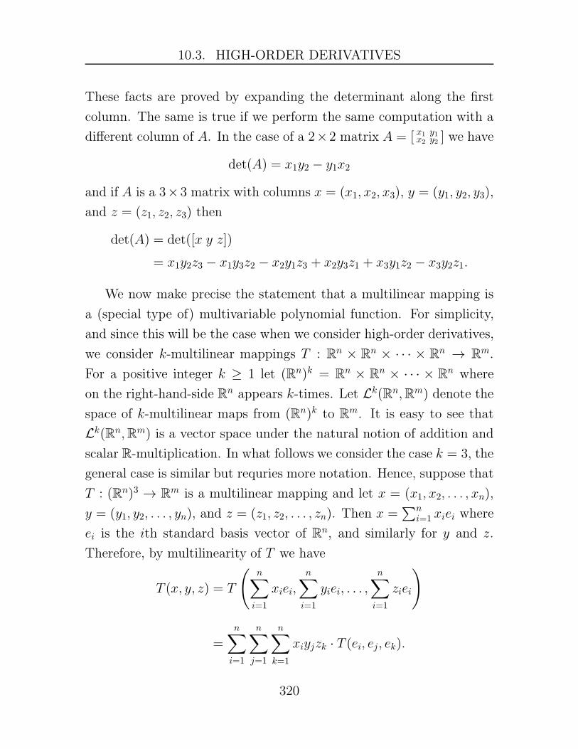
10.3. HIGH-ORDER DERIVATIVES
These facts are proved by expanding the determinant along the first
column. The same is true if we perform the same computation with a
different column of A. In the case of a 2×2 matrix A = [ x1 y1x2 y2 ] we have
det(A) = x1y2 − y1x2
and if A is a 3×3 matrix with columns x = (x1, x2, x3), y = (y1, y2, y3),
and z = (z1, z2, z3) then
det(A) = det([x y z])
= x1y2z3 − x1y3z2 − x2y1z3 + x2y3z1 + x3y1z2 − x3y2z1.
We now make precise the statement that a multilinear mapping is
a (special type of) multivariable polynomial function. For simplicity,
and since this will be the case when we consider high-order derivatives,
we consider k-multilinear mappings T : Rn × Rn × · · · × Rn → Rm.
For a positive integer k ≥ 1 let (Rn)k = Rn × Rn × · · · × Rn where
on the right-hand-side Rn appears k-times. Let Lk(Rn,Rm) denote the
space of k-multilinear maps from (Rn)k to Rm. It is easy to see that
Lk(Rn,Rm) is a vector space under the natural notion of addition and
scalar R-multiplication. In what follows we consider the case k = 3, the
general case is similar but requries more notation. Hence, suppose that
T : (Rn)3 → Rm is a multilinear mapping and let x = (x1, x2, . . . , xn),
y = (y1, y2, . . . , yn), and z = (z1, z2, . . . , zn). Then x =∑n
i=1 xiei where
ei is the ith standard basis vector of Rn, and similarly for y and z.
Therefore, by multilinearity of T we have
T (x, y, z) = T
(n∑
i=1
xiei,
n∑
i=1
yiei, . . . ,
n∑
i=1
ziei
)
=n∑
i=1
n∑
j=1
n∑
k=1
xiyjzk · T (ei, ej, ek).
320

10.3. HIGH-ORDER DERIVATIVES
Thus, to compute T (x, y, z) for any x, y, z ∈ Rn, we need only know
the values T (ei, ej, ek) ∈ Rm for all triples (i, j, k) with 1 ≤ i, j, k ≤ n.
If we set
T (ei, ej, ek) = (A1i,j,k, A
2i,j,k, . . . , A
mi,j,k)
where the superscripts are not exponents but indices, then from our
computation above
T (x, y, z) =
n∑
i,j,k=1
A1i,j,k · xiyjzk
n∑
i,j,k=1
A2i,j,k · xiyjzk...
n∑
i,j,k=1
Ami,j,k · xiyjzk
.
Notice that the component functions of T are multilinear, specifically,
the mapping
(x, y, z) 7→ Tr(x, y, z) =n∑
i,j,k=1
Ari,j,k · xiyjzk
is multilinear for each r = 1, 2, . . . , m. The n3m numbers Ari,j,k ∈ R
for 1 ≤ i, j, k ≤ n and 1 ≤ r ≤ m completely determine the multilin-
ear mapping T , and we call these the coefficients of the multilinear
mapping T in the standard bases.
Remark 10.3.6. The general case k ≥ 1 is just more notation. If T :
(Rn)k → Rm is k-multilinear then there exists nkm unique coefficients
Ari1,i2,...,ik
, where 1 ≤ i1, i2, . . . , ik ≤ n and 1 ≤ r ≤ m, such that for any
321

10.3. HIGH-ORDER DERIVATIVES
vectors u1, u2, . . . , uk ∈ Rn it holds that
T (u1, u2, . . . , uk) =
m∑
r=1
(n∑
i1=1
n∑
i2=1
· · ·n∑
ik=1
Ari1,i2,...,ik · u1,i1u2,i2 · · ·uk,ik
)
er
where e1, e2, . . . , em are the standard basis vectors in Rm.
A multilinear mapping T ∈ Lk(Rn,Rm) is said to be symmetric if
the value of T is unchanged after an arbitrary permutation of the inputs
to T . In other words, T is symmetric if for any v1, v2, . . . , vk ∈ Rn it
holds that
T (v1, v2, . . . , vk) = T (vσ(1), vσ(2), . . . , vσ(n))
for any permutation σ : {1, 2, . . . , n} → {1, 2, . . . , n}. For instance, if
T : (Rn)3 → Rm is symmetric then for any u1, u2, u3 ∈ Rn it holds that
T (u1, u2, u3) = T (u1, u3, u2)
= T (u2, u1, u3)
= T (u2, u3, u2)
= T (u3, u1, u2, )
= T (u3, u2, u1).
Example 10.3.7. Consider T : R2 × R2 → R defined by
T (x, y) = 2x1y1 + 3x1y2 + 3y1x2 − x2y2.
Then
T (y, x) = 2y1x1 + 3y1x2 + 3x1y2 − y2x2
= T (x, y)
322

10.3. HIGH-ORDER DERIVATIVES
and therefore T is symmetric. Notice that
T (x, y) = [x1 x2]
[2 33 −1
] [y1y2
]
= xTMy
and the matrix M = [ 2 33 −1 ] is symmetric.
Having introduced the very basics of multilinear mappings, we can
proceed with discussing high-order derivatives of vector-valued multi-
variable functions. Suppose then that F : U → R is differentiable on
the open set U ⊂ Rn and as usual let DF : U → L(Rn,Rm) denote
the derivative. Now L(Rn,Rm) is a finite dimensional vector space and
can be equipped with a norm (all norms on a given finite dimensional
vector space are equivalent). Thus, we can speak of differentiability
of DF , namely, DF is differentiable at a ∈ U if there exists a linear
mapping L : Rn → L(Rn,Rm) such that
limx→a
‖DF (x)−DF (a)− L(x− a)‖‖x− a‖ = 0.
If such an L exists then we denote it by L = D(DF )(a). To simplify
the notation, we write instead D(DF )(a) = D2F (a). Hence, DF is
differentiable at a ∈ U if there exists a linear mapping D2F (a) : Rn →L(Rn,Rm)) such that
limx→a
∥∥DF (x)−DF (a)−D2F (a)(x− a)
∥∥
‖x− a‖ = 0.
To say that D2F (a) is a linear mapping from Rn to L(Rn,Rm) is to say
that
D2F (a) ∈ L(Rn,L(Rn,Rm)).
323

10.3. HIGH-ORDER DERIVATIVES
Let us focus our attention on the space L(Rn,L(Rn,Rm)). If L ∈L(Rn,L(Rn,Rm)) then L(v) ∈ L(Rn,Rm) for each v ∈ Rn, and more-
over the assignment v 7→ L(v) is linear, i.e., L(αv + βu) = αL(v) +
βL(u). Now, since L(v) ∈ L(Rn,Rm), we have that
L(v)(αu+ βw) = αL(v)(u) + βL(v)(w).
In other words, the mapping
(u, v) 7→ L(u)(v)
is bilinear! Hence, L defines (uniquely) a bilinear map T : Rn × Rn →Rm by
T (u, v) = L(u)(v)
and the assignment L 7→ T is linear. Conversely, to any bilinear map
T : Rn × Rn → Rm we associate an element L ∈ L(Rn,L(Rn,Rm))
defined as
L(u)(v) = T (u, v)
and the assignment T 7→ L is linear. We have therefore proved the
following.
Lemma 10.3.8
Let V and W be vector spaces. The vector space L(V,L(V,W )) is
isomorphic to the vector space L2(V,W ) of multilinear maps from
V × V to W .
The punchline is that D2F (a) ∈ L(Rn,L(Rn,Rm)) can be viewed in
a natural way as a bilinear mapping D2F (a) : Rn×Rn → Rm and thus
from now on we write D2F (a)(u, v) instead of the more cumbersome
D2F (a)(u)(v).
324

10.3. HIGH-ORDER DERIVATIVES
We now determine a coordinate expression for D2F (a)(u, v). First
of all, if F = (f1, f2, . . . , fm) then F (x) =∑m
j=1 fj(x)ej where {e1, e2,. . . , em} is the standard basis of Rm. By linearity of the derivative and
the product rule of differentiation, we have that DF =∑m
j=1Dfj(x)ej
and also D2F =∑m
j=1D2fj(x)ej. Therefore,
D2F (a)(u, v) =m∑
j=1
D2fj(a)(u, v)ej.
This shows that we need only consider D2f for R-valued functions
f : U ⊂ Rn → R. Now,
Df =[
∂f∂x1
∂f∂x2
. . . , ∂f∂xn
]
and thus the Jacobian of Df : U → Rn is (Theorem 10.1.2)
D2f =
∂2f∂x1x1
∂2f∂x2x1
· · · ∂2f∂xnx1
∂2f∂x1x2
∂2f∂x2x2
· · · ∂2f∂xnx2
...... . . . ...
∂2f∂x1xn
∂2f∂x2xn
· · · ∂2f∂xnxn
.
Therefore,
D2f(a)(ei, ej) =∂2f
∂xjxi(a).
Therefore, for any u = (u1, u2, . . . , un) and v = (v1, v2, . . . , vn), by mul-
tilinearity we have
D2f(a)(u, v) =n∑
i=1
n∑
j=1
∂2f
∂xixj(a)uivj.
Now, if all second order partials of f are defined and continuous on U
we can say more. Let us first introduce some terminology. We say that
325

10.3. HIGH-ORDER DERIVATIVES
f : U ⊂ Rn → R is of class Ck if all partial derivatives up to and
including order k of f are continuous functions on U .
Theorem 10.3.9: Symmetry of Partial Derivatives
Let U ⊂ Rn be an open set and suppose that f : U → R is of class
C2. Then∂2f
∂xixj=
∂2f
∂xjxi
on U for all 1 ≤ i, j ≤ n. Consequently, D2f(a) is a symmetric
bilinear map on Rn × Rn.
If we now go back to a multi-valued function F : U → Rm with com-
ponents F = (f1, f2, . . . , fm), then if D2F (a) exists at a ∈ U then
D2F (a)(u, v) =
∑ni,j=1
∂2f1∂xixj
(a)uivj
∑ni,j=1
∂2f2∂xixj
(a)uivj
...
∑ni,j=1
∂2fm∂xixj
(a)uivj
Higher-order derivatives of F : U → Rm can be treated similarly. If
Dk−1F : U → Lk−1(Rn,Rm) is differentiable at a ∈ U then we denote
the derivative at a by D(Dk−1)F (a) = DkF (a). Then DkF (a) : Rn →Lk−1(Rn,Rm) is a linear map, that is,
DkF (a) ∈ L(Rn,Lk−1(Rn,Rm)).
The vector space L(Rn,Lk−1(Rn,Rm)) is isomorphic to the space of k-
multilinear maps Lk(Rn,Rm). The value of DkF (a) at u1, u2, . . . , uk ∈Rn is denoted by DkF (a)(u1, u2, . . . , uk). Moreover, DkF (a) is a sym-
metric k-multilinear map at each a ∈ U if F is of class Ck. If f : U ⊂
326

10.3. HIGH-ORDER DERIVATIVES
Rn → R is of class Ck then for vectors u1, u2, . . . , uk ∈ Rn we have
Dkf(a)(u1, u2, . . . , uk) =∑
1≤i1,i2,...,ik≤n
∂kf
∂xi1∂xi2 · · · ∂xik(a)u1,i1u2,i2 · · ·uk,ik
where the summation is over all k-tuples (i1, i2, . . . , ik) where ij ∈{1, 2, . . . , n}. Hence, there are nk terms in the above summation. In
the case that u1 = u2 = · · · = uk = x, the above expression takes the
form
Dkf(a)(x, x, . . . , x) =∑
1≤i1,i2,...,ik≤n
∂kf
∂xi1∂xi2 · · · ∂xik(a)xi1xi2 · · ·xik
Example 10.3.10. Compute D3f(a)(u, v, w) if f(x, y) = sin(x− 2y),
a = (0, 0), and u, v, w ∈ R2. Also compute D2f(a)(u, u, u).
Solution. We compute that f(0, 0) = 0 and
fx = cos(x− 2y)
fy = −2 cos(x− 2y)
and then
fxx = − sin(x− 2y)
fxy = fyx = 2 sin(x− 2y)
fyy = −4 sin(x− 2y)
and then
fxxx = − cos(x− 2y)
fyyy = 8 cos(x− 2y)
fxxy = fxyx = fyxx = 2 cos(x− 2y)
fxyy = fyxy = fyyx = −4 cos(x− 2y)
327

10.4. TAYLOR’S THEOREM
Then,
D3f(a)(u, v, w) = fxxx(a)u1v1w1 + fxxy(a)u1v1w2 + fxyx(a)u1v2w1
+ fxyy(a)u1v2w2 + fyxx(a)u2v1w1 + fyxy(a)u2v1w2
+ fyyx(a)u2v2w1 + fyyy(a)u2v2w2
= −u1v1w1 + 2u1v1w2 + 2u1v2w1 − 4u1v2w2
+ 2u2v1w1 − 4u2v1w2 − 4u2v2w1 + 8u2v2w2
= −u1v1w1 + 2(u1v1w2 + u1v2w1 + u2v1w1)
− 4(u1v2w2 + u2v1w2 + u2v2w1) + 8u2v2w2
If u = v = w then
D3f(a)(u, u, u) = −u31 + 6u21u2 − 12u1u22 + 8u32
10.4 Taylor’s Theorem
Taylor’s theorem for a function f : Rn → R is as follows.
328
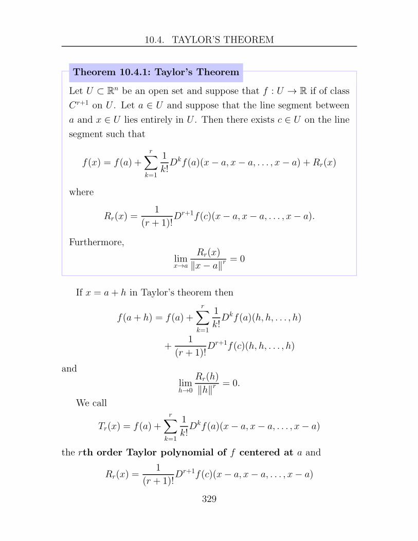
10.4. TAYLOR’S THEOREM
Theorem 10.4.1: Taylor’s Theorem
Let U ⊂ Rn be an open set and suppose that f : U → R if of class
Cr+1 on U . Let a ∈ U and suppose that the line segment between
a and x ∈ U lies entirely in U . Then there exists c ∈ U on the line
segment such that
f(x) = f(a) +r∑
k=1
1
k!Dkf(a)(x− a, x− a, . . . , x− a) +Rr(x)
where
Rr(x) =1
(r + 1)!Dr+1f(c)(x− a, x− a, . . . , x− a).
Furthermore,
limx→a
Rr(x)
‖x− a‖r = 0
If x = a+ h in Taylor’s theorem then
f(a+ h) = f(a) +
r∑
k=1
1
k!Dkf(a)(h, h, . . . , h)
+1
(r + 1)!Dr+1f(c)(h, h, . . . , h)
and
limh→0
Rr(h)
‖h‖r = 0.
We call
Tr(x) = f(a) +
r∑
k=1
1
k!Dkf(a)(x− a, x− a, . . . , x− a)
the rth order Taylor polynomial of f centered at a and
Rr(x) =1
(r + 1)!Dr+1f(c)(x− a, x− a, . . . , x− a)
329

10.4. TAYLOR’S THEOREM
the rth order remainder term. Hence, Taylor’s theorem says that
f(x) = Tr(x) + Rr(x)
Since limx→aRr(x) = 0, for x close to a we get an approximation
f(x) ≈ Tr(x).
Moreover, since Dr+1f is continuous, there is a constant M > 0 such
that if x is sufficiently close to a then the remainder term satisfies the
bound
|Rr(x)| ≤M ‖x− a‖r+1 .
From this it follows that
limx→a
Rr(x)
‖x− a‖r = 0
Example 10.4.2. Compute the third-order Taylor polynomial of f(x, y) =
sin(x− 2y) centered at a = (0, 0).
Solution. Most of the work has been done in Example 10.3.10. Evalu-
ating all derivatives at a we find that
Df(a)(u) = fx(a)u1 + fy(a)u2 = u1 − 2u2
D2f(a)(u, u) = 0
D3f(a)(u, u, u) = −u31 + 6u21u2 − 12u1u22 + 8u32
Therefore,
Tr(u) = u1 − 2u2 − u31 + 6u21u2 − 12u1u22 + 8u32.
330
10.4. TAYLOR’S THEOREM
Exercises
Exercise 10.4.1. Find the 2nd order Taylor polynomial of the function
f(x, y, z) = cos(x+ 2y)ez centered at a = (0, 0, 0).
Exercise 10.4.2. A function L : Rn → R is called a homogeneous
function of degree k ∈ N if for all α ∈ R and x ∈ Rn it holds that
L(αx) = αkL(x). Prove that if f : Rn → R is differentiable at a ∈ Rn
then the mapping
L(x) = Dkf(a)(x, x, . . . , x)
is a homogeneous function of degree k ∈ N.
331

10.5. THE INVERSE FUNCTION THEOREM
10.5 The Inverse Function Theorem
A square linear system
a1,1x1 + a1,2x2 + · · ·+ a1,nxn = y1
a2,1x1 + a2,2x2 + · · ·+ a2,nxn = y2...
... =...
an,1x1 + an,2x2 + · · ·+ an,nxn = yn
or in vector form
Ax = y,
where the unknown is x = (x1, x2, . . . , xn) ∈ Rn, has a unique solution
if and only if A−1 exists if and only if det(A) 6= 0. In this case, the
solution is y = A−1x. Another way to say this is that the mapping
F (x) = Ax has a global inverse given by F−1(x) = A−1x. Hence,
invertibility of DF = A completely determines whether F is invertible.
Consider now a system of equations
F (x) = y
where F : Rn → Rn is nonlinear. When is it possible to solve for x
in terms of y, that is, when does F−1(x) exists? In general, this is a
difficult problem and we cannot expect global invertibility even when
assuming the most desirable conditions on F . Even in the 1D case,
we cannot expect global invertibility. For instance, f(x) = cos(x) is
not globally invertible but is so on any interval where f ′(x) 6= 0. For
instance, on the interval I = (0, π), we have that f ′(x) = sin(x) 6= 0
and f−1(x) = arcsin(x). In any neighborhood where f ′(x) = 0, for
instance, at x = 0, f(x) = cos(x) is not invertible. However, having a
332

10.5. THE INVERSE FUNCTION THEOREM
non-zero derivative is not necessary for invertibility. For instance, the
function f(x) = x3 has f ′(0) = 0 but f(x) has an inverse locally around
x = 0; in fact it has a global inverse f−1(x) = x1/3.
Let’s go back to the 1D case and see if we can say something about
the invertibility of f : R → R locally about a point a such that f ′(a) 6=0. Assume that f ′ is continuous on R (or on an open set containing a).
Then there is an interval I = [a − δ, a + δ] such that f ′(x) 6= 0 for all
x ∈ I. Now if x, y ∈ I and x 6= y, then by the Mean Value Theorem,
there exists c in between x and y such that
f(y)− f(x) = f ′(c)(y − x).
Since f ′(c) 6= 0 and (y−x) 6= 0 then f(y) 6= f(x). Hence, if x 6= y then
f(y) 6= f(x) and this proves that f is injective on I = [c − δ, c + δ].
Therefore, the function f : I → R has an inverse f−1 : J → R where
J = f(I). Hence, if f(a) 6= 0, f has a local inverse at a. In fact, we
can say even more, namely, one can show that f−1 is also differentiable.
Then, since f−1(f(x)) = x for x ∈ I, by the chain rule we have
(f−1)′(f(x)) · f ′(x) = 1
and therefore since f ′(x) 6= 0 for all x ∈ I we have
(f−1)′(f(x)) =1
f ′(x).
The following theorem is a generalization of this idea.
333

10.5. THE INVERSE FUNCTION THEOREM
Theorem 10.5.1: Inverse Function Theorem
Let V ⊂ Rn be an open set and let F : V → Rn be of class C1.
Suppose that det(DF (a)) 6= 0 for a ∈ V . Then there exists an open
set U ⊂ Rn containing a such that W = F (U) is open and F : U →W is invertible. Moreover, the inverse function F−1 : W → U is
also C1 and for y ∈ W and x = F−1(y) we have
DF−1(y) = [DF (x)]−1 .
Example 10.5.2. Prove that F (x, y) = (f1(x, y), f2(x, y)) = (x2 −y2, 2xy) is locally invertible at all points a 6= (0, 0).
Proof. Clearly, DF (x, y) exists for all (x, y) since all partials of the
components of F are continuous on R2. A direct computation gives
DF (x, y) =
[2x −2y
2y 2x
]
and thus det(DF (x, y)) = 2x2+2y2. Clearly, det(DF (x, y)) = 0 if and
only if (x, y) = (0, 0). Therefore, by the Inverse Function theorem, for
each non-zero a ∈ R2 there exists an open set U ⊂ R2 containing a such
that F : U → F (U) is invertible. In this very special case, we can find
the local inverse of F about some a ∈ R2. Let (u, v) = F (x, y), that is,
x2 − y2 = u
2xy = v
If x 6= 0 then y = v2x and therefore x2− v2
4x2 = u and therefore 4x4−v2 =4ux2 or
4x4 − 4ux2 − v2 = 0.
334

10.5. THE INVERSE FUNCTION THEOREM
By the quadratic formula,
x2 =4u±
√16u2 + 16v2
8
Since x ∈ R we must take
x =
√
4u+√16u2 + 16v2
8
=
√
u+√u2 + v2
2
and therefore
y =v
2x=
√2v
2√
u+√u2 + v2
Hence, provided u 6= 0 and v 6= 0 then
F−1(u, v) =
√
u+√u2+v2
2
√2v
2√
u+√u2+v2
.
335

10.5. THE INVERSE FUNCTION THEOREM
Exercises
Exercise 10.5.1. Let F : R2 → R2 be defined by
F (x, y) = (f1(x, y), f2(x, y)) = (ex cos(y), ex sin(y))
for (x, y) ∈ R2.
(a) Prove that the range of F is R2\{0}. Hint: Think polar coordi-
nates.
(b) Prove that F is not injective.
(c) Prove that F is locally invertible at every a ∈ R2.
Exercise 10.5.2. Can the system of equations
x+ xyz = u
y + xy = v
z + 2x+ 3z2 = w
be solved for x, y, z in terms of u, v, w near (0, 0, 0)?
336