real options analysis handouts - isye homeshackman/isye6225_f09/realoptionsanalysi… · real...

REAL OPTIONS ANALYSIS HANDOUTS

1

REAL OPTION ANALYSIS EXAMPLE 1

A company is considering investing in a project. The present value (PV) of future discounted expected cash flows is either 3000 if the market goes up or 500 if the market goes down next year. The objective probability the market will go up is 20%. The appropriate risk-adjusted rate of return (cost of capital) is 25%. The initial capital investment required at time 0 is 1200. The risk-free rate is 10% per year. a. Determine the PV of the project at time 0. b. Determine the NPV of the project at time 0. c. Should the company invest in this project? d. Upon closer inspection the CFO realizes the company actually has some flexibility in managing this project. Specifically, if the market goes down, the company can abandon the project, and liquidate its original capital investment for 75% of its original value. If, however, the market should go up, the company could expand operations, which would result in twice the original PV. To expand the company will have to make an additional capital expenditure of 800. The CFO wants to know if the company should now proceed with the project with the added flexibilities, and asks for you advice. Use the original project without flexibility as the traded underlying security.

3


A company is considering investing in a project. The present value (PV) of future discounted expected cash flows is either 8000 if the market goes up or 3000 if the market goes down next year. The objective probability the market will go up is 30%. The appropriate risk-adjusted rate of return (cost of capital) is 25%. The initial capital investment required at time 0 is 4000. The risk-free rate is 5% per year. a. Determine the PV of the project without flexibility at time 0. b. Determine the NPV of the project without flexibility at time 0. c. Should the company invest in this project without flexibility? d. Suppose the company has some flexibility in managing this project. Specifically, if the market goes down, the company can abandon the project, and liquidate its original capital investment (at time 0) for 50% of its original value. If, however, the market should go up, the company could expand operations. With expansion the PV (as seen at the end of next year) will be 50% larger than the original PV forecast. To expand the company will have to make an additional capital expenditure of 1000. Using the original project without flexibility as the traded underlying security, determine the ROA value of this project with flexibility.

4


A company is considering investing in a project. The present value (PV) of future discounted expected cash flows is either 10,000 if the market goes up or 5,000 if the market goes down next year. The objective probability the market will go up is 60%. The appropriate risk-adjusted rate of return (cost of capital) is 25%. The initial capital investment required at time 0 is 8,000. The risk-free rate is 10% per year. a. Determine the PV of the project at time 0. b. Determine the NPV of the project at time 0. c. Should the company invest in this project? d. The company has some flexibility in managing this project. Specifically, if the market goes down, the company can abandon the project, and liquidate its original capital investment for 50% of its original value. If, however, the market should go up, the company could expand operations, which would result in twice the original PV. To expand the company will have to make an additional capital expenditure of 4,000. Determine the ROA value of this project with flexibility. Use the original project without flexibility as the traded underlying security. e. What is the cost of capital that will yield the correct value if the objective probabilities are used?

5

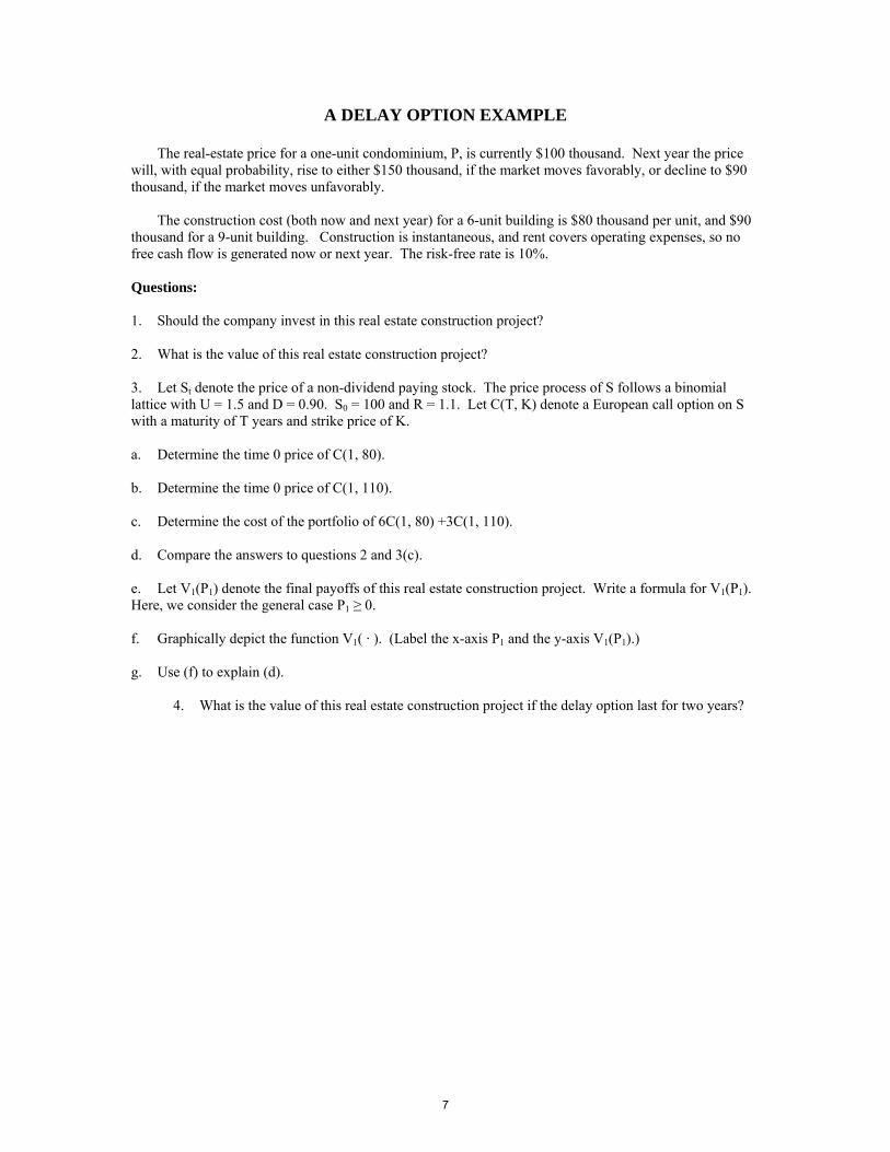
A DELAY OPTION EXAMPLE The real-estate price for a one-unit condominium, P, is currently $100 thousand. Next year the price will, with equal probability, rise to either $150 thousand, if the market moves favorably, or decline to $90 thousand, if the market moves unfavorably.

The construction cost (both now and next year) for a 6-unit building is $80 thousand per unit, and $90 thousand for a 9-unit building. Construction is instantaneous, and rent covers operating expenses, so no free cash flow is generated now or next year. The risk-free rate is 10%. Questions: 1. Should the company invest in this real estate construction project? 2. What is the value of this real estate construction project? 3. Let St denote the price of a non-dividend paying stock. The price process of S follows a binomial lattice with U = 1.5 and D = 0.90. S0 = 100 and R = 1.1. Let C(T, K) denote a European call option on S with a maturity of T years and strike price of K. a. Determine the time 0 price of C(1, 80). b. Determine the time 0 price of C(1, 110). c. Determine the cost of the portfolio of 6C(1, 80) +3C(1, 110). d. Compare the answers to questions 2 and 3(c). e. Let V1(P1) denote the final payoffs of this real estate construction project. Write a formula for V1(P1). Here, we consider the general case P1 ≥ 0. f. Graphically depict the function V1( · ). (Label the x-axis P1 and the y-axis V1(P1).) g. Use (f) to explain (d).

4. What is the value of this real estate construction project if the delay option last for two years?

7

A REDEVELOPMENT OPTION EXAMPLE

A real estate developer has the opportunity to redevelop a parcel of land over the next 5 years. Here is the relevant information:

The project is valued today at 12.5 million.

The project’s (yearly) value follows a binomial lattice with U = 1.5 and D = 2/3.

The project pays no dividends.

The cost to develop the land today is 10 million. The development cost increases 10% each year.

At the beginning of each year it costs 0.5 million to maintain the land if it is not developed for the

upcoming year. If the land is developed, then there is no maintenance cost.

During any year the developer may abandon the project and receive 1.2 million.

The objective probability of the market going up is 70%.

The risk-free rate is 10%.

The real estate developer sees this redevelopment project as a great opportunity. In fact, she is ready to develop the land today, as she has calculated its NPV at 2.5 million. She asks your consulting company for advice on what to do.

9

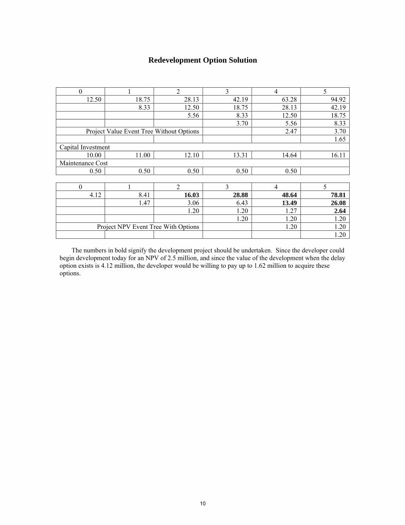
Redevelopment Option Solution

0 1 2 3 4 5 12.50 18.75 28.13 42.19 63.28 94.92

8.33 12.50 18.75 28.13 42.19 5.56 8.33 12.50 18.75 3.70 5.56 8.33

Project Value Event Tree Without Options 2.47 3.70 1.65

Capital Investment 10.00 11.00 12.10 13.31 14.64 16.11

Maintenance Cost 0.50 0.50 0.50 0.50 0.50

0 1 2 3 4 5

4.12 8.41 16.03 28.88 48.64 78.81 1.47 3.06 6.43 13.49 26.08 1.20 1.20 1.27 2.64 1.20 1.20 1.20

Project NPV Event Tree With Options 1.20 1.20 1.20

The numbers in bold signify the development project should be undertaken. Since the developer could

begin development today for an NPV of 2.5 million, and since the value of the development when the delay option exists is 4.12 million, the developer would be willing to pay up to 1.62 million to acquire these options.

10

A GROWTH OPTION EXAMPLE A biotech project involves a pioneer venture stage to first prove the new technology in order to establish its viability for future commercial development of spin-off products. The pioneer venture involves high initial costs and insufficient projected cash inflows. If the technology proves successful, subsequent product commercialization can be many times the size of the pioneer venture. Consider the following data for a particular biotech project.

• The pioneer venture requires an initial investment outlay of I0 = $100 million, and expected cash inflows over two years of C1 = $54 million and C2 = $36 million.

• The follow-on product commercialization stage will become available at the end of year two, and

its expected cash flows are 10 times the size of the pioneer venture. That is, I2 = $1,000 million, and the expected cash inflows over the subsequent two years are C3 = $540 million and C4 = $360 million.

• The cost of capital is 20% and the risk-free rate is 2.5%. (All rates are compounded annually.)

Questions: 1. Should the company invest in the pioneer venture? 2. Should the company invest in the follow-on product commercialization stage? 3. Should the company invest in this biotech project?

11

A TREE FARM EXAMPLE

You are considering an investment in a tree farm. Here are the relevant data: • Trees grow each year by the following factors:

Year 1 2 3 4 5 6 7 8 9 10 Growth 1.6 1.5 1.4 1.3 1.2 1.15 1.1 1.05 1.02 1.01

• Thus, if the initial number of trees is X, then at the end of one year there would be 1.6X trees, at the end of 2 years there would be 2.4X, etc.

• The price of lumber follows a binomial lattice with U = 1.20 and D = 0.90.

• The risk-free rate is 10%.

• It costs $2 million each year, payable at the beginning of the year, to lease the forest land.

• The initial value of the trees is $5 million (assuming they were harvested immediately).

• You can cut down the trees at the beginning of any year, collect the proceeds and not have to pay

rent after that. What is the real options value of this investment opportunity? [ROA_TreeFarmExample.hava]

13

A GOLD MINE EXAMPLE A company has the option to acquire a ten-year lease to extract gold from a gold mine. The

lease should be acquired if its cost is less than the value of the lease. Here are the relevant data:

• The mine capacity is 50,000 ounces.

• When the begin-of-year mine inventory is I, the cost to mine Q ounces for the upcoming year is 500*Q2/I.

• Production occurs instantaneously.

• Profits each year accrue at the beginning of the year.

• The price of gold follows a binomial lattice with parameters U = 1.25 and D = 0.80.

• The risk-free rate is 2.5%.

Determine the real options value of the gold mine lease. [NRA_StochasticAnalysis.01.hava and NRA_StochasticAnalysis.02.hava]

14

/** SDP.hava */ /* STOCHASTIC DYNAMIC PROGRAMMING FRAMEWORK Requires user to implement these model components: - State (of system) - Set of feasible actions for each state: sdp_ActionSet(state) - Rule that defines the sample space of events for a given state and action: sdp_GenerateSampleSpace(state, action) IMPORTANT: An event must be a struct with a required field called prob. - Rule that maps a state, action and event into next state: sdp_NextState(state, action, event) - Rule that defines immediate cash flow generated from a state and action: sdp_CashFlow(state, action) - Discount factor, which can depend on state, action and event: sdp_Discount(state, action, event) - Rule that defines the terminal condition of a state: sdp_TerminalCondition(state) - Rule that defines the terminal value of a terminal state: sdp_TerminalValue(state) - Additional (optional) information associated with each state and action (used for reporting purpose): sdp_Information(state, action) - Type of objective (maximization or minimization): sdp_Obj = sdp_MAX or sdp_MIN IMPORTANT: Default objective is sdp_MAX. A tabular display of OUTPUT is automatically generated. For each state encountered, output records: - optimal policy (optimal action, optimal value) - optional information associated with state and optimal action */

15

struct Result(policy, information); struct Policy(action, value:sdp_valueGrain); private sdp_valueGrain = 0.0001; /* Bellman Equation */ table sdp_Result(state) = if (sdp_TerminalCondition(state)) {sdp_TerminalResult(state)} else { for(a = sdp_OptAction(state)) {sdp_Result(state, a)} }; function sdp_TerminalResult(state) = Result(Policy(IGNORE, sdp_TerminalValue(state)), sdp_Information(state)); function sdp_Result(state, action) = Result(Policy(action, sdp_ExpValue(state, action)), sdp_Information(state, action)); function sdp_OptAction(state) = if (sdp_Obj == sdp_MAX) { argmax(action in sdp_ActionSet(state)) { sdp_ExpValue(state, action) } } else { argmin(action in sdp_ActionSet(state)) { sdp_ExpValue(state, action) } }; function sdp_ExpValue(state, action) = sdp_CashFlow(state, action) + sdp_ExpPresentValue(state, action):sdp_valueGrain; function sdp_ExpPresentValue(state, action) = sum(event in sdp_GenerateSampleSpace(state, action)) { sdp_Discount(state, action, event) * event.prob*sdp_Value(sdp_NextState(state, action, event)) }; function sdp_Value(state) = sdp_Result(state).policy.value:sdp_valueGrain; /* Default Values */ token sdp_MAX, sdp_MIN; function sdp_Obj = sdp_MAX; function sdp_Information(state, action) = BLANK; function sdp_Information(state) = BLANK; function sdp_TerminalValue(state) = 0;

16

/** NRA_StochasticAnalysis.01.hava */ import Lattice; import FOA_ReplicatingPortfolio; /* DATA */ /** */ r = 0.025; p0 = 400; U = 1.25; D = 0.80; dt = 1; planningHorizon = 5; I0 = 10; /** */ /* PROBLEM SPECIFICATION */ numPeriods = round(planningHorizon/dt); initialState = State(numPeriods, p0, I0); ROA_ProjectValue = sdp_Result(initialState).policy.value; /** */ import SDP_AO; /* STATE DEFINITION */ // n = number of years left in lease // p = asset price // I = inventory left in mine struct State(n, p:0.01, I); /* ACTION SET DEFINITION */ // Action = how much to produce function sdp_ActionSet(state) = 0 to state.I-1; /* NEXT STATE DEFINITION */ // nextState = one less year, new price, new inventory function sdp_NextState(state, action, event) = State(state.n-1, event.outcome, state.I-action); /* CASH FLOW DEFINITION */ // cashFlow = profit private C = 500; table sdp_CashFlow(state, action) = if (state.I == 0) {0} else {state.p*action - C*(action^2)/state.I}; /** */

17

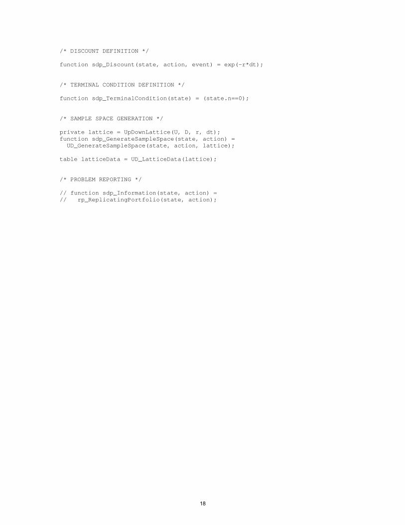
/* DISCOUNT DEFINITION */ function sdp_Discount(state, action, event) = exp(-r*dt); /* TERMINAL CONDITION DEFINITION */ function sdp_TerminalCondition(state) = (state.n==0); /* SAMPLE SPACE GENERATION */ private lattice = UpDownLattice(U, D, r, dt); function sdp_GenerateSampleSpace(state, action) = UD_GenerateSampleSpace(state, action, lattice); table latticeData = UD_LatticeData(lattice); /* PROBLEM REPORTING */ // function sdp_Information(state, action) = // rp_ReplicatingPortfolio(state, action);

18

Real Options Analysis

In these notes we show how to apply Real Options Analysis (ROA). We will develop theideas by examining five “classic” Real Options problems. We will also illustrate the potentialpitfalls of applying Decision Tree Analysis (DTA), a close companion of ROA.

1 The Delay Option

1.1 Background information

Relevant information pertaining to a project under consideration is as follows:

1. In year 1, the project’s present value (of discounted expected subsequent future) cash flowwill be 1500 if the market goes up next year and will be 666.6̄ if the market goes downnext year. The project’s present value cash flow in year 2 will be as follows: if the marketgoes up two consecutive years, then it will be 2250; if the market goes up and then downor down and then up, then it will be 1000; if the market goes down two consecutive years,then it will be 444.4̄.

2. The project pays no dividends.

3. The probability of the market going up each year is 0.70.

4. The project’s initial investment I0 (at time 0) is 1050.

5. It is possible to delay the project one year. To do so will cost the company 175 today,and the required investment next year will increase by 10%.

6. In year 1 the company can spend an additional 25 (at time 1) to delay the project onemore year. The required investment will increase by another 10%.

7. There is a tradable (non-dividend) security S whose current price is 100. Its price processfollows a binomial lattice with u = 1.5 and d = u−1 = 0.6̄.

8. The risk-free rate is 5%.

1.2 Analysis of the project without the delay option

The first step is to determine the project’s value today. The project’s payoffs P are perfectlycorrelated with the tradable security, i.e., P = 10S. Thus, the market value of P today mustbe 1000. This is the present value of the project.

19

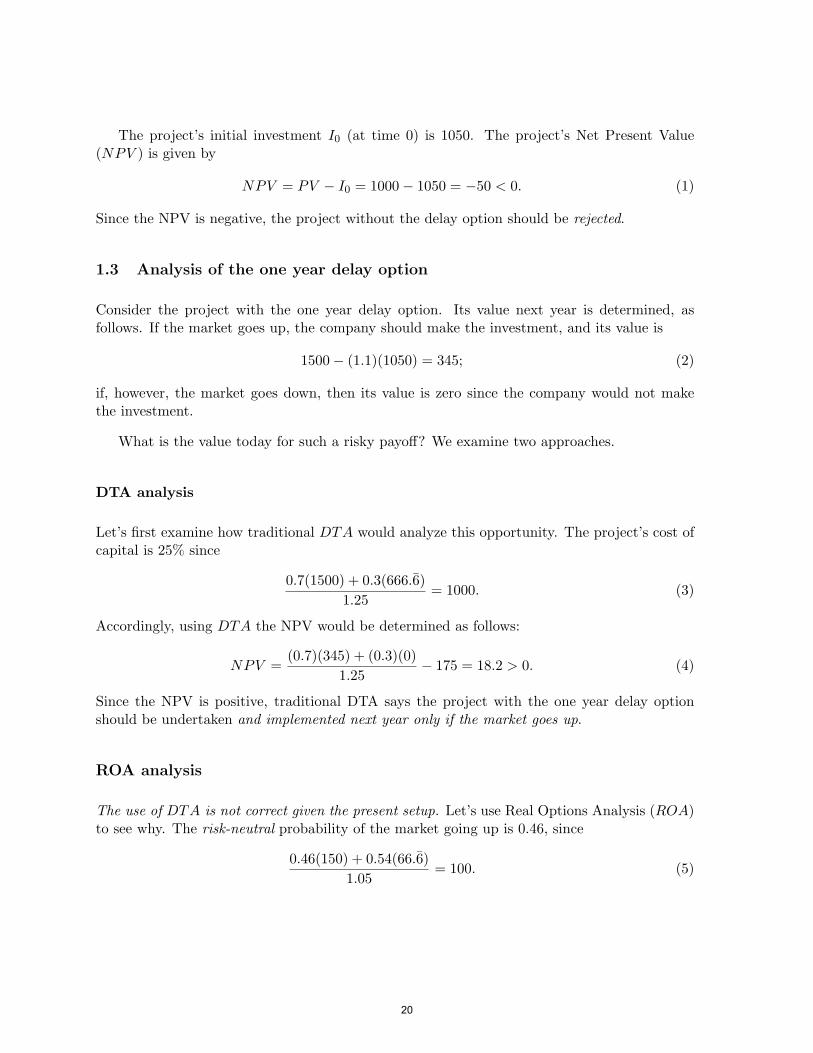
The project’s initial investment I0 (at time 0) is 1050. The project’s Net Present Value(NPV ) is given by

NPV = PV − I0 = 1000− 1050 = −50 < 0. (1)

Since the NPV is negative, the project without the delay option should be rejected.

1.3 Analysis of the one year delay option

Consider the project with the one year delay option. Its value next year is determined, asfollows. If the market goes up, the company should make the investment, and its value is

1500− (1.1)(1050) = 345; (2)

if, however, the market goes down, then its value is zero since the company would not makethe investment.

What is the value today for such a risky payoff? We examine two approaches.

DTA analysis

Let’s first examine how traditional DTA would analyze this opportunity. The project’s cost ofcapital is 25% since

0.7(1500) + 0.3(666.6̄)1.25

= 1000. (3)

Accordingly, using DTA the NPV would be determined as follows:

NPV =(0.7)(345) + (0.3)(0)

1.25− 175 = 18.2 > 0. (4)

Since the NPV is positive, traditional DTA says the project with the one year delay optionshould be undertaken and implemented next year only if the market goes up.

ROA analysis

The use of DTA is not correct given the present setup. Let’s use Real Options Analysis (ROA)to see why. The risk-neutral probability of the market going up is 0.46, since

0.46(150) + 0.54(66.6̄)1.05

= 100. (5)

20

Therefore, the correct value of the project today is computed as

0.46(345) + 0.54(0)1.05

− 175 = −23.86 < 0, (6)

and so the correct NPV says the delay option and the project should be rejected.

How can we verify/explain this? The PV of the project is 151.14 since

151.14− 175 = −23.86. (7)

Since

∆P∆S

=345− 0

150− 66.6̄= 4.14, (8)

the replicating portfolio of S and the money market M is

4.14S − 262.86M, (9)

which, not surprisingly, costs 151.14 to purchase. This portfolio’s value next year will either be345 if the market goes up or 0 if the market goes down, which exactly matches the value of theproject with the delay option.

If someone insists the correct PV is 193.2 (193.2 = 18.2 + 175), then, in principle, yousell this person a “similar” project for 193.2 and buy the replicating portfolio for 151.14. Thereplicating portfolio will fully hedge your position and you will make 193.2 − 151.14 = 42.06today, risk-free.

Remark. Using DTA can work, but only if the cost of capital is properly adjusted. Theexpected value of next year’s project value using the objective probabilities is (0.7)(345) = 241.5.Consequently, if one uses a cost of capital of 59.79%, then the PV will be 151.14, as required.As we have remarked in class, it is often difficult to arrive at correct values for the cost ofcapital at each project state since the project’s risk characteristics typically change over thelife of the project. Recall there is another way to arrive at the cost of capital of 59.79%. Thereplicating portfolio weights are

wS = 4.14(100)/151.14 = 2.739 (10)wM = −262.86/151.14 = −1.739, (11)

respectively. Since rS = 25% and rM = 5%, the replicating portfolio’s expected return is

2.739(25)− 1.739(5) = 59.79. (12)

21

Table 1: Project value event tree without flexibility

t = 0 t = 1 t = 21000 1500.00 2250.00

666.66 1000.00444.44

Sensitivity analysis

Let ρ denote the “premium” cost today to delay the project, and let 100γ% denote the percent-age increase in the required investment. As a function of ρ and γ, it is possible to determinethe acceptance region for the project.

In what follows we assume that γ > 0 and (1 + θ)(1050) < 1500. As a function of ρ and γ,the project’s correct NPV is

0.46[1500− (1 + γ)1050]1.05

− ρ, (13)

which must be positive if the project with the delay option is to be accepted. The acceptanceregion is therefore

{(γ, ρ) : 197.14 ≥ 460γ + ρ}. (14)

1.4 Analysis of the two year delay option

Project value event tree without flexibility

Table 1 records the “Project value event tree without flexibility,” which we take as our under-lying tradable security or the “twin security.”

Project value event tree with flexibility

The project with flexibility may be viewed as a collection of options on the underlying security.Table 2 records the “Project NPV event tree with flexibility” according to ROA. Here is howthese numbers were obtained.

The project will not be undertaken next year if the market goes down. We need to assessthe correct project value (with the delay options) if the market goes up. If the project is notdelayed one more year, then the project’s value is 345, as before. However, the company does

22

Table 2: Project NPV event tree with flexibility (* = delay)

t = 0 t = 1 t = 2*2.04 *404.11 979.50

0.00 0.000.00

have the option to delay one more year, and this option must be considered at this point intime. If the company chooses to delay one more year, the discounted expected project valueusing the risk-neutral probability is

0.46[1.5(1500)− (1.1)2(1050)]1.05

= 429.11. (15)

After subtracting the cost of 25 the value in this state is 404.11. Since 404.11 > 345 it isoptimal to delay the project 1 more year should the market go up next year. We conclude thatthe project’s value next year is thus 404.11 if the market goes up and 0 if the market goes down.The correct NPV for this project (with the delay options) is therefore equal to

0.46(404.11)1.05

− 175 = 2.04 > 0, (16)

and so the project with the two year delay option should be accepted.

23

2 Option to Contract Operations


A company is considering investing two projects. Relevant information is as follows:

1. Each project requires an initial investment of 80 million.

2. Each project has a present value without flexibility of 100 million.

3. Each project pays no dividends.

4. The annual volatility for the present value of project 1 is 40% (i.e. σ = 0.40) whereas theannual volatility for the present value of project 2 is 20%.

5. The appropriate cost of capital for each project is 12%.

6. The company has only 80 million to spend on new investment, so only one project maybe selected.

7. With each project it is possible to contract operations by 40% at any time during thenext two years. If operations are contracted, the salvage value (cash received) for project1 is 33 million and 42 million for project 2.


2.2 Analysis of the projects without the option to contract

Tables 3 and 4 record the respective project value event trees without flexibility. For project 1the value for u = eσ(∆t)1/2

= e0.40(1)1/2= 1.4918 (and so d = 1/u = 0.6703) and for project 2

the value for u = eσ(∆t)1/2= e0.20(1)1/2

= 1.2214 (and so d = 1/u = 0.8187).

With an initial investment of 80 million, each project has an NPV of 20 million, which ispositive. Therefore, the company should invest in one of the projects.

For subsequent reference the value event tree for each project has 6 “nodes”, which we shalllabel, respectively, as {0, U,D,UU,UD = DU,DD}.

24

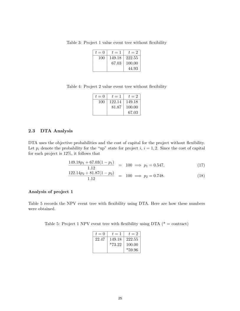
Table 3: Project 1 value event tree without flexibility

t = 0 t = 1 t = 2100 149.18 222.55

67.03 100.0044.93

Table 4: Project 2 value event tree without flexibility

t = 0 t = 1 t = 2100 122.14 149.18

81.87 100.0067.03

2.3 DTA Analysis

DTA uses the objective probabilities and the cost of capital for the project without flexibility.Let pi denote the probability for the “up” state for project i, i = 1, 2. Since the cost of capitalfor each project is 12%, it follows that

149.18p1 + 67.03(1− p1)1.12

= 100 =⇒ p1 = 0.547, (17)

122.14p2 + 81.87(1− p2)1.12

= 100 =⇒ p2 = 0.748. (18)

Analysis of project 1

Table 5 records the NPV event tree with flexibility using DTA. Here are how these numberswere obtained.

Table 5: Project 1 NPV event tree with flexibility using DTA (* = contract)

t = 0 t = 1 t = 222.47 149.18 222.55

*73.22 100.00*59.96

25

Table 6: Project 2 NPV event tree with flexibility using DTA (* = contract)

t = 0 t = 1 t = 222.36 122.58 149.18

*91.09 *102.00*82.22

We must work backwards through the value event tree. Assume the company has reachedyear 2 and has not yet exercised its option to contract. It does not pay to contract in statesUU and UD, and so their respective values remain the same at 222.55 and 100, respectively.In state DD it does pay to contact since

0.6(44.93) + 33 = 59.96 > 44.93, (19)

and so the value here is 59.96.

Now let’s move back to year 1, and suppose the company has not yet exercised its optionto contract. In state U it would not pay to contract. Now consider state D. If the companychooses to contract now, then the value would be

0.6(67.03) + 33 = 73.22. (20)

The company can, however, choose not to contract, and then the value would be

0.547(100) + 0.453(59.96)1.12

= 73.09. (21)

The best choice at state D is therefore to contract, and the associated value is 73.22.

Now let’s move back to year 0. Its value is

0.547(149.18) + 0.453(73.22)1.12

= 102.47, (22)

which gives an NPV of 102.47− 80 = 22.47.

According to DTA the option to contract is worth 2.47. Moreover, according to DTA theoption to contract should be exercised in year 1 if state D occurs.


Table 6 records the NPV event tree with flexibility using DTA. Here are how these numbersare obtained.

26

We must work backwards through the value event tree. Assume the company has reachedyear 2 and has not yet exercised its option to contract. It does not pay to contract in state UU ,and so its value remains the same at 222.55. In state UD it does pay to contact since

0.6(100) + 42 = 102 > 100, (23)

and so the value in state UD is 102. In state DD it also pays to contact since

0.6(44.93) + 42 = 82.22 > 67.03, (24)

and so the value in state DD is 82.22.

Now let’s move back to year 1, and suppose the company has not yet exercised its optionto contract. In state U it would not pay to contract. Its (new) PV is

0.748(149.18) + 0.252(102)1.12

= 122.58. (25)

Now consider state D. If the company chose to contract now, then the value would be

0.6(81.87) + 42 = 91.09. (26)

The company can, however, choose not to contract, and then the value would be

0.748(102) + 0.252(82.22)1.12

= 85.29. (27)

The best choice is therefore to contract in state D, and the associated value is 91.09.

Now let’s move back to year 0. Its value according to DTA is

0.748(122.58) + 0.252(91.09)1.12

= 102.36, (28)

which gives an NPV of 102.36− 80 = 22.36.

According to DTA the option to contract for project 2 is worth 2.36. Moreover, accordingto DTA the option to contract should be exercised in year 1 if state D occurs or in year 2 ifstate UD occurs.

Since the NPV for project 1 (2.47) is higher than that for project 2 (2.36), the companyshould invest in project 1 according to DTA.

2.4 ROA Analysis

ROA uses the risk-neutral probabilities and the risk-free rate to perform the discounted ex-pectation for valuation purposes when working backwards through the PV tree. Using ROArequires that an underlying marketable security be identified that can be used to construct thereplicating portfolio; here, we take the project without flexibility as such a security. The projectand the money complete the market, i.e., span all possible valuations on the event tree, whichthen implies risk-neutral valuation will work and provide the correct valuation.

27

Table 7: Project 1 NPV event tree with flexibility using ROA (* = contract)

t = 0 t = 1 t = 223.92 149.18 222.55

74.72 100.00*59.96


Table 7 records the Project 1 NPV event tree with flexibility using ROA. Here are how thesenumbers are obtained.

For project 1 the risk-neutral probability q1 must satisfy

149.18q1 + 67.03(1− q1)1.05

= 100 =⇒ q1 = 0.462. (29)

We now proceed, as before.

Assume the company has reached year 2 and has yet to have exercised its option to con-tract. The terminal values in year 2 are unaffected here by the change in probabilities anddiscount rate. The values for states {UU,UD,DD} are, respectively, {222.55, 100, 59.96}. (Ifthe operations have not been contracted by year 2, then the company should contract them instate DD.)

Now let’s move back to year 1, and suppose the company has not yet exercised its optionto contract. In state U it would not pay the company to contract. In this state the value willstill be

149.18 =0.462(222.55) + 0.538(100)

1.05. (30)

Now consider state D. If the company chooses to contract now, then the value would be

0.6(67.03) + 33 = 73.22, (31)

which has not changed. The company can, however, choose not to contract, and then the valueaccording to ROA would be

0.462(100) + 0.538(59.96)1.05

= 74.72. (32)

The best choice is therefore not to contract, and the associated value is 74.72. (Here is anexample of a difference between recommendations using DTA and ROA.)

28

Table 8: Project 2 NPV event tree with flexibility using ROA (* = contract)

t = 0 t = 1 t = 224.16 122.93 149.18

*91.09 *102.00*82.22

Now let’s move back to year 0. Its value according to ROA is

0.462(149.18) + 0.538(74.72)1.05

= 103.92, (33)

which gives an NPV of 103.92− 80 = 23.92. The correct value of the option to contract is 3.92for Project 1. The company should only contract operations if it reaches state DD in year 2.


Table 8 records the Project 2 NPV event tree with flexibility using ROA. Here are how thesenumbers are obtained.

For project 2 the risk-neutral probability q2 must satisfy

122.14q2 + 81.87(1− q2)1.05

= 100 =⇒ q2 = 0.574. (34)

We now proceed, as before.

Assume the company has reached year 2 and has not yet exercised its option to contract. Theterminal values in year 2 are unaffected here by the change in probabilities and discount rate.The values for states {UU,UD,DD} are, respectively, {149.18, 102, 82.22}. (If the companyhas not contacted operations by year 2, then it should contract them if either state UD or DD.)

Now let’s move back to year 1, and suppose the company has not yet exercised its option tocontract. In state U it would not pay the company to contract. In this state the value will be

0.574(149.18) + 0.426(102)1.05

= 122.93. (35)

(This value will change since the value for state UD changed.) Now consider state D. If thecompany chooses to contract now, then the value would be

0.6(81.87) + 42 = 91.09, (36)

29

which has not changed. The company can, however, choose not to contract, and then the valueaccording to ROA would be

0.574(102) + 0.426(82.22)1.05

= 89.12. (37)

The best choice is therefore to contract, and the associated value is still 91.09.

Now let’s move back to year 0. Its value according to ROA is

0.574(122.93) + 0.426(91.09)1.05

= 104.16, (38)

which gives an NPV of 104.16− 80 = 24.16. The correct value of the option to contract is 4.16for Project 2. The company should contract operations if it reaches state D in year 1.

2.5 Comparison of DTA to ROA

DTA recommends Project 1 since 22.47 > 22.36, whereas ROA recommends Project 2 since24.16 > 23.92. (They are close.) The optimal contract policy changes, too.

30


t = 0 t = 1 t = 2 t = 3100 134.99 182.21 245.96

74.08 100.00 134.9954.88 74.08

40.66

3 Option to Abandon Operations


A company is considering investing in a project. Relevant information is as follows:

1. The project’s present value without flexibility is 100 million.

2. The project pays no dividends.

3. The project’s present value without flexibility has an annual volatility of 30%.

4. The project requires an initial investment of 108 million.

5. The appropriate cost of capital for the project is 15%.

6. The company has the option to abandon operations at any time during the next 3 years,and receive an after-tax cash flow (salvage value) of 90 million.


3.2 Analysis of project without flexibility

The project’s NPV is 100 − 108 = −8 < 0, and so this the company should not invest in theproject without flexibility.

For subsequent reference Table 9 records the Project value event tree for the project with-out flexibility. It has 10 “nodes”, which we shall label, respectively, as {0, U,D,UU,UD =DU,DD,UUU,UUD = UDU = DUU,UDD = DUD = DDU,DDD}. The value for u ise0.30 = 1.3499 and d is e−0.30 = 0.7408.

31

Table 10: Project NPV event tree with flexibility using DTA (* = abandon)

t = 0 t = 1 t = 2 t = 3-2.69 136.29 182.21 245.96

*90.00 104.55 134.99*90.00 *90.00

*90.00

3.3 DTA analysis

DTA uses the objective probabilities and the cost of capital of the project without flexibility.Let p denote the probability for the “up” state for the project. We must have

134.99p+ 74.08(1− p)1.15

= 100 =⇒ p = 0.672. (39)

Table 10 records the NPV event tree with flexibility using DTA. Here are how these numberswere obtained.

We work backwards through the value event tree. Suppose it is year 3 and the companyhas yet to exercise its option to abandon. This option will not be executed in states UUU andUUD, and so their values remain the same. In states UDD and DDD it does pay to executethe option, and the values in both states are 90.

Now let’s go back to year 2. In state UU it does not pay to execute the option, and itsvalue will remain the same. It also does not pay to execute the option in state UD; its value is

0.672(134.99) + 0.328(90)1.15

= 104.55. (40)

In state DD it should be clear that the option should be executed, as it is better to receive the90 now instead of next year. (In both future states from state DD the value is 90.)

Now let’s go back to year 1. In state U the option will not be executed; its value is

0.672(182.21) + 0.328(104.55)1.15

= 136.29. (41)

Now consider state D. If the option to abandon is executed the company receives 90. However,the company can choose not to abandon now; the value if the company choose not to abandonis

0.672(104.55) + 0.328(90)1.15

= 86.76. (42)

Thus, the option to abandon should be executed in state D, and its value in this state is 90.

32

Table 11: Project NPV event tree with flexibility using ROA (* = abandon)

t = 0 t = 1 t = 2 t = 33.14 138.52 182.21 245.96

94.17 107.88 134.99*90.00 *90.00

*90.00

Now let’s go back to year 0. The value is

0.672(136.29) + 0.328(90)1.15

= 105.31. (43)

The NPV of the project is therefore 105.31 − 108 = −2.69 < 0, and so the project should berejected.

According to DTA the value of the option to abandon is worth 5.31 since the change inNPV is −2.69− (−8) = 5.31.

3.4 ROA analysis

For this project the risk-neutral probability q must satisfy

134.99p+ 74.08(1− p)1.05

= 100 =⇒ q = 0.508. (44)

Table 11 records the NPV event tree with flexibility using ROA. Here are how these numberswere obtained.

We work backwards through the value event tree. Assume the company has reachedyear 3 and has not yet exercise its option to abandon. The terminal values in year 3 areunaffected here by the change in probabilities and discount rate. The values for states{UUU,UUD,UDD,DDD} are, respectively, {245.96, 134.99, 90, 90}. (If the company has notabandoned operations by year 3 it should abandon them if it reaches state UDD or DDD.)

Now let’s go back to year 2, and suppose the company has not yet exercised its option toabandon. In state UU it does not pay to abandon, and its value will remain the same. It alsodoes not pay to abandon in state UD; its value is

0.508(134.99) + 0.492(90)1.05

= 107.48. (45)

In state DD it should be clear that the company should abandon, as it is better to receive the90 now instead of next year. (In both future states from state DD the value is 90.)

33

Now let’s go back to year 1. In state U the option will not be executed; its value is

0.508(182.21) + 0.492(107.48)1.15

= 138.52. (46)

Now consider state D. If the company abandons it receives 90. However, the company canchoose not to abandon now; the value if the company continues the project is

0.508(107.48) + 0.492(90)1.05

= 94.17. (47)

Thus, the option to abandon should not be executed in state D, and its value in this state is94.17.

Now let’s go back to year 0. The value is

0.508(138.52) + 0.492(94.17)1.05

= 111.14. (48)

The NPV of the project is therefore 111.14 − 108 = 3.14 > 0, and so the project should beaccepted.

It may be seen that the abandonment option here is equivalent to a three year Americanput option with strike price equal to 90.

3.5 Comparison of DTA to ROA

ROA accepts the project; DTA rejects the project. ROA would not abandon the project ifstate D is reached in year 1, whereas DTA would.

34

4 The Installment Option


A company is considering investing in two projects. Background information is as follows.

1. The present value of each project without flexibility is 100 million.

2. Each project pays no dividends.

3. The project value for each project without flexibility has an annual volatility of 80%.


5. The present value (at the risk-free rate) of the required investment for each project is 102million.

6. The required investment for project 1 is staged over time, as follows: 52 million at time0, 21 million at time 1 and 33.075 million at time 2. The required investment for project2 is staged over time, too, as follows: 22 million at time 0, 31.5 million at time 1 and55.125 million at time 2.

7. For both projects their respective investments must be made to continue the project forthe upcoming year. These investments may be viewed as planned. However, at any timethe company has the option to “default” on its planned investment at which point theproject is terminated.

8. The appropriate cost of capital for the project (without flexibility) is 20%.

4.2 Analysis of the projects without flexibility

Both projects have an NPV of 100 − 102 = −2 < 0, and so the company should not invest ineither project.

Table 12 records the project value event tree for both projects. Here, u = e0.80 = 2.2255and d = 1/u = 0.4493.

35


t = 0 t = 1 t = 2100 222.55 495.30

44.93 100.0020.19

Table 13: Project 1 NPV event tree with flexibility using ROA (* = default)

t = 0 t = 1 t = 23.06 169.98 462.22

0.54 66.92*0.00

4.3 ROA analysis


Let q denote the risk-neutral probability for the “up” state. We must have

222.55q + 44.93(1− q)100

= 1.05 =⇒ q = 0.338. (49)

Table 13 records the Project 2 NPV event tree with flexibility using ROA. Here are how thesenumbers were obtained.

We must work backwards through the value event tree. Assume the company has reachedyear 2 and has not yet defaulted on its planned investments. In states UU and UD it paysthe company to make its final planned investment, and so their values in these states become,respectively, 462.22 and 66.92. It does not pay to make the final investment in state DD, andso its value becomes 0.

Now let’s move back to year 1, and suppose the company has not yet defaulted on itsplanned investments. In state U it pays the company to make the investment. Its (new) valuewould be

0.338(462.22) + 0.662(66.92)1.05

− 21 = 169.98. (50)

Now consider state D. If the company chooses to continue with the project now, then the valueat this state would be

0.338(66.92) + 0.662(0)1.05

− 21 = 0.54. (51)

36

Table 14: Project 2 NPV event tree with flexibility using ROA (* = default)

t = 0 t = 1 t = 222.58 138.48 440.17

*0.00 44.87*0.00

Since this value is positive, the company should continue the project in state D.


0.338(169.98) + 0.662(0.54)1.05

= 55.06, (52)

which gives an NPV of 55.06− 52 = 3.06. As the NPV is positive, the project is accepted.

The value of the default option is 3.06− (−2) = 5.06. If state DD is reached, then the finalinvestment should not be made.


Table 14 records the Project 2 NPV event tree with flexibility using ROA. Here are how thesenumbers were obtained.

We must work backwards through the value event tree. Assume the company has reachedyear 2 and has not yet defaulted on its planned investments. In states UU and UD it paysthe company to make the final planned investment, and so their values in these states become,respectively, 440.17 and 44.87. It does not pay to make the final investment in state DD, andso its value becomes 0.

Now let’s move back to year 1, and suppose the company has not yet defaulted on itsplanned investments. In state U it would pay the company to make the investment. Its (new)value would be

0.338(440.17) + 0.662(44.87)1.05

− 31.5 = 138.48. (53)

Now consider state D. If the company chooses to continue with the project now, then the valueat this state would be

0.338(44.87) + 0.662(0)1.05

− 31.5 = −16.61. (54)

Since this value is negative, the company should not make the planned investment in state D.

37


0.338(138.48) + 0.662(0)1.05

= 44.58, (55)

which gives an NPV of 44.58 − 22 = 22.58. As the NPV is positive, the project should beaccepted. The value of the default option is 22.58− (−2) = 24.58. If state D is reached, thenthe project should be terminated.

Remark. Project 2 has a much higher value than project 1 when the default option isin place. This is because its planned investments are “back loaded” as opposed to the firstproject’s planned investments, which are “front loaded”. If it is possible to delay investmentwhile learning about the project’s value, then this will create extra value, as this exampleillustrates.

38

REAL OPTIONS CASE STUDY ExpectedCashFlows Period 0 1 2 3 4 5 6 7Price 30 27.67 25.51 23.53 21.7 20.01 Quantity 200 230 264 303 349 401 UnitCost 9 8.6 8.1 7.7 7.4 7 Revenue 6000 6364 6735 7130 7573 8024 Cost 1800 1978 2138 2333 2583 2807 GrossIncome 4200 4386 4597 4797 4990 5217 Rent 200 200 200 200 200 200 SGA 600 637 676 718 763 810 EBITDA 3400 3549 3721 3879 4027 4207 Depr 3500 3500 3500 3500 3500 3500 EBIT -100 49 221 379 527 707 Taxes 0 20 88 152 211 283 NetIncome -100 29 133 227 316 424 Depr 3500 3500 3500 3500 3500 3500 Investment 35000 0 0 0 0 0 0 FreeCashFlow -35000 3400 3529 3633 3727 3816 3924 ContinueValue 51012PresentValue 34707 36125 37611 39199 40914 42778 44793 NetPresentValue -293 39525 41140 42832 44641 46594 48717 FCFPercentage 0.086 0.0858 0.0848 0.0835 0.0819 0.0805

OPTIONS:

• Expand: Increases future cash flow by 30% at a cost of 10500 • Abandon: Liquidate hardware investment for 15000

ASSUMPTIONS:

• Price and Quantity independent stochastic processes • 95% lower confidence interval value for price is 15 • 95% lower confidence interval value for quantity is 190 • Risk-free rate = 2.5% • Free cash flow percentage is 8.5% each year

CALCULATIONS:

• ln P ~ N(-0.081, 0.06432) • ln Q ~ N(0.139, 0.16652) • Simulated standard deviation of first period ln Return is 0.36 • U = 1.433330, D = 0.697676 • q = 0.445371

39

ROA Binomial Lattice

0 1 2 3 4 5 6

193021 16407 235505 147176 12510 177076 112220 93953 9539 7986 132524 109243 85566 71638 7273 6089 98544 80803 65243 54623 45732 5547 4643 3887 72652 59117 47785 49747 41649 34870 4228 3540 2964 54750 41616 35762

34707 31757 26588 222600 2699 2260 1892

39308 35057 28464 22260Inv 35000 24214 20273 16973 ROA 4308 2058 1723 1443

OV 4601 28703 23991 19724 15458 12942 10836 1314 1100 921 21106 18309 15921 9868 8261 839 702 17324 15974 6299 5274 535 448 15773 15448 4021 342 15342 2567 218 15218

First value = project value without flexibility. Second value = free cash flow. Third value = project value with flexibility. Bold means Expand. Italic means Abandon [ROCS_Analysis.hava]

40

REAL OPTIONS ANALYSIS SAMPLE PROBLEMS 1. A company is considering investing in a project. The present value (PV) of future discounted expected cash flows is either 10,000 if the market goes up or 5,000 if the market goes down next year. The objective probability the market will go up is 60%. The appropriate risk-adjusted rate of return (cost of capital) is 25%. The initial capital investment required at time 0 is 8,000. The risk-free rate is 2.5% per year. a. Determine the PV of the project at time 0. b. Determine the NPV of the project at time 0. c. Should the company invest in this project? d. The company has some flexibility in managing this project. Specifically, if the market goes down, the company can abandon the project, and liquidate its original capital investment for 50% of its original value. If, however, the market should go up, the company could expand operations, which would result in twice the original PV. To expand the company will have to make an additional capital expenditure of 4,000. Determine the ROA value of this project with flexibility. Use the original project without flexibility as the traded underlying security. e. What is the cost of capital that will yield the correct value if the objective probabilities are used? 2. Consider another biotech project, which involves a pioneer venture stage to first prove the new technology in order to establish its viability for future commercial development of spin-off products. If the technology proves successful, subsequent product commercialization will be undertaken; otherwise, the company will abandon the project. The pioneer venture requires an initial investment outlay of I0 = $15 million, and expected cash inflows over 2 years of C1 = $5 million, C2 = $10 million. The follow-on product commercialization stage will become available in year 2. It will require an additional investment of I2 = $150 million. The expected cash inflows over the subsequent 2 years are C3 = $50 million, C4 = $100 million. The cost of capital for both the pioneer project and the follow-on commercialization project is 20%. The risk-free rate is 5%. (All rates are continuously compounded.) The log-volatility σ of the follow-up commercialization project’s value is 60%. 3. The present value of a project without flexibility is 50 million. The project pays no dividends. The project without flexibility follows a binomial lattice with u = 1.35 and d = 1/1.35. The risk-free rate is 5% (compounded annually). The required investment for this project is staged over time, as follows: 5 million at time 0, 20 million at time 1 and 30 million at time 2. Investments must be made to continue the project for the upcoming year. At any time the company has the option to default on these planned investments at which point the project is terminated. a. Determine the ROA value of this project. b. Describe the optimal stopping policy in words. c. Determine the value of the installment option.

41

REAL OPTIONS ANALYSIS SAMPLE PROBLEM SOLUTIONS

1. a. [0.6(10,000) + 0.4(5,000)]/(1.25) = 6,400. b. 6,400 – 8,000 = -1,600. c. No. d. Risk-neutral probability = 0.312 since [0.312(10,000) + 0.688(5,000)]/(1.025) = 6,400. The value of the project if the market goes up is 2(10,000) – 4,000 = 16,000. The value of the project if the market goes down is max[5000, 0.5(8,000)] = 5,000! The ROA value is therefore [0.312(16,000) + 0.688(5,000)]/(1.025) = 8,226.34. e. The correct cost of capital is 41% since 8,226.34 = [0.6(16,000) + 0.4(5,000)]/(1.41). 2. The present value at time 0 of the follow-on project is 50*exp(-0.6) + 100*exp(-0.8) = 72.37.

ROA value of this project is the same as a European call option on a non-dividend stock with a maturity of 2 years and a strike price of 150. As a quick estimate of this value, consider a binomial lattice with one-year periods. The value of the U parameter is exp(0.6) = 1.822. The risk-neutral probability is 0.395. The only state after two years in which this option would be exercised would be if there were two successive “UP” moves, in which case the option would be exercised for a net value of 72.37(1.822)2 – 150 = 90.28. This state will be reached with probability (0.395)2 = 0.156. Hence, the crude estimate of this call option is therefore 0.156(90.28)/[exp(0.1)] = 12.75. The cost of the pioneer project is -15 + 5*exp(-0.20) + 10*exp(-0.40) = 4.20, which is this growth option premium. Since this is well less than the option value of 12.75, the company should invest in the project. (The Black-Scholes value of this option is 10.6384.)

3. Use ROA_InstallmentOption.hava.

42

real options analysis handouts - isye homeshackman/isye6225_f09/realoptionsanalysi… · real...

Documents