an introduction to mechanical design and construction ...an introduction to mechanical design and...
TRANSCRIPT
USPAS January 2001 Section 1, Page 1
SUPERCONDUCTING ACCELERATOR MAGNETS
An Introduction to Mechanical Design and Construction Methods Carl L. Goodzeit ( BNL, ret.)
Note: Some of the material presented in this course was taken from: “Superconducting Accelerator Magnets”, an interactive CD ROM tutorial published by MJB Plus Inc.
(www.mjb-plus.com)
Section 1. Introduction
© 2001 Carl L. Goodzeit All rights reserved.

USPAS January 2001 Section 1, Page 2
Scope The portion of the USPAS course on superconducting accelerator magnets is
concerned principally the mechanical design and construction of these magnets. An overview of the types of superconducting dipoles, quadrupoles, and higher order
multipole magnets used in synchrotron particle accelerators (“accelerators”) is presented. The dipole is the dominant magnet in high-energy accelerators, therefore this course segment primarilyconsiders dipoles.
The technical problems that need to be considered in the design and construction of superconducting accelerator magnets are discussed. The components and operating parameters for several accelerator dipole designs that use different features to address the mechanical issues is reviewed; these include cosθ coil, block coil, and racetrack coil designs. An overview of common materials used in the construction of superconducting magnets is presented. Some important materials data is included in a supplementary document.
A detailed magnet mechanical design exercise for a cosθ dipole is performed that illustrates the procedures used to develop the final magnet design. This exercise covers such topics as materials selection, structural analysis, electrical insulation, and thermal cooling issues. Size, cost, and reliability issues will be presented as other important considerations in accelerator magnet designs.
The step-by-step assembly operations for an actual accelerator dipole magnet are described in a referenced CD-ROM tutorial on the subject.

USPAS January 2001 Section 1, Page 3
1. FUNCTIONS OF MAGNETS IN ACCELERATORS
1.1. Dipoles Dipole magnets are required in order to bend the beam of particles. The radius of
curvature in a synchrotron accelerator for a particle of one charge unit is related to the beam energy and the magnetic field perpendicular to the plane of the beam:
10ER3B
= Where R is in meters when E is in GeV and B is in tesla.
For the proposed SSC, which would have accelerated a proton beam to 20 TeV, a radius of 9.8 km was required with a dipole field of about 6.8 T.
For high-energy synchrotrons, dipoles are the predominate devices around the ring. It is desirable to keep the number of magnets as small as possible (for minimum cost*), and thus the dipoles are long devices, typically about 10 m.
Furthermore, the beam tubes are usually kept small in order to minimize the cost of the magnets. An increase in the aperture of the superconducting coils to accommodate a larger beam tube adds significantly to the amount of superconductor required for the field, and other parts that increase the total weight and size of the magnet.
* It has been estimated that almost 50% of the cost of the magnet is in the ends. Therefore, if the magnets can be made as long possible, consistent with shipping and handling, the accelerator system cost will be lower.

USPAS January 2001 Section 1, Page 4
Thus, some dipoles are made with a built-in sagitta so that the curving beam path will not impinge on the walls of the beam tube.
1.1. Dipoles, continued
A uniform magnetic field is required along the length of the particle beam to keep the particles in their orbit. Thus, accurate conductor positioning is required.
The magnet ends produce field perturbations. However, the length of the ends is small in comparison to the length of the straight section, and thus, the effect is minimal. Also, the end harmonics can be adjusted by appropriate placement of spacers between the end turns of the magnet.

USPAS January 2001 Section 1, Page 5
Conductor Positioning: In resistive magnets, the exact positioning of the current
carrying conductors is not very important. The direction of the field is defined mainly by the shape
and orientation of the iron pole faces. Iron saturation (maximum magnetization) limits the field strength of such magnets to about 2 tesla.
In superconducting magnets, which operate at fields higher than can be obtained with a conventional iron dominated magnet, the field is defined by the position of each conductor in the coil. This is especially true for the cosθ coil since the conductors are very close to the beam tube aperture
The accurate positioning of the conductors is thus an important factor in maintaining the field quality necessary for accelerator operation. Typically the superconducting turns in cosθ high field accelerator dipoles need to be placed within about 0.05 millimeter of their theoretically correct position.
1.1.1. Dipoles, continued
Collars used to hold coils in place
Precisely located superconducting cables
Resistive Magnet
SC Magnet

USPAS January 2001 Section 1, Page 6
If the dipoles (bending magnets) were the only magnets in an accelerator ring, the charged particles in the beam would repel each other and the beam would fly apart. Quadrupole magnets are used to keep a particle beam focused, i.e., confined to a small area.
Quadrupole magnets can be quite short compared to dipoles. However, other construction features are often very similar to those of dipoles, as shown in this cos θ type design.
1.2. Quadrupoles
SSC quadrupole, LBNL design
Coil
Collars Yoke
Shell

USPAS January 2001 Section 1, Page 7
1.2. Quadrupoles, continued
Common Quadrupole Orientations The field in a single quadrupole magnet focuses particles towards only one axis.
Thus, pairs of quadrupoles with different orientations are used to focus beams into a small region.
The terminologies for designating the different orientations are based on the field behavior along the horizontal-axis. The 'normal' quadrupole, shown on the right, is also called the vertical focusing quad or the defocusing quad, because it compresses beams in the vertical dimension but spreads them in the horizontal direction. The rotated normal quadrupole, shown on the left, is also called the horizontal focusing quad or the focusing quad. (The particles shown are positive and moving into the plane of the diagram.)
Rotated Normal Quad Horizontal focusing- "Focusing"
Normal Quad Vertical focusing - "Defocusing"

USPAS January 2001 Section 1, Page 8
1.2. Quadrupoles, continued
Strong Focusing Principle If a vertically focusing quad is followed by a horizontally focusing quad, the effect
on the beam is to compress it alternately in the horizontal and vertical planes, similar to a "pinched straw."
The net effect will be to keep the beam confined to a small region. This principle is called the strong focusing principle and is the basis for "alternating
gradient" accelerator designs.
Pinched straw effect using optical analogy of convex and concave lenses for normal and rotated quadrupoles.

USPAS January 2001 Section 1, Page 9
1.3. Higher Multipole Magnets
Higher order multipole fields of a very low, but significant level, are produced in the dipoles and quadrupoles used in accelerators (as explained on the course on magnetic design). Some of these multipoles arise from:
1. Use of current shells of some thickness with a uniform current density to approximate the ideal cos(nθ) current line distribution.
2. Magnetization currents produced in the superconductor as the magnets are energized.
3. Conductor position errors in the assembled magnets . The effects of some of these harmonic fields are corrected by means of special
magnets called corrector magnets that produce a specific harmonic of opposite sign to the undesirable harmonic. These magnets are usually of low power since the amount of multipole correction is usually quite small.

USPAS January 2001 Section 1, Page 10
1.3. Higher Multipole Magnets, continued
An example of a corrector magnet is the RHIC corrector magnet assembly that consisted of concentric cylinders wound with superconducting wire. Each cylinder contained a specific multipole as shown in the drawing. These were placed with each quadrupole.

USPAS January 2001 Section 1, Page 11
A more powerful corrector was the wire wound sextupole corrector used in RHIC to compensate for chromaticity dipole generated sextupole. These are also placed with each quadrupole.
1.3. Higher Multipole Magnets, continued
266.7 mm (10.5 in)
Sextupole coil with insulation
Retaining spring with locking clip
RHIC Sextupole Corrector Magnetic length 0.75 m
B"dl @ 100A = 1150 T/m∫

USPAS January 2001 Section 1, Page 12
1.4. Arrangement of Magnets in an accelerator
Cells The magnets in an accelerator are arranged in groups. The dipoles make up most of
the length. Pairs of quadrupole magnets of opposite polarities, perform the necessary beam focusing.
A regular pattern of dipoles (indicated by D) and quadrupoles (indicated by QF and QD) that is repeated many times in the accelerator is called a cell. Different accelerators have different cell designs, depending on factors such as the beam energy, accelerator size, and specific magnet design. One standard cell design is the FODO cell, with the pattern shown below with a focusing quad, bending magnet, defocusing quad and bending magnet.

USPAS January 2001 Section 2, Page 1
SUPERCONDUCTING ACCELERATOR MAGNETS
An Introduction to Mechanical Design and Construction Methods Carl L. Goodzeit ( BNL, ret.)
Section 2. Mechanical Design Considerations
Note: Some of the material presented in this course was taken from: “Superconducting Accelerator Magnets”, an interactive CD ROM tutorial published by MJB Plus Inc.
(www.mjb-plus.com)
© 2001 Carl L. Goodzeit All rights reserved.
USPAS January 2001 Section 2, Page 2
2. MECHANICAL DESIGN CONSIDERATIONS 2.1 Configuration of a typical dipole (SSC example) 2.1.1 Magnetic Design Description
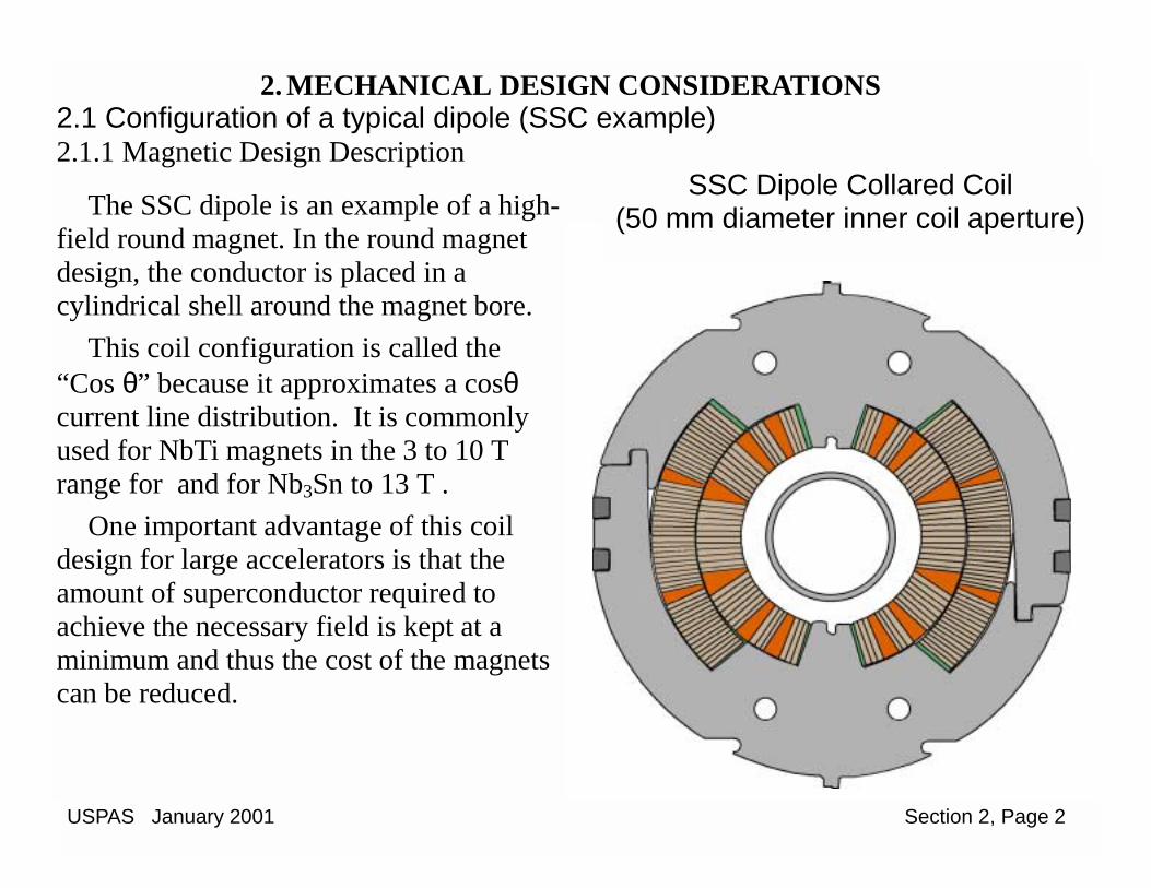
The SSC dipole is an example of a high-
field round magnet. In the round magnet design, the conductor is placed in a cylindrical shell around the magnet bore.
This coil configuration is called the “Cos θ” because it approximates a cosθ current line distribution. It is commonly used for NbTi magnets in the 3 to 10 T range for and for Nb3Sn to 13 T .
One important advantage of this coil design for large accelerators is that the amount of superconductor required to achieve the necessary field is kept at a minimum and thus the cost of the magnets can be reduced.
SSC Dipole Collared Coil (50 mm diameter inner coil aperture)

USPAS January 2001 Section 2, Page 3
The magnetic design calculations provide a table of the coordinates of each corner of every cable turn in the coil. These cable positions were calculated to produce the optimized field consistent with the tolerance on the allowed multipole components. The calculations were based on a cable size, which includes an insulation wrap and the effects of compression that occurs when the coil is assembled into the magnet.
2.1.1 Magnetic Design Description, continued

USPAS January 2001 Section 2, Page 4
After the magnetic design has been completed, the next step is to integrate it into the mechanical design of the magnet. The assembly of the coil, yoke and helium containment shell is called the cold mass. This is cooled with supercritical helium which flows axially through the flow channels and the space between the beam tube and the coils.
Channels are provided for the passage of the electrical bus for powering and interconnecting the magnets.
SSC Dipole Cold Mass Cross Section
2.1.2 Cold Mass: Integrating the Magnetic Design

USPAS January 2001 Section 2, Page 5
Since this magnet is a “cold iron” design, the entire cold mass assembly needs to be cooled to operating temperature. Thus, the cold mass is mounted in a cryostat which provides the necessary heat insulation and support system.
2.1.3. SSC Dipole Cryostat
4.5 K Liquid He Vacuum vessel
Cold mass
80 K Thermal shield
20 K Thermal shield
80 K Liquid N2
20 K He gas
Cold mass support

USPAS January 2001 Section 2, Page 6
This shows many of the detailed parts of the SSC dipole cryostat assembly as developed at FNAL.
2.1.3. SSC Dipole Cryostat, continued

USPAS January 2001 Section 2, Page 7
2.2 Mechanical Design Requirements
2.2.1 General Considerations
Superconducting accelerator magnets are high precision devices that must perform in very demanding situations. Special efforts are required to ensure that designs satisfy the following conditions:
1. The coils must be adequately supported to resist the very high Lorentz force loads. A well designed magnet is one which reaches the “short sample limit” of the conductor without quenching or excessive training.
2. The coils must be properly insulated to prevent electrical breakdown from the high voltages that can be induced during a quench.
3. The operating temperature of the coils must be kept within the required range for the specified superconductor.
4. Over its required lifetime, the magnet must not be degraded by exposure to the high radiation levels that would be present in an accelerator environment.
5. Materials used in the construction must retain adequate strength and ductility at operating temperature when subject to tensile stress.
USPAS January 2001 Section 2, Page 8
2.2.2 Lorentz force loads Minimum Quench Energy:
It has been estimated* that the minimum energy that will quench a NbTi cable operating at 90% of its critical current density (Jc) at 4.2 K and 6 T is of the order of a few µJ/mm3. This corresponds to the amount of work that would be done by the electromagnetic force applied to a strand of 0.8 mm diameter, carrying 100 A and moving by a few µm in a field of 6 T.
If the motions are purely elastic, no heat is dissipated and the coil remains superconducting. However, if the motions are frictional, the associated heat dissipation may be sufficient to cause a quench.
Thus, a coil support system that limits the motion of the conductor to a very small amount under the action of the Lorentz forces is a primary consideration in magnet design.
(Other factors affect the quenching of superconducting magnets such as ramp rate sensitivity and the Cu:SC of the conductor. The method of supporting the cable turns at the coil ends is also important. However, in this course we will limit our discussion primarily to the mechanical design of the 2-D cross section of the cold mass.)
2.2 Mechanical Design Requirements, continued
* For example, A. Devred, “Lectures on Accelerator Magnets”, 1992, 1994, 1999

USPAS January 2001 Section 2, Page 9
In the example given of the cosθ coil configuration for the SSC dipole, the magnetic design has produced a table of the coordinates of each of the conductor turns in the cross section of the coil. Thus, the Lorentz force vector acting at the centroid of each turn can be computed from the field and current for each turn or at the centroid of a block of turns.
By summing the results of the calculations for each block, the total X-direction and the Y-direction forces on each block of turns in a coil quadrant can be determined.
BLOCK FX, lb./in FY, lb/in FX,N/m FY,N/m 1 1005.46 -108.98 1.76E+05 -1.91E+04 2 1312.68 -237.56 2.30E+05 -4.16E+04 3 612.52 -151.97 1.07E+05 -2.66E+04 4 650.99 -116.62 1.14E+05 -2.04E+04 5 231.73 -384.60 4.06E+04 -6.74E+04 6 1208.86 -1371.22 2.12E+05 -2.40E+05
Total 5022.24 -2370.96 8.80E+05 -4.15E+05
2.2.2 Lorentz force loads, continued
The table summarizes the forces on the blocks in the example SSC dipole.

USPAS January 2001 Section 2, Page 10
These forces apply to the two dimensional cross section along the straight section of the coil. They are used to determine the structural response of the cold mass to the Lorentz force loading of the cross section.
The magnetic field also produces a longitudinal force that acts on the ends of the coil and tends to stretch it along its length. The magnitude of this force can be obtained from the Lorentz forces on the 2-D cross section of the coil and is independent of the arrangement of the end turns of the coil. [Example on next page]
SSC Dipole Coil End (Lead end shown)
The SSC dipole, operating at 6.6 T , produced an end force of 54 kN (12,000 lb) on the coil.
Thus, the ends of the magnet must be supported to resist this force and prevent axial motion which could induce quenches in the ends.
2.2.2 Lorentz force loads, continued
USPAS January 2001 Section 2, Page 11
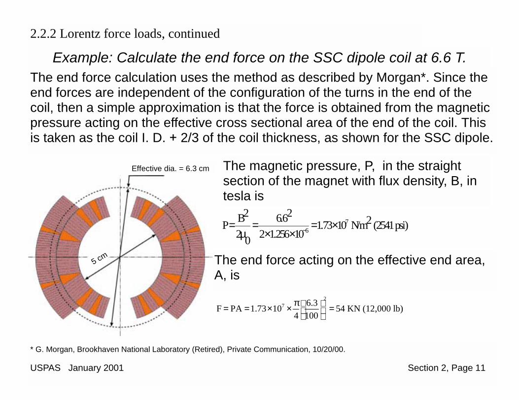
Example: Calculate the end force on the SSC dipole coil at 6.6 T. The end force calculation uses the method as described by Morgan*. Since the end forces are independent of the configuration of the turns in the end of the coil, then a simple approximation is that the force is obtained from the magnetic pressure acting on the effective cross sectional area of the end of the coil. This is taken as the coil I. D. + 2/3 of the coil thickness, as shown for the SSC dipole.
* G. Morgan, Brookhaven National Laboratory (Retired), Private Communication, 10/20/00.
Effective dia. = 6.3 cm
5 cm
The magnetic pressure, P, in the straight section of the magnet with flux density, B, in tesla is
76
2 2B 6.6 2P 1.73 10 N/m (2541 psi)2 2 1.256 100
−= = = ×µ × ×
The end force acting on the effective end area, A, is
27 6.3F PA 1.73 10 54 KN (12,000 lb)
4 100π = = × × =
2.2.2 Lorentz force loads, continued

USPAS January 2001 Section 2, Page 12
2.2.2 Lorentz force loads, continued
Coil Pre-stress requirements
In a cosθ coil there is a considerable azimuthal component of the Lorentz force acting on the circular arc. This will tend to compress the coil in the azimuthal direction and deflect it away from the pole. If such deflection is accompanied by a stick-slip type motion in the conductor cable, there could be sufficient energy deposited to initiate a quench*. The potential for coil motion at the pole can be eliminated by pre-loading the coils with sufficient azimuthal force that under operating conditions, the azimuthal Lorentz forces do not exceed the compressive pre-stress. This criterion has been routinely used as a requirement for pre-stress for coils in cosθ magnets.
If we were to specify the pre-stress requirements for a particular magnet assembly, we could use the SSC dipole as an example. In this case the azimuthal Lorentz force acting on the inner coil (Page 9) is -4.3 x 10⁵ N/m (-2450 lb/in) at 6.6 T. Since the width of the cable is 10 mm, then the compressive pre-stress to balance the Lorentz force would be 43 MPa (6300 psi). The compressive stress applied to the assembled coil at ambient temperature should be about 70 MPa (10,000 psi) to allow for loss of stress from cool down. *This effect has not been observed in actual magnet testing. In the SSC magnet development program no correlation was observed between coil pre-stress and quench performance. A special study done at BNL on an SSC model magnet did not find any observable effect on quench performance when the pre-stress level was reduced to a low level and the magnet was retested. Ref. P. Wanderer et al., “Effect of Prestress on Performance of a 1.8 m SSC R&D Dipole”, BNL report 45719, March 1991.

USPAS January 2001 Section 2, Page 13
Other configurations: A common coil design magnet [1] has been proposed for high field dipole
applications. The configuration of the coils are shown below:
1 Gupta, R., A Common Coil Design for High Field 2-in-1 Accelerator Magnets, Proceedings of the 1997 Particle Accelerator Conference.
Main coils for the 2-in-1 common coil design
2.2.2 Lorentz force loads, continued
USPAS January 2001 Section 2, Page 14
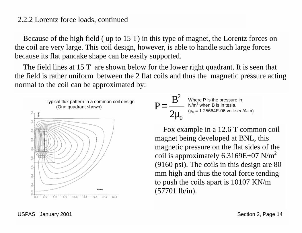
Because of the high field ( up to 15 T) in this type of magnet, the Lorentz forces on the coil are very large. This coil design, however, is able to handle such large forces because its flat pancake shape can be easily supported.
The field lines at 15 T are shown below for the lower right quadrant. It is seen that the field is rather uniform between the 2 flat coils and thus the magnetic pressure acting normal to the coil can be approximated by:
2
0
BP2
=µ
Where P is the pressure in N/m2 when B is in tesla. (µ0 = 1.25664E-06 volt-sec/A-m)
Typical flux pattern in a common coil design (One quadrant shown)
Fox example in a 12.6 T common coil magnet being developed at BNL, this magnetic pressure on the flat sides of the coil is approximately 6.3169E+07 N/m2 (9160 psi). The coils in this design are 80 mm high and thus the total force tending to push the coils apart is 10107 KN/m (57701 lb/in).
2.2.2 Lorentz force loads, continued

USPAS January 2001 Section 2, Page 15
Direction and an axial force, B, on the coil ends. At a nominal field of 12.6 T for 80 mm high coils and a 70 mm gap, these forces* are:
Total coil separation force
10,107 kN/m
57,700 lb/in
Axial end force on coil Xxxx kN** Xxxxx lb**
Net vertical compressive force on coil
-250 kN/m -1427 lb/in
80
70
*R. Gupta, Poisson calculation, 9/25/00 ** Calculate as an example.
2.2.2 Lorentz force loads, continued
The direction of the forces acting on this example common coil configuration are shown in the figure. In addition to the very large force, A, tending to push the coils apart, there is a net compressive force, C, tending to squeeze the coils in the vertical
A
B
C
C

USPAS January 2001 Section 2, Page 16
2.2.3 Steady state and transient thermal loads
Initial strain As a result of magnet assembly, certain of the components are in a state of initial
strain. In a typical assembly operation for a cosθ type dipole, the coils are pre-compressed
by enclosing them in interlocking collar packs (on top an bottom) in a collaring press. The collars are locked in position with keys.
The press platen comes down and squeezes the interleaving collars together.
Then the keys are inserted into the collar so that the coils are under an initial compressive stress.
The figure shows a collaring press used at FNAL for SSC dipoles.

USPAS January 2001 Section 2, Page 17
2.2.3 Steady state and transient thermal loads, continued
An additional initial strain is imparted to the assembly when the helium containment shell is welded around the collared coil and yoke. The shrinkage of the weld causes the shell to go into tension and therefore compresses the yoke-coil assembly. This action closes any gaps between the yoke halves and between the collared coil and yoke.
Initial strain in assembled cold mass
Helium containment shell in tension
Gaps have been closed
He shell weld has produced tension
Coils in compression
Collars still nominally in tension

USPAS January 2001 Section 2, Page 18
Thermal strain As the cold mass is cooled down to operating temperature (typically from ambient to
~ 4.5K), certain thermal strains are induced in the magnet materials due to the differences in the thermal contraction characteristics of the materials. Thermal strains can cause an increase or decrease in the stress in magnet components or even cause gaps to appear between them. The thermal strain is superimposed on the initial strain. The principal materials contributing to the thermal strain in the assembly are shown below.
Relative thermal strain (e/eFe ) of materials to yoke iron from 293 K to 4.2 K
304 SS 1.46 Yoke Iron 1.00 N40 collar 1.24 Alum collar 1.99 Hi Mn collar 0.80 Copper 1.61 Coil Az 3.06
Note: Properties of these common magnet construction materials will be discussed in the next section.
2.2.3 Steady state and transient thermal loads, continued

USPAS January 2001 Section 2, Page 19
Interpretation for steady state cool down effects: 1. Shell tensile stress increases. 2. Yoke stays firmly compressed. 3. Aluminum collars loosen away from yoke significantly. 4. Nitronic 40 collars loosen away from yoke slightly. 5. Hi Mn steel collars make tighter contact with the yoke. 6. Coil compressive pre-stress is reduced significantly with
Nitronic 40 or Hi Mn steel collars. 7. Coil compressive pre-stress is reduced slightly with
aluminum collars.
2.2.3 Steady state and transient thermal loads, continued
The significance of these effects will be treated in some detail in Section 4 on Approaches to Cold Mass Design.
304 SS 1.46 Yoke Iron 1.00 N40 collar 1.24 Alum collar 1.99 Hi Mn collar 0.80 Copper 1.61 Coil Az 3.06
e/eFe

USPAS January 2001 Section 2, Page 20
Transient thermal loads When magnets are mounted in a test facility or when they are connected in a string of
magnets, helium gas is used to cool the magnets to operating temperature. For the case of the SSC and RHIC, the gas flows at a rate of about 100 gram/sec through the magnet. Approximately 1 gm/sec of this flow is diverted to pass between the inner coil and the beam tube, as shown in this early version of an SSC dipole.
These helium flow passages carry about 99 gm/sec.
~ 1 gm/sec of helium flows between beam tube and coil.
Note that the beam tube is thermally isolated from the cold mass by means of insulated spacers.
2.2.3 Steady state and transient thermal loads, continued

USPAS January 2001 Section 2, Page 21
Even though only 1 % of the flow passes around the beam tube, its thermal mass is so low compared to that of the rest of the cold mass that it could cool down first. If it is assumed that this happens, then the beam tube would experience a maximum stress of :
6tE 28 10 .00284 ~ 80,000 psi (551 MPa)σ = ε = × × =
Where σ is the longitudinal tensile stress, E is the elastic modulus (psi) and εt is the thermal strain of stainless steel from 393 K to 4.2 K. Since this stress is above the yield point of the material, this situation needs to be taken into consideration in the mechanical design. A straight forward solution to this problem is to provide a bellows between the beam tube and its connection to the cold mass so that the beam tube is not rigidly contrained. This reduces the transient thermal stress to a very low value.
Beam tube
Portion of end of Cold mass
Beam tube welded to bellows
Bellows
Power lead
2.2.3 Steady state and transient thermal loads, continued

USPAS January 2001 Section 2, Page 22
2.2.4 Electrical stress and insulation requirements
High field dipole magnets, although rather small in aperture, are quite long. Thus, the magnetic volume is rather high and the energy content in the magnetic field is significant (Typical SSC dipole E=1.47 MJ). In a quenching situation, the energy in the magnet needs to be dissipated rapidly over a large volume of the coil or in an external resistance in order to limit the hot spot temperature in the coil (to prevent degradation or damage to the conductor or insulation).
Exploded view of an SSC dipole coil showing insulation strips and quench
protection heater.
Coil compression adjustment shim
Stainless steel quench protection heater strip, 0.004” thick.
Kapton insulation strips, typically 0.002” - 0.005” thick.
In accelerator magnets this is done by firing quench protection heaters mounted in the coil. This effectively increases the resistance of the discharging coil* and thus lowers the time constant so that the current decays rapidly. However, this produces a rather high voltage, typically 1 kV across the magnet coils and produces electrical stress on the coil insulation.
* This causes more of the coil to quench rapidly and thus increases the effective resistance. At the same time, more energy is deposited in a larger volume of the coil which produces less of a local temperature rise.

USPAS January 2001 Section 2, Page 23
The insulation requirements for the coil components are based on the Hipot test that is performed on the coil as a quality assurance check after the magnet is assembled.
It is customary for the Hipot test to apply a factor of safety of 4 or 5 to the expected peak voltage . Thus, the insulation rating to ground should be about 5 kV. Since the voltage is split between the two coil halves, that Hipot test is typically 3 kV.
Since the total voltage across the coil is distributed among the turns, the turn to turn insulation is tested at 70V. This requires a dynamic test rather than a static one to induce the voltage between the turns.
Note: The dielectric strength of Kapton film is about 5 kV/mil. However, redundant and thicker layers are used since the material could contain pin holes and is subject to damage under the high temperature and pressure in coil molding and high compressive stresses on the coil is collaring and assembly. Another factor to keep in mind is that the Hipot test is performed at atmospheric pressure where the dielectric strength of air is low and thus all un-insulated conductive surfaces exposed to 5 kV should be separated by at least 10 mm.
2.2.4 Electrical stress and insulation requirements, continued

USPAS January 2001 Section 2, Page 24
The cable turn positions in the magnetic design (as shown in Section 2.2.1) have been determined from magnetic analysis to optimize the (allowed) multipole content of the field. Conductor positioning tolerances for cosθ magnets are based on field quality requirements. A certain set of allowed multipoles content for the field is usually specified for the magnet and the accuracy of the position of the conductors has to be good enough to achieve this requirement.
2.2.5 Conductor positioning and tolerance requirements
For the design shown, the first 2 estimated systematic multipoles at 6.6 T are:
b2 = 0.51 units b4 = 0.03 units However, these calculated values are for
the ideal conductor position. In practice this is not attained and the multipoles will be different and related to the geometric tolerances that are used for the cold mass parts.

USPAS January 2001 Section 2, Page 25
In order to determine the effect of variations in conductor position on multipoles, we will reference a study made on variations of the position of the coil blocks, the thickness of the wedges and the variation in pole angle for the inner and outer coil. The results of such a study were reported by Gupta.*
* R. Gupta, IMPROVING THE DESIGN AND ANALYSIS OF SUPERCONDUCTING MAGNETS FOR PARTICLE ACCELERATORS, PhD. Thesis, Nov. 1996
4
2
3 6
5
1
1
2
3
4
This study (originally performed by P. A. Thompson ) imposed a change in block radial position of 0.05 mm (2 mils), a change in thickness of the wedges of 0.05 mm and a change in pole angle of typically 0.075°.
Each one of these variation produced changes in b2 of about 50% of the nominal value and in b4 of about 100% of the nominal value.
Thus, it follows that in order to obtain consistent field quality the parts that control the coil size and shape need to be toleranced at the level of about 0.025 mm (1 mil).
2.2.5 Conductor positioning and tolerance requirements, continued
USPAS January 2001 Section 2, Page 26
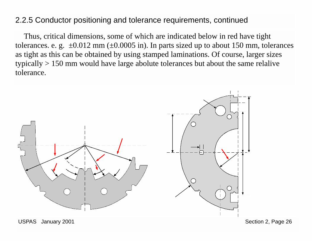
2.2.5 Conductor positioning and tolerance requirements, continued
Thus, critical dimensions, some of which are indicated below in red have tight tolerances. e. g. ±0.012 mm (±0.0005 in). In parts sized up to about 150 mm, tolerances as tight as this can be obtained by using stamped laminations. Of course, larger sizes typically > 150 mm would have large abolute tolerances but about the same relalive tolerance.

USPAS January 2001 Section 2, Page 27
2.2.6 Cold mass cooling requirements In addition to the heat that needs to be removed from the cold mass that arises from
the external environment at ambient temperature, other heat sources to consider are: 1. Synchrotron radiation 2. Energy deposition from charged particles (if the magnet is near a beam interaction
region) The special cooling requirements for magnets near high energy interactions regions are not considered here; however, we will use synchrotron radiation in the SSC dipole as an example.
In this diagram of an SSC dipole, He flow is indicated by the blue arrows and the nitrogen for the shield by a green arrow. About 99 g/sec of He flow through the bypass holes and 1 g/sec in the space between the coils and beam tube.
80K shield 20K shield
Bypass holes
Shield pipes
He return pipe

USPAS January 2001 Section 2, Page 28
2.2.6 Cold mass cooling requirements, continued
The type of cooling indicated by the heat flow path in the figure is called “diffusion cooling”. That is the interior parts of the cold mass including the coils, collars and yoke are cooled by a radial heat flow between the beam tube and the bypass holes.
Diffusion cooling is adequate to take care of the ambient heat load. For a 17 m long SSC dipole the ambient heat load is about 1 W. However since the magnet is long and the coils are covered with a low conductivity Kapton insulation, this type of cooling may not be adequate for the case of synchrotron radiation load which comes in through the beam tube.
In order to handle the heat flux from synchrotron radiation, which for the SSC dipole was estimated at 2 W per magnet at 20 TeV, an improved cooling scheme was required. This was done by directing the helium flow radially from the bypass holes to the beam rube area using a series of periodic baffles in the yoke. The scheme is called “cross flow cooling”*. * Shutt, R. and Rehak, M, “TRANSVERSE COOLING IN SSC MAGNETS”, Supercollider 2, Plenum Press, New York 1990.
Heat flow in diffusion cooling

USPAS January 2001 Section 2, Page 29
2.2.6 Cold mass cooling requirements, continued Principle of Cross Flow Cooling: The two upper bypass holes have restrictors at the
exit end and the two lower ones at the entrance end. This causes a pressure difference between the upper and lower holes so that the flow is forced through the channels into the collar packs and around the beam tube. The flow then travels axially and radially through the collar packs around the coil as diverted by baffles in the collar packs.
He bypass hole with restriction at exit end
25 x 1.5 mm channel opening every 30 cm
Collars have notches with a baffle in the center of each collar pack and pole openings. Radial flow occurs at collar pack ends.
Annular space around beam tube for He flow
Openings alternating with above, every 30 cm.
He bypass hole with restriction at entrance end

USPAS January 2001 Section 2, Page 30
29A
Cross Flow Cooling Diagram

USPAS January 2001 Section 2, Page 31
2.2.6 Cold mass cooling requirements, continued
Effect of Cross Flow Cooling: The specification for the SSC dipole coil temperature increase was, for a synchrotron
radiation load Sr: ∆T ≤ 0.05 K for Sr= 2 W . The table shows the effect of using cross flow cooling with a total flow of 100 g/sec
compared with diffusion cooling using a 1.3 mm gap between the beam tube and inner coil.
Sr ∆T , diffusion ∆T, cross flow
2 W 0.06 K 0.009 K
20 W n/a 0.044 K
Maximum temperature increase along coil (Computed)
USPAS January 2001 Section 2, Page 32
2.2.7 Other Loads The complete mechanical design procedure for an accelerator magnet requires
consideration of other loads, such as pressure, gravity and acceleration. In addition there is usually a radiation resistance requirements for the organic and composite materials used in accelerator magnet insulation and coil end parts.
Acceleration and gravity loads primarily effect the method for supporting the cold mass and influence the design and number of the cold mass supports. Pressure loads influence the design of the cryostat components such as the vacuum vessel and plumbing. For completeness, these loads are mentioned here; however a discussion of how they effect the design is not included.

USPAS January 2001 Section 2, Page 33
2.2.8 Cost Effective Design A high energy particle accelerator will contain many similar magnets. The number of
dipoles required in the arcs of some accelerators are listed below.
* 2 coils per yoke
Accelerator Number of Arc dipoles Tevatron 774
HERA 416 SSC 7964 RHIC 264 LHC 1792*
The mechanical design should take into account the necessity to minimize the cost of the magnets. This is particularly important since funding for accelerator projects unusually come from non-defense scientific budgets. Thus, cost reduction methods should be followed, some of which are indicated below:
1. Avoid the use of machined components. Use stacks of stamped laminations where possible to achieve high precision and low cost and precision molded plastic parts.
2. Use the lowest cost material that will satisfy performance requirements. 3. Avoid over-tolerancing of parts (this is sometimes difficult; however, it is a major
cost driver)

USPAS January, 2001 Section 3, Page 1
SUPERCONDUCTING ACCELERATOR MAGNETS
An Introduction to Mechanical Design and Construction Methods Carl L. Goodzeit ( BNL, ret.)
Note: Some of the material presented in this course was taken from: “Superconducting Accelerator Magnets”, an interactive CD ROM tutorial published by MJB Plus Inc.
(www.mjb-plus.com)
Section 3. Materials
© 2001 Carl L. Goodzeit All rights reserved.

USPAS January, 2001 Section 3, Page 2
1. INTRODUCTION 3.1. Introduction
This section describes some typical structural materials for superconducting magnets. It includes some data on the mechanical and physical properties of these materials that could be useful as reference information. It does not include a discussion of thermal and electrical properties, except for magnetic permeability, which is an important consideration for certain magnet parts.
The object of this section is to gain familiarity with a few grades of the materials used in magnet construction and some of the properties relevant to their use in superconducting magnet components. For example, there are many different grades of aluminum alloys and austenitic stainless steels. Previously distributed material recommended that the necessary background information about the various grades and designations for these materials be obtained prior to this presentation from the following sources:
Aluminum alloys: www.aluminum.org (Link to “Technology” and then “development of new applications for aluminum” then download “applications.pdf”.)
Stainless steel: www.ssinc.com (Link to “information for students”.) Also www.bssa.org.uk has some stainless steel background information that may be
useful.

USPAS January, 2001 Section 3, Page 3
3.1. Introduction, continued
Materials Table for Reference
Type of Material Typical Magnet Application Properties Listed
Aluminum alloys Collars, tubular products, various structural parts, welded parts
Mechanical Thermal contraction
Austenitic stainless steels Collars, structural parts, tubular products, plates and shells, welded parts
Mechanical Thermal contraction Magnetic permeability
Low carbon steel Magnet yokes Mechanical Thermal contraction Magnetic permeability
Other special steels N40, Hi-Mn, Invar
Collars, special parts Mechanical Thermal contraction Permeability
Copper and alloys Coil spacers, machined and stamped parts
Mechanical Thermal contraction
Composite Rutherford cable with insulation
Magnet coils Mechanical Thermal contraction
Plastics and composites Insulating pieces, coil end parts, shims
Mechanical Thermal contraction
USPAS January, 2001 Section 3, Page 4
3.2. Overview of Materials Characteristics
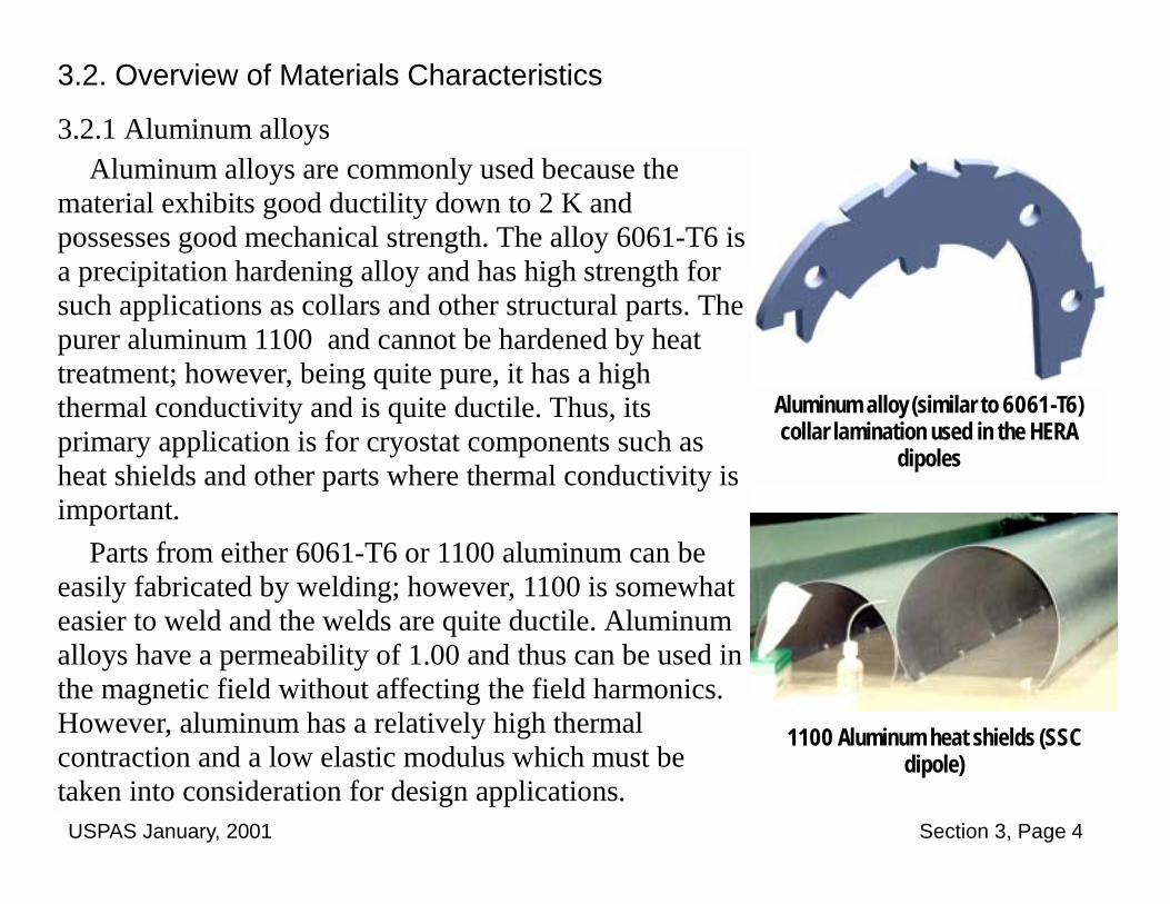
3.2.1 Aluminum alloys Aluminum alloys are commonly used because the
material exhibits good ductility down to 2 K and possesses good mechanical strength. The alloy 6061-T6 is a precipitation hardening alloy and has high strength for such applications as collars and other structural parts. The purer aluminum 1100 and cannot be hardened by heat treatment; however, being quite pure, it has a high thermal conductivity and is quite ductile. Thus, its primary application is for cryostat components such as heat shields and other parts where thermal conductivity is important.
Parts from either 6061-T6 or 1100 aluminum can be easily fabricated by welding; however, 1100 is somewhat easier to weld and the welds are quite ductile. Aluminum alloys have a permeability of 1.00 and thus can be used in the magnetic field without affecting the field harmonics. However, aluminum has a relatively high thermal contraction and a low elastic modulus which must be taken into consideration for design applications.
Aluminum alloy (similar to 6061-T6) collar lamination used in the HERA
dipoles
1100 Aluminum heat shields (SSC dipole)

USPAS January, 2001 Section 3, Page 5
As seen in the ‘tree’ diagram on the website for the Stainless Steel Institute of North America (www.ssina.com), the Fe, Cr, Ni system produces a complicated series of alloys. The term “stainless steel” (without any qualifiers) always refers to the austenitic type of stainless steel (300 series). This structure is characterized by having a face centered cubic (FCC) crystal lattice, which has the properties of being ductile down to 2 K and having permeability near 1.00 (depending on grade).
3.2.2. Austenitic stainless steels
The 300 series alloys cannot be hardened by heat treatment. However, cold work (such as rolling into sheets or drawing into wire) can significantly enhance the tensile strength and also increase the permeability. Most stainless steel products are supplied in the annealed condition, which cancels the strengthening and permeability effects from the cold work. However, the strength of stainless steel is adequate for most superconducting magnet applications.
Stainless steel is readily welded and produces strong, ductile welds so that it is useful for such important applications as pressure vessels, beam tubes, collars and essentially all helium containment vessel parts.
Collar pack (Nitronic 40 stainless steel) from an SSC prototype dipole
USPAS January, 2001 Section 3, Page 6
3.2.2. Austenitic stainless steels, continued
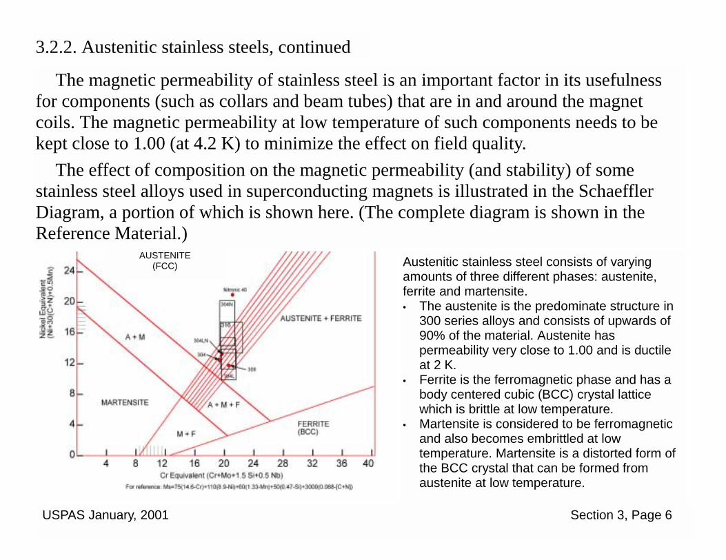
The magnetic permeability of stainless steel is an important factor in its usefulness for components (such as collars and beam tubes) that are in and around the magnet coils. The magnetic permeability at low temperature of such components needs to be kept close to 1.00 (at 4.2 K) to minimize the effect on field quality.
The effect of composition on the magnetic permeability (and stability) of some stainless steel alloys used in superconducting magnets is illustrated in the Schaeffler Diagram, a portion of which is shown here. (The complete diagram is shown in the Reference Material.)
Austenitic stainless steel consists of varying amounts of three different phases: austenite, ferrite and martensite. • The austenite is the predominate structure in
300 series alloys and consists of upwards of 90% of the material. Austenite has permeability very close to 1.00 and is ductile at 2 K.
• Ferrite is the ferromagnetic phase and has a body centered cubic (BCC) crystal lattice which is brittle at low temperature.
• Martensite is considered to be ferromagnetic and also becomes embrittled at low temperature. Martensite is a distorted form of the BCC crystal that can be formed from austenite at low temperature.
AUSTENITE (FCC)

USPAS January, 2001 Section 3, Page 7
3.2.2. Austenitic stainless steels, continued The ratio of the amount of austenite to martensite can be controlled by the Cr-Ni
balance in the material as shown in the Shaeffler Diagram. Higher Cr produces more ferrite while higher nickel produces more austenite. Certain elements act the same as Cr in forming ferrite and thus are used to adjust the “Cr equivalent”. Similarly other elements are austenite forming and are added to the “Ni equivalent”. Expressed in terms of the weight % in the alloy, these are: Cr Equivalent =Cr+Mo+1.5 Si+0.5 Nb Ni Equivalent = (Ni+30(C+N)+0.5Mn)
[Note the powerful austenizing effect of C and N] Another effect that occurs in stainless steel that depends on the ferrite content is
“spontaneous martensite transformation”. Below a specific transformation temperature, Ms, that is composition dependent, an irreversible transformation from austenite (non-magnetic, ductile) to martensite (magnetic, brittle at low temperature) can sometimes occur spontaneously. Ms=75(14.6-Cr)+110(8.9-Ni)+60(1.33-Mn)+50(0.47-Si)+3000(0.068-[C+N])
USPAS January, 2001 Section 3, Page 8
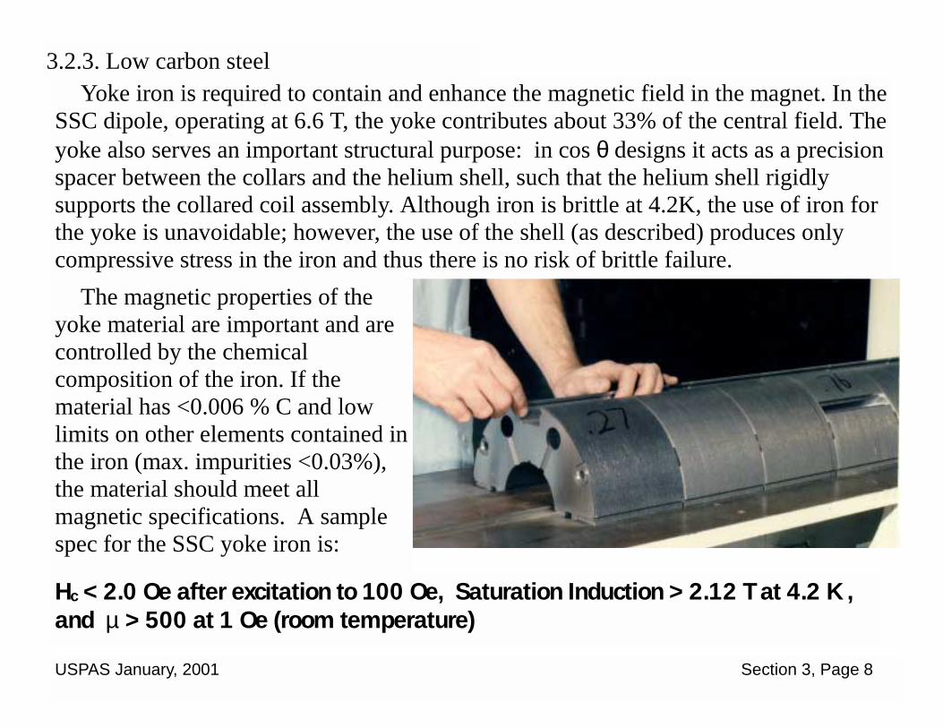
3.2.3. Low carbon steel Yoke iron is required to contain and enhance the magnetic field in the magnet. In the
SSC dipole, operating at 6.6 T, the yoke contributes about 33% of the central field. The yoke also serves an important structural purpose: in cos θ designs it acts as a precision spacer between the collars and the helium shell, such that the helium shell rigidly supports the collared coil assembly. Although iron is brittle at 4.2K, the use of iron for the yoke is unavoidable; however, the use of the shell (as described) produces only compressive stress in the iron and thus there is no risk of brittle failure.
The magnetic properties of the yoke material are important and are controlled by the chemical composition of the iron. If the material has <0.006 % C and low limits on other elements contained in the iron (max. impurities <0.03%), the material should meet all magnetic specifications. A sample spec for the SSC yoke iron is:
Hc < 2.0 Oe after excitation to 100 Oe, Saturation Induction > 2.12 T at 4.2 K , and µ > 500 at 1 Oe (room temperature)
USPAS January, 2001 Section 3, Page 9
3.2.4. Other special steels: Nitronic 40, Hi-Mn, Invar
Because of the special requirements for collars (i.e. high strength, low magnetic permeability) more common grades of stainless steel (304, 316) may not be appropriate. For a high field dipole design, it is desirable to keep the iron reasonably close to the coils (to minimize the size of the cold mass). Thus, a radial space of 10 mm between the coil O.D. and the yoke I.D. may be appropriate. The collar must fit into this space and be designed in such a way that the high pre-stress applied to the coils in the collaring operation does not overstress the material.
Two very useful collar materials were investigated in the SSC magnet development program: Nitronic 40* and Hi-Mn steel**. Both are high strength austenitic stainless steel materials and are indicated on the Schaeffler diagram as being 100% austenite. The high strength of these materials is obtained by cold work (i.e. cold rolling) which, because of the high stability of the austenite, does not produce martensite, and thus the material retains its low permeability.
The Hi-Mn steel has an interesting property in that its thermal contraction is actually less than that of the yoke iron; the implication of this is discussed in Section 6. However, recent inquiries have revealed that this material may be difficult to obtain currently because of environmental restrictions on the smelting of Mn.
*C: 0.025%, Mn: 9.00%, Cr: 21.00%, N:0.25%, Fe: Bal. ** C: 0.10 %, Mn: 28%, Ni: 1.00%, Cr: 7.10%, N: 0.1%, Fe: Bal.

USPAS January, 2001 Section 3, Page 10
3.2.4. Other special steels: Nitronic 40, Hi-Mn, Invar (continued)
Invar is another interesting material that may have some application in superconducting magnet design, particularly in cryogenic equipment (helium transfer lines). Invar is an iron alloy containing 36 % Ni. It has a very low thermal contraction (~0.044 % to 4.2K) and remains ductile at that temperature. However, the Curie temperature (below which ferromagnetism appears) is 276 C so the material is magnetic at low temperature. Nevertheless, it can be used for structural applications where it is advantageous to have a very low amount of thermal contraction.

USPAS January, 2001 Section 3, Page 11
Copper and its principal alloys (brasses, bronze) are all ductile at 4.2 K and can be used for structural components in superconducting magnets. Pure copper (OFHC) is used as wedges or spacers that are molded into the coils. The high thermal conductivity of this material is desirable for this application. Copper and its alloys possess a thermal contraction close to that of stainless steel so that they can be used in conjunction with stainless steel components without inducing significant thermal strain. Brass or bronze parts have been used as coil end spacers in magnets wound with Nb3Sn conductor. Composite plastic materials cannot be used for this application since the coil assembly is subject to high temperature (~800 C) during the heat treatment to form the Nb3Sn.
3.2.5. Copper and alloys
Machined cross section of a prototype SSC insertion region quadrupole showing copper and alloy parts.
Bronze keys
Brass spacers
Cu wedges
SS collar

USPAS January, 2001 Section 3, Page 12
3.2.6. Composite Rutherford cable with insulation
Currently, the standard conductor configuration (NbTi and even Nb3Sn) is a Rutherford type cable that is wrapped with insulation. For NbTi magnets, the insulation is coated with a thermosetting adhesive so that the coil can be molded at temperature and pressure to form a composite structure that can be handled and assembled into collars. Sometimes, rather than insulation with adhesive, an epoxy impregnated fiberglass layer is applied to the insulated cable and used to mold the coil into a stable shape.
The mechanical properties of the composite coil are an important consideration in the mechanics of the collaring and pre-stress application to the coil, as well as what happens when the magnet is cooled to operating temperature. In order to determine the compressive stress in the coil after assembly into the magnet and after cool down, it is necessary to know the stress-strain characteristics of the composite material as well as its thermal contraction properties. Since the coil composite is composed of a layer structure, its mechanical properties are orthotropic. Thus, the elastic modulus and thermal contraction are different in the longitudinal and azimuthal directions.
Fixture for measuring compressive modulus of cable
USPAS January, 2001 Section 3, Page 13
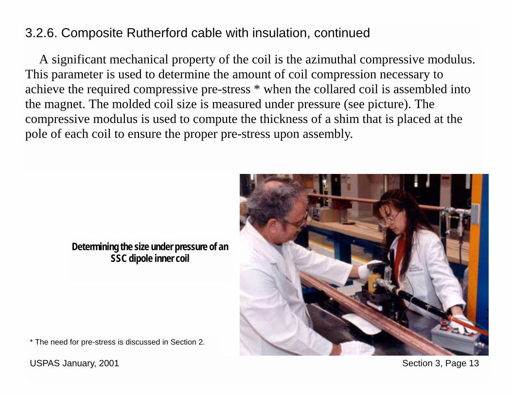
3.2.6. Composite Rutherford cable with insulation, continued
A significant mechanical property of the coil is the azimuthal compressive modulus. This parameter is used to determine the amount of coil compression necessary to achieve the required compressive pre-stress * when the collared coil is assembled into the magnet. The molded coil size is measured under pressure (see picture). The compressive modulus is used to compute the thickness of a shim that is placed at the pole of each coil to ensure the proper pre-stress upon assembly.
Determining the size under pressure of an SSC dipole inner coil
* The need for pre-stress is discussed in Section 2.

USPAS January, 2001 Section 3, Page 14
3.2.6. Composite Rutherford cable with insulation, continued
It is seen that the compressive modulus is related to the coil configuration. The curves for the inner and outer coils for the SSC dipole show that the inner coil has a higher compressive modulus than the outer. Also, the stress-strain curve is not linear. The compressive moduli at high and low strain values are shown in the table.
Compressive strain
Inner coil compressive modulus, MPa
Outer coil compressive modulus, MPa
-0.0002 5.3 3.6 -0.005 15.8 14.2
Coil stress vs. strain
0
10
20
30
40
50
60
70
80
0 0.002 0.004 0.006 0.008Compressive strain
Stre
ss, M
Pa
Inner CoilOuter Coil

USPAS January, 2001 Section 3, Page 15
3.2.7. Plastics and composites
Some critical components in a superconducting magnet are required to be structural electrical insulators or thermal insulators. Examples are supports for the conductor and bus work, spacers for the end turns of the coil, coil to ground insulation, and cold mass support posts (thermal load).
We also include in this category Kapton (a polyimide film) used for cable, coil and electrical bus insulation. Kapton is only produced in a film, which can be obtained typically in thickness up to 0.125 mm. Thus, its bulk mechanical properties are not relevant for structural applications.
SSC Dipole Coil End Parts (G10)
RHIC Support Post Component Ultem 2100
Kapton Insulation on SSC Coil

USPAS January, 2001 Section 3, Page 16
3.2.7. Plastics and composites, continued
Specific materials that have been used for structural applications are NEMA Grade G-10 (Fiberglass-epoxy laminate) and proprietary materials with trade names such as:
Spaulrad (Spaulding Composites, www.spauldingcom.com) RX630 (Rogers Corporation, www.rogers-corp.com) Ultem 2100 (GE Structured Products, www.structuredproducts.ge.com) In addition, commercial plastics such as Teflon and Nylon have been used for
superconducting magnet parts.
The proprietary composite materials indicated above have been used for magnet parts that were produced by injection molding. This process uses a precision die in which the material is molded under heat and pressure to produce the part. (Example: RHIC insulation spacer.) This process is ideal to keep the cost low when a large number of identical parts are required (i.e. >1000). For prototype magnet parts, however, individual pieces are machined and thus the unit cost is much higher.

USPAS January, 2001 Section 3, Page 17
3.2.7. Plastics and composites, continued
Radiation Resistance An important consideration for the choice of plastics and/or composite materials in
superconducting magnet applications is radiation resistance. If the superconducting magnet application involves exposure to high levels of radiation, then there may be a concern that these organic materials may suffer radiation damage and thus become degraded*. Note: Kapton film, which is used as the primary insulation for the coil in an area that could be subjected to the highest radiation intensity, is among the most resistant materials. It has been subjected to exposures of 109 rads at 4 K with little degradation. Kapton also has one of the highest temperature resistance ratings for any plastic material (i.e. can be used up to 400 C), which again is a desirable property since portions of the coil can become quite hot in the event of a quench.
The reference material, which has been previously distributed, contains mechanical property data, thermal contraction measurements and radiation resistance data** for most of these materials.
* The design dose for the radiation resistance of SSC magnet components was as follows: Materials in the cold mass, such as end parts, insulation, adhesives : 109 rads Materials outside the cold mass, such as support posts, electrical bus insulation and support parts: 108 rads ** From “Report on the Program of 4 K Irradiation of Insulating Materials for the Superconducting Super Collider”, by A. Spindel, July 8, 1993

USPAS January, 2001 Section 4, Page 1
SUPERCONDUCTING ACCELERATOR MAGNETS
An Introduction to Mechanical Design and Construction Methods Carl L. Goodzeit ( BNL, ret.)
Note: Some of the material presented in this course was taken from: “Superconducting Accelerator Magnets”, an interactive CD ROM tutorial published by MJB Plus Inc.
(www.mjb-plus.com)
Section 4. Approaches to Cold Mass Design: Magnet Types
© 2001 Carl L. Goodzeit All rights reserved.

USPAS January, 2001 Section 4, Page 2
4.1 Introduction
Various types of magnet design can be considered for accelerator applications. The principal parameter that governs the magnet type is the design field, which is based on the energy of the accelerated beam. Figure 1 shows the field for which various design types are applicable. (Note: There may be some overlap in these ranges).
We have already become familiar with the construction features of the SSC dipole. Thus, in this section we will look at examples of some other magnets in various field ranges that have been used for accelerators and consider how the designs were developed to meet the requirements.
USPAS January, 2001 Section 4, Page 3
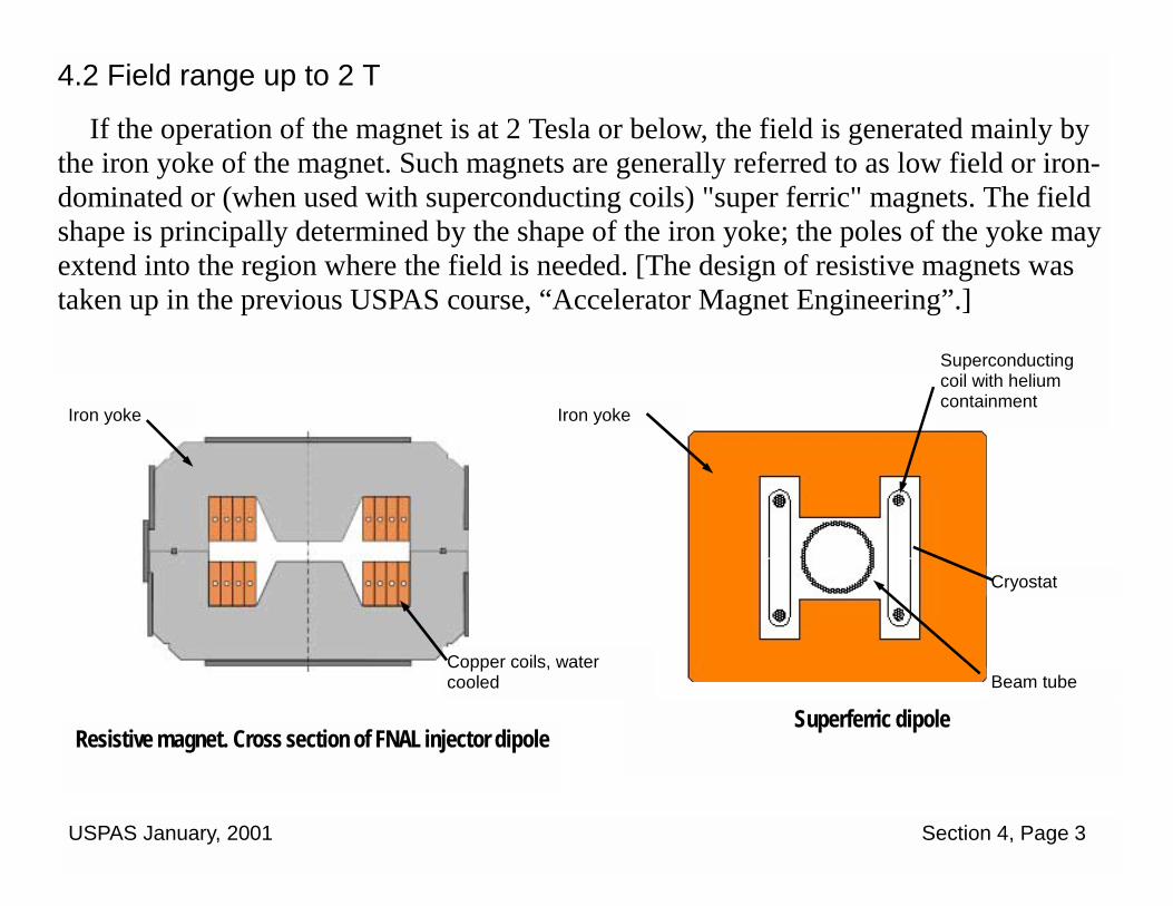
4.2 Field range up to 2 T
If the operation of the magnet is at 2 Tesla or below, the field is generated mainly by the iron yoke of the magnet. Such magnets are generally referred to as low field or iron-dominated or (when used with superconducting coils) "super ferric" magnets. The field shape is principally determined by the shape of the iron yoke; the poles of the yoke may extend into the region where the field is needed. [The design of resistive magnets was taken up in the previous USPAS course, “Accelerator Magnet Engineering”.]
Resistive magnet. Cross section of FNAL injector dipole Superferric dipole
Iron yoke
Superconducting coil with helium containment
Cryostat
Beam tube
Iron yoke
Copper coils, water cooled
USPAS January, 2001 Section 4, Page 4
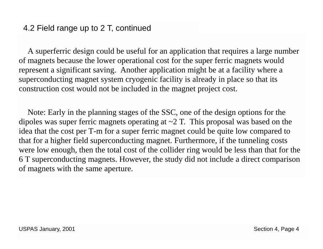
A superferric design could be useful for an application that requires a large number
of magnets because the lower operational cost for the super ferric magnets would represent a significant saving. Another application might be at a facility where a superconducting magnet system cryogenic facility is already in place so that its construction cost would not be included in the magnet project cost.
Note: Early in the planning stages of the SSC, one of the design options for the
dipoles was super ferric magnets operating at ~2 T. This proposal was based on the idea that the cost per T-m for a super ferric magnet could be quite low compared to that for a higher field superconducting magnet. Furthermore, if the tunneling costs were low enough, then the total cost of the collider ring would be less than that for the 6 T superconducting magnets. However, the study did not include a direct comparison of magnets with the same aperture.
4.2 Field range up to 2 T, continued

USPAS January, 2001 Section 4, Page 5
4.3 Field range 2 to 4.5 T
An efficient design to use in this field range is the single layer cosθ magnet design such as used for RHIC. Although this magnet was designed for an operating field of 3.4 T, it has been successfully operated at higher fields (However the magnetic design is not optimized for the higher field range). The specifications and components of this magnet are described in some detail in Lesson 1.7 of the CD-ROM Tutorial.
Stainless steel collaring key

USPAS January, 2001 Section 4, Page 6
Cold mass design approach: A single layer coil of NbTi at 4.3 K in an iron yoke can be designed to work in this range, without the need for separate collars to provide pre-stress.
A single layer coil requires only about half of the force to apply pre-stress to the coil as a two-layer coil. If we apply the criterion for pre-stress (Section 2.2.2), to balance the azimuthal Lorentz force at operating conditions by applying 40 MPa* of compressive stress to the coils, the maximum stress in any part of the yoke would not exceed the yield point of low carbon steel / iron. The successful RHIC design has shown that the yoke can perform the function of the collars.
Pair of RHIC yoke laminations pinned together to act as a collar
Question: Why is it necessary to use two laminations pinned
together for a collar rather than just single laminations?
Shear pin
4.3 Field range 2 to 4.5 T, continued
Derived from 26 MPa azimuthal Lorentz force pressure with a 33% pre-stress loss on cool down.

USPAS January, 2001 Section 4, Page 7
Although collars, per se, are not required in this design, we still require the coils to be held firmly in the proper geometry, with enough space between the coil and the iron to satisfy the magnetic design requirements. This has been accomplished in an efficient way by using injection molded pole spacers made of RX630; these also serve as insulators and thus eliminate the need for expensive Kapton coil insulation pieces.
The replacement of the expensive stainless steel collars with a mass-produced plastic part and the dual function of the yoke has resulted in an economical, “value engineered” design for this magnet.
This same method of cold mass construction has been applied to the RHIC quadrupoles and corrector magnets as well.
4.3 Field range 2 to 4.5 T, continued
RX 630 insulator/spacers placed around RHIC dipole coil.

USPAS January, 2001 Section 4, Page 8
4.4 Field range 4.5 to 7.5 T This is the range in which the 2-layer cosθ design using NbTi Rutherford type cable at
4.3 K has been proven to be the desired option. We have previously described the SSC dipole. The Tevatron dipole (on the left) was the first superconducting accelerator magnet that was designed, tested, and installed in an operating accelerator. The HERA dipole (on the right) is another example of a superconducting magnet that is currently operating. Specifications and construction details for these magnets can be found in Lesson 1.7 of the CD-ROM Tutorial.
Tevatron dipole. This magnet has a warm iron yoke and a collared coil assembly in a close-fitting cryostat. HERA dipole in cryostat

USPAS January, 2001 Section 4, Page 9
Tevatron dipole design approach: Yoke of warm iron is used, in order to minimize the time required to warm up and cool down the magnet string and thus maximize the accelerator up time. Hence, the cryostat for this magnet consists mainly of the collared coil, helium containment, and liquid nitrogen shield. This cryostat assembly is supported in the yoke by the method shown on the previous page.
This was the first magnet design that used collars to provide the coils with compressive pre-stress. The use of collars for cosθ magnet assemblies has been carried through to later magnets.
4.4 Field range 4.5 to 7.5 T, continued A
C
B
D
The cold mass is assembled in a compact cryostat which contains a liquid helium cooled shield and a liquid nitrogen cooled shield. A-Single phase (supercritical) helium B-Beam tube C-Liquid nitrogen shield D-Liquid helium shield (two-phase)
USPAS January, 2001 Section 4, Page 10
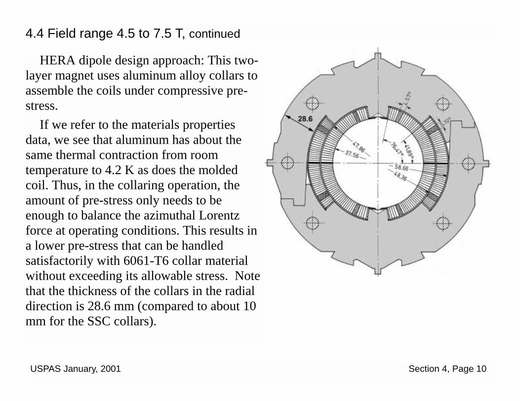
HERA dipole design approach: This two-layer magnet uses aluminum alloy collars to assemble the coils under compressive pre-stress.
If we refer to the materials properties data, we see that aluminum has about the same thermal contraction from room temperature to 4.2 K as does the molded coil. Thus, in the collaring operation, the amount of pre-stress only needs to be enough to balance the azimuthal Lorentz force at operating conditions. This results in a lower pre-stress that can be handled satisfactorily with 6061-T6 collar material without exceeding its allowable stress. Note that the thickness of the collars in the radial direction is 28.6 mm (compared to about 10 mm for the SSC collars).
4.4 Field range 4.5 to 7.5 T, continued

USPAS January, 2001 Section 4, Page 11
The HERA collars were designed to be “self supporting”, i.e., the radial deflection of the collared coil due to the horizontal component of the Lorentz force would be less than ~0.06 mm .
Thus, the collars do not require the yoke and shell as structural supports and are therefore mounted in the yoke with a slight amount of clearance. Indeed, this clearance increases as the magnet cools down since the thermal contraction of the collared coils is greater than that of the yoke.
4.4 Field range 4.5 to 7.5 T, continued
A
B
A - Nominal fit of HERA collar in yoke. B - Calculated deflection (dotted lines) of pre-stressed coils in collar. Room temperature coil is on the left and operating condition coil with Lorentz force is on the right. From K.-H. Mess, P. Schmuser and S. Wolff, “Superconducting Accelerator Magnets”, World Scientific Publishing Co. , Singapore

USPAS January, 2001 Section 4, Page 12
4.5 Field range 7.5 to 10 T NbTi cable magnets can attain this field
range provided that the operating temperature is that of super fluid helium at 1.9 K. Also, magnets can attain 10 T by using Nb3Sn at 4.3 K. However, the main application for Nb3Sn is in the higher field ranges where NbTi is unsatisfactory. (I assume that the conductor usage limits have been explained in the previous lectures.)
The LHC dipole magnet is designed for use in this range. This magnet is an example of a 2 in 1 cold mass that contains two dipole coils of opposite polarity in the common yoke. The history and current specifications for the magnet can be found from CERN’s website: www.cern.ch. Go to “LHC Project” and follow the links to “Magnets for the Ring” – “Main Dipole” – “MB”.
LHC Dipole Cross Section. This is an earlier version with a 50 mm inner coil aperture. The current aperture is 56 mm.

USPAS January, 2001 Section 4, Page 13
4.5 Field range 7.5 to 10 T, continued LHC dipole design approach: In order to achieve acceleration energy of 7 TeV in the
existing LEP tunnel, the dipoles most produce a field of about 9 T. Thus, it was decided to use NbTi at 1.9 K rather than Nb3Sn (although some early model magnets were made with this material). The side by side arrangement of the two apertures in the common yoke is a space saving feature that was required to permit installation of the LHC in the existing LEP tunnel with the LEP still intact. Thus a compact, high efficiency design is required. The design uses aluminum alloy collars and a vertically split yoke with a slight gap. On cool-down, the shrinkage of the outer helium containment shell will compress the yoke and close the gap in order to make the yoke conform to the collars and thus provide horizontal stiffness. (A description of a slightly earlier, but similar, design can be found in the CD-ROM tutorial Lesson 1.7. )
LHC dipole collar pack showing two types of laminations pinned together with shear pins.

USPAS January, 2001 Section 4, Page 14
4.6 Field Range 10 to 13 T For this field range, Nb3Sn at 4.3 K is the
principal conductor used in magnets. The D20 dipole magnet constructed at LBNL* is an example of the technique for working with Nb3Sn. The maximum field for this magnet is 13 T and it is obtained by using a 4-layer coil as shown. *D. Dell’Orco, R. Scanlan and C. Taylor, “Design of the Nb3Sn Dipole, D20”, LBL Report 32072 (not dated)
D20 Coil Cross Section
A B
C
D
D20 cross section A- Stainless steel shell (25 mm thick on 381 mm radius yoke) B- Aluminum spacer (280 mm wide) C- Tapered gap (0.56 -0.76 mm) D– Stainless steel collars (9 mm wide)
[Review properties of Nb3Sn conductor in Lesson 2.4]
USPAS January, 2001 Section 4, Page 15
4.6 Field Range 10 to 13 T, continued
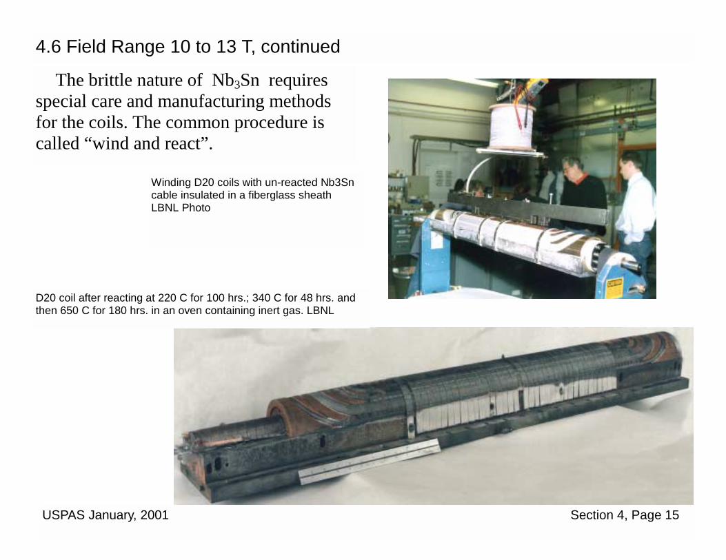
The brittle nature of Nb3Sn requires special care and manufacturing methods for the coils. The common procedure is called “wind and react”.
Winding D20 coils with un-reacted Nb3Sn cable insulated in a fiberglass sheath LBNL Photo
D20 coil after reacting at 220 C for 100 hrs.; 340 C for 48 hrs. and then 650 C for 180 hrs. in an oven containing inert gas. LBNL
USPAS January, 2001 Section 4, Page 16
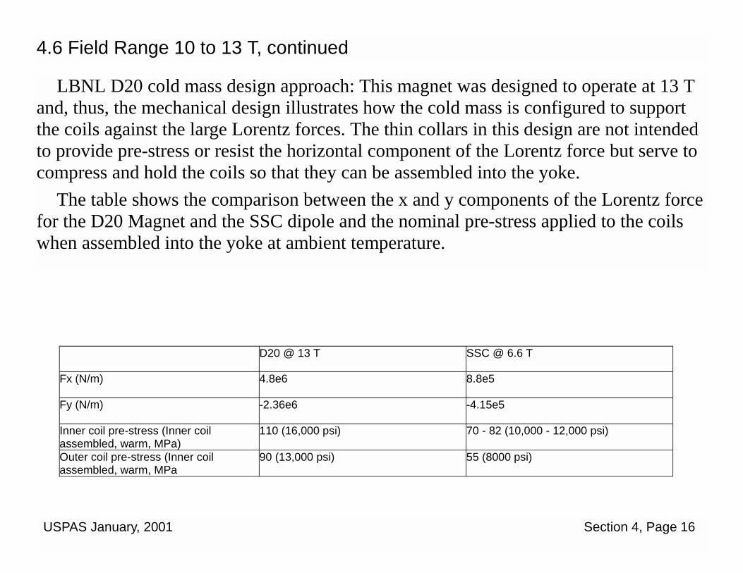
LBNL D20 cold mass design approach: This magnet was designed to operate at 13 T and, thus, the mechanical design illustrates how the cold mass is configured to support the coils against the large Lorentz forces. The thin collars in this design are not intended to provide pre-stress or resist the horizontal component of the Lorentz force but serve to compress and hold the coils so that they can be assembled into the yoke.
The table shows the comparison between the x and y components of the Lorentz force for the D20 Magnet and the SSC dipole and the nominal pre-stress applied to the coils when assembled into the yoke at ambient temperature.
4.6 Field Range 10 to 13 T, continued
D20 @ 13 T SSC @ 6.6 T
Fx (N/m) 4.8e6 8.8e5
Fy (N/m) -2.36e6 -4.15e5
Inner coil pre-stress (Inner coil assembled, warm, MPa)
110 (16,000 psi) 70 - 82 (10,000 - 12,000 psi)
Outer coil pre-stress (Inner coil assembled, warm, MPa
90 (13,000 psi) 55 (8000 psi)

USPAS January, 2001 Section 4, Page 17
4.6 Field Range 10 to 13 T, continued
However, the critical current for Nb3Sn conductor is sensitive to applied compressive stress. Thus there is a limit to the amount of pre-stress that should be applied to the coils.
The University of Twente made a study of this effect on several Nb3Sn cables, with the result seen in the figure. Note that the applied pre-stress level for this magnet could cause Ic degradation, depending on the conductor configuration.
We will see next that, for higher field magnets, a different design approach is used.
Data source: University of Twente
USPAS January, 2001 Section 4, Page 18
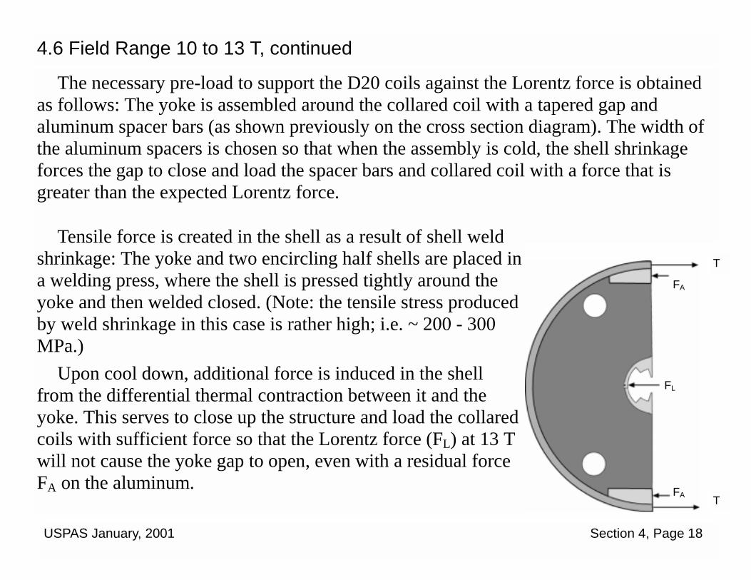
The necessary pre-load to support the D20 coils against the Lorentz force is obtained as follows: The yoke is assembled around the collared coil with a tapered gap and aluminum spacer bars (as shown previously on the cross section diagram). The width of the aluminum spacers is chosen so that when the assembly is cold, the shell shrinkage forces the gap to close and load the spacer bars and collared coil with a force that is greater than the expected Lorentz force.
4.6 Field Range 10 to 13 T, continued
Tensile force is created in the shell as a result of shell weld shrinkage: The yoke and two encircling half shells are placed in a welding press, where the shell is pressed tightly around the yoke and then welded closed. (Note: the tensile stress produced by weld shrinkage in this case is rather high; i.e. ~ 200 - 300 MPa.)
Upon cool down, additional force is induced in the shell from the differential thermal contraction between it and the yoke. This serves to close up the structure and load the collared coils with sufficient force so that the Lorentz force (FL) at 13 T will not cause the yoke gap to open, even with a residual force FA on the aluminum.
T
FA
FL
FA T
USPAS January, 2001 Section 4, Page 19
4.7 Field Range 13 to 16 T
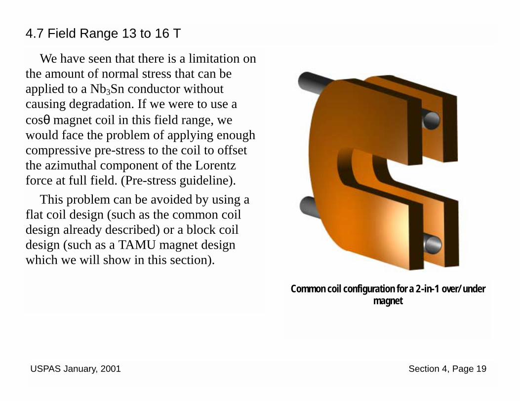
We have seen that there is a limitation on the amount of normal stress that can be applied to a Nb3Sn conductor without causing degradation. If we were to use a cosθ magnet coil in this field range, we would face the problem of applying enough compressive pre-stress to the coil to offset the azimuthal component of the Lorentz force at full field. (Pre-stress guideline).
This problem can be avoided by using a flat coil design (such as the common coil design already described) or a block coil design (such as a TAMU magnet design which we will show in this section).
Common coil configuration for a 2-in-1 over/under magnet

USPAS January, 2001 Section 4, Page 20
In Section 2.3.2 we saw that the horizontal Lorentz force acting on a flat coil (common coil design) was 10,107 kN/m at 12.6 T. This corresponds to a normal pressure (with a coil height of 80 mm) of 63 MPa between the coil and its support.
At 16 T this pressure rises to 101 MPa. [The epoxy impregnated coil composite is expected to withstand this pressure at 4.2 K.] The corresponding net vertical compressive pressure acting on the coil is 16 MPa; a vertical compressive force can be easily applied to compensate for this. However, the large horizontal Lorentz force needs to be transmitted to a coil support system that is rigid enough to prevent coil deflections that could cause training or premature quenching.
4.7 Field Range 13 to 16 T, continued
Directions of forces on common coils.

USPAS January, 2001 Section 4, Page 21
We will consider two approaches to methods of coil support at fields ~16 T. One example is a modification of the common coil design proposed by Gupta that is being developed at LBNL (1); the second is a ~15 T block coil dipole being developed at TAMU (2). These magnets are presently in the R&D phase and thus the designs have not yet been proven or finalized at the highest field levels. We will also limit our discussion to the two-dimensional cross section of the cold mass and not consider how the ends of the coil are supported. However, in any complete magnet design discussion this issue needs to be covered.
4.7 Field Range 13 to 16 T, continued
The first example is a common coil magnet assembly (~ 1 m long) called RD3 that was built at LBNL.
Primary concerns with magnets in the 16 T field range are: a. How to design the coils so that they are not overstressed or subject to significant
deflection under operating conditions. b. How to support the coils against the horizontal force without causing significant
coil deflections (i.e. <0.08 mm). (1) S. Caspi, et al., “RD3 Structure”, LBNL SC-Mag 712, June 15, 2000 S. Caspi, et al., “The Use of Pressurized Bladders for Stress Control of Superconducting Magnets”, Presented at ASC2000. (2) * P. McIntyre, et al., “12 Tesla Block-Coil Dipole for Future Hadron Colliders”, ASC2000 Also, “Block Coil Dipole”, (Document describing features of this type of magnet), Received from P. McIntyre, 1997

USPAS January, 2001 Section 4, Page 22
The first example is a common coil magnet assembly (~ 1 m long) called RD3 that was built at LBNL.
RD3 design approach: The stress and support requirements are most easily met if the geometry of the coil is as simple as possible. The flat pancake coil shape in the common coil 2-in-1 design accomplishes this objective. A major advantage of this configuration is that the coil ends are in the same plane as the coil straight section and, thus, the support of the coil at the ends is quite simple.
4.7 Field Range 13 to 16 T, continued
Pre-assembled coils to be placed in shell and yoke. Coil pack assembled into yoke and shell.

USPAS January, 2001 Section 4, Page 23
The figure shows a cross section of RD3 coil pack. This assembly will be fitted with an iron yoke and inserted into a thick (45 mm) aluminum shell. The objective is to pre-load this coil assembly with enough force so that ,even with full application of the Lorentz force, the coil assembly will not become unloaded.
The procedure is as follows: 1. The coil pack is pre-assembled
with tie bolts to compress the coil assembly and ensure that all parts are in firm contact.
4.7 Field Range 13 to 16 T, continued
A
C
B
E
D
H
RD3 Coil Pack. A - Tie bolt B - Coil pad C - Outer coil D - Inner coil
E - Coil posts F - G10 shims G -Aluminum bronze center post H - Key slot
F
G
Scale mm

USPAS January, 2001 Section 4, Page 24
A
B
C
D
2. The coil pack and yoke (B) are assembled in a one-piece aluminum shell (A). This requires enough clearance to assemble the components.
3. An inflatable bladder (D) is installed on each side of the coil pack, before the keys (C) have been installed. The bladder is typically made from 2 ea. 0.25 mm thick stainless steel sheets that are fusion welded along the edges. The (200 mm wide) bladders are pressurized with water to ~85 MPa,which applies force to the yoke (B) and causes the aluminum shell (A) to stretch enough to permit the insertion of the keys (C) along the length of the cold mass. The bladders are then de-pressurized and withdrawn.
4.7 Field Range 13 to 16 T, continued
Scale mm
750 mm

USPAS January, 2001 Section 4, Page 25
A force balance of the assembled magnet indicates the following:
1. The room temperature tensile stress in the aluminum shell is ~150 MPa. With the 40 mm thick shell, the compressive force, T, applied to each key is ~3.8e6 N/m. When the assembly is cold, this increases to 6.3e6 N/m since the aluminum shrinks more than the iron and coil pack.
2. The force is resisted by pressure (pre-stress) acting on the coil and post sections. We show the pressure on the coil to be less than that of the post because the compressive stiffness of the coil is lower.
4.7 Field Range 13 to 16 T, continued
3.8e6 N/m 6.3e6 N/m
3.8e6 N/m 6.3 e6 N/m
pcoil
ppost
3. When the magnet is energized at 14 T, the resultant horizontal force is seen to balance the pre-load and thus the coil support does not move.
Estimated horizontal Lorentz forces at 14 T 6.2e6 N/m/ quadrant
USPAS January, 2001 Section 4, Page 26
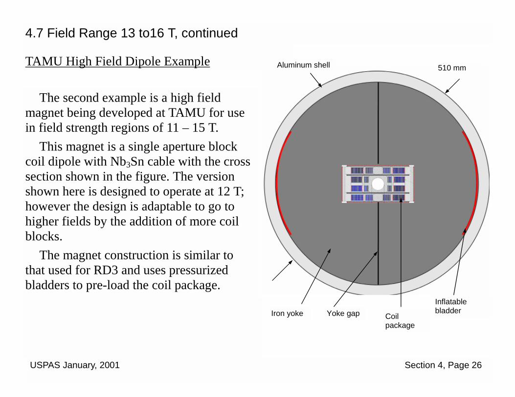
The second example is a high field magnet being developed at TAMU for use in field strength regions of 11 – 15 T.
This magnet is a single aperture block coil dipole with Nb3Sn cable with the cross section shown in the figure. The version shown here is designed to operate at 12 T; however the design is adaptable to go to higher fields by the addition of more coil blocks.
The magnet construction is similar to that used for RD3 and uses pressurized bladders to pre-load the coil package.
TAMU High Field Dipole Example
4.7 Field Range 13 to16 T, continued
510 mm Aluminum shell
Iron yoke Yoke gap Coil package
Inflatable bladder

USPAS January, 2001 Section 4, Page 27
This design requires that the ends of the center coil blocks be bent out of the plane of the coil in order to accommodate the beam tube, as shown in the figure.
The coil blocks that are above and below the beam tubes can be wound flat and thus avoid this complication.
However, in this presentation we will only consider the design of the 2-dimensional cross section of the cold mass and not include the design of the coil end support structure.
Beam tube representing coil aperture
Four innermost coil blocks bent out of the plane of the beam tube. (Outermost coil blocks not shown.)
4.7 Field Range 13 to 16 T, continued
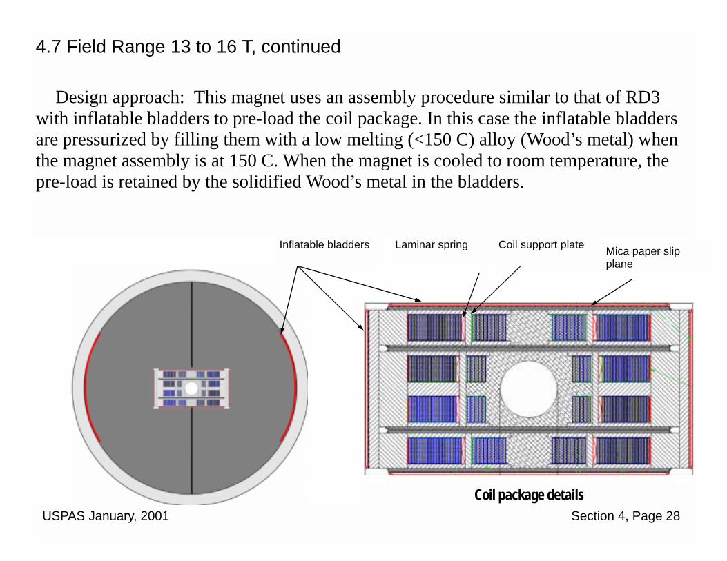
USPAS January, 2001 Section 4, Page 28
Design approach: This magnet uses an assembly procedure similar to that of RD3 with inflatable bladders to pre-load the coil package. In this case the inflatable bladders are pressurized by filling them with a low melting (<150 C) alloy (Wood’s metal) when the magnet assembly is at 150 C. When the magnet is cooled to room temperature, the pre-load is retained by the solidified Wood’s metal in the bladders.
4.7 Field Range 13 to 16 T, continued
Coil package details
Inflatable bladders Laminar spring Coil support plate Mica paper slip plane

USPAS January, 2001 Section 4, Page 29
As mentioned earlier, it is important to avoid too much normal stress on the Nb3Sn conductor. A feature of this TAMU magnet design is the method of handling the forces on each coil block by means of a “Stress management” system. Basically, each coil block is isolated in its own compartment and supported separately. Thus, the Lorentz force exerted on multiple coil blocks does not accumulate and this lowers the risk of conductor degradation.
The Lorentz force on each segment is transmitted to the magnet frame by the Inconel ribs to Inconel plates. This has been calculated to reduce the maximum stress on the conductor to about 1/3 of what would be obtained without the ribs. A laminar spring is used to preload on each block to get the initial elastic modulus high. The lower two figures show the stress distribution in the plates at zero and 16 T.
4.7 Field Range 13 to 16 T, continued Cable turns Laminar spring
Slip plane Inconel ribs and plates
Support force B = 0 T
B = 16 T
Lorentz force

USPAS January, 2001 Section 5, Page 1
SUPERCONDUCTING ACCELERATOR MAGNETS
An Introduction to Mechanical Design and Construction Methods Carl L. Goodzeit (BNL, ret.)
Note: Some of the material presented in this course was taken from: “Superconducting Accelerator Magnets”, an interactive CD ROM tutorial published by MJB Plus Inc.
(www.mjb-plus.com)
Section 5. Construction and Assembly

USPAS January, 2001 Section 5, Page 2
5. CONSTRUCTION AND ASSEMBLY OF AN ACCELERATOR DIPOLE (COSINE THETA TYPE)
This section is covered in Lesson 1.8 that is found on the CD-ROM “Superconducting Accelerator Magnets” that was supplied with the USPAS course.
The CD-ROM Tutorial shows assembly steps and videos of fabrication and assembly operations for an SSC dipole.

USPAS January, 2001 Section 6, Page 1
SUPERCONDUCTING ACCELERATOR MAGNETS
An Introduction to Mechanical Design and Construction Methods Carl L. Goodzeit ( BNL, ret.)
Note: Some of the material presented in this course was taken from: “Superconducting Accelerator Magnets”, an interactive CD ROM tutorial published by MJB Plus Inc.
(www.mjb-plus.com)
Section 6. Design Exercise using Finite Element Method
© 2001 Carl L. Goodzeit All rights reserved.

USPAS January, 2001 Section 6, Page 2
6.1 Overview of Mechanical Design Methods
Introduction In this discussion we address the mechanical analysis of the cold mass with
respect to the applied thermal and Lorentz loads in 2-dimensions. The mechanical design is primarily concerned with ensuring that the coil motion is
restrained sufficiently to prevent conductor displacement that will cause the magnet to quench. In this respect, magnet components are designed primarily on the basis of deflection under load rather than allowable stress.
For the case of dipoles (the principal type of magnet considered in this course), the horizontal resultant of the Lorentz forces is the principal force to be considered. We have seen examples of how these forces are handled for both cosθ and block or flat coil configurations. The same principal applies to all these cases, i.e., to prevent coil motion, a horizontal force is applied to the coil that is equal to or greater than the expected Lorentz force at operating conditions.

USPAS January, 2001 Section 6, Page 3
The restraining horizontal force can be applied by the following methods: Type 1. Self supporting collars for cosθ magnets in which the collar is structurally
adequate to take the horizontal force without exceeding a specified maximum deflection, usually ~0.06 mm. (Tevatron, HERA)
Type 2. Vertically split yoke with a gap, so that force is transmitted from the outer shell through the yoke to coil pack. (most other designs; Figure on left)
Type 3. Horizontally split yoke using a combination of the yoke stiffness and the shell tension; this acts much like a very stiff self supporting collar. (Figure on right)
There are some simple analytical techniques that can be applied to get a first order approximation for each of the designs; however, the main and most revealing analysis method is to use finite element stress analysis for these problems.
6.1 Overview of Mechanical Design Methods, continued.
Vertical yoke split
Horizontal yoke split
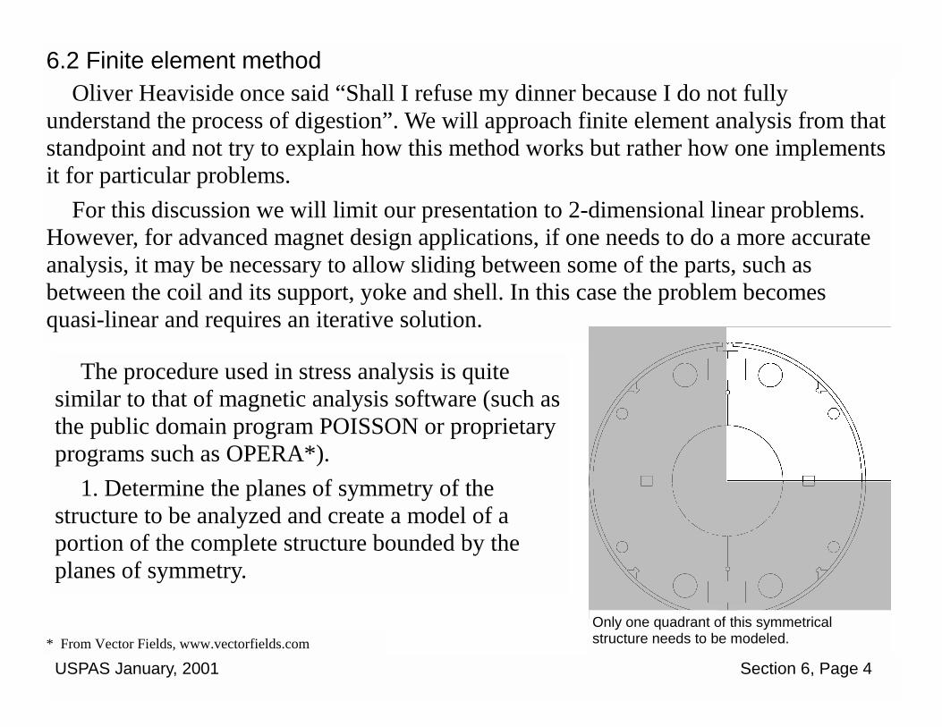
USPAS January, 2001 Section 6, Page 4
6.2 Finite element method Oliver Heaviside once said “Shall I refuse my dinner because I do not fully
understand the process of digestion”. We will approach finite element analysis from that standpoint and not try to explain how this method works but rather how one implements it for particular problems.
For this discussion we will limit our presentation to 2-dimensional linear problems. However, for advanced magnet design applications, if one needs to do a more accurate analysis, it may be necessary to allow sliding between some of the parts, such as between the coil and its support, yoke and shell. In this case the problem becomes quasi-linear and requires an iterative solution.
* From Vector Fields, www.vectorfields.com
The procedure used in stress analysis is quite similar to that of magnetic analysis software (such as the public domain program POISSON or proprietary programs such as OPERA*).
1. Determine the planes of symmetry of the structure to be analyzed and create a model of a portion of the complete structure bounded by the planes of symmetry.
Only one quadrant of this symmetrical structure needs to be modeled.

USPAS January, 2001 Section 6, Page 5
2. Divide each region in the model into a mesh or lattice of small elements. Usually these elements are rectangular, but they can also be triangular. The corners of the elements are called nodes and are used in stress analysis as the locations at which to apply boundary conditions and loads.
6.2 Finite element method, continued.
3. Define the properties of the material in each of these regions and assign the specific material to each region. These properties include (a) Elastic moduli in 3 directions (they would be different for orthotropic material), (b) Poisson’s ratio in 3 directions, and (c) the average thermal expansion coefficient in 3 directions. Density is also used since most programs will calculate the weight of the model and for advanced users it is required for dynamics problems.
4. Define the type of elements in each region, selecting from the various types of structural elements are available in the element libraries of the finite element software package. Examples are:
• 2-dimensional plane stress or plane strain quadrilateral elements for use in plane or axi-symmetric geometry.
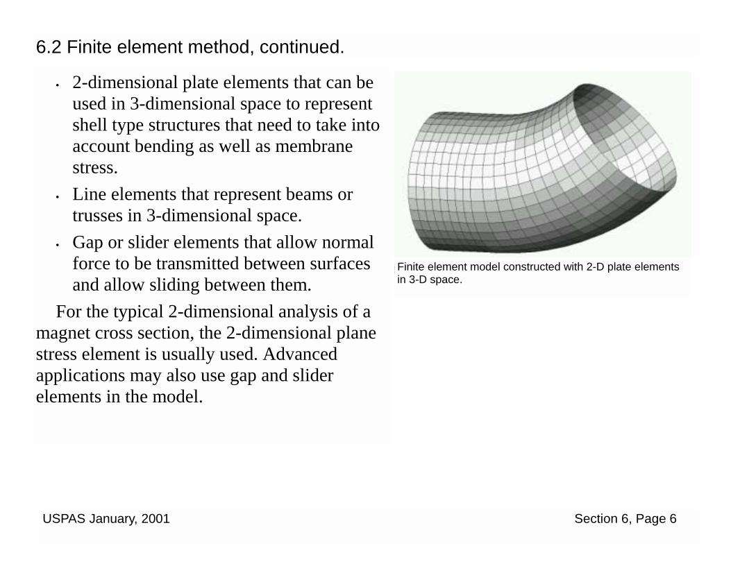
USPAS January, 2001 Section 6, Page 6
6.2 Finite element method, continued.
• 2-dimensional plate elements that can be used in 3-dimensional space to represent shell type structures that need to take into account bending as well as membrane stress.
• Line elements that represent beams or trusses in 3-dimensional space.
• Gap or slider elements that allow normal force to be transmitted between surfaces and allow sliding between them.
For the typical 2-dimensional analysis of a magnet cross section, the 2-dimensional plane stress element is usually used. Advanced applications may also use gap and slider elements in the model.
Finite element model constructed with 2-D plate elements in 3-D space.

USPAS January, 2001 Section 6, Page 7
5. Define the boundary conditions to be applied to the model. For example, the edges of symmetry of the model need to be constrained so that they can move only in the allowed directions. This is done by applying constraints to each node along the specific edge.
6.2 Finite element method, continued.

USPAS January, 2001 Section 6, Page 8
6.2 Finite element method, continued. 6. Apply the loads to the model. These can be a. Force vectors applied to specific nodes. b. Prescribed displacements applied to specific nodes. c. Pressure applied to sides of elements. d. Temperature difference from an initial reference temperature. Sometimes it is desirable to run each load case separately so that the effects can be
examined. If the problem is linear, the results can be superimposed to get the combined effect, but, if quasi-linear elements are used, superposition is not valid.
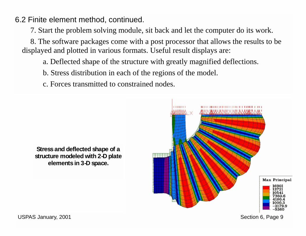
USPAS January, 2001 Section 6, Page 9
7. Start the problem solving module, sit back and let the computer do its work. 8. The software packages come with a post processor that allows the results to be
displayed and plotted in various formats. Useful result displays are: a. Deflected shape of the structure with greatly magnified deflections. b. Stress distribution in each of the regions of the model.
c. Forces transmitted to constrained nodes.
6.2 Finite element method, continued.
Stress and deflected shape of a structure modeled with 2-D plate
elements in 3-D space.

USPAS January, 2001 Section 6, Page 10
6.3 Design exercise: application to a 6.6 T magnet development. As a design exercise we will develop a structural design for a prototype dipole cold
mass similar to the SSC dipole. We will use simplified finite element models for the various stages of the development of the design.
We develop the structural design starting with support of the coil. The final coil geometry and the inside and outside diameter of the yoke are determined from the magnetic analysis. Thus, the dimensions of the collar are determined. Stainless steel collars are used (Nitronic 40, for reasons previously presented.)
For the purpose of this exercise, we will use a simplified analysis and model the collar as a single layer structural member and not as a spot welded pair.
A more precise analysis would take into account the two collars that are spot welded and that model would be more complicated. However, the structural response of the simplified model is quite close to the more detailed case. Pair of collar laminations spot welded together
to form a structural member. In this exercise only a single layer symmetrical collar will be
Spot weld

USPAS January, 2001 Section 6, Page 11
A B
As an additional simplification, the coil will not be included in the structural model. However, the loads produced by the coil (i.e. pre-stress and Lorentz force) will be applied to the model. In this exercise we will assume that the inner and outer coils, when collared, will have a compressive pre-stress of 83 MPa (12,000 psi). The assembly will be cooled down to 4.2 K and the Lorentz force at 6.6 T applied to the complete cold mass structure. We will then examine the structural response under these conditions.
6.3 Design exercise: continued.
The principal dimensions of the collar required for this design are shown in the figure.
Dimensions in mm: A - 67.82 E - 102.68 deg. B - 24.8 F - 35.86 deg. C - 37.92 D - 50.83
C
D
E F
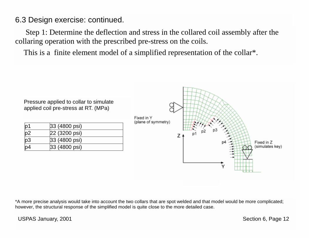
USPAS January, 2001 Section 6, Page 12
6.3 Design exercise: continued. Step 1: Determine the deflection and stress in the collared coil assembly after the
collaring operation with the prescribed pre-stress on the coils. This is a finite element model of a simplified representation of the collar*.
*A more precise analysis would take into account the two collars that are spot welded and that model would be more complicated; however, the structural response of the simplified model is quite close to the more detailed case.
p1 33 (4800 psi) p2 22 (3200 psi) p3 33 (4800 psi) p4 33 (4800 psi)
Pressure applied to collar to simulate applied coil pre-stress at RT. (MPa)
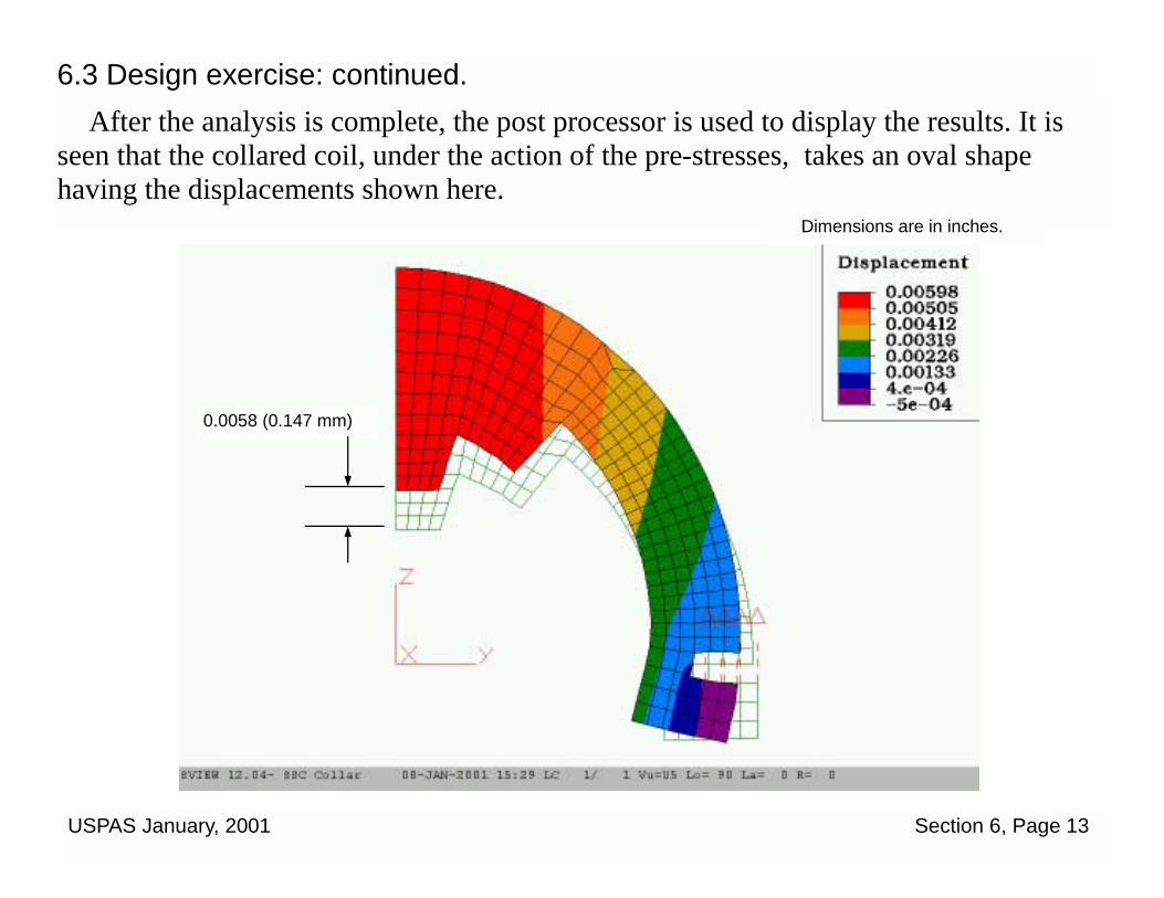
USPAS January, 2001 Section 6, Page 13
6.3 Design exercise: continued. After the analysis is complete, the post processor is used to display the results. It is
seen that the collared coil, under the action of the pre-stresses, takes an oval shape having the displacements shown here.
Dimensions are in inches.
0.0058 (0.147 mm)

USPAS January, 2001 Section 6, Page 14
Step 2: Fit collared coil assembly into the yoke and helium containment shell. We will examine the two different yoke configurations that were considered for the SSC dipole.
Option 1: Use a horizontally split yoke, apply pressure to squeeze the collared coil
into a circular shape, and clamp into the yoke with tensile stress in the shell. Pressure is applied to squeeze ovalized collar assembly into the yoke.
Weld to complete assembly
Horizontal yoke split
Finite element model constrained for horizontally split yoke. Shell is allowed to slide on yoke by using gap elements.
Fixed in Y
6.3 Design exercise: continued.

USPAS January, 2001 Section 6, Page 15
The Lorentz force can be resolved into horizontal and vertical components. The horizontal force tends to push the coils apart and acts on the coil support structure. In this simplified model we will apply the horizontal Lorentz force (FL) to the collar and yoke assembly to determine the structural response.
The figures below show the deflected shape and the maximum principal stress in the structure after the application of FL = 5000 lb/in and the thermal load for a temperature of 4.2 K. It is seen that the assembly shrinks and there is a 4 mil displacement of the yoke toward the mid-plane that would close up any gap there. The shell stress is moderate (16,440 psi, 113 MPa).
6.3 Design exercise: continued.
Inches psi
FL
0.014
0.0072
0.0041
16,440

USPAS January, 2001 Section 6, Page 16
6.3 Design exercise: continued. Option 2: Use a vertically split yoke which can apply a horizontal force directly to
the collared coil assembly by means of the tensile stress in the shell. Since the collared coil assembly becomes oval, it is not feasible to assemble this
directly into a vertically split yoke of the same nominal diameter as the collar. In order to compensate for the ovality of the collared coil assembly, and thus allow the yoke to fit precisely, the shape of the collar was modified as shown in the figure*.
* This work was done at FNAL [J. Strait, “Modifications to the Collar for the Vertically Split Yoke SSC Dipole Magnet”, FNAL Report TS-SSC 90-041, July 19, 1990.]
This modification allows the collared coil to fit in the vertically split yoke and allows the sides to be loaded in compression by pressing the shell in a horizontal direction and welding it.
weld

USPAS January, 2001 Section 6, Page 17
We apply the same loading conditions to this model as in the previous case. However, the boundary conditions are that the yoke is fixed in the Z-direction along its horizontal edge and it is free to move at the vertical plane. The result is shown in the figures.
This time the yoke tends to squeeze in towards the vertical split and other deflections are similar. The shell stress is slightly higher since the yoke does not help support the horizontal Lorentz force. Thus, it appears that either design choice is capable of supporting the Lorentz force on the coil with adequate rigidity.
6.3. Design exercise: continued.
0.0147
Inches psi
FL
0.00614
0.0033 18,630
USPAS January, 2001 Section 6, Page 18
6.3 Design exercise: continued. Discussion.
This exercise shows how finite element structural models can be used to develop the mechanical design for just about any type of magnet application. The finite element approach is most valuable however, for superconducting magnets since the Lorentz loads are quite high and the support of the coils are a primary consideration.
We have seen how effective a simple 2-D analysis of the cross section can be in achieving an understanding of the structural response of the structure to various types of loads.
It should be noted that most of the time spent on a finite element analysis is in the creation of the finite element structural model. Once this model has been defined satisfactorily and checked for completeness and consistency, it can be used repeatedly to make design iterations and vary the boundary conditions and loads.
The same procedures used in this example of the cosθ type dipole can be easily applied to other configurations such as the block coil and common coil design magnets that we have seen previously.
USPAS January, 2001 Section 6, Page 19
More information on proprietary finite element software can be found from the following sources:
ALGOR is a finite element structural analysis package and is the one that was used for the examples in this section.
www.Quickfield.com Quickfield is a combination (magnetostatic, electrostatic, thermal, and structural)
finite element package (2-D only) offered by Tera Analysis, Ltd. There is a free student version of the program that can be downloaded from their web site. However, this free version only permits models with up to 200 nodes, and thus, it is rather limited in what you can do with it. However, the procedures used are common to all finite element programs and thus it serves as a good introduction to actually performing such analyses.
www.ansys.com offers finite structural analysis software from ANSYS, Inc.
6.3 Design exercise: continued.

USPAS January 21, 2001 Section 7, Page 1
SUPERCONDUCTING ACCELERATOR MAGNETS
An Introduction to Mechanical Design and Construction Methods Carl L. Goodzeit (BNL, ret.)
Section 7. Problems
© 2001 Carl L. Goodzeit All rights reserved.

USPAS January 21, 2001 Section 7, Page 2
Problem 1. Coil End Forces
The figure shows a single layer in a common coil design magnet. A field plot of a cross section of a quadrant of the magnet shows that the field on the inner surface of the coil is 13 T. If it is assumed that the entire inner periphery of the coil sees this field then:
Calculate the following: A. End force (FE) acting on a the coil. B. Longitudinal stress in the coil section if the end is unsupported. C. Longitudinal stress if the field is 16 T.
FE

USPAS January 21, 2001 Section 7, Page 3
Problem 2. Initial Strain
The assembly shown simulates a yoke enclosed in a helium containment shell. The shell has been pressed against the yoke and welded. After the assembly has cooled to 293 K, the strain in the shell was measured and found to be 0.000666 from the shrinkage of the weld zones. (Use 293 K material properties.) 1.What is the normal pressure , p,
between the shell and yoke when the assembly is at 293 K?
2.If the assembly is cooled to 4.2 K, what is the force (F) per mm between the upper and lower yoke halves?
Shell, 304 stainless steel
Yoke, iron
Weld
50
100
7
F
p
Dimensions in mm

USPAS January 21, 2001 Section 7, Page 4
Two types of stainless steel alloys (Alloy A and Alloy B) have the following composition in weight %:
Element Alloy A Alloy B Cr 19.36 18.95 Ni 7.81 9.5 Mn 1.19 1.5 Si 0.6 0.75 N 0.19 0 C 0.025 0.05 Fe Bal. Bal. Mo 0.032 0 Nb 0 0.5
Problem 3. Stainless steel magnetic permeability
Estimate the expected room temperature magnetic permeability of each of these alloys
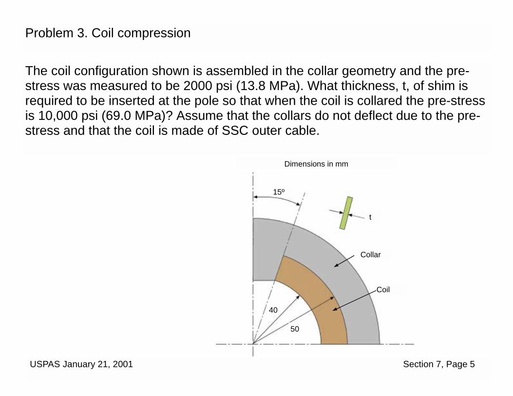
USPAS January 21, 2001 Section 7, Page 5
Problem 3. Coil compression
The coil configuration shown is assembled in the collar geometry and the pre-stress was measured to be 2000 psi (13.8 MPa). What thickness, t, of shim is required to be inserted at the pole so that when the coil is collared the pre-stress is 10,000 psi (69.0 MPa)? Assume that the collars do not deflect due to the pre-stress and that the coil is made of SSC outer cable.
t
15º
40
50
Collar
Coil
Dimensions in mm

USPAS January 21, 2001 Section 7, Page 6
The diagram shows a simplified version of an RD3 type magnet assembly. It was assembled with a 45 mm thick 6061 aluminum shell and pre-loaded so that the shell tension is 3.6e6 N/m at 293 K. The tension increases to 6.36e6 N/m at 4.2 K.
Estimate the outward deflection, d, of the coil at: A: 13 T central field B. 16 T central field
Problem 4. Magnet Assembly Pre-loads
Shell
Yoke
Key
Coil
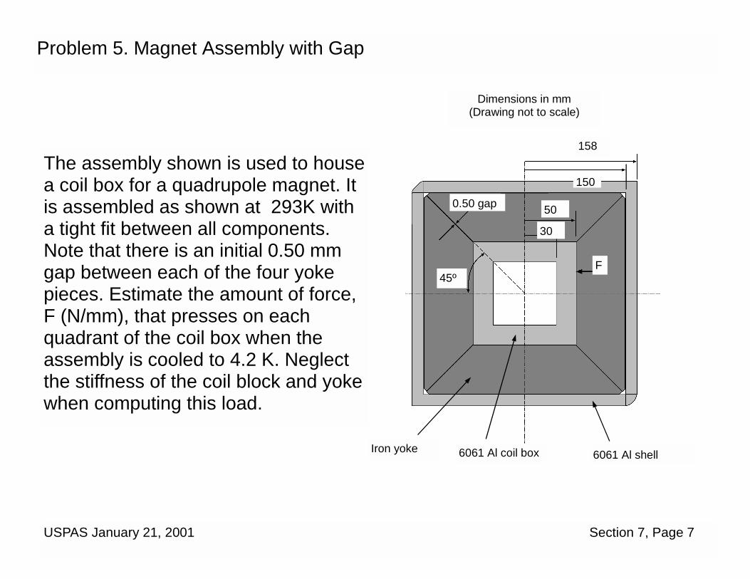
USPAS January 21, 2001 Section 7, Page 7
F
158
150
30
50
45º
0.50 gap
6061 Al shell 6061 Al coil box Iron yoke
Dimensions in mm (Drawing not to scale)
The assembly shown is used to house a coil box for a quadrupole magnet. It is assembled as shown at 293K with a tight fit between all components. Note that there is an initial 0.50 mm gap between each of the four yoke pieces. Estimate the amount of force, F (N/mm), that presses on each quadrant of the coil box when the assembly is cooled to 4.2 K. Neglect the stiffness of the coil block and yoke when computing this load.
Problem 5. Magnet Assembly with Gap

USPAS January 21, 2001 Section 7, Page 8
Solutions to Problems
Problem 1: Using the dimensions given for the single layer coil we can compute the end force from the magnetic pressure (p) acting on the inside coil at 13 T. Thus,
2 22
0
B 13p 6.728e07 N/m (9760 psi.)2 2 1.256e 06
= = =µ × −
A. The area, A, of the inside of the coil turn on which the pressure acts is A= 10 × 70 = 700 mm2 and thus the force acting on each half of the coil is 700 × 6.728e07 × 1e-06 = 47,094 N (10589 lb.)
B. Since the area of the coil section is 10 × 80 = 800 mm2 the tensile stress acing on the coil section is 47094/800/2 = 29.4 MPa (4270 psi.) when the coil end is unsupported.
C. At 16 T, the coil stress is 29.4 × (16/13)2 = 44.6 MPa (6450 psi.)
Problem 2: The following data for the shell and yoke material is obtained from the Material Properties Data: Procedure: Determine the force per unit of axial length , F, in the shell from the initial strain condition. The horizontal (or vertical) resultant of the pressure, p, between the shell and yoke ( at radius, R) must balance this force. The stress in the shell from the initial strain condition is 0.000666 × 193 = 128 MPa (18,640 psi.) The tensile force in the shell is F = 128 × 7 = 897 N/mm (5120 Lb/in.) Thus, p = F/R = 897/100 = 8.97 MPa (1300 psi.)
Material ∆L/L0 293 - 4.2 K E (GPa), (psi)
304 SS 0.00284 193 (27.9e6)
Yoke iron 0.00194 207 (30.0 e6)

USPAS January 21, 2001 Section 7, Page 9
Problem 2, continued 2. Procedure: To determine the force in the shell when the assembly is cooled to 4.2 K, we need to find the incremental strain in the shell when it shrinks against the iron yoke. From this we get the incremental stress in the shell and then the incremental force which is added to the initial force to get the total force in the shell which also acts to compress the two yoke halves. The shell circumference is 628.3 mm at its inside diameter. Thus, at 4.2 K it would shrink 0.00284 × 628.3 = 1.784 mm. However, it is restrained by the yoke which shrinks 0.00194 × 628.3 = 1.219 mm at its outside diameter. The incremental shrinkage of the shell is therefore 1.784 - 1.219 = 0.565 mm and the incremental strain is 0.565/628.3 = 0.00090. The incremental stress is 0.00090 × 192 x 1000 = 172.8 MPa. The incremental force is therefore 172.8 × 7 = 1210 N/mm. The total force is therefroe 897 + 1210 = 2109 N/mm (12,000 lb/in) which acts to compress the yoke halves.
Problem 3: Procedure: The Schaeffler diagram on pg. 6 of the Material Properties Data can be used to estimate the ferrite content of each of these alloys. Then the permeability can be estimated by a visual interpolation from the curve on pg. 6. Thus, Cr Equivalent = (Cr+Mo+1.5 Si+0.5 Nb) and Nickel Equivalent = (Ni+30(C+N)+0.5Mn). With the composition data for alloy A and alloy B shown in the table the following values are interpolated:
Cr Ni Ferrite µ Alloy A 20.3 14.9 0.02 1.1 Alloy B 20.3 11.8 0.1 2.1

USPAS January 21, 2001 Section 7, Page 10
Problem 4: Procedure: The stress strain relation for a section of coil made with SSC outer cable is given in the Material Properties Data. This relation is used to compute the strain necessary to get 69 MPa compressive stress. This strain used to obtain the compressed coil length at that stress. The shim thickness is determined by taking the difference of the coil length at the initial condition between that at the 69 MPa stress level. The stress strain relation is:
6 2 8.0 3400 1.10 10 MPaσ = + ε + × εA coil section with an inner radius of 40 mm and an outer radius of 50 mm and an angle of 75° has a nominal length of 58.9 mm. First we determine the coil strain at an initial stress of 13.8 MPa. This can be done quickly with EXCEL goal solving and we obtain e = 0.001221. In a similar manner the strain required for 69 MPa is 0.00606. Therefore the change in strain from the initial condition to 69 MPA is 0.004839. This, multiplied by the length of the coil gives the required shim thickness. Thus, 0.004839 × 58.9 = 0.285 mm.
Problem 5: Procedure: In the configuration shown, the shell is already in tension at 4.2 K and loads the coil with a force of 6360 N/mm per coil quadrant. Thus, the shell has an initial strain and the strain will not increase (hence, the deflection) until the load applied to the structure by the coils exceeds the shell tension. We need the elastic modulus of the shell material, 6061 aluminum, which is 79 GPa (11.4e6 psi) at 4.2 K. First we will compute the force exerted by the coils at 13 T using the result already obtained in problem 2. Thus, the pressure , p, is:
2 22
0
B 13p 6.728e07 N/m (9760 psi.)2 2 1.256e 06
= = =µ × −
A. The force on an 80 mm wide coil is 6.728e7 × 80 = 5390 N/mm which is less than the pre-load of 6360 N/mm and thus there is nominally no coil deflection.
B. At 16 T, the coil force is 8149 N/mm. The excess force over the pre-load is 8149 - 6360 = 1789 N/mm. This is taken by the shell and produces an incremental stress of 1789/45 = 39.8 MPs (5760 psi). The incremental strain is 39.8/79 = 0.00050. The length of the shell at its center line is 330 +22.5 = 352.5 mm and thus the radial deflection is 352.5 × 0.00050 = 0.177 mm which is the outward deflection of the coil.

USPAS January 21, 2001 Section 7, Page 11
Problem 5: Procedure: Force is transmitted to the coil box by the thermal shrinkage of the shell as long as the gap stays open. If the nominal gap distance is d, then the horizontal motion of the coil box (from the c/l) necessary to close the gap is d/sin 45°. We use the following mechanical properties:
Material ∆L/L0 293 - 4.2 K E (GPa), (psi)
Al 6061 0.00386 79 (11.5e6)
Yoke iron 0.00194 207 (30.0 e6)
The following dimensions are from the diagram: mm Inches Shell thickness 8 0.315 Shell distance from inside to c/l 150 5.9 yoke width 100 3.932 box width 50 1.986 gap nominal, d 0.16 0.006 gap, horizontal 0.22 0.0084853
The unrestrained shell shrinks (from the c/l): e0 = 8 × 0.00386 = 0.5785 mm The unrestrained iron shrinks (from the c/l): e1 = (100 - 50) x 0.00194 = 0.1938 mm The coil box shrinks e2 = 50 x 0.00386 = 0.1947 mm [Note that this is less than the horizontal gap; thus force will be transmitted to the coil box.] Thus, when cold, the net deformation in the shell is: e0 - e1 -e2 = 0.2155 mm The strain in the shell is therefore 0.00192 which give a shell stress of 152 MPa (22,100 psi.) The net force on the box is therefore 0.31 x 152 = 1220 N/mm ( 6850 lbs/in). However, this does not take into account the compressibility of the box and the yoke under this load. That reduces the strain in the shell and therefore the load seen by the box.

USPAS January, 2001 Page 1 Rev. 02/01
Superconducting Accelerator Magnets
An Introduction to Mechanical Design and Construction Methods
Carl L. Goodzeit (BNL, ret.)
MATERIAL PROPERTIES REFERENCE DATA This supplement contains general reference data for some materials that are commonly used in superconducting magnets. This compilation will be needed for examples given in the lecture. It should also be a handy reference for your future consideration of magnet mechanical designs.
1. Mechanical Properties
a. Metals and alloys
b. Plastics and Composites
c. Rutherford cable coil sections
2. Stainless steel composition effects
a. Schaeffler Diagram
b. Permeability vs. ferrite content
3. Thermal contraction data
a. Metals and alloys
b. Plastics and composites
c. Rutherford cable coil sections
4. Radiation Resistance of Plastics, Composites and Films
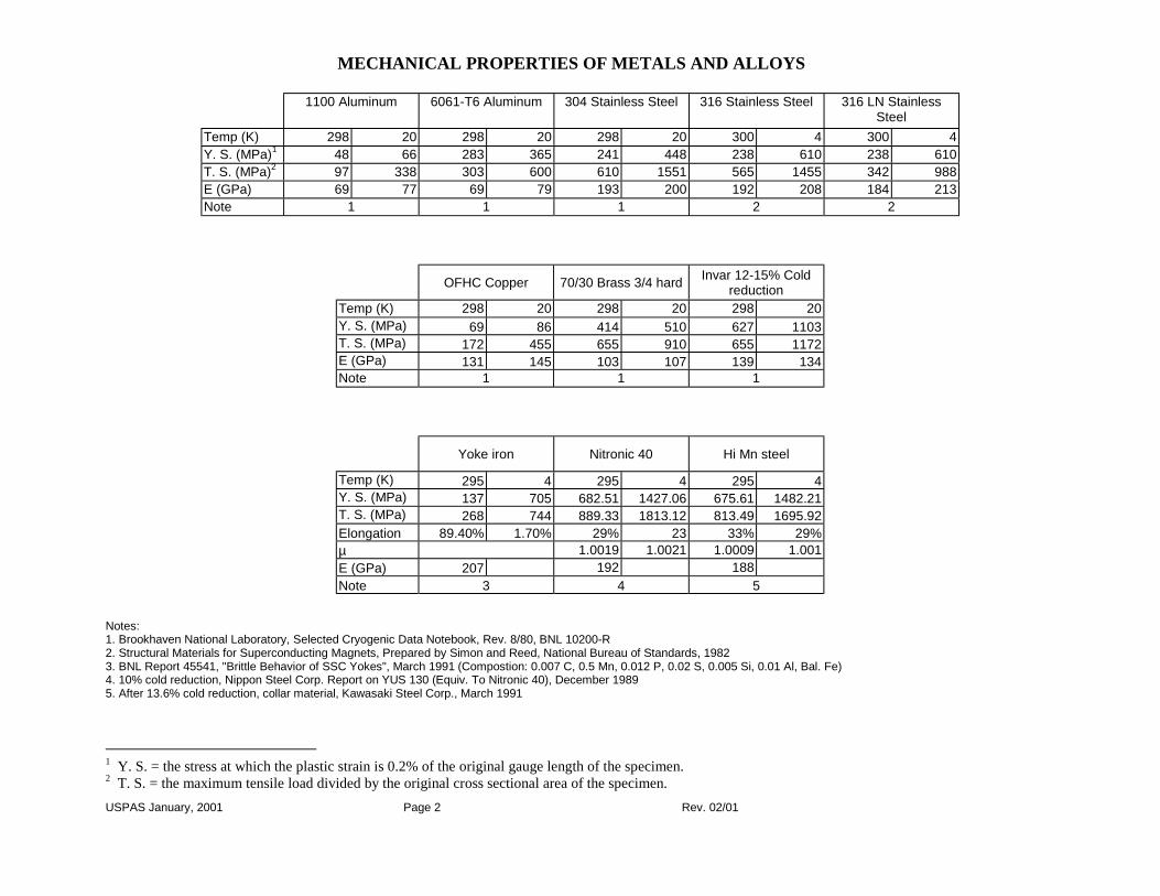
USPAS January, 2001 Page 2 Rev. 02/01
MECHANICAL PROPERTIES OF METALS AND ALLOYS
Notes: 1. Brookhaven National Laboratory, Selected Cryogenic Data Notebook, Rev. 8/80, BNL 10200-R 2. Structural Materials for Superconducting Magnets, Prepared by Simon and Reed, National Bureau of Standards, 1982 3. BNL Report 45541, "Brittle Behavior of SSC Yokes", March 1991 (Compostion: 0.007 C, 0.5 Mn, 0.012 P, 0.02 S, 0.005 Si, 0.01 Al, Bal. Fe) 4. 10% cold reduction, Nippon Steel Corp. Report on YUS 130 (Equiv. To Nitronic 40), December 1989 5. After 13.6% cold reduction, collar material, Kawasaki Steel Corp., March 1991
1 Y. S. = the stress at which the plastic strain is 0.2% of the original gauge length of the specimen. 2 T. S. = the maximum tensile load divided by the original cross sectional area of the specimen.
1100 Aluminum 6061-T6 Aluminum 304 Stainless Steel 316 Stainless Steel 316 LN Stainless Steel
Temp (K) 298 20 298 20 298 20 300 4 300 4 Y. S. (MPa)1 48 66 283 365 241 448 238 610 238 610 T. S. (MPa)2 97 338 303 600 610 1551 565 1455 342 988 E (GPa) 69 77 69 79 193 200 192 208 184 213 Note 1 1 1 2 2
OFHC Copper 70/30 Brass 3/4 hard Invar 12-15% Cold
reduction Temp (K) 298 20 298 20 298 20 Y. S. (MPa) 69 86 414 510 627 1103 T. S. (MPa) 172 455 655 910 655 1172 E (GPa) 131 145 103 107 139 134 Note 1 1 1
Yoke iron Nitronic 40 Hi Mn steel
Temp (K) 295 4 295 4 295 4 Y. S. (MPa) 137 705 682.51 1427.06 675.61 1482.21 T. S. (MPa) 268 744 889.33 1813.12 813.49 1695.92 Elongation 89.40% 1.70% 29% 23 33% 29% µ 1.0019 1.0021 1.0009 1.001 E (GPa) 207 192 188 Note 3 4 5

USPAS January, 2001 Page 3 Rev. 02/01
MECHANICAL PROPERTIES OF SOME PLASTICS AND COMPOSITES
Nylon Type 101 TFE Teflon 66.2 % crystallinity
Temp (K) 300 77 300 20 Y. S. (MPa) 51 241 14 110 T. S. (MPa) 72 241 28 110 E (GPa) 2.8 8.3 0.7 4.1 Note 1 1
MECHANICAL CHARACTERIZATION OF GIO-CR AND G11-CR MANUFACTURER A-PILOT PLANT (AVERAGE OF AT LEAST THREE SPECIMENS) Note 2
Notes: 1. Brookhaven National Laboratory, Selected Cryogenic Data Notebook, Rev. 8/80, BNL 10200-R 2. Data from ca. 1960, Source Unknown
Shear strength Shear strength G10-CR Young's Modulus (E) Poisson's ratio, ν Tensile strength Compressive strength Tensile failure
strain (short beam) (Guillotine)
Temp. Warp Fill Warp Fill Warp Fill Warp Fill Normal Warp Fill Warp Fill Warp Fill (K) (Gpa) (Gpa) (MPa) (MPa) (MPa) (MPa) (MPa) (%) (%) (MPa) (MPa) (MPa) (MPa)
295 28 22.4 0.15 0.144 415 257 375 283 420 1.75 1.55 60 45 42 76 33.7 27 0.19 0.183 825 459 334 557 693 3.43 2.53 131 93 61 73
4 35.9 29.1 0.211 0.21 862 496 862 598 749 3.67 2.7 105 73 79 G11-CR
295 32 25.5 0.157 0.146 469 329 396 315 461 1.82 1.73 72 45 41 76 37.3 31.1 0.223 0.214 827 580 804 594 799 3.21 2.85 120 92 57 57
4 139.4 32.9 0.212 0.215 872 553 730 632 776 3.47 2.67 89 56 57

USPAS January, 2001 Page 4 Rev. 02/01
MECHANICAL PROPERTIES OF RUTHERFORD CABLE COIL SECTIONS The stress-strain curves shown below were obtained by compressing samples of molded coil sections of SSC inner and outer coils and measuring the stress (force/area) and the strain (∆L/L0 ). Because molded coils have a certain amount of looseness under zero load, the zero strain condition was taken at 15 MPa and 8 MPa for the inner and outer coils respectively. The stress (σ) vs. strain (ε) relation is given by the following least squares fit of the data:
6 2
6 2
Inner coil: 15.0 5100 1.10 10 MPaOuter coil: 8.0 3400 1.10 10 MPa
σ = + ε + × ε
σ = + ε + × ε
Coil stress vs. strain
0
10
20
30
40
50
60
70
80
0 0.001 0.002 0.003 0.004 0.005 0.006 0.007Compressive strain
Stre
ss, M
Pa
Inner CoilOuter Coil

USPAS January, 2001 Page 5 Rev. 02/01
2. STAINLESS STEEL COMPOSITION EFFECTS
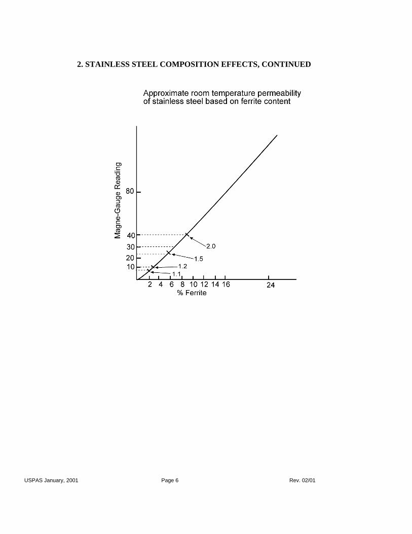
USPAS January, 2001 Page 6 Rev. 02/01
2. STAINLESS STEEL COMPOSITION EFFECTS, CONTINUED

USPAS January, 2001 Page 7 Rev. 02/01
3. THERMAL CONTRACTION DATA Source: “Thermal Contraction Measurements Relative to Titanium Silicate From 293 K to 4.2 K”,
BNL Magnet Division Note 455-15 (SSC-MD-287), July 1992
Note: The thermal contraction of titanium silicate in the range 293 K to 4.2 K is virtually zero. Thus, strain gauges can be used to measure thermal contraction if a set of identical gauges is mounted on the sample to be tested and also on a piece of titanium silicate. The resistance change from 293 K to 4.2 K is measured for each gauge; if the change for the titanium silicate is subtracted from that for the test sample, the result is proportional to the thermal strain of the material in that range. Certain materials tested have orthotropic contraction characteristics (e.g. composite materials and molded coil samples). In this way, thermal contraction in three orthogonal directions was determined for such materials.
3.1 METALS AND ALLOYS (293K TO 4.2K)
MATERIAL 0
L / Lε = ∆ COMMENT
Nitronic 40, SSC collar material 0.00241 High strength stainless steel used for collars HiMn, collar material (KHMn30L) 0.00157 High strength stainless steel used for collars Naval brass 0.00347 Shims, spacers, etc HiMn, 4mm thick 0.00156 HiMn, 10 mm thick 0.00154 Aluminum, 6061T6 0.00386 Collars, spacers Stainless steel, 304 0.00284 Helium shell Stainless steel, 316 0.00282 Various parts Invar 0.00044 For reference Stainless steel, A286 0.00277 Strain gauge beams Yoke iron, 1/4 inch 0.00194 Yokes Yoke iron, 16 gauge 0.00194 Copper, OFHC 0.00312
3.2 PLASTICS AND COMPOSITES (293K TO 4.2K)
MATERIAL 0
L / Lε = ∆ COMMENT
Spaulrad, azimuthal 0.00195 Candidate material for coil end parts Spaulrad, longitudinal 0.00261 “ Spaulrad, transverse 0.00218 “ Lexan, azimuthal 0.01202 For reference Lexan, longitudinal 0.01191 “ Lexan, transverse 0.00945 “ RX630, azimuthal 0.00316 RHIC insulator/ spacers

USPAS January, 2001 Page 8 Rev. 02/01
RX630, longitudinal 0.00346 “ RX630, transverse 0.00326 “ G10, azimuthal 0.00247 Insulators and other parts G10, longitudinal 0.00256 “ G10, transverse 0.00240 “ Ultem 2200, azimuthal 0.00605 RHIC support posts, final Ultem 2200, longitudinal 0.00643 “ Ultem 2200, transverse 0.00570 “ Ultem 2100, azimuthal 0.00740 RHIC support posts, preliminary Ultem 2100, longitudinal 0.00732 “ Ultem 2100, transverse 0.00639 “ RTV, Silicone cement 0.01623 Bulk adhesive Teflon, longitudinal 0.01742 For reference Teflon, transverse 0.01367 “ Torlon, transverse 0.00507 Possible for coil end parts Torlon, longitudinal 0.00621 “ Green putty (epoxy-glass mixture) 0.00340 Filler material (glass powder+epoxy) Nylon, azimuthal 0.01336 For reference Nylon, longitudinal 0.01742 “ Nylon, transverse 0.01367 “
3.3 RUTHERFORD CABLE COIL SECTIONS (293K TO 4.2K) Note: A is azimuthal direction, L is longitudinal direction and R is radial.
MATERIAL 0
L / Lε = ∆ TYPE OF CABLE INSULATION WRAP
SSC dipole inner coil, K-A 0.00563 Kapton wrap with adhesive SSC dipole inner coil, K-L 0.00262 “ SSC dipole inner coil, K-R 0.00418 “ SSC dipole inner coil, G-A 0.00511 Fiberglass cloth impregnated with epoxy SSC dipole inner coil, G-L 0.00247 “ SSC dipole inner coil, G-R 0.00395 “ SSC dipole outer coil, K-A 0.00626 Kapton wrap with adhesive SSC dipole outer coil, K-L 0.00249 “ SSC dipole outer coil, K-R 0.00444 “ SSC dipole outer coil, G-A 0.00498 Fiberglass cloth impregnated with epoxy SSC dipole outer coil, G-L 0.00257 “ SSC dipole outer coil, G-R 0.00415 “

USPAS January, 2001 Page 9 Rev. 02/01
4. RADIATION RESISTANCE OF PLASTICS, COMPOSITES AND FILMS Source: A. Spindel, “Report on the Program of 4 K Irradiation of Insulating Materials for the Superconducting Super Collider”, Draft Report, July 8, 1993 Several “radiation resistant” organic materials that were being evaluated for use in the superconducting magnets for the SSC were tested at 4 K to determine the effects on radiation exposure to their mechanical properties. The irradiation was performed at General Atomics in San Diego, CA with a beam from an electron accelerator with a dose of up to 109 rads except for films in which case the dose was 3.7 x 10⁹ rads. All tests were performed nominally at 4 K and the maximum temperature of any sample did not exceed 20 K. Mechanical tests were performed on these materials prior to and after irradiation. The mechanical tests were also done at 4 K. It is believed that the composite materials received a short beam shear and flexure test based on ASTM D2344-84. Also, the adhesives were tested in lap shear by gluing them to 0.032 inch thick 6061-T6 aluminum backing plates. All other materials were tested in tension. Table 1 lists the materials that were selected for these tests. The results of the mechanical tests before and after the radiation exposure are listed in Table 2. The values shown are averaged for a group of specimens. The data shown in Table 2 includes the ultimate shear-flexure strength (for composites) and the corresponding elastic moduli and displacement at failure. Resins and films data is tensile strength, elastic modulus and displacement or strain at failure. The lap-shear strength of the adhesives is listed.

USPAS January, 2001 Page 10 Rev. 02/01
TABLE 1 – SELECTED MATERIALS
Composites, Resins and Filled Systems
Material Vendor Dose (rads) Spaulrad Spaulding Composites 109 CTD101G CTD 109 Cryorad AlliedSignal 108,109 PEEK Victrex 108,109 VTEMI UDD-FIM 108,109 Ultem2300 GE 108,109 VespelSPA DuPont 109 Torlon5030 Amoco 109 Isary15X Isonova 109 Ultem6200 GE 108,109 Envex5630 Rodgers Corp. 108,109 CP1525 Creative Pulltrusions 108 CP1625 Creative Pulltrusions 108 Araldit/hardenr Ciba-Geigy 109 TE630 Permaglass 109 ME730 Permlaglass 109
Films
Material Vendor Dose (rads) Kapton H DuPont 109 Kapton HA DuPont 109 Kapton LT DuPont 109 Kapton HN DuPont 109 Kapton XMPI DuPont 109 Apical NP Allied Signal .. 109 Apical AV Allied Signal 109
Adhesives
Material Vendor Dose (rads) XMPI DuPont 109 Modified XMPI DuPont 109 CTD 105 CTD 109 Cryorad Allied Signal 109 3P Sheldahl 109 Modified 3P Sheldahl 109 EX 1508 Bryte 109 5575-2 BASF 109 E 388D BP Chemicals 109 EP0316 Isovolta 109 EP VP 1037/1 Isovolta 109

USPAS January, 2001 Page 11 Rev. 02/01
TABLE 2 - RESULTS OF MECHANICAL TESTS
Composites
AISS (ksi) Modulus (Msi) Dis 1 @ fail (in) Material 0 108 109 0 108 109 0 108 109 Spaulrad 9.62 ------- 10.3 3.415 ------- n.c. 0.042 ------- n.c. ME 730 12.0 ------- n.c. 2.04 ------- 2.34 0.034 ------- 0.031 CP 1625 5.54 n.c. ------- 2.01 2.49 ------- .030 0.028 ------- CP 1525 4.36 n.c. ------- 1.71 2.06 ------- 0.030 n.c. ------- Cryorad P 4.02 4.60 n.c. 2.41 2.66 n.c. 0.044 n.c. n.c. TE 630 13.6 ------- n.c. 3.74 ------- n.c. 0.048 ------- n.c. VTEM 2 9.49 n.c. n.c. 2.55 3.24 n.c. 0.054 n.c. n.c.
Resins and Filled Systems
Strength (ksi) Modulus (Msi) Dis @ fail (in) Material 0 108 109 0 108 109 0 108 109
Ultem 2300 61.9 n.c. n. c 1.20 1.28 n.c 0.016 n.c. n.c. Ultem 6200 32.7 n.c. 49.3 0.796 0.853 1.02 0.013 n.c. 0.016 PEEK 59.0 62.7 n.c. 1.09 1.34 n.c. 0.016 n.c. 0.015 CTD IOIG 33.5 ------- n.c. 1.98 ------- 2.08 0.007 ------- 0.004 Ves el SP 1 26.7 ------- 21.8 0.64 ------- 0.68 0.026 ------- 0.021 Araldit 21.6 ------- n.c. 2.40 ------- 2.08 0.006 ------- n.c. Envex 5630 40.3 57.14 n.c. 1.04 n.c. n.c. 0.025 .032 n.c. Torlon503O 62.3 ------- 58.1 1.15 ------- 1.26 0.035 ------- 0.030 Isa 115X 45.0 ------- 48.4 0.722 ------- 0.816 0.021 ------- 0.019
Adhesives
Strength (ksi) Strength (ksi) Material 0 109 Material 0 109
Cryorad 1.15 n.c. CTD 105 1.88 n.c. EX1508 1.63 1.81 V388/D 2.37 1.78 m3P/LT 1.33 n.c. CI/RCI 1.64 n.c. m3P/NP 2.65 1.88 RCI/RCI 1.44 n.c. m3P/VN * 2.16 n.c. XCI/XRCI 1.59 n.c. 5575-2/1 2.22 1.83 EPVP1037 2.07 n.c. 5575-2/2 2.03 1.69 EP0316 1.03 n.c.
Films
Strength (ksi) Modulus (Msi) Strain @ fail Material 0 109 0 109 0 109
Kapton HA 50.2 44.2 1.30 0.84 0.0348 0.0452 Kapton HN 74.1 42.1 1.75 1.00 0.0273 n.c. Kapton H 60.1 52.5 1.66 1.03 0.0335 n.c. Kapton LT 34.7 n.c. 1.03 n.c. 0.0345 n.c. Apical AV 73.8 51.0 1.82 0.968 0.0525 n.c. Apical NP 67.5 59.8 1.87 1.37 0.0461 0.0367