an explicit method for compressible flow simulation with...
TRANSCRIPT

An Explicit Method forCompressible Flow
Simulation with Regards toFluid-Motion Coupling
Jan Krautter
Born 11th March 1992 in Schorndorf
19th January 2016
Master’s Thesis Mathematics
Prof. Dr. Michael Griebel
Prof. Dr. Marc Alexander Schweitzer
Institute for Numerical Simulation
Mathematisch-Naturwissenschaftliche Fakultät der
Rheinischen Friedrich-Wilhelms-Universität Bonn

Contents
1 Introduction 3
2 An explicit compressible flow solver 72.1 The compressible Navier-Stokes equations . . . . . . . . . . . 72.2 A short review of existing methods . . . . . . . . . . . . . . . 92.3 The MacCormack scheme in fluid dynamics . . . . . . . . . . 112.4 Boundary conditions . . . . . . . . . . . . . . . . . . . . . . . 132.5 Stability . . . . . . . . . . . . . . . . . . . . . . . . . . . . . . 172.6 Parallelization . . . . . . . . . . . . . . . . . . . . . . . . . . . 182.7 An overview of the full algorithm . . . . . . . . . . . . . . . . 19
3 Geometry representation 233.1 The level set method . . . . . . . . . . . . . . . . . . . . . . . 233.2 Geometry import via the stl file format . . . . . . . . . . . . . 253.3 Comparison to the flag-field . . . . . . . . . . . . . . . . . . . 26
4 Simulation of moving objects 294.1 Adjusting the boundary conditions . . . . . . . . . . . . . . . 294.2 Moving geometries with a prescribed velocity . . . . . . . . . 314.3 Translation vs. rotation . . . . . . . . . . . . . . . . . . . . . 334.4 Bidirectional coupling . . . . . . . . . . . . . . . . . . . . . . 34
5 Example results 375.1 First Tests . . . . . . . . . . . . . . . . . . . . . . . . . . . . . 375.2 A benchmark problem . . . . . . . . . . . . . . . . . . . . . . 425.3 A physical problem . . . . . . . . . . . . . . . . . . . . . . . . 525.4 Unidirectional fluid-motion coupling . . . . . . . . . . . . . . 565.5 Bidirectional coupling . . . . . . . . . . . . . . . . . . . . . . 65
6 Outlook 73
Literature 79
1

2 CONTENTS

Chapter 1
Introduction
The physical understanding of processes involving flowing gases and/or liquids,so-called fluids is a field of vast theoretical interest, as well as many practicalapplications. The corresponding differential equations however, still pose ahuge challenge, as of today. Even in the most favourable conditions, they resistany attempt at proving global solutions and for complex problems, explicitsolutions in closed form are out of the question, anyway. On the other hand,physical experiments, often conducted in huge wind or water channels, arevery expensive and lack the kind of visualization and evaluation possibilitiesof mathematical solutions. Designing robust and accurate numerical methodsto approximate solutions, and cover the middle ground between these twoextremes, preferably establishing a positive feedback loop with either of them,thus, becomes all the more important. On the numerical side, flows aroundstatic geometries are by now comparatively well understood in both theincompressible, as well as the compressible case, at least in the laminar flowregime. For higher Reynolds numbers, turbulent phenomena still cause a lotof headache. The advent of ever faster computer hardware and techniquessuch as the large-eddy simulation, however, push the boundaries very fastin this respect, so it seems like it might only be a matter of time, untileven very complex simulations of today’s standard might be handled rathereasily. There is a whole different class of fluid problems, though, that stillhas many theoretical, as well as practical challenges ahead, despite manyinteresting applications and the ever increasing interest in it. In the mostgeneral sense, we are talking about flows, involving geometries, that evolveover time, either by having some parts of the geometry that are movingand/or rotating, like with a turbine or an engine, or even more complex, byhaving flexible or otherwise deforming objects, whose shape is dependant onthe flow surrounding them. The most prominent example, that showcases theimportance of these sorts of problems, until today, remains the collapse ofthe Tacoma Narrows Bridge in 1940, due to unforeseen oscillations caused bysuch fluid-structure interaction (FSI). Another take on the difficulty of such
3

4 CHAPTER 1. INTRODUCTION
problems, is the slightly ironic fact, that a paper air plane is, at least in someregards, actually much more difficult to understand and simulate, than a realaircraft. One huge area of applications, that we will come back to, in thecourse of this thesis, is the biological world, most prominently represented bythe flight of birds and/or insects. Quite obviously, a simulation solely basedon static obstacle geometry can only describe such a complex process, in avery limited way.
For the course of this thesis, keeping these complex problems as a motivationin the back of our mind, we want to first look at more basic examples of thisclass, restricting ourselves to the first case of purely moving geometries, ratherthan a full fluid-structure interaction. Breaking such processes further down,we distinguish between a so-called unidirectional fluid-motion coupling, whereonly influences in one of the directions are considered, and a bidirectionalcoupling, were both are considered at the same time. In the first case, weare interested in the influences, an obstacle, with a prescribed trajectory, hason the surrounding flow, neglecting the forces exerted by the fluid on saidobstacle. One can immediately think of many applications, like stirring apot of water, where such a premise would make sense. The other case, wereobjects are passively transported and/or transformed by a flow also has somelegitimate applications, but will not be discussed, here. Instead, we want togo ahead and tackle at least some simple cases of a bidirectional coupling,which captures either of the two effects. Many CFD (computational fluiddynamics) codes, that build on an incompressible fluid description, sufferfrom numerical stiffness leading to a badly conditioned system matrix, as wellas a very sensitive dependence on initial conditions, when they are extendedby such features. Instantaneous movement, as an example, sometimes leadsto severe stability issues, and much care has to be taken to design experimentsaccordingly. The basic idea of this thesis, is hence, to consider (weakly-)compressible flows as the underlying basis for such an endeavour, and see ifthe mentioned problems can be addressed in this way, or if their handlingcan at least be improved, in this setting. We hope that the intrinsic dampingeffects, of this additional compressibility, might help our cause. Another wayof looking at it, is that the finite propagation speed of pressure disturbances,that comes with a compressible fluid description, should improve the numericalstiffness encountered otherwise.
The pursuit of very dynamic cases of coupled problems, where a lot ofmovement goes on in the scene, is also an area, where a regular Cartesiangrid can still play it’s strength, compared to the very complicated mesh-basedmethods, that most proprietary CFD tools use. While such a mesh canbe deformed to some degree, if the changes are too severe, eventually, anexpensive re-meshing of the geometry is often required, and the earlier state

5
has to be mapped onto this new mesh. In our case, however, the obstacles justmove in front of a fixed background grid. This also facilitates the potential forindependent movement of multiple objects. Another benefit, which is closelytied to this, is the much easier handling of parallelization, and a better scalingbehaviour, when utilizing many CPUs at the same time. The parallelizationof the implemented algorithms shall be realized in the MPI (Message PassingInterface) framework, to enable the use of big compute clusters. Another goalof this work, is to allow for the trouble-free use of very complex geometries. Astreamlined procedure, were one of the prevalent file formats for 3D geometrycan be directly imported by the program is planned. This way, an externalCAD software can be used to generate arbitrarily sophisticated models.
Accomplished contributions
The independent contributions to this work can be categorized in three areasand briefly summarized as follows:
Theory Selection of a suitable method to solve the compressible Navier-Stokes equations and subsequent combination with the level-set approach torepresent geometry. Adaptation of the level set transport to the situation athand.
Implementation Extension of the existing NaSt3DGP software by an ex-plicit, compressible fluid solver, adaptation of corresponding output routines,import of stl-files and implementation of a point-in-polygon test to generatea level set function, routines to calculate fluid forces on a level set geometryand parallelization of the new modules with existing MPI routines.
Numerical simulation Simulation of various basic test cases, replicationof a benchmark result, and presentation of experiments showcasing practicalapplicability and the capabilities in fluid-motion coupling.

6 CHAPTER 1. INTRODUCTION
Structure
The present thesis is divided into four main parts, followed by the conclusion.Before starting off, we want to give a short overview of the contents of eachindividual Chapter.
Chapter 2 In Chapter 2 we first give a description of the physical model,on which our numerical enquiries are based, before providing a detailed ex-planation of the utilized algorithms to approximate solutions of the governingequations.
Chapter 3 Chapter 3 is dedicated to the implementation of complex geo-metries in our code, which, in this case, are represented by a so-called levelset function, and can be imported via the stl file format.
Chapter 4 Having static geometry in place, we look at the possibilityof moving obstacles through our scene and different ways of coupling theirmotion with the fluid dynamics.
Chapter 5 In Chapter 5 we present some benchmark experiments in orderto validate our approach, and demonstrate the potential of the presentedalgorithms, by showing some examples of both unidirectional, as well asbidirectional fluid-motion coupling.
Chapter 6 Finally, we conclude with a summary of the presented resultsand a subsequent outlook at further opportunities.

Chapter 2
An explicit compressible flowsolver
The goal of this work is to implement an efficient, numerical fluid solver,which is well-adapted to solve problems with some kind of evolving geometry,in the simplest case, by moving a fixed, solid object at a given velocitythroughout the domain. Due to the beneficial nature of damping effects,which are introduced by a certain compressibility of our medium, we opt fora weakly-compressible description of fluid flows, certainly in the subsonic flowregime. This is expected to help with the numerical stiffness encountered insome otherwise comparable, but incompressible methods. In order to putthis into practice, we start out with a continuous description of the involvedprocesses, which is given by partial differential equations. In a second stepwe try to discretise these equations on a given grid to approximate solutions.
2.1 The compressible Navier-Stokes equations
In this section, we want to describe our mathematical model for these com-pressible fluid flows. The equations we want to discuss are therefore thecompressible Navier-Stokes equations. They were first stated in the mid-nineteenth century and can be derived solely from conservation principles,namely the conservation of momentum, mass and energy. In their mostgeneral form, they describe all sorts of viscous fluids, here we want to restrictourselves to the following Newtonian form of the equations:
Let Ω ⊂ R3 be a domain and t ∈ (0,∞) the time. Then our flow can bedescribed by the velocity field u = (u, v, w) : Ω× (0,∞)→ R3 together withthe scalar density ρ : Ω× (0,∞)→ R and pressure p : Ω× (0,∞)→ R. Inthree dimensions, neglecting external body forces for the sake of clarity, the
7

8 CHAPTER 2. AN EXPLICIT COMPRESSIBLE FLOW SOLVER
compressible, isentropic Navier-Stokes equations can be stated as
∂
∂t(ρu) + div(ρu⊗ u)− µ∆u− (λ+ µ)∇ divu +∇p = 0, (2.1)
∂
∂tρ+ div(ρu) = 0, (2.2)
where the fluid properties µ and λ are called the dynamic and bulk viscosity,respectively, and are assumed to be constant in this frame work. We refer to(2.1) as the momentum equation and call (2.2) the continuity equation. Toclose the problem, an additional equation is required, which describes theconnection between the pressure p and the density ρ, a so-called equation ofstate. In general, this relation is surely dependent on the temperature of thefluid, most notably if we are dealing with a gas. If there’s no external heatentering, however, this effect is dependant on the Mach number, describingthe ratio between the velocity of our fluid and the speed of sound, at whichwaves propagate through our fluid. In the low subsonic Mach number regime(M << 1), we can assume that the internal heat generation by friction isnegligible and, we can thus postulate isothermal conditions. As a result weonly consider a rather simple equation of state of the form
p = c2ρ, (2.3)
where the proportionality constant c represents the speed of sound in thegiven medium and will hence be denoted vsound throughout the rest of thiswork. For gases, this follows easily from the ideal gas law, if we set theTemperature T to a constant.
In the coordinates (u, v, w), this translates to the following set of equations:
∂(ρu)
∂t+∂(ρu2)
∂x+∂(ρvu)
∂y+∂(ρwu)
∂z
− µ∆u− (λ+ µ)∂
∂x(∂u
∂x+∂v
∂y+∂w
∂z) +
∂p
∂x= 0,
(2.4)
∂(ρv)
∂t+∂(ρuv)
∂x+∂(ρv2)
∂y+∂(ρwv)
∂z
− µ∆v − (λ+ µ)∂
∂y(∂u
∂x+∂v
∂y+∂w
∂z) +
∂p
∂y= 0,
(2.5)
∂(ρw)
∂t+∂(ρuw)
∂x+∂(ρvw
∂y+∂(ρw2)
∂z
− µ∆w − (λ+ µ)∂
∂z(∂u
∂x+∂v
∂y+∂w
∂z) +
∂p
∂y= 0,
(2.6)
∂ρ
∂t+∂(ρu)
∂x+∂(ρv)
∂y+∂(ρw)
∂z= 0. (2.7)
2.2. A SHORT REVIEW OF EXISTING METHODS 9
Throughout the rest of this work, in addition to the constant dynamicviscosity, we restrict ourselves to a fixed value of λ = −2
3µ, which is acommon assumption (see [Bat00]) and has the nice side-effect of giving usa traceless tensor for the shear-stress. For a full derivation of the depictedequations, we refer to the book of Gurtin [Gur81], but any proper textbookon continuum mechanics serves the purpose.
2.2 A short review of existing methods
Having our physical model fixed, we now want to discretise the involvedequations to eventually solve them on a compute cluster. Before stating ourfinal approach, we first want to give a very coarse overview of some existingmethods, to allow for a better understanding of the reasons for the inevitablechoices, involved.
Today, numerical methods for solving the compressible Navier-Stokesequations divide into finite difference, finite volume and finite element methods.Among these, finite differencing methods were the first to show up. Startingin the 60’s the first explicit time integration methods were developed, leadingamong others to the large class of Lax-Wendroff type methods [LW60]. In thebeginning of the 70’s their implicit counterparts soon followed, most notablyby Briley and McDonald [BM77], as well as Beam and Warming [BW78],whose method MacCormack in his A Perspective of a Quarter Century of CFDResearch [Mac93] termed the "work horse method for viscous compressibleflow". While explicit methods simply work by an update rule, these implicitmethods solve a system of linear equations. In general implicit methodshave advantages regarding broad applicability, due to their inherent stabilitycharacteristics, which often can be made independent of time steps. Explicitmethods on the other hand, almost always have a tight restriction on thepossible time step, but within their working domain, such methods can makefor a very efficient tool, since the lack of assembling and solving a huge systemmatrix gives them a decent head start in performance. Finally, during the80’s, with the surfacing of van Leer’s second order MUSCL scheme [Lee79] andother developments, finite volume methods became very popular. Derivativesof this method, like the Kurganov and Tadmor (KT) central scheme [KT00]are still among the most popular techniques used in today’s CFD codes.Although finite element methods have taken the field in many other areas,and the attention to FEM seems to grow in recent times (see i.e. [Wen08]), incomputational fluid dynamics, methods based on finite differences and finitevolumes are still the most widespread approach for general solvers, becausethey typically pose less requirements on memory and computing time andadmit less complex implementations [Wes01].
10 CHAPTER 2. AN EXPLICIT COMPRESSIBLE FLOW SOLVER
A major role in differentiating techniques further, plays the character ofthe underlying grid, on which the discretisation takes place. Non-uniformgrids have many advantages in representing complex geometries and are bestsuited to finite volume approaches, due to their inherent integral formulation.Differencing schemes, on the other hand face more problems, when generalizedto such complex grids. On a rectangular grid, however, the two methodsperform pretty comparable. Such a simple grid has the advantage of easier andmore efficient parallelization techniques, as well as the much better handlingof changing geometry, since no re-meshing is required. The grid just stays asa permanent background, on which you draw your objects. To overcome thehuge number of cells needed to represent thin and/or complicated geometries,often so-called adaptive grids are used, which are only refined in a certainpredefined region in space. Since this can only have the purpose of giving arough overview, and is in no way able to cope with the multitude of differenttools, that have been developed during the past decades, we refer to thebook of Ferziger and Perić [FP08] for a more in-depth overview of the generalprinciples and different methods of computational fluid dynamics, as wellas the review papers [Mac85] and [Mac93] by MacCormack for a historicalperspective on said developments.
The NaSt3DGP fluid solver The numerical implementation of thepresented work is based on the existing NaSt3DGP fluid solver. NaSt3DGPwas developed by the research group in the Division of Scientific Computingand Numerical Simulation at the University of Bonn [GDN98]. It is a par-allel three-dimensional fluid solver using finite differences to discretise theincompressible Navier-Stokes equations on a staggered grid. The solver isformally based on Chorin’s projection method [Cho68]. The representationof obstacles is realized via a so-called flag-field, which provides the possibilityto enable different properties of cells by binary shifts. Parallelization ishandled with the MPI library and allows the deployment of the code on hugecompute clusters. For more detailed information about the implementationand underlying numerics, we refer to [GDN98] and [Cro02].
The chosen method With the existing infrastructure of the NaSt3DGPpackage, as well as the limited time frame of this thesis in mind, we decided togo for maximum flexibility on the one hand, combined with a relatively simpleapproach to begin with, and see how far we can get, later on. Therefore, weinitially opted for a fully explicit finite difference discretisation on the back ofa uniform grid, with the option of adding some kind of adaptivity, eventually.Especially the advantages in parallelization, when running on ever growingcompute clusters, paired with the versatility in representing obstacles, due tothe lack of needing complicated meshing algorithms, played a major role inthis decision. We started off with the simple flag-field implementation and
2.3. THE MACCORMACK SCHEME IN FLUID DYNAMICS 11
then extended it with the level set method, to have a better approximationof surface normals. In total this gives us a very solid and robust way ofhandling complex geometry, especially when foreseeing the possibility oflooking at fluid-structure interaction (FSI) in the future. Compared to theincompressible NaSt solver, we reverted back to a collocated grid, since thestaggered setup loses it’s key benefits, in combination with compressibleschemes and introduces a lot of otherwise unnecessary interpolation intothe code. For the parallelization we try to reuse as much as possible of theexisting routines, which should give us a solid basis on this front.
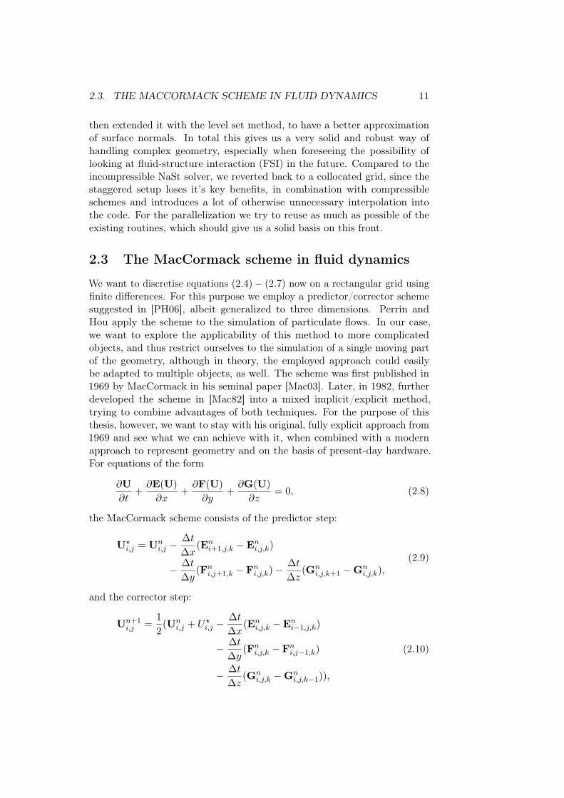
2.3 The MacCormack scheme in fluid dynamics
We want to discretise equations (2.4)− (2.7) now on a rectangular grid usingfinite differences. For this purpose we employ a predictor/corrector schemesuggested in [PH06], albeit generalized to three dimensions. Perrin andHou apply the scheme to the simulation of particulate flows. In our case,we want to explore the applicability of this method to more complicatedobjects, and thus restrict ourselves to the simulation of a single moving partof the geometry, although in theory, the employed approach could easilybe adapted to multiple objects, as well. The scheme was first published in1969 by MacCormack in his seminal paper [Mac03]. Later, in 1982, furtherdeveloped the scheme in [Mac82] into a mixed implicit/explicit method,trying to combine advantages of both techniques. For the purpose of thisthesis, however, we want to stay with his original, fully explicit approach from1969 and see what we can achieve with it, when combined with a modernapproach to represent geometry and on the basis of present-day hardware.For equations of the form
∂U
∂t+∂E(U)
∂x+∂F(U)
∂y+∂G(U)
∂z= 0, (2.8)
the MacCormack scheme consists of the predictor step:
U?i,j = Un
i,j −∆t
∆x(Eni+1,j,k −Eni,j,k)
− ∆t
∆y(Fni,j+1,k − Fni,j,k)−
∆t
∆z(Gn
i,j,k+1 −Gni,j,k),
(2.9)
and the corrector step:
Un+1i,j =
1
2(Un
i,j + U?i,j −∆t
∆x(Eni,j,k −Eni−1,j,k)
− ∆t
∆y(Fni,j,k − Fni,j−1,k)
− ∆t
∆z(Gn
i,j,k −Gni,j,k−1)),
(2.10)

12 CHAPTER 2. AN EXPLICIT COMPRESSIBLE FLOW SOLVER
where U = (ρ, ρu, ρv, ρw) in our case. This method is fully explicit, nosystem of equations needs to be solved. Note that we used forward differencesthroughout the predicting step and backward differences in the correctorphase. In principal this scheme is accurate up to second-order in both timeand space. Applying this to our equations and inserting the equation of state,we deduce the following update rule:
(ρ)?i,j,k = (ρ)ni,j,k − c1∂+i (ρu))ni,j,k − c2∂
+j (ρv))ni,j,k − c3∂
+k (ρw))ni,j,k (2.11)
(ρu)?i,j,k = (ρu)ni,j,k − c1∂+i (ρu2 + c2ρ)ni,j,k − c2∂
+j (ρvu)ni,j,k
− c3∂+k (ρwu)ni,j,k + (2µ+ λ)c4∂
+i ∂−i (u)ni,j,k
+ µc5∂+j ∂−j (u)ni,j,k + µc6∂
+k ∂−k (u)ni,j,k
+ (µ+ λ)c7(∂oi (∂oj vni,j,k)
+ (µ+ λ)c8(∂oi (∂okwni,j,k),
(2.12)
(ρv)?i,j,k = (ρv)ni,j,k − c1∂+i (ρuv)ni,j,k − c2∂
+j (ρv2 + c2ρ)ni,j,k
− c3∂+k (ρwv)ni,j,k + µc4∂
+i ∂−i (v)ni,j,k
+ (2µ+ λ)c5∂+j ∂−j (v)ni,j,k + µc6∂
+k ∂−k (v)ni,j,k
+ (µ+ λ)c7(∂oj (∂oi uni,j,k)
+ (µ+ λ)c9(∂oj (∂okwni,j,k),
(2.13)
(ρw)?i,j,k = (ρw)ni,j,k − c1∂+i (ρuw)ni,j,k − c2∂
+j (ρvw)ni,j,k
− c3∂+k (ρw2 + c2ρ)ni,j,k + µc4∂
+i ∂−i (w)ni,j,k
+ µc5∂+j ∂−j (w)ni,j,k + (2µ+ λ)c6∂
+k ∂−k (w)ni,j,k
+ (µ+ λ)c8(∂ok(∂oi uni,j,k)
+ (µ+ λ)c9(∂ok(∂oj vni,j,k)
(2.14)
and for the corrector step we get
2(ρ)n+1i,j,k = (ρ)ni,j,k + (ρ)?i,j,k − c1∂
−i (ρu))?i,j,k
− c2∂−j (ρv))?i,j,k − c3∂
−k (ρw))?i,j,k
(2.15)
2(ρu)n+1i,j,k = (ρu)ni,j,k + (ρu)?i,j,k − c1∂
−i (ρu2 + c2ρ)?i,j,k − c2∂
−j (ρvu)?i,j,k
− c3∂−k (ρwu)?i,j,k + (2µ+ λ)c4∂
+i ∂−i (u)?i,j,k
+ µc5∂+j ∂−j (u)?i,j,k + µc6∂
+k ∂−k (u)?i,j,k
+ (µ+ λ)c7(∂oi (∂oj v?i,j,k)
+ (µ+ λ)c8(∂oi (∂okw?i,j,k),
(2.16)
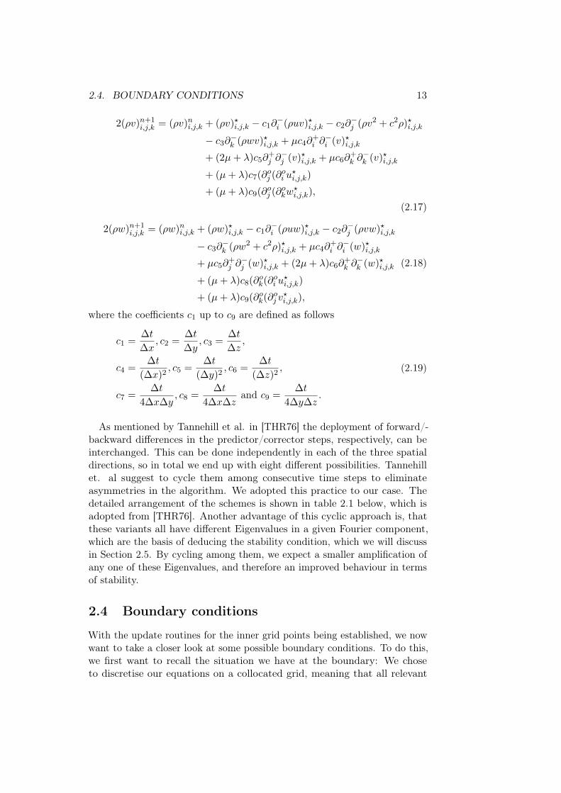
2.4. BOUNDARY CONDITIONS 13
2(ρv)n+1i,j,k = (ρv)ni,j,k + (ρv)?i,j,k − c1∂
−i (ρuv)?i,j,k − c2∂
−j (ρv2 + c2ρ)?i,j,k
− c3∂−k (ρwv)?i,j,k + µc4∂
+i ∂−i (v)?i,j,k
+ (2µ+ λ)c5∂+j ∂−j (v)?i,j,k + µc6∂
+k ∂−k (v)?i,j,k
+ (µ+ λ)c7(∂oj (∂oi u?i,j,k)
+ (µ+ λ)c9(∂oj (∂okw?i,j,k),
(2.17)
2(ρw)n+1i,j,k = (ρw)ni,j,k + (ρw)?i,j,k − c1∂
−i (ρuw)?i,j,k − c2∂
−j (ρvw)?i,j,k
− c3∂−k (ρw2 + c2ρ)?i,j,k + µc4∂
+i ∂−i (w)?i,j,k
+ µc5∂+j ∂−j (w)?i,j,k + (2µ+ λ)c6∂
+k ∂−k (w)?i,j,k
+ (µ+ λ)c8(∂ok(∂oi u?i,j,k)
+ (µ+ λ)c9(∂ok(∂oj v?i,j,k),
(2.18)
where the coefficients c1 up to c9 are defined as follows
c1 =∆t
∆x, c2 =
∆t
∆y, c3 =
∆t
∆z,
c4 =∆t
(∆x)2, c5 =
∆t
(∆y)2, c6 =
∆t
(∆z)2,
c7 =∆t
4∆x∆y, c8 =
∆t
4∆x∆zand c9 =
∆t
4∆y∆z.
(2.19)
As mentioned by Tannehill et al. in [THR76] the deployment of forward/-backward differences in the predictor/corrector steps, respectively, can beinterchanged. This can be done independently in each of the three spatialdirections, so in total we end up with eight different possibilities. Tannehillet. al suggest to cycle them among consecutive time steps to eliminateasymmetries in the algorithm. We adopted this practice to our case. Thedetailed arrangement of the schemes is shown in table 2.1 below, which isadopted from [THR76]. Another advantage of this cyclic approach is, thatthese variants all have different Eigenvalues in a given Fourier component,which are the basis of deducing the stability condition, which we will discussin Section 2.5. By cycling among them, we expect a smaller amplification ofany one of these Eigenvalues, and therefore an improved behaviour in termsof stability.
2.4 Boundary conditions
With the update routines for the inner grid points being established, we nowwant to take a closer look at some possible boundary conditions. To do this,we first want to recall the situation we have at the boundary: We choseto discretise our equations on a collocated grid, meaning that all relevant

14 CHAPTER 2. AN EXPLICIT COMPRESSIBLE FLOW SOLVER
Table 2.1: Applied differencing sequence for the MacCormack scheme; mod-elled on the corresponding table in [THR76]
step pred. ∆x/∆y/∆z corr. ∆x/∆y/∆z
1 F/F/F B/B/B2 B/B/F F/F/B3 F/F/B B/B/F4 B/F/B F/B/F5 F/B/F B/F/B6 B/F/F F/B/B7 F/B/B B/F/F8 B/B/B F/F/F
F forward difference, B backward difference.
quantities (u, v, w, ρ) are located on the same points of a fixed grid. Thephysical boundary will be placed exactly at the location of our boundarypoints, so basically no interpolation between different points is needed.
Velocity boundary conditions
As a result of the choices mentioned above, implementing Dirichlet boundaryconditions is easy, as long as the geometry coincides with the grid. We justset the components of u to the desired values. Most commonly we will have
ui,j,k = vi,j,k = wi,j,k = 0, (2.20)
representing a wall with no-slip conditions located at grid point (i, j, k).
Since in the case of a curved object, our real geometry will deviate fromthese boundary points, we can apply a Taylor expansion to approximate thevelocity usur at the actual boundary point (x, y), which is closest to the givengrid point, if we have access to the outer normal n of the geometry. Usingthe abbrevations ∆x = |x− x| and ∆y = |y − y| we have
usur ≈ ui,j,k + ∆x(ux)i,j,k + ∆y(uy)i,j,k + ∆z(uz)i,j,k. (2.21)

2.4. BOUNDARY CONDITIONS 15
Reorganizing the terms and substituting the appropriate one-sided finitedifferences, i.e.
(ux)ijk =1
2∆x(−ui+2,j,k + 4ui+1,j,k − 3ui,j,k) +O(∆x2),
(uy)ijk =1
2∆y(−ui,j+2,k + 4ui,j+1,k − 3ui,j,k) +O(∆y2),
(uz)ijk =1
2∆z(−ui,j,k+2 + 4ui,j,k+1 − 3ui,j,k) +O(∆z2),
(2.22)
we get the update rule, exemplary to the first octant of the boundary:
ui,j,k =1
c
[−∆x∆y∆z(−ui+2,j,k + 4ui+1,j,k)
−∆x∆y∆z(−ui,j+2,k + 4ui,j+1,k)
−∆x∆y∆z(−ui,j,k+2 + 4ui,j,k+1) + 2∆x∆y∆z(usur)],
(2.23)
with c = 2∆x∆y∆z − 3 [∆x∆y∆z + ∆x∆y∆z + ∆x∆y∆z].
All other cases work analogously, by switching the appropriate signs andwill only be shown once, here: Let (nx, ny, nz) be the outer normal to ourobstacle and (σx, σy, σz) = (σ(nx), σ(ny), σ(nz)), accordingly, the signum ofit. Denote with ∆s a signed version of the cell dimensions, i.e.
∆sx = σx∆x, ∆sy = σy∆y, ∆sz = σz∆z, (2.24)
then our update rule in the general case can be written as
ui,j,k =1
c
[−∆x∆sy∆sz(−ui+2σx,j,k + 4ui+σx,j,k)
−∆sx∆y∆sz(−ui,j+2σy ,k + 4ui,j+σy ,k)
−∆sx∆sy∆z(−ui,j,k+2σz + 4ui,j,k+σz)
+2∆sx∆sy∆sz(usur)],
(2.25)
with now c = 2∆sx∆sy∆sz − 3 [∆x∆sy∆sz + ∆sx∆y∆sz + ∆sx∆sy∆z].
For the sake of clarity, the general case will be omitted throughout thischapter and we will only look at the special case above. The componentsv and w work exactly the same, by replacing u with the according symboland will be omitted, too, when this is evident. We expect to get a smoothervelocity near the boundary, using this boundary condition in the case ofcurved and/or more complex geometries. For a direct comparison of the twomethods in the 2D case see [PH06].
16 CHAPTER 2. AN EXPLICIT COMPRESSIBLE FLOW SOLVER
Prescribed inflow/outflow with a fixed velocity. Additionally, we alsowant to have the possibility to simulate boundaries, with a prescribed inflowvalue, as well as free inflow/outflow type boundary conditions. These can beimplemented as follows: Inflow is just another variant of the above, wherenow the values are different from zero. An open inflow/outflow condition isrepresented by the equation
∂(ρu)
∂x=∂(ρv)
∂y=∂(ρw)
∂z= 0. (2.26)
Finally we implemented symmetry boundary conditions.
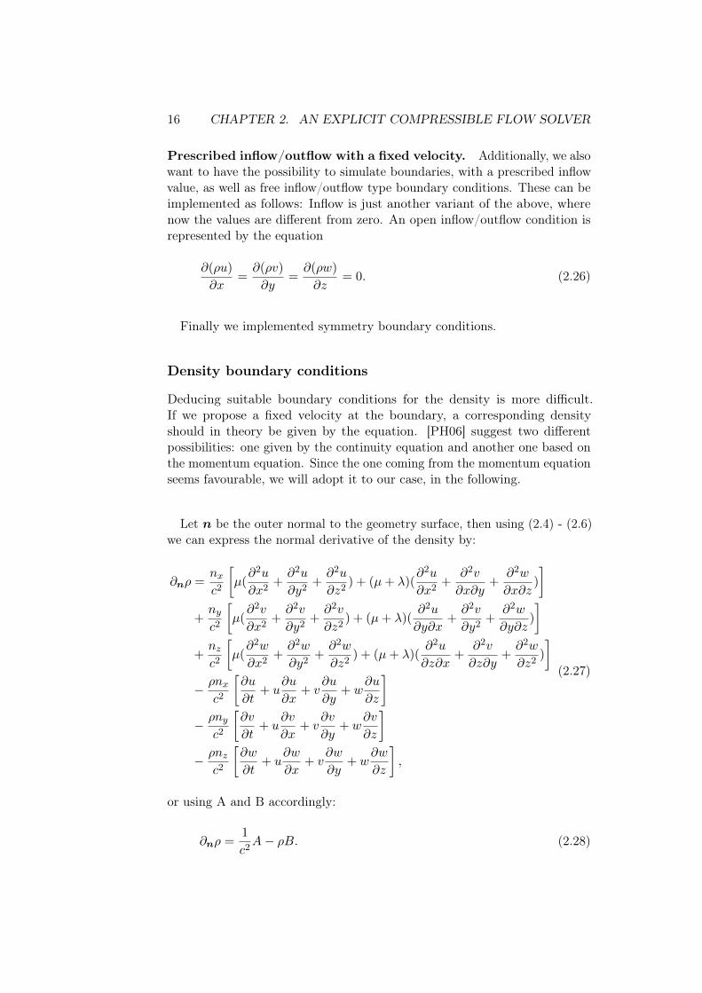
Density boundary conditions
Deducing suitable boundary conditions for the density is more difficult.If we propose a fixed velocity at the boundary, a corresponding densityshould in theory be given by the equation. [PH06] suggest two differentpossibilities: one given by the continuity equation and another one based onthe momentum equation. Since the one coming from the momentum equationseems favourable, we will adopt it to our case, in the following.
Let n be the outer normal to the geometry surface, then using (2.4) - (2.6)we can express the normal derivative of the density by:
∂nρ =nxc2
[µ(∂2u
∂x2+∂2u
∂y2+∂2u
∂z2) + (µ+ λ)(
∂2u
∂x2+
∂2v
∂x∂y+
∂2w
∂x∂z)
]+nyc2
[µ(∂2v
∂x2+∂2v
∂y2+∂2v
∂z2) + (µ+ λ)(
∂2u
∂y∂x+∂2v
∂y2+
∂2w
∂y∂z)
]+nzc2
[µ(∂2w
∂x2+∂2w
∂y2+∂2w
∂z2) + (µ+ λ)(
∂2u
∂z∂x+
∂2v
∂z∂y+∂2w
∂z2)
]− ρnx
c2
[∂u
∂t+ u
∂u
∂x+ v
∂u
∂y+ w
∂u
∂z
]− ρny
c2
[∂v
∂t+ u
∂v
∂x+ v
∂v
∂y+ w
∂v
∂z
]− ρnz
c2
[∂w
∂t+ u
∂w
∂x+ v
∂w
∂y+ w
∂w
∂z
],
(2.27)
or using A and B accordingly:
∂nρ =1
c2A− ρB. (2.28)

2.5. STABILITY 17
Using one-sided second order finite differences, for the normal derivative, weobtain in the first octant:
nx2∆x
(−ρi+2,j,k + 4ρi+1,j,k − 3ρi,j,k)
+ny
2∆y(−ρi,j+2,k + 4ρi,j+1,k − 3ρi,j,k)
+nz
2∆z(−ρi,j,k+2 + 4ρi,j,k+1 − 3ρi,j,k) + ρi,j,kBi,j,k =
1
c2Ai,j,k
(2.29)
If we rearrange this, to solve for ρ we have our desired update rule for ρ:
ρi,j,k =2∆x∆y∆z
c2divAi,j,k −
nx∆y∆z
div(−ρi+2,j,k + 4ρi+1,j,k)
− ny∆x∆z
div(−ρi,j+2,k + 4ρi,j+1,k)
− nz∆x∆y
div(−ρi,j,k+2 + 4ρi,j,k+1).
(2.30)
with div = −3nx∆y∆z − 3ny∆x∆z − 3nz∆x∆y + 2∆x∆y∆zBi,j,k. Thequantities A and B can be calculated beforehand, since the inner fluid pointshave already been updated.
Evidently, this also imposes some restrictions on the feasible geometry:We need to ensure that every fluid domain is at least three cells wide, andno obstacle cells, with fluid on opposite sides, exist. In practice, we canachieve this by refining the underlying grid, but due the cubic scaling of thecorresponding number of cells and the grids uniform nature, this can increasecomputing time by a critical margin.
2.5 Stability
As usual with explicit methods, there is some sort of mandatory Courant-Friedrichs-Levy condition (CFL), that needs to be fulfilled to get any formof stability for our scheme. In the compressible setting, it is important toremember the fact, that we not only need to look at the flow speeds itself, butalso have to consider the speed of sound, which is the rate at which pressurewaves propagate through our domain. So the very thing, that allows us touse an explicit method in the first place, i.e. a finite propagation speed, alsosets the limits in how far we can go within a single time step. So despiteour demand to stay below a certain Mach number, we face the problem, thatvery low number makes our code inefficient, due to the faced restriction ontime steps.
Because of the complexity of the underlying equations, we cannot hope toget a rigorous stability requirement in closed-form for our technique, but the

18 CHAPTER 2. AN EXPLICIT COMPRESSIBLE FLOW SOLVER
following semi-empirical criterion given by Tannehill [THR76] seems to berelatively reliable in giving us a good estimate
∆t ≤ τ
1 + 2/Re∆
[|u|∆x
+|v|∆y
+|w|∆z
+ vsound
√1
∆x2+
1
∆y2+
1
∆z2
]−1
,
(2.31)
where Re∆ = min(ρ|u|∆x/µ, ρ|v|∆y/µ, ρ|w|∆z/µ) and τ ≈ 0.8 is a safetyfactor. This criterion gives us a local restriction for each cell, so we haveto minimize this quantity over our mesh, subsequently, to get a globallyadmissible time step.
The term on the right-hand side
(∆t)CFL ≤[|u|∆x
+|v|∆y
+|w|∆z
+ vsound
√1
∆x2+
1
∆y2+
1
∆z2
]−1
, (2.32)
was identified by MacCormack (see [Mac71]) as the inviscid CFL condition. Heobtained this criterium, by studying the amplification of Fourier componentsof the linearised equation.For a cubic grid and M small enough this reduces to the well-known, muchsimpler condition
∆t ≤ 1
2
∆x
vsound. (2.33)
Remember though, that these can be necessary conditions, at best, which aremostly derived from linearised equations and don’t take difficult boundaryregions into account. Hence, in practice, finding a suitable time step stillcomes with some difficulties and we will see, that either way, this imposessome restrictions on the problems we can solve. We will discuss this later indetail for some of the examples in Chapter 5.
2.6 Parallelization
Even with the most modern CPUs, clocking in the multiple GHz region,tackling interesting fluid problems is only possible, if we employ many ofthem at the same time. In our case, we want to use a big cluster of CPUs lateron. In order to do this, it is necessary to split our problem up and give eachprocessor a piece of the computation, that can, for the most part, be solvedindependently. As most CFD codes, we arrange this, by dividing our domainspatially into chunks of roughly the same computational complexity and thenassigning each of these sub-domains to its own processor. In this process,a big advantage of having a rectangular grid comes into play: Dividingthe computational cost evenly among the processors is easy, since the grid

2.7. AN OVERVIEW OF THE FULL ALGORITHM 19
points of our mesh are distributed evenly among our domain, so we canassume that dividing our domain spatially into blocks of the same size isalso computationally efficient. Since cubes posses the best ratio of volume tosurface, depending on the shape of our domain we try to avoid large aspectratios in our sub-domains. In this manner, the boundaries between adjacentprocessors are split into six distinct directions and communication betweenthe processors can be handled relatively easy: Our update scheme requiresthe values of fluid variables on neighbouring points. If we are close to theborder of our sub-domain, these points might belong to another processorand must therefore be communicated in some way, since each processor isfitted with its own chunk of memory. Even on shared memory machines,arrangements have to be made, in order to prevent simultaneous access tothe same memory blocks. In practice, we exchange these border values aftereach time step and store them in so-called ghost cells, that surround ouractual domain and serve just this purpose of having a local copy of the valueson neighbouring cells. This way we can handle all interfacing between theprocessors in one go, and afterwards, each processor can run the updatescheme for its own variables independently of the rest.
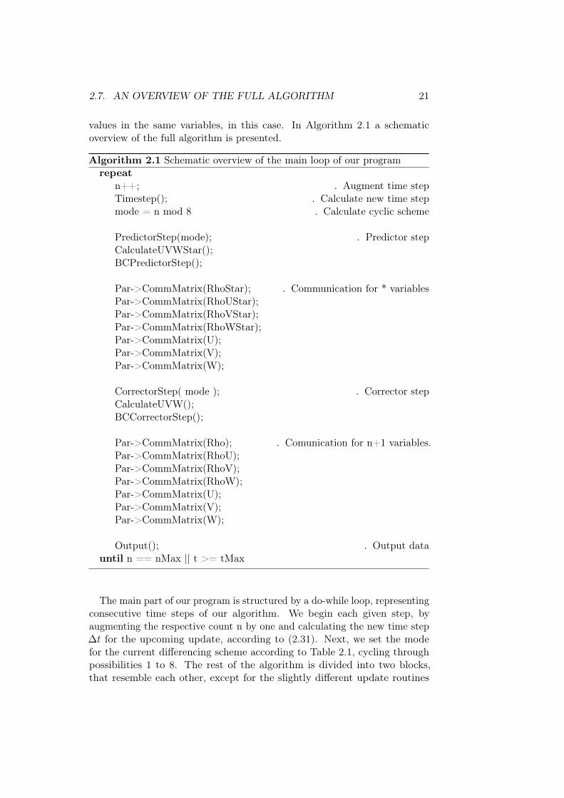
In the actual code, this communication is handled with the Message PassingInterface (MPI). For the present work, we rely on parallelization routinesalready existing in the NaSt3DGP fluid solver. For further details on theexact routines, we refer to [GDN98]. If we take a look back at our updatescheme, we notice that we used up to three cell neighbours in a given directionin our density boundary condition, so we will also need a minimum of threelayers of ghost cells to lose no information. Additionally, at some point, weaccess one neighbouring point in diagonal directions, so we have to take care,that one layer of corner ghost cells is exchanged, as well. Figure 2.1 showsa schematic overview of the required communication in 2D. Despite thisseeming bulk of information that needs to be transferred between processors,we expect a pretty decent efficiency in our parallelization. The results ofsome practical measurements on this question can be found in Section 5.1.
2.7 An overview of the full algorithm
In this section, we want to give a short overview of the implemented algorithm.Again, the algorithm proceeds in a totally linear update routine, in the courseof which no system of equations has to be solved. For the momentum variables,as well as the density, we need two separate fields for the full time step and thepredicted values, respectively, since the information of either values is neededto update the other. In this context, all variables representing predictedvalues, will be indicated by a ∗. Since we don’t use the velocity componentsfor updating the inner grid cells, we can store both predicted and corrected

20 CHAPTER 2. AN EXPLICIT COMPRESSIBLE FLOW SOLVER
I III
II IV
Figure 2.1: Schematic overview of the required communication between fourneighbouring processors in 2D, using tree layers of ghost cells and one cornercell
2.7. AN OVERVIEW OF THE FULL ALGORITHM 21
values in the same variables, in this case. In Algorithm 2.1 a schematicoverview of the full algorithm is presented.
Algorithm 2.1 Schematic overview of the main loop of our programrepeat
n++; . Augment time stepTimestep(); . Calculate new time stepmode = n mod 8 . Calculate cyclic scheme
PredictorStep(mode); . Predictor stepCalculateUVWStar();BCPredictorStep();
Par->CommMatrix(RhoStar); . Communication for * variablesPar->CommMatrix(RhoUStar);Par->CommMatrix(RhoVStar);Par->CommMatrix(RhoWStar);Par->CommMatrix(U);Par->CommMatrix(V);Par->CommMatrix(W);
CorrectorStep( mode ); . Corrector stepCalculateUVW();BCCorrectorStep();
Par->CommMatrix(Rho); . Comunication for n+1 variables.Par->CommMatrix(RhoU);Par->CommMatrix(RhoV);Par->CommMatrix(RhoW);Par->CommMatrix(U);Par->CommMatrix(V);Par->CommMatrix(W);
Output(); . Output datauntil n == nMax || t >= tMax
The main part of our program is structured by a do-while loop, representingconsecutive time steps of our algorithm. We begin each given step, byaugmenting the respective count n by one and calculating the new time step∆t for the upcoming update, according to (2.31). Next, we set the modefor the current differencing scheme according to Table 2.1, cycling throughpossibilities 1 to 8. The rest of the algorithm is divided into two blocks,that resemble each other, except for the slightly different update routines

22 CHAPTER 2. AN EXPLICIT COMPRESSIBLE FLOW SOLVER
discussed in Section 2.3: First we update the inner fluid points in the mainpredictor/corrector step, subsequently, we calculate our velocities by a simpledivision. Finally, we use the gathered information, to provide boundary valuesfor the next iteration and communicate the needed values to the neighbouringghost cells. At the end of each time step we output our data, if so desired.Since the existing NaSt3DGP output routines are designed for the staggeredgrid setup, we adopted our own version of them, giving us straight outputs ofour fluid variables in appropriate VTK (Visualization Toolkit) file formats.

Chapter 3
Geometry representation
What we have seen thus far, is basically a full solver of the compressibleNavier-Stokes equations in a channel, with different boundary conditions forthe walls, the only restriction being the demand of staying in the low Machnumber regime. But besides being able to solve some simple benchmarks, wewant to have a method to represent more complex geometries, that allow us totackle more interesting problems, that are related to real-world applications.In order to do this, some different methods can be considered. A simpleflag-field is easy to implement, but also lacks the kind of flexibility, we seek inthe long run. Another problem with this approach is the bad approximationof the surface normal of our geometry. Another approach is the so-calledlevel set method (LSM) which we want to explore in the upcoming section ofthis work.
3.1 The level set method
The level set method was first outlined by Osher and Sethian in their 1988paper [OS88]. It is a so-called front tracking method, that very generallyallows one to capture the interface between two distinct regions of a domain.Today it is used in many areas such as image processing, computer graphicsor, likewise, computational fluid dynamics (for a more extensive overview seefor example [OF03]). The basic idea is to have a function ϕ, which is definedon the higher dimensional surrounding space, that encodes the movement ofthe evolving surface. What seems at first to be a not very effective way ofdealing with the involved information, turns out to give a very high versatility,when it comes to topological changes of the geometry. In contrast to someother methods, the surface never has to be parametrized and is only modifiedimplicitly, by adjusting the function ϕ. Things like an object splitting apartor the merging of objects, are handled naturally by this framework, whichmakes it very robust. Let us see how this works in a bit more detail.
23

24 CHAPTER 3. GEOMETRY REPRESENTATION
We keep our notation close to Losasso, Fedkiw and Osher ([LFO06]), whogive a neat introduction to level set methods. If we call the enclosed region ofspace Ω− and the interface between Ω− and it’s complement Γ, we demandour level set function ϕ to be a Lipschitz continuos function with the followingcharacterizing properties:
ϕ(x, t) ≤ 0 for x ∈ Ω− (3.1)
ϕ(x, t) > 0 for x /∈ Ω− (3.2)
Then clearly, we have
Γ(t) = x|ϕ(x, t) = 0. (3.3)
We can now implement an evolution of this interface, by a very generalvelocity field a(x, t), that transports the interface. We call this field a todistinguish it from the velocity u, of our flow, since the two need not coincide,here. For this purpose, the velocity needs only to be given in a neighbourhoodof the interface. The equation that describes the advection of the level set isthen given by
∂tϕ+ a · ∇ϕ = 0. (3.4)
It was already introduced in the initial paper by Osher and Sethian ([OS88])and is just called the level set equation. So far, we still have a lot of freedom ofextending ϕ ouside the zero level set. Since, for numerical accuracy, we wantthe function to be as smooth as possible, we prefer it to be a signed distancefunction, at least in a certain band around the interface. Unfortunately thisproperty is not preserved by the solutions to the above transport equation.While small deviations don’t cause much harm, over time we need a methodto restore this property, given our current state of the interface. There aresome different algorithms around to achieve this reinitialization, the detailsof which we don’t want to mention here (see for example [OF01]).
One of the key benefits of the technique, which we want to exploit especially,is the very natural and yet very accurate access to geometric information likethe normal and curvature of our geometry. The normal to our interface Γ issimply given by
n(x, t) =∇ϕ(x, t)
|∇ϕ(x, t)|, (3.5)
whereas the mean curvature κ can subsequently be determined as the diver-gence of the former
κ(x, t) = ∇ ·(∇ϕ(x, t)
|∇ϕ(x, t)|
). (3.6)
3.2. GEOMETRY IMPORT VIA THE STL FILE FORMAT 25
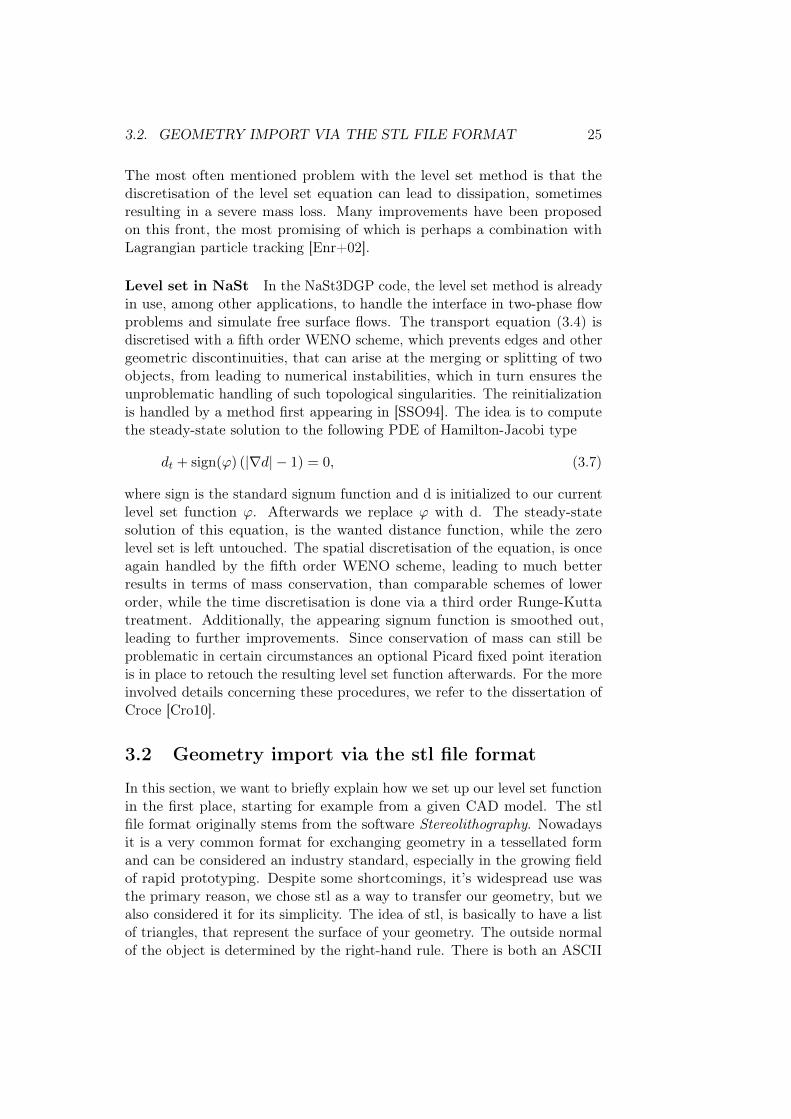
The most often mentioned problem with the level set method is that thediscretisation of the level set equation can lead to dissipation, sometimesresulting in a severe mass loss. Many improvements have been proposedon this front, the most promising of which is perhaps a combination withLagrangian particle tracking [Enr+02].
Level set in NaSt In the NaSt3DGP code, the level set method is alreadyin use, among other applications, to handle the interface in two-phase flowproblems and simulate free surface flows. The transport equation (3.4) isdiscretised with a fifth order WENO scheme, which prevents edges and othergeometric discontinuities, that can arise at the merging or splitting of twoobjects, from leading to numerical instabilities, which in turn ensures theunproblematic handling of such topological singularities. The reinitializationis handled by a method first appearing in [SSO94]. The idea is to computethe steady-state solution to the following PDE of Hamilton-Jacobi type
dt + sign(ϕ) (|∇d| − 1) = 0, (3.7)
where sign is the standard signum function and d is initialized to our currentlevel set function ϕ. Afterwards we replace ϕ with d. The steady-statesolution of this equation, is the wanted distance function, while the zerolevel set is left untouched. The spatial discretisation of the equation, is onceagain handled by the fifth order WENO scheme, leading to much betterresults in terms of mass conservation, than comparable schemes of lowerorder, while the time discretisation is done via a third order Runge-Kuttatreatment. Additionally, the appearing signum function is smoothed out,leading to further improvements. Since conservation of mass can still beproblematic in certain circumstances an optional Picard fixed point iterationis in place to retouch the resulting level set function afterwards. For the moreinvolved details concerning these procedures, we refer to the dissertation ofCroce [Cro10].
3.2 Geometry import via the stl file format
In this section, we want to briefly explain how we set up our level set functionin the first place, starting for example from a given CAD model. The stlfile format originally stems from the software Stereolithography. Nowadaysit is a very common format for exchanging geometry in a tessellated formand can be considered an industry standard, especially in the growing fieldof rapid prototyping. Despite some shortcomings, it’s widespread use wasthe primary reason, we chose stl as a way to transfer our geometry, but wealso considered it for its simplicity. The idea of stl, is basically to have a listof triangles, that represent the surface of your geometry. The outside normalof the object is determined by the right-hand rule. There is both an ASCII

26 CHAPTER 3. GEOMETRY REPRESENTATION
and a binary version of the stl file format. Due to the much improved filesizes and even simpler structure, we only considered the binary version forour code.
Constructing the level set function
Once the stl-file is loaded, a point in polygon test is used to implement aroutine IsInside, which decides if a given grid point, is inside the objectspanned by the stl surface or outside. This is done via a so-called ray castingalgorithm. First, a direction is determined, in which an outgoing ray strikes novertex or edge of the triangles, that make up our model. Then, for each of thetriangles, we decide if the ray passes through it. Therefore, we initially check,if it intersects the plane spanned by that triangle, and if so determine if theintersection is inside the triangle. Counting up the number of triangles, thatour ray hits on its way, we get the result: If the number is odd, we are locatedin the region enclosed by the polygon surface, otherwise we are outside. Withthe use of this function, a characteristic function of the geometry is created,and the corresponding flag field can already be put in place. The level setfunction, finally, is created from this characteristic function by applying thereinitialization procedure, described earlier, to it. By this procedure a fulllevel set distance function is generated on the grid, and can be kept untilthe end of the simulation, since at the current stage of our code, we don’tmanipulate the function itself, but only translate and/or rotate it.
3.3 Comparison to the flag-field
To demonstrate the advantage of the level set method over the pure flag-field,we want to exemplarily show the three different stages of an imported modelin our code. The chosen example is the model of a motorcycle helmet attachedto a very simple torso. The original stl file consists of ca. 3.500 triangles andwas modelled with the CAD-software Pro/ENGINEER. It is positioned in acubic block of side length 0.6m, which is discretised with a grid consisting of60 cells in each direction, which corresponds to 216.000 cells in total. Thethree variants, visualized with ParaView, are shown in Figures 3.1 to 3.3,according to their order of appearance during a run of the algorithm. Asone can clearly see, at such a resolution,the general shape of the model isrepresented relatively accurate by the flag-field, but the surface normal beingrestricted to 6 different directions, makes the approximation still look veryclunky. In comparison, the level set contour looks very smooth, one can easilysee the much improved behaviour, regarding normal directions, which weextensively use in our boundary conditions, as well as in the computation offorces on our obstacles, as we will see in the next chapter. The only drawbackbeing, that sharp edges also get smoothed out in the process and have a smallradius applied to them.

3.3. COMPARISON TO THE FLAG-FIELD 27
Figure 3.1: Step 1: Stl model of a motorcycle helmet, left half visualized withedges
Figure 3.2: Step 2: Flag field threshold of a motorcycle helmet, left halfvisualized with edges

28 CHAPTER 3. GEOMETRY REPRESENTATION
Figure 3.3: Step 3: Level set contour of a motorcycle helmet, left halfvisualized with edges
Chapter 4
Simulation of moving objects
Now, that we have static geometries implemented, we want to look at thepossibility of simulating geometries, evolving over time. The easiest class ofsuch problems is clearly a constant object moving through the scene. Wewant to tackle this problem in this section, with the help of the alreadyimplemented level set method. In order to go ahead, we need to make sure,that our boundary conditions still work on a moving boundary.
4.1 Adjusting the boundary conditions
First of all, we assume that all the boundary points on the object are only ofno-slip type. Although a generalization to allow inflow/outflow boundariescould easily be implemented, we don’t want to consider this case here andmost applications don’t require it, anyway. Let us remember the equationfor such no-slip boundaries, again only accounting for the first octant:
ui,j,k =1
c
[−∆x∆y∆z(−ui+2,j,k + 4ui+1,j,k)
−∆x∆y∆z(−ui,j+2,k + 4ui,j+1,k)
−∆x∆y∆z(−ui,j,k+2 + 4ui,j,k+1) + 2∆x∆y∆z(usur)],
(4.1)
with c = 2∆x∆y∆z − 3 [∆x∆y∆z + ∆x∆y∆z + ∆x∆y∆z].
The only thing we need to do now, is to feed the velocity of the objectsmovement (represented by its centre of mass) into this equation as the valuefor usur, vsur or wsur, accordingly. The equation itself works right out of thebox.
29

30 CHAPTER 4. SIMULATION OF MOVING OBJECTS
Velocity prediction for leaking boundary points
Looking closer, there is one other small thing we need to consider, though.Our object will be moved after the boundary values for the corrector step areset, and right before we advance to the next time step, starting with the usualpredictor step. So there usually will be points that were inside the obstaclebefore, and now become the new boundary. Both, velocity and density valuesat these points will be accessed in the following predictor step, when updatingtheir neighbours, that in turn were part of the boundary and now changedto be regular fluid cells. In other words, points "leaking" from the geometryneed to be addressed. We need to find a way to predict a sensible velocity anddensity for them. This will, once again, be done by applying the one-sidedsecond order differences from (2.22) to a taylor expansion. Assuming we arein the first octant, we have
ui,j,k ≈ ui+1,j,k −∆x(ux)i+1,j,k. (4.2)
Inserting our differencing scheme from (2.22), we get
ui,j,k ≈1
2(5ui+1,j,k − 4ui+2,j,k + ui+3,j,k). (4.3)
Since we can do the analogous approximation in directions y and z, we averagethem with the normal n as a weight, to get our final update rule:
ui,j,k =n2x
2(5ui+1,j,k − 4ui+2,j,k + ui+3,j,k)
+n2y
2(5ui,j+1,k − 4ui,j+2,k + ui,j+3,k)
+n2z
2(5ui,j,k+1 − 4ui,j,k+2 + ui,j,k+3)
(4.4)
Exactly the same reasoning can be used for the density, as well. As a finalnote, we remember, that we already use three layers of ghost cells in theparallelization, so no adaptations have to be carried out on this front.
Tracking the boundary
In the last section we have discussed the changes to our boundary conditions,that need to be implemented if we want to simulate moving obstacles. Inour code, boundary points are saved in lists, gathering points of the sameboundary type, which are established on the basis of our flag field. In theend, moving our geometry is realized by moving the level set function, bywhich it is defined. Hence, in order to keep track of our boundary points, we
4.2. MOVING GEOMETRIES WITH A PRESCRIBED VELOCITY 31
need to update our flag field, as well as the corresponding lists, accordingly.In Practice, after each time step, we go through our level set field and checkfor sign changes among neighbouring points. If we detect a changing sign weset the appropriate flag. If a given cell, was marked as an obstacle cell before,and is now on the boundary, we additionally mark it as leaking. This way, wemark it to receive the special care discussed in the last subsection. After thisprocedure, we rebuild our lists and update our leaking points, as described.
4.2 Moving geometries with a prescribed velocity
Fundamentally, we are interested in having both, objects with a prescribedvelocity, as well as geometries driven by the flow. In Chapter 3 we described,how to generally transport a level set function by a general velocity field a.While this setting gives us a very high flexibility, in terms of modifying ourobject, in the course of this thesis, we want to restrict ourselves to the specialcase of globally transporting the level set, i.e. moving our object as a whole,rather than locally moving its boundaries, and therefore possibly altering itsshape, while the latter still remains as a future option. Let uCoM (t) be thevelocity we want to assign to our object, which is represented by its centreof mass (CoM). Then, in the general setting from above, our case can bedescribed as
a(x, t) = uCoM (t). (4.5)
Let s = (sx, sy, sz) bet the distance our obstacle moves in a given time step.Then we evidently have
sx(tn) = uCoM (tn) ∆t
sy(tn) = vCoM (tn) ∆t
sz(tn) = wCoM (tn) ∆t
(4.6)
We use a Semi-Lagrangian ansatz to implement this movement, whichmeans, that we calculate new values at our grid points, by going backwardsin time to deduce their initial position before the movement occurred. Let uslook at the situation for the grid point (i,j,k). Before the translation it waslocated at coordinates x
yz
=
i∆x− sx(tn)j∆y − sy(tn)k∆z − sz(tn)
(4.7)

32 CHAPTER 4. SIMULATION OF MOVING OBJECTS
Figure 4.1: Basic idea of the Semi-Lagrangian ansatz
Let p1 = (i1, j1, k1) and p2 = (i2, j2, k2) be the two unique grid points withcoordinates (x1, y1, z1) and (x2, y2, z2) such that
x1 < x < x2 = x1 + ∆x
y1 < y < y2 = y1 + ∆y
z1 < z < z2 = z1 + ∆z
(4.8)
We interpolate the new value for the level set function L at (i,j,k) betweenthe eight grid points surrounding its original position:
Li,j,k(tn+1) =1
∆x∆y∆z
[(x2 − x)(y2 − y)(z2 − z)Li1,j1,k1(tn)
+(x− x1)(y2 − y)(z2 − z)Li2,j1,k1(tn)
+(x2 − x)(y − y1)(z2 − z)Li1,j2,k1(tn)
+(x− x1)(y − y1)(z2 − z)Li2,j2,k1(tn)
+(x2 − x)(y2 − y)(z − z1)Li1,j1,k2(tn)
+(x− x1)(y2 − y)(z − z1)Li2,j1,k2(tn)
+(x2 − x)(y − y1)(z − z1)Li1,j2,k2(tn)
+(x− x1)(y − y1)(z − z1)Li2,j2,k2(tn)]
(4.9)
Obviously, we need to make sure, that our object moves less than one celllength per time step with this scheme, but this is automatically secured byour stability condition including the speed of sound, since we don’t want tosimulate objects anywhere close to the speed of sound.

4.3. TRANSLATION VS. ROTATION 33
4.3 Translation vs. rotation
Up until this point, we have only talked about translational movement, but inprinciple, the above method could be easily extended to rotational movement,as well. The only thing that needed to be done is to incorporate the rotationinto the Semi-Lagrangian ansatz, where we compute the original position ofour point. There is another problem with this method altogether, though,which we want to explain in this Section, and which finally led to the decision,to only consider translations for the present thesis.
When trying the above method in practice, we soon encountered terribleproblems with the stability of our level set function. Even after very shorttimes, we could see a severe mass loss and some deformations of the object, aswell. Apparently, interpolating the level set function in such a manner doesn’twork very well, if you do it many times over. This effect is especially gravein our case, due to the small time steps mandated by the CFL-condition,resulting in a huge number of successive interpolations. Our first idea toovercome this problem, was to not interpolate successively, for each time step,but to always start from the original level set function, that was generatedby the reinitialization procedure. For this to work, we only have to addup the distances from Equation 4.6 as we go. This way, there’s never morethan one interpolation, since we always start fresh with the original level-setfield. In turn, however, the position of our point of interest and its originallocation, were we interpolate the new value, drift apart, in the same manneras we move our object. This is no problem in a serial environment, whereonly one processor is involved, and consequently has access to the completelevel set field. If we want to run our algorithm in a parallel fashion on manyprocessors, though, we face the issue of only having a local piece of the fieldin the memory of each processor. Both, having to communicate all valueswhere cells of a given processor emerged from, which is a very elaborateand tedious procedure, as well as having a global level set function for eachprocessor of its own, which is blatantly inefficient memory-wise and defeatsthe purpose of the parallelization in the first place, are no practically usefulsolutions to this.
For translations, at least, there is a more elegant solution: We can dothe above, i.e. interpolating from the initial level set function, until ourobject has moved by a whole grid cell in any given direction. When thishappens, we move our original level set, which we use as a source for theinterpolation, by one grid cell in this direction. This process doesn’t requireany interpolation, since the grid is mapped to itself. This way, the origin ofeach grid pont always keeps track with the movement of the obstacle, andtherefore no communication is needed, yet still, there is never more thana single interpolation required to deduce the value for a given position, so

34 CHAPTER 4. SIMULATION OF MOVING OBJECTS
we don’t run into the problems discussed before. The only downside to thismethod is, that there is no obvious generalization to rotations, since there isno natural analogue of moving by one grid cell. The first angle at which arotation of a (quadratic) grid aligns with its initial origin is at 90°, which isway too coarse to help with the problem at hand. Since no other solution wasfound in the time-frame of this work, we restrict ourselves to translationalmovement for the point being, although the rest of the theory could easilybe adapted, to the general case. In the end everything comes down to aparallelization issue, which seems difficult to solve, but there is no pointrunning in serial, whatsoever.
4.4 Bidirectional coupling
In the following Section, we want to see how we can generalize the aboveto allow for bidirectional coupling, too. Again, we restrict ourselves totranslational movements, although the coupling would work exactly the samefor rotations. In some way, this bidirectional coupling has to be based oncomputing the forces our fluid exercises on the obstacle at hand. Once wehave done this, we just feed these forces back into the loop by adjusting ourCentre-of-Mass velocity uCoM via Newton’s law. In the end our problembasically comes down to computing drag/lift forces on a body, as well asits mass or rather its volume. The calculation of both of these quantitiesrelies on integration. Most generally, we can express the force on an obstacleimmersed into our fluid, by integrating the stress among its surface, in otherwords
F =
∫S
σ · ndS, (4.10)
where n is of course the outer normal to the surface S. Now, to be consistentwith the equations presented in Chapter 2, our total stress σ is given by
σ = −p I + µ(∇u+ (∇u)T )− λ(∇ · u) I, (4.11)
where we discretise all appearing derivatives with central differences. Insertingthis above, all that’s left to do, is to approximate the integral in our discretesetting. There are many different ways of doing this for a fixed mesh, someusing very elaborate interpolation techniques. In 2012 Haeri and Shrimptonpublished a review paper on a few of these methods ([HS12]). Here, wewant to keep things a little simpler, though. Again, we make use of thenormal, which is readily provided by our level-set function. To discretise theintegral itself, first, we want to bring it to a slightly different form. SinceS = x|ϕ(x) = 0 and |∇ϕ| = 1, using a change of variables, we can rewrite
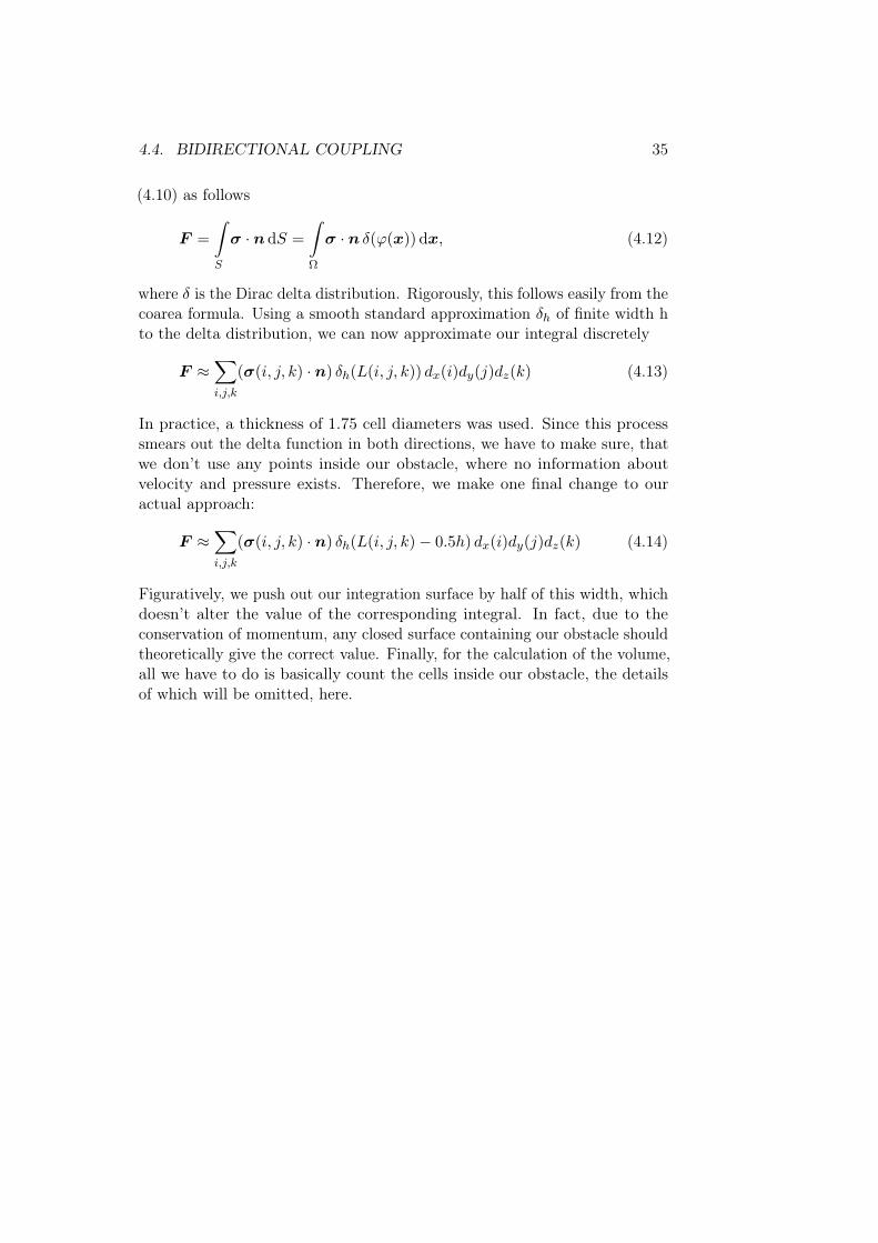
4.4. BIDIRECTIONAL COUPLING 35
(4.10) as follows
F =
∫S
σ · ndS =
∫Ω
σ · n δ(ϕ(x)) dx, (4.12)
where δ is the Dirac delta distribution. Rigorously, this follows easily from thecoarea formula. Using a smooth standard approximation δh of finite width hto the delta distribution, we can now approximate our integral discretely
F ≈∑i,j,k
(σ(i, j, k) · n) δh(L(i, j, k)) dx(i)dy(j)dz(k) (4.13)
In practice, a thickness of 1.75 cell diameters was used. Since this processsmears out the delta function in both directions, we have to make sure, thatwe don’t use any points inside our obstacle, where no information aboutvelocity and pressure exists. Therefore, we make one final change to ouractual approach:
F ≈∑i,j,k
(σ(i, j, k) · n) δh(L(i, j, k)− 0.5h) dx(i)dy(j)dz(k) (4.14)
Figuratively, we push out our integration surface by half of this width, whichdoesn’t alter the value of the corresponding integral. In fact, due to theconservation of momentum, any closed surface containing our obstacle shouldtheoretically give the correct value. Finally, for the calculation of the volume,all we have to do is basically count the cells inside our obstacle, the detailsof which will be omitted, here.

36 CHAPTER 4. SIMULATION OF MOVING OBJECTS

Chapter 5
Example results
In this chapter we want to show a selection of results, we could achieve onthe basis of the previously presented theory. Each computation is performedto show a specific feature of the code and is only exemplary. A multitude ofdifferent possibilities exist beyond the presented scenarios. In general, thechapter is divided roughly into two areas: The first two sections are devotedto validate our code in different ways. Subsequently, we want to explore thepossibilities that can be realized with the algorithms at hand, showing somenice examples, in the progress. All visualizations throughout the chapter havebeen carried out using ParaView and the Visualization Toolkit (VTK). Thelabel vectors Magnitude in the corresponding figures refers to the magnitudeof the velocity field u, always expressed in m/s. Allthough our theory, aswell as our code is formulated to operate with density, rather than pressure,for the output and analysis of the flow, we decided to opt for a zero-centredpressure, which is simply given by
p = v2sound(ρ− ρ0), (5.1)
where ρ0 is the resting density of the fluid. The two convey the sameinformation, yet the visualization in terms of pressure is easier to present andmore familiar, coming from the incompressible case. All appearing plots weredone with the aid of Gnuplot.
5.1 First Tests
Having implemented the preceding methods, we want to test them withsome simple cases, as a preliminary point, before going over to more complexproblems. Therefore, in this section, we try to replicate some standard drivencavity results, look at the progression of L2 errors on different grid resolutionsand finally examine the parallel scaling of our code on a CPU cluster, to getan idea how it performs in the most general setting.
37

38 CHAPTER 5. EXAMPLE RESULTS
Driven cavity
As a first test, we try to replicate the results from Perrin and Hou ([PH06])for a driven cavity scenario in 2D. To recreate their setting, we use thesymmetric boundary conditions presented in Section 2.4 to create a pseudo2D form of the algorithm. Physically, the two experiments are equivalent,but a confirmation of the results still gives us a first hint at the correctnessof our code, as well as the underlying equations.
Figure 5.1: Velocity field of a driven cavity on a 256x256 grid at Re = 100(left) and Re = 400 (right) and U = 1m/s; stopped after simulated time of24 s. The purple crosses mark the vortex centres found by [Hou+95].
The calculations are performed on a uniform grid of 256x256 cells, represent-ing the domain Ω = [0, 1]× [0, 1], and 32 cells in the (symmetric) z-direction.The flow is driven by the upper border of the domain moving at a speed of1m/s to the right. No-slip conditions are enforced on all other walls of thecavity. To remain in the nearly incompressible region the speed of sound isset to 10m/s, resulting in a Mach number M = 0.1. The experiment is thenconducted at a Reynolds number of 100 and 400, each, and run until steadystate is reached.The resulting velocity fields and corresponding streamlinesare shown in Figure 5.1. In both cases a large primary eddy vortex can befound spanning most of the cavity, withsome smaller vortices emerging in thebottom corners of the domain. In accordance with our expectations, in the

5.1. FIRST TESTS 39
course of the higher Reynolds number, the primary vortex moves closer tothe middle of the cavity and the secondary vortices become more distinct,due to the lower viscosity. The centres of the primary vortices are in goodaccordance with the results found by Ghia et al. ([GGS82]) and Hou etal. ([Hou+95]), who give coordinates of (0.6196, 0.7373) at Re = 100 and(0.5608, 0.6078) at Re = 400 using a Lattice-Boltzmann method. Eventually,with higher Reynolds numbers, the vortices will become unstable as reportedby Ghia et al. All in all we can securely replicate the results found in theliterature and at first glance computing times seem to be competitive, aswell.
Progression of L2-Errors
Next, we want to perform further tests on the accuracy of our solutions,especially when increasing grid resolutions. Due to the lack of exact solutionsfor the compressible Navier-Stokes equations, showing any form of convergenceproves very difficult. What we can do instead, to estimate convergence order,is to compute a solution on a very fine mesh and examine the behaviour ofthe algorithm when approximating it with coarser variants from below. Wewant to use the experiment above, and calculate the L2 error for differentresolutions compared to a reference grid of 800x800 cells. Grid sizes of therelated coarse meshes varied from 25x25 cells up to 400x400 cells, with atwo-fold margin left over to our reference solution, in order for the assumednegligible error on the fine grid not to distort the picture. To capture possibletime-dependant effects, the simulation wasn’t run until steady-state, butwas stopped after a fixed time of 4.0 s. Throughout the study, the Reynoldsnumber was set to 100. For the comparison, the result on the coarser gridwas then interpolated to the finer reference grid, and an approximation tothe L2 norm was calculated in the following way:
‖U‖L2 =
∫Ω
|U(x, y, z)|2 dL3(x, y, z)
1/2
≈
∑i,j,k
|U(i, j, k)|2dx(i)dy(j)dz(k)
1/2(5.2)
Having established the norm, the absolute error ε and relative error η arethen defined as follows:
εU,L2 = ‖Ufine − Ucoarse‖L2 (5.3)
ηU,L2 =‖Ufine − Ucoarse‖L2
‖Ufine‖L2
(5.4)

40 CHAPTER 5. EXAMPLE RESULTS
In practice, the filters ResampleWithDataset, IntegrateVariables and Calcu-lator, provided by the ParaView Software, were used to perform the requiredcomputations. In the same manner we can calculate the related errors forthe pressure. The results of the study are listed in Table 5.1 alongside alogarithmic plot, comparing the data with an appropriate fit in Figure 5.2,to estimate the order of convergence. In conclusion, the results are prettyencouraging: The order of convergence, for both the velocity and the pressureincreases, the higher our resolution goes. In general, the behaviour for thevelocity, going from 1.53 in the beginning, to a value of 2.33 in the final step,seems to be slightly better than for the pressure. The last two values, evengoing above the proposed second order, are probably due to the fact, that ourassumption of a negligible error on the reference grid, becomes less accurate,the closer we get to it. Therefore, especially the last entry, for a resolutionof 400 points, is probably overshooting the actual value. The correspondingfit, which estimates an order of 1.79 for the velocity and around 1.46 for thepressure, should give us a more accurate picture of our study. Still, the resultis only slightly below the theoretically proposed second order convergence,and therefore very gratifying, indeed.
Table 5.1: Relative L2 errors for different resolutions compared to a 800x800reference grid
grid size ηU,L2 orderU ηp,L2 orderp
25× 25 9.73e-02 - 1.42e+00 -50× 50 3.36e-02 1.53 5.72e-01 1.31
100× 100 1.09e-02 1.62 2.26e-01 1.34200× 200 2.98e-03 1.88 8.30e-02 1.45300× 300 1.30e-03 2.03 4.20e-02 1.68400× 400 6.67e-04 2.33 2.36e-02 2.00
Strong scaling
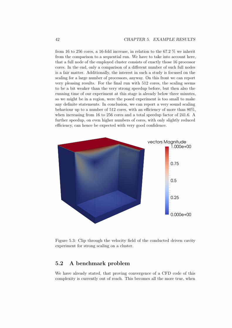
Since the parallelization of CFD codes is indispensable in order to tackleinteresting problems, we want to take a look at the performance of our codeon a big CPU cluster, next. We want to see what kind of efficiency we canexpect with our code in this regard. The subsequent study was performedon a parallel CPU cluster of the University of Bonn. In total, the deployedcluster Atacama consists of 1248 Intel Xeon CPU E5-2560 2.60 GHz cores,supplied by 78 PowerEdge M620 compute nodes. Each of these nodes comeswith 16 CPU cores. The system is equipped with 4992 GB of memory, in

5.1. FIRST TESTS 41
0.0001
0.001
0.01
0.1
1
10 100 1000No. of grid points
ηU,L2
ηp,L2
c/x1.79
c/x1.46
Figure 5.2: Progression of L2 errors for the velocity U and the pressure pcompared to the respective convergence order on a logarithmic scale
total, and the MPI communication routines are conducted by 56 GB/secInfiniband connections. The cluster is operated by the Institute for NumericalSimulation and the Sonderforschungsbereich 1060 at University of Bonn anddisplays a Linpack performance of 20630 GFlop/s at a parallel efficiency of80%.
For the following comparison, running times of the complete programexecution were measured. To avoid static costs distorting the picture forhigher numbers of processors, data outputs were disabled and the problemwas chosen to be reasonably solvable for the total range of a single core upto the maximum of 512 cores we used. The conducted calculation is a nowfully three dimensional driven cavity on a cubic grid with 256 cells in eachdirection, which amounts to ca. 16.8 Mio. cells in total. The simulation wasrun until a fixed time of 0.5s was reached. A clip through the correspondingvelocity field is shown in Figure 5.1. The results of our study, concerningspeedup, as well as the corresponding efficiency, can be seen in Table 5.2 andFigure 5.4. At a first glance, the observed efficiency is distinctly above 50 %up to a number of 256 cores and is thus already very reasonable. Lookingmore closely, especially the scaling above a number of 16 cores seems to bevery good. Indeed, we can attest an efficiency of 80.2 %, when increasing
42 CHAPTER 5. EXAMPLE RESULTS
from 16 to 256 cores, a 16-fold increase, in relation to the 67.2 % we inheritfrom the comparison to a sequential run. We have to take into account here,that a full node of the employed cluster consists of exactly those 16 processorcores. In the end, only a comparison of a different number of such full nodesis a fair matter. Additionally, the interest in such a study is focused on thescaling for a large number of processors, anyway. On this front we can reportvery pleasing results. For the final run with 512 cores, the scaling seemsto be a bit weaker than the very strong speedup before, but then also therunning time of our experiment at this stage is already below three minutes,so we might be in a region, were the posed experiment is too small to makeany definite statements. In conclusion, we can report a very sound scalingbehaviour up to a number of 512 cores, with an efficiency of more than 80%,when increasing from 16 to 256 cores and a total speedup factor of 241.6. Afurther speedup, on even higher numbers of cores, with only slightly reducedefficiency, can hence be expected with very good confidence.
Figure 5.3: Clip through the velocity field of the conducted driven cavityexperiment for strong scaling on a cluster.
5.2 A benchmark problem
We have already stated, that proving convergence of a CFD code of thiscomplexity is currently out of reach. This becomes all the more true, when

5.2. A BENCHMARK PROBLEM 43
1
2
4
8
16
32
64
128
256
1 2 4 8 16 32 64 128 256 512
Speedu
p
No. of cores
0
0.2
0.4
0.6
0.8
1
1 2 4 8 16 32 64 128 256 512
Efficiency
No. of cores
Figure 5.4: Speedup (top) and efficiency (bottom) plot for up to 512 coreson a CPU-cluster

44 CHAPTER 5. EXAMPLE RESULTS
Table 5.2: Speedup and efficiency of a three dimensional driven cavity simu-lation on up to 512 cores
no. of cores absolute time [s] speedup efficiency
1 40981 1.0 100.0 %4 11778 3.5 87.0 %8 6273 6.5 81.7 %16 3811 10.8 67.2 %32 1977 20.7 64.8 %64 1073 38.2 59.7 %128 556 73.8 57.6 %256 297 138.2 54.0 %512 170 241.6 47.2 %
we consider more complicated experiments, like the external flow aroundan obstacle. Comparing the results of our algorithm to exact solutions isdifficult, as well. Although some analytic solutions can be found in theliterature (see i.e. [Whi91]), they are mostly restricted to the one dimensionalcase or don’t solve the full Navier-Stokes equations, but some simplifiedversion. Another approach for the verification of CFD codes is the Methodof manufactured solutions (MMS) [OT02] which aims at manufacturingexperiments specifically, such that a given solution emerges. The AIAA CodeVerification Project [Ghi+10] lists examples of this method, but none of themseems applicable to our special situation. Yet, there are some tightly definedbenchmark cases around, which allow the direct comparison to solutions ofother CFD codes or physical experiments, that are conducted in wind orwater channels. We want to see, if we can find something that suits oursituation. Most compressible forms, like [LL87], focus on shock waves orother high Mach number phenomena, which are not in our interest or reach.What stays as an option, is to see if we can replicate results of incompressiblebenchmarks, if we resort to a small enough Mach number, by adjusting thespeed of sound accordingly. This is what we want to try in the upcomingsection.
Cylinder benchmark by Turek and Schäfer
We try to adopt a benchmark proposed by Turek and Schäfer for incom-pressible CFD codes. The test was first established in 1996 in [TS96], butthe most recent results were published in [BMT12] in 2012. The proposed

5.2. A BENCHMARK PROBLEM 45
task is to examine the flow around a cylinder of diameter D, positioned in aprescribed channel, at a Reynolds number of Re = UD/ν = 20, where U is acharacteristic velocity of the flow. As a means of evaluation, drag and liftforces, exerted on the body, ought to be calculated. A display of the exactsetting, including the dimensions of the channel, as well as the position ofthe cylinder is given in Figure 5.5, which is adopted from Turek and Schäfer.
Figure 5.5: Setup and main dimensions of the 3D-1Z cylinder benchmarkwith circular cross-section according to Turek and Schäfer; taken from [TS96]
In the benchmark, a parabolic inflow profile according to the followingequation is specified on the inflow plane:
u(0, y, z) = 16Umyz(H − y)(H − z)/H4,
v(0, y, z) = w(0, y, z) = 0,(5.5)
where H = 0.41m and Um = 0.45m/s denotes the maximal inflow velocityat the center of the channel. The characteristic velocity U is then
U =4
9u(0, H/2, H/2) = 0.2m/s, (5.6)
which gives us the desired Reynolds number of 20. On the back of thechannel a free in-/outflow condition is used, and on all other walls standardno-slip conditions are prescribed. Drag and lift forces, denoted by FD andFL, accordingly, are defined as follows
FD =
∫S
(µ∂vt∂n
ny − pnx) dS (5.7)
FL = −∫S
(µ∂vt∂n
nx + pny) dS, (5.8)

46 CHAPTER 5. EXAMPLE RESULTS
where n is the outer normal of the cylinder with components nx, ny and nz.Since this is a special case of the components of equation (4.11), except forthe extra term concerning the bulk viscosity, we use the same routines as forthe bidirectional coupling. The corresponding dimensionless coefficients cDand cL, for completion, are then
cD =2FD
ρU2DH(5.9)
cL =2FL
ρU2DH. (5.10)
The integration in the expressions for the lift and drag forces are performedas described in Section 4.4. In addition we calculated the volume of theactual cylinder in our scene, to compare it to the magnitude of our deviationsin lift and drag coefficients.
We performed calculations at different resolutions, as well as differentvalues for the speed of sound. The exact setup is listed in Table 5.3. Sinceboth resolution, as well as a higher speed of sound considerably increasecomputational cost, we cannot have both at an astronomically high level atthe same time, but rather have to take compromises. To see what influenceeach of the parameters have, we tried both variants and want to comparethe results. For all runs, we resorted to standard no-slip conditions on thecylinder, as the boundary condition presented in section 2.4 led to problemswith stability.
Table 5.3: Grid size and speed of sound of the different simulation runs; ×marks performed runs
grid size \ vSound 10 40 80 160
250× 41× 41 × × × ×500× 82× 82 ×
750× 123× 123 ×1.000× 164× 164 ×
Having declared the setup, we can now go forth and perform the calculations.First, we want to look at how good we can even approximate the cylinderwith our current method. Therefore, we calculate the volume enclosed bythe obstacle cells, that make up our cylinder. A comparison of these volumeswith the correct volume of the cylinder is shown in Table 5.4.

5.2. A BENCHMARK PROBLEM 47
Table 5.4: Rel. error of the cylinder volume at different grid resolutions
no. points in x volume rel. error
250 0.002184 32.2 %500 0.002760 14.3 %750 0.002931 9.0 %
1.000 0.003007 6.6 %exact 0.003220 0
Figure 5.6: Approximation of the cylinder outline by the flag field and thelevel set contour at a resolution of 250x41x41 (left) and 500x82x82 (right)

48 CHAPTER 5. EXAMPLE RESULTS
We can see, that the error is quite big at the beginning at over 30 %. Even fora very fine resolution of 1.000 grid cells in the flow direction, which amountsto nearly 27 Mio. cells in total, we have an error in the representation of thevolume, which is not negligible at 6.6 %. We want to see, if we can improvethis behaviour. The way we create our level set function is to take all gridpoints, that are inside the object and create a characteristic function, whichis then reinitialized. The problem is, that we underestimate the volume ofour object, if the object is small compared to the resolution of the underlyinggrid. Figure 5.6 shows this very plainly, by comparing the resulting object ata resolution of 250 and 500 grid cells in the flow direction. For calculatingdrag and lift forces this is not desirable, since they will be equally small.What we could do instead, is to take the points closest to the cylinder asits surface, but tracking these points in 3D is quite tedious, especially formore complex objects. We will try a more simple approach, which gives quitesimilar results, but consists of simply enlarging the geometry by
√2
2 cellsin each direction, or, in turn subtracting
√2
2 dx from the level set functionand updating the flag field accordingly. Due to the dependence on the cellswidth, the additional term goes to zero when refining the mesh, so we stillhave convergence. As portrayed in Table 5.5 though, the error in the volumeis much lower to begin with (10.4 %), and even the progression seems tobe better when increasing the resolution. It looks like we now have secondorder convergence in the volume. The difference between the two methods isdepicted in Figure 5.7 for a resolution of 250x41x41, where the improvementis quite obvious. For our finest mesh, we are left with an error of 0.8 % whichis quite reasonable, considering that we use an underlying uniform mesh.
Table 5.5: Rel. error of the cylinder volume computed with the refinedmethod, motivated by closest points
no. points in x volume rel. error
250 0.002886 10.4 %500 0.00312 3.1 %750 0.003173 1.5 %
1.000 0.003194 0.8 %exact 0.003220 0
We now want to turn our attention to the results of our simulations. Theflow was simulated for 16 s in all runs, after which no changes were observed
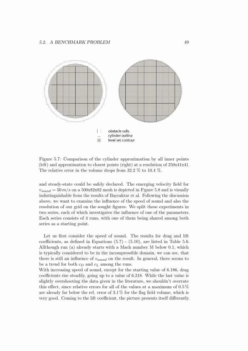
5.2. A BENCHMARK PROBLEM 49
Figure 5.7: Comparison of the cylinder approximation by all inner points(left) and approximation to closest points (right) at a resolution of 250x41x41.The relative error in the volume drops from 32.2 % to 10.4 %.
and steady-state could be safely declared. The emerging velocity field forvsound = 50m/s on a 500x82x82 mesh is depicted in Figure 5.8 and is visuallyindistinguishable from the results of Bayraktar et al. Following the discussionabove, we want to examine the influence of the speed of sound and also theresolution of our grid on the sought figures. We split these experiments intwo series, each of which investigates the influence of one of the parameters.Each series consists of 4 runs, with one of them being shared among bothseries as a starting point.
Let us first consider the speed of sound. The results for drag and liftcoefficients, as defined in Equations (5.7) - (5.10), are listed in Table 5.6.Allthough run (a) already starts with a Mach number M below 0.1, whichis typically considered to be in the incompressible domain, we can see, thatthere is still an influence of vsound on the result. In general, there seems tobe a trend for both cD and cL among the runs.With increasing speed of sound, except for the starting value of 6.186, dragcoefficients rise steadily, going up to a value of 6.218. While the last value isslightly overshooting the data given in the literature, we shouldn’t overratethis effect, since relative errors for all of the values at a maximum of 0.5%are already far below the rel. error of 3.1% for the flag field volume, which isvery good. Coming to the lift coefficient, the picture presents itself differently.

50 CHAPTER 5. EXAMPLE RESULTS
Figure
5.8:Velocity
fieldof
theflow
aroundthe
cylinderafter
16swith
aparabolic
inflowprofile
accordingto
Equation
5.5
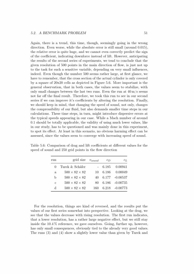
5.2. A BENCHMARK PROBLEM 51
Again, there is a trend, this time, though, seemingly going in the wrongdirection. Even worse, while the absolute error is still small (around 0.015),the relative error is quite huge, and we cannot even correctly predict the signof the coefficient, indicating downforce instead of lift. However, anticipatingthe results of the second series of experiments, we tend to conclude that thegiven resolution of 500 points in the main direction of flow, is just not upto the task for such a sensitive variable, depending on very small influences,indeed. Even though the number 500 seems rather large, at first glance, wehave to remember, that the cross section of the actual cylinder is only coveredby a square of 20x20 cells as depicted in Figure 5.6. More important is thegeneral observation, that in both cases, the values seem to stabilize, withonly small changes between the last two runs. Even the run at 40m/s seemsnot far off the final result. Therefore, we took this run to see in our secondseries if we can improve it’s coefficients by altering the resolution. Finally,we should keep in mind, that changing the speed of sound, not only, changesthe compressibility of our fluid, but also demands smaller time steps in ourcalculations. These time steps, in turn, might introduce dispersive errors atthe typical speeds appearing in our case. While a Mach number of around0.1 should be totally applicable, the validity of using much lower values, likein our study, has to be questioned and was mainly done in this experiment,to spot its effect. At least in this scenario, no obvious harming effect can beassessed, since the values seem to converge with increasing speed of sound.
Table 5.6: Comparison of drag and lift coefficients at different values for thespeed of sound and 250 grid points in the flow direction
run grid size vsound cD cL
0 Turek & Schäfer - 6.185 0.00941a 500× 82× 82 10 6.186 0.00049b 500× 82× 82 40 6.177 -0.00537c 500× 82× 82 80 6.186 -0.00735d 500× 82× 82 160 6.218 -0.00773
For the resolution, things are kind of reversed, and the results put thevalues of our first series somewhat into perspective. Looking at the drag, wesee that the values decrease with rising resolution. The first run indicates,that a lower resolution, has a rather large negative effect, but we still stayinside the 10.4% reference, we gave ourselves. Going, further up, however,has only small consequences, obviously tied to the already very good values.The runs (3) and (4) show a slightly lower value than given by Turek and

52 CHAPTER 5. EXAMPLE RESULTS
Schäfer, with the last one indicating, that it will probably stay in this region,even for higher resolutions. In the end, our error is somewhere close to 1%,which is totally fine. Remembering, that we expect the values to still slightlyincrease for higher speeds of sound and the two effects might potentiallycancel, we are very pleased with the outcome. Going over to the lift, we cansee that the values for higher resolutions are much improved over the onesseen before. Now, we can correctly predict a lifting force on the cylinder,albeit a bit smaller than we hoped for. Also, while the drag coefficient seemsto stabilize among the runs and only varies slightly, the lift coefficient stillshows quite high deviations even for the higher resolutions. Considering,however, the small total error, which is now in the order of 0.005 and the fact,that this is also the instance, where deviations among the compared codes inthe literature is highest, we can still be very satisfied with our results.
Table 5.7: Comparison of drag and lift coefficients for different grid resolutionsat vSound = 40m/s
run grid size vsound cD cL
0 Turek & Schäfer - 6.185 0.009411 250× 41× 41 40 6.609 -0.034012 500× 82× 82 40 6.177 -0.0053743 750× 123× 123 40 6.103 0.0017164 1.000× 164× 164 40 6.114 0.004191
In total, we can say that our results are pretty satisfying. Even though ourcode is at first glance not perfectly suited for the presented drag and liftcalculations, as they heavily depend on correctly resolving the flow at or nearthe boundary, which profits vigorously from having some form of adaptivity,we can still assert a very solid performance in computing both lift and dragvalues, if we can cope with the mandated high resolutions. We can not totallyreplicate the results of Bayraktar et al. but we are in as close proximity, ascan be expected.
5.3 A physical problem
After successfully solving some benchmark problems, which are mainly con-structed for CFD code verification purposes, we now want to look into solvingan actual physical problem with realistic constants and parameters, thatalso involves more complex geometry. Since we cannot expect to accuratelyresolve turbulence at high Reynolds numbers, we looked for an example,

5.3. A PHYSICAL PROBLEM 53
where the Reynolds number is kept below a threshold value of approximately10.000. One area, where these requirements are met, is the flight of insects.Due to their small bodies, Reynolds numbers tend to be in a range of 3.000-5.000. Small insects use active flying techniques with high frequencies ofwing beat, though, but butterflies, in contrast, also show some periods ofgliding. Therefore we decided, to set up a model of a typical butterfly and seewhat we can get out of it. The model is considered to be a proof of concept,only, and was therefore kept relatively simple. To be able to resolve thewings accurately at a reasonable resolution, the thickness of the wings wasemphasized to 0.3mm. The model at hand has a wingspan of approximately38mm. The four symmetric wings are attached to a body of 18mm length.A drawing of the exact model, as well as an isometric view can be seen inFigure 5.10 and Figure 5.9. The model is positioned in the anterior half ofa fluid channel of length 0.1m and is inclined at an angle of attack of 12°.It is simulated on a grid consisting of 192 Million cells, which is by far thebiggest and computationally most expensive case in our work, and clearlyshows the backdrop of a uniform mesh without the possibilities of adaptivity.The exact setup is listed in Table 5.8. The inflow is set to 0.8m/s, which weimagine to be a typical velocity encountered by such an insect, even thoughtheir maximal air speeds can reach much higher values.
Figure 5.9: Isometric view of the simulated butterfly model; Rendered inKeyShot 5 Student Edition
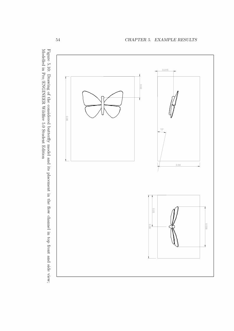
54 CHAPTER 5. EXAMPLE RESULTS
0.038
0.04
0.015
0.06
0.08
0.02
0.03
12°
Figure
5.10:Draw
ingof
theconsidered
butterflymodel
andits
placement
inthe
flowchannel
intop
frontand
sideview
;Modelled
inPro/E
NGIN
EER
Wildfire
5.0Student
Edition
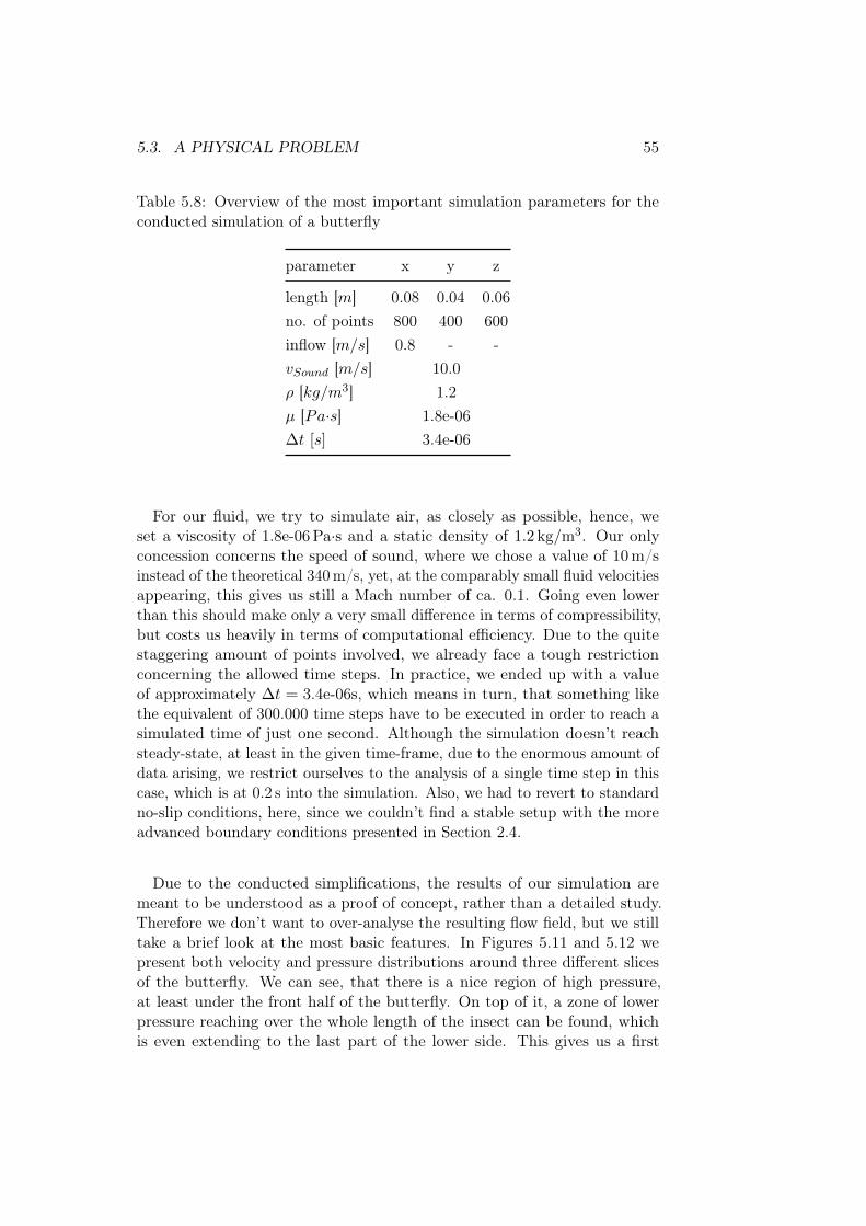
5.3. A PHYSICAL PROBLEM 55
Table 5.8: Overview of the most important simulation parameters for theconducted simulation of a butterfly
parameter x y z
length [m] 0.08 0.04 0.06no. of points 800 400 600inflow [m/s] 0.8 - -vSound [m/s] 10.0ρ [kg/m3] 1.2µ [Pa·s] 1.8e-06∆t [s] 3.4e-06
For our fluid, we try to simulate air, as closely as possible, hence, weset a viscosity of 1.8e-06Pa·s and a static density of 1.2 kg/m3. Our onlyconcession concerns the speed of sound, where we chose a value of 10m/sinstead of the theoretical 340m/s, yet, at the comparably small fluid velocitiesappearing, this gives us still a Mach number of ca. 0.1. Going even lowerthan this should make only a very small difference in terms of compressibility,but costs us heavily in terms of computational efficiency. Due to the quitestaggering amount of points involved, we already face a tough restrictionconcerning the allowed time steps. In practice, we ended up with a valueof approximately ∆t = 3.4e-06s, which means in turn, that something likethe equivalent of 300.000 time steps have to be executed in order to reach asimulated time of just one second. Although the simulation doesn’t reachsteady-state, at least in the given time-frame, due to the enormous amount ofdata arising, we restrict ourselves to the analysis of a single time step in thiscase, which is at 0.2 s into the simulation. Also, we had to revert to standardno-slip conditions, here, since we couldn’t find a stable setup with the moreadvanced boundary conditions presented in Section 2.4.
Due to the conducted simplifications, the results of our simulation aremeant to be understood as a proof of concept, rather than a detailed study.Therefore we don’t want to over-analyse the resulting flow field, but we stilltake a brief look at the most basic features. In Figures 5.11 and 5.12 wepresent both velocity and pressure distributions around three different slicesof the butterfly. We can see, that there is a nice region of high pressure,at least under the front half of the butterfly. On top of it, a zone of lowerpressure reaching over the whole length of the insect can be found, whichis even extending to the last part of the lower side. This gives us a first

56 CHAPTER 5. EXAMPLE RESULTS
indication, that the (simplified) wings actually produce some lift. In thevelocity plots, we can also see, that there is a huge separation going on in themiddle half of the butterfly, that probably stems from the narrow connectionto the clumsy body towards the middle. In contrast, the flow around theoutside of the wings is much cleaner, but the leading edge radius of the wingseems to be too small, for having an attached flow round the upper side ofit. This is no surprise, however, since air is rather viscous at the size of suchanimals, and therefore, the main means of movement is by wing beat, anyhow.Their flight circumstances are probably more comparable to swimming, ratherthan the flight of a large bird. Figure 5.13 shows another view from the sideand top of the butterfly. Employing some stream tracers, we can see thetypical tip vortices forming at the end of the wings, compensating for thepressure difference between upper and lower sides of them. Their inwardrotation, gives us yet another hint at the lift generated by our butterfly. As afinal notice, we are pleased to see, that although at a restricted flight regime,we are able to actually make relevant experiments, in physically simulatedair.
5.4 Unidirectional fluid-motion coupling
There are many interesting problems and real-world applications, that involvesome kind of moving objects, that can only be solved using a method like theone at hand. In this section, we want to give examples for some unidirectionalcoupling of fluid flow with body movement.
Oscillating ball
First, we want to start off with an example of unidirectional coupling. Weconsider a ball oscillating vertically in a horizontal flow field. If we denote thevelocity of the centre of mass of said ball with uM , vM and wM accordingly,the movement of the ball is determined by the equations
vM (t) = 0.5 cos(2t)
uM (t) = wM (t) = 0,(5.11)
representing a sinusoidal oscillation with a total movement range of 1m anda period of π seconds. The ball itself was chosen to have a diameter of 0.4mand its centre of mass (CoM) is located at coordinates (2.0,1.0,1.0), to beginwith. For the horizontal flow, we used the parabolic inflow described inEquation (5.5) again, with a maximal velocity of Um = 2.0m/s this timearound. The setup of the surrounding channel, as well as the most importantsimulation parameters, is shown in Table 5.9. Given this information, we can
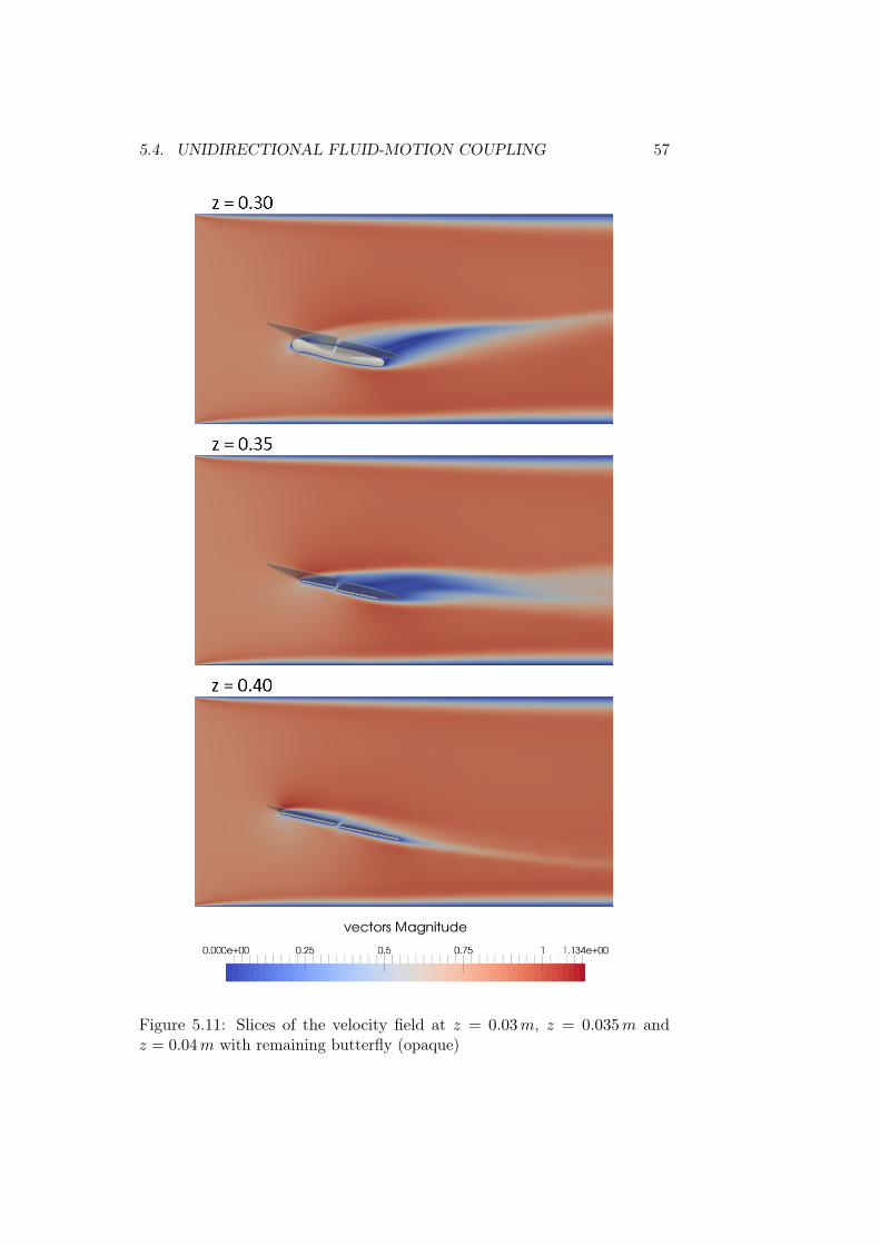
5.4. UNIDIRECTIONAL FLUID-MOTION COUPLING 57
Figure 5.11: Slices of the velocity field at z = 0.03m, z = 0.035m andz = 0.04m with remaining butterfly (opaque)

58 CHAPTER 5. EXAMPLE RESULTS
Figure 5.12: Slices of the pressure field at z = 0.03m, z = 0.035m andz = 0.04m with remaining butterfly (opaque)

5.4. UNIDIRECTIONAL FLUID-MOTION COUPLING 59
Figure 5.13: Tip vortices at the wings as seen from the back and bottom ofthe butterfly; visualized with stream tracers emerging from vertical lines

60 CHAPTER 5. EXAMPLE RESULTS
calculate the Reynolds number as
Re =ρ · U · lµ
≈ 70, (5.12)
where we took the diameter of the ball as our typical length l and the meaninflow velocity U = 4
9Um ≈ 0.9m/s as the reference in terms of velocity.
Table 5.9: Overview of the most important dimensions and simulation para-meters for the oscillating ball
parameter x y z
length [m] 8.0 2.0 2.0no. of points 360 90 90inflow Um [m/s] 2.0 - -CoM [m] (t = 0) 2.0 1.0 1.0vSound [m/s] 20.0ρ [kg/m3] 1.0µ [Pa·s] 0.005∆t [s] ≈ 3.5e-04
With the layout of the simulation in place, we can now look at the resultingflow field. Figure 5.14 shows a clip through the catholicity field at z = 1.0mafter the simulation reached a periodic or quasiperiodic state. At the back ofthe ball a long tail has emerged testifying the sinusoidal movement. The threedifferent pictures in the figure represent the transition from upward movementto downward movement at the upper turning point. In turn the tail changesfrom a lower arc behind the ball to an upper arc. At this particular Reynoldsnumber no vortex street can be found in the trail and the overall impressionis very tidy, just the way we expected it. At higher Reynolds numbers thepicture appears more cluttered and the specific features quickly become muchharder to track. We want to take a look at this behaviour in a differentsetting, next.
Rotating ball
In this simulation, we want to consider a rotating ball in a cavity. Althoughour method doesn’t allow for rotating objects per se, as mentioned in Section4.3, it is obviously possible to do it in the case of a rotationally symmetricobject by moving it in a circular motion around the rotation centre. There is

5.4. UNIDIRECTIONAL FLUID-MOTION COUPLING 61
Figure 5.14: Velocity field of the oscillating ball in horizontal flow at threedifferent time steps; before, in close proximity and after the upper turningpoint of the motion
62 CHAPTER 5. EXAMPLE RESULTS
no inflow in this case, all the fluid movement is generated by the movementof the ball. The movement of the ball, which is placed in the same startingposition, is described by the following set of equations:
uM (t) = 2 cos(2t)
vM (t) = 2 sin(2t)
wM (t) = 0
(5.13)
Together they make for a circular motion of diameter D = 2.0m and a periodof π seconds. We want to perform the simulation at two different viscositiesthis time around, namely at µ = 0.002Pa·s and µ = 0.0005Pa·s, respectively.If we use the magnitude of the movement |uM | = 2.0m/s as a referencevelocity and again, the diameter of the ball, i.e. 0.4m, as reference length,we can calculate the Reynolds number Re as 400 and 1600, correspondingly.In Table 5.10, once again, the most important simulation parameters areoutlined.
Table 5.10: Overview of the most important simulation parameters for therotating ball
parameter x y z
length [m] 4.0 4.0 2.0no. of points 180 180 90inflow [m/s] - - -CoM [m] (t = 0) 2.0 1.0 1.0vSound [m/s] 10.0ρ [kg/m3] 1.0µ [Pa·s] 0.002 / 0.0005∆t [s] ≈ 6.0e-04
Turning our attention to the results, which are depicted in Figures 5.15and 5.16, we make the following observations. Compared to the oscillatingball above, instead of the dead water behind the ball, the trail area nowmakes up for most of the activity. This is obviously due to the movementof the ball now being the only source of fluid flow, compared to the staticbackground flow in the above experiment. Again, the path of the ball canbe very nicely traced in the shape of its trailing velocity field. Already at aReynolds number of 400, we can see vortices forming in this trail area and

5.4. UNIDIRECTIONAL FLUID-MOTION COUPLING 63
Figure 5.15: Velocity field and level set contour of the rotating ball at t = 2.8 s(top) and t = 3.2 s (bottom) and Reynolds number Re = 2000

64 CHAPTER 5. EXAMPLE RESULTS
Figure 5.16: Velocity field and level set contour of the rotating ball at t = 2.8 s(top) and t = 3.2 s (bottom) and Reynolds number Re = 8000

5.5. BIDIRECTIONAL COUPLING 65
moving to the border of the cavity in regular intervals. While at Re 400 wehave very distinct vortices forming over a period of time, at Re 1600 thepicture is a bit different. The flow still has the same basic structure, but nowthe vortices break apart into many small disturbances as soon as they form.Overall the picture is very cluttered. It’s difficult to say if the small scale flowfeatures can still be accurately resolved by our mesh, or if the turbulence isalready high enough to require a much finer grid. Additionally, the maximalvelocity in the trail rises from just below 2.5m/s to nearly 3m/s, althoughthe general shape and length of the trail seem to be very similar. In principle,this is the expected behaviour, though, as a smaller viscosity should meanless fluid is being pulled behind the ball, but at a faster maximum velocity.
5.5 Bidirectional coupling
Having seen two different cases of unidirectional fluid-motion coupling, inthis section, we want to try the possibilities of bidirectional coupling, i.e. ofobjects, that not only influence the surrounding fluid, but are now also directlydriven by the flow. We consider these as examples of what possibilities thereare, always keeping in mind the restrictions mentioned in Chapter 4.
Movement against the stream
With our first example of bidirectional coupling, we want to stay in the samesetting as before, considering a ball in a channel. The basic setting is verysimilar to the oscillating ball discussed above, the only difference being, thatwe now only define an initial velocity of the ball and subsequently lettingthe forces, generated by the flow, act freely upon it. One can imagine theexperiment as a ball being thrown against the wind, being slowed down byit, and eventually changing direction and coming back to its initial position.With this in mind, we want to take a look at our simulation parameters(compare Table 5.11), that were chosen in a way to accommodate this wholeprocess in our given channel. We start of with our ball in the middle of thechannel at coordinates (4.0,1.0,1.0) and a starting velocity of -2.0m/s in xdirection. The fluid is initially at rest and has a relatively high viscosity of0.01 Pa·s to ensure that no detachments or other assymetries occur behind theball, which would push it our of the centre of the channel after the turningpoint is reached. For this experiment, we also fall back to the standarduniform inflow condition at the left boundary of the channel. In addition tothe usual parameters, for the bidirectional coupling, we have to prescribe adensity for the solid object on which our fluid acts. In this case we set thedensity to 30 kg/m3, which gives us a reasonable time and distance, until theeventual change of direction happens.

66 CHAPTER 5. EXAMPLE RESULTS
Figure 5.17: Velocity field and level set contour of a ball moving contrary tothe flow at t = 0.04 s, t = 1.00 s and t = 2.00 s and being slowed down by ituntil near rest

5.5. BIDIRECTIONAL COUPLING 67
Figure 5.18: Velocity field and level set contour of the ball at t = 3.00 s,t = 5.00 s and t = 7.00 s after reaching the turning point and being draggedback by the flow

68 CHAPTER 5. EXAMPLE RESULTS
Table 5.11: Overview of the most important simulation parameters for themovement against the stream case
parameter x y z
length [m] 8.0 4.0 2.0no. of points 360 90 90inflow [m/s] 2.0 - -CoM [m] (t = 0) 4.0 1.0 1.0vSound [m/s] 20.0ρ [kg/m3] 1.0ρs [kg/m3] 30.0µ [Pa·s] 0.01∆t [s] ≈ 3.6e-04
The chronological order of the events is depicted in Figures 5.17 and 5.18,showing once again the velocity field on a clip through the centre plane of thechannel. The first picture shows the initial position of the ball right in thecentre of the channel, just after the experiment started. Due to the suddeninitial movement of the ball, as well as the inflow, we see some sound wavesemerging, that are reflected at the boundaries, but dampen out over time.The second picture is already one second into the experiment. Throughoutthe length of the channel the fluid is already moving at close to the inflowvelocity, with the usual increase at the level of the ball, due to it blockingpart of the channel. Behind the ball (to the right in the pictures), the typicaldrop-shaped trail for low Reynolds numbers has emerged. Looking closer,however, we can spot another trail inside the bigger one, stemming from themotion of the ball itself, that pulls the fluid in its own direction of movementcontrary to the surrounding flow. At two seconds, this inner trail alreadybegins to vanish, indicating that the ball has slowed down quite significantly.Glancing at Figure 5.18 we can see that it has nearly reached the maximaldisplacement on its trajectory. In contrast, the outer drop is still extendingits reach to the back of the channel. At three seconds, we have reachedthe turning point (the exact time is 3.05 s) at coordinates (1.54,1.00,1.00),corresponding to a distance of 2.46m from its initial position. The two layereddrops have merged into one, and the ball starts its voyage back to its origin.From here on the drop-shape begins to shrink, as the ball is accelerated in theopposing direction. At t = 7.00 s it has already gone past the middle of thechannel and is headed towards the outflow with a velocity of 1.07m/s, whichis slowly crawling up to the 2.0m/s of the surrounding flow. The deflection

5.5. BIDIRECTIONAL COUPLING 69
in the cross-section of the channel is still below 1mm in both the y and zdirection. In total, we can attest a first successful test of our bidirectionalcoupling as described in Section 4.4. The observed results, all seem to bevery reasonable, at the least.
Flying butterfly
As a final example, we want to put something together showcasing everythingwe have seen so far packed up in one simulation. We have already seena very complex geometry, with our butterfly model. Once again, we wantto emphasize on the quite ridiculous amount of over 190 Mio. cells beingdeployed, here. Being able to still run such an experiment in a reasonabletime frame of around two to three days gives testimony to the quite insanecomputing powers enabled by modern hardware, as well as the efficiency ofour code, in dealing with such a grid. Up to this point, we have only seen thebutterfly stationary, now, we want to combine this, with the bidirectionalcoupling introduced above, and test, if it produces enough lift to keep itselfup under gravity. In short: let us see if it can fly. We therefore introducea constant gravity acceleration of −9.81 m/s2 in y-direction, additional tothe forces generated by the flow. For the density of the butterfly, we chose avalue of 400 kg/m3, resulting in a mass of ≈ 0.1 g for the whole model, whichseems plausible for a butterfly of this size. The rest of the setup stays asdescribed in Section 4.4 for the stationary case, except for the inflow beingturned up to 2.2m/s this time. Looking at the previous numbers, this shouldgive us the kind of lifting forces needed to overcome the gravity, or at leastfor gliding only slowly to the ground. As a result, of course our Reynoldsnumber goes up to a value of approximately 5000, which should result ina much livelier flow field than before. To stay in the same kind of region,concerning the Mach number we also increased our speed of sound to 20m/s,dealing with the fact, that this further decreases our time steps to around1.9e-06 s.
Now, when activating the forces making up our coupling right from thebeginning, the butterfly starts to fall down right away, as there is no time forthe flow to build up any significant forces counteracting it, and there is noway they will be able to catch it once it reaches a certain velocity. To adjustto these circumstances, we initially simulate statically for a period of 0.05 s,and only enable both the gravity, as well as the fluid forces after this initial,neutralized phase. Having declared the setup of our final experiment, we nowwant to answer our initial question: Can the wings actually produce enoughlift to make the butterfly stay in the air?
Looking at the resulting time line depicted in Figures 5.19 and 5.20, wecan answer the question. In the second picture, we can see that the butterfly
70 CHAPTER 5. EXAMPLE RESULTS
Table 5.12: Overview of the most important simulation parameters for theflying butterfly
parameter x y z
length [m] 0.08 0.04 0.06no. of points 800 400 600inflow [m/s] 2.2 - -vSound [m/s] 20.0ρ [kg/m3] 1.2ρs [kg/m3] 400.0µ [Pa·s] 1.8e-06∆t [s] 1.9e-06
indeed moved slightly upwards (as well as to the back) from its initial position.Looking at the output, we see a lifting force of around 110% the force enactedby gravity. Looking at the following time steps, though, we see, that afterthis initial rise, the model comes back down again, slowly sliding closer tothe ground. This behaviour is quite natural in our setting. The longer oursimulation goes on, the faster our butterfly becomes in the flow direction,therefore decreasing the difference to the velocity of the fluid myself. Withthis effective air speed of the butterfly shrinking, obviously, the lift producedby its wings also drops and our model starts to go back down. Looking a bitcloser at the actual flow around the insect, we can also very clearly detect thepredicted effects of the increase in the Reynolds number. There are a lot ofvortices separating from the body part of the butterfly giving it a far wilderlook compared to before. In total, we are very pleased with the outcome ofthis experiment, proving the very good stability, we actually have with ourcoupling.
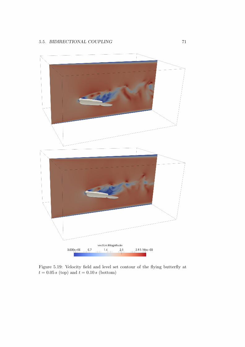
5.5. BIDIRECTIONAL COUPLING 71
Figure 5.19: Velocity field and level set contour of the flying butterfly att = 0.05 s (top) and t = 0.10 s (bottom)
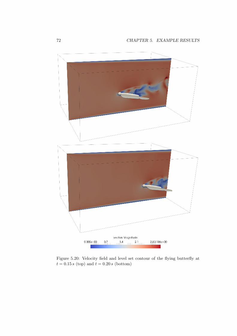
72 CHAPTER 5. EXAMPLE RESULTS
Figure 5.20: Velocity field and level set contour of the flying butterfly att = 0.15 s (top) and t = 0.20 s (bottom)

Chapter 6
Outlook
Summary
The goal of this work has been to examine the behaviour of the unidirec-tional, as well as the bidirectional coupling of of a fluid simulation to movingobstacles, in a compressible setting. Indeed, we can report a very stableperformance of our implemented code, especially concerning initial condi-tions. Even sudden movements, at the beginning of a simulation, like inour first example of the bidirectional coupling, only lead to some expectedpressure waves emerging from the object, superimposing our picture, untilthey eventually dampen out. In conclusion we have implemented an efficient,explicit, compressible flow solver, that meets the demanded requirements.Complex geometry can be directly imported via stl models from externalsoftware, and is translated to our level set approach. In our computationalbenchmarks, when approximating a fine reference solution, we could showan order of convergence of 1.79 and 1.46 for the velocity and pressure fields,respectively. With a parallel efficiency of 80.4% at a 16-fold increase of theinvolved processors, we have a highly parallel software, at hand. Finally, weshowed the applicability of the algorithm to a physically relevant problem,including the (simplified) geometry of a butterfly, which is especially hard toresolve. The staggering amount of over 190 Million cells that we could use,shows the efficiency of our explicit update scheme, concerning the computingcosts per time steps. The results for the computed drag and lift forces whereplausible in all cases.
There are some limitations as well, however, that we don’t want to conceal.The iterated transport of the level set function lead to severe problemswith mass loss, at first. In the case of translations, we could overcome thisproblem by exploiting the structure of our grid, but we couldn’t find a wayto generalize this trick to rotations. Additionally, we saw that a Cartesiangrid, despite its advantages, requires extremely many points to resolve any
73

74 CHAPTER 6. OUTLOOK
really complex geometry, which might harm our accuracy, when calculatingthe forces, needed in a bidirectional coupling. All-in-all we can still be verypleased with our results.
Outlook
Despite the efforts undertaken, there are obviously many ways, in which thepresented methods could be further improved. A fairly simple generalization,would be, to allow for multiple objects, moving independently of each other.Since the distance to a collection of objects, is the minimum over the distancesto each individual object, the evaluation of the level-set function would beeasy, even if each object was represented by it’s own version of it. The onlychanges required would concern the infrastructure of the code.
Regarding more substantial extensions, there is the obvious generalizationto a full fluid-structure interaction, by coupling the simulation to a structuralFEM solver, which we set as a kind of far-term goal in the beginning ofour project. Besides this, there is another improvement, that would requireequally substantial effort to be realized. An adaptive grid, where regionsaround objects could receive a finer resolution, to spare some computationalcosts in the rest of the scene, would help us to reduce the needed amountof cells. Yet, to reap the full potential of this investment, we would alsohave to implement local time stepping, because otherwise the smallest cellsin our scene would dictate the admissible time step over the whole domain,limiting the gain in efficiency. Together with the many times increasedeffort in handling the parallelization, there is quite some work to make animprovement along this path.

75
Acknowledgements
Obviously, the present thesis could not have been finished without the helpand support of many people in the background. At this point I want to thankthem all, for giving me the opportunity to work on this project, which provedto be very rewarding and teaching at the same time.
First of all I want to thank Prof. Dr. Griebel for handing me over thisinteresting topic and his great support in terms of giving ideas and outlininginteresting directions. I also want to thank Prof. Dr. Schweitzer for takingover the role of the second assessor. On the same note I have to thank MarkusBurkow, who introduced me to the NaSt3DGP fluid solver, took care of allof my day-to-day needs, and shared a lot of helpful insights along the way.
For providing me with all the infrastracture, especially the possibility to usethe Atacama compute cluster, I thank the staff of the Institute of NumericalSimulation at the University of Bonn.
A major thanks goes to all members of the BRS-Motorsport Team at UASSankt Augustin, who played a major part in getting me interested in fluidproblems, to begin with, and with whom I had two very special seasons ofcompeting in the Formula Student, always paired with a lot of fun.
Additionally, I thank Sren Behr and my father Erwin for proof readingthis thesis and giving valuable feedback on many points.
Finally, I want to thank my family for supporting me relentlessly, through-out my studies, and enabling all of this in the first place. Without the ongoingsupport of all of you nothing of this would be possible.

76 CHAPTER 6. OUTLOOK
List of Figures
2.1 Schematic overview of the required communication betweenfour neighbouring processors in 2D, using tree layers of ghostcells and one corner cell . . . . . . . . . . . . . . . . . . . . . 20
3.1 Step 1: Stl model of a motorcycle helmet, left half visualizedwith edges . . . . . . . . . . . . . . . . . . . . . . . . . . . . . 27
3.2 Step 2: Flag field threshold of a motorcycle helmet, left halfvisualized with edges . . . . . . . . . . . . . . . . . . . . . . . 27
3.3 Step 3: Level set contour of a motorcycle helmet, left halfvisualized with edges . . . . . . . . . . . . . . . . . . . . . . . 28
4.1 Basic idea of the Semi-Lagrangian ansatz . . . . . . . . . . . 32
5.1 Velocity field of a driven cavity on a 256x256 grid at Re = 100(left) and Re = 400 (right) and U = 1m/s; stopped aftersimulated time of 24 s. The purple crosses mark the vortexcentres found by [Hou+95]. . . . . . . . . . . . . . . . . . . . 38
5.2 Progression of L2 errors for the velocity U and the pressure pcompared to the respective convergence order on a logarithmicscale . . . . . . . . . . . . . . . . . . . . . . . . . . . . . . . . 41
5.3 Clip through the velocity field of the conducted driven cavityexperiment for strong scaling on a cluster. . . . . . . . . . . . 42
5.4 Speedup (top) and efficiency (bottom) plot for up to 512 coreson a CPU-cluster . . . . . . . . . . . . . . . . . . . . . . . . . 43
5.5 Setup and main dimensions of the 3D-1Z cylinder benchmarkwith circular cross-section according to Turek and Schäfer;taken from [TS96] . . . . . . . . . . . . . . . . . . . . . . . . 45
5.6 Approximation of the cylinder outline by the flag field andthe level set contour at a resolution of 250x41x41 (left) and500x82x82 (right) . . . . . . . . . . . . . . . . . . . . . . . . . 47
5.7 Comparison of the cylinder approximation by all inner points(left) and approximation to closest points (right) at a resolutionof 250x41x41. The relative error in the volume drops from32.2 % to 10.4 %. . . . . . . . . . . . . . . . . . . . . . . . . . 49
77

78 LIST OF FIGURES
5.8 Velocity field of the flow around the cylinder after 16 s with aparabolic inflow profile according to Equation 5.5 . . . . . . . 50
5.9 Isometric view of the simulated butterfly model; Rendered inKeyShot 5 Student Edition . . . . . . . . . . . . . . . . . . . 53
5.10 Drawing of the considered butterfly model and its placementin the flow channel in top front and side view; Modelled inPro/ENGINEER Wildfire 5.0 Student Edition . . . . . . . . . 54
5.11 Slices of the velocity field at z = 0.03m, z = 0.035m andz = 0.04m with remaining butterfly (opaque) . . . . . . . . . 57
5.12 Slices of the pressure field at z = 0.03m, z = 0.035m andz = 0.04m with remaining butterfly (opaque) . . . . . . . . . 58
5.13 Tip vortices at the wings as seen from the back and bottomof the butterfly; visualized with stream tracers emerging fromvertical lines . . . . . . . . . . . . . . . . . . . . . . . . . . . . 59
5.14 Velocity field of the oscillating ball in horizontal flow at threedifferent time steps; before, in close proximity and after theupper turning point of the motion . . . . . . . . . . . . . . . 61
5.15 Velocity field and level set contour of the rotating ball att = 2.8 s (top) and t = 3.2 s (bottom) and Reynolds numberRe = 2000 . . . . . . . . . . . . . . . . . . . . . . . . . . . . . 63
5.16 Velocity field and level set contour of the rotating ball att = 2.8 s (top) and t = 3.2 s (bottom) and Reynolds numberRe = 8000 . . . . . . . . . . . . . . . . . . . . . . . . . . . . . 64
5.17 Velocity field and level set contour of a ball moving contraryto the flow at t = 0.04 s, t = 1.00 s and t = 2.00 s and beingslowed down by it until near rest . . . . . . . . . . . . . . . . 66
5.18 Velocity field and level set contour of the ball at t = 3.00 s,t = 5.00 s and t = 7.00 s after reaching the turning point andbeing dragged back by the flow . . . . . . . . . . . . . . . . . 67
5.19 Velocity field and level set contour of the flying butterfly att = 0.05 s (top) and t = 0.10 s (bottom) . . . . . . . . . . . . 71
5.20 Velocity field and level set contour of the flying butterfly att = 0.15 s (top) and t = 0.20 s (bottom) . . . . . . . . . . . . 72

List of Tables
2.1 Applied differencing sequence for the MacCormack scheme;modelled on the corresponding table in [THR76] . . . . . . . 14
5.1 Relative L2 errors for different resolutions compared to a800x800 reference grid . . . . . . . . . . . . . . . . . . . . . . 40
5.2 Speedup and efficiency of a three dimensional driven cavitysimulation on up to 512 cores . . . . . . . . . . . . . . . . . . 44
5.3 Grid size and speed of sound of the different simulation runs;× marks performed runs . . . . . . . . . . . . . . . . . . . . . 46
5.4 Rel. error of the cylinder volume at different grid resolutions 475.5 Rel. error of the cylinder volume computed with the refined
method, motivated by closest points . . . . . . . . . . . . . . 485.6 Comparison of drag and lift coefficients at different values for
the speed of sound and 250 grid points in the flow direction . 515.7 Comparison of drag and lift coefficients for different grid resol-
utions at vSound = 40m/s . . . . . . . . . . . . . . . . . . . . 525.8 Overview of the most important simulation parameters for the
conducted simulation of a butterfly . . . . . . . . . . . . . . . 555.9 Overview of the most important dimensions and simulation
parameters for the oscillating ball . . . . . . . . . . . . . . . . 605.10 Overview of the most important simulation parameters for the
rotating ball . . . . . . . . . . . . . . . . . . . . . . . . . . . . 625.11 Overview of the most important simulation parameters for the
movement against the stream case . . . . . . . . . . . . . . . 685.12 Overview of the most important simulation parameters for the
flying butterfly . . . . . . . . . . . . . . . . . . . . . . . . . . 70
79

80 LIST OF TABLES

Literature
[Bat00] G. Batchelor. An Introduction to Fluid Dynamics.Cambridge Mathematical Library. Cambridge Univer-sity Press, 2000. isbn: 978-0521663960.
[BM77] W. Briley and H. McDonald. ‘Solution of the multidi-mensional compressible Navier-Stokes equations by ageneralized implicit method’. In: Journal of Compu-tational Physics 24.4 (1977), pp. 372–397. doi: http://dx.doi.org/10.1016/0021-9991(77)90029-8.
[BMT12] E. Bayraktar, O. Mierka and S. Turek. ‘BenchmarkComputations of 3D Laminar Flow Around a Cylinderwith CFX, OpenFOAM and FeatFlow’. In: Int. J.Comput. Sci. Eng. 7.3 (July 2012), pp. 253–266. doi:http://dx.doi.org/10.1504/IJCSE.2012.048245.
[BW78] R. M. Beam and R. F. Warming. ‘An ImplicitFactored Scheme for the Compressible Navier-StokesEquations’. In: AIAA Journal 16 (Apr. 1978), pp. 393–402. doi: http://dx.doi.org/10.2514/3.60901).
[Cho68] A. J. Chorin. ‘Numerical solution of the Navier-Stokesequations’. In:Mathematics of Computation 22 (1968),pp. 745–762. doi: http://dx.doi.org/10.1090/S0025-5718-1968-0242392-2.
[Cro02] R. Croce. ‘Ein paralleler, dreidimensionaler Navier-Stokes-Löser für inkompressible Zweiphasenströmun-gen mit Oberflächenspannung, Hindernissen und dy-namischen Kontaktflächen’. MA thesis. Institut fürAngewandte Mathematik, Universität Bonn, 2002.
[Cro10] R. Croce. ‘Numerische Simulation der Interaktion voninkompressiblen Zweiphasenströmungen mit Starrkör-pern in drei Raumdimensionen’. PhD thesis. Institutfür Numerische Simulation, Universität Bonn, 2010.
81

82 LITERATURE
[Enr+02] D. Enright et al. ‘A Hybrid Particle Level Set Methodfor Improved Interface Capturing’. In: Journal ofComputational Physics 183.1 (2002), pp. 83–116. doi:http://dx.doi.org/10.1006/jcph.2002.7166.
[FP08] J. Ferziger and M. Perić. Numerische Strömungsmech-anik. Springer Berlin Heidelberg, 2008. isbn: 978-3540675860. doi: http://dx.doi.org/10.1007/978-3-540-68228-8.
[GDN98] M. Griebel, T. Dornseifer and T. Neunhoeffer. Nu-merical Simulation in Fluid Dynamics, a PracticalIntroduction. SIAM, Philadelphia, 1998. isbn: 978-3528067618.
[GGS82] U. Ghia, K. Ghia and C. Shin. ‘High-Re solutions forincompressible flow using the Navier-Stokes equationsand a multigrid method’. In: Journal of Computa-tional Physics 48.3 (1982), pp. 387–411. doi: http://dx.doi.org/10.1016/0021-9991(82)90058-4.
[Ghi+10] U. Ghia et al. ‘The AIAA Code Verification Project -Test cases for CFD Code Verification’. In: AmericanInstitute of Aeronautics & Astronautics AIAA (2010).doi: http://dx.doi.org/10.2514/6.2010-125.
[Gur81] M. E. Gurtin. An Introduction to Continuum Mechan-ics. Mathematics in Science and Engineering. Elsevier,1981. isbn: 978-0123097507.
[Hou+95] S. Hou et al. ‘Simulation of Cavity Flow by the LatticeBoltzmann Method’. In: Journal of ComputationalPhysics 118.2 (1995), pp. 329–347. doi: http://dx.doi.org/10.1006/jcph.1995.1103.
[HS12] S. Haeri and J. Shrimpton. ‘On the applicationof immersed boundary, fictitious domain and body-conformal mesh methods to many particle multiphaseflows’. In: International Journal of Multiphase Flow40 (2012), pp. 38–55. doi: http://dx.doi.org/10.1016/j.ijmultiphaseflow.2011.12.002.
[KT00] A. Kurganov and E. Tadmor. ‘New high-resolutioncentral schemes for nonlinear conservation laws andconvection-diffusion equations’. In: Journal of Com-putational Physics 160.1 (2000), pp. 214–282.

LITERATURE 83
[Lee79] B. van Leer. ‘Towards the ultimate conservative differ-ence scheme. V. A second-order sequel to Godunov’smethod’. In: Journal of Computational Physics 32.1(1979), pp. 101–136. doi: http://dx.doi.org/10.1016/0021-9991(79)90145-1.
[LFO06] F. Lossaso, R. Fedkiw and S. Osher. ‘Spatially Ad-aptive Techniques for Level Set Methods and Incom-pressible Flow’. In: Computers & Fluids 35.10 (Dec.2006), pp. 995–1010. doi: http://dx.doi.org/10.1016/j.compfluid.2005.01.006.
[LL87] L. Landau and E. Lifshitz. Fluid Mechanics (SecondEdition). Second Edition. Vol. 6. Course of TheoreticalPhysics. Pergamon, 1987. isbn: 978-0080339337. doi:http://dx.doi.org/10.1016/B978-0-08-033933-7.50001-5.
[LW60] P. Lax and B. Wendroff. ‘Systems of conservationlaws’. In: Communications on Pure and Applied Math-ematics 13 (2 1960), pp. 217–237. doi: http://dx.doi.org/10.1002/cpa.3160130205.
[Mac03] R. W. MacCormack. ‘The Effect of Viscosity in Hyper-velocity Impact Cratering’. In: Journal of Spacecraftand Rockets 40 (2003). Reprinted from AIAA Paper69-354, 1969, pp. 757–763. doi: http://dx.doi.org/10.2514/2.6901.
[Mac71] R. W. MacCormack. ‘Numerical Solution of the In-teraction of a Shock Wave with a Laminar Bound-ary Layer’. In: vol. 8. Proceedings of the SecondInternational Conference on Numerical Methods inFluid Dynamics. Springer-Verlag, 1971. doi: http://dx.doi.org/10.1007/3-540-05407-3_24.
[Mac82] R. W. MacCormack. ‘A Numerical Method for Solvingthe Equations of Compressible Viscous Flow’. In:AIAA Journal 20 (1982), pp. 1275–1281. doi: http://dx.doi.org/10.2514/3.51188.
[Mac85] R. W. MacCormack. Current Status of NumericalSolutions of the Navier-Stokes Equations. AIAA 23rdAerodpace Sciences Meeting. Jan. 1985. doi: http://dx.doi.org/10.2514/6.1985-32.

84 LITERATURE
[Mac93] R. W. MacCormack. ‘A Perspective on a QuarterCentury of CFD Research’. In: AIAA Journal 3291(1993), p. 15. doi: http://dx.doi.org/10.2514/6.1993-3291.
[OF01] S. Osher and R. P. Fedkiw. ‘Level Set Methods: AnOverview and Some Recent Results’. In: Journal ofComputational Physics 169.2 (2001), pp. 463–502. doi:http://dx.doi.org/10.1006/jcph.2000.6636.
[OF03] S. Osher and R. P. Fedkiw. Level set methods anddynamic implicit surfaces. Vol. 153. Springer Verlag,2003. doi: http://dx.doi.org/10.1007/3-540-05407-3_24.
[OS88] S. Osher and J. A. Sethian. ‘Fronts Propagatingwith Curvature-Dependent Speed: Algorithms Basedon Hamilton-Jacobi Formulations’. In: Journal ofComputational Physics 79 (Nov. 1988), pp. 12–49.doi: http://dx.doi.org/10.1016/0021-9991(88)90002-2.
[OT02] W. Oberkampf and T. Trucano. Verification andValidation in Computational Fluid Dynamics. Mar.2002. doi: http://dx.doi.org/10.1016/S0376-0421(02)00005-2.
[PH06] A. Perrin and H. H. Hu. ‘An Explicit Finite-differenceScheme for Simulation of Moving Particles’. In:Journal of Computational Physics 212.1 (Feb. 2006),pp. 166–187. doi: http://dx.doi.org/10.1007/1-4020-4977-3_17.
[SSO94] M. Sussman, P. Smereka and S. Osher. ‘A Level SetApproach for Computing Solutions to IncompressibleTwo-Phase Flow’. In: Journal of Computational Phys-ics 114.1 (1994), pp. 146–159. doi: http://dx.doi.org/10.1006/jcph.1994.1155.
[THR76] J. Tannehill, T. L. Holst and J. V. Rakich. ‘NumericalComputation of Two-Dimensional Viscous Blunt BodyFlows with an Impinging Shock’. In: AIAA Journal14.2 (1976), pp. 204–211. doi: http://10.1016/j.jcp.2005.06.021.
[TS96] S. Turek and M. Schäfer. Recent Benchmark Com-putations of Laminar Flow Around a Cylinder. 1996.doi: http://dx.doi.org/10.1007/978-3-322-89849-4_39.

LITERATURE 85
[Wen08] J. Wendt. Computational Fluid Dynamics: An In-troduction. A von Karman Institute book. SpringerBerlin Heidelberg, 2008. isbn: 978-3540850564.
[Wes01] P. Wesseling. Principles of Computational Fluid Dy-namics. Lecture Notes in Computer Science. Springer,2001. isbn: 978-3540678533.
[Whi91] F. White. Viscous Fluid Flow. McGraw-Hill seriesin mechanical engineering. McGraw-Hill, 1991. isbn:978-0070697126.