An exchange flow between the Okhotsk Sea and the North Pacificdriven by the East Kamchatka Current

Shinichiro Kida1 and Bo Qiu2

Received 24 September 2013; revised 5 November 2013; accepted 20 November 2013.

[1] A new mechanism for driving the water mass exchange between the Okhotsk Sea andthe North Pacific is presented. This exchange flow originates from the East KamchatkaCurrent (EKC), a western boundary current of the subpolar gyre, and occurs through thetwo deepest straits of the Kuril island chain, the Kruzenshtern and Bussol straits. An inflowtoward the Okhotsk Sea occurs at the northern Kruzenshtern strait and an outflow towardthe North Pacific occurs at the southern Bussol strait. By using the Kelvin’s Circulationtheorem around the island between the two straits, we show that the transport of theexchange flow entering the Okhotsk Sea is determined such that the frictional stressesaround the island exerted by the bifurcated EKC integrate to zero. This forcing mechanismis different from the dynamical framework of the widely used ‘‘Island rule.’’ Both ananalytical analysis and 1.5-layer model experiments demonstrate that the strait width, lateralviscosity, and island geometry are controlling parameters for the exchange flow transportbecause they affect the magnitude and length scales of the frictional stresses. Inertia of theEKC decreases the exchange flow by enhancing the frictional stress along the northern coastof the Kuril island. Model experiments with realistic topography further reveal that whilethe steep continental slopes have minor impact on the exchange flow transport, thesubsurface peninsula located east of the Kuril island works to decrease the exchange flowby altering the length scale of the frictional stresses and enabling the EKC to flow past theisland.

Citation: Kida, S., and B. Qiu (2013), An exchange flow between the Okhotsk Sea and the North Pacific driven by the EastKamchatka Current, J. Geophys. Res. Oceans, 118, doi:10.1002/2013JC009464.

1. The Water Mass Exchange Between theOkhotsk Sea and the North Pacific

[2] The Okhotsk Sea is a marginal sea located at thenorth-west corner of the North Pacific. While this sea coversan area of more than 43105 km2, it is topographically sepa-rated from the North Pacific by the Kuril island chain. Thereare only two major gaps, the Kruzenshtern and Bussolstraits, where the island chain permits an exchange flow(Figure 1). The Kuril island chain is therefore analogous to athin wall that is only about 30 km wide zonally but a thou-sand kilometer long meridionally. While the magnitude ofthe exchange flow is limited, this flow plays an importantrole in the North Pacific from the regional to basin scale

circulations. The Okhotsk Sea water is considered one of themajor sources of the North Pacific intermediate water[Talley, 1993; Yasuda, 1997] and iron that enables the highproductivity in the region [Nishioka et al., 2007].

[3] The exchange flow between the Okhotsk Sea and theNorth Pacific originates from the East Kamchatka Current(EKC) [Yasuda et al., 2002]. The EKC is a western bound-ary current of the North Pacific subpolar gyre with a trans-port of about 10–11 Sv [Verkhunov and Tkachenko, 1992].While part of the EKC enters the Okhotsk Sea, the majorityof this flow continues along the eastern side of the islandchain from the Kamchatka Peninsula to the Island of Hok-kaido as a western boundary current of the North Pacificand becomes the Oyashio [Yasuda et al., 2002]. Theexchange flow between the Okhotsk Sea and the NorthPacific is observed to occur mainly across two major gapswhere the island chain cracks more than 1000 m deep and40 km wide. An inflow toward the Okhotsk Sea occurs atthe Kruzenshtern Strait and an outflow toward the NorthPacific occurs at the Bussol strait [Katsumata et al., 2001,2004]. While variability of this exchange flow on the sea-sonal and tidal time scales has been observed, past studiessuggest its annual averaged transport to be around 3–5 Sv[Yasuda et al., 2002; Nakamura and Awaji, 2004; Katsu-mata and Yasuda, 2010; Ohshima et al., 2010].

1Earth Simulator Center, Japan Agency for Marine-Earth Science andTechnology, Yokohama, Japan.

2Department of Oceanography, University of Hawaii at Manoa,Honolulu, Hawaii

Corresponding author: S. Kida, Earth Simulator Center, Japan Agencyfor Marine-Earth Science and Technology, 3173-25 Showa-machi,Kanazawa-ku Yokohama, Kanagawa 236-0001, Japan. (kidas@jamstec.go.jp)

©2013. American Geophysical Union. All Rights Reserved.2169-9275/13/10.1002/2013JC009464

1

JOURNAL OF GEOPHYSICAL RESEARCH: OCEANS, VOL. 118, 1–12, doi:10.1002/2013JC009464, 2013

1.1. The Mechanism of the Water Mass Exchange

[4] What are the main processes that drive the exchangeflow between the Okhotsk Sea and the North Pacific?

Understanding its mechanism is important not only forunderstanding the oceanic environment of the Okhotsk Seaand its impact on the North Pacific but also for properlysimulating this exchange flow in general ocean circulationnumerical models. Latest high-resolution general circula-tion models (GCM) are only just beginning to resolve thewidth of the straits and permit an exchange flow.

[5] Katsumata and Yasuda [2010] and Ohshima et al.[2010] recently found that the transport of the exchangeflow is likely correlated with that estimated from the Islandrule [Godfrey, 1989] on the seasonal cycle. These studiesimply that the open ocean winds are remotely driving theexchange flow. However, their studies also find the Islandrule overestimating the transport by 1 order of magnitude.Since the original Island rule aims to estimate the magni-tude of an exchange flow around an isolated island that isof planetary scale, direct application of such theory to theKuril island chain may have been inappropriate. Moreover,the Island rule is based on a steady state assumption and isnot applicable for the seasonal time scale. While the con-nection between the open ocean winds and the exchangeflow may be qualitatively plausible, the actual mechanismthat drives the exchange flow is still an open question.

1.2. The Goal of This Paper

[6] In this paper, we propose that the primary forcing agentof the exchange flow is the EKC. Since the EKC is a westernboundary current of the subpolar gyre of the North Pacific,this EKC-driven mechanism is in line with the idea that theexchange flow is remotely driven by the open ocean winds.By using the Kelvin’s Circulation Theorem, we show that the

140W 150 160 170 180 170 160 150 140 130 120W35

40

45

50

55

60[N]

East Kamchatka Current North Pacific

OkhotskSea

147 148 149 150 151 152 153 154 155 15645

46

47

48

49

[m]

8000

6000

4000

2000

0

KruzenshternStrait

BussolStrait

Exchange Flow

(a)

(b)

Figure 1. (a) The bathymetry and coastlines of the Okhotsk Sea and the North Pacific. The East Kam-chatka Current flows along the Kuril island chain. (b) A closer look of the Kuril island chain. Theexchange flow occurs through the Kruzenshtern strait and Bussol strait. Bathymetric contours shallowerthan 1000 m are drawn in black solid lines every 250 m.

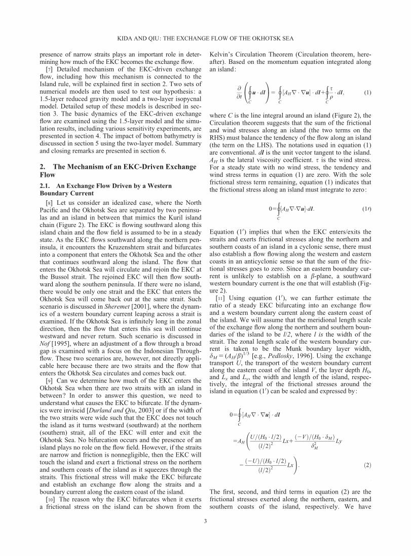
Figure 2. A schematic showing an exchange flow, theEKC, the Okhotsk Sea, and the North Pacific. Modelparameters and the line integral C used in equation (1) arealso shown.

KIDA AND QIU: THE EXCHANGE FLOW OF THE OKHOTSK SEA

2

presence of narrow straits plays an important role in deter-mining how much of the EKC becomes the exchange flow.

[7] Detailed mechanism of the EKC-driven exchangeflow, including how this mechanism is connected to theIsland rule, will be explained first in section 2. Two sets ofnumerical models are then used to test our hypothesis : a1.5-layer reduced gravity model and a two-layer isopycnalmodel. Detailed setup of these models is described in sec-tion 3. The basic dynamics of the EKC-driven exchangeflow are examined using the 1.5-layer model and the simu-lation results, including various sensitivity experiments, arepresented in section 4. The impact of bottom bathymetry isdiscussed in section 5 using the two-layer model. Summaryand closing remarks are presented in section 6.

2. The Mechanism of an EKC-Driven ExchangeFlow

2.1. An Exchange Flow Driven by a WesternBoundary Current

[8] Let us consider an idealized case, where the NorthPacific and the Okhotsk Sea are separated by two peninsu-las and an island in between that mimics the Kuril islandchain (Figure 2). The EKC is flowing southward along thisisland chain and the flow field is assumed to be in a steadystate. As the EKC flows southward along the northern pen-insula, it encounters the Kruzenshtern strait and bifurcatesinto a component that enters the Okhotsk Sea and the otherthat continues southward along the island. The flow thatenters the Okhotsk Sea will circulate and rejoin the EKC atthe Bussol strait. The rejoined EKC will then flow south-ward along the southern peninsula. If there were no island,there would be only one strait and the EKC that enters theOkhotsk Sea will come back out at the same strait. Suchscenario is discussed in Sheremet [2001], where the dynam-ics of a western boundary current leaping across a strait isexamined. If the Okhotsk Sea is infinitely long in the zonaldirection, then the flow that enters this sea will continuewestward and never return. Such scenario is discussed inNof [1995], where an adjustment of a flow through a broadgap is examined with a focus on the Indonesian Through-flow. These two scenarios are, however, not directly appli-cable here because there are two straits and the flow thatenters the Okhotsk Sea circulates and comes back out.

[9] Can we determine how much of the EKC enters theOkhotsk Sea when there are two straits with an island inbetween? In order to answer this question, we need tounderstand what causes the EKC to bifurcate. If the dynam-ics were inviscid [Durland and Qiu, 2003] or if the width ofthe two straits were wide such that the EKC does not touchthe island as it turns westward (southward) at the northern(southern) strait, all of the EKC will enter and exit theOkhotsk Sea. No bifurcation occurs and the presence of anisland plays no role on the flow field. However, if the straitsare narrow and friction is nonnegligible, then the EKC willtouch the island and exert a frictional stress on the northernand southern coasts of the island as it squeezes through thestraits. This frictional stress will make the EKC bifurcateand establish an exchange flow along the straits and aboundary current along the eastern coast of the island.

[10] The reason why the EKC bifurcates when it exertsa frictional stress on the island can be shown from the

Kelvin’s Circulation Theorem (Circulation theorem, here-after). Based on the momentum equation integrated alongan island:

@

@t

þC

u � dl

0@

1A5

þC

AHr � ru½ � � dl1

þC

sq� dl; (1)

where C is the line integral around an island (Figure 2), theCirculation theorem suggests that the sum of the frictionaland wind stresses along an island (the two terms on theRHS) must balance the tendency of the flow along an island(the term on the LHS). The notations used in equation (1)are conventional. dl is the unit vector tangent to the island.AH is the lateral viscosity coefficient. s is the wind stress.For a steady state with no wind stress, the tendency andwind stress terms in equation (1) are zero. With the solefrictional stress term remaining, equation (1) indicates thatthe frictional stress along an island must integrate to zero:

05

þC

AHr�ru½ ��dl: (10)

Equation (10) implies that when the EKC enters/exits thestraits and exerts frictional stresses along the northern andsouthern coasts of an island in a cyclonic sense, there mustalso establish a flow flowing along the western and easterncoasts in an anticyclonic sense so that the sum of the fric-tional stresses goes to zero. Since an eastern boundary cur-rent is unlikely to establish on a b-plane, a southwardwestern boundary current is the one that will establish (Fig-ure 2).

[11] Using equation (10), we can further estimate theratio of a steady EKC bifurcating into an exchange flowand a western boundary current along the eastern coast ofthe island. We will assume that the meridional length scaleof the exchange flow along the northern and southern boun-daries of the island to be l/2, where l is the width of thestrait. The zonal length scale of the western boundary cur-rent is taken to be the Munk boundary layer width,dM 5 (AH/b)1/3 [e.g., Pedlosky, 1996]. Using the exchangetransport U, the transport of the western boundary currentalong the eastern coast of the island V, the layer depth H0,and Lx and Ly, the width and length of the island, respec-tively, the integral of the frictional stresses around theisland in equation (10) can be scaled and expressed by:

05

þC

AHr � ru½ � � dl

5AHU=ðH0 � l=2Þ

l=2ð Þ2Lx1

2Vð Þ= H0 � dMð Þd2

M

Ly

22Uð Þ=ðH0 � l=2Þ

l=2ð Þ2Lx

!: 2ð Þ

(2)

The first, second, and third terms in equation (2) are thefrictional stresses exerted along the northern, eastern, andsouthern coasts of the island, respectively. We have

KIDA AND QIU: THE EXCHANGE FLOW OF THE OKHOTSK SEA

3

assumed that the flow along the western coast of the islandis negligible. Equation (2) can then be expressed as:

0516 � Ul3

Lx2V

d3M

Ly; (3)

where equation (3) clearly shows that the Circulation theo-rem requires the magnitude of the exchange flow andisland’s western boundary current to depend on each other.By further using mass conservation (U1V 5 Q), an esti-mate for U is derived:

U5Q

1116ac23; (4)

where a is the aspect ratio of the island, Lx/Ly, and c is thenondimensional width of the strait, l/dM.

[12] Equation (4) shows that the exchange flow U is sen-sitive to two parameters, a and c, and that U decreaseswhen a increases or when c decreases. This sensitivity of Uon c is similar to the sensitivity of a western boundary cur-rent leaping across a gap [Sheremet, 2001]. The sensitivityof U on ac23 is similar to that of the Island rule when an

island is located close to a wall so that friction enhancesalong the northern or southern coasts of an island [Pedloskyet al., 1997]. Pratt and Pedlosky [1998] also discuss therole of friction based on the Island rule but in the absenceof a western boundary current from the upstream. As willbe further clarified in the next subsection, it is the presenceof the western boundary current from the upstream in ourcase that drives the exchange flow in equation (4). For theexchange flow across the Kuril island chain, the EKC andtwo narrow straits enables us to derive equation (4) andevaluate the sensitivity of U more quantitatively. We willdiscuss how this EKC-driven mechanism and the Islandrule are connected next.

2.2. The EKC-Driven Mechanism and the Island Rule

[13] Theoretical studies on flows around an island pro-gressed much on what is known as the Island rule [Godfrey,1989]. In this subsection, we will clarify how the mecha-nism of an EKC-driven exchange flow put forth in section2.1, differ from, and connect to, this theory.

[14] One simple difference is in the forcing agent. Theexchange flow in the EKC-driven mechanism requires aboundary current flowing from the upstream. It does notdepend on whether a wind stress in the open ocean is pres-ent or not. On the other hand, the exchange flow in theIsland rule is

UIR51

qb yN 2ySð Þ

ðyN

yS

ðxW

xE

r3sdx dy; (5)

and requires a wind stress to be present east of an island(gray area in Figure 3a), [Pedlosky, 1996]. It does notdepend, however, on the wind stress or flow field outside ofthis region.

[15] The second difference is that the EKC-driven mech-anism assumes a different way of balancing the frictionalstresses that are exerted around the island. For the EKC-driven mechanism, the frictional stress along the northernand southern coasts of the island balances that along theeastern coast. For the Island rule, the frictional stress balan-ces within the eastern coast of the island. In other words,the frictional stresses along the northern, southern, andwestern coasts of the island are assumed zero while thetotal frictional stress around the whole island is also zero.The assumption that frictional stress balances within theeastern coast of an island is likely to be valid when themeridional length scale of the island is planetary and muchlarger than the zonal length scale of the island.

[16] The third, and most important, difference is that theEKC-driven mechanism considers the wind-drivenSverdrup flow congregating at the northern tip of the islandas an incoming western boundary current (Figure 3b). Nosuch congregation is considered in the Island rule. To clar-ify the relevance of this difference, we begin by discussingthe Island rule in a rectangular basin with a cyclonicwind-driven gyre and an isolated island in the interior(Figure 3a).

[17] As equation (5) shows, the Island rule estimates theflow around an island based on the spatial average of theSverdrup flow east of the island. However, it is also impor-tant to note that equation (5) contains a component of the

(b)

(a)

Wind driven gyre

Circulation driven bythe island

Wind driven gyre

Circulationdriven by the EKC

EKC

yN

yS

yN

yS

XW XE

XW XE

Figure 3. Two ways the open ocean wind drives anexchange flow: (a) the Island rule. The circulation drivenaround the island is determined by the Sverdrup balancewithin the gray area. (b) EKC-driven mechanism. The EKCis driven by the integral of the Sverdrup balance along thegray line.

KIDA AND QIU: THE EXCHANGE FLOW OF THE OKHOTSK SEA

4

wind-driven gyre that the presence of an island has noinfluence on. As mentioned by Pedlosky et al. [1997], thevalidity of equation (5) can be artificially improved by sim-ply increasing the eastern domain size and increasing thecomponent of the Sverdrup flow. What the Island rule illu-minates is how an island perturbs the interior flow fieldfrom that driven in absence of the island. Such island-driven flow is shown as a dotted line in Figure 3a and itsmagnitude at y 5 yN can be estimated by UIR 2 Q, where

Q51

qb

ðXE

XW

r3 sðy5yN Þdx (6)

is the zonally integrated Sverdrup flow along the northernboundary of the island. If the northern boundary of theisland is located where Q is close to zero [e.g., Pedlosky,1994, Figure 3], then the flow around an island is drivensolely due to the Island rule. However, if the meridionallength scale of an island is small, UIR 2 Q is likely smallbecause the difference between the spatial average of thewind stress curl (equation (5)) and that along the northernlatitude of the island (equation (6)) is likely small. Theisland-driven flow would be weak and what equation (5)expresses is simply the zonal transport of a Sverdrup bal-anced wind-driven gyre (the solid lines in Figure 3a). Inthis case of small UIR 2 Q, it is probably best to regard theflow around the island, UIR, as part of the wind-driven gyreand not as a flow driven by the presence of an island anddictated by the Island rule.

[18] The EKC-driven mechanism considers the case whenan island is not an isolated island, but is bounded by twopeninsulas (Figure 3b). In such situation, the Sverdrup wind-driven gyre circulation can no longer simply go around theisland. A western boundary current will establish along thepeninsula instead with a transport of Q at y 5 yN. When thestraits are narrow, this boundary current will touch the islandand drive an EKC-driven exchange flow. Notice that Qwould be dynamically irrelevant in the case of Figure 3a,but in the presence of a peninsula, it will interact directlywith the island and affect the magnitude of the exchangeflow. Such role of narrow straits is different from that dis-cussed by Pedlosky [1994], Pratt and Pedlosky [1998], andPratt and Spall [2003] in which the impact of narrow straitson the Island rule is examined. A western boundary currentfrom upstream (Q) is absent in these studies. What the EKC-driven mechanism highlights is a scenario when theSverdrup component of the wind-driven gyre interactsdirectly with the island and plays a central role in determin-ing the magnitude of the flow around an island.

[19] The EKC-driven mechanism and the Island rulecomplement each other for explaining the dynamics of aflow around an island. Their roles can be conceptually sum-marized by the following equation:

UExchange � UIR2Qð Þ1 Q

1116ac23; (7)

where UExchange is the total exchange transport around anisland. The first term on the right denotes the island-driven

flow, estimable from equations (5) and (6) and correspondsto the dotted line in Figure 3a. It assumes that the island isisolated. The second term is the exchange flow determinedfrom the EKC-driven mechanism. It corresponds to the dot-ted line in Figure 3b and assumes that the island is boundedby two straits. If the straits are wide, all of the westernboundary current from the upstream will flow through thestraits so this second term becomes Q and cancels out with2Q in the first term. The original form of the Island rule(equation (5)) is then recovered: UExchange � UIR. If themeridonal length scale of an island is small and the straitsare narrow (i.e., both l and UIR 2 Q are small), the equationfor the EKC-driven mechanism (equation (4)) is recovered:UExchange � Q/(1 1 16 ac23). We expect that this latter sce-nario more appropriate for the exchange flow driven acrossthe Kuril island chain. When UIR and Q are estimated usingthe climatological annual mean QuikSCAT wind stressdata [Risien and Chelton, 2008], UIR is about 16 Sv and Qis about 21 Sv. While a positive UIR value suggests acyclonic circulation, its magnitudes is much larger thanthat observed for the exchange flow [Katsumata andYasuda, 2010; Ohshima et al., 2010]. Moreover, the island-driven flow at the latitude of the Kruzenshtern trait,UIR 2 Q, is in this case negative (cf. Figure 3a). Theseobservational results support the notion that the exchangeflow around the Kuril island chain is better understood asbeing EKC-driven, rather than determined by the classicalIsland rule.

3. Model Setup

[20] The details of the numerical model experiments aredescribed in this section (Table 1). A 1.5-layer reducedgravity model is used for examining the basic mechanismof the EKC-driven exchange flow. A two-layer model isused for examining the impact of realistic bottom topogra-phy, which cannot be examined with a 1.5-layer model.

3.1. 1.5-Layer Reduced Gravity Model

[21] The 1.5-layer reduced gravity model solves the fol-lowing governing equations:

Du

Dt2fv1g

0 @h

@x5

AH

Hr � ðHruÞ; (8)

Dv

Dt1fu1g

0 @h

@y5

AH

Hr � ðHrvÞ; (9)

and

Dh

Dt1H

@u

@x1@v

@y

� �50: (10)

[22] The notations are conventional with u and v as thezonal and meridional velocities, respectively. g0(5 Dqg/q0)is the reduced gravity and H (5Ho1 h) is the total

Table 1. The Basic Settings Used in the Numerical Experiments

Experiment CTRL NCTRL SLOPE RTOPO

Model 1.5 layer 1.5 layer HIM HIMTopography Constant slope ETOPO2

KIDA AND QIU: THE EXCHANGE FLOW OF THE OKHOTSK SEA

5

thickness of the layer, where Ho is the mean thickness andh is its deviation. Following Katsumata and Yasuda [2010]and Yasuda [1997], the rh 5 27.5 isopycnal is chosen as thebottom interface of the water mass exchange with g0 50.01and H0 5 1000 m. AH is the horizontal viscosity coefficientset to 200 m s22. Coriolis parameter f is represented by a b-plane with f 5 1.2 3 1024 s21 at the center latitude of thedomain and b 5 2 3 10211 m21 s21.

[23] The model domain is set to that shown in Figure 4a.It is a square basin of 1200 km with a resolution of 2 km.The Okhotsk Sea and the North Pacific are separated by awall that mimics the Kuril island chain at x 5 600 km withtwo straits and an island in between. This island will bereferred to as ‘‘the’’ island hereafter. The EKC is forced byprescribing a mass source/sink of Q at the northern/south-ern boundaries of the North Pacific. The regions close tothese mass source/sink are set viscous (AH 5 1000 m s22)and are surrounded by a wall so that the formation of b-plumes [Kida et al., 2008] can be avoided. No-slip and no-normal flow conditions are used along at the solidboundaries.

[24] The model parameters are set close to thoseobserved: Q 5 10 Sv, Lx 5 30 km, Ly 5 300 km, andl 5 40 km. The role of inertia is neglected at first by exclud-ing the advection terms and setting H to H0 in equations(8–10), thus a linear 1.5-layer model. This experiment willbe referred to as the control experiment (CTRL) hereafter(Table 1). We will vary the model parameters from CTRLto test how well equation (4) explains the sensitivity of theexchange flow. The impact of inertia will be examined bysetting the model parameters identical to CTRL but withthe full equations of equations (8–10). This experiment willbe referred to as NCTRL.

3.2. Two-Layer Isopycnal Model

[25] Hallberg isopycnal model (HIM) is used [Hallberg,1997] for the two-layer isopycnal model. All model param-eters are set identical to the 1.5-layer reduced gravitymodel, such as spatial resolution, reduced gravity, and lat-eral viscosity. The major differences from the 1.5-layermodel are the inclusion of an active lower layer, barotropicdynamics, and bottom topography. No external forcing isapplied to the lower layer. The model can handle vanishinglayer thickness and the initial interface is set to 1000 m butis absent where the bathymetry is shallower.

[26] We will pursue two kinds of experiments usingHIM. One has an idealized continental slope, which will bereferred to as SLOPE (Figure 4b). SLOPE has a constantslope of 0.05, a representative value of the region. Thebathymetry is 100 m deep at the coastline of the islandchain but becomes 4000 m deep in the interior. The depthsof the two straits are 1000 m. Another experiment has arealistic bathymetry based on the ETOPO2v2 [2006] dataset but with the island chain slightly rotated so that theyalign meridionally. This experiment will be referred to asRTOPO (Figure 4c).

4. Simulated Exchange Flow and its Sensitivity toModel Parameters

4.1. The Control Experiment

[27] The 1.5-layer model is initially at rest and is inte-grated for 8 years. It takes about 6 years for the linearmodel to reach a steady state and the flow field on the lastday of year 8 is presented here.

[28] CTRL simulates an exchange flow of 6.4 Sv and awestern boundary current of 3.6 Sv (Figure 5a). The magni-tude of this exchange transport is somewhat larger thanobservations but nonetheless, the general circulation pat-tern that establishes in the model is analogous to

Figure 4. Bottom topography of the model experimentsused in (a) CTRL and NCTRL (b) SLOPE, and (c) RTOPO.EKC is forced by a mass source/sink.

KIDA AND QIU: THE EXCHANGE FLOW OF THE OKHOTSK SEA

6

400 800 1200 km0

400

800

1200km

400 800 1200 km0

400 800 1200 km0

400

800

1200km

−100−80−60−40−20020406080

[m]

400 800 1200 km0400 800 1200 km0

400

800

1200km )b()a(

)d()c(

(e)

Figure 5. Simulated thickness perturbation contoured every 5 m. (a) CTRL. Linear model resultswhere parameters are varied from CTRL: (b) AH 5 1000 m2 s21, (c) l 5 60 km, and (d) LX 5 200 km. (e)NCTRL.

KIDA AND QIU: THE EXCHANGE FLOW OF THE OKHOTSK SEA

7

observations and suggests that the EKC is capable of driv-ing an exchange flow across the Kuril island chain. The cir-culation that establishes in the Okhotsk Sea is cyclonic. Itflows zonally from the Kruzenshtern strait to the westernboundary, turns south, and then flows zonally toward theBussol strait. The flow is basically flowing along the back-ground potential vorticity (PV) contours except at the west-ern boundary. The magnitude of the exchange transportmatches reasonably well with that estimated from equation(4), which is 8.0 Sv. The exchange flows have parabolicvelocity profiles across the straits, similar to the assumptionmade when deriving equation (4), and the western bound-ary current has a width of the Munk boundary layer. CTRLsupport that equation (4) is a reasonable measure for esti-mating the exchange transport.

4.2. Sensitivity of the Exchange Flow to IslandGeometry, Width of the Straits, and Friction

[29] When AH, Q, l, and Lx are varied from CTRL, equa-tion (4) is found to represent the sensitivity of the exchangetransport well (Figure 6). For example, when AH isincreased to 1000 m2 s21, c decreases and U decreases to2.5 Sv (Figure 5b). Larger AH creates broader westernboundary layer while the shear within the strait remainsfixed, so a smaller U is needed to achieve the same fric-tional stress exerted by V. When l is increased to 60 km, cincreases and U increases to 8.6 Sv (Figure 5c). Widerstrait decreases the shear within the strait, so a larger U isneeded to balance the frictional stress exerted by V. WhenLx is increased to 200 km, a increases and U decreases to3.2 Sv (Figure 5d). Since the length scale of the frictionalstress exerted along the straits increases, a smaller U isneeded to balance that exerted by V. In contrast, when Lx isvery small (8 km) we find U to increase and become closeto Q (not shown). With less frictional stress exerted along

the straits, less V is induced and most of the EKC becomesthe exchange flow (U � Q). This solution matches equation(4) when a is taken to zero.

[30] Estimates of the frictional stress along the islandfurther confirm that the Circulation theorem holds in vari-ous experiments. In CTRL, the frictional stress exerted bythe exchange flow and the western boundary current are20.024 and 0.025 m2 s22, respectively, while that alongthe western coast is less than 20.001 m2 s22 and second-ary. The sum of the frictional stress is indeed zero and themain balance is that between the exchange flow and thewestern boundary current. When AH 5 1000 m2 s21 (Figure5b), the frictional stresses exerted by the exchange flowand the western boundary current increase to 20.51 and0.53 m s22, respectively. Although the exchange transportdecreases to 2.5 Sv compared to CTRL, the main balanceof frictional stress between the exchange flow and the west-ern boundary current remains the same. Model results sup-port the hypothesis that the Circulation theorem explainsthe dynamics of the EKC-driven exchange flow well andthat equation (4) provides a reasonable estimate of itstransport.

4.3. The Role of Inertia

[31] We examine now the role of inertia using NCTRL.It takes about 6 years for the 1.5-layer nonlinear model toreach a quasi-steady state and the averaged flow field ofyear 8 is presented here.

[32] The exchange flow simulated in NCTRL is 4.8 Sv(Figure 5e). This is less than CTRL and that estimated fromequation (4). When various parameters are varied fromNCTRL, we find the nonlinear model to generally showless transport compared to that simulated in the linearmodel and equation (4) (Figure 6). The presence of inertiaappears to reduce the magnitude of U. This reduction in Uin the presence of inertia qualitatively matches with theresults of Sheremet [2001] where more western boundary

-4 -3 -2 -1 0 1

-1.6

-1.4

-1.2

-1.0

-0.8

-0.6

-0.4

-0.2

0 CTRL

NCTRL

log10(α γ−3 )

log 10(U/Q)

Figure 6. The sensitivity of the nondimensionalizedexchanged transport, U/Q, to the nondimensional parame-ter, a � c23. The solid line is equation (4). Black circles arefrom the linear model and the star is CTRL. Red trianglesare from the nonlinear model and the red star is NCTRL.

1.0 1.5 2.0 2.5 3.0

-0.5

-0.4

-0.3

-0.2

-0.1

0

log10(Re )

log 10(Non-Linear/Linear)

NCTRL CTRL

Figure 7. The ratio of the exchange transports simulatedin nonlinear models compared to that in linear models andits dependence with the Reynolds number.

KIDA AND QIU: THE EXCHANGE FLOW OF THE OKHOTSK SEA

8

current is found to leap across a strait in the presence ofinertia and not enter a marginal sea. When the impact ofinertia is measured using the Reynolds number (Re 5 Q/(AH/H0)) following Sheremet [2001], the reduction of Ucompared to the linear model is indeed found to increase asRe increases (Figure 7). Note that in order to focus on thesensitivity to Re, only the experiments where Q and AH arevaried from CTRL and NCTRL are shown. Model resultssuggest that the estimate based on equation (4) serves likean upper limit of the exchange transport.

[33] Why does the exchange transport reduce when iner-tia is present? We will try to explain this from the Circula-

tion theorem since it does not depend on linearity. Equation(10) suggests that the transport of the western boundarytransport cannot increase alone because that will onlyincrease the frictional stress exerted along the eastern coastof the island and make the sum of frictional stresses gononzero. What we find in NCTRL is that the frictionalstress along the northern coast of the island increases sig-nificantly (Figures 8a and 8b): from 20.013 m2 s22 inCTRL to 20.044 m2 s22 in NCTRL. Frictional balance isachieved primarily between the stresses along the northerncoast and the eastern coast (0.055 m2 s22). Frictional stressalong the southern coast becomes secondary (0.004 m2

720

760

800km

520 560 600 640 680 km

400

440

480km

520 560 600 640 680 km

Northern

strait

Southern

strait

(a)

(b)

(d)

(e)

)f()c(

720

760

800km

400

440

480km

CTRL

NCTRL NCTRL

CTRL

0.1 0.2 0.3 0.4 [m/s]0.0

Figure 8. (a–c) The flow field and speed near the northern strait. (a) CTRL, (b) NCTRL, and (c) aschematic of the zonal velocity profile in the strait. The dotted line is CTRL and thin solid line isNCTRL. (d–f) The flow field and speed near the southern strait. (d) CTRL, (e) NCTRL, and (f) a sche-matic of the zonal velocity profile in the strait.

KIDA AND QIU: THE EXCHANGE FLOW OF THE OKHOTSK SEA

9

s22) (Figures 8d and 8e). These changes occur because thenorthern and southern boundary layer widths change in thepresence of inertia. With a southward momentum of theEKC, the northern boundary layer is squeezed while thesouthern boundary layer is stretched (Figures 8c and 8f).The velocity shear and frictional stress thus increase alongthe northern boundary while they decrease along the south-ern boundary. The island’s western boundary current willbalance the enhanced friction along the northern coast byincreasing its transport.

[34] The frictional balance of NCTRL suggests inertiawill modify equation (4) as well. The frictional stress alongthe southern coast (the last term in equation (2)), which ispart of the frictional balance considered when deriving equa-tion (4), is no longer significant when inertia is strong. Thespatial scale of the velocity shear in the northern strait is alsono longer l/2. Equation (2) is thus better expressed as:

05AHU=ðH0 � dN Þ

dN2

Lx12Vð Þ= H0 � dMð Þ

d2M

Ly

!; (11)

where dN is the width of exchange flow along the northerncoast. Using Q 5 U 1 V, equation (11) becomes

U5Q

11a dN

dM

� �23 : (12)

Equation (12) shows that U will decrease as inertiadecreases dN. When comparing equation (12) to equation(4), the role of inertia is found to be analogous to narrowingthe straits in equation (4).

5. The Impact of the Continental Slopes andTopographic Features

[35] The actual Kuril island chain is accompanied bycontinental slopes and complex topographic features. Con-tinental slopes can act as a PV barrier and restrict open oce-anic flows from entering the strait [Yang et al., 2013].Friction is required for the western boundary current tocross this PV barrier before inducing an exchange flow.Yang et al. [2013] focus on the impact of continental slopeson the Island rule so a western boundary current from theupstream is absent. Here, we will focus on how continentalslopes and topographic features may affect the EKC-drivenexchange flow using SLOPE and RTOPO. It takes about 6years for these model experiments to reach a steady stateand the averaged flow field of year 8 is presented here, justlike NCTRL.

5.1. The Impact of Continental Slopes

[36] In SLOPE, we find an exchange transport of 5.0 Sv(Figure 9a), which is similar to NCTRL. The basic flowfield is similar to that in NCTRL (Figure 8b) and the pres-ence of a steep slope appears to affect the exchange trans-port only moderately (Figure 9b). This is likely because theregion that is affected by the slope lies within the Munkboundary layer (about 21 km). With a slope of 0.05, the1000 m isobath (the depth of the straits) exists about 18 km

from the coast. While the slope can change the backgroundPV contour and make the EKC flow along the bathymetriccontours, the experiment shows that the presence of a steepslope does not change the width of the EKC much andsignificantly alter the exchange flow from that without aslope.

[37] Further experiments suggest that continental slopescan affect the exchange flow if the slope is less steep. Thisis because a moderate slope will change PV contours nearthe coast such that the majority of the EKC will flow out-side the Munk boundary layer and not touch the island. Forexample, when the slope is 0.02, the 1000 m isobath liesoutside the Munk boundary layer and part of the EKC that

−0.10

−0.08

−0.06

−0.04

−0.02

0.00

0.02

0.04

0.06

0.08

[m]

400 800 1200 km0

400

800

1200km

(a)

520 560 600 640 680 km720

760

800km

0.1 0.2 0.3 0.4 [m/s]0.0

(b)

520 560 600 640 680 km720

760

800km

(c)

Figure 9. The flow field simulated in SLOPE. (a) The seasurface height (SSH). (b) The flow field near the northernstrait in SLOPE. Color contours show the flow speed. Bath-ymetric contours are drawn every 500 m. (c) The flow fieldnear the northern strait when the continental slope is 0.02.

KIDA AND QIU: THE EXCHANGE FLOW OF THE OKHOTSK SEA

10

flows in deeper depths than the strait (>1000 m) will con-tinue to flow southward across the strait far from the islandcoastline (Figure 9c). With no frictional stress exertedalong the island, an exchange flow is not induced. Part ofthe EKC that flows in shallower depth (<1000 m) entersthe strait but aligns along the northern side of the strait andexerts much less frictional stress along the island. The roleof frictional stresses around an island on inducing theexchange flow appears much reduced. What the modelshows is that if the continental slope is moderate, the mag-nitude of the exchange flow depends more strongly on howmuch of the EKC exists in shallow depths prior to encoun-tering the strait.

[38] The reduction in the exchange flow that we find formoderate slopes is qualitatively similar to the role of topog-raphy found in Yang et al. [2013]. For a realistic EKC,however, the steep slopes of the Kamchatka Peninsula andthe deep straits of the Kuril island chain likely enable theEKC to flow across the PV barrier within a short distanceand establish a boundary current and exchange flows simi-lar to NCTRL. The impact of the topography is likelyweaker in our study because part of the EKC already existsin the upstream against the coastline prior to encounteringthe strait. The PV barrier to cross the straits for such analong-coastline flow is much reduced. Around the Kurilisland chain, the depth of the straits (1000 m) is also closeto the depth of the isopycnal interface intersecting the bot-tom (�1200 m), so the PV barrier that the EKC needs toovercome is not as significant as that for shallower straits.

[39] SLOPE suggests that the basic dynamics of the EKC-driven exchange flow remains similar to NCTRL as long asthe continental slope is steep and the straits are deep. The con-tinental slopes of the Kuril island chain are therefore likely toplay a minor role on the dynamics of the exchange flow.

5.2. The Impact of a Subsurface Peninsula

[40] In RTOPO, we find an exchange transport of 4.1 Sv(Figure 10), which is about 1–3 Sv less than the previous

experiments. Detailed topographic features of the Kurilisland chain appear to affect the magnitude of the transportsignificantly.

[41] One reason why the exchange transport reduces inRTOPO from NCTRL could be that the strait is no longerrectangular. With a more parabolic shape, the total area ofthe strait is smaller. However, we consider the main reasonto be the changes in Lx and Ly, the length scales of the fric-tional stress induced by the exchange flow and the westernboundary current, respectively. In RTOPO, the distancebetween the Kruzenshtern and Bussol straits is about 230km, which is shorter than 300 km previously used for Ly.Moreover, the presence of a subsurface peninsula makesthe EKC bifurcate along the eastern coast of the islandbetween the two straits (Figure 10). So the actual lengthscale of the western boundary current that travels south-ward along the island is that between this bifurcation pointand the Bussol strait, which is about 200 km. On the otherhand, the distance from the bifurcation point to the Kru-zenshtern strait increases to 60 km compared to 30 km pre-viously used for Lx. These changes increase a (in equation(4)) to 0.3 compared to 0.1 in CTRL and based on equation(4), such increase would reduce the exchange transportabout 2.3 Sv, which matches with the order of the reductionobserved from CTRL, NCTRL, and RTOPO.

[42] The presence of a subsurface peninsula is found tochange how inertia affects the exchange flow as well.When the transport of the EKC is increased, we find moreEKC to continue southward rather than turning west andencountering the island between the Kruzenshtern and Bus-sol straits (Figure 10). As a result, the exchange flow that isdriven by the EKC also reduces.

[43] RTOPO shows that detailed topographic featuresare capable of affecting the magnitude of the exchangeflow significantly. For the Kuril island chain, the subsurfacepeninsula is found to limit the exchange flow by changingthe bifurcation point of the EKC. It also alters the role ofinertia by making the EKC flow across the subsurface pen-insulas and induces less exchange flow.

6. Summary and Remarks

[44] What are the main processes that control theexchange flow between the Okhotsk Sea and the NorthPacific? In this paper, we presented how the EKC maydrive an exchange flow based on Kelvin’s Circulation theo-rem around an island that is located between the Kruzensh-tern strait and the Bussol strait. A scaling estimate of theexchange transport was further derived (equation (4)) byassuming that the frictional stresses exerted by theexchange flow and the EKC east of the island balance.

[45] Numerical experiments based on a 1.5-layer reducedgravity model revealed that equation (4) quantified thedynamics of the exchange transport well. The exchangetransport was found sensitive not only to the width of thestrait but also to the magnitude of friction and the aspectratio of the island geometry. The role of inertia was foundto decrease the exchange transport by enhancing the fric-tional stress exerted along the Kruzenshtern strait.

[46] The impact of the continental slope was found to beminor. As long as the straits are deep and the slopes are assteep as that found along the Kuril island chain, the

BussolStrait

KruzenshternStrait

Inertia

Bifurcation point

EKC

400 800 1200 km0

400

800

1200km

−0.10

−0.08

−0.06

−0.04

−0.02

0.00

0.02

0.04

0.06

0.08

[m]

Figure 10. The time-averaged SSH and flow field inRSLOPE. The EKC bifurcates between the Kruzenshternand Bussol straits. The white arrows show the pathway ofthe EKC when inertia increases.

KIDA AND QIU: THE EXCHANGE FLOW OF THE OKHOTSK SEA

11

presence of continental slopes are unlikely to significantlyalter the dynamics of the exchange flow. On the other hand,the detailed topographic features of the Kuril island chainwere found to affect the magnitude of the exchange trans-port significantly. The presence of a subsurface peninsula islikely responsible for such impact since it makes the EKCbifurcate along the eastern coast of the island. This resultsin changing the length scale of the frictional stressesexerted by the exchange flow and the western boundarycurrent. The subsurface peninsula also enabled inertia tomake the EKC flow away from the island and to induceless exchange flow.

[47] Our idealized model study suggests that simulatingthe exchange flow between the Okhotsk Sea and the NorthPacific in a GCM is likely to depend not only on resolvingthe widths of the Kruzenshtern and Bussol straits but alsoon how well the EKC is simulated. Detailed topography aswell as the magnitude of the subgrid-scale eddy-viscositywill strongly influence the exchange transport and thus,need careful attention. Selecting a proper lateral viscositycoefficient near the western boundary current is beyond thescope of this study, but the dependence of the exchangeflow on this parameter points to the complexity of thedynamics governing the exchange flow. The basic mecha-nism of the EKC-driven exchange flow presented in thiswork is likely applicable to other locations where the mar-ginal sea-open ocean exchange flow occur as well. Thepresence of western boundary currents and narrow straitsbounding an island are the key requirements. While themechanism successfully explains why the Island rule [God-frey, 1989] overestimates the exchange transport betweenthe Okhotsk Sea and the North Pacific [Katsumata andYasuda, 2010; Ohshima et al., 2010], the impact of timevariability is yet to be explored. We plan to investigate thisproblem next.

[48] Acknowledgments. The authors thank two anonymous reviewersfor many useful comments. This study benefitted from the collaborativeresearch program of the Institute of Low Temperature Science at Hok-kaido University. S. Kida was supported by KAKENHI (22106002) and B.Qiu by NSF (OCE-0926594).

ReferencesDurland, T. S., and B. Qiu (2003), Transmission of subinertial Kelvin

waves through a strait, J. Phys. Oceanogr., 33(7), 1337–1350.ETOPO2v2 (2006), 2-minute Gridded Global Relief Data (ETOPO2v2),

Natl. Oceanic and Atmos.c Admin., Natl. Geophys. Data Cent., U.S.Dep. of Commer, Boulder, Colo. [Available at http://www.ngdc.noaa.gov/mgg/fliers/06mgg01.html.]

Godfrey, J. S. (1989), A Sverdrup model of the depth-integrated flow forthe world ocean allowing for island circulations, Geophys. Astrophys.Fluid Dyn., 45, 89–112.

Hallberg, R. (1997), Stable split time steeping schemes for large scaleocean modeling, J. Comput. Phys., 135, 54–65.

Katsumata, K., and I. Yasuda (2010), Estimates of non-tidal exchangetransport between the sea of Okhotsk and the North Pacific, J. Ocean-ogr., 66(4), 489–504, doi:10.1007/s10872-010-0041-9.

Katsumata, K., I. Yasuda, and Y. Kawasaki (2001), Direct current measurementsat Kruzenshterna Strait in summer, Geophys. Res. Lett., 28(2), 319–322.

Katsumata, K., K. I. Ohshima, T. Kono, M. Itoh, I. Yasuda, Y. N. Volkov,and M. Wakatsuchi (2004), Water exchange and tidal currents throughthe Bussol’Strait revealed by direct current measurements, J. Geophys.Res., 109, C09S06, doi:10.1029/2003JC001864.

Kida, S., J. F. Price, J. Yang (2008), The Upper-Oceanic Response to Over-flows: A Mechanism for the Azores Current, J. Phys. Oceanogr., 38,880–895, doi: 10.1175/2007JPO3750.1.

Nakamura, T., and T. Awaji (2004), Tidally induced diapycnal mixing inthe Kuril Straits and its role in water transformation and transport: Athree-dimensional nonhydrostatic model experiment, J. Geophys. Res.,109, C09S07, doi:10.1029/2003JC001850.

Nishioka, J., et al. (2007), Iron supply to the western subarctic Pacific:Importance of iron export from the Sea of Okhotsk, J. Geophys. Res.,112, C10012, doi:10.1029/2006JC004055.

Nof, D. (1995), Choked flows from the Pacific to the Indian Ocean, J. Phys.Oceanogr., 25(6), 1369–1383.

Ohshima, K. I., T. Nakanowatari, S. Riser, and M. Wakatsuchi (2010), Sea-sonal variation in the in- and outflow of the Okhotsk Sea with the NorthPacific, Deep Sea Res., Part II, 57, 1247–1256, doi:10.1016/j.dsr2.2009.12.012.

Pedlosky, J. (1994), Ridges and recirculations: Gaps and jets, J. Phys. Oce-anogr., 24(12), 2703–2707.

Pedlosky, J. (1996), Ocean Circulation Theory, pp. 38–43, Springer,Berlin.

Pedlosky, J., L. J. Pratt, M. A. Spall, and K. R. Helfrich (1997), Circulationaround islands and ridges, J. Mar. Res., 55(6), 1199–1251.

Pratt, L., and J. Pedlosky (1998), Barotropic circulation around Islandswith friction, J. Phys. Oceanogr., 28, 2148–2162, doi:10.1175/1520-0485(1998)028<2148:BCAIWF>2.0.CO;2.

Pratt, L. J., and M. A. Spall (2003), A porous-medium theory for barotropicflow through ridges and archipelagos, J. Phys. Oceanogr., 33, 2702–2718.

Risien, C. M., and D. B. Chelton (2008), A global climatology of surfacewind and wind stress fields from eight years of QuikSCAT scatterometerdata, J. Phys. Oceanogr., 38, 2379–2413, doi:10.1175/2008JPO3881.1.

Sheremet, V. A. (2001), Hysteresis of a western boundary current leapingacross a gap, J. Phys. Oceanogr., 31, 1247–1259, doi:10.1175/1520-0485(2001)031<1247:HOAWBC>2.0.CO;2.

Talley, L. D. (1993), Distribution and formation of the North Pacific inter-mediate water, J. Phys. Oceanogr., 23, 517–537.

Verkhunov, A. V., and Y. Y. Tkachenko (1992), Recent observations ofvariability in the western Bering Sea current system, J. Geophys. Res.,97(C9), 14,369–14,376.

Yang, J., X. Lin, and D. Wu (2013), Wind-driven exchanges between twobasins: Some topographic and latitudinal effects, J. Geophys. Res., 118,4585–4599, doi:10.1002/jgrc.20333.

Yasuda, I. (1997), The origin of the North Pacific intermediate water, J.Geophys. Res., 102(C1), 893–909, doi:10.1029/96JC02938.

Yasuda, I., et al. (2002), Influence of Okhotsk Sea intermediate water onthe Oyashio and North Pacific intermediate water, J. Geophys. Res.,107(C12), 3237, doi:10.1029/2001JC001037.

KIDA AND QIU: THE EXCHANGE FLOW OF THE OKHOTSK SEA

12