an efficient reverse auction mechanism for limited supplier base

Electronic Commerce Research and Applications 10 (2011) 170–182

Contents lists available at ScienceDirect

Electronic Commerce Research and Applications

journal homepage: www.elsevier .com/locate /ecra

An efficient reverse auction mechanism for limited supplier base

Arun K. Ray *, Mamata Jenamani, Pratap K.J. MohapatraDepartment of Industrial Engineering and Management, Indian Institute of Technology, Kharagpur, India

a r t i c l e i n f o

Article history:Received 13 June 2008Received in revised form 3 November 2009Accepted 3 November 2009Available online 10 November 2009

Keywords:Multi-attribute reverse auctionMechanism designLimited supplier baseRepeated gameWinner determination

1567-4223/$ - see front matter � 2009 Elsevier B.V. Adoi:10.1016/j.elerap.2009.11.002

* Corresponding author. Tel.: +91 3222 282271; faxE-mail address: [email protected] (A.K. Ra

a b s t r a c t

Reverse auction degrades the buyer–supplier relationship and decreases the suppliers’ interest to partic-ipate in subsequent auctions. The effect is particularly severe in a limited supplier base. We propose anovel multi-attribute relationship-preserving reverse auction mechanism for a limited supplier base.The mechanism consists of two parts: first, evaluation of suppliers’ utility with an idea of intermittentlyawarding some business to each one of them as incentive and second, a penalty scheme integrated withwinner determination model to deal with the untruthful behavior of the buyer and the suppliers. Themechanism enables healthy competition among the suppliers by retaining them in the supplier base.The simulation study interestingly shows that a buyer derives higher utility by using the proposed mech-anism as compared to the existing mechanism where no incentive is provided to the suppliers.

� 2009 Elsevier B.V. All rights reserved.

1. Introduction

Electronic reverse auctions are frequently used as a medium oforganizational sourcing. Companies have been using the electronicreverse auction and other e-sourcing techniques to reduce the pro-curement cost and cycle time. As an instance, GE has achieved 5–20% reduction in procurement cost using such techniques (Presutti2003). Our discussion with the e-commerce manager of one of theleading automobile companies in India revealed that 20% of thecompany’s annual spend is attributed to reverse auction. This sig-nifies well, the potential use of electronic reverse auction by differ-ent organizations around the globe (Smeltzer and Carr 2003).However, business organizations have experienced a deterioratedbuyer–supplier relationship due to repeated use of electronic re-verse auction (Daly and Nath 2005, Dani et al. 2005, Smeltzerand Carr 2003, Tenorio 1999). Empirical analysis made byresearchers from field surveys have demonstrated that opportunis-tic behavior of the buyer and price based selection mechanism to-gether have significant effect on the buyer–supplier relationship(Amelinckx et al. 2008, Beall et al. 2003, Emilani and Stec 2002,Smart and Harrison 2003, Wagner and Schwab 2004). Techniquessuch as subsidies for investment, price negotiation after auction,and payment to losing bidders have been suggested for improvingbuyer–supplier relationship in such auctions (Daly and Nath 2005).These studies indicate that the payoff of the suppliers from theauction is positively correlated to their relationship with the buyer.Based on the interviews conducted with 41 purchasing profession-als who had used reverse auctions, Smeltzer and Carr (2003) re-

ll rights reserved.

: +91 3222 282272.y).

ported that suppliers may leave the supplier base due todeteriorated relationship. This may lead to insufficient supplierparticipation. In this context, they have opined as follows:

‘‘. . . too few suppliers would respond to the reverse auctionannouncement so a competitive environment would notdevelop. In theory, only two competing firms (a duopoly) arerequired to conduct an auction. But economic game theory indi-cates that when only two competitors exist, they are notinclined to participate in either a reverse or a forward auction.Even though only two parties may well be involved in the finalstages of bidding, at least four or five viable, competitive bid-ders are generally required to begin an auction.” (Smeltzerand Carr, 2003, p. 484).

Another phenomenon occurring in the industry is the supplierbase rationalization (Sarkar and Mohapatra 2006). Over the years,it has been observed that organizations are not interested in a largesupplier base for sourcing products and services. The idea behindthe supplier base rationalization is to decrease the supplier devel-opment cost and to maintain close and workable relationship witha limited number of suppliers by awarding them a substantialamount of business (Parker and Hartley 1997). This leads to a lim-ited supplier base for the business organizations for the procure-ment of needed products and services. Therefore, it may bedifficult to use reverse auction in such a scenario. It is importantto retain the suppliers in a limited supplier base for two reasons:firstly, to have competition among suppliers and secondly, to havealternative supply sources at the time of exigency. The significanceof the limited supplier base in reverse auction has been empha-sized in the literature (Min and Galle 1999, Olorunniwo andHartfield 2001). Min and Galle (1999) further point out that some

http://dx.doi.org/10.1016/j.elerap.2009.11.002

mailto:[email protected]

http://www.sciencedirect.com/science/journal/15674223

http://www.elsevier.com/locate/ecra

A.K. Ray et al. / Electronic Commerce Research and Applications 10 (2011) 170–182 171

business must be assured to the suppliers to motivate them to par-ticipate in auctions. Reverse auction mechanisms specifically de-signed for a limited supplier base may enable the companies torealize the benefits of both reverse auction and the supplier baserationalization.

Though many theoretical and empirical studies discuss the phe-nomena of degrading buyer–supplier relationship in the reverseauction, none of them suggest any mechanism for improvement.We develop such a mechanism in a multi-attribute reverse auctionsetting. Reverse auction literature is also silent on the issue of lim-ited supplier base. This paper is the very first attempt in combiningthese two issues. The proposed mechanism allocates some busi-ness to the competitive but losing suppliers to keep them inter-ested in future auctions. The heart of the proposed mechanism isa supplier utility estimation model. Though many studies (Beiland Wein 2003, Ray et al. 2007) attempt to estimate supplier’s costfunction from buyer’s point of view, none of them use it to con-struct supplier utility function which we attempt in this paper.We integrate the utility model with the winner determination toensure some business to those supplier whose utility falls belowa threshold value (hereafter the supplier’s reservation utility).One may perceive that such a mechanism may not be efficient asit may allocate business to incompetent and dishonest suppliersas well. As a guard to this situation, the proposed mechanismincorporates a unique penalty scheme. A supplier, deviating fromher committed attributes during actual supply, has to pay somepenalty in order to participate in future auction events. We alsopropose an approximate algorithm to solve the NP-hard winnerdetermination model. The combination of incentive to the honestsuppliers and penalty to the deceitful ones makes the proposedmechanism unique in the field of reverse auction. It is a step to-wards improving the buyer–supplier relationship. One could ex-pect that by intermittently awarding business to otherwise losingsuppliers may decrease the buyer’s utility. Our simulation experi-ment on the contrary shows that buyer’s utility indeed increasesin this mechanism. This benefit to the buyer is attributed to in-creased competition level due to participation of all the suppliers.

The rest of the paper is organized as follows. In the next section,we discuss the related work in this area of research. We then de-scribe the terminologies and definitions used in the proposedstudy and subsequently describe the auction mechanism. Anapproximation algorithm to solve the winner determination prob-lem is discussed next. Finally, we test the mechanism through sim-ulation experiments before concluding the paper.

2. Related work

Reverse auctions are used for the procurement of non-critical,bottleneck and leverage items where the supplier switching costis low and the duration of the contract is short (Beall et al. 2003,Jofre-Bonet and Pesendorfer 2000). In spite of its popularity, ithas been observed that reverse auction adversely affects thebuyer–supplier relationship. The repeated use of reverse auctiondisinterests the suppliers as they have to live on competition(Smart and Harrison 2003, Smeltzer and Carr 2003). Over andabove, the suppliers have to make auction specific investmentswithout any assurance of business. This also affects the buyer–sup-plier relationship (Jap and Haruvy 2008). The buyer–supplier rela-tionship holds the key to the success of reverse auction inachieving optimality in practice. A buyer, having high purchasingpower, is more powerful than the suppliers and plays a key rolein developing a long-term buyer–supplier relationship in reverseauction (Wagner and Schwab 2004).

A buying organization must carefully design the sourcingstrategy based on the size and the nature of the supplier base

before using reverse auction. While increased supplier participa-tion ensures a competitive environment and guarantees morerevenue to the buyer so, retaining them is particularly impor-tant in a limited supplier base. In practice, some third partyservice providers offer incentive to attract the suppliers (Chenet al. 2005a,b). A review by Elmaghraby (2000) provides aninsight into the sourcing of business in a limited supplier basesituation.

Important research issues in procurement auction literature in-clude the studies on the computational complexity of the winnerdetermination (Kameshwaran et al. 2007, Ono et al. 2003, Sand-holm et al. 2002, Sandholm and Suri 2003) and procurement costreduction (Beil and Wein 2003, Chen et al. 2005a,b, Davenportand Kalagnanam 2001) considering the nature of cost function(Jin et al. 2006, Kameshwaran et al. 2007), configuration of bids(Bichler and Kalagnanam 2005), and number of winners (Bichlerand Kalagnanam 2005, Bruke et al. 2007, Elmaghraby 2000). Mostof the recent research papers focus on complex multi-attribute andcombinatorial auctions formats (Bichler and Kalagnanam 2005, deVaris and Vohra 2003, Krishna 2002, Rothkopf and Park 2001). Thework presented in this paper is particularly concerned with multi-attribute reverse auctions. Multi-attribute auctions include attri-butes such as product quality, lead-time, and production capacity,etc., besides price (Bichler 2000, Teich et al. 2004, 2006). The the-oretical results suggest that the multi-attribute auctions generatemore utility for the buyer than price-only auctions (Kameshwaranet al. 2007, Teich et al. 2004). The experimental studies also dem-onstrate similar results (Bichler 2000, Chen-Ritzo et al. 2005).Elmaghraby (Elmaghraby 2000) suggest the nature of the productand the size of the supplier base forces the buyer to select the sup-pliers using multiple attributes. Commercially, many third partyauction service providers like Ariba (at http://www.ariba.com),A.T. Kearney procurement (at http://www.atk.com), Covisint (athttp://www.covisint.com/industries), Perfect commerce (athttp://www.perfect.com), etc., conduct multi-attribute reverseauctions for their clients (buyers).

The winner determination in multi-attribute auction dependson underlying the bid evaluation mechanism. Pricing out tech-nique is used to determine the price equivalent of the attributes(Teich et al. 2004). Thereafter, a scoring function combines the(priced out) attributes to determine a score for each bid (Teichet al. 2006). The bid with minimum score wins the reverse auction.An optimal scoring function generates maximum utility for thebuyer (Che 1993). The seminal work of Che (1993) forms the basisfor analyzing multi-attribute auctions. He considers only one non-price attribute – quality, and designed optimal scoring function forwinner determination using first score and second score sealed bidauction. David et al. (2006) extend Che’s work for more number ofattributes in first score sealed bid auction. They have devised strat-egies for optimal bidding process and utility maximization of thebuyer. Dash et al. (2007) have proposed a penalty mechanism todiscourage the suppliers from misreporting the non-price attri-butes. They have considered capacity as the only attribute onwhich the supplies may misreport.

Our work is an extension of David et al. (2006) in a multi-attri-bute repeated reverse auction setting. Our interest lies in the effi-ciency of the allocation. This is achieved by allocating the businessto losing suppliers intermittently so as to encourage them to per-form well and remain in the supplier base. The utility of the buyeris maximized due to sustained competition level in a repeated auc-tion setting. We design a penalty scheme following the idea ofDash et al. (2007) by considering multiple non-price attributes.Further, to strengthen the buyer–supplier relationship, theuntruthful behavior of the buyer and suppliers is discouraged byintegrating the penalty scheme with the winner determinationprocess.

http://www.ariba.com

http://www.atk.com

http://www.covisint.com/industries

http://www.perfect.com

172 A.K. Ray et al. / Electronic Commerce Research and Applications 10 (2011) 170–182

3. Terminologies and definitions

Before we present the auction mechanism, we describe the ba-sic terminologies and the definitions. In the proposed mechanism,we assume that no loss leaders or suppliers want to get a toe in themarket. The strategic interaction between the buyer and the sup-pliers is explicitly considered in the mechanism. In the present set-ting, the buyer has a demand of quantity Q, which is to be sourcedthrough N suppliers. The buyer is interested to purchase the prod-uct in lots and asks the supplier to provide the price for the spec-ified lots. In industrial procurement, auctions with multiple lots aremore successful than the auctions with a single lot (Carter et al.2004).

3.1. Bid structure

In response to the buyer’s demand, each supplier submits amulti-attribute point bid consisting of price and non-price attri-butes. The bid vector of the ith supplier is in the form Xi = (Xi1, Xi2),where Xi1 consists of the M number lots. Each lot consists of a priceand quantity pair. The size of each lot (quantity) is set by the buyer.For example, Xi1 = {(pi1, qi1), (pi2, qi2), . . . , (piM, qiM)}, where pij is thebid-price, qij is the corresponding quantity, and M is the number oflots. In addition, we note that the lots are specified in ascending or-der, i.e. qi1 < qi2 < � � � < qiM.

The set of K non-price attributes like quality, lead-time, etc. isdenoted as Xi2 = (xi1, xi2, . . . , xiK).

We assume that the increase in the values of these attributesalso increases the cost of production. In reality this may not betrue as some of the attributes may be inhibiting in nature. Theattributes such as lead-time when increase, decreases the costof production. In this case, we convert these inhibiting attributesto enabling one. Finally, we represent the non-price attributes ina scale of 1–10 where, 10 represent the highest value and 1 rep-resents the lowest value. Table 1 shows a typical bid from twosuppliers with bid-price for six lots and three non-price attri-butes. The price associated with each lot is the total price forthe specified quantity. The non-price attributes (Xi2) given in Ta-ble 1 are product quality, service quality, and lead-time (con-verted form).

3.2. Supplier’s cost function

The cost of production can be expressed as the function of thenon-price attributes, quantity and the cost parameter (Davidet al. 2006). Each supplier has a private cost parameter hi. We as-sume that the cost parameters for all the suppliers are indepen-dently and identically distributed over [h; h] with distributionfunction F and density f. The cost parameter as well as the costof the product is the private information of a supplier. The natureof the cost function is central to the evaluation of supplier utility.Past works in this direction have assumed that the cost functionis increasing and convex. Depending on the auction mechanismit is assumed to be quasi-linear (Kameshwaran et al. 2007), linear(David et al. 2006) or non-linear (Beil and Wein 2003). FollowingDavid et al. (2006), we assume a linear cost function additive overthe non-price attributes with fixed coefficients. The cost of the ithsupplier for jth lot is

Table 1Bids from suppliers.

Price bid (Xi1)

Supplier 1 (150, 10) (170, 20) (185, 30) (Supplier 2 (130, 10) (148, 20) (175, 30) (

CiðXi2; qij; hiÞ ¼ qij � hi �XK

k¼1

ak � xik ð3:1Þ

where xik is the value of the kth attribute, ak (ak > 0) is the weightassociated with it, qij is the quantity specified by the buyer for thejth lot and hi is the cost parameter. Please note that the cost param-eter is unique to each supplier whereas the weights are not. Indeed,the product of cost parameter with the generic weights determinesthe unique set of weights for an individual supplier. Therefore, hi iscrucial to the supplier’s cost of production.

3.3. Supplier’s utility function

The utility of a supplier from an auction is equivalent to thepayoff she receives in monetary terms. The basic auction theorysays that a bidder derives a positive utility (price she offers minusthe cost of production) if she wins the auction otherwise her utilityis zero. However, a supplier devotes time as well as money to par-ticipate in an auction (Daly and Nath 2005, Smeltzer and Carr2003). Earnest money deposit and no return on the capital invest-ment made are examples of participation cost. We take care of theparticipation cost by considering that a supplier derives a negativeutility whenever she does not win. We define the utility of the ithsupplier using the cost function as follows:

Ui ¼pij � CiðXi2; qij; hiÞ if the supplier wins the jth bid�C if the supplier loses

�ð3:2Þ

where C represents cost of time and auction specific investments(i.e. participation cost). Without loss of generality, we assume theparticipation cost to be same for all the suppliers. Please note thatthe term C is not deducted from the utility when the supplier winsthe auction. This is because the participation cost becomes negligi-ble compared to the cost of production.

3.4. Buyer’s valuation function and scoring rule

Conversion of the non-price attributes to a monetary equivalentfor evaluation of the bids is a difficult task. The buyer may use thevaluation function to accomplish the above task (David et al. 2006,Teich et al. 2006). The valuation of the product specified throughthe non-price attributes is equivalent to its monetary value. It isadditive in nature (Beil and Wein 2003, David et al. 2006, Teichet al. 2006) and shows the preferential independence of a buyerover the non-price attributes (Keeney and Raiffa 1976). We con-sider a valuation function similar to the one defined by Davidet al. (2006) as follows:

VðXi2; qijÞ ¼ qij �XK

k¼1

wk � f ðxikÞ ð3:3Þ

where wk is the weight associated with the kth attribute accordingto the preference of a buyer and f(xik) shows how a buyer values thekth non-price attribute. The valuation of the buyer is a linear func-tion of the quantity.

Using the above valuation function, the buyer declares a scoringrule for the evaluation of the bids. The score of the ith supplierfrom jth bid is the difference between the bid-price and the valua-tion of the buyer. In general, we define the scoring function as:

Non-price bid (Xi2)

200, 40) (225, 50) (240, 60) (9, 7, 4)190, 40) (205, 50) (225, 60) (8, 10, 3)


Sij ¼ pij � qij �XK

k¼1

wk � f ðxikÞ ð3:4Þ

The buyer computes the scores for all the suppliers and selects theone with the lowest score during winner determination process.Note that the scoring function consists of two parts – bid-priceand the buyers valuation of the non-price attributes. Therefore,minimizing the scoring function is equivalent to minimizing price(the positive component) and maximizing the valuation of non-price attributes (the negative component). This selection processis analogous to price-only reverse auction where, the buyer selectsa supplier with the lowest price. We can interpret this as a processof making a tradeoff between price and non-price attributes, i.e.getting the best possible attributes with the lowest possible price.An example explaining the use of scoring function in the selectionof suppliers’ bids is given in the Appendix.

3.5. Buyer’s utility function

The utility of the buyer indicates her willingness to pay for thefeatures expressed through the non-price attributes. In the pro-posed mechanism, the buyer selects a supplier with the lowestscore. We define the utility of the buyer with the lowest score Sij

as Ub = UR � Sij, where UR is the reservation utility of the buyer(the utility below which she is not going to procure). As long asthe scores are negative, the utility of the buyer is above her reser-vation utility. Therefore, the cutoff score is zero. As stated earlier,the buyer sometimes selects multiple suppliers so as to provideincentive in the proposed mechanism. Under such circumstances,the buyer’s utility for multiple sourcing is shown below:

Ub ¼ UR þ qij �XK

k¼1

wk � f ðx�ikÞ � p�ij

!

þX

i02Z�i

qi0j �XK

k¼1

wk � f ðxi0kÞ � pi0 j

!ð3:5Þ

where Z is the set of winning suppliers. Please note that Z consists ofthe winner (ith supplier) due to the lowest score ðx�ik; p�ijÞ and a setof possible winners due to incentives say Z�i.

A supplier with the lowest score is always the winner withmaximum quantity allocation. The incentive is a small fraction ofthe total quantity provided to a supplier just to compensate forher reservation utility. It is worth noting that the average utilityof a supplier (providing the lowest bid) over a number of auctionsis much higher than a supplier who keeps maintaining the reserva-tion utility. Therefore, the strategy of a supplier is to bid with thelowest possible score to get the maximum possible business. Ifshe tries to bid higher price, her probability of winning as a lowestscore bidder will decrease. Such a bidder over a number of auc-tions, at best, can recover the participation fee and can never makeany profit. Therefore, while calculating the optimal value for non-price attributes for a bidder, we can consider the case of winningwith the lowest score (as a single winner) neglecting the case ofother bidders winning with the incentive.

3.6. Optimal value of the supplier’s attributes

Typically, a supplier decides her bid based on three importantconsiderations: the scoring function declared by the buyer, thenumber of other suppliers participating in the auction and herown cost parameter. The non-price attributes do not depend onthe factors like the number of suppliers and bids of the competitors(David et al. 2006). It can be observed from Eq. (3.4) that the scor-ing function depends on the way the buyer defines f(xik). The nat-

ure of f(xik) shows the buyer’s perception about the effect of theunit contribution of the attribute xik in the scoring function. A sim-ple functional relationship makes the bidding decisions simpler forthe suppliers. Following the work of David et al. (2006), we con-sider the functional mapping as f ðxikÞ ¼

ffiffiffiffiffiffixikp

and use this mappingin the rest of the paper.

Lemma 1. In multi-attribute multi-unit auction the optimal non-price attributes x�ik; k ¼ 1; . . . ;K , of ith supplier depends only on theweights of the supplier’s cost function (Eq. (3.1)), the scoring function(Eq. (3.4)) and her cost parameter hi 2 ½h; �h� and can be written as:

x�ikðhiÞ ¼wk

2 � ak � hi

� �2

ð3:6Þ

Proof. We can write using Eqs. (3.2) and (3.4) that Sij = pij �V(Xi2, qij)

) Sij ¼ Ui þ CiðXi2; qij; hiÞ � VðXi2; qijÞ

Given the score, a supplier can maximize her utility by minimizingCi(Xi2, qij, hi) � V(Xi2, qij). This leads to the optimality condition as:

x�ikðhiÞ ¼ arg minxik

fCiðXi2; qij; hiÞ � VðXi2; qijÞg

Using the above condition we can derive the optimal attributeswhen

ddxikðCiðXi2; qij; hiÞ � VðXi2; qijÞÞ ¼ 0

) x�ikðhiÞ ¼wk

2 � ak � hi

� �2

Therefore, we can say that a supplier derives maximum utility bybidding with optimal attributes. Interestingly, the above result issame as that of David et al. (2006, p. 535) even if our scoring func-tion is different. Given the similarity of the above result, the expres-sion for the optimal bid-price of a supplier with a given costparameter can be derived using Lemma 1 (David et al. 2006). Read-ers interested to know the details of proof may refer David et al.(2006).

Lemma 2 David et al. (2006). In the above auction setting where,the buyer must select a supplier with the lowest score, the optimalprice depends on the cost parameter of the supplier and the number ofsuppliers (N in this case) participating in the auction. The optimal priceis denoted as:

p�ijðhiÞ ¼ qij �XK

k¼1

ðw2k=4 � akÞ

1hiþ 1

ð�h� hiÞN�1

Z �h

h

ð�h� zÞN�1

z2 dz

( )

ð3:7Þ

The optimal value of the price, as shown above, is derived byconsidering the objective of the supplier, i.e. to bid with the lowestscore. Therefore, the dominant strategy for a supplier is to placethe bid with price and non-price attributes based on Eqs. (3.7)and (3.6). Her utility reduces deviating from this strategy.

3.7. Expected utility of the buyer

The expected buyer’s utility from N participating suppliers canbe written following Che (1993) and David et al. (2006) as:

EðUbÞ ¼Z �h

hUbðp�ijðhiÞ; x�ikðhiÞÞ � ð1� FðhiÞÞN�1 � N � f ðhiÞ � dhi


where F(hi) and f(hi) are the distribution and the density function ofthe cost parameter, respectively. The above expression shows theexpected utility of the buyer with the optimal value of the attri-butes from the supplier (Eq. (3.6) and (3.7)) whose probability ofwinning against N suppliers is given by (1 � F(hi))N�1N � f(hi) withhi�½h; h�. Using Eq. (3.5), we get the utility of the buyer due to thewinning supplier with the lowest score. The expected utility ofthe buyer due to the winning supplier with the lowest score is writ-ten as:

Ub ¼Z �h

hUR þ qij �

XK

k¼1

wk �ffiffiffiffiffiffix�ik

p� p�ij

!" #� ð1� FðhiÞÞN�1 � N � f ðhiÞ � dhi

Now, inserting the values of x�ik; p�ij from Eqs. (3.6) and (3.7), assum-

ing uniform distribution for the cost parameter and simplifying theexpression, we get buyer’s expected utility as:

EðUbÞ ¼ qij �

�Nð�h�hÞN �

PKk¼1

w2k

4�ak

R �hhð�h�tÞN�1

t dt þR �h

h

R �htð�h�zÞN�1

z2 dzdtn o

þ Nð�h�hÞN

�PKk¼1

w2k

2�ak�R �h

hð�h�tÞN�1

t dt þ UR �Nð�h�hÞN

�R �h

h ð�h� tÞN�1dt

0BBB@

1CCCA

ð3:8Þ

Thus, the expected utility of the buyer depends on the scoring func-tion and the distribution of the cost parameter of the supplier, andthe number of participating supplier. It is evident from the aboveequation that keeping weights and the cost distribution of the sup-pliers fixed the expected utility of the buyer increases with the in-crease in the number of suppliers. Similar such results have beenreported in the literature for forward price-only auction (Bulowand Klemperer 1996). To understand the nature of the expectedutility function, consider an example where, w1 = 4, w2 = 8,a1 = 0.3, a2 = 0.6, UR = 10 and the suppliers’ cost parameter hi fol-lows uniform distribution hi e [0.5, 1]. Under this setting, the ex-pected utility of the buyer with the number of suppliers is shownin Fig. 1.

A number of observations can be made from Fig. 1: first, the in-crease in the competition level (increase in the number of partici-pating suppliers) increases the buyer’s expected utility, second, thechange in expected utility is significant with less number of suppli-ers and the effect diminishes thereafter, third, around 10 supplierscan create healthy competition (in this setting), fourth, the utilityof the buyer is reduced as the suppliers leave the supplier base.It is, therefore, important for the buyer to retain the suppliers inthe supplier base so as to maintain the competition.

5 10 15 20 25 30 35 4065

70

75

80

85

90

Number of Suppliers

Exp

ect

ed

Buy

er's

Util

ity

Fig. 1. Expected buyer’s utility as a function of N (number of suppliers).

4. Auction mechanism

In the proposed mechanism, the buyer determines the scoreand utility of each supplier and allocates the business based onthe lowest score and a utility constraint. The utility constraint isdesigned to allocate some business as incentive to a supplierwhose cumulative utility falls below her reservation utility. Theidea behind this kind of allocation rule is to preserve the buyer–supplier relationship in a limited supplier base. It appears thatthe buyer may incur some additional cost for preserving the rela-tionship. However, we have subsequently shown that the buyereventually gets benefited from the mechanism because of the in-creased competition level which otherwise would not have hap-pened with less number of suppliers. The proposed auctionmechanism is efficient in the sense that it guarantees reservationutility to each supplier and at the same time protects the utilityof the buyer. The mechanism also includes a penalty scheme to dis-courage the suppliers from untruthful behavior.

4.1. Buyer’s evaluation of supplier’s utility

In the proposed mechanism, we emphasize on allocating somebusiness to a losing supplier whose cumulative utility falls belowher reservation utility. It is assumed that a supplier in the begin-ning starts with zero utility. The utility of a winning supplier is po-sitive whereas the utility of a losing supplier is negative (Eq. (3.2)).The buyer must estimate the utility of a supplier in order to decidethe amount of business to be awarded as incentive. The success ofthis mechanism depends on the accurate estimation of the suppli-ers’ utility by the buyer.

Inverse optimization technique has been used in the literatureto estimate the cost function of the supplier from the data gener-ated from the multiple rounds in an auction (Beil and Wein2003). The cost function can be further used to determine the util-ity, which is a complex process. Ray et al. (2007) have used multi-ple regression for estimating the cost of the supplier from the pastauction data in price-only reverse auction. However, this mecha-nism requires the data from the past auctions which may not beavailable in many cases.

The proposed mechanism uses price and non-price attributes ofa supplier to estimate her cost parameter as discussed below. Asshown in Section 3.6, the dominant strategy of a supplier is to se-lect a bid according to Eqs. (3.6) and (3.7).

From Eq. (3.6), we get hiak ¼ wk

2ffiffiffiffix�

ik

p . Inserting this into the cost

function of a supplier given by Eq. (3.1), we get CiðXi2; qij; hiÞ ¼qij

PKk¼1ð

wk2 Þ:

ffiffiffiffiffiffix�ik

p. The estimated utility pij of a supplier is deter-

mined by using the above cost function as follows:

pij ¼ p�ij � CiðXi2; qij; hiÞ

pij ¼ p�ij � qij

XK

k¼1

wk

2

� ��ffiffiffiffiffiffix�ik

pð4:1Þ

The estimated utility pij is subsequently used in the winner deter-mination model.

4.2. Penalty mechanism

In multi-attribute auction, the self-interested suppliers maymisreport the non-price attributes to win the auction. After the ac-tual supply is made, the buyer may find the non-price attributes tobe different from the committed values. Therefore, she may incurloss due to suppliers’ cheating behavior. We propose a penaltyscheme to discourage this untruthful supplier behavior. In thisscheme, a penalty is charged to a supplier for her untruthfulbehavior. The penalty amount is a function of the deviations on


the non-price attributes from the committed values and thebuyer’s preference. An untruthful supplier, who does not pay thepenalty amount decided by the buyer, is not eligible to participatein the subsequent auctions. We now design the penalty functionand associate it with the winner determination process.

Let the non-price attributes of the ith winning supplier specifiedduring auction and after auction are X�i2 ¼ ðx�i1; x�i2; . . . ; x�ik; . . . ; x�iKÞand Xc

i2 ¼ ðxci1; x

ci2; . . . ; xc

ik; . . . ; xciKÞ, respectively. The penalty function

combines the effect of deviation of the non-price attributes fromthe committed values and preference of the buyer over these attri-butes. It takes a form similar to the valuation function (Eq. (3.3))where, the associated weights depend on how the buyer valuesthe deviations. We define the penalty function as:

Vp ¼ qij �XK

k¼1

kk

ffiffiffiffiffiffiffiffiffiffiffiffiffiffiffiffiffix�ik � xc

ik

qð4:2Þ

where kk > 0 and qij is the quantity allocated to the ith supplier(winner). The weights of the penalty function is decided in such away that the loss of utility to the buyer due to supplier cheatingcan be compensated. The loss of utility is the difference betweenthe buyer’s utility computed using x�ik and xc

ik. Therefore, the lossdue to misreporting is denoted as:

L ¼ UR þ qij �XK

k¼1


p !� pij

" #� UR þ qij �

XK

k¼1

wk �ffiffiffiffiffiffixc

ik

q !� pij

" #

¼ qij �XK

k¼1


p�

ffiffiffiffiffiffixc

ik

q� �

Proposition 1. The optimal weight associated with the deviationof the attributes in the penalty function is given as:

k�k ¼wk


p�


ik

p� �ffiffiffiffiffiffiffiffiffiffiffiffiffiffiffiffiffix�ik � xc

ik

p ; 8 k ð4:3Þ

Proof. The weights of the penalty function are optimal when theloss due to supplier cheating is equal to the penalty imposed onthe supplier. Therefore, the optimality condition occurs when

Vp ¼ L

)XK

k¼1

k�k


ik

q¼XK

k¼1


p�


ik

q� �

) k�k ¼wk


p�


ik

p� �ffiffiffiffiffiffiffiffiffiffiffiffiffiffiffiffiffix�ik � xc

ik

p �

The buyer is assured of the penalty for any cheating behavior ofthe suppliers. However, she does not get the actual supply which isintended. A supplier, on the other hand, is able to sell the low attri-bute products. To discourage this phenomenon, the penaltyscheme must be integrated with the winner determination pro-cess. The mechanism inflates the price bid of the supplier in thecurrent auction by an amount equal to the penalty she has paidin the last auction. The winner determination is carried out withthis inflated price in order to reduce the probability of winningof the untruthful suppliers. The inflated bid is considered only forwinner determination but not during the payment. Therefore, thisbid does not have any impact on the utility of the supplier and thebuyer in subsequent auctions. Moreover, when the supplier is se-lected due to utility constraint, she pays the actual bid-price andnot the inflated value. This is appropriate as she has once paidthe penalty. The score of the untruthful supplier is modified forthe winner determination as follows:

Sij ¼ p0ij � qij �XK

k¼1

wk � f ðxikÞ where; p0ij ¼ pij þ Vp

The penalty scheme and the bid inflation approach in winner deter-mination are explained through an example given in the Appendix.

4.3. Winner determination

The winner determination is a two step process. In the first step,the buyer includes the suppliers in the winner determination pro-cess whose score lies below the cutoff. In the second step, shedetermines the winners based on the lowest score and the utilityconstraint. If the utilities of all the suppliers are above their reser-vation values then the winner determination is single sourcing elseit may result in multiple sourcing. The objective of the winnerdetermination model (Eqs. (4.4)–(4.7)) is to select a supplier withthe lowest score. This is equivalent to the maximization of buyerutility (refer Eqs. (3.4) and (3.5)). The first constraint (Eq. (4.5)) en-sures the total allocation should be at most equal to the total de-mand. The selection of exactly one bid per supplier is specifiedby the second constraint (Eq. (4.6)). The third constraint (Eq.(4.7)) ensures that the cumulative utility of a supplier is aboveher reservation utility in every auction event

Minimize :X

i

Xj

Sijqij ð4:4Þ

s:t:;Xi

Xj

qijqij � Q ð4:5ÞX

j

qij � 1 8i ð4:6Þ

ui þX

j

pijqij � uri;8i ð4:7Þ

where qij 2 f0;1g is a binary decision variable representing theselection of a bid. Q is the total demand by the buyer. uri is the res-ervation utility of the supplier and ui is the cumulative utility of theith supplier.

4.4. Dealing with untruthful supplier behavior

Suppliers in procurement auction may exhibit some form ofuntruthful bidding behavior such as collusion and misreportingof the non-price attributes. They may collude among themselvesby not allowing the bid-price to come down. The proposed auctionmechanism discourages the suppliers to collude in two ways. First,it is a multi-attribute auction mechanism where the selection ofsuppliers depends on the lowest competitive score and the utilityconstraint. The buyer rejects some of the non-competitive scoresabove the cutoff. In addition, the reservation utility of the buyerhelps her in combating collusion (Chen et al. 2005a,b). Accordingto the mechanism, a supplier who submits a competitive bid interms of lower score has a higher probability of winning. Second,as shown in Lemmas 1 and 2, a supplier’s bid depends only onher cost parameter and the number of bidders in the auction. Itdoes not depend on the bids of the other suppliers. Therefore, col-lusion may not produce better outcome for the suppliers in thisscenario.

Penalty scheme devised in this paper is used to discourage thesuppliers from misreporting the non-price attributes. It is, how-ever, possible that an untruthful supplier may not pay the penaltyand leave the buyer. Similarly, a buyer may untruthfully determinethe values of the attributes and charge a supplier with excess pen-alty. We model this situation as a two person infinite prisoner’s di-lemma game between the winning supplier and the buyer. Pleasenote that, this game is played after the winner determination.


Therefore, the penalty that has been actually charged, affects theutilities whereas the bid inflation that takes place during the win-ner determination (just to reduce the probability of winning ofuntruthful bidders) does not have any impact on the utilities. Wenow determine the equilibrium condition under which the truthfulbehavior by both buyer and supplier emerges as their dominantstrategy.

4.4.1. Equilibrium behavior of the buyer and supplierIn the proposed penalty scheme, it is optional for a supplier to

pay the penalty or leave the auction. A supplier may continue toparticipate in subsequent auctions by paying the penalty. On theother hand, if the buyer cheats a supplier with unnecessary penaltythen the supplier may leave the auction. The behavior of the buyerand the suppliers in the repeated game scenario is discussed below.

In each period of the game, the buyer and the supplier choseone of the two strategies: to be truthful (Strategy TR) or to beuntruthful (Strategy UN). If the ith supplier bids truthfully, she de-rives a utility Uit = pij � Ci in period t, where pij is the bid-price andCi is the cost of the product. The buyer gets a utility Ubt = V � pij inperiod t if he is truthful where, V is his valuation of the winning bid,i.e. jth bid of the ith winning supplier. The penalty Lt charged to theuntruthful supplier is same as her gain in period t. The supplierwhen untruthful expects to get Uit + Lt and the utility of the buyerbecomes Ubt � Lt. The reverse is true when the buyer is untruthfuland the supplier is truthful. When both of them try to cheat, thesupplier gets some benefit but pays the fine. Similarly, buyer getsthe fine amount as the benefit but her utility also decreases be-cause of supplier’s cheating. Therefore, the buyer gets Ubt þ L0

(where L0 < Lt) and the supplier gets Uit � L00 (where L00 < Lt).The utilities the buyer and supplier derived for different behav-

ior is given in Table 2. As discussed in Section 3.7, the expectedutility of the buyer when the supplier leaves the auction is lessthan the expected utility while the supplier is in the supplier base.The buyer and the supplier are denoted as players in the followingdiscussion.

Under these conditions, we model the behavior of the buyer andthe supplier as a repeated prisoner’s dilemma game. Table 2 showsthe payoff structure in a single stage. Obviously, the pure strategyNash-equilibrium is the untruthful behavior for both the players.Therefore, it is advantageous for both the players to play untruthfulif the game is played only once. It indicates that cheating may beprofitable in a single auction. However, similar auction is repeatedas long as the buying organization continues to procure the prod-ucts. The Nash-equilibrium in the repeated game may be differentthan that of the single period game which may result in differentbehavior of the players.

Let us define the discount factor as d = 1/(1 + I), where ‘I’ is theinterest rate and 0 < d < 1. We define the time weighted averageutility for a player ‘i’ as v = (1 � d) � UiT, where UiT is the timeweighted total utility and is defined as UiT ¼

P1n¼1d

tv . A supplierwho cheats has two options: pay the penalty and continue in thegame or do not pay the penalty. If she does not pay the penalty,she may behave in two different ways: (1) she may leave the gamein the next period and may return after ‘m’ number of periods and(2) she may go to other buyer and never come back. We analyze allthese cases and determine the conditions under which the behav-ior of the buyer and the supplier will be in equilibrium.

Table 2Buyer–supplier game model.

Buyer Supplier

TR UN

TR ðUbt ;UitÞ ðUbt � Lt ;Uit þ LtÞUN ðUbt þ Lt ;Uit � LtÞ ðUbt þ L0;Uit � L00Þ

Proposition 2. A supplier, who cheats, will pay the penalty and stayin the auction, if the following inequality holds

Ui0 þ L0 <UiT

1� dð4:8Þ

Proof. A supplier who tries to misreport the attributes may paythe penalty to the buyer or opt to leave the auction. In the formercase, her expected lifetime average utility can be computed as(1 � d)E[Ui0 + Ui1d + Ui2d

2 + � � �]. In the latter case, her payoff inthe period t = 0 is Ui0 + L0 (as shown in Table 2) and in subsequentperiods, it is zero. Therefore, the supplier will pay the penalty andstay in the auction if her expected lifetime average utility in thefirst case is greater than that of the second case as shown below:

ð1� dÞE½Ui0 þ Ui1dþ Ui2d2 þ � � �� > ð1� dÞðUi0 þ L0Þ

) ð1� dÞUiTð1þ dþ d2 þ d3 þ � � �Þ > ð1� dÞðUi0 þ L0Þ

) Ui0 þ L0 <UiT

1� dwhere UiT is the time average utility of the ith supplier. h

To physically interpret the above inequality, a supplier maycheat in the first period and may not pay the penalty if her futurepayoffs discounted back to the first period is lower than what shegets in the first period. Therefore, if the supplier foresees thatcontinuing the business with the buyer will not benefit her, shewill cheat and leave from the next auction. The proposed mecha-nism, however, ensures some incentive to woo a supplier.

Proposition 3. A supplier, who cheats in the auction, will pay thepenalty and stay in the auction if her misreporting on each attributefollows the inequality as below:

xcik >

11� d

x�ik �dpij

hiakK

� �ð4:9Þ

Proof. It is clear from Proposition 2 that a supplier will cheat in thefirst auction and pay the penalty to continue in the subsequentauctions under the condition Ui0 þ L0 <

UiT1�d. If we take a simplifying

assumption that the utility of a supplier in the first auction is sameas that of the subsequent auctions, i.e. UiT = Ui0 then Proposition 2can be simplified as:

L0 <Ui0

1� d� Ui0

) L0 <d

1� dUi0

The value of d is greater than 0.5 for any feasible interest rate ‘I’ andthis produces d

1�d � 1. Referring to Eq. (3.2), the utility of the sup-plier with committed attributes ðx�ik; 8 kÞ in the first period isUi0 ¼ pij � hi

PKk¼1akx�ik. The gain by misreporting is the difference

between the utility with the committed and the actual non-priceattributes ðxc

ik; 8 kÞ) which is written as L0 ¼ hiPK

k¼1akx�ik�hiPK

k¼1akxcik.

Inserting these expressions into the inequality, we get

hi

XK

k¼1

akx�ik � hi

XK

k¼1

akxcik <

d1� d

pij � hi

XK

k¼1

akx�ik

!

) hi

XK

k¼1

akx�ik þd

1� dhi

XK

k¼1

akx�ik <dpij

1� dþ hi

XK

k¼1

akxcik

) hi

XK

k¼1

akxcik >

hi

1� d

XK

k¼1

akx�ik �dpij

1� d

) xcik >

11� d

x�ik �dpij

hiakK

� �; 8 k �

In the above inequality the attributes during the actual supply arerelated to the price and the committed attribute. It limits themisreporting to a certain level below which the supplier may cheat

Table 3List of symbols used in the algorithm.

N Number of suppliers indexed by (i = 1, 2, . . . N)M Number of bids from the suppliers indexed by (j = 1, 2, . . . M)S Two dimensional matrix showing score sij with N rows and M columnsp Two dimensional matrix showing the estimated utility of the suppliers

from all the bidssij Score from ith supplier for jth bidqij Quantity schedule from ith supplier for jth bidQ Total demandui Total cumulative utility of the supplier up to current auctionuri Reservation utility of ith supplierA Two dimensional allocation matrix where each entry is 1 if the bid is

selected else 0L Lot size


and leave the auction. Therefore, it is also desirable that the buyershould eliminate these suppliers from the supplier base.

Proposition 4. It is not beneficial for a supplier, who has not paid thepenalty, to return back to the same buyer after ‘m’ number of periods ifthe following condition holds

Ui0 <ð1� dmÞð1� dÞ UiT ð4:10Þ

Proof. A supplier who cheats and leaves the auction without pay-ing the penalty will get Ui0 + L0. If she wants to return back after ‘m’number of periods then she has to pay the penalty with interest.Therefore, the total penalty after ‘m’ periods will be simply L0 asthe interest (with rate I) will be cancelled out by discounting thefuture penalty by d. The utility of the supplier after ‘m’ periods willbe equal to (1 � d)Ui0. On the other hand, if she had paid the pen-alty and continued in the auction, the time average utility after ‘m’auctions could have been:

ð1� dÞE½Ui0 þ Ui1dþ Ui2d2 þ � � � þ Uiðm�1Þd

m�1�¼ ð1� dÞUiTð1þ dþ d2 þ d3 þ � � � þ dm�1Þ ¼ ð1� dmÞUiT

Therefore, a supplier will pay the penalty and she will not leavethe auctions if

ð1� dmÞUiT > ð1� dÞUi0

) Ui0 <ð1� dmÞð1� dÞ UiT �

In the above inequality, if we consider all auctions to be identicalthen UiT = Ui0. The value of the multiplier is ð1�dmÞ

ð1�dÞ > 1; 8 m > 1.Putting this value in Eq. (4.10), we can find that if the supplier con-tinues in the auctions then her payoff after m auctions will be high-er than the current value. Therefore, the supplier will not leave thesupplier base and join some other buyer. If we consider the buyerbase is limited and the buyers use identical mechanism for selectinga supplier then the untruthful supplier will pay the penalty (Propo-sitions 2 and 4). It is, therefore, beneficial for a supplier to behavetruthfully in the auctions.

Proposition 5. The buyer cannot cheat a supplier in any period of theinfinitely repeated auction if the following condition holds

UbT � dU0bT

ð1� dÞ > Ub0 þ L0 ð4:11Þ

Proof. If a buyer cheats a supplier by untruthfully imposing a pen-alty then the supplier may leave the auction. The utility of thebuyer in this case is given as U0bt . This is less than the utility ofthe buyer if that supplier does not leave the auction, i.e.U0bt < Ubt . The utility of the buyer if she cheats in the first periodand thereafter gets the utility U0bt then

) ð1� dÞE½Ub0 þ Ub1dþ Ub2d2 þ � � �� > ð1� dÞðUb0 þ L0Þ

þ ð1� dÞE½U0b1dþ U0b2

d2 þ � � ��) ð1� dÞUbTð1þ dþ d2 þ d3 þ � � �Þ > ð1� dÞðUb0 þ L0Þ þ dU0bT

) UbT � dU0bT

ð1� dÞ > Ub0 þ L0

The UbT is the time average utility of the buyer with all the suppliersin the supplier base and U0bT is the time average utility of the buyerafter one supplier leaves the supplier base. h

Theorem 1. In the proposed repeated auction game the equilibriumstrategy is to play truthful for both buyer and supplier in any of theperiods.

Proof 1. Considering Propositions 2 and 5, if the stated inequalitieshold then it is always beneficial for the players to play truthful tomaximize their payoff. The equilibrium utilities of the buyer andthe supplier in the auction game are given as Ubt and Uit, respec-tively, which are greater than their individual utility for untruthfulbehavior. h

5. Complexity of winner determination problem

The computational complexity of the winner determinationproblem is important to its implementation in online environment.As shown below, the winner determination problem in the pro-posed mechanism is a multiple-choice knapsack problem. Let ussay, there are N classes of items with each class having M items.Each item is associated with a cost (vij) and weight (wij). The prob-lem is to select at best one item from each class such that total costis minimized subject to the total weight constraint (Q). This is amore complex variant of 0–1 knapsack problems which is NP-hard(Papadimitriou 1994). The structure of the multiple-choice knap-sack problem is as follows:

Minimize :XN

i

XM

j

v ijxij

s:t:

XN

i

XM

j

wijxij � Q

XM

j

xij � 1; xij 2 f0;1g8 i

We now provide the analogy between the above problem and thewinner determination problem of the proposed auction (Eqs.(4.4)–(4.6)). Each supplier is equivalent to an item class with bidsas the items. The buyer has to select only one bid from each sup-plier. Therefore, proposed the winner determination problem is alsoNP-hard and its complexity grows exponentially with the numberof suppliers (N) and the number of bids (M). Additionally, the utilityconstraint (Eq. (4.7)) makes the computation more complex.

It is an integer programming problem usually solved by a directsearch mechanism like branch and bound algorithm. However, theworst case complexity will increase because of the utility con-straint and the number of bids. Therefore, we propose an approxi-mation algorithm that can solve the winner determinationproblem with reasonably less time. The list of symbols used inthe algorithm is provided in Table 3.

5.1. Approximation algorithm

The approximation algorithm determines the allocation basedon the score of the suppliers. In Step 1, greedy allocation is used


initially to satisfy the buyer’s demand. It is made by finding out themaximum quantity bid which can satisfy the buyer’s demand Q bysorting S on Mth column. The rest of the demand is satisfiedaccordingly by sorting the appropriate column of S. The matrix Ashows the allocation where an entry is 1 if it is a winning bid other-wise 0. In Step 3, we modify the allocation according to the utilityconstraint (Eq. (4.7)). Allocation to a supplier whose utility is belowuri requires (M � 1) number of comparisons in the worst case.Therefore, the total number of comparisons will be less thanN(M � 1) as the number of losing suppliers, whose utilities are be-low uri, is less than N. If we use direct search technique, the numberof comparisons will be of the order of 2N(M�1) in the worst case. Thecomputations required in the proposed algorithm are less for alarge problem in comparison to direct search. The result of theapproximation algorithm may not deviate much from the exactalgorithm when all the suppliers submit equal number of bids.We compare the results of the proposed algorithm with that ofthe branch and bound algorithm for a small size problem in thesimulation experiment.

The approximate algorithm for winner determinationInput S, Q, p, N, M, ui

Output AVariables y, I, B, i, j, k

1. Make greedy allocationa. set j = M, k = 1b. y ¼ sortðSð:; jÞÞ (ascending) /� jth column of S �/c. i ¼min

8iðyÞ /�ID of the winning supplier�/

d. make I(k) = i, B(k) = j and A(i, j) = 1 else A(i, j) = 0e. j ¼ ðQ � qijÞ=L, k = k + 1f. go to ‘b’ until

Pi2Nqij ¼ Q

2. Set i = 13. Do{

a. If ui < umin and Aði; jÞ–1; 8j thenb. Set k = 1c. For j such that if ui + pij > uri and qij < qI(k)B(k)

Then make A(i, j) = 1 and A(I(k), B(k) - j) = 1,A(I(k), B(k)) = 0Else set k = k + 1, got to ‘c’

d. Set i = i + 1} while (i – N)

Table 4Buyer’s utility from 30 replications.

Replication Utility Replication Utility Replication Utility

1 1395.47 11 1407.69 21 1400.832 1432.68 12 1466.04 22 1397.513 1464.95 13 1401.30 23 1477.884 1415.58 14 1380.63 24 1449.985 1431.62 15 1388.43 25 1418.146 1446.85 16 1404.77 26 1387.677 1422.18 17 1427.35 27 1426.148 1382.06 18 1467.94 28 1466.819 1436.73 19 1442.28 29 1409.37

10 1473.24 20 1349.89 30 1447.31

6. Simulation experiment

We consider the procurement scenario discussed in Section 3and conduct simulation experiments implementing two modelsfor winner determination with and without utility constraint. Inthe first case, the model (Model 1) is represented by Eqs. (4.4)–(4.6) excluding the utility constraint and in the second case (Model2) by Eqs. (4.4)–(4.7) including the utility constraint. Model 1 rep-resents the existing approach for multi-attribute reverse auctionwhere as the Model 2 is the proposed one for limited supplier base.

6.1. Outline of the simulation experiment

We consider a limited supplier base having 10 suppliers. Thebuyer announces the demand and the scoring rule (given in Eq.(3.4)) in the beginning of the auction. The suppliers provide mul-ti-attribute bids consisting of price and the non-price attributes.These non-price and price attributes are generated using Eqs.(3.6) and (3.7). The cost parameters of the suppliers are drawnfrom a uniform distribution U[0.5, 1]. The weights for differentattributes of the buyer and supplier are drawn from a uniform dis-tribution U[3, 3.5] and U[0.2, 1], respectively. The total demand of

the buyer is 25 and every supplier submits 5 bids for 5 lots. Thebuyer makes the valuation of the product from the multi-attributebid and computes the score of the suppliers by using Eq. (3.4). Sheuses Eq. (4.1) for estimating the utility of the suppliers. The initialutility of all the suppliers are set to be zero. The reservation utili-ties are considered to be negative and take a value from the range[�20, �70]. The allocation is made using two models separately(Model 1 and Model 2). We assume that the suppliers leave the auc-tion whenever their cumulative utility falls below their reservationutility.

6.1.1. Number of replication required for generating stable outputDetermining the number of replications to find appropriate re-

sult with minimum absolute error is important in a discrete eventsimulation model. We are interested to determine the number ofreplications required to determine the average utility of the buyerfrom different auctions. The buyer’s utility for 30 replications is gi-ven in Table 4. If we consider that our estimate of the populationvariance S2(n) will not change (appreciably) as the number of rep-lications (n) increases, an approximate expression for the totalnumber of replications n�aðbÞ required for obtaining an absolute er-ror of b is given by Law and Kelton (1991) as

n�aðbÞ ¼min i � n : ti�1;1�a=2

ffiffiffiffiffiffiffiffiffiffiffiS2ðnÞ

i

s� b

8<:

9=;

The population variance (S2(30)) from the above data is computedto be 1040.2. If we consider an absolute error of b = 70 (which isapproximately 5% of the average utility) and confidence intervalof 95% (a = 0.0), the number of replications can be iteratively calcu-lated as

n�að5Þ ¼min i � n : ti�1;1�a=2

ffiffiffiffiffiffiffiffiffiffiffiS2ðnÞ

i

s� 5

8<:

9=;

¼min i � 30 : ti�1;1�a=2

ffiffiffiffiffiffiffiffiffiffiffiffiffiffiS2ð30Þ

i

s� 70

8<:

9=;

¼min i � 30 : ti�1;1�a=2

ffiffiffiffiffiffiffiffiffiffiffiffiffiffiffiffi1040:2

i

r� 70

( )

This gives the value of 58.899 which is less than 70. Hence, 30 rep-lications are enough for generating the utility of the buyer in thesimulation experiments.

6.2. Utility of the buyer from different auctions

Fig. 2 compares the buyer utility from both the models. The util-ity to the buyer in Model 1 is decreasing with the number of auc-tions. As the number of auctions increase, some suppliers do notwin and their utility falls below their reservation utility. These sup-pliers start leaving the auction process thereby decreasing the

5 10 15 200

500

1000

1500

2000

Number of Auctions

Buy

er's

Util

ity

Model 2Model 1

Fig. 2. Comparison of the utility of the buyer in Model 1 (existing) and Model 2(proposed).


competition level which results in decrease in buyer utility. InModel 2, we intermittently award some business to each supplierthat result in higher buyer utility. We conduct two sample t-teststo compare the output of both the models and show the resultsin Table 5. The mean utility for Model 2 is significantly higher thanModel 1. The estimate for the difference in mean utility is com-puted to be 102.5. The p-value is less than 0.05 which shows thatthe means are significantly different.

6.3. Utility of the suppliers

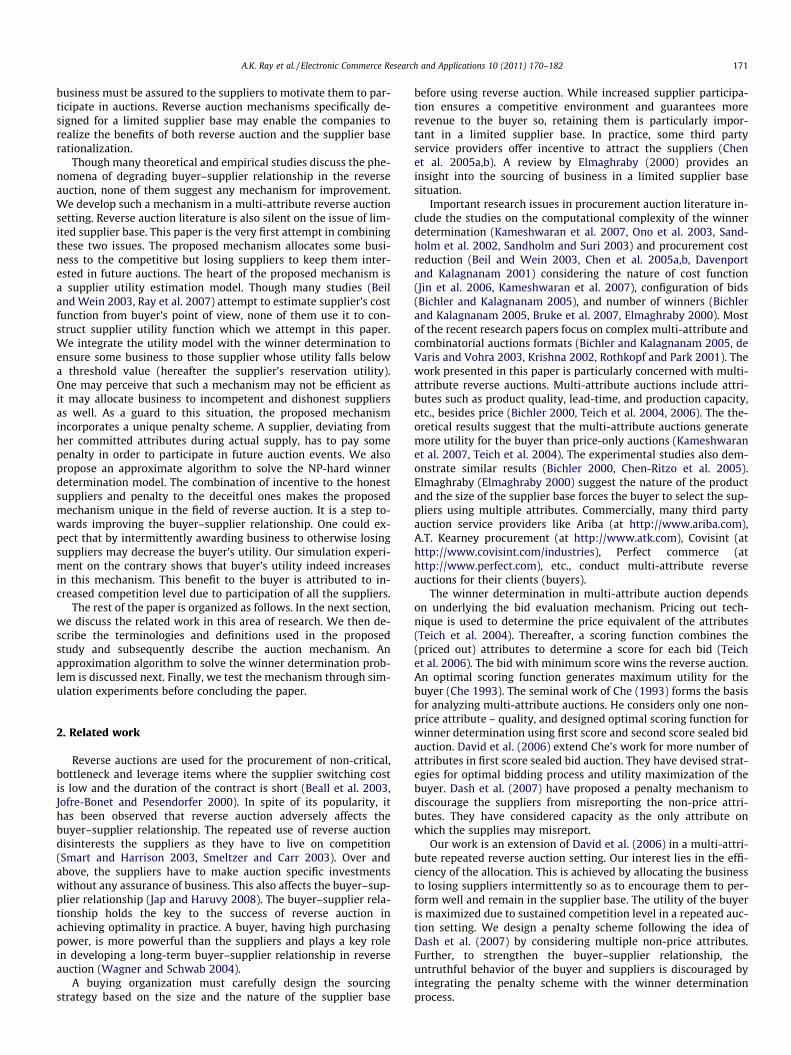
Figs. 3 and 4 show the number of wins and the utility of eachsupplier in Model 2 and Model 1, respectively. It can be observedfrom Figs. 3a and 4a that all the suppliers win in some auctions

Table 5Comparison of the models.

Modeloutput

Numberof samples

Mean St.Dev.

SEmean

95% CI fordifference

Estimate fordifference

p-Value

Model 1 20 1336.7 90.1 20 59.6–145.4 102.5 0.000Model 2 20 1439.2 18.5 4.1

1 2 3 4 5 6 7 8 9 100

1

2

3

4

5

6

7

Supplier ID

Num

ber

of W

ins

(a) Number of wins of the suppliers

Fig. 3. Results of

in Model 2 whereas some of the suppliers do not win at all in Model1. Therefore, the utility of all the suppliers in Model 2 remainsabove their reservation value as shown in Fig. 3b unlike that ofModel 1 where the utilities of 6 suppliers are below the reservationlimit as shown in Fig. 4b.

The results of proposed mechanism are better in two ways: (i)the utility of the buyer is more in comparison to the Model 1 and(ii) the utility of a supplier is above the reservation level. Although,the buyer gives some business to the suppliers who do not getbusiness, the utility of the buyer is not affected because ofcompetition.

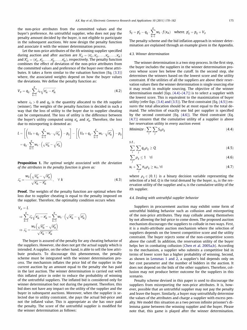
Fig. 5 shows the individual and cumulative utility of the sup-plier (Supplier 7) from 20 consecutive auctions. As discussed ear-lier, a supplier wins either due to lowest score or incentive.Incentive is given only when her cumulative utility falls belowthe reservation value. Fig. 5 explains the two different situationsin which the supplier becomes a winner. It can be observed that,some business is allocated to the supplier as soon as her cumula-tive utility reaches the reservation utility (shown as a straight line)and thus motivate the supplier to participate in future auctionevents. The utility of the supplier is much higher when she winsthe auction with the lowest score than the utility from theincentive.

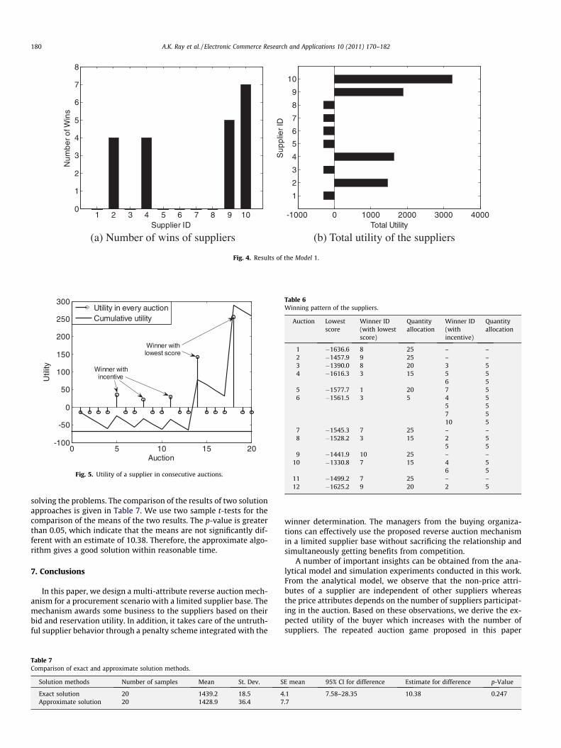
The winning pattern of the suppliers from different auctions isshown in Table 6. It is evident from the table that a supplier whobids with the lowest score becomes the winners in every auction.We call her as a primary winner. In some of the auctions, othersupplier(s) may win due to incentive mechanism. We call themas secondary winners. However, it may be noted that, the amountof business that a secondary winner gets is less in comparison tothe quantity allocated to a primary winner. In fact a secondarywinner will always get the lowest lot size (5 in this case) and theprimary winner will get the remaining demand quantity. There-fore, it is logical for a supplier to win the auction with maximumquantity by bidding as low as possible.

6.4. Comparison of the exact and approximate algorithm

As discussed in Section 5, we have proposed an approximatealgorithm for solving the winner determination problem. Thisalgorithm is implemented in Model 2 in determining the winner(s).For large-size problems, when the number of suppliers as well asthe bids go up, the solution with branch and bound is difficult.We use both (exact and approximate) the solution techniques in

0 200 400 600 800 1000 1200

1

2

3

4

5

6

7

8

9

10

Total Utility

Su

pp

lier

ID

(b) Total utility of the suppliers

the Model 2.

1 2 3 4 5 6 7 8 9 100

1

2

3

4

5

6

7

8

Supplier ID

Num

be

r o

f Win

s

-1000 0 1000 2000 3000 4000

1

2

3

4

5

6

7

8

9

10

Total Utility

Sup

plie

r ID

(a) Number of wins of suppliers (b) Total utility of the suppliers

Fig. 4. Results of the Model 1.

0 5 10 15 20-100

-50

0

50

100

150

200

250

300

Auction

Util

ity

Utility in every auctionCumulative utility

Winner withincentive

Winner withlowest score

Fig. 5. Utility of a supplier in consecutive auctions.

Table 6Winning pattern of the suppliers.

Auction Lowestscore

Winner ID(with lowestscore)

Quantityallocation

Winner ID(withincentive)

Quantityallocation

1 �1636.6 8 25 – –2 �1457.9 9 25 – –3 �1390.0 8 20 3 54 �1616.3 3 15 5 5

6 55 �1577.7 1 20 7 56 �1561.5 3 5 4 5

5 57 510 5

7 �1545.3 7 25 – –8 �1528.2 3 15 2 5

5 59 �1441.9 10 25 – –

10 �1330.8 7 15 4 56 5

11 �1499.2 7 25 – –12 �1625.2 9 20 2 5


solving the problems. The comparison of the results of two solutionapproaches is given in Table 7. We use two sample t-tests for thecomparison of the means of the two results. The p-value is greaterthan 0.05, which indicate that the means are not significantly dif-ferent with an estimate of 10.38. Therefore, the approximate algo-rithm gives a good solution within reasonable time.

7. Conclusions

In this paper, we design a multi-attribute reverse auction mech-anism for a procurement scenario with a limited supplier base. Themechanism awards some business to the suppliers based on theirbid and reservation utility. In addition, it takes care of the untruth-ful supplier behavior through a penalty scheme integrated with the

Table 7Comparison of exact and approximate solution methods.

Solution methods Number of samples Mean St. Dev. S

Exact solution 20 1439.2 18.5 4Approximate solution 20 1428.9 36.4 7

winner determination. The managers from the buying organiza-tions can effectively use the proposed reverse auction mechanismin a limited supplier base without sacrificing the relationship andsimultaneously getting benefits from competition.

A number of important insights can be obtained from the ana-lytical model and simulation experiments conducted in this work.From the analytical model, we observe that the non-price attri-butes of a supplier are independent of other suppliers whereasthe price attributes depends on the number of suppliers participat-ing in the auction. Based on these observations, we derive the ex-pected utility of the buyer which increases with the number ofsuppliers. The repeated auction game proposed in this paper

E mean 95% CI for difference Estimate for difference p-Value

.1 7.58–28.35 10.38 0.247

.7


ensures truthful behavior of both buyer and supplier. We proposeto award some business to the losing but competing suppliers topreserve relationship in a limited supplier base. It appears thatthe buyer may incur some additional cost for preserving therelationship. However, the simulation experiment shows that thebuyer eventually gets benefited from the mechanism because ofthe increased competition level which otherwise would not havehappened with less number of suppliers. The buyer maintains ahealthy competition among the suppliers by retaining them inthe supplier base by preserving their utility. These findings will en-able the buyer to use reverse auction as an efficient procurementtool in a limited supplier base. In addition, it provides new direc-tions to the reverse auction research community.

We are the first to investigate the reverse auction mechanismfrom relationship perspective. This work has many contributions.First, a mechanism that provides incentive to the suppliers in theform of business so as to keep them interested to participate in re-peated auctions. Second, the concept of a penalty scheme, inte-grated with the winner determination model to discourage theuntruthful supplier behavior, makes the mechanism distinct inthe area of auction design. Third, we present a methodology to esti-mate the utility of a supplier by the buyer. In addition, the pro-posed approximate algorithm can be used in online environmentfor fast winner determination.

The results derived and used for the design of the proposedmechanism depend on the nature of the cost function of a supplierand valuation function of the buyer. Any change in the nature ofthe functions will also change the derived expressions. This workcan be extended using various other cost functions and the valua-tion functions. Direct revelation mechanism in multi-attribute re-verse auction may be suitably designed to consider the buyer–supplier relationship. We are currently working towards designingand conducting online experiments with human subjects to studythe effect of the proposed mechanism. New business rules can beadded to the proposed auction mechanism as constraints depend-ing on the complexity of the procurement scenario. Auction mech-anisms such as combinatorial auction can be suitably modified forlimited supplier base in the light of this work.

Table A1The bids and the scores from the suppliers.

Price bidXi1 = {pij, qij}

Non-price bidXi2 = {xi1, xi2}

Scores

qi1 qi2

Supplier 1 (67, 10) (134, 20) (1.6, 2.4) �35.75 �71.51Supplier 2 (154, 10) (308, 20) (6.25, 9.7) �51.72 �103.44Supplier 3 (50, 10) (100, 20) (1, 1.56) �32.35 �64.9

Table A2Utility of the suppliers.

Scores

qi1 qi2

Supplier 1 15.8 31.6Supplier 2 51.4 102.8Supplier 3 8.8 17.6

Acknowledgements

We are thankful to the anonymous reviewers for their invalu-able comments in significantly improving the quality of the paper.We sincerely acknowledge their effort.

Appendix A

A.1. A numerical example

Consider a situation where a company wants to procure 20units of a single item using multi-attribute reverse auction. Theattributes for the selection of the suppliers are price, quality andthe lead-time. Assume all the non-price attributes are in a scaleof 1–10 where 1 represents the lowest and 10 represents the high-est. The lead-time is an inhibiting attribute and we assume a con-version as: converted lead-time = 11 � (lead-time). The bids areaccepted in the lot size of either 10 or 20. For this item, the com-pany has a limited supplier base with three suppliers. We assumeall the suppliers respond to the Request for Quotation and submitmulti-attribute bids. Formally we denote

Suppliers ID: ‘i’, i e {1, 2, 3}Attributes for selection: quality (xi1) and converted lead-time(xi2)Two lots with lot ID ‘j’ j e {1, 2}

We assume that the utility functions of the suppliers followingEq. (3.2) are as follows:

U1j ¼ p1j � qijð0:8 � x11 þ 1:6 � x12ÞU2j ¼ p2j � q2jð0:4 � x21 þ 0:8 � x22ÞU3j ¼ p3j � q3jð1 � x31 þ 2 � x32Þ

Note that, each supplier has a unique cost parameter and accord-ingly decides the bids following Eqs. (3.6) and (3.7), as shown in Ta-ble A1. Each supplier submits two price bids one for each lot(columns 2 and 3) and a non-price bid (column 4).

A.2. The winner determination

In order to determine the winner we find the scores from thesuppliers’ bids. The scoring function (Eq. (3.4)) declared by thebuyer in the beginning of the auction is given as

Sij ¼ pij � qij: 2 �ffiffiffiffiffiffixi1p

þ 5 �ffiffiffiffiffiffixi2p

ð Þ

The scores for every bid of each supplier are shown in Table 7, col-umns 5 and 6. The supplier with the lowest score wins the auction.Note that lowest score indicates lower price and higher non-priceattribute values and is aligned with the objective of the buyer. Inthis case, Supplier 2 having a score of �103.44 wins the auction.

The expression for the utility of the buyer is Ub ¼ 100þqij � 2 � ffiffiffiffiffiffi

xi1p þ 5 � ffiffiffiffiffiffi

xi2pð Þ � pij (Eq. (3.5)). Therefore, utility of the

buyer from the winning bid is equal to Ub = 203.44. Suppliers’ util-ities calculated from different bids are given in Table A2. The utilityof the winning supplier is shown in bold face.

A.3. Integration of the penalty mechanism with the winnerdetermination

In the above example, the Supplier 2 is the winner and suppliesthe product according to the contract terms. However, after the ac-tual supply, the buyer determines the non-price attributes (qualityand lead-time) to be (5.25, 6.7) instead of (6.25, 9.7) as promisedduring auction (Table A1). The buyer now charges a penaltyaccording to the following function (Eq. (4.2))

Vp ¼ 20 0:3 �ffiffiffiffiffiffiffiffiffiffiffiffiffiffiffiffiffix�ik � xc

ik

qþ 1:53 �


ik

q� �The penalty amount (here 61.48) is to be paid by Supplier 2 to thebuyer. If the supplier does not pay then she is not allowed to partic-ipate in the subsequent auctions. To continue with the example as-sume that the supplier pays the fine and participates in the next

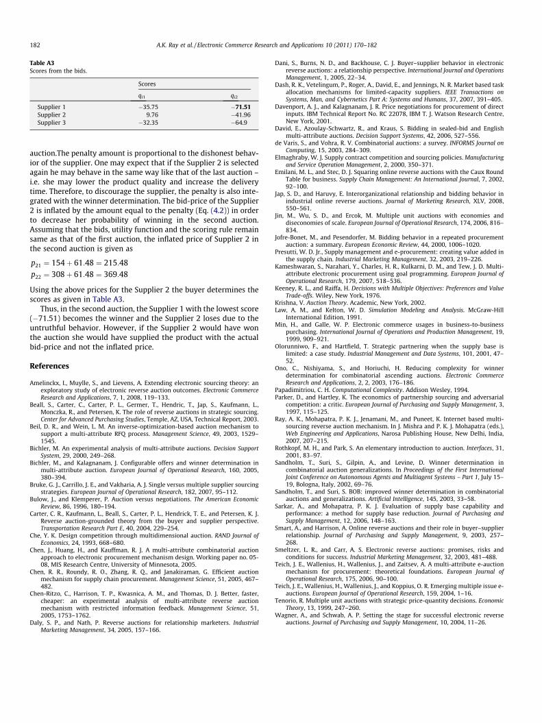
Table A3Scores from the bids.

Scores

qi1 qi2

Supplier 1 �35.75 �71.51Supplier 2 9.76 �41.96Supplier 3 �32.35 �64.9


auction.The penalty amount is proportional to the dishonest behav-ior of the supplier. One may expect that if the Supplier 2 is selectedagain he may behave in the same way like that of the last auction –i.e. she may lower the product quality and increase the deliverytime. Therefore, to discourage the supplier, the penalty is also inte-grated with the winner determination. The bid-price of the Supplier2 is inflated by the amount equal to the penalty (Eq. (4.2)) in orderto decrease her probability of winning in the second auction.Assuming that the bids, utility function and the scoring rule remainsame as that of the first auction, the inflated price of Supplier 2 inthe second auction is given as

p21 ¼ 154þ 61:48 ¼ 215:48p22 ¼ 308þ 61:48 ¼ 369:48

Using the above prices for the Supplier 2 the buyer determines thescores as given in Table A3.

Thus, in the second auction, the Supplier 1 with the lowest score(�71.51) becomes the winner and the Supplier 2 loses due to theuntruthful behavior. However, if the Supplier 2 would have wonthe auction she would have supplied the product with the actualbid-price and not the inflated price.

References

Amelinckx, I., Muylle, S., and Lievens, A. Extending electronic sourcing theory: anexploratory study of electronic reverse auction outcomes. Electronic CommerceResearch and Applications, 7, 1, 2008, 119–133.

Beall, S., Carter, C., Carter, P. L., Germer, T., Hendric, T., Jap, S., Kaufmann, L.,Monczka, R., and Petersen, K. The role of reverse auctions in strategic sourcing.Center for Advanced Purchasing Studies, Temple, AZ, USA, Technical Report, 2003.

Beil, D. R., and Wein, L. M. An inverse-optimization-based auction mechanism tosupport a multi-attribute RFQ process. Management Science, 49, 2003, 1529–1545.

Bichler, M. An experimental analysis of multi-attribute auctions. Decision SupportSystem, 29, 2000, 249–268.

Bichler, M., and Kalagnanam, J. Configurable offers and winner determination inmulti-attribute auction. European Journal of Operational Research, 160, 2005,380–394.

Bruke, G. J., Carrillo, J. E., and Vakharia, A. J. Single versus multiple supplier sourcingstrategies. European Journal of Operational Research, 182, 2007, 95–112.

Bulow, J., and Klemperer, P. Auction versus negotiations. The American EconomicReview, 86, 1996, 180–194.

Carter, C. R., Kaufmann, L., Beall, S., Carter, P. L., Hendrick, T. E., and Petersen, K. J.Reverse auction-grounded theory from the buyer and supplier perspective.Transportation Research Part E, 40, 2004, 229–254.

Che, Y. K. Design competition through multidimensional auction. RAND Journal ofEconomics, 24, 1993, 668–680.

Chen, J., Huang, H., and Kauffman, R. J. A multi-attribute combinatorial auctionapproach to electronic procurement mechanism design. Working paper no. 05-08, MIS Research Centre, University of Minnesota, 2005.

Chen, R. R., Roundy, R. O., Zhang, R. Q., and Janakiraman, G. Efficient auctionmechanism for supply chain procurement. Management Science, 51, 2005, 467–482.

Chen-Ritzo, C., Harrison, T. P., Kwasnica, A. M., and Thomas, D. J. Better, faster,cheaper: an experimental analysis of multi-attribute reverse auctionmechanism with restricted information feedback. Management Science, 51,2005, 1753–1762.

Daly, S. P., and Nath, P. Reverse auctions for relationship marketers. IndustrialMarketing Management, 34, 2005, 157–166.

Dani, S., Burns, N. D., and Backhouse, C. J. Buyer–supplier behavior in electronicreverse auctions: a relationship perspective. International Journal and OperationsManagement, 1, 2005, 22–34.

Dash, R. K., Vetelingum, P., Roger, A., David, E., and Jennings, N. R. Market based taskallocation mechanisms for limited-capacity suppliers. IEEE Transactions onSystems, Man, and Cybernetics Part A: Systems and Humans, 37, 2007, 391–405.

Davenport, A. J., and Kalagnanam, J. R. Price negotiations for procurement of directinputs. IBM Technical Report No. RC 22078, IBM T. J. Watson Research Centre,New York, 2001.

David, E., Azoulay-Schwartz, R., and Kraus, S. Bidding in sealed-bid and Englishmulti-attribute auctions. Decision Support Systems, 42, 2006, 527–556.

de Varis, S., and Vohra, R. V. Combinatorial auctions: a survey. INFORMS Journal onComputing, 15, 2003, 284–309.

Elmaghraby, W. J. Supply contract competition and sourcing policies. Manufacturingand Service Operation Management, 2, 2000, 350–371.

Emilani, M. L., and Stec, D. J. Squaring online reverse auctions with the Caux RoundTable for business. Supply Chain Management: An International Journal, 7, 2002,92–100.

Jap, S. D., and Haruvy, E. Interorganizational relationship and bidding behavior inindustrial online reverse auctions. Journal of Marketing Research, XLV, 2008,550–561.

Jin, M., Wu, S. D., and Ercok, M. Multiple unit auctions with economies anddiseconomies of scale. European Journal of Operational Research, 174, 2006, 816–834.

Jofre-Bonet, M., and Pesendorfer, M. Bidding behavior in a repeated procurementauction: a summary. European Economic Review, 44, 2000, 1006–1020.

Presutti, W. D. Jr., Supply management and e-procurement: creating value added inthe supply chain. Industrial Marketing Management, 32, 2003, 219–226.

Kameshwaran, S., Narahari, Y., Charles, H. R., Kulkarni, D. M., and Tew, J. D. Multi-attribute electronic procurement using goal programming. European Journal ofOperational Research, 179, 2007, 518–536.

Keeney, R. L., and Raiffa, H. Decisions with Multiple Objectives: Preferences and ValueTrade-offs. Wiley, New York, 1976.

Krishna, V. Auction Theory. Academic, New York, 2002.Law, A. M., and Kelton, W. D. Simulation Modeling and Analysis. McGraw-Hill

International Edition, 1991.Min, H., and Galle, W. P. Electronic commerce usages in business-to-business

purchasing. International Journal of Operations and Production Management, 19,1999, 909–921.

Olorunniwo, F., and Hartfield, T. Strategic partnering when the supply base islimited: a case study. Industrial Management and Data Systems, 101, 2001, 47–52.

Ono, C., Nishiyama, S., and Horiuchi, H. Reducing complexity for winnerdetermination for combinatorial ascending auctions. Electronic CommerceResearch and Applications, 2, 2, 2003, 176–186.

Papadimitriou, C. H. Computational Complexity. Addison Wesley, 1994.Parker, D., and Hartley, K. The economics of partnership sourcing and adversarial

competition: a critic. European Journal of Purchasing and Supply Management, 3,1997, 115–125.

Ray, A. K., Mohapatra, P. K. J., Jenamani, M., and Puneet, K. Internet based multi-sourcing reverse auction mechanism. In J. Mishra and P. K. J. Mohapatra (eds.),Web Engineering and Applications, Narosa Publishing House, New Delhi, India,2007, 207–215.

Rothkopf, M. H., and Park, S. An elementary introduction to auction. Interfaces, 31,2001, 83–97.

Sandholm, T., Suri, S., Gilpin, A., and Levine, D. Winner determination incombinatorial auction generalizations. In Proceedings of the First InternationalJoint Conference on Autonomous Agents and Multiagent Systems – Part 1, July 15–19, Bologna, Italy, 2002, 69–76.

Sandholm, T., and Suri, S. BOB: improved winner determination in combinatorialauctions and generalizations. Artificial Intelligence, 145, 2003, 33–58.

Sarkar, A., and Mohapatra, P. K. J. Evaluation of supply base capability andperformance: a method for supply base reduction. Journal of Purchasing andSupply Management, 12, 2006, 148–163.

Smart, A., and Harrison, A. Online reverse auctions and their role in buyer–supplierrelationship. Journal of Purchasing and Supply Management, 9, 2003, 257–268.

Smeltzer, L. R., and Carr, A. S. Electronic reverse auctions: promises, risks andconditions for success. Industrial Marketing Management, 32, 2003, 481–488.

Teich, J. E., Wallenius, H., Wallenius, J., and Zaitsev, A. A multi-attribute e-auctionmechanism for procurement: theoretical foundations. European Journal ofOperational Research, 175, 2006, 90–100.

Teich, J. E., Wallenius, H., Wallenius, J., and Koppius, O. R. Emerging multiple issue e-auctions. European Journal of Operational Research, 159, 2004, 1–16.

Tenorio, R. Multiple unit auctions with strategic price-quantity decisions. EconomicTheory, 13, 1999, 247–260.

Wagner, A., and Schwab, A. P. Setting the stage for successful electronic reverseauctions. Journal of Purchasing and Supply Management, 10, 2004, 11–26.

an efficient reverse auction mechanism for limited supplier base

Documents