an approach to on-line identification of takagi-sugeno...

484 IEEE TRANSACTIONS ON SYSTEMS, MAN, AND CYBERNETICS—PART B: CYBERNETICS, VOL. 34, NO. 1, FEBRUARY 2004

An Approach to Online Identification ofTakagi-Sugeno Fuzzy Models

Plamen P. Angelov, Member, IEEE, and Dimitar P. Filev, Senior Member, IEEE

Abstract—An approach to the online learning of Takagi–Sugeno(TS) type models is proposed in the paper. It is based on a novellearning algorithm that recursively updates TS model structureand parameters by combining supervised and unsupervisedlearning. The rule-base and parameters of the TS model con-tinually evolve by adding new rules with more summarizationpower and by modifying existing rules and parameters. In thisway, the rule-base structure is inherited and up-dated whennew data become available. By applying this learning conceptto the TS model we arrive at a new type adaptive model calledthe Evolving Takagi–Sugeno model (ETS). The adaptive natureof these evolving TS models in combination with the highlytransparent and compact form of fuzzy rules makes them apromising candidate for online modeling and control of complexprocesses, competitive to neural networks. The approach has beentested on data from an air-conditioning installation serving a realbuilding. The results illustrate the viability and efficiency of theapproach. The proposed concept, however, has significantly widerimplications in a number of fields, including adaptive nonlinearcontrol, fault detection and diagnostics, performance analysis,forecasting, knowledge extraction, robotics, behavior modeling.

Index Terms—Online recursive identification, rule-base adapta-tion, Takagi–Sugeno models.

I. INTRODUCTION

TAKAGI–SUGENO models have recently become a pow-erful practical engineering tool for modeling and control

of complex systems. They form a natural transition betweenconventional and rule-based control by expanding and gener-alizing the well-known concept of gain scheduling. While thegain-scheduling [24] paradigm is based on the assumption oflocal approximation of a nonlinear system by a collection oflinear models, the TS models utilize the idea of linearization ina fuzzily defined region of the state space. Due to the fuzzy re-gions, the nonlinear system is decomposed into a multi-modelstructure consisting of linear models that are not necessarily in-dependent [4].

The TS model representation often provides efficient andcomputationally attractive solutions to a wide range of controlproblems introducing a powerful multiple model structure thatis capable to approximate nonlinear dynamics, multiple oper-ating modes and significant parameter and structure variations.

Manuscript received May 24, 2002; revised December 5, 2002. This workused data generated from the ASHRAE Project RP1020. This paper was rec-ommended by Associate Editor L. O. Hall.

P. P. Angelov is with the Department of Communications Systems, LancasterUniversity, Bailrigg, Lancaster LA1 4YR, U.K. (e-mail: [email protected]).

D. P. Filev is with the Ford Motor Co., Detroit, MI 48239 USA (e-mail:[email protected]).

Digital Object Identifier 10.1109/TSMCB.2003.817053

The methods for learning TS models from data are based onthe idea of consecutive structure and parameter identification[3], [14]. Structure identification includes estimation of the focalpoints of the rules (antecedent parameters) by fuzzy clustering.With fixed antecedent parameters, the TS model transforms intoa linear model. Parameters of the linear models associated witheach of the rule antecedents are obtained by pseudo-inversionor by applying the recursive least square (RLS) method [16],[28]. Alternatively, the antecedent parameters can be consid-ered as initial estimates only and the structure and parameterscan be further optimized by back-propagation [20] or geneticalgorithm [12]. These methods, however, suppose that all thedata is available at the start of the process of training. There-fore, they are appropriate for offline applications only. Their usein online algorithms is only possible for the price of re-trainingthe whole model structure and parameters with iterative andtime-consuming procedures such as back-propagation [5], ge-netic algorithms [6]–[8], [10]–[12] or other nonlinear searchtechniques [1], [21], [29].

Although some objects, including biotechnological pro-cesses, building thermal systems, etc. have relatively slowdynamics, making such re-training possible, it is difficult tocharacterize it as adaptation, especially in respect to the modelstructure. It is in fact, a procedure where completely newmodels are repeatedly generated given the new data. The factthat fuzzy models are still not adaptive, while in many practicalproblems the control object or the environment is changingsignificantly is an important obstacle in their design, which isstill unresolved [19].

For continuous online learning of the TS models a develop-ment of a new online clustering method responsible for modelstructure (rule base) learning online is needed. This requires re-cursive calculation of the informative potential of the data [9],which represents a spatial proximity measure used to define thefocal points of the rules (antecedent parameters). If suppose thatthe model structure evolves similarly to the model parameters,though much slower, then we need suitable new algorithms foronline clustering and recursive parameter estimation with thisassumption. The purpose of this paper is to present such algo-rithms and the results of their application to a number of testcases both simulated and real.

Recently, rule-bases [9], [15], [27] and neural networks [20],[31] with evolving structure have been developed. Rule-base ofInitial Conditions, RBIC [15], Intelligent Model Bank [27] andthe Self-constructing fuzzy-neural network controller [20] areprimarily oriented to control applications. They use differentmechanism of rules update based on the distance to certainrule center [15], [27], [31] or the error in previous steps [20].

1083-4419/04$20.00 © 2004 IEEE

ANGELOV AND FILEV: APPROACH TO ONLINE IDENTIFICATION 485

Evolving rule-based models [9] use the informative po-tential of the new data sample (accumulated spatial proximityinformation) as a trigger to update the rule-base, which ensuresgreater generality of the structural changes. Outliers have nochance to become rule centers. It also ensures that the rules aremore general (that they are able to describe a larger number ofdata samples) from time of their initialization. In addition, themechanism of rule-base modification (replacement of a lessinformative rule with a more informative one) is consideredin [9]. It is also based on the informative potential and ismore conservative than the replacement used in [15], [27],[31] ensuring a gradual change of the rule-base structure andinheritance of the structural information. models generatea new rule if there is significant new information present inthe data collected. The evolution mechanism takes care ofthe replacement of existing rules based on the accumulatedmeasure of the spatial proximity of all the data samples. If theinformative potential of the new data sample is higher than theaverage potential of the existing rules it is added to the rulebase. If the new data, which is accepted as a focal point of anew rule is too close to a previously existing rule then the oldrule is replaced by the new one.

The appearance of a new rule indicates a region of the dataspace that has not been covered by the initial training data. Thiscould be a new operating mode of the plant or reaction to a newdisturbance. In reality, many regimes and process states cannotbe practically included into the training data set (such as faultyprocess behavior), but states close to them could well appearduring the process run [22].

It is important to note that learning could start without a prioriinformation and only one data sample. This interesting featuremakes the approach potentially very useful in adaptive control,robotic, diagnostic systems and as a tool for knowledge acqui-sition from data.

The concept of modeling [9] is further developed here inrespect to online identification of ETS models. Recursive pro-cedures for calculation of the informative potential of the newdata and of the consequence parameters are introduced, whichremove the need of the time moving window considered in [9].This feature is vitally important for real-time applications.

The rest of the paper is organized as follows. The problemof identification of TS models is presented in Section II. Twoalternative ways (globally and locally optimal) of calculation ofthe consequent parameters are presented. The new approach foronline learning ETS models is presented in the next Section III.In Section IV the essential stages of the procedure are definedand systematically described. Section V studies experimentalresults considering a real air-conditioning engineering problem.Concluding remarks are given in Section VI.

II. TS FUZZY MODEL AND THE PROBLEM OF ITS

IDENTIFICATION

Fuzzy model identification has its roots in the pioneering pa-pers of Sugeno and his coworkers [13], [14] and is associatedwith the so-called Takagi-Sugeno (TS) fuzzy models—a specialgroup of rule-based models with fuzzy antecedents and func-

tional consequents that follow from the Takagi–Sugeno–Kangreasoning method:

(1)

where denotes the fuzzy rule; is the number of fuzzyrules; is the input vector; ; denotesthe antecedent fuzzy sets, ; is the output of thelinear subsystem; are its parameters, .

The TS model paradigm [13] can be considered as a gener-alization of the gain-scheduling concept. Instead of linearizingstrictly at an operating point it utilizes the idea of linearizationin a fuzzily defined region of the space. The fuzzy regions areparameterized and each region is associated with a linear sub-system. Owing to the fuzzily defined antecedents, the nonlinearsystem forms a collection of loosely coupled multiple linearmodels. The degree of firing of each rule is proportional to thelevel of contribution of the corresponding linear model to theoverall output of the TS model. For Gaussian-like antecedentfuzzy sets

(2)

where and is a positive constant, which defines thespread of the antecedent and the zone of influence of themodel (radius of the neighborhood of a data point); too large avalue of leads to averaging, too small a value—to over-fitting;values of can be recommended ) [16]; is thefocal point of the rule antecedent.

The firing level of the rules are defined as Cartesian productor conjunction of respective fuzzy sets for this rule

(3)

The TS model output is calculated by weighted averaging ofindividual rules’ contributions

(4)

where is the normalized firing level of therule; represents the output of the linear model;

, , is the vector of parameters ofthe linear model; is the expanded data vector.

Generally, the problem of identification of a TS model is di-vided into two sub-tasks [3], [13], [16].

i) Learning the antecedent part of the model (1), which con-sists of determination of the focal points of the rules, i.e.,the centers ( ; ) and spreads of the mem-bership functions.

ii) Learning the parameters of the linear subsystems ( ;; ) of the consequents.

A. Learning Rule Antecedents by Data Space Clustering

First sub-task can be solved by clustering the input-outputdata space . The Subtractive Clustering method[16], Fuzzy C-means [17], and the Gustafson–Kessel clustering


method [23] are among the well-established methods forlearning the antecedent parameters offline in a batch-processinglearning mode when all the input-output data is available.

The procedure called subtractive clustering [16] is an im-proved version of the so-called mountain clustering approach[25]. It uses the data points as candidate prototype cluster cen-ters. The capability of a point to be a cluster center is evaluatedthrough its potential—a measure of the spatial proximity be-tween a particular point and all other data points

(5)

where denote the potential of the data point and whereis the number of training data).

As seen from (5) the value of the potential is higher for adata point that is surrounded by a large number of close datapoints. Therefore, it is reasonable to establish such a point tobe the center of a cluster [24]. The potential of all other datapoints is reduced by an amount proportional to the potential ofthe chosen point and inversely proportional to the distance tothis center. The next center is found also as the data point withthe highest (after this subtraction) potential. The procedure isrepeated until the potential of all data points is reduced below acertain threshold.

The procedure of the subtractive clustering includes the fol-lowing steps [16].

1) Initially, the data point with the highest potential is chosento be the first cluster center

(6)

where denotes the potential of the first center.2) The potential of all other points are then reduced by an

amount proportional to the potential of the chosen pointand inversely proportional to the distance to this center

(7)

where denotes the potential of the center;; ; where is a positive constant,

determining the radius of the neighborhood that willhave measurable reductions in the potential because ofthe closeness to an existing center; recommended valueof is [16].

3) Two boundary conditions are defined: lowerand upper threshold, determined as a functionof the maximal potential called the “reference” potential

. A data point is chosen to be a new cluster center,and respectively center of a rule, if its potential is higherthan the upper threshold.

4) If the potential of a point lies between the two boundaries,the shortest of the distances between the new can-didate to be a cluster center and all previously found

cluster centers is decisive. The following inequality, ex-press the trade-off between the potential value and thecloseness to the previous centers

(8)

This approach has been used for initial estimation of the an-tecedent parameters in fuzzy identification. It relies on the ideathat each cluster center is representative of a characteristic be-havior of the system [16]. The resulting cluster centers are usedas parameters of the antecedent parts defining the focal pointsof the rules of the model.

B. Learning Parameters of Linear Subsystems

For fixed antecedent parameters the second sub-task, estima-tion of the parameters of the consequent linear models can betransformed into a least squared problem [2]. This is accom-plished by eliminating the summation operation in (4) and re-placing it with an equivalent vector expression of

(9)

where is a vector composed of the linearmodel parameters; is a vectorof the inputs that are weighted by the normalized firing levelsof the rules.

For a given set of input-output data , ,the vector of linear model parameters minimizing the objectivefunction is

(10)

where ;, can be estimated by the recursive least squares algo-

rithm (called also the Kalman filter) [13], [16]

(11)

(12)

with initial conditions and , where is a largepositive number; C is a co-variance matrix;

is an estimation of the parameters based on data samples.Alternatively, the objective function (10) can be written in

vector form as

(10a)

where the matrix and vector Y are formed by , and ,.

Then the vector minimizing (10a) could be obtained by thepseudo-inversion

(13)

The objective functions (10), (10a) are globally optimal, but thisdoes not guarantee locally adequate behavior of the sub-modelsthat form the TS model [18]. Locally meaningful sub-models


could be found using the locally weighted objective function[18], [28]

(14)

where matrix X is formed by ; ; matrixis a diagonal matrix with as its elements in the main

diagonal.An approximate solution minimizing the cost function (14)

can be obtained by assuming the linear subsystems are looselycoupled with levels of interaction expressed by the weights

. Then (14) can be regarded as a sum of cost functions

where

(15)

The solutions that minimize the weighted least square prob-lems expressed by the objective functions can be obtainedby applying a weighted pseudo-inversion [18], [28]

(16)

Alternatively, a set of solutions to individual cost functions(vectors ’s) can be recursively calculated through the

weighted RLS (wRLS) algorithm. In this case, a wRLS algo-rithm that minimizes each of the cost functions is appliedto the linear subsystem associated with each rule (see theAppendix for the detailed derivation)

(17)

(18)

with initial conditions and .As seen from (17), (18) when the normalized firing weight

of certain rule is equal to 1 the wRLS algorithm transformsinto RLS (11), (12) based on this rule only . For therule for which the normalized firing level is 0 for a certaintime step the parameters and the co-variancematrix stay unchanged ( ; ). When

the update of the co-variance matrix and parametersare weighted by the normalized firing level.

III. ONLINE LEARNING OF TS MODELS

In Online mode, the training data are collected continuously,rather than being a fixed set. Some of the new data reinforce andconfirm the information contained in the previous data. Otherdata, however, bring new information, which could indicate achange in operating conditions, development of a fault or simplya more significant change in the dynamic of the process [9].

They may posses enough new information to form a new ruleor to modify an existing one. The value of the information theybring is closely related to the information the data collected sofar already possesses. The judgement of the informative poten-tial and importance of the data is made based on their spatialproximity, which corresponds to operating conditions, possiblyseasonal variations or different faults.

online learning of ETS models includes online clusteringunder assumption of a gradual change of the rule-base andmodified (weighted) recursive least squares. Due to the evo-lution of the model structure, the number of fuzzy rules isexpected to grow. This is, however, significantly slower thanthe growth of the size of the data vectors, because the potentialis inversely proportional to the number of the data points (5).

A. Online Clustering Approach

The online clustering procedure starts with the first data pointestablished as the focal point of the first cluster. Its coordinatesare used to form the antecedent part of the fuzzy rule (1) usingfor example Gaussian membership functions (2). Any other typeof membership functions could also be used instead. Its potentialis assumed equal to 1.

Starting from the next data point onwards the potential of thenew data points is calculated recursively. As a measure of thepotential, we use a Cauchy type function of first order

(19)where denotes the potential of the data point cal-culated at time ; , denotes projection of the dis-tance between two data points ( and ) on the axis ( for

and on the axis for ).This function is monotonic and inversely proportional to the

distance and enables recursive calculation, which is importantfor online implementation of the learning algorithm. Addition-ally, we do not subtract a specified amount from the highest po-tential, but update all the potentials after a new data point isavailable online.

Potential of the new data sample is recursively calculated asfollows (see the Appendix for details)

(20)

where ; ;

; .Parameters and in (20) are calculated from the current

data point , while and are recursively updated as; .

After the new data are available in online mode, they influ-ence the potentials of the centers of the clusters ( , ),which are respective to the focal points of the existing rules( , ). The reason is that by definition the potentialdepends on the distance to all data points, including the newones (the sum in the denominator by in (19) has an increasingnumber of components). The recursive formula for update of the


potentials of the focal points of the existing clusters can easilybe derived from (19) (see the Appendix for details)

(21)where is the potential at time of the cluster center,which is a prototype of the rule. Potentials of the new datapoints are compared to the updated potential of the centers ofthe existing clusters.

If the potential of the new data point is higher than the poten-tial of the existing centers then the new data point is accepted asa new center and a new rule is formed with a focal point basedon the projection of this center on the axis ( ;

). The rationale is that in this case the new data pointis more descriptive, has more summarization power than all theother data points. It should be noted that the condition to havehigher potential is a very strong one. The reason is that withthe growing number of data, their concentration is usually de-creasing except in the cases some new important region of dataspace reflecting a new operating regime [4] or new conditionappears. In such cases a new rule is formed, while outlying dataare automatically rejected because their potential is significantlylower due to their distance from the other data. This propertyof the proposed approach is very promising for fault detectionproblems.

If in addition to the previous condition (the potential of thenew data point is higher that the potential of all the previouslyexisting centers) the new data point is close to an old center

(22)

then the new data point replaces this center .This mechanism for rule-base adaptation called modification en-sures a replacement of a rule with another one built around theprojection of the new data point on the axis .

It should be noted that using the potential instead of the dis-tance to a certain rule center only [15], [27], [31] for forming therule-base results in rules that are more informative and a morecompact rule-base. The reason is that the spatial information andhistory are not ignored, but are part of the decision whether toupgrade or modify the rule-base.

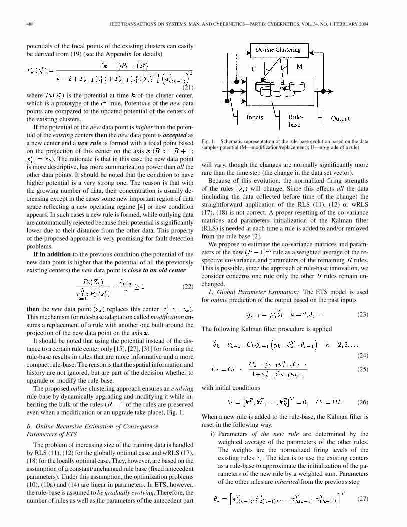
The proposed online clustering approach ensures an evolvingrule-base by dynamically upgrading and modifying it while in-heriting the bulk of the rules ( of the rules are preservedeven when a modification or an upgrade take place), Fig. 1.

B. Online Recursive Estimation of ConsequenceParameters of ETS

The problem of increasing size of the training data is handledby RLS (11), (12) for the globally optimal case and wRLS (17),(18) for the locally optimal case. They, however, are based on theassumption of a constant/unchanged rule base (fixed antecedentparameters). Under this assumption, the optimization problems(10), (10a) and (14) are linear in parameters. In ETS, however,the rule-base is assumed to be gradually evolving. Therefore, thenumber of rules as well as the parameters of the antecedent part

Fig. 1. Schematic representation of the rule-base evolution based on the datasamples potential (M—modification/replacement); U—up-grade of a rule).

will vary, though the changes are normally significantly morerare than the time step (the change in the data set vector).

Because of this evolution, the normalized firing strengthsof the rules will change. Since this effects all the data(including the data collected before time of the change) thestraightforward application of the RLS (11), (12) or wRLS(17), (18) is not correct. A proper resetting of the co-variancematrices and parameters initialization of the Kalman filter(RLS) is needed at each time a rule is added to and/or removedfrom the rule base [2].

We propose to estimate the co-variance matrices and param-eters of the new rule as a weighted average of the re-spective co-variance and parameters of the remaining rules.This is possible, since the approach of rule-base innovation, weconsider concerns one rule only the other rules remain un-changed.

1) Global Parameter Estimation: The ETS model is usedfor online prediction of the output based on the past inputs

(23)

The following Kalman filter procedure is applied

(24)

(25)

with initial conditions

(26)

When a new rule is added to the rule-base, the Kalman filter isreset in the following way.

i) Parameters of the new rule are determined by theweighted average of the parameters of the other rules.The weights are the normalized firing levels of theexisting rules . The idea is to use the existing centersas a rule-base to approximate the initialization of the pa-rameters of the new rule by a weighted sum. Parametersof the other rules are inherited from the previous step

(27)


where

(27a)

ii) Co-variance matrices are reset as

(28)where is an element of the co-variance matrix (

; );is a coefficient.

In this way, the part of the co-variance matrix associated withthe new rule (last columns and last rows)is initialized as usual (with a large number in its main di-agonal and co-variance matrices respective for the rest of therules (from 1 to ) are updated by multiplication of (28). Therationale for this is that the correction the co-variance matricesneeds, to approximate the role the new, rule wouldhave if it was in the rule-base from the beginning, can be repre-sented by (see the Appendix).

When a rule is replaced by another one, which has antecedentparameter close to the rule being replaced, then parameters andco-variance matrices are inherited from the previous time step.

2) Local Parameter Estimation: The local parameter esti-mation is based on the wRLS

(29)

(30)

with initial conditions

(31)

In this case, the co-variance matrices are separate for eachrule and have smaller dimensions ( ;

). Parameters of the newly added rule are determined asweighted average of the parameters of the rest rules by (27a).Parameters of the other rules are inherited ( ;

).When a rule is replaced by another rule, which have close

antecedent parameter (center) then parameters of all rules areinherited ( ; ).

The co-variance matrix of the newly added rule is initializedby

(32)

The co-variance matrices of the rest rules are inherited (; ).

IV. PROCEDURE FOR RULE-BASE EVOLUTION IN ETS MODELS

The recursive procedure for online learning of ETS models,introduced in this paper, includes the following stages.

1) Stage 1: Initialization of the rule-base structure (an-tecedent part of the rules).

2) Stage 2: At the next time step reading the next datasample.

3) Stage 3: Recursive calculation of the potential of each newdata sample to influence the structure of the rule-base.

4) Stage 4: Recursive up-date of the potentials of old centerstaking into account the influence of the new data sample.

5) Stage 5: Possible modification or up-grade of therule-base structure based on the potential of the new datasample in comparison to the potential of the existingrules’ centers (focal points).

6) Stage 6: Recursive calculation of the consequent param-eters.

7) Stage 7: Prediction of the output for the next time step bythe ETS model.

The execution of the algorithm continues for the next time stepfrom stage 2. It should be noted that the first output to be pre-dicted is .

Stage 1. The rule-base could contain one single rule only,based, for example, on the first data sample. Then

(33)

where is the first cluster center; is focal point of the firstrule being a projection of on the axis .

In principle, the rule-base could be initialized by existing ex-pert knowledge. Generally, however, it could be based on theoff-line identification approaches, described in Section II. In thiscase

(34)

where denotes the number of rules defined initially off-line.Stages 2 to 7 are performed online. They form the distinctive

characteristics of the proposed approach.Stage 2. At the next time step the new data

sample is collected.At stage 3 the potential of each new data sample is recursively

calculated by (20). The use of already calculated values andleads to significant time and calculation savings because

(19) is normally calculated from large matrices (the number oftraining data in online mode is continuously growing). At thesame time, they have accumulated information regarding thespatial proximity of all previous data.

At stage 4 the potentials of the focal points (centers) of theexisting clusters/rules are recursively updated by (21).

At stage 5 the potential of the new data sample is compared tothe updated potential of existing centers and a decision whetherto modify or up-grade the rule-base is taken.

a)

IF (the potential new data pointis higher than the potential of the


existing centers: ;)

AND [the new data point is close toan old center (22)]THEN the new data point re-places it.

In this case, the new data point is used as a prototype ofa focal point (let us suppose that it has index

(35)Consequence parameters and co-variance matrices are in-herited from the rule to be replaced

(36)

It should be noted that when a rule is replaced by anotherrule the weights are changing according to (4) andthe summation in the denominator in (4) should change.

addends in this summation are the same and onlyone change. Moreover, since the new center is close to thereplaced one by definition (22), this change is marginal.The disturbance caused to the RLS by this change couldbe ignored, because the Kalman filter is able to cope withthis disturbance starting from the existing estimations ofthe parameters and co-variance matrices. This is also illus-trated by the experimental results (next section).

b)

ELSE IF (the potential of the newdata point is higher than the po-tential of the existing centers:

; )THEN it is added to the rule-baseas a new rule’s center.

In this case, the new data point becomes a prototype ofa focal point of a new rule

(37)

Consequence parameters and co-variance matrices arereset by (27)–(28) or (32), respectively, for the global orlocal estimation.

END IF

At Stage 6 parameters of the consequence are recursively up-dated by RLS (24), (25) with initializations (26) for globally op-timal parameters or by wRLS (29), (30) with initializations (31)for locally optimal parameters.

In the first case the cost function (10) is minimized, whichguarantees globally optimal values of the parameters, while inthe second case the locally weighted cost function (15) is mini-mized and locally meaningful parameters are obtained.

At Stage 7 the output for the next time step is predictedby (23).

The algorithm continues from stage 2 by reading the next datasample at the next time step.

Fig. 2. Block-diagram of the online identification of ETS models.

A graphical representation of the algorithm that realizes theproposed approach is demonstrated in Fig. 2. All steps are non-iterative.

Using the approach, a transparent, compact and accuratemodel can be found by rule base evolution based on experi-mental data with the simultaneous recursive estimation of thefuzzy set parameters. It is interesting to note that the rate ofupgrade with new rules does not lead to an excessively largerule base in comparison to [15], [20], [27], [31]. The reasonfor this is that the condition for the new data point to havehigher potential (19), (20) than the focal points of rules of allexisting rules is a hard requirement. Additionally, the possibleproximity of a candidate center to the already existing focalpoints leads to just a replacement of the existing focal point, i.e.modification of its coordinates without enlarging the rule-basesize.

V. EXPERIMENTAL RESULTS

The new algorithm has been tested on the data from afan-coil sub-system of an air-conditioning system serving a realbuilding. Training data were collected on August 3, and August19, 1998 (courtesy of ASHRAE for the use of data, generatedfrom the ASHRAE funded research project RP1020).


Fig. 3. Experimental set-up.

Fig. 4. Absolute error in prediction the valve position using global parameterestimation.

The ETS model of the position of the valve controllingthe water flow rate to a fan-coil sub-system has been consid-ered (Fig. 3). The model makes online prediction of the valveposition steps ahead (the step in this realization is oneminute). The present value of is one of the inputs of the modelconsidered, while the other inputs are the present and past (onestep back) values of the air inlet and supply to the zone

temperature

(38)

(39)

The coil cools the warm air that flows on. The cool air is usedto maintain comfortable conditions in an occupied Zone. One ofthe principle loads on the coil is generated due to the supply ofambient air required to maintain a minimum standard of indoorair quality.

The results of the online modeling using the global identifi-cation criteria (10) are shown in Fig. 4.

The model evolves to five rules and, respectively, five linearsub-models with six parameters each. The centers of the mem-bership functions describing the fuzzy sets of the antecedent partof the rules are tabulated in Table I.

The RMS error is 0.015 59 and calculations take a fraction ofa second for each new data point. The parameters are estimatedin real time by the RLS (24), (25). Their evolution is depictedin Fig. 5

TABLE IFUZZY SETS OF THE ANTECEDENTS

Fig. 5. Evolution of parameters of the linear sub-models (global estimation).

It is interesting to note that in time instants of adding newrule the changes of the parameters by (27), (27a) are not drastic(Fig. 5). More significant sudden changes occur in the norm ofthe co-variance matrix because of the resetting (28) seen fromFig. 6.

The ETS model has evolved to the same 5 rules when thelocal identification (14) is applied. In addition, the RMS error ismarginally higher (0.016 04) (see Figs. 7–9).

The evolution of the parameters in this case is smoother andthe parameters are locally more transparent.

A similar problem of modeling temperature difference acrossthe cooling coil (Fig. 3) has been considered. The followingmeasurements have been used:

1) flow rate of the air entering the coil ;2) moisture content of the air entering the coil ;3) temperature of the chilled water ;4) control signal to the valve .

The temperature difference (drop) across the coil is pre-dicted in real time

(40)

(41)

The data is from a full-scale air-conditioning test facility andcover two months (May and August) over two seasons (summerand spring). The data was collected with the system operating


Fig. 6. Evolution of the norm of the co-variance (global estimation).

Fig. 7. Absolute error in prediction of the valve position using locally optimallinear models.

under normal conditions on days in August and May respec-tively.

The proposed approach demonstrates that it is possible tobuild ETS model online from data of one season (summer) andthen successfully to use this model making gradual changesto its structure and parameters for another season (spring).The RMS error is about half a degree centigrade (0.522 74 ;nondimensional error index is 0.091 85). The model upgradesits structure to four rules with a gradual evolution.

The results are similar for the global and local estimation.The RMS error in local estimation is 0.656 57 [Fig. 10(b)].The centers of the antecedent part at the end of the estimationare tabulated in Table II (they are the same for both type ofestimation).

The robustness of the eTS model has been tested by consid-ering 25% additive normally distributed random noise to thecontrol signal to the valve, flow rate of the air entering the coil,and the moisture content of the air entering the coil. The errorin the prediction of the temperature difference across the coilwas higher, but in the same order of magnitude (

; ). As it is seen in Fig. 10(c) thereare high frequency components in the output prediction, becausethe output from the eTS model is a function of the inputs, most

Fig. 8. Evolution of parameters of the linear sub-models (local estimation).

Fig. 9. Evolution of the norm of the co-variance matrices (local estimation).

of which have been noisy. One can find a more smooth predic-tion by proper tuning of the radius of influence of the clusters[parameter r in (2)]. It can significantly decrease the effect ofthe noise—in a noisy environment a larger radius of influencewill prevent the algorithm from creating new clustering cen-ters due to noise. In a limiting case in a very noisy environ-ment the algorithm will end up with just a few cluster centersand vice versa. This is illustrated by the result, which have beenachieved by increasing the value of the radius in this experimentfrom 0.3 to 0.5. It resulted in reduction of the RMSE to 0.6213

. A further reduction of the radius to 0.8 leadto ; and only three rules. Webelieve that a straightforward upgrade of the proposed algorithmcan be obtained by adding a set of application specific rules au-tomatically adjusting the radius of influence to the noise level.

It can be mentioned that the cluster centers are weighted bythe frequencies (the number data points belonging with a highdegree of membership to the particular cluster). This practicallyexcludes the chance of an outlier to become a cluster center andto influence the output of the model. In addition, the cluster cen-ters with low potential are periodically replaced. These intrinsic


(a) (b)

(c)

Fig. 10 (a) Prediction of the temperature difference across a coil (global criteria). (b) Prediction of the temperature difference across a coil (local criteria). (c)Prediction of the temperature difference across a coil in the presence of random noise.

TABLE IICENTERS OF THE ANTECEDENT

mechanisms of the ETS model design acts as a safeguard to thenoisy data, which is illustrated in this example (see Figs. 11 and12).

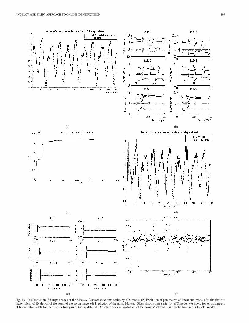
The proposed approach has been tested on a benchmarkproblem: the Mackey–Glass chaotic time series prediction andthe results compared to those generated by alternative tech-niques for online learning TS models, published in references[31] and [34]. The chaotic time series is generated from theMackey–Glass differential delay equation defined by [16], [31]

The aim is using the past values of to predict some futurevalue of . We assume , and the value of thesignal 85 steps ahead is predicted (same as in [31])based on the values of the signal at the current moment, 6, 12,and 18 steps back

The validation data set consists of 500 data samples. The samenondimensional error index (NDEI) defined as the ratio of theroot mean square error over the standard deviation of the targetdata is used as in [31]–[34] to compare model performance.

The results summarized in Table III and Fig. 13 show thatthe new approach can yield a compact model with favorablycomparable NDEI. It should be noted that TS models with lowerNDEI have been reported in [31]–[34]. The number of rules(nodes or units) of these models is, however, in the range ofa thousand which significantly undermines their transparencyan interpretability. ETS model has evolved in online mode to113 transparent rules with . It should also benoted that similar approach to the one presented in this paper,


(a)

(b)

Fig. 11 Evolution of parameters of consequent part (global criteria).

but using nonrecursive moving window [35] yields for the sameproblem evolving to 35 rules.

In order to test the robustness of the eTS model a 5% randomnoise has been added to the standard Mackey–Glass time series.The eTS model has evolved to 124 rules with different centersand the . From Fig. 13(d) and Fig. 13(f) itcan be seen that initially the error is higher, but the TS modelquickly up-grades its structure and reduces the error. Fig. 13(e)illustrates the evolution of the parameters of the first six fuzzyrules, which is similar to the case when no noise is consideredin the data.

VI. CONCLUSION

An approach to online identification of ETS models is pro-posed in the paper. It is computationally effective, as it doesnot require re-training of the whole model. It is based on re-cursive, noniterative building of the rule base by unsupervised

(a)

(b)

Fig. 12 (a) Evolution of the norm of the co-variance (global estimation). (b)Evolution of the norm of the co-variance (local estimation).

TABLE IIICOMPARISON OF ETS WITH OTHER EVOLVING MODELS

learning. The rule-based model evolves by replacement or up-grade of rules and parameter estimation.

The adaptive nature of this model in addition to the highlytransparent and compact form of fuzzy rules makes thema promising candidate for online modeling and control ofcomplex processes competitive to neural networks. The mainadvantages of the approach are:


(a) (b)

(c) (d)

(e) (f)

Fig. 13 (a) Prediction (85 steps ahead) of the Mackey-Glass chaotic time series by eTS model. (b) Evolution of parameters of linear sub-models for the first sixfuzzy rules. (c) Evolution of the norm of the co-variance. (d) Prediction of the noisy Mackey-Glass chaotic time series by eTS model. (e) Evolution of parametersof linear sub-models for the first six fuzzy rules (noisy data). (f) Absolute error in prediction of the noisy Mackey-Glass chaotic time series by eTS model.


1) it can develop/evolve an existing model when the datapattern changes, while inheriting the rule base;

2) it can start to learn a process from a single data sample andimprove the performance of the model predictions online;

3) it is noniterative and recursive and hence computation-ally very effective (the time necessary for calculation is afraction of a second for a new data sample using a stan-dard PC).

The proposed concept, has wide implications for many fields,including nonlinear adaptive control, fault detection and diag-nostics, performance analysis of dynamical systems, time-se-ries and forecasting, knowledge extraction, intelligent agents,behavior and modeling. The results illustrate the viability, effi-ciency and the potential of the approach when used with a lim-ited amount of initial information, especially important in au-tonomous systems and robotics. Future implementation in var-ious engineering problems is under consideration.

APPENDIX

A. WEIGHTED RECURSIVE LEAST SQUARES ALGORITHM

The wRLS algorithm could be derived from the weightedpseudo-inversion (16) expressing the matrices as sums and re-grouping the components in a similar way as RLS is derivedfrom LS [2], [30]

(A1)

where is the co-variance matrix.Using this expression for the estimate based on data and

regrouping we have

(A2)

Substituting (A2) in (A1) and using the matrix inversion Lemma(Lemma 3.1 from [30], p. 65) we arrive at

(A3)

which is equivalent to (17). In a similar way, from the definitionof the co-variance matrix for the estimation based on data wehave

(A4)

which is equivalent to (18).

B. RECURSIVE POTENTIALS CALCULATION

Starting form the formula of the potential (19) and expressingthe projections of the distances in an explicit form for the timestep we have

(A5)Regrouping we have (A6) shown at the bottom of the page,which is equivalent to (20).

C. RECURSIVE UPDATE OF FOCAL POINT’S POTENTIAL

If a data point is accepted to be the focal point of a cluster/ruleat time ( ; for ) then its potential iscalculated according to (19) as

(A7)

We can re-order expressing the sums explicitly

(A8)

At the next time step the potential have to be updated inorder to accommodate the influence of the new data on thiscenter

(A9)

By substituting (A8) into (A9) we have

(A10)

By regrouping, we arrive at (A11) shown at the top of the nextpage, which is equivalent to (21).

D. CO-VARIANCE MATRIX UPDATE

Let us introduce a vector of inputs that are weighted by thenonnormalized firing levels of the rules similarly to the nota-tions used in (10) as

(A12)

(A6)


(A11)

Then it is obvious that

(A12a)

From the expression for the Kalman filter for the update of theco-variance matrices (12) we have

(A13)

or expressing the history until time in an explicit way

(A14)

where ; ;

Let us suppose that the rule added atthe step had been added from the beginning. Then theco-variance matrix at time would be

or

(A15)

where ; . It can be seen thatadding a rule at time step results in a corruption of the co-vari-ance matrix, which is expressed in an increase of the denomi-nator of the part subtracted from . It should be notedthat the values of and are strongly less than 1 (becausethey are quadratic forms of membership functions). could bea big number since it is a quadratic form of the input data multi-plied by the co-variance matrix. is bigger then since it is asum of positive membership functions, while is only oneMF. F is also bigger than if . There-fore, the role of the addends would be more significant only ifall values of (for all past time steps) tend to 0 or the co-vari-ance matrix tends to zero. The practical tests with a number offunctions illustrate that the corruption of the covariance matrixby the addition of a new rule is marginal.

We approximate this (normally small) influence by an in-verse mean of average type of correction. The logic is following.From (A14), (A15) we have that the corrupted co-variance ma-trix is a function of the original one

(A16)

An approximation of the function could be the inverse squaredmean, since the role of the corruption will decrease with increaseof and this is a squared dependence

(A17)

which is equivalent to (25).

REFERENCES

[1] D. Specht, “A general regression neural network,” IEEE Trans. NeuralNetworks, vol. 2, pp. 568–576, Nov. 1991.

[2] L. Ljung, System Identification, Theory for the User. EnglewoodCliffs, NJ: Prentice-Hall, 1987.

[3] R. R. Yager and D. P. Filev, Essentials of Fuzzy Modeling and Con-trol. New York: Wiley, 1994.

[4] T. A. Johanson and R. Murray-Smith, “Operating regime approach tononlinear modeling and control,” in Multiple Model Approaches to Mod-eling and Control, R. Murray-Smith and T. A. Johanson, Eds. Hants,U.K.: Taylor Francis, pp. 3–72.

[5] J. S. R. Jang, “ANFIS: adaptive network-based fuzzy inference sys-tems,” IEEE Trans. Syst., Man Cybern., vol. 23, pp. 665–685, May/June1993.

[6] C. K. Chiang, H.-Y. Chung, and J. J. Lin, “A self-learning fuzzy logiccontroller using genetic algorithms with reinforcements,” IEEE Trans.Fuzzy Syst., vol. 5, pp. 460–467, Aug. 1997.

[7] P. P. Angelov, V. I. Hanby, R. A. Buswell, and J. A. Wright, “Auto-matic generation of fuzzy rule-based models from data by genetic al-gorithms,” in Advances in Soft Computing, R. John and R. Birkenhead,Eds. Heidelberg, Germany: Springer-Verlag, 2001, pp. 31–40.

[8] F. Hoffmann and G. Pfister, “Learning of a fuzzy control rule base usingmessy genetic algorithms,” in Studies in Fuzziness and Soft Computing,F. Herrera and J.L. Verdegay, Eds. Heidelberg, Germany: PhysicaVerlag, 1996, vol. 8, pp. 279–305.

[9] P. P. Angelov, Evolving Rule-Based Models: A Tool for Design of Flex-ible Adaptive Systems. Heidelberg, Germany: Springer-Verlag, 2002.

[10] B. Carse, T. C. Fogarty, and A. Munro, “Evolving fuzzy rule-based con-trollers using GA,” Fuzzy Sets Syst., vol. 80, pp. 273–294, 1996.

[11] P. P. Angelov, V. I. Hanby, and J. A. Wright, “HVAC systems simulation:a self-structuring fuzzy rule-based approach,” Int. J. Architectural Sci.,vol. 1, no. 1, pp. 49–58, 2000.

[12] K. Shimojima, T. Fukuda, and Y. Hasegawa, “Self-tuning fuzzy mod-eling with adaptive membership function, rules, and hierarchical struc-ture based on genetic algorithm,” Fuzzy Sets Syst., vol. 71, pp. 295–309,1995.

[13] T. Takagi and M. Sugeno, “Fuzzy identification of systems and its appli-cation to modeling and control,” IEEE Trans. Syst., Man Cybern., vol.15, pp. 116–132, 1985.

[14] M. Sugeno and M. Yasukawa, “A fuzzy logic based approach ot quali-tative modeling,” IEEE Trans. Fuzzy Syst., vol. 1, pp. 7–31, Feb. 1993.

[15] D. P. Filev, T. Larsson, and L. Ma, “Intelligent control for automotivemanufacturing-rule based guided adaptation,” in Proc. IEEE Conf.IECON’00, Nagoya, Japan, Oct. 2000, pp. 283–288.

[16] S. L. Chiu, “Fuzzy model identification based on cluster estimation,” J.Intel. Fuzzy Syst., vol. 2, pp. 267–278, 1994.

[17] J. Bezdek, “Cluster validity with fuzzy sets,” J. Cybern., vol. 3, no. 3,pp. 58–71, 1974.

[18] J. Yen, L. Wang, and C. W. Gillespie, “Improving the interpretabilityof TSK fuzzy models by combining global and local learning,” IEEETrans. Fuzzy Syst., vol. 6, pp. 530–537, Nov. 1998.

[19] EUNITE: EUropean network on intelligent technologies for smart adap-tive systems, p. 4, 2000.

[20] F.-J. Lin, C.-H. Lin, and P.-H. Shen, “Self-constructing fuzzy neural net-work speed controller for permanent-magnet synchronous motor drive,”IEEE Trans. Fuzzy Syst., vol. 9, pp. 751–759, Oct. 2001.


[21] H. R. Berenji, “A reinforcement learning-based architecture for fuzzylogic control,” Int. J. Approx. Reasoning, vol. 6, pp. 267–292, 1992.

[22] G. G. Yen and P. Meesad, “An effective neuro-fuzzy paradigm for ma-chinery condition health monitoring,” in Proc. IEEE Int. Joint Conf.IJCNN’99, Washington, DC, 1999, pp. 1567–1572.

[23] D. E. Gustafson and W. C. Kessel, “Fuzzy clustering with a fuzzy co-variance matrix,” in Proc. IEEE Control Decision Conf., San Diego, CA,1979, pp. 761–766.

[24] F. Klawon and P. E. Klement, “Mathematical analysis of fuzzy classi-fiers,” Lect. Notes Comp. Sci., vol. 1280, pp. 359–370, 1997.

[25] R. R. Yager and D. P. Filev, “Learning of fuzzy rules by mountain clus-tering,” in Proc. SPIE Conf. Applicat. Fuzzy Logic Technol., Boston,MA, 1993, pp. 246–254.

[26] K. L. Anderson, G. L. Blackenship, and L. G. Lebow, “A rule-basedadaptive PID controller,” in Proc. 27th IEEE CDC’88, 1988, pp.564–569.

[27] D. P. Filev, “Rule-base guided adaptation for mode detection in processcontrol,” in Proc. Joint 9th IFSA World Congr./20th NAFIPS Annu.Conf., Vancouver, BC, Canada, July 2001, pp. 1068–1073.

[28] R. Babuska, “Fuzzy modeling and identification,” Ph.D. thesis, Univ. ofDelft, Delft, The Netherlands, 1996.

[29] J. Moody and C. J. Darken, “Fast learning in networks of locally-tunedprocessing units,” Neural Computat., vol. 1, pp. 281–294, 1989.

[30] K. J. Astroem and B. Wittenmark, Adaptive Control. Reading, MA:Addison-Wesley, 1989.

[31] N. K. Kasabov and Q. Song, “DENFIS: dynamic evolving neural-fuzzyinference system and its application for time-series prediction,” IEEETrans. Fuzzy Syst., vol. 10, pp. 144–154, Apr. 2002.

[32] J. Platt, “A resource allocation network for function interpolation,”Neural Computat., vol. 3, pp. 213–225, 1991.

[33] D. Deng and N. Kasabov, “Evolving self-organizing maps for onlinelearning, data analysis and modeling,” in Proc. IJCNN’2000 Neural Net-works, Neural Comput.: New Challenges Perspectives New Millennium,vol. VI, S.-I. Amari, C. L. Giles, M. Gori, and V. Piuri, Eds., New York,NY, 2000, pp. 3–8.

[34] N. Kasabov, “Evolving fuzzy neural networks—algorithms, applicationsand biological motivation,” in Methodologies for the Conception, De-sign and Application of Soft Computing, T. Yamakawa and G. Mat-sumoto, Eds, Singapore: World Scientific, 1998, pp. 271–274.

[35] P. Angelov and R. Buswell, “Identification of evolving fuzzy rule-basedmodels,” IEEE Trans. Fuzzy Syst., vol. 10, pp. 667–677, Oct. 2002.

Plamen P. Angelov (M’99) received the Ph.D. degree from the BulgarianAcademy of Science, Bulgaria, in 1993.

Since June 2003, he has been a Lecturer in the Department of Communica-tions Systems, Lancaster University, Lancaster, U.K. He was a Research Fellowin Loughborough University, U.K., from 1998 to 2003. He has been VisitingResearch Fellow in CESAME, Catholic University of Louvain, Belgium, in1997, Hannover University and HKI, Jena, Germany, from 1995 to 1996. He au-thored the monograph Evolving Rule based Models: A Tool for Design of Flex-ible Adaptive Systems (Heidelberg, Germany: Springer, 2002). His research hasbeen funded by the EC, ASHARE, Research Councils of UK (EPSRC), Ger-many (DAAD and DFG), Belgium, Italy (CNR), Bulgaria (NFSI). His researchinterests are in intelligent data processing, particularly in evolving rule-basedmodels, self-organizing and autonomous systems, evolutionary algorithms, op-timization and optimal control in a fuzzy environment.

Dr. Angelov has been in the program and organizing committees of severalconferences, including IFSA-2003, GECCO-2002, RASC-2002, FUBEST’94and ’96, BioPS’94, ’95, ’97.

Dimitar P. Filev (M’95–SM’97) received the PhD. degree in electrical engi-neering from the Czech Technical University, Czechoslovakia, in 1979.

He is a Staff Technical Specialist and a Manager of the Knowledge Based Sys-tems and Control Department with Advanced Manufacturing Technology De-velopment, Ford Motor Company specializing in industrial intelligent systemsand technologies for control, diagnostics and decision making. Prior to joiningFord, he was Professor of information systems and Senior Research Associateat the Machine Intelligence Institute, Iona College, and Associate Professor atthe Bulgarian Academy of Sciences. He is conducting research in control theoryand applications, modeling of complex systems, and intelligent modeling andcontrol. He has published three books and over 150 articles in refereed journalsand conference proceedings. He holds nine U.S. patents.

Dr. Filev received the 1995 Award for Excellence from MCB University Pressand three Henry Ford Technology Awards. He is an Associate Editor of the IEEETRANSACTIONS. ON FUZZY SYSTEMS, the International Journal of General Sys-tems, and the International Journal of Approximate Reasoning.

an approach to on-line identification of takagi-sugeno...

Documents