an animated guide©: proc ucm (unobserved components model) · 2014-01-06 · an animated guide©:...

An Animated Guide©: Proc UCM (Unobserved Components Model) Russ Lavery, Contractor for ASG, Inc.

ABSTRACT This paper explores the underlying model and several of the features of Proc UCM, new in the Econometrics and Time Series (ETS) module of SAS . This procedure can be used by programmers in many fields, not just Econometrics. Time series data is generated by marketers as they monitor “sales by month” and by medical researchers who collect vital sign information over time. This technique is well suited to modeling the effect of interventions (drug administration or a change in a marketing plan). This new procedure combines the flexibility of Proc ARIMA with the ease of use and interpretability of Smoothing models. UCM does not have the capability to easily model transfer functions, a useful ARIMA function that is planned for Proc UCM.

INTRODUCTION This paper explains the underlying model several of the features of Proc UCM, new in the Econometrics and Time Series (ETS) module. This procedure can be used by programmers in many fields, not just Econometrics. Time series data is generated by marketers as they monitor “sales by month” and by medical researchers who collect vital sign information over time. This technique is well suited to modeling the effect of interventions (drug administration or a change in a marketing plan). This new procedure combines the flexibility of Proc ARIMA with the ease of use and interpretability of Smoothing models.

THE MODEL NEW DEFINITIONS One thing that makes UCM useful is its similarity to regression. A useful conceptual framework for UCM is that of a regression model (Y= B0 + B1X1 +B2X2 + ε ) where the betas are allowed to be time varying. A major difference between data properly modeled with regression and data typically modeled by time series techniques is the presence of auotocorrelation, or serial correlation. In “time series data” observations close together tend to behave similarly. If observation number n is above a fitted regression line, it is likely that observations N-1 and N+1 will also be above the regression line. This pattern of correlation between observations (and errors) breaks down as observations get farther apart in time. These characteristics suggest that a model for the data should place more “weight” or “importance” on “recent” observations and not give all observations in the data set equal importance. Proc ARIMA, and Proc UCM, both create models that are “local”, that is they attribute more importance to “close” observations. The model for UCM is: Yt = µt + γt + ψt + rt + Σ φi Yt-1 Yt = trend + Season + Cycle + Autoregressive term + A regressive terms involving lagged dep. Variables + Σ βj Xjt + εt + A regressive term on indep. vars. + error term The model components µt, , γt , ψt and rt are assumed to be independent of each other and model underlying “drivers” of the time series.

of 23

AnalysisNESUG 17

Yt Dependent Variable

µt Trend is implemented through the combination of level and slope statements, and their options. A UCM with just a level statement, models a time series with 0 slope. A UCM with just a slope statement gives an error.

Trend is the natural tendency of a series in the absence of seasonality, cycles or the effect of any independent variables. In UCM, this is a mean and a slope, so it corresponds to B0 and B1 in regression. Trend is modeled in two ways and it’s relationship to B0 and B1 can be seen below. One method is a random walk µt = µt –1 + ή (where ή is an IID error term). The second method is a locally linear trend with a slope that varies, only, with time. µt = µt –1 + βt –1 + ήt (where ή is ~i.i.d N(0, σ2 ή IID error term). As beta goes forward, it can vary with time as βt –1 = βt –1 + ζt (where ζ is is ~i.i.d N(0, σ2

ζ IID error term).

γt Season is implemented through the season statement and it’s options.

Season is the effect of seasonal effects and does not imply a yearly period to the season. The main characteristic of seasonally is that it’s period (the time it takes to get through one full cycle) is known. The effects of seasonality sum to zero over the cycle. Seasonality is modeled in two ways. One method is a dummy variable method

Σγ = ωt (where ωt is ~i.i.d N(0, σ2ω IID error term).

The second method is a Uses a trigonometric form and seasonality is the sum of different cycles. Proc UCM allows blocking of cycles, or specifying cycles within cycles. The need for this can occurr in many instances. One example is admissions at an Emergency Room. There is a weekly cycle, where Monday admissions are low and Saturday admissions are high. There is also a daily cycle that starts slow in early AM and has early PM and evening peaks. These cycles of admission nest and produce very high admissions on Saturday evening.

ψt Cycle is important Cycles are like seasons, but with an unknown period. They are not often

used in their “pure form”, but are employed as building blocks. Cycle effects are similar to seasonal effects but the period is not known and determined from the data. A periodic pattern, no matter how complex, can be expressed as a sum of cycles. UCM has implemented cycles as having fixed periods but time varying amplitude and phase.

rt Autoregressive term UCM considers an autoregressive term as a cycle where frequency is either

0 or π. The expression for UCM autoregression is: rt = ρ rt-1 + υt (where υ is ~i.i.d N(0, σ2 υ IID error term).

Σ φi Yt-1 A regressive terms involving lagged dep. Variables

Σ βj Xjt A regressive term on indep. vars.

These two terms allow the programmer/statistician to great flexibility in describing the process under study. Σ βj Xjt allows the determination of effects of outside intervention and support dummy variable and continuous variable coding. They can be used to model the effect of investigator interventions like drug administration or a change in a marketing plan.

εt Irregular term or error term εt is ~i.i.d N(0, σ2

ε IID error term).

The programmer/statistician can create a great many types of time series by adding and deleting components from the model as well as changing options associated with statements in the model. Some knowledge of this is required because the determination of the best model will involve a process that is similar to the stepwise removal process in regression. While a parsimonious model is the goal of any modeling project, there is no general agreement in the literature on how this is best to be done. This paper, not in conflict with the literature but perhaps foolishly, makes an attempt to simplify a model. UCM output parameters are different from regression and this has impact on how UCM is used. Proc UCM can

of 23

AnalysisNESUG 17

interpolate missing/new values of Y within the time span of the estimating data set. It can also forecast future values of Y. UCM produces two tables that show components of the model and their associated P values. Below, please find some rules on interpreting these P values and how the interpretation can be used to purify the model.

1) variances of the disturbance terms of the unobserved components -if not significant, the term is not time varying and should be made deterministic

2) Dampening coefficients and Frequency of cycles-

-if not significant, the term is not contributing to the model and should be removed

3) Dampening coefficient of autoregression terms

- If not significant, the term is not contributing to the model and should be removed

4) Regression coefficient of Regression terms

-if not significant, the term is not contributing to the model and should be removed

UCM allows the programmer/statistician to set the above parameters to a specific value. This is important because the stepwise process of improving the model involves: 1) removing statements from the model to remove an underlying process from the model and/or 2) setting variance parameters to zero to change the associated underlying process from time varying to fixed. As an example of changing the form of the model by setting parameters to be fixed at zero, examine the sub-models below that are associated with trend. Trend, we should remember, is only one component of the model. The common conditions of the UCM, that of a locally linear trend is implied in the two equations below. µt = µt -1 + βt –1 + ήt (where ή is ~i.i.d N(0, σ2 ή IID error term) Interpret this as the mean of the current period =last period’s mean, + effect of 1 period of time + a random term βt –1 = βt –1 + ζt (where ζ is ~i.i.d N(0, σ2

ζ IID error term). Interpret this as the slope changes randomly. The change is the effect of “time” and not an independent variable.

If σ2ζ = 0 Bt=Bt-1 or B is a constant. This transforms the above equations to just one.

µt = µt -1 + β + ήt .

This is called a linear trend with fixed slope model

If σ2ή = 0 This transforms the above equations to:

µt = µt -1 + βt –1 + 0 <-- like the model above but with one less error term. βt –1 = βt –1 + ζt (where ζ is ~i.i.d N(0, σ2

ζ IID error term). Which often produces a smoother trend than the original two equation UCM model.

If both σ2ζ = 0 and σ2

ή = 0 B is a constant and there is no error term in the trend component. The trend is no longer random and is modeled as: µt = µo + βt

PROJECT1 To demonstrate Proc UCM, a dataset was created by data step programming. Components of the UCM model

of 23

AnalysisNESUG 17

were calculated individually in a datastep and summed to get the total sales, shown below. The program is attached to the article. The task was to use Proc UCM to model this dataset. .

To the right is a plot of total sales for the hypothetical company. The company makes a very high tech kind of eyeglasses. These glasses are appropriate for High altitude hiking, where UV is strong and where there is likelihood of reflection off the ground. The imaginary glasses are sold to high altitude hikers and to construction workers, and others, who work in areas of high ground/water reflectivity. There was a yearlong recession from month 12 to 24 (see vertical lines) and there was a different effect on the retail vs commercial sales. Both were affected, but retail sales were affected more due to a large reduction in travel vacations (to high altitude spots). Commercial was affected, but not as much. During the recession, the company decided to expand internationally and started shipping to the southern hemisphere (the company calls this volume “Sales to Antarctica” though shipments go to New Zealand a, Peru and other destinations). Since the winter/summer seasons are reversed, the seasonality of total sales was changed. International sales started the same month that the recession ended.

OUT HYPOTHETICAL MANAGEMENT ISSUE IS TO DETERMINE THE EFFECT OF THE RECESSION AND OF THE STRATEGIC DECISION TO “GO INTERNATIONAL”.

The figure to the right shows how the three cycles (retail construction/commercial and Antarctic) are out of phase and how they add to the total cycle component for the data set. As American sales started to tail off the international sales (New Zealand, Australia, Peru) started up and not only drove the total sales up, but extended the selling “season”.

of 23

AnalysisNESUG 17

This chart shows the trends of the components of the model. The blue line shows the calculated trend in the international sales. There were no international sales until the recession forced the company to a strategic change. The red line shows that the recession made retail sales flat during the recession. The green line, the commercial trend, shows that the people who used the glasses at work, continued to buy through the recession, though at a lower rate. To the right is a plot of the summed cycle components that were calculated by data step programming. The business challenge was to remove this noise and to recover the effect of the recession and of going international.

The code submitted, matched by some explanation of the commands, is shown below: Proc UCM data=for_ucm PRINTALL ; id idmonth interval=month; model tot_sales =Rcsn_dv Int_DV; irregular ; level ; slope; cycle; SEASON LENGTH=12 TYPE=TRIG ; deplag lags=1; estimate OUTEST=UCM_ESTIMATES; forecast lead=6 print=decomp OUTFOR=UCM_FORECASTS ; run;

Printall turns on all printing options for the procedure. ID specifies a variable to be used as an identifier. The model statement says Y is total sales and is to be explained by a time series and two independent variables. Irregular instructs SAS to include the error term (irregular term) εt in the model. Level and slope, with no options, combine to tell Proc UCM to model with time varying slope and mean. Cycle says include a cyclical component. This behavior is complex. The season statement and options instruct SAS to look for a 12-month cycle and not to use the dummy variable coding. The observed cyclical behavior seems to be too irregular for dummy variable coding. Deplags 1 instructs SAS to include φi Yt-1 in the model. φI will be estimated from the model. The estimate command tells SAS to estimate parameters and put them in a file called UCM_ESTIMATES. The forecast command tells SAS to forecast values for 6 periods, to calculate the components of the model and put them in a file called UCM_FORECASTS

of 23

AnalysisNESUG 17

The procedure outputs several sub-tables that will be described and not included in this paper First, UCM prints some summary statistics on the data that was used for creation of the model. This includes min, max, mean, date of first obs. and date of last obs. This information is useful in data checking and is a valuable QC feature. Second, UCM prints some summary statistics on the data that was used for estimation. This includes min, max, mean, date of first obs. and date of last obs. One method for forecasting future observations is to put them in the input data set with no Y values. Additionally, programmers/statistician can check to see how well the model is performing by using options to tell SAS to not use the last n observations in the data set (which do have Y values) in creating the model. This allows the model to forecast these time periods and the programmer/statistician to check forecasted vs actual values. This information is useful in model checking. Included tables are: The two tables that must be examined as part of the model selection (stepwise process) are shown below. They are the “Final Estimates of the Free Parameters“ table and the “Significance Analysis of Components (Based on the Final State) “ tables. The parameters of the models, as reported above, are a mixture of variance components and regression-like parameter estimates (Rcsn_dv, Int_DV and DepLag). Variance parameters show up in both tables. Regression-like parameters only show up in one. These different types of parameters have different uses. While the literature has not shown agreement on a procedure for creating a parsimonious model, stepwise logic has not been judged incorrect and can produce a model that predicts and is interesting. For Regression-like parameters: If there are insignificant p-values, the variables should be eliminated, one variable at a time, in a stepwise fashion. The worst performing variable should be eliminated first. For variance type parameters: Creating a parsimonious model involves two steps. The first step is to decide if the component of the model is time varying. The second step is to determine if is contributing. The starting assumption is that the components (Irregular, slope, cycle and season) are both time varying and significant. This model shows indications that these assumptions are not true (see bold below). A component can be significant but not time varying. This means that the non-stochastic part of the component could be left in the model, but as deterministic contributor to Y (like parameters in a regression). A component of the model can not be time varying and “not significant”. A rough outline of the process for making the time varying parts of the model parsimonious is: The output from our first model is:

Is the variance estimate a significant effect?

No

Yes Keep in the model as deterministic! Set Variance =0 and NoEst options

Remove from Model. TWO strikes and you’re OUT!

Is the component significant?

This is not a random effect, but this parameter might have a deterministic effect.

No

Very complex area and beyond the scope of this paper. Theoretical knowledge, from other research, often plays a large part here.

No

Yes

Is the component estimate a significant effect?

Looks like a random effect might exist for this component.

Yes

of 23

AnalysisNESUG 17

Final Estimates of the Free Parameters

Approx Approx

Component Parameter Estimate Std Error t Value Pr > |t|

Irregular Error Variance 0.00001323 8.60115E-6 1.54 0.1241

Level Error Variance 6.50277E-12 7.94696E-9 0.00 0.9993

Slope Error Variance 0.00000483 1.41347E-6 3.42 0.0006

Season Error Variance 0.00001169 2.76826E-6 4.22 <.0001

Cycle Damping Factor 0.93881 0.04069 23.07 <.0001

Cycle Period 16.60643 2.22289 7.47 <.0001

Cycle Error Variance 7.006927E-7 6.11491E-7 1.15 0.2518 Rcsn_dv Coefficient 3.55172 0.04018 88.40 <.0001

Int_DV Coefficient 5.67481 0.06373 89.04 <.0001

DEPLAG PHI_1 0.34053 0.02848 11.96 <.0001

Significance Analysis of Components (Based on the Final State)

Component DF Chi-Square Pr > ChiSq

Irregular 1 0.00 0.9868

Level 1 37311.7 <.0001

Slope 1 4073.99 <.0001

Cycle 2 0.94 0.6241

Season 11 113948 <.0001

Full Model

Step two would be to remove level (modify the model for the highest P value in the Free parameter table) as a time varying component of the model by adding the options Variance=0 and NoEst to the level statement. This option tells Proc UCM to start the model with a variance estimate equal to zero, and not to attempt to estimate a better value (fix the value at zero). The code for step two is below.

Proc UCM data=for_ucm PRINTALL ; id idmonth interval=month; model tot_sales=Rcsn_dv Int_DV;

irregular ; level variance=0 Noest ; slope; cycle;

SEASON LENGTH=12 TYPE=TRIG ; Deplag lags=1; estimate OUTEST=UCM_ESTIMATES; forecast lead=6 print=decomp OUTFOR=UCM_FORECASTS ;run;

Printall turns on all printing options for the procedure. ID specifies a variable to be used as an identifier. The model statement says Y is total sales and is to be explained by a time series and two independent variables Irregular instructs SAS to include the error term (irregular term) εt in the model. The variance of this time varying component, level, has been assigned a staring estimate of at 0 with the NOEST option - to make level NOT time variant. NoEst tells SAS not to try to estimate the variance from the data. Slope can still be time varying. Cycle says include a cyclical component. The season statement and options instruct SAS to look for a 12-month cycle and not to use the dummy variable coding. The observed cyclical behavior seems to be too irregular for dummy variable coding. Deplags 1 instructs SAS to include φi Yt-1 in the model. φI will be estimated from the model. The estimate command tells SAS to estimate parameters and put them in a file called UCM_ESTIMATES. The forecast command tells SAS to forecast values for 6 periods, to calculate the components of the model and put them in a file called UCM_FORECASTS.

The SAS output is below:

of 23

AnalysisNESUG 17


Approx Approx


Irregular Error Variance 0.00001323 8.60123E-6 1.54 0.1241




Cycle Period 16.60643 2.22861 7.45 <.0001

Cycle Error Variance 7.006937E-7 6.11598E-7 1.15 0.2519

Rcsn_dv Coefficient 3.55172 0.04018 88.40 <.0001


DEPLAG PHI_1 0.34053 0.02848 11.96 <.0001



Irregular 1 0.00 0.9868

Level 1 37311.7 <.0001

Slope 1 4073.99 <.0001

Cycle 2 0.94 0.6241

Season 11 113948 <.0001 Step three would be to remove irregular (modify the model for the highest P value in the Free parameter table) as a time varying component of the model by adding the options Variance=0 and NoEst =(variance) to the cycle statement. It does not seem to be significant but, alternatively, it might be mis-specified. The logic is that a mis-specified variable can look insignificant. Try to properly specify it (usually only two ways to specify it) before removing it from the model. The code for step three is below.

Proc UCM data=for_ucm PRINTALL ; id idmonth interval=month; model tot_sales=Rcsn_dv Int_DV ; irregular variance=0 noest; level variance=0 noest; slope; cycle; SEASON LENGTH=12 TYPE=TRIG ; deplag lags=1; estimate OUTEST=UCM_ESTIMATES; forecast lead=6 print=decomp OUTFOR=UCM_FORECASTS ; run;

Printall turns on all printing options for the procedure ID specifies a variable to be used as an identifier Y is total sales and is to be explained by a time series and two independent variables Irregular instructs SAS to include the error term (irregular term) εt in the model The variance of this time varying component has been assigned a staring estimate of at 0 to make it NOT time variant. NoEst tells SAS not to try to estimate the variance from the data. Slope can still be time varying. Cycle has been commented out of the model. The season statement and options instruct SAS to look for a 12-month cycle and not to use the dummy variable coding. The observed cyclical behavior seems to be too irregular for dummy variable coding. Deplags 1 instructs SAS to include φi Yt-1 in the model. φI will be estimated from the model. The estimate command tells SAS to estimate parameters and put them in a file called UCM_ESTIMATES. The forecast command tells SAS to forecast values for 6 periods, to calculate the components of the model and put them in a file called UCM_FORECASTS.

Model With Level variance=0

of 23

AnalysisNESUG 17


Approx Approx





Cycle Period 6.61696 0.05084 130.15 <.0001

Cycle Error Variance 0.00000222 1.50905E-6 1.47 0.1411



DepLag Phi_1 0.36535 0.02035 17.96 <.0001



Irregular 1 . .

Level 1 40450.6 <.0001

Slope 1 4842.97 <.0001

Cycle 2 0.08 0.9599

Season 11 127708 <.0001

Model With: Level Variance=0 Irregular Variance=0

Step four would be to remove cycle (modify the model for the highest P value in the Free parameter table) as a time varying component of the model by adding the options Variance=0 and NoEst =(variance) to the cycle statement. It does not seem to be significant but, alternatively, it might be mis-specified. The logic is that a mis-specified variable can look insignificant. Try to properly specify it (usually only two ways to specify it) before removing it from the model. The code for step three is below.

Proc UCM data=for_ucm PRINTALL ; id idmonth interval=month; model tot_sales=Rcsn_dv Int_DV ; irregular variance=0 noest; level variance=0 noest; slope; *cycle; SEASON LENGTH=12 TYPE=TRIG ; deplag lags=1; estimate OUTEST=UCM_ESTIMATES; forecast lead=6 print=decomp OUTFOR=UCM_FORECASTS ; run;

Printall turns on all printing options for the procedure ID specifies a variable to be used as an identifier Y is total sales and is to be explained by a time series and two independent variables Irregular instructs SAS to include the error term (irregular term) εt in the model The variance of this time varying component has been assigned a staring estimate of at 0 to make it NOT time variant. NoEst tells SAS not to try to estimate the variance from the data. Slope can still be time varying. Cycle has been commented out of the model. The season statement and options instruct SAS to look for a 12-month cycle and not to use the dummy variable coding. The observed cyclical behavior seems to be too irregular for dummy variable coding. Deplags 1 instructs SAS to include φi Yt-1 in the model. φI will be estimated from the model. The estimate command tells SAS to estimate parameters and put them in a file called UCM_ESTIMATES. The forecast command tells SAS to forecast values for 6 periods, to calculate the components of the model and put them in a file called UCM_FORECASTS.

The SAS output is below:

of 23

AnalysisNESUG 17



Approx Approx





Int_DV Coefficient 5.81361 0.07322 79.40 <.0001 DEPLAG PHI_1 0.34204 0.02439 14.02 <.0001

Significance Analysis of Components

(Based on the Final State)


Irregular 1 . .

Level 1 27514.0 <.0001

Slope 1 2944.99 <.0001

Season 11 89956.5 <.0001

All of these variables are significant, in both tables, though there might well be better models. Cycle was originally put in the model in hopes that it would automatically model the effects of the three different cycles. It did not end up as a strong predictor.

of 23

AnalysisNESUG 17

PROJECT 2 TAKEN FROM SAS DOCUMENTATION The goal of this project is to model some cancer data from the Connecticut Tumor registry as reported by Houghton, Flannery and Viola in the International Journal of Cancer. They calculated the age-adjusted incidence of Melanoma per 100,000 subjects. This data, and sunspot data, is shown in the graph below. The original article did not make any link to sunspot activity (that idea is from a helpful SAS, Inc. employee).

0

1

2

3

4

5

6

1936

1938

1940

1942

1944

1946

1948

1950

1952

1954

1956

1958

1960

1962

1964

1966

1968

Incidence /100k Sun Spots/100

The code for step 1 is

The plot suggests a cycle or seasonality. We will let the data tell us about the cycle. proc ucm data = both; id year interval = year ; model Incidences ; irregular ; level variance=0 noest ; slope variance=0 noest ; cycle plot=smooth ; estimate plot=(residual normal acf); forecast lead=10 plot=(decomp forecasts); run ;

Output is shown below Final Estimates of the Free Parameters

Approx Approx


Irregular Error Variance 0.05706 0.01750 3.26 0.0011


Cycle Period 9.68327 0.62860 15.40 <.0001

Cycle Error Variance 0.00302 0.0022975 1.31 0.1893




Irregular 1 0.03 0.8698

Level 1 3097.46 <.0001

Slope 1 694.83 <.0001

Cycle 2 2.54 0.2810 Damping Final %Relative Cycle

Name Type Period Frequency Factor Amplitude to Level Variance

Cycle Stationary 9.68327 0.64887 0.96476 0.20439 4.29794 0.04356

Cycle is a poor performer, but the plot really seems to show cycles. The old model vs. theory issue arises if we posit a sun connection. While cycle performs poorly, a 9.68327 -year cycle suggests sunspots (to the smart folks at SAS- not to the original authors).

of 23

AnalysisNESUG 17

Step 2 is shown below Sunspot data is available on the web. Get it and create a SAS data set. Use Sunspots and an independent variable in the model.

proc ucm data = both; id year interval = year ; model Incidences = sunspots ; irregular ; level variance=0 noest ; slope variance=0 noest ; cycle plot=smooth ; estimate plot=(residual normal acf); forecast lead=10 plot=(decomp forecasts); run ;

Output is shown below. Final Estimates of the Free Parameters

Approx Approx


Irregular Error Variance 0.11227 0.02807 4.00 <.0001


Cycle Period 2.60497 0.13294 19.59 <.0001

Cycle Error Variance 4.91638E-8 1.94826E-7 0.25 0.8008

sunspots Coefficient 0.00084084 0.0010898 0.77 0.4404 Significance Analysis of Components



Irregular 1 0.15 0.6942

Level 1 1170.86 <.0001

Slope 1 456.73 <.0001

Cycle 2 0.69 0.7075 Dampening Final %Relative Cycle

Name Type Period Frequency Factor Amplitude to Level Variance

Cycle Stationary 2.60497 2.41200 0.99999 0.03292 0.69612 0.00211

With sunspots in the model, cycle is a very poor performer, but the variable sunspots performs poorly as well. Looking at the picture at the start, we can see multicoliniarity. Note that the cycle period (2,60497) does not seem to “agree” with the observed cycle period in the plot.

of 23

AnalysisNESUG 17

The code for step 3 is shown below Follow theory. Keep sunspots in the model and lag them Lag them by two years (or one…or three). Create the lagged variable in a data step (not shown). Folks at SAS found lag two to work well and I will follow their advice. Comment cycle out of the model.

ods html ; ods graphics on ; proc ucm data = both; id year interval = year ; model Incidences =lag2SP; irregular ; level variance=0 noest ; slope variance=0 noest ; *****cycle plot=smooth ; estimate plot=(residual normal acf); forecast lead=10 plot=(decomp forecasts); run ; ods graphics off ; ods html close ;

Output is shown below Final Estimates of the Free Parameters

Approx Approx


Irregular Error Variance 0.06283 0.01524 4.12 <.0001

lag2SP Coefficient 0.00429 0.0007966 5.39 <.0001




Irregular 1 0.73 0.3937

Level 1 1731.59 <.0001

Slope 1 764.32 <.0001

Components of model are strong. All P values are very small. There is a strong sunspot link. With the code above, SAS also gives lots of very interesting and useful output. The output from the final model is shown below.

of 23

AnalysisNESUG 17

Input Data Set Name WORK.BOTH

Time ID Variable year

Estimation Span Summary

Variable Type First Obs Last Obs NObs NMiss Min Max Mean Standard

Deviation Incidences Dependent 1936 1972 37 0 0.80000 4.80000 2.80811 1.23904

lag2SP Predictor 1936 1972 37 0 4.40000 190.20000 75.35135 52.88085

Forecast Span Summary

Variable Type First Obs Last Obs NObs NMis

s Min Max Mean Standard Deviation

Incidences Dependent 1936 1972 37 0 0.80000 4.80000 2.80811 1.23904

lag2SP Predictor 1936 1972 37 0 4.40000 190.20000 75.35135 52.88085

Fixed Parameters in the Model

Component Parameter Value Level Error Variance 0 Slope Error Variance 0

Preliminary Estimates of the Free Parameters

Component Parameter Estimate Irregular Error Variance 3.41052

Likelihood Based Fit Statistics

Full Log-Likelihood -15.04479 Diffuse Part of Log-Likelihood -2.14211

Normalized Residual Sum of Squares 34.00000 Akaike Information Criterion 38.08957

Bayesian Information Criterion 44.53324 Number of non-missing observations used for computing the log-likelihood = 37

Likelihood Optimization Algorithm Converged in 7 Iterations.


Component Parameter Estimate Approx Std Error t Value Approx

Pr > |t| Irregular Error Variance 0.06283 0.01524 4.12 <.0001

lag2SP Coefficient 0.00429 0.0007966 5.39 <.0001

Fit Statistics Based on Residuals

of 23

AnalysisNESUG 17

Mean Squared Error 0.11260 Root Mean Squared Error 0.33556

Mean Absolute Percentage Error 13.00476 Maximum Percent Error 48.79725

R-Square 0.90998 Adjusted R-Square 0.90998

Random Walk R-Square 0.38472 Amemiya's Adjusted R-Square 0.90452

Number of non-missing residuals used for computing the fit statistics = 34


Component DF Chi-Square Pr > ChiSq Irregular 1 0.73 0.3937

Level 1 1731.59 <.0001 Slope 1 764.32 <.0001

of 23

AnalysisNESUG 17

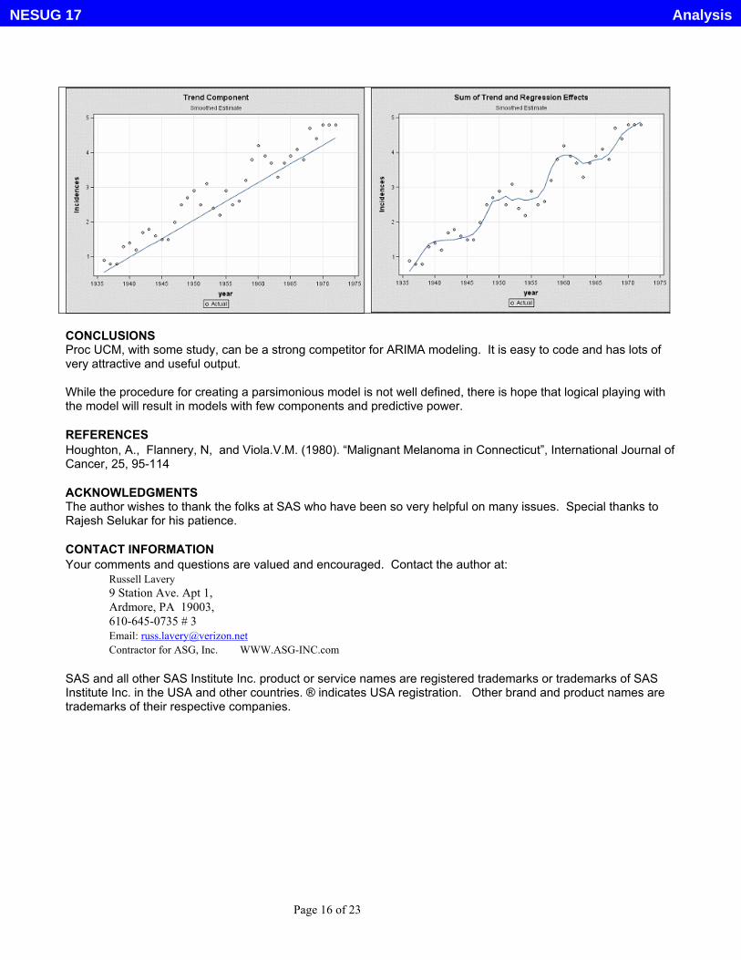
CONCLUSIONS Proc UCM, with some study, can be a strong competitor for ARIMA modeling. It is easy to code and has lots of very attractive and useful output. While the procedure for creating a parsimonious model is not well defined, there is hope that logical playing with the model will result in models with few components and predictive power.

REFERENCES Houghton, A., Flannery, N, and Viola.V.M. (1980). “Malignant Melanoma in Connecticut”, International Journal of Cancer, 25, 95-114

ACKNOWLEDGMENTS The author wishes to thank the folks at SAS who have been so very helpful on many issues. Special thanks to Rajesh Selukar for his patience.

CONTACT INFORMATION Your comments and questions are valued and encouraged. Contact the author at:

Russell Lavery 9 Station Ave. Apt 1,

Ardmore, PA 19003, 610-645-0735 # 3

Email: [email protected] Contractor for ASG, Inc. WWW.ASG-INC.com

SAS and all other SAS Institute Inc. product or service names are registered trademarks or trademarks of SAS Institute Inc. in the USA and other countries. ® indicates USA registration. Other brand and product names are trademarks of their respective companies.

of 23

AnalysisNESUG 17

mailto:[email protected]

**the Sun_glasses project************************************** data for_ucm; retain retail_trend Constr_trend AntA_trend ; infile datalines firstobs=6 missove r; input @1 idmonth monyy7. @9 month 2.0 Rcsn_dv Int_DV ret_rec_fct constr_rec_fct AntA_rec_fct; if _n_=1 then do; /*initialize* / retail_trend=0; Constr_trend=0; AntA_trend =0; end; *Explanation of the recession fctors below: 1=good times 0=no sales at all; *RECESSION FACTORS COULE BE NAMED BETTER. THEY MODIFY THE CYCLE AND THE TRAND; *** TREND SECTION ****; *calculate trend components; *there is a constant trend and a modifier to produce recessions and no sales; *add a bit to last quarters data- we retained it; retail_trend =retail_trend + (.15 *ret_rec_fct );/*if factor is close to 0, little change*/ Constr_trend =constr_trend + (.20 *constr_rec_fct); AntA_trend =AntA_trend + (.10 *AntA_rec_fct ); ** CYCLE SHAPE SECTION ****; *calculate cyclical components - this section sets the shape of the cycle; *domestic retail cycle; if mod(month,12) = (7) then retail_cycle= .9 *ret_rec_fct; /*vacation sales*/ else if mod(month,12) = (8) then retail_cycle= 1.1*ret_rec_fct; else if mod(month,12) = (9 then retail_cycle= .3 *ret_rec_fct; /*poser/school sales*/ )else if mod(month,12) = (11) then retail_cycle=-.2 *ret_rec_fct; /*winter sales downturn*/ else if mod(month,12) = (12) then retail_cycle= .7 *ret_rec_fct; /*holiday sales*/ else if mod(month,12) = (1) then retail_cycle=-.7 *ret_rec_fct; else if mod(month,12) = (2) then retail_cycle=-.9 *ret_rec_fct; else if mod(month,12) = (3) then retail_cycle=-.3 *ret_rec_fct; else retail_cycle =0; *domestic construction cycle ; if mod(month,12) = (7) then constr_cycle=.7 *constr_rec_fct; /*START OF WORK PERIOD*/ else if mod(month,12) = (8) then constr_cycle=.9 *constr_rec_fct; else if mod(month,12) = (9) then constr_cycle=.3 *constr_rec_fct; /*replacing lost items*/ else if mod(month,12) = (11) then constr_cycle=-.3*constr_rec_fct; /*holidays*/ else if mod(month,12) = (1) then constr_cycle=-.7*constr_rec_fct; /* less work in winter*/ else if mod(month,12) = (2) then constr_cycle=-.9*constr_rec_fct; else if mod(month,12) = (3) then constr_cycle=-.3*constr_rec_fct; else constr_cycle =0; *Antarctic sales - Sun from Sept to March - people buy early protection is important; if mod(month,12) = (9) then AntA_cycle= 2 *AntA_rec_fct; /*START OF WORK PERIOD*/ else if mod(month,12) = (10) then AntA_cycle= 1 *AntA_rec_fct; else if mod(month,12) = (11) then AntA_cycle= 1 *AntA_rec_fct; else if mod(month,12) = (12) then AntA_cycle=-.1 *AntA_rec_fct; else if mod(month,12) = (1) then AntA_cycle=-.5 *AntA_rec_fct; /*replacing lost items*/ else if mod(month,12) = (2) then AntA_cycle=-.7 *AntA_rec_fct; else if mod(month,12) = (3) then AntA_cycle=-.2 *AntA_rec_fct; else AntA_cycle =0; ** EXPAND OR CONTRACT THE CYCLE SECTION **; *MODIFY cyclical components - this section sets the magnitude of the cycle; * this section is just to make for easy changes in the curves; retail_cycle =retail_cycle *3 ; *set to three to make it show on plot; constr_cycle =constr_cycle *2 ; AntA_cycle =AntA_cycle *1 ; *ADD UP COMPONENTS SECTION;

of 23

AnalysisNESUG 17

tot_sales =sum(retail_trend,retail_cycle,constr_trend,constr_cycle,AntA_trend,AntA_cycle) ; sumtrend =sum(retail_trend,constr_trend,AntA_trend) ; sumCyc =sum(retail_cycle,constr_cycle,AntA_cycle) ; ** blank Y values for last 6 months so that they can be c=forcasted by this proc; if month GE 73 then do; tot_sales=.; sumtrend =.; sumCyc=.; end; datalines; this is monthly data -- Explanation of the recession fctors below: 1=good times 0=no sales at all -- Cmnth mnth Rcsn_dv Int_DV ret_rec_fct constr_rec_fct AntA_rec_fct Jan2000 01 0 0 .5 1 0 /*good times :-)*/ Feb2000 02 0 0 .5 1 0 /*selling to Us sports and construction*/ Mar2000 03 0 0 .5 1 0 Apr2000 04 0 0 .5 1 0 May2000 05 0 0 .5 1 0 Jun2000 06 0 0 .5 1 0 Jul2000 07 0 0 .5 1 0 Aug2000 08 0 0 .5 1 0 Sep2000 09 0 0 .5 1 0 Oct2000 10 0 0 .5 1 0 Nov2000 11 0 0 .5 1 0 Dec2000 12 1 0 .02 .3 0 /*start of 12 month recession :-( */ Jan2001 13 1 0 .02 .3 0 /* 1 IN Rcsn_dv INDICATES A RECESSION */ Feb2001 14 1 0 .02 .3 0 Mar2001 15 1 0 .02 .3 0 Apr2001 16 1 0 .02 .3 0 May2001 17 1 0 .02 .3 0 Jun2001 18 1 0 .02 .3 0 Jul2001 19 1 0 .02 .3 0 Aug2001 20 1 0 .02 .3 0 Sep2001 21 1 0 .02 .3 0 Oct2001 22 1 0 .02 .3 0 Nov2001 23 1 0 .02 .3 0 /*end of 12 month recession :-) */ Dec2001 24 0 1 .5 1 2 /*Enter international sports market*/ Jan2002 25 0 1 .5 1 2 /*1 IN Int_DV SHOWS INTERNAIONAL SALES*/ Feb2002 26 0 1 .5 1 2 Mar2002 27 0 1 .5 1 2 Apr2002 28 0 1 .5 1 2 May2002 29 0 1 .5 1 2 Jun2002 30 0 1 .5 1 2 Jul2002 31 0 1 .5 1 2 Aug2002 32 0 1 .5 1 2 Sep2002 33 0 1 .5 1 2 Oct2002 34 0 1 .5 1 2 Nov2002 35 0 1 .5 1 2 Dec2002 36 0 1 .5 1 2 Jan2003 37 0 1 .5 1 2 Feb2003 38 0 1 .5 1 2 Mar2003 39 0 1 .5 1 2 Apr2003 40 0 1 .5 1 2 May2003 41 0 1 .5 1 2 Jun2003 42 0 1 .5 1 2 Jul2003 43 0 1 .5 1 2 Aug2003 44 0 1 .5 1 2 Sep2003 45 0 1 .5 1 2 Oct2003 46 0 1 .5 1 2 Nov2003 47 0 1 .5 1 2 Dec2003 48 0 1 .5 1 2 Jan2004 49 0 1 .5 1 2 Feb2004 50 0 1 .5 1 2 Mar2004 51 0 1 .5 1 2 Apr2004 52 0 1 .5 1 2 May2004 53 0 1 .5 1 2 Jun2004 54 0 1 .5 1 2 Jul2004 55 0 1 .5 1 2 Aug2004 56 0 1 .5 1 2

of 23

AnalysisNESUG 17

Sep2004 57 0 1 .5 1 2 Oct2004 58 0 1 .5 1 2 Nov2004 59 0 1 .5 1 2 Dec2004 60 0 1 .5 1 2 Jan2005 61 0 1 .5 1 2 Feb2005 62 0 1 .5 1 2 Mar2005 63 0 1 .5 1 2 Apr2005 64 0 1 .5 1 2 May2005 65 0 1 .5 1 2 Jun2005 66 0 1 .5 1 2 Jul2005 67 0 1 .5 1 2 Aug2005 68 0 1 .5 1 2 Sep2005 69 0 1 .5 1 2 Oct2005 70 0 1 .5 1 2 Nov2005 71 0 1 .5 1 2 Dec2005 72 0 1 .5 1 2 Jan2006 73 0 1 .5 1 2 /*blank calculations and forcast w/ UCM*/ Feb2006 74 0 1 .5 1 2 /*blank calculations and forcast w/ UCM*/ Mar2006 75 0 1 .5 1 2 /*blank calculations and forcast w/ UCM*/ Apr2006 76 0 1 .5 1 2 /*blank calculations and forcast w/ UCM*/ May2006 77 0 1 .5 1 2 /*blank calculations and forcast w/ UCM*/ Jun2006 78 0 1 .5 1 2 /*blank calculations and forcast w/ UCM*/ ; run; **set some display options; symbol1 color=red interpol=join value=dot height=1; run; symbol2 color=green interpol=join value=square height=1; run; symbol3 color=blue interpol=join value=triangle run;

height=1; symbol4 color=black interpol=join value=star height=2; run; legend1 label=none shape=symbol(4,2) position=(top center inside) quit;

mode=share;

**plotting interesting stuff; proc gplot data=for_ucm; title "Show Total Sales and the Sum of the Trends"; plot tot_sales *month sumtrend *month /overlay legend=legend1 href=12 24; run; quit; proc gplot data=for_ucm; *trends; title "Show Cuml sales dut to the trend components"; plot retail_trend *month Constr_trend*month AntA_trend *month /overlay legend=legend1 href=12 24 ;

of 23

AnalysisNESUG 17

run ;quit; proc gplot data=for_ucm; title "Show the monthly Cycle components and the sum of the cycles"; plot sumCyc *month retail_cycle *month constr_cycle *month AntA_cycle *month /overlay legend=legend1 href=12 24; run; quit; proc gplot data=for_ucm; title "Show the Cycle Component"; plot sumCyc*month / legend=legend1 href=12 24; run; quit; titrun;

le "";

***f om Proc UCM data=for_ucm PRINTALL ;

r paper step 1 initial model*****;

id idmonth interval=month; model tot_sales = Rcsn_dv Int_DV ; irregular ; level ; slope; cycle; SEASON LENGTH=12 TYPE=TRIG ; deplag lags=1; estimate OUTEST=UCM_ESTIMATES; forecast lead=6 print=decomp OUTFOR=UCM_FORECASTS ; run; ***from paper step 2 variance of level is set to 0*****; Proc UCM data=for_ucm PRINTALL ; id idmonth interval=month; model tot_sales = Rcsn_dv Int_DV ; irregular ; level variance=0 noest; slope; cycle; SEASON LENGTH=12 TYPE=TRIG ; deplag lags=1; estimate OUTEST=UCM_ESTIMATES; forecast lead=6 print=decomp OUTFOR=UCM_FORECASTS ; run; ***f om Proc UCM data=for_ucm PRINTALL ;

r paper step 3 set irregular to zero*****;

id idmonth interval=month; model tot_sales = Rcsn_dv Int_DV ; irregular variance=0 noest; level variance=0 noest;

of 23

AnalysisNESUG 17

slope; cycle; SEASON LENGTH=12 TYPE=TRIG ; deplag lags=1; estimate OUTEST=UCM_ESTIMATES; forecast lead=6 print=decomp run;

OUTFOR=UCM_FORECASTS ;

***f om Proc UCM data=for_ucm PRINTALL ;

r paper step 4 get rid of cycle*****;

id idmonth interval=month; model tot_sales = Rcsn_dv Int_DV ; irregular variance=0 noest; level variance=0 noest; slope; *cycle; SEASON LENGTH=12 TYPE=TRIG ; deplag lags=1; estimate OUTEST=UCM_ESTIMATES; forecast lead=6 print=decomp run;

OUTFOR=UCM_FORECASTS ;

*****************************sunspot project ***************************************************; data melanoma ; input Incidences @@ ; year = intnx('year','1jan1936'd,_n_-1) ; *year=1936+_n_-1; label Incidences = 'Adg. Inc/100k'; datalines ; 0.9 0.8 0.8 1.3 1.4 1.2 1.7 1.8 1.6 1.5 1.5 2.0 2.5 2.7 2.9 2.5 3.1 2.4 2.2 2.9 2.5 2.6 3.2 3.8 4.2 3.9 3.7 3.3 3.7 3.9 4.1 3.8 4.7 4.4 4.8 4.8 4.8 run ;

;

Proc sort data=melanoma; by run;

year;

data sunspots; infile datalines missover; input @1year @10 sunspots ; year = intnx('year','1jan1931'd,_n_-1) ; format year year4. ; /* http://www1.physik.tu-muenchen.de/~gammel/matpack/html/Astronomy/Sunspots.html#yearly_data 1.2.2 Yearly Data In the table below the yearly sunspot counts from 1700 to 1992 can be found.

of 23

AnalysisNESUG 17

Each M marks a sunspot cycle maximum and each m a minimum. Through 1944 yearly means were calculated as the average of the 12 monthly means. Since 1945 yearly means have been calculated as the average of the daily means. Year Number Year Number Year Number Year Number Year Number */ datalines; 1931 21.2 1932 11.1 1933 5.7 1934 8.7 1935 36.1 1936 79.7 1937 114.4 1938 109.6 1939 88.8 1940 67.8 1941 47.5 1942 30.6 1943 16.3 1944 9.6 1945 33.2 1946 92.6 1947 151.6 1948 136.3 1949 134.7 1950 83.9 1951 69.4 1952 31.5 1953 13.9 1954 4.4 1955 38.0 1956 141.7 1957 190.2 1958 184.8 1959 159.0 1960 112.3 1961 53.9 1962 37.6 1963 27.9 1964 10.2 1965 15.1 1966 47.0 1967 93.8 1968 105.9 1969 105.5 1970 104.5 1971 66.6 1972 68.9 1973 38.0 1974 34.5 1975 15.5 1976 12.6 1977 27.5 1978 92.5 1979 155.4 1980 154.6 1981 140.4 1982 115.9 1983 66.6 1984 45.9 1985 17.9 1986 13.4 1987 29.4 1988 100.2 1989 157.6 1990 142.6 1991 145.7 1992 94.3 ; run ;proc sort data=sunspots; by run;

year;

data both;

of 23

AnalysisNESUG 17

merge sunspots melanoma(in=M) ; by year; smallsun=sunspots/100; * for plotting; lag2SP=lag2(sunspots); if M; run; ods html ; g hics on ; ods rap proc ucm data = both; id year interval = year ; model Incidences ; irregular ; level variance=0 noest ; slope variance=0 noest ; cycle plot=smooth ; estimate plot=(residual normal acf); forecast lead=10 plot=(decomp forecasts); run ; proc ucm data = both; id year interval = year ; model Incidences = sunspots ; irregular ; level variance=0 noest ; slope variance=0 noest ; cycle plot=smooth ; estimate plot=(residual normal acf); forecast lead=10 plot=(decomp forecasts); run ; ods html ; ods graphics on ; proc ucm data = both; id year interval = year ; model Incidences =lag2SP; irregular ; level variance=0 noest ; slope variance=0 noest ; *cycle plot=smooth ; estimate plot=(residual normal acf); forecast lead=10 plot=(decomp forecasts); run ; ods graphics off ; ods html close ;

of 23

AnalysisNESUG 17

an animated guide©: proc ucm (unobserved components model) · 2014-01-06 · an animated guide©:...

Documents