Value Added and Productivity Linkages Across

Countries*

François de Soyres

Toulouse School of Economics

October, 2016

Abstract

What is the relationship between international trade and business cycle synchronization?

Using data from OECD countries, I nd that trade in intermediate inputs plays a signicant

role in synchronizing GDP uctuations across countries while trade in nal goods is found

insignicant. Motivated by this new fact, I build a model of international trade in intermediates

that is able to replicate more than 70% of the empirical trade-comovement slope, making a

signicant step toward solving the Trade Comovement Puzzle. The model relies on two key

assumptions: (i) price distortions due to monopolistic competition and (ii) uctuations in the

mass of rms serving each country. The combination of those ingredients creates a link between

domestic productivity and foreign shocks through trade linkages. Finally, I provide evidence for

the importance of those elements in the link between foreign shocks and domestic GDP and test

other predictions of the model.

Keywords: International Trade, International Business Cycle Comovement, Networks, Input-

Output Linkages

JEL Classication Numbers: F12, F17, F4, F62, L22

*I am indebted to my advisor Thomas Chaney for his invaluable guidance. For their comments, I am grateful toManuel Amador, Ariel Burstein, Patrick Fève, Simon Fuchs, Julian di Giovanni, Christian Hellwig, Oleg Itskhoki,Tim Kehoe, Ellen McGrattan, Marti Mestieri, Alban Moura, Fabrizio Perri, Franck Portier, Ana-Maria Santacreu,Constance de Soyres, Shekhar Tomar, Robert Ulbricht, Kei-Mu Yi and seminar or workshop participants in Uni-versitat Autònoma de Barcelona, the Minneapolis Fed, the Saint-Louis Fed, the University of Minnesota, MidwestMacro Meetings in Rochester, the George Washington Trade Workshop, TSE, UCLA and the SED annual meetingsin Toulouse. Finally, I also thank the Federal Reserve Bank of Minneapolis, where part of this research has beenconducted, for their hospitality and ERC grant N°337272FiNet for nancial support. All errors are mine.

Contact: Toulouse School of Economics, 21 Allée de Brienne, 31000 Toulouse, France. Email:francois.de.soyres@gmail.com.

1

1 Introduction

The Trade Comovement Puzzle, uncovered by Kose and Yi (2001 and 2006), refers to the inability

of international business cycle models to quantitatively account for the high and robust empiri-

cal relationship between international trade and GDP comovement.1 Using dierent versions of

the workhorse international real business cycle (IRBC) model, several authors have succeeded to

qualitatively replicate the positive link between trade and GDP comovement but fall short of the

quantitative relationship by an order of magnitude.2

In this paper, I rene previous empirical investigations of the association between bilateral

trade and GDP comovement and I propose a model that quantitatively accounts for this relation-

ship. First, using data from OECD countries, I show that trade in intermediate inputs plays a

signicant role in synchronizing GDP uctuations across countries while trade in nal goods is

found insignicant, uncovering the strong role of global value chains. Motivated by this new fact, I

then propose a general equilibrium dynamic model of trade in inputs with monopolistic pricing and

rms entry/exit. In the benchmark calibration, the model is able to replicate more than 70% of

the trade-comovement slope, hence proposing a solution for the Trade Comovement Puzzle. The

model features a quantitatively important link between foreign shocks and domestic productivity

through trade linkages suggesting that countries with input-output linkages should have correlated

TFP, a prediction that I validate in the data. Finally, I provide evidence for the role of the key

ingredients generating the quantitative results, namely the importance of price distortions and of

the uctuations of the mass of rms serving every market.

Empirics Since the seminal paper by Frankel and Rose (1998), a large empirical literature has

studied cross countries' GDP synchronization, showing that bilateral trade is an important and

robust determinant of GDP correlation in the cross section. I update those ndings using a panel of

20 OECD countries and uncover a new fact, namely that business cycle synchronization is associated

with trade in intermediate inputs while trade in nal good is found insignicant.

First, I rene previous analysis by constructing a panel dataset consisting of four 10-years time

windows ranging from 1969Q1 to 2008Q4. Controlling for country pair xed eects that can be

correlated with bilateral trade, I show that the relationship between trade and comovement stays

high and statistically signicant, keeping the Trade Comovement Puzzle alive.

1For empirical studies on this topic, among many others, see Frankel and Rose (1998), Clark and van Wincoop(2001), Imbs (2004), Baxter and Kouparitsas (2005), Kose and Yi (2006), Calderon, Chong, and Stein (2007), Inklaar,Jong-A-Pin, and Haan (2008), di Giovanni and Levchenko (2010), Ng (2010), Liao and Santacreu (2015) or Duval etal (2016)

2For quantitative studies, see Kose and Yi (2001, 2006), Burstein, Kurz and Tesar (2008), Johnson (2014) or Liaoand Santacreu (2015)

2

Furthermore, I make use of disaggregated trade data to disentangle the role of nal good from

intermediate inputs trade. Regressing GDP comovement on indexes of trade proximity in nal and

intermediate goods, I show that trade in intermediates captures all of the explanatory power. This

new nding suggests that the rise in global value chains plays a particular role in the synchronization

of GDP across countries.

Theory As discussed in Kehoe and Ruhl (2008) or Burstein and Cravino (2015), international

production linkages alone is not sucient to generate a strong link between domestic GDP and

foreign shocks. The intuition is as follows: GDP is the sum of value added produced within a

country and is computed by statistical agencies as the dierence between nal production and

imports, measured using a base price. When imports are used in production, price taking rms

choose a quantity of imported input that equalizes their marginal cost and their marginal revenue.

Up to a rst order approximation, any change in the quantity of imported input yields exactly as

much benet as it brings costs. Hence, foreign shocks have an impact on domestic value added

only to the extend that they impact the supply of domestic production factors. In other words,

foreign shocks have no impact on domestic productivity. This negative result is at the heart of

the Trade-Comovement Puzzle. In this paper, I incorporate two ingredients associating domestic

productivity and foreign shock through trade linkages.

First, when rms chose their price, they do not equalize the marginal cost and the marginal

revenue product of their inputs. As noted previously by Hall (1988) and discussed in Basu and

Fernald (2002), Gopinath and Neiman (2014) or Llosa (2014), this wedge between the marginal cost

and the marginal product of inputs implies that any change in input usage is associated with a rst

order change in value added. Intuitively, the value added produced by a monopolistic rm includes

not only the payment to domestic factors of production, but also the rm's prot. This last part

is strongly size dependent: any change in the production scale of a rm translates into a change in

prot which is also a change in the value added, even for xed domestic factors of production. At

the aggregate level, after a foreign shock, the rst order change in GDP for a country populated by

price setting rms is not limited to changes in domestic factor supply.3

Second, uctuations along the extensive margin have the potential to create an additional link

between domestic productivity and foreign technology. With love for variety, a rm with more

suppliers can produce a higher level of output for the same level of inputs. Hence, any change in the

3Related to this point, Burstein and Cravino (2015) show that if all rms take prices as given, a change in tradecost can aect aggregate productivity only to the extend that it changes the production possibility frontier at constantprices. This can be interpreted as saying that shocks to the foreign trading technology has no impact on aggregateTFP if all rms take prices as given, so that any change in GDP is due to a change in the supply of domestic factorsof production.

3

quantity of imports that is accompanied by a change in the mass of suppliers leads to a rst order

productivity change. Love for variety is a form of increasing return: a rm with more suppliers

is more ecient at transforming inputs into output, which allows value added to react over and

beyond changes in domestic factor supply.

Quantitative analysis Motivated by the discussion above, I propose a dynamic general equilib-

rium a model of international trade in inputs that relies on two key assumptions: (i) monopolistic

competition and (ii) uctuations in the mass of rms serving each country. Production is performed

by a continuum of heterogeneous rms combining in a Cobb-Douglas fashion labor, capital and a

nested CES aggregate of intermediate inputs bought from other rms from their home country as

well as from abroad. Based on their expected prot, rms choose the set of countries they serve (if

any). In this context, a rm's marginal cost depends on the number and on the productivity of its

suppliers, giving rise to a strong interdependency in pricing and revenues as well as in the export

decisions. Moreover, monopolistic competition and uctuations in the mass of producing rms are

key elements in order to break the link between imports and production, thus allowing domestic

GDP to be aected by foreign shocks through trade linkages.

I calibrate the model to 14 OECD countries and a composite rest-of-the-world and assess its

ability to replicate the strong relationship between trade in inputs and GDP synchronization. The

model is rst calibrated to match GDP, trade ows and the level of GDP comovement across all

country pairs between 1989 and 2008. Since my goal is to use within country-pair variations in

order to perform a xed-eect estimation of the eect of trade on GDP synchronization, I then

recalibrate the model with dierent targets for trade proximity across countries, decreasing and

increasing the target by 10%. In all three congurations, I feed the model with the same sequence

of technological shocks, creating a panel dataset in which each country-pair appears three times

with three dierent levels of trade, thus allowing me to estimate the trade comovement slope. Fixed

eect regressions on this simulated dataset shows that the model is able to replicate more than

70% of the trade-comovement slope observed in the data, a signicant improvement compared to

previous studies.4

Decomposing the role of each ingredient, I show quantitatively that trade in intermediates alone

is not sucient to replicate the trade-comovement relationship. The addition of monopolistic pricing

and extensive margin adjustments increase the simulated trade-comovement slope by a factor seven

and allow the model to better t the data.

4See papers cited in the footnote 2

4

Further empirical evidence In the last part of the paper, I provide evidence supporting the

modeling assumptions. First, using the Price Cost Margin as a proxy for monopoly power and

OECD data at the industry level, I nd that countries with higher markups experience a higher

decrease in their GDP when the price of their import rises.

Second, I construct the extensive and the intensive margins of trade and regress GDP correla-

tion for each country-pair on those indexes. A higher degree of business cycle synchronization is

associated with an increase in the range of goods traded and is not associated with an increase in

the quantity traded for a given set of goods. This is especially striking since the extensive margin

accounts for only a fourth of the variability in total trade.5

Finally, I test the prediction that higher trade proximity is associated with higher TFP comove-

ment. I compute and detrend the Solow Residual for 18 OECD countries and compute all pairwise

correlations. Regressing TFP correlation on an index of trade proximity shows that, controlling

for country-pair xed eects, a higher trade proximity is associated with a higher degree of TFP

comovement, as predicted by the model.

Relationship to the literature If the empirical association between bilateral trade and GDP

comovement has long been known, the underlying economic mechanisms leading to this relationship

are still unclear. Using the workhorse IRBC with three countries, Kose and Yi (2006) have shown

that the model can explain at most 10% of the slope between trade and business cycle synchroniza-

tion, leading to what they called the Trade Comovement Puzzle. Since then, many papers have

rened the puzzle, highlighting dierent ingredients that could bridge the gap between the data and

the predictions of classic models.

Burstein, Kurz and Tesar (2008) show that allowing for production sharing among countries

can deliver tighter business cycle synchronization if the elasticity of substitution between home and

foreign intermediate inputs is extremely low6. Arkolakis & Ramanarayanan (2009) analyse the im-

pact of vertical specialization on the relationship between trade and business cycle synchronization.

In their Ricardian model with perfect competition, they do not generate signicant dependence of

business cycle synchronization on trade intensity, but show that the introduction of price distor-

tions that react to foreign economic conditions allows their model to increase the trade-comovement

slope. Incorporating trade in inputs in an otherwise standard IRBC, Johnson (2014) shows that

the puzzle cannot be solved by adding the direct propagation due to the international segmentation

of supply chains only. Compare to those papers, I add rm entry and exit as well as monopolistic

5This result is in line with the analysis in Liao and Santacreu (2015) which emphasizes the role of the extensivemargin. Compared to them, I am adding the panel dimension by performing xed eect regression which allows meto control for country-pair xed eects that can be correlated with trade intensity.

6In their benchmark simulations, the authors take the value of 0.05 for this elasticity.

5

competition and argue that those are key ingredients for the model to deliver quantitative results in

line with the data. Liao and Santacreu (2015) build on Ghironi & Melitz (2005) and Alessandria &

Choi (2007) to develop a two-country IRBC model with trade in dierentiated intermediates. They

show that trade in intermediate varieties leads to an endogenous correlation of measured TFP7

across trading partners. Compare to this paper, I add multinational production with long supply

chains which creates a strong interdependency in rms' pricing end export decisions. Furthermore,

I extend the quantitative analysis to many countries and show the international propagation of

shocks is aected by the whole network of input-output linkages.8 Finally, a complementary ap-

proach has been developed by Drozd, Kolbin and Nosal (2014) which model the dynamics of trade

elasticity. Building on Drozd and Nosal (2012), their model features customers accumulation with

matching frictions between producers and retailers. Changes in relative marketing capital across

country-specic goods give rise to time variations in the trade elasticity which allow the model to

better math the data. Similar to my paper, the setup gives rise to a wedge between the price of

imports and their marginal product in nal good production, but in their case it is driven by the

Nash bargaining over the surplus generated by matches between producers and retailers.

The consequence of input trade on rms eciency has been studied by Gopinath and Neiman

(2014). Focusing on the 2001-2002 Argentinian crisis, they show that trade disruption can cause

a signicant drop in aggregate productivity. Building a model with monopolistic pricing and ex-

ogenous cost of changing the number of suppliers, they replicate the empirical relationship between

trade disruption and productivity, showing the importance of within rms' dynamics to understand

aggregate productivity. Finally, the role of rms heterogeneity in international business cycles has

been pioneered by Ghironi & Melitz (2005) and the business cycle implication of rms' heterogeneity

is studied in Fattal-Jaef & Lopez (2014).

The rest of the paper is organized as follows: the second section studies empirically the re-

lationship between trade and GDP synchronization and highlights the important role of trade in

intermediate inputs. Section three presents a simple static model of small open economy that pro-

vides clear intuitions for the role of markups and entry/exit in generating a link between trade

and GDP uctuations. The fourth section proposes a quantitative model of international trade in

intermediate goods with heterogeneous rms and monopolistic competition. In the fth section, I

present the calibration strategy and the quantitative results are presented in section six. Section

seven provides further empirical evidence supporting the model, and section eight concludes.

7Dened as the Solow residual at the country's level8In their model, no rm is both an importer and an exporter. While this assumption simplies the resolution, it

prevents any network eect.

6

2 Empirical Evidence

In this section, I use a sample of 20 OECD countries9 and update the initial Frankel and Rose

(1998) analysis on the relationship between bilateral trade and GDP comovement as well as provide

empirical support for the specic role of trade in intermediate inputs.

There are two main ndings. First, the empirical association between business cycle synchro-

nization and international trade is robust to country-pair xed eects. Second, trade in intermediate

goods play a signicant role in explaining GDP comovement, while the explanatory power of trade

in nal good is found not signicant. I rst describe the data, then I explain the econometric strat-

egy and nally I present the results in details.

I use quarterly data on real GDP from the OECD database which is transformed in two ways: (i)

HP lter with smoothing parameter 1600 to capture the business cycle frequencies and (ii) Baxter

and King band pass lter to keep the uctuations between 32 and 200 quarters, which represent

the medium term business cycles (Comin and Gertler, 2006). Trade data come from the NBER-UN

world trade database. It features bilateral trade ows at the 4-digit level of disaggregation (SITC

Rev. 4). Such a high level of disaggregation allows me to deepen the analysis by disentangling the

eect of trade in nal good from the trade in intermediate inputs.

In a rst set of regressions, I construct a symmetric measure of bilateral trade intensity between

countries i and j using total trade ows as: Totalij=max(Total Tradeij

GDPi,Total Tradeij

GDPj

). This measure

has the advantage to take a high value whenever one of the two countries depends heavily on the

other for its imports or exports.10

In order to disentangle the inuence of trade ows in inputs from the nal goods, I construct

the indexes Finalij and Intermediateij with the same formulation but taking into account only the

trade ows in nal and intermediate goods respectively. I follow Feenstra and Jensen (2012) to

separate the trade ows into nal and intermediates and transform the SITC code into End-Use

categorization. The End-Use codes are used by the Bureau of Economic Analysis (BEA) to allocate

goods to their nal use, and are similar to the Broad Economic Categories of the United Nations

Statistics Division. This categorization allows me separate products between nal and intermediate

goods.11

9The list of countries is: Australia, Austria, Canada, Denmark, Finland, France, Germany, Ireland, Italy, Japan,Mexico, Netherlands, Norway, Portugal, Spain, Sweden, Switzerland, Turkey, the United Kingdom and the UnitedStates

10The index mostly used in the literature was the sum of total trade ows divided by the sum of GDPs. While theempirical and simulated results hold when I use this index, it has the disadvantage that a country-pair consisting inwith a very big country and a very small country cannot have a high index, despite the fact the small country mightdepend exclusively on the big country's imports and exports.

11In appendix, I verify the robustness of my ndings using an alternative method of separating intermediate from

7

The extent to which countries have correlated GDP can be inuenced by many factors beyond

international trade, including correlated shocks, nancial linkages, monetary policies, etc... Because

those other factors can themselves be correlated with the index of trade proximity in the cross

section, using cross-section identication could yield biased results. In order to separate the eect

of trade linkages from other elements, I construct a panel dataset by creating four periods of ten

years each. In every time window, I compute GDP correlation for all country pairs as well as trade

indexes dened above. The index relative to a given time window is the average of all yearly indexes.

Using panel data allows me to control for time invariant country-pair specic factors that are not

observables.

I estimate the following equations:

(1) corr(GDP filteredit , GDP filteredjt ) = α1 + βT log(Totalijt) + controls+ ε1,ijt

(2) corr(GDP filteredit , GDP filteredjt ) = α2 + βI log(Intermediateijt) + βF log(Finalijt) + controls+ ε2,ijt

In the rest of this section I present two facts that characterize the relationship between GDP

synchronization and international trade. Results are gathered in tables 1 and 2

Finding 1: The trade-comovement slope is robust to country-pair xed eect

The initial Frankel and Rose (1998) nding that bilateral trade correlates with business cycle syn-

chronization does not answer the question of trade's role in transmitting shocks. Using cross-

sectional variation shows that country-pairs with higher trade linkages experience more correlated

GDP uctuations but does not rule out omitted variable bias such as, for example, the fact that

close by countries have att he same time more correlated shocks and larger trade ows. By con-

structing a panel dataset and controlling for country-pair xed eects, this paper relates to recent

studies that try to control for unobserved characteristics.12

As in previous studies, I nd that an increase in the index of trade proximity is associated with

an increase in GDP correlation in the cross section, as shown in columns (1) and (2) in table 1.

Moreover, controlling for country-pair xed eects and using only within country-pair variations,

the strong relationship between trade in GDP correlation still holds, with the point estimates in

column (3) and (5) show that a doubling of the median index is associated with an increase of GDP

correlation between 0.065 (in column (5)) and 0.21 (in column (3)). Those numbers imply that

nal goods. In the STAN database of the OECD, input-output tables have been used at the country level to disentangletrade ows in intermediate and nal goods from 1995 to 2014. All results are robust using this categorization.

12Di Giovanni and Levchenko (2010) includes country pair xed eects in a large cross-section of industry-leveldata with 55 countries in order to test for the relationship between sectoral trade and output (not value-added)comovement at the industry level. Duval et al (2016) includes country pair xed eects in a panel of 63 countriesand test the importance of value added trade in GDP comovement.

8

moving from the 25th to the 75th percentile of trade proximity in my sample is associated with an

increase of GDP correlations between 0.20 and 0.67, which is very signicant. These ndings are

also robust when using BK ltered GDP at medium term frequency, as shown in table 2.

Finding 2: Trade in Intermediate inputs plays a strong role in GDP comovement

To investigate further the relationship between trade and GDP comovement at business cycle fre-

quency, columns (2), (4) and (6) of 1 disentangle the eect of trade in intermediate inputs from

trade in nal goods. The results highlight a specic role for trade in intermediate inputs, both in

the cross section and in the panel dimensions.13 In all specications the index of trade proximity in

intermediate goods is high and signicant with a doubling of the intermediate trade index associ-

ated with GDP comovement increase between 0.05 (column (6)) and 0.16 (column (4)) depending

on the specication. Turning to medium term business cycles, 2 shows that trade in nal good is

insignicant while trade in intermediate inputs is high and signicant in all specications. These

results strongly suggest that international supply chains are an important determinant of the degree

of business cycle synchronization across countries.14

13Di Giovanni and Levchenko (2010) investigate the role of vertical linkages in output synchronization (not valueadded) using input-output matrices from the BEA. Their estimates imply that vertical production linkages accountfor some 30 percent of the total impact of bilateral trade on the business cycle correlation

14The results presented here used a xed eect specication. One might also consider that the variation acrosscountry-pairs are assumed to be random and uncorrelated with trade proximity indexes, in which case a random eecttreatment would be a better t. To discriminate between xed or random eects, I run a Hausman specication testwhere the null hypothesis is that the preferred model is random eects against the xed eects. This tests whetherthe error terms εijt are correlated with the regressors, with the null hypothesis being they are not. Results display asignicant dierence (p < 0.001), indicating that the two models are dierent enough to reject the null hypothesis,and hence to reject the random eects in favor of the xed eect model.

9

dependent variable: corr(GDPHPi ,GDPHPj )

(1) (2) (3) (4) (5) (6)

log(Total) 0.090*** 0.315*** 0.094**

(11.15) (15.04) (2.56)

log(Intermediate) 0.125*** 0.231*** 0.065**

(6.45) (9.10) (2.43)

log(Final) -0.044* 0.026 0.012

(-2.08) (0.67 ) (0.48)

Country-Pair FE no no yes yes yes yes

Time Trend no no no no yes yes

R-squared (within) 0.218 0.230 0.459 0.461

R-squared (overall) 0.140 0.160 0.141 0.156 0.359 0.357

N 760

t stat. in parentheses, *** means p < 0.01, ** means p < 0.05 and * means p < 0.10

Table 1: Trade and HP-Filtered GDP

dependent variable: corr(GDPBKi ,GDPBKj )

(1) (2) (3) (4) (5) (6)

log(Total) 0.102*** 0.330*** 0.100*

(10.14) (12.52) (1.97)

log(Intermediate) 0.161*** 0.289*** 0.135***

(6.65) (9.45) (3.41)

log(Final) -0.0694** -0.044 -0.054

(-2.64) (-0.95) (-1.20)

Country-Pair FE no no yes yes yes yes

Time Trend no no no no yes yes

R-squared (within) 0.168 0.198 0.311 0.317

R-squared (overall) 0.118 0.144 0.120 0.143 0.257 0.260

N 760

t stat. in parentheses, *** means p < 0.01, ** means p < 0.05 and * means p < 0.10

Table 2: Trade and BK-Filtered GDP

10

3 A simple model

In this section, I show in a simple framework why the inclusion of input-output linkages across

countries is not sucient for a model to generate a strong relationship between trade and GDP

comovement, and how the inclusion of two new elements (monopolistic pricing and extensive mar-

gin adjustments) goes a long way toward generating a link between a shock in a trading partner's

economy and domestic GDP. Section 4 will then present a quantitative general equilibrium model

with many countries that is able to replicate 70% of the trade-comovement relationship observed in

the data, hence proposing a solution for the trade comovement puzzle.

For the sake of exposition, I consider here a static small open economy. In such a world, KR

showed that a change in the price of imported inputs has no impact, up to a rst order approxima-

tion, on measured productivity. This means that any change in GDP is due to changes in domestic

factors supply. I start by briey reviewing this important result.

3.1 The Kehoe and Ruhl (2008) negative result

The economy produces a nal good y, used for consumption and exports, which is produced by

combining imported inputs x and domestic factors of production ` (possibly a vector) according to:

y = F (`, x) (1)

where F (., .) has constant returns to scale and is concave with respect to each of its argument. The

nal good producer chooses intermediate and imported inputs to maximize its prot taking as given

all prices. Optimality requires that factors are paid their marginal product:

pyF`(`, x) = w and pyFx(`, x) = px (2)

with py the nal good price, px the price of imported inputs x and w the price of domestic factors.

Gross Domestic Product is the sum of value added in the country, dened as:

GDP = pyF (`, x)− px.x (3)

Importantly, many statistical agencies (and in particular the OECD database used in the empirical

analysis above) use base period prices when valuing estimated quantities in the construction of

11

GDP.15 Let us now compute the rst order change in GDP when the Terms-of-Trade (≡ px) change.

Keeping prices constant at their base value before the shock, we get:

dGDP

dpx= pyF`(`, x)

∂`

∂px︸ ︷︷ ︸Factor Supply Eect

+∂x

∂px(pyFx(`, x)− px)︸ ︷︷ ︸

Input-Output Eect

(4)

The rst term captures the value added change due to variations in factor supply and depends

heavily on the degree of substitutability or complementarity between foreign and domestic inputs16

as well as on the elasticity of factor supply. The second term captures the direct impact of a change

imported input usage. With perfect competition, prot maximization insures that pyFx(`, x) = px

so that this term disappears. In such a model, any change in GDP is solely driven by changes in

domestic factor supply. This is the negative result presented in KR: when rms take prices as given,

prot maximization insures that the marginal benet of using an additional unit of imported input

x (pyFx(`, x)) is equal to its marginal cost (px). Hence, up to a rst order approximation, domestic

value added is aected by a foreign technological shock only through a change in factor supply. In

other words, the measured productivity is not aected to foreign shocks.17

3.2 Markups and Love for variety

Consider now a variant of the economy described above with an additional production step: inputs

are imported by a continuum of intermediate producers with a linear production function m = x.

Critically, I now add two new elements: (1) a price wedge for intermediate producers µ 6= 1 so that

the price of intermediates m is given by pm = µ × px, and (2) love for variety in the nal good

production technology in the form of a Dixit-Stiglitz aggregation of intermediates.18 The production

15In the US, the Bureau of Economic Analysis uses a Fisher chain-weighted price index to construct GDP at timet relative to GDP at time t− 1 according to:

GDPtGDPt−1

=

( ∑k p

kt−1q

kt∑

k pkt−1q

kt−1

)0.5( ∑k p

kt qkt∑

k pkt qkt−1

)0.5

where k indexes all components of GDP. Intuitively, the Fisher index is a mix between two base period pricingmethods where the base price is alternatively the price at t− 1 and at t.

16The role of complementarity is discussed at length in Burstein et al (2008) or in Boehm et al (2015).17Note that an important part of the reasoning rests upon the fact that GDP is constructed using constant base

prices. If the prices used to value nal goods and imported inputs were to change due to the shock, one would havean additional term in equation (4).

18In many models, the elasticity of substitution in the CES aggregation governs at the same time the markupcharged by monopolistic competitors and the love degree of love for variety. In order to clearly dierentiate the sheereect of markup from the love for variety, I assume here that the markup µ can take any value, including the casewhere µ = σ/(σ − 1).

12

function in the nal good sector is:

y = F (I, `) with I =

M∫0

mσ−1σ

i di

σσ−1

(5)

This production function displays love for variety in the following sense: for a given amount of

total imports, the larger the mass of input suppliersM, the higher the amount of nal production

obtainable.

For each variety mi, there is a producer with a linear technology using imports only:

∀ i ∈ [0,M], mi = xi (6)

All intermediate producers are completely symmetric and I denote by m their (common) production

and by x their (common) import levels. The bundle I can then be simply expressed as I =

Mσ/(σ−1)m and the price index dual to the denition of the bundle is P = M1/(1−σ)pm, which

is also equal to FI(I, `), the marginal productivity of the input bundle in nal good production.

Finally, taking the derivative of Y with respect to px while keeping prices constant, the rst order

change in GDP when the import price changes is given by

dY

dpx=

(M ∂m

∂px+∂M∂px

m

). (µ− 1) px +

1

σ − 1pmm

∂M∂px

(7)

First, the existence of a price wedge µ 6= 1 means that the rst term does not vanish. With

m′(px) < 0,19 an decrease in the price of imported inputs leads to a increase in GDP. When rms

are price setters and earn a positive prot, the marginal revenue generated by an additional unit

of imported input x is larger than its marginal cost px. Hence, cheaper inputs means more sales,

more prot and more value added.

Moreover, any change in the mass of rmsM also impacts domestic value added. One can model

many reasons why the mass of producing rms would change, including a free entry condition with

initial sunk cost or any reason that changes the supply of potential entrepreneurs.20 A change in the

number of price setting rms gives a time varying element to the eect described above, triggering

a greater reaction of GDP after a foreign shock. Note that this eect is not governed by the love for

variety which is captured by the parameter σ. Overall, the key idea governing this rst term can

be expressed as follows: rms that charge a markup have a disconnect between the marginal cost

19This can be easily proved if assuming that F (.) is a Cobb Douglas aggregation of domestic factors and interme-diates.

20In an additional appendix available upon request, I have modeled the free condition and showed that it indeedleads to a decrease in the mass of rms after an increase of import prices.

13

and the marginal revenue product of their inputs. The dierence between those two is accounted as

value added in the form of prots. Any change in input usage leading to a change in prots triggers

a change in value added produced.

Second, when σ < +∞, another eect arises. When the production function exhibits love for

variety, any change in the mass of rms implies an additional reaction for the input bundle I. If

the decrease of px is accompanied by an increase in the mass of producing rm,21 the bundle I

increases not only because each intermediate producer will tend to produce more, but also because

an increase in the mass of rms mechanically increases I even for a xed amount of intermediates.

With love for variety, a producer that has access to more suppliers can produce more output for

the same level of input, and a change in the mass of rms impact the marginal cost of producing

nal goods over and beyond the change in input prices. Another way of saying this is that the set

of feasible combinations of output I, and inputsM∫0

midi = X is not independent from the mass of

producersM: a change ofM has an eect on the production possibility frontier. Interestingly, this

channel is at work independently of the price distortion channel discussed previously. Even in the

absence of monopoly pricing, the sheer uctuation in the mass of producing rms coupled with a

love for variety in nal good production creates a link between import price and GDP uctuation

even with xed factor supply.

Finally, note that the introduction of markups and love for variety allows GDP to change over

and beyond changes in the domestic factors of productions. Using a growth accounting perspective,

this means that the introduction of those two elements makes domestic productivity change after

a foreign shock, even with a xed technology. Two countries that have important trade ows in

intermediate inputs should then have correlated measured TFP, a prediction I test in the data in

section 7.

4 A model of International Trade in Inputs

4.1 Setup

In this section, I build a quantitative model of international trade in inputs with monopolistic

competition and rm entry/exit and assess its ability to replicate the strong relationship between

trade and business cycle synchronization.22 I consider an environment with N countries indexed

21If the mass of rms is pinned down by a free entry condition, the increase in prots of each intermediate producerwhen the price of imported input goes up leads to a increase in the mass of rms.

22In section 6, I present a decomposition of the role that each of the novel ingredients have on the quantitativeresults.

14

by k. In each country, there is a representative agent with preferences over leisure and the set of

available goods Ωk described by

Uk,0 = E0

[+∞∑t=0

βt

(log (Ck,t)− ψk

L1+νk,t

1 + ν

)]

with Ct =

(∫Ωk

qσ−1σ

i,t

) σσ−1

where ψk is a scaling parameter, ν is the inverse of the Frisch elasticity of labor supply and σ the

elasticity of substitution between dierent varieties of nal goods. The agent chooses consumption,

investment and labor in each period subject to the budget constraint:

Pk,t (Ck,t +Kk,t+1 − (1− δ)Kk,t) = wk,tLk,t + rk,tKk,t

Production is performed by a continuum of heterogeneous rms combining in a Cobb-Douglas

fashion labor `k, capital kk and intermediate inputs Ik,t bought from other rms from their home

country as well as from abroad. Firms' productivity is the product of an idiosyncratic part ϕ and

a country specic part Zk,t. Firms maximize their static prot taking as given all input prices.

Omitting time indexes for now, the intermediate input index in country k, Ik is an Armington

aggregation of country specic bundles Mk′,k for all k′, with the Armington elasticity denoted ρ. In

order to introduce a rationale for markups and for love for variety, each country specic bundle is

itself a CES aggregation of many varieties, with the elasticity of substitution σ (which governs both

the markup rms charge and the degree of love for variety). The production function is:

Qk(ϕ) = Zk.ϕ . Ik(ϕ)1−ηk−χk . `k(ϕ)χk . kk(ϕ)ηk

with Ik(ϕ) =

(∑k′

ωk(k′)

1ρM

ρ−1ρ

k′,k

) ρρ−1

and Mk′,k =

∫Ωk′,k

mσ−1σ

i

σσ−1

where ωk(k′) is the share of country k′ in the production process of country k with

∑k′ωk(k

′) = 1 and

Ωk′,k is the endogenous set of rms based in k′ and exporting to k. For later use, I dene notations

for the ideal price indexes dual to the two layers of the nested CES aggregation. Pk,k′ denotes the

price of the country-pair specic bundle Mk′,k and IPk the unit price of the intermediate input

bundle Ik. The unit cost of the Cobb Douglas bundle aggregating Ik, kk and `k (called the input

15

bundle) is PBk and represents the price of the basic production factor in country k. The exact

expressions of those objects are standard and can be found in the appendix.

The only stochastic elements of this model are the country specic technological shocks (Zk)

which follow an AR(1) process. In all countries, the distribution of productivity ϕ is Pareto with

shape parameter γ and density g(ϕ) = γϕ−γ−1. For simplicity and in line with the empirical results

in section 2, I restrict trade to be only between rms which means that I consider only trade in

intermediate inputs.

In order to be allowed to sell its variety to a country j, a rm from country i must pay a xed

cost fij (labeled in unit of the input bundle) as well as a variable (iceberg) cost τij . Firms choose

which countries they enter (if any), aecting both the level of competition and the marginal cost

of all rms in the country. As will be clear below, prots are strictly increasing with productivity

ϕ so that equilibrium export decisions are dened by country-pair specic thresholds ϕk,k′ above

which rms from k nd it protable to pay the xed cost fkk′ and serve country k′. Finally there

is an overhead entry cost fE,k, sunk at the production stage, to be paid before rms know their

actual productivity. Based on their expected prot in all markets, rms enter the economy until

the expected value of doing so equals the overhead entry cost. This process determines the mass of

rms Mk actually drawing a productivity, some of which optimally decide to exit the market before

production due to the presence of xed costs.

4.2 Equilibrium

In this section, I present the key conditions that characterize the equilibrium of the model. Intro-

ducing Xk the aggregate consumers' revenue in k and Sk the total rms' spendings (including xed

costs payments) in country k respectively, total demand faced by rm ϕ is given by

q(ϕ) =

(pk,k(ϕ)

Pk

)−σ Xk

Pk+∑k′

(pk,k′(ϕ)

Pk,k′

)−σ (Pk,k′IPk′

)−ρ ωk′(k)(1− ηk′ − χk′)Sk′IPk′

(8)

where pk,k′(ϕ) is the price charged by a rm from country k, with productivity ϕ, when selling in

country k′ and the summation is done over all markets that are served by a rm with productivity

ϕ. Firms are monopolists within their variety and choose their price at a constant markup over

marginal cost and the markup depends on the price elasticity of demand. In this case, the only

elasticity that is relevant to rms' pricing is σ, capturing the fact that rms compete primarily with

other rms coming from their home country since their individual pricing decision has no impact on

16

the country-specic price index in every market.23 The marginal cost of a rm with productivity ϕ

in country k is PBk/(Zkϕ) and its optimal price is given by:

pk,k′ = τk,k′σ

σ − 1

PBkZkϕ

(9)

Unlike in the canonical Krugman (1980) or Melitz (2003) models, one cannot solve for prices for

each rm independently. Through PBk, the price charged by rm ϕ in country k depends on the

prices charged by all rms supplying country k (both domestic and foreign) which in turn depend

on the prices charged by their suppliers and so on and so forth. The input-output linkages across

rms create a link between the pricing strategies of all rms and one needs to solve for all those

prices at once. Doing so requires solving for all country-pair specic price indexes Pk,k′ .

The denitions of price indexes give rise to a simple relationship between the price of the country

k specic bundle at home, Pk,k, and its counterpart in country k′, Pk′,k:

Pk,k′ = τkk′

(ϕk,k′

ϕk,k

)σ−γ−11−σ

× Pk (10)

Intuitively, the ratio between the price of a country specic bundle in two dierent markets depends

on the relative iceberg costs as well as the relative entry thresholds. Using this relation in the

denition of price indexes in every country yields a system of N equations which jointly denes all

price indexes:

P1−ρk = µk

∑k′

ωk(k′)

(τk′k

(ϕk′,kϕk′,k′

)σ−γ−11−σ

Pk′)1−ρ1−ηk−χk

, k = 1, ..., N (11)

with µk depending on entry thresholds, the mass of rms and parameters.24 For given thresholds

and mass of rms, this system admits a unique non negative solution.25

Turning now to the determination of export strategies, the productivity thresholds above which

rms from country k optimally decide to pay the xed cost and serve market k′ are simply given

23With a nite number of rms, both elasticities σ and ρ would appear in the pricing strategy. In such a case,every rm would take into account the fact that its own price has an impact on the unit cost of the correspondingcountry-specic bundle. Therefore, when decreasing its price a rm would attract more demand compare to rmsfrom its own country but also increase the share of total demand that goes to every other rms from the its country.

24µ1−σ1−ρk =

γϕσ−γ−1k,k

γ−(σ−1)Mk

(σσ−1

wχkk×rηkk

χχkk×ηηk

k×(1−ηk−χk)1−ηk−χk

1Zk

)1−σ

25Following Kennan (2001) and denoting Gk = P1−ρk and G the associated N × 1 vector, it suces to show that

the system is of the form G = f(G) with f : RN → RN a vector function which is strictly concave with respect toeach argument, which is obvious as long as 0 < ηk + χk < 1. This argument stresses the importance of decreasingreturn to scale with respect to intermediate inputs in order to ensure unicity of the equilibrium.

17

by:

πk,k′(ϕk,k′) =PBkZk

.fk,k′ for all k and k′ (12)

where πk,k′(ϕ) is the variable prot earned by a rm with productivity ϕ in market k′. I assume

that the xed cost fk,k′ is paid in unit of the basic production factor in country k deated by the

aggregate level of productivity, as is the case in Ghironi and Melitz (2005) for example.

The mass of rms deciding to enter the market in each period is nally determined by the free

entry condition. With the assumption that fE,k is labeled in units of labor,26 the condition writes:

Πk = MkwkZk.fE,k for all k (13)

where Πk denotes aggregate prots of all rms in country k. An expression of Πk can be found

using a property rst noted by Eaton and Kortum (2005) according to which total prot in country

k are proportional to total revenues. Dening Rk the total sales of rms from country k made on

all markets, we have the following result:

Lemma 1 : Total prot in country k are proportional to total revenues:

Πk =σ − 1

γσRk (14)

Proof: see Appendix.

Closing the model involves market clearing conditions for capital, labor and goods. Labor can be

used either for production (Lpk) or for the entry cost (Lek) so that Lk = Lpk + Lek. Classic properties

of Cobb-Douglas production functions imply that total labor and capital payments for production

are equal to a fraction ηk + χk of rms' variable spendings. Since total prot are used in the entry

xed cost payment, total consumer's spending is dened as Xk = wkLk + rkKk = (ηk +χk)Sk + Πk.

Moreover, the investment Euler Equation (capital supply) is given by

1

Ck,t= βEt

[1

Ck,t+1×(rk,t+1

Pk,t+1+ (1− δ)

)](15)

while labor supply is:

ψkLνk,t =

wk,tPk,t

1

Ck,t(16)

26An alternative specication could be that the sunk cost is paid in unit of the production bundle combining labor,capital and intermediate. The issue with using such a specication is that the model could feature multiple equilibria,where either many rms enter which decreases price indexes and hence the cost of entering, or few rms enter whichis associated with a high cost of the production bundle.

18

Finally, trade being allowed in intermediate goods only, revenues in foreign countries come from

other rms' spending while domestic revenues also include consumers' spendings. Total revenues of

all rms from country k are:

Rk = Xk +

[∑k′

(Pk,k′IPk′

)1−ρωk′(k)(1− ηk′ − χk′)Sk′

](17)

This formula has a simple interpretation: rms in country k receive revenues from their nal good

sales to their home consumers (for a total amount of Xk) as well as from sales as intermediate

goods on all markets. In every country k′, rms allocate a constant fraction 1 − ηk − χk of their

total spendings to intermediate inputs, which is then scaled by the weight ωk′(k) representing the

importance of country k in the production process of country k′. Finally, since country k specic

bundle in k′ is in competition with other country specic bundles in the input market, total revenues

of k-rms when selling in k′ also depend on the ratio of Pk,k′ to IPk′ to a power reecting the relevant

the price elasticity, in this case the macro (Armington) one ρ. For later use, it is useful to dene

total trade between k and k′ as

Tk→k′ =

(Pk,k′IPk′

)1−ρωk′(k)(1− ηk − χk)Sk′

Using Xk = (ηk + χk)Sk + Πk, the good market clearing condition can be written in compact

form as (IN −

(W T P

))︸ ︷︷ ︸=M

(1− η1 − χ1).S1

...

(1− ηN − χN ).SN

= 0RN (18)

whereW the weighting matrix dened asWij = ωi(j), P a matrix dened by Pij =(Pi,jIPi

)1−ρand

is the element-wise (Hadamard) product. To gain intuitions, one can note that the matrix P scales

the weights ωk′(k) in order to account for the competition across country-specic bundles. If the

Armington elasticity ρ is above unity (country specic bundles are substitutes) then a country i

which is able to charge low prices in some market j (a low Pi,j) will attract a higher share of total

expenditures from all rms in this country. Classically, this eect completely disappears in the case

of a Cobb-Douglas aggregation of country specic bundles, because in such a case the spending

shares are xed.

The solutions of this system form a one dimensional vector space.27 Setting w1 = 1, implying

S1 = Lp1/χk, provides a unique solution for all variables by solving together the price system (11),

27One can easily show that the matrix M is non invertible: summing all rows results in a column of zero.

19

the threshold system (12), the Spending system (18), the Free Entry system (13) as well as the

labor and capital market equilibrium conditions.

GDP denition An important feature of GDP construction in OECD data is the use of base

prices and quantity estimates.28 In order to be as close as possible to the method used in the

construction of the data used in the empirical analysis, I dene GDP using steady state prices as

base prices. The GDP denition that is model-consistent is obtained by using welfare-based price

indexes to deate nominal spending, such that:

GDPk,t = PsskXk,t

Pk,t︸ ︷︷ ︸Consumption + Investment

+∑k′

Pssk,k′Tk→k′,tPk,k′,t︸ ︷︷ ︸

Exports

−∑k′

Pssk′,kTk′→k,tPk′,k,t︸ ︷︷ ︸

Imports

(19)

Note that the rst term is also equal to the Gross National Income (GNIk) since there is no trade

in assets across countries.

However, since both consumers' utility and production functions have a CES component, it is

well known that the associated price indexes can be decomposed into components reecting average

prices (captured by statistical agencies) and product variety (which is not taken into account in

national statistics).29 In order to be consistent with the way actual data are collected, I dene

GDP using modied price indexes such that Pk,k′ =(Mk.ϕ

−γk,k′

)1/(σ−1)Pk,k′ . Using those statistical-

consistent price indexes in the GDP denition yields GDPk, a GDP construct that can be compared

to the actual data:

GDPk = PsskXk

Pk︸ ︷︷ ︸Consumption + Investment

+∑k′

Pssk,k′Tk→k′,t

Pk,k′,t︸ ︷︷ ︸Exports

−∑k′

Pssk′,kTk′→k,t

Pk′,k,t︸ ︷︷ ︸Imports

(20)

4.3 GNI elasticity in a simplied case

In order to investigate the mechanics driving the propagation of shocks across countries in the model,

let us study a special case with ρ = 1 and xed labor, capital and mass of potential entrants.30 The

goal of this section is to compute the elasticity of GNI in any country i with respect to a technology

shock in country 1:

ηGNIi,Z1 =∂ log(GNIi)

∂ log(Z1)

28The GDP series used in the empirical analysis is VPVOBARSA and is constructed as US dollars, volume

estimates, xed PPPs, OECD reference year .29See Feenstra (1994) or Ghironi and Melitz (2005) for a discussion of this30Without capital supply, the model is completely static. A xed mass of potential entrants does not mean a xed

mass of actual producers because entry thresholds ϕk,k are not xed.

20

Moreover, in order to understand the dierences between using model-based and statistic-based price

indexes, I also compute the elasticity of Gross National Income as computed in national statistics

(GNIk = (wkLk + rkKk)/Pk):

ηGNIi,Z1

=∂ log(GNIi)

∂ log(Z1)

Computing the elasticity of all endogenous variable with respect to technological shocks leads to

the closed-form formula in lemma 2.

Lemma 2 : In the Cobb-Douglas (ρ = 1) case and xing both labor and capital supply, the

elasticity of model-based GNI and statistical GNI in all countries with respect to a technology

shock in country 1 are given by:ηGNI1,Z1

...

ηGNIN ,Z1

= (IN − W − T )−1

1

0...

(21)

and ηGNI1,Z1

...

ηGNIN ,Z1

=

(γ − (σ − 1)

σγ − (σ − 1)

).

ηGNI1,Z1

...

ηGNIN ,Z1

(22)

with Wi,j = (1 − ηi − χi)ωi,j the matrix of scaled weights ωi,j representing the intensive margin

adjustments and T a Transmission matrix31, function of γ and σ, accounting for extensive margin

movements.

Proof: see Appendix.

These expressions are reminiscent of what can be found in static Cobb-Douglas network models

such as Acemoglu et al (2012) for example, with an additional eect coming from rm heterogeneity

and the extensive margin adjustments captured by the matrix T . In this context, the international

propagation pattern of country specic shocks runs through two channels. First, for xed spending

share, the matrix W records the input-output linkages if the export decision of rms are kept con-

stant. Second, the change in prices and revenues in all markets triggers a change in the productivity

thresholds ϕk,k′ . This channel is characterized by the matrix T which is a function of σ and γ which

govern the adjustments along the extensive margin. Note that the elasticities of model- and statis-

31T = ΛIN , with Λ = 1

σ+(σ−1)2

γ−(σ−1)

21

tical agency-based GNIs are exactly proportional, with ηGNIk,Z1

< ηGNIk,Z1 for all k. Not taking

into account the love for variety eect in the computation of price indexes leads to a downward bias

in the response of price indexes to technological shocks.

The computations leading to the expressions of the GNI elasticities in this lemma are greatly

simplied by the assumption that factors of production (labor and capital) are xed. In the general

model, however, this constitute an important amplication channel through two eects. First, as

in many macro models, a positive productivity shock in any country contributes to the decrease of

prices all over the world and hence an increase in real wage. This triggers an increase in labor supply

that amplies the benets of the shock in terms of output.32 In addition, there is a second channel

going through the change in the mass of active rms in every country. With the assumption that

the mass of potential entrepreneurs is proportional to the labor size, an increase in labor supply

results in a proportional increase in the mass of potential entrants. Whether the mass of actual

producing rms goes up or down in any country k will also be determined by the changes in the

thresholds ϕik for all i which in turns crucially depends on the value of the Armington elasticity

ρ. In the Cobb-Douglas case where the expenditure shares are xed, a positive technological shock

will result in a decrease of all entry thresholds in every market. Putting pieces together, a positive

shock triggers at the same time more potential entrepreneurs and a decrease of the entry threshold

in every market. As a result, the new structure of input-output linkages amplies the benets of

the shock.

5 Calibration

The goal of this section is to quantitatively assess the model's ability to match the strong empirical

relationship between trade proximity in intermediate input and GDP synchronization. The model

is calibrated to 14 countries and a composite rest-of-the-world for the time period 1989 to 2008. In

what follows, I explain in detail the calibration strategy while the simulation results are gathered

in the next section.

For a calibration with N countries, there are 3×N2 + N + 6 parameters to determine, on top

of which one needs to set parameters relative to the technological shocks. For each country-pair

(i, j), one needs values for the weights ωi(j), the iceberg trade costs τij and the xed costs fi,j , then

for every country i one needs values for value added share in production (ηk + χk) and scaling

32This increase in labor supply is tempered by the wealth eect.

22

parameter ψi. The set of common parameters is given by χk/(/chik + ηk) the labor share in value

added, ν for the (inverse) elasticity of labor supply, γ for the distribution of productivity draws,

σ for the within country (micro) elasticity of substitution across varieties and ρ for the (macro)

elasticity of substitution of country-specic bundles. Finally, we will also need to set the volatility,

covariance and auto-correlation of the TFP shocks in all countries, as discussed in detail below.

My calibration is a mixture of estimations from micro data (taken from the literature as well as

re-estimated) and a matching of macro moments. The goal is to match exactly the relative GDP

across all country pairs, the volatility, persistence and level of GDP co-movement as well as the

trade proximity in intermediate goods in order to give a reasonable account of the ability of the

model to generate a strong link between bilateral trade and GDP synchronization despite the fact

that typical trade ows between two given countries are very low compare to their GDPs.

From micro data

The discount factor β is 0.99. The (inverse) elasticity of labor supply ν is 2/3 leading to a Frisch

elasticity of 1.5. The sunk entry cost fE,k in each country is set in order to get a ratio of total

number of potential (not actual) rms divided by the population of 10%, in line with US estimates

taking into account that not all potential entrepreneurs enter the economy in equilibrium. The

variable (iceberg) trade costs are taken from the ESCAP World Bank: International Trade Costs

Database33. This database features symmetric bilateral trade costs in its wider sense, including

not only international transport costs and taris but also other trade cost components discussed in

Anderson and van Wincoop (2004).

As in di Giovanni and Levchenko (2013), xed access costs are computed from the Doing Busi-

ness Indicators.34 In particular, I measure the relative entry xed costs in domestic markets by

using the information on the amount of time required to set up a business in the country relative

to the US.35 If according to the Doing Business Indicators database, in country i it takes 10 times

longer to register a business than in the U.S., then fi,i = 10× fUS,US . I normalize the lowest entry

xed cost so that no entry threshold lies below the lower bound o the productivity distribution,

which is taken to be one in every country. To measure the xed costs associated with entry in a

foreign market, I use the Trading Across Borders module of the Doing Business Indicators. I choose

33See at http://artnet.unescap.org/34The World Bank's Doing Business Initiative collected data on regulations regarding obtaining licenses, registering

property, hiring workers, getting credit, and more. See http://francais.doingbusiness.org/data/exploretopics/trading-across-borders and http://francais.doingbusiness.org/data/exploretopics/starting-a-business

35As argued in di Giovanni and Levchenko (2013), using the time taken to open a business is a good indicatorbecause it measures entry costs either in dollars or in units of per capita income, because in the model fi,i is aquantity of inputs rather than value.

23

the number of days it takes to import to a specic country, using the same normalization as for the

domestic entry cost.36

In the benchmark simulations, I choose the macro (Armington) elasticity ρ to be equal to unity

while the micro elasticity σ is equal to 5. There are many papers estimating those elasticities for

intermediate or nal goods. Saito (2004) provides estimations from 0.24 to 3.5 for the Armington

elasticity37 and Anderson and van Wincoop (2004) report available estimates for the micro elasticity

in the range of 3 to 10. Following Bernard, Eaton, Jensen, and Kortum (2003), Ghironi and Melitz

(2005) choose a micro elasticity of 3.8. Recently, papers such as Barrot and Sauvagnat (2015) or

Boehm, Flaaen and Pandalai-Nayar (2015) argue that rms' ability to substitute between their

suppliers can be very low. The choice of a value of σ = 5 leads to markups of 25%. The aggregate

prot rate, however, is only of 17.4% since rms have to pay xed cost in order to access any mar-

ket. There is also a theoretical convenience to use ρ = 1, as it allows the model to take the same

form as other network models such as Acemoglu (2012), Bigio and La'O (2015) and many others.

Finally, the capital and labor shares in value added are xed at 2/3 and 1/3 respectively and I set

γ = σ − 0.4 as described in Fattal-Jaef and Lopez (2010).

Parameter Value Counterpart

β 0.99 Discount factor Annual discount rate of 4%

ρ 1 Macro (Armington) Elasticity of substitution (from Literature)

σ 5 Micro Elasticity of substitution 25% markup, average prot of 17.4%

ν 2/3 Labor Curvature Frisch elasticity of 1.5

fE,i [1 - 10] M/L = 0.1 Mass of plants over working population

τij [1 - 3] Iceberg trade cost From ESCAP - World Bank

fij [1 - 10] Fixed trade cost Doing Business Indicators

γ 4.6 Pareto shape (Fattal-Jaef & Lopez (2014))

χk/(χk + ηk) 0.7 Labor share 70% of value added.

Table 3: Parameters xed using micro data

Matching of macro moments

For the remaining parameters, I use data on 14 countries from 1989 to 2008 and chose parameter

values in order to match specic targets. More precisely, I jointly set the country size parameters

36This approach means that the xed cost associated with trade from France to the US is the same as the one fromGermany to the US. One must keep in mind, however, that the iceberg variable cost will dier.

37Feenstra et al (2014) studies the macro and micro elasticities for nal goods and reports estimates between -0.29and 4.08 for the Armington elasticity. They nd that for half of goods the macro elasticity is signicantly lower thanthe micro elasticity, even when they are estimated at the same level of disaggregation.

24

(ψi)i=1,...,N , the value added share χk + ηk as well as the spending weights ωi(j) (the matrix W ) in

order to match all countries relative GDP and all relative trade ows in real terms. I normalize the

real GDP of the composite rest-of-the-world to 100 and set all other real GDPs so that the ratio

of their real GDP to the one of the rest-of-the-world in the simulated economy matches exactly its

counterpart in the data for the time window 1989 to 2008. My targets are then N real GDP targets

as well as N2 directed trade ows (over GDP), to which one must add the constraint that spending

shares ωi(j) sum to one for each country, which leads to (N2 + 2N) equations for an equal number

of parameters to match. Since complete nancial autarky is inconsistent with the trade balances

observed in the data, I calibrate the model to match steady-state trade imbalances, and then hold

those nominal imbalances constant. Note that in order to be as close as possible to the OECD

database used in the empirical analysis, I construct the quantity estimates by deating the nominal

spendings by the price index that do not take into account love for variety, as described in section 4.2.

Finally, I need to calibrate the persistence and the variance-covariance matrix for the country-

level TFP shocks (Zi)i=1,...,N . In order not to overestimate the impact of idiosyncratic shocks, I

chose to set their volatility (the diagonal elements of the variance-covariance matrix) so that the

model can replicate GDP volatility (de-trended using HP ltering) in every country. This allows me

to generate uctuations in the simulated economy that are similar to those observed in the data.

Similarly, I set the o diagonal elements (the covariance terms) so that the average correlation

of GDP in the model match the one observed in the data, which is 0.475 for the 1989-2008 time

window. Recall that the goal of this exercise is not to explain the level of comovement across

countries, but its slope when there is a change in trade. Hence, I set the level at the observed value

and will vary parameters governing trade in order to evaluate the slope. Finally, I set a common

value for auto-correlation of shocks so that the GDP series generated by the model is exactly 0.84

which is the value of GDP autocorrelation observed in the data.

6 Quantitative results

Trade Comovement Slope

The goal of this section is to assess the ability of the model to replicate the strong empirical rela-

tionship between trade proximity in intermediate inputs and GDP synchronization. The calibration

procedure presented in the previous section yields values for all parameters so that the model econ-

omy matches the data for the period 1989 to 2008. With those values, I simulate a sequence of

5,000 shocks and record the correlation of HP-ltered GDP as well as the average index of trade

25

proximity. Since my goal is to use within country-pair variations in order to perform a xed-eect

estimation of the eect of trade on GDP comovement, I then recalibrate the model with dierent

targets for trade proximity across countries, decreasing and increasing the target by 10%. For each

conguration, I feed the economy with the exact same sequence of 5,000 shocks and record the

correlation of HP-ltered GDP as well as the average index of trade proximity. This gives rise to a

panel dataset in which I have 14× 13/2 = 91 observations for each of the 3 congurations, hence a

total of 273 observations. I then perform xed eect regressions on the simulated dataset and nd

that the model is able to explain more than 70% of the trade-comovement slope.

dependent variable: corr(GDPHPi ,GDPHPj )

Data Model

log(Intermediate) 0.065*** 0.047***

Decomposition - Role of the ingredients

In order to assess the role of each ingredient in the quantitative results, I then turn o one by

one the key elements of the model. Results yield interesting insights. First, the sole addition of

price distortions to an otherwise classic IRBC model with input-output linkages increases the trade

comovement slope from 0.007 to 0.032. Finally, the amplication coming through the uctuation

in the mass of rms serving all markets increases the slope from 0.032 to 0.047, showing that ad-

justments along the extensive margin is a powerful way to generate quantitative results in line with

the empirical link between trade in inputs and GDP comovement.

Trade-Comovement Slope

I/O linkages + Markups + Extensive Margin 0.047***

I/O linkages + Markups 0.031***

I/O linkages 0.007***

Table 4: Decomposition of the result

Quantifying the Entry/Exit Margin

An important part of the quantitative results presented above come from the variation in the

mass of rms serving every market. It is then necessary to understand if the entry/exit pattern

predicted by the model is in line with what is observed in the data. Using French data from 1993

26

to 2008, I compute the number of products exported to many country.38 After taking the logarithm

to remove any level eect, I then apply the HP lter with smoothing parameter 6.25 to isolate the

business cycle frequency uctuations and compute the standard deviation across all years. Taking

the average across all countries yields a value of 0.0086, meaning that on average the standard

deviation of exported product represents 0.86 percent of the number of total number of product.

Computing the counterpart of this moment in the simulated dataset, I nd a value of 0.0111

meaning that the model is roughly in line with the data on this respect, although it is slightly over-

predicting the variance of the entry-exit pattern on foreign markets. Computing now the volatility

of the number rms serving the domestic market (and not only export markets), using the universe

of all French rms with at least one employee, the associated standard deviation is equal to 0.087,

ten times larger than the value when considering only export markets. In the model, however,

the value is 0.0114, meaning that the model under -predicts the entry/exit pattern in the domestic

market.

Impulse Response functions

In order to give a better sense of the mechanics behind the model, I consider a simplied version

with two countries (Home and Foreign) that are symmetric in the steady state. Keeping the value

of all technological parameter as described above39, I generate impulse response functions of Home

GDP after a technological shock in Foreign. In order to have a sense of the trade comovement slope,

I consider two calibrations of theW matrix: one that induces a low level of trade and the other with

a high level of trade. By comparing the GDP responses in those two cases, one can understand the

eect of increasing trade on GDP synchronization. Figure 1 presents the result of this exercise for

three versions of the model. In the benchmark case with no markups (perfect competition within

each variety) and no extensive margin (no xed cost to enter any market and a xed mass of rms),

the GDP hardly moves. When introducing monopolistic pricing for all varieties, increasing trade

between the two countries leads to a signicant increase in the Home GDP reaction after a foreign

techonlogical shock. Finally, letting the mass of rms and entry decisions be as described in the

quantitative models further amplify the trade comovement slope, with an increase in trade inducing

a very high increase in GDP reaction.

38Due to data availability, destination countries considered are Australia, Austria, Canada, Denmark, Germany,Ireland, Italy, Mexico, The Netherlands, Spain, United Kingdom and United States

39Except for the W matrix which is now symmetric and 2x2.

27

Figure 1: IRF of domestic GDP after a foreign shock

Before describing the role of each of those ingredients in the context of a simplied model

in section 3, I further decompose the GDP reactions described above by performing a growth

accounting exercise in which I decompose GDP uctuations into labor and capital movements as

well as the Solow residual that is usually referred to as the aggregate TFP.40 In the benchmark

case with no markups and no extensive margin, one can see that GDP uctuation is due almost

only to uctuations in factor supply with TFP playing a insignicant role. This result is consistent

with Kehoe and Ruhl (2008) or Cravino and Burstein (2015) which argue that foreign technological

shocks have no eect on domestic productivity up to a rst order approximation.

Interestingly, this result does not hold anymore when markups are introduced and measured

TFP is aected by a foreign shock. As described more precisely in section 3, the reason stems from

fact that in the presence of markups, the change in import due to the positive technological shock in

the foreign country is smaller than the increase in nal good production. As noted in Hall (1988) or

Basu and Fernald (2002), when rms are price setters, the opportunity cost of using inputs is lower

than their marginal revenue product. Note also that the TFP change induces a larger reaction of

domestic factors (labor and capital) which increases the GDP reaction after the foreign shock.

Finally, introducing uctuations in the mass of rms serving all countries increases further the

TFP reaction. This eect is due to the love for variety encompassed in the Dixit-Stiglitz aggregation

of inputs. With love for variety, one can think of the mass of rms as being an input for production

since an economy with a higher number of rms has the ability to produce more nal output with

the same amount of inputs. As suggested by the decomposition in table 4, the most important part

of this mechanism is not due to the xed cost associated to the access of any market but rather to

40Consistently with the theory, I used ηk/(ηk + χk) for the labor share and χk/(ηk + χk) for the capital share tocompute the solow residual

28

the uctuation in the mass of potential entrants, that is assumed to be proportional to the labor

force. Indeed, any uctuations along the labor supply margin is associated with a change in the

mass of potential entrants. With love for varieties, the production technology frontier is aected by

such a change in the number of producer, so that the nal output reacts more than imported inputs.

Moreover, since the Solow residual is computed using only Labor and Capital as domestic inputs

and not controlling for the change in the mass of domestic rms, this increase in the production

technology frontier is reected in the TFP.

Figure 2: Growth Accounting Decomposition

7 Further Empirical Evidence

7.1 The Role of Extensive Margin of Trade

Following Hummels & Klenow (2005) as well as Feenstra & Markusen (1994), I construct the

Extensive and Intensive margins of trade between countries j and m using the Rest-of-the-World

29

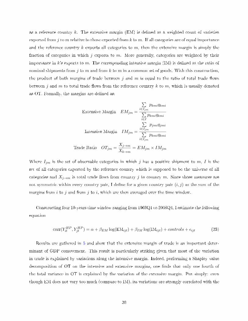
as a reference country k. The extensive margin (EM) is dened as a weighted count of varieties

exported from j tom relative to those exported from k tom. If all categories are of equal importance

and the reference country k exports all categories to m, then the extensive margin is simply the

fraction of categories in which j exports to m. More generally, categories are weighted by their

importance in k's exports to m. The corresponding intensive margin (IM) is dened as the ratio of

nominal shipments from j to m and from k to m in a common set of goods. With this construction,

the product of both margins of trade between j and m is equal to the ratio of total trade ows

between j and m to total trade ows from the reference country k to m, which is usually denoted

as OT. Formally, the margins are dened as:

Extensive Margin EMjm =

∑i∈Ijm

pkmiqkmi∑i∈I

pkmiqkmi

Intensive Margin IMjm =

∑i∈Ijm

pjmiqjmi∑i∈Ijm

pkmiqkmi

Trade Ratio OTjm =Xj→mXk→m

= EMjm × IMjm

Where Ijm is the set of observable categories in which j has a positive shipment to m, I is the

set of all categories exported by the reference country which is supposed to be the universe of all

categories and Xj→m is total trade ows from country j to country m. Since those measures are

not symmetric within every country-pair, I dene for a given country pair (i, j) as the sum of the

margins from i to j and from j to i, which are then averaged over the time window.

Constructing four 10-years time window ranging from 1969Q1 to 2008Q4, I estimate the following

equation

corr(Y HPit , Y HP

jt ) = α+ βEM log(EMijt) + βIM log(IMijt) + controls+ εijt (23)

Results are gathered in 5 and show that the extensive margin of trade is an important deter-

minant of GDP comovement. This result is particularly striking given that most of the variation

in trade is explained by variations along the intensive margin. Indeed, performing a Shapley value

decomposition of OT on the intensive and extensive margins, one nds that only one fourth of

the total variance in OT is explained by the variation of the extensive margin. Put simply: even

though EM does not vary too much (compare to IM), its variations are strongly correlated with the

30

variations of GDP comovement.41

dependent variable: corr(GDPHPi ,GDPHPj )

(1) (2) (3)

log(EM) 0.249*** 0.246*** 0.104

(8.91) (6.27) (1.91)

log(IM) 0.0111 0.120 0.023

(1.08) (0.45) (1.08)

Country-Pair FE no yes yes

Time FE no no yes

N 760 760 760

t stat. in parentheses, *** means p < 0.01, ** means p < 0.05 and *

means p < 0.10

Table 5: Strong Inuence of the Extensive Margin of trade

7.2 Terms of Trade and GDP: the role of Markups

Using data from 22 countries from 1971 to 2010,42 I assess the role of markups in generating a link

between terms of trade and GDP uctuations.

I test the following hypothesis: countries where markups are high experience a larger decrease

in GDP when experiencing an increase in their terms-of-trade. In order to test this hypothesis,

I compute the correlation of ltered GDP with the terms of trade and regress this correlation on

markups estimates. Results show that markups have a signicant impact on GDP-Terms of Trade

correlation, with higher markups associated with lower correlation between GDP and the terms of

trade.

Data on real GDP and terms of trade at the annual frequency are both taken from the OECD

database and ltered according to two dierent procedure. I rst apply the Hodrick and Prescott

lter with a smoothing parameter of 6.25 which captures the business cycle frequencies. I also

apply the Baxter and King band pass lter and keep uctuations between 8 and 25 years in order

to capture medium-term business cycles (Comin and Gertler (2006)). Using the detrended series,

I compute the correlation between ltered GDP and ltered terms-of-trade for two 20-years time

windows from 1971 to 2010, hence creating a panel dataset where each country appears two times.

41Those results are in line with the similar analysis in Liao and Santacreu (2015).42The list of countries is: Austria, Belgium, Canada, Denmark, Finland, France, Germany, Greece, Ireland, Iceland,

Israel, Italy, Japan, Korea, Luxembourg, Mexico, the Netherlands, Portugal, Spain, Sweden, the United-Kingdomand the United-States

31

I use Price Cost Margin (PCM) as an estimate of markups within each industry. Introduced by

Collins and Preston (1969) and widely used in the literature, PCM is the dierence between revenue

and variable cost, i.e. the sum of labor and material expenditures, over revenue:

PCM =Sales− Labor expenditure−Material expenditure

Sales(24)

Data at the industry level come from the OECD STAN database, an unbalanced panel covering

107 sectors for 34 countries between 1970 and 2010. Due to missing data for many countries in the

earliest years, I restrict the analysis for 22 countries.43 I compute PCM for each industry-country-

year and then construct an average of PCM within each country-year by taking the sales-weighted

average of PCM over each industry. Finally, the average PCM for a given time window is simply

the mean of country-year PCM over all time periods. Results are presented in table 6.

dependent variable: corr(GDP filteredi ,ToT filteredi )

HP-lter BK-lter HP-lter BK-lter

Average PCM -1.507*** -2.049*** -2.650*** -3.705***

(-2.70) (-3.11) (-2.87) (-4.10)

Country FE no no yes yes

Time FE no no yes yes

N 43

Note: The dependent variable is the correlation of ltered GDP with ToT. t stat. in

parentheses, *** means p < 0.01

Table 6: Markups and GDP-ToT correlation

The rst two columns of table 6 show the results of pooled cross-section analysis where I do not

use the panel dimension of the dataset. In the last two columns, I perform xed eect regression and

add time dummies to control for time specic factors that might aect the correlation of GDP and

terms-of-trade. In each of those cases, regressions are performed using the two ltering methods and

are found to be statistically signicant, implying that countries with higher markups also experience

a larger decrease in their GDP when the relative price of their import rises.

43For Germany, data are available only from 1991 onward (after the reunication), which is why the total numberof observation in the regressions is 43.

32

7.3 Trade and TFP comovement

The model predicts that in the presence of markups and extensive margin adjustment, a country's

TFP is impacted by foreign shocks even when technology is xed. As a result, trade proximity

across countries should be positively related to TFP correlation. I test this prediction using 18

OECD countries. Computing the correlation of all pairwise ltered TFP wihtin four 10-years time

window ranging from 1969Q1 to 2008Q4, I estimate the following equations:

(1) corr(TFP filteredit , TFP filteredjt ) = α1 + βT log(Totalijt) + controls+ ε1,ijt

(2) corr(TFP filteredit , TFP filteredjt ) = α2 + βI log(Intermediateijt) + βF log(Finalijt) + controls+ ε2,ijt

Results are presented in table 7 for the HP-ltered TFP, capturing the business cycle uctua-

tions and in table 8 for the BK-ltered TFP capturing medium run cycles. When using HP lter,

total trade is positively associated with TFP correlation, with trade in intermediate input capturing

all the statistical signicance in columns (2) and (4) while neither trade in intermediate nor nal

good is found signicant in column (6). The picture is clearer when studying the medium term

uctuation, as can be seen in table 8: trade in intermediate input captures all the statistical signi-

cance in columns (2), (4) and (6), leaving nal good trade with no explanatory power. Overall, this

analysis is more nuanced that when studying the relationship between trade and GDP comovement.

Nevertheless, it suggests that international trade is linked to TFP synchronization across countries

as predicted by the theory.

33

dependent variable: corr(TFPHPi ,TFPHPj )

(1) (2) (3) (4) (5) (6)

log(Total) 0.092*** 0.272*** 0.099**

(9.12) (11.05) (2.78)

log(Intermediate) 0.99*** 0.205*** 0.049

(4.47) (7.53) (1.45)

log(Final) -0.14 0.018 0.044

(-0.56) (0.44) (1.11)

Country-Pair FE no no yes yes yes yes

Time Trend no no no no yes yes

R-squared (within) 0.185 0.194 0.245 0.244

R-squared (overall) 0.118 0.128 0.120 0.130 0.213 0.217

N 612

t stat. in parentheses, *** means p < 0.01, ** means p < 0.05 and * means p < 0.10

Table 7: Relationship between Trade and HP ltered TFP correlation

dependent variable: corr(TFPBKi ,TFPBKj )

(1) (2) (3) (4) (5) (6)

log(Total) 0.091*** 0.296*** 0.079

(6.97) (9.58) (1.63)

log(Intermediate) 0.133*** 0.290*** 0.126**

(4.68) (8.55) (2.56)

log(Final) -0.53* -0.081 -0.054

(-1.66) (-1.48) (-1.00)

Country-Pair FE no no yes yes yes yes

Time Trend no no no no yes yes

R-squared (within) 0.140 0.172 0.201 0.207

R-squared (overall) 0.072 0.089 0.074 0.091 0.161 0.155

N 612

t stat. in parentheses, *** means p < 0.01, ** means p < 0.05 and * means p < 0.10

Table 8: Relationship between Trade and BK ltered TFP correlation

34

8 Conclusion

This paper analyzes the relationship between international trade and business cycle synchroniza-

tion across countries. I start by rening previous empirical studies and show that higher trade in

intermediate input is associated with an increase in GDP comovement, while trade in nal good is

found insignicant.

Motivated by this new fact, I propose a model of trade in intermediates with two key ingredients:

(1) monopolistic pricing and (2) rm entry/exit. Both elements are necessary in order for foreign

shocks to have a rst order impact on domestic productivity through trade linkages. The propagation

of technological shocks across countries depends on the worldwide network of input-output linkages,

which emphasize the importance of going beyond two-country models to understand international

GDP comovement.

I calibrate this model to 14 OECD countries and assess its ability to replicate the empirical nd-

ings. Overall, the quantitative exercise suggests that the model is able to replicate more than 70%

of the trade comovement slope, making an important step toward solving the Trade Comovement

Puzzle. Decomposing the role of each ingredient, I show that trade in intermediates alone is not

sucient to replicate the trade-comovement relationship. The addition of monopolistic pricing and

extensive margin adjustments increase the simulated trade-comovement slope by a factor seven.

References

[1] Anderson, J. E., and van Wincoop, E. Trade costs. Journal of Economic Literature 42,

3 (2004), 691751.

[2] Ansari, M. R. HUMMELS: Stata module to compute intensive and extensive trade margins.

Statistical Software Components, Boston College Department of Economics, Sept. 2013.

[3] Arkolakis, C., Costinot, A., and Rodriguez-Clare, A. New trade models, same old

gains? American Economic Review 102, 1 (2012), 94130.

[4] Arkolakis, C., and Ramanarayanan, A. Vertical specialization and international business

cycle synchronization*. The Scandinavian Journal of Economics 111, 4 (2009), 655680.

[5] Backus, D. K., Kehoe, P. J., and Kydland, F. E. International Real Business Cycles.

Journal of Political Economy 100, 4 (August 1992), 74575.

[6] Barrot, J.-N., and Sauvagnat, J. Input specicity and the propagation of idiosyncratic

shocks in production networks. Available at SSRN 2427421 (2014).

35

[7] Baxter, M., and Kouparitsas, M. A. Determinants of business cycle comovement: a

robust analysis. Journal of Monetary Economics 52, 1 (2005), 113157.

[8] Benassy, J.-P. Taste for variety and optimum production patterns in monopolistic competi-

tion. Economics Letters 52, 1 (July 1996), 4147.

[9] Bernard, A. B., Eaton, J., Jensen, J. B., and Kortum, S. Plants and productivity in

international trade. American Economic Review 93, 4 (2003), 12681290.

[10] Boehm, C., Flaaen, A., and Pandalai-Nayar, N. Input linkages and the transmission of

shocks: Firm-level evidence from the 2011 tohoku earthquake. Mimeo.

[11] Burstein, A., and Cravino, J. Measured aggregate gains from international trade. Amer-

ican Economic Journal: Macroeconomics 7, 2 (2015), 181218.

[12] Burstein, A., Kurz, C., and Tesar, L. Trade, production sharing, and the international

transmission of business cycles. Journal of Monetary Economics 55, 4 (2008), 775795.

[13] Calderon, C., Chong, A., and Stein, E. Trade intensity and business cycle synchroniza-

tion: Are developing countries any dierent? Journal of international Economics 71, 1 (2007),

221.

[14] Chaney, T. Distorted gravity: The intensive and extensive margins of international trade.

American Economic Review 98, 4 (2008), 170721.

[15] Chaney, T. The network structure of international trade. American Economic Review 104,

11 (2014), 36003634.

[16] Chetty, R., Guren, A., Manoli, D., and Weber, A. Are micro and macro labor supply

elasticities consistent? a review of evidence on the intensive and extensive margins. The

American Economic Review 101, 3 (2011), 471475.

[17] Comin, D., and Gertler, M. Medium-term business cycles. American Economic Review

96, 3 (2006), 523551.

[18] Di Giovanni, J., and Levchenko, A. A. Putting the parts together: Trade, vertical linkages,

and business cycle comovement. American Economic Journal: Macroeconomics 2, 2 (2010),

95124.

[19] Di Giovanni, J., and Levchenko, A. A. Firm entry, trade, and welfare in zipf's world.

Journal of International Economics 89, 2 (2013), 283296.

36

[20] Diewart, W. E., and Morrison, C. J. Adjusting Output and Productivity Indexes for

Changes in the Terms of Trade. Economic Journal 96, 383 (September 1986), 65979.

[21] Drozd, L. A., Kolbin, S., and Nosal, J. B. Long-run price elasticity of trade and the

trade-comovement puzzle. Working papers, Peruvian Economic Association, 2014.

[22] Drozd, L. A., and Nosal, J. B. Understanding International Prices: Customers as Capital.

American Economic Review 102, 1 (February 2012), 36495.

[23] Duval, R., Li, N., Saraf, R., and Seneviratne, D. Value-added trade and business cycle

synchronization. Journal of International Economics (2015), .

[24] Eaton, J., Eslava, M., Kugler, M., and Tybout, J. Export Dynamics in Colombia:Firm-

Level Evidence. Borradores de Economia 003957, Banco de la Republica, July 2007.

[25] Eaton, J., and Kortum, S. Technology in the Global Economy: A Framework for Quan-

titative Analysis. Unpublished Manuscript, New York University and University of Chicago.,

2005.

[26] Fattal Jaef, R. N., and Lopez, J. I. Entry, trade costs, and international business cycles.

Journal of International Economics 94, 2 (2014), 224238.

[27] Feenstra, R. C., and Jensen, J. B. Evaluating estimates of materials oshoring from u.s.

manufacturing. Economics Letters 117, 1 (2012), 170 173.

[28] Feenstra, R. C., Luck, P. A., Obstfeld, M., and Russ, K. N. In search of the armington

elasticity. Tech. rep., National Bureau of Economic Research, 2014.

[29] Feenstra, R. C., and Markusen, J. R. Accounting for Growth with New Inputs. Inter-

national Economic Review 35, 2 (May 1994), 42947.

[30] Frankel, J. A., and Rose, A. K. The Endogeneity of the Optimum Currency Area Criteria.

Economic Journal 108, 449 (July 1998), 100925.

[31] Ghironi, F., and Melitz, M. J. International trade and macroeconomic dynamics with

heterogeneous rms. The Quarterly Journal of Economics 120, 3 (2005), 865915.

[32] Gopinath, G., and Neiman, B. Trade adjustment and productivity in large crises. American

Economic Review 104, 3 (2014), 793831.

[33] Hummels, D., and Klenow, P. J. The variety and quality of a nation's exports. American

Economic Review 95, 3 (2005), 704723.

37

[34] Imbs, J. Trade, nance, specialization, and synchronization. Review of Economics and Statis-

tics 86, 3 (2004), 723734.

[35] Inklaar, R., Jong-A-Pin, R., and De Haan, J. Trade and business cycle synchronization

in oecd countries: A re-examination. European Economic Review 52, 4 (2008), 646666.

[36] Johnson, R. C. Trade in intermediate inputs and business cycle comovement. American

Economic Journal: Macroeconomics 6, 4 (2014), 3983.

[37] Jones, C. I. Intermediate goods and weak links in the theory of economic development.

American Economic Journal: Macroeconomics 3, 2 (2011), 128.

[38] Juarez, F. C. SHAPLEY2: Stata module to compute additive decomposition of estimation

statistics by regressors or groups of regressors. Statistical Software Components, Boston College

Department of Economics, Nov. 2012.

[39] Kehoe, T. J., and Ruhl, K. J. Are shocks to the terms of trade shocks to productivity?

Review of Economic Dynamics 11, 4 (2008), 804 819.

[40] Kennan, J. Uniqueness of positive xed points for increasing concave functions on rn: An

elementary result. Review of Economic Dynamics 4, 4 (2001), 893 899.

[41] Kim, S. T. The Price of Imports and TFP: Application to the Korean Crisis of 1997-98. Review

of Economic Dynamics 17, 1 (January 2014), 3951.

[42] Kose, M. A., and Yi, K.-M. Can the standard international business cycle model explain

the relation between trade and comovement? Journal of international Economics 68, 2 (2006),

267295.

[43] Lawless, M. Firm export dynamics and the geography of trade. Journal of International

Economics 77, 2 (April 2009), 245254.

[44] Liao, W., and Santacreu, A. M. The trade comovement puzzle and the margins of inter-

national trade. Journal of International Economics 96, 2 (2015), 266 288.

[45] Llosa, L.-G. How Do Terms of Trade Aect Productivity? The Role of Monopolistic Output

Markets. Working Papers 2014-7, Peruvian Economic Association, Feb. 2014.

[46] Melitz, M. J. The impact of trade on intra-industry reallocations and aggregate industry

productivity. Econometrica 71, 6 (2003), 16951725.

38

[47] Ng, E. C. Production fragmentation and business-cycle comovement. Journal of International

Economics 82, 1 (2010), 114.

[48] Saito, M. Armington elasticities in intermediate inputs trade: a problem in using multilateral

trade data. Canadian Journal of Economics 37, 4 (November 2004), 10971117.

39

A Empirical Appendix

A.1 Data description

I focus the empirical analysis on a subset of all OECD countries. For the evolution of GDP cor-

relation, I use 24 countries for which I could gather quarterly data on real GDP, which gives me

N(N − 1)/2 = 276 country pairs. Those are Australia, Austria, Belgium, Canada, Denmark, Fin-

land, France, Germany, Ireland, Italy, Japan, Luxembourg, Mexico, Netherlands, New-Zealand,

Norway, Portugal, South-Africa, Spain, Sweden, Switzerland, Turkey, the United Kingdom and the

United States. For the study of the trade-comovement, I took out four countries from the sample.

I get rid of Belgium and Luxembourg because they were pooled together in the trade data until

the year 2000, preventing me from using 4 time windows and perform the xed eect regression

properly. I also took out New Zealand and South Africa because their trade data contained many

zeros for some time periods,44 resulting in some country-pairs being presents only for some time

windows and hence reducing the eectiveness of the xed eect regression. This leaves me in the

end with 20 countries, so 190 country pairs for each of the four time window.

I use data from the OECD database VPVOBARSA which features quarterly GDP. In this

database, GDP is constructed with volume estimates and with constant 2005 prices. As for the

trade ows, I use two datasets. From 1968 to 1999, I use the NBER-UN world trade data updated

on the 30th of January, 2009.45 From 2000 onward, I use the revision of those data. In both datasets,

trade ows are categorized using SITC4, which represents the rst 4 digits of the SITC Rev 2 cat-

egorization. I follow Feenstra and Jensen (2012) to separate nal from intermediate goods. First, I

translate the SITC4 codes into END USE codes using the concordance table available on the CID

website.46 The end-use codes are used by the Bureau of Economic Analysis to allocate goods to their

nal use, within the National Income and Product Accounts. I then label as intermediate goods

the products which end-use codes correspond to the list put together by Feenstra and Jensen (2012).

44To x ideas, in 1969, while Spain was importing from 134 countries and exporting to 140 countries, South Africawas importing from only 65 and exporting to 77 countries. As for New Zealand, the numbers were 105 (imports) and127 (exports).

45This data is constructed from United Nations trade data by Robert Feenstra and Robert Lipsey. It can bedownloaded, as well as the associated documentation, from the Center for International Data (CID)'s website athttp://cid.econ.ucdavis.edu/nberus.html

46See at http://cid.econ.ucdavis.edu/usix.html, under the directory 1972-2006 U.S. import data - SAS andSTATA.

40

A.2 Robustness Checks and other results

A.2.1 Changing the Dataset

As a robustness check, I also use the STAN Bilateral Trade Database by Industry and End-Use data

(BTDIxE).47 BTDIxE consists of values of imports and exports of goods, broken down by end-use

categories. Estimates are expressed in nominal terms, in current US dollars for all OECD member

countries. The trade ows are divided into capital goods, intermediate inputs and consumption. For

the sake of comparison with the results in the main text, I rst group the capital and intermediate

goods together and create the index of trade proximity as explained in the main text. Due to data

availability, I use the data from 1995 to 2014 which allows me to create four time windows of 5

years each (tables 9 and 10). With 20 countries, the dataset contains 190 pairs, for a total of 760

observations with four time windows. The tables below present the robustness results using both

the HP lter (for business cycle frequencies) and then the Baxter and King lter (for medium term

frequencies).

dependent variable: corr(GDPHPi ,GDPHPj )

(1) (2) (3) (4) (5) (6)

log(Total) 0.064*** -0.009 0.103

(5.94) (-0.14) (1.53)

log(Intermediate) 0.044* 0.146* 0.209***

(1.88) (1.77) (2.59)

log(Final) 0.021 -0.152* -0.107

(1.06) (-2.04) (-1.39)

Country-Pair FE no no yes yes yes yes

Time Trend no no no no yes yes

N 760

t stat. in parentheses, *** means p < 0.01, ** means p < 0.05 and * means p < 0.10

Table 9: Trade and HP-Filtered GDP - STAN database (1995 to 2014)47See at http://www.oecd.org/trade/bilateraltradeingoodsbyindustryandend-usecategory.htm.

41

dependent variable: corr(GDPBKi ,GDPBKj )

(1) (2) (3) (4) (5) (6)

log(Total) 0.075*** 0.433*** 0.397***

(5.23) (3.86) (3.16)

log(Intermediate) 0.115*** 0.562*** 0.538***

(3.71) (3.71) (3.60)

log(Final) -0.036 -0.106 -0.122

(-1.32) (-0.76) (-0.83)

Country-Pair FE no no yes yes yes yes

Time Trend no no no no yes yes

N 760

t stat. in parentheses, *** means p < 0.01, ** means p < 0.05 and * means p < 0.10

Table 10: Trade and BK-Filtered GDP - STAN database (1995 to 2014)

A.2.2 Separating Intermediate goods from Capital goods

In the OECD STAN database, one can separate intermediate goods from capital goods. I use this

categorization and perform the same empirical exercise as above.

42

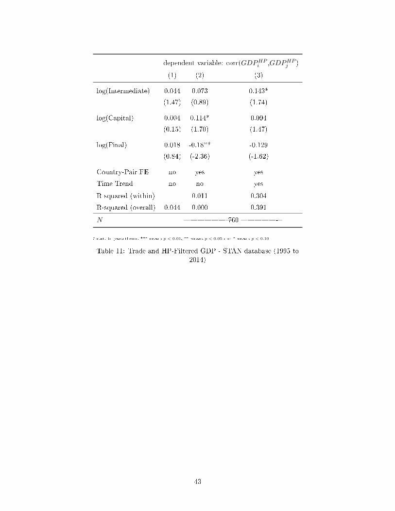
dependent variable: corr(GDPHPi ,GDPHPj )

(1) (2) (3)

log(Intermediate) 0.044 0.073 0.143*

(1.47) (0.89) (1.74)

log(Capital) 0.004 0.114* 0.094

(0.15) (1.70) (1.47)

log(Final) 0.018 -0.18** -0.129

(0.84) (-2.36) (-1.62)

Country-Pair FE no yes yes

Time Trend no no yes

R-squared (within) 0.011 0.304

R-squared (overall) 0.044 0.000 0.391

N 760 -

t stat. in parentheses, *** means p < 0.01, ** means p < 0.05 and * means p < 0.10

Table 11: Trade and HP-Filtered GDP - STAN database (1995 to2014)

43

dependent variable: corr(GDPBKi ,GDPBKj )

(1) (2) (3)

log(Intermediate) 0.024 0.449*** 0.420***

(0.62) (3.05) (2.95)

log(Capital) 0.112*** 0.150 0.158

(2.95 ) (1.37) (1.42)

log(Final) -0.053* -0.132 -0.153

(-1.88 ) (-0.96) (-1.04)

Country-Pair FE no yes yes

Time Trend no no yes

R-squared (within) 0.057 0.059

R-squared (overall) 0.045 0.042 0.044

N 760 -

t stat. in parentheses, *** means p < 0.01, ** means p < 0.05 and * means p < 0.10

Table 12: Trade and BK-Filtered GDP - STAN database (1995 to2014)

A.3 Evolution of GDP correlation

In the graph below, I use a sample of 24 OECD countries from 1960 to 2012 and compute the

GDP correlation for all pair of countries using a 10 years rolling window. Each point of this graph

represents the average correlation of GDP across all country-pair in the 10 years preceding the point.

The vertical red line is set at 2007Q3 and is a rough materialization of the last nancial crisis. The

point which is exactly at the red line is then the average GDP correlation from 1997Q3 to 2007Q3

and hence is not aected by the collapse of subprime markets and the events that followed. The

graph on the left is the correlation HP ltered in order to keep the business cycle frequency, while

on the right I used the Baxter and King lter to extract uctuations from 32 to 200 quarters as

suggested by Comin and Gertler (2006).

44

B Theoretical Appendix

B.1 Equilibrium Conditions in the general CES case

Price Indexes and Pricing System

Pk,k′ =

∫Ωk,k′

pk,k′(ϕ)1−σg(ϕ)dϕ

1

1−σ

and IPk =

∑k′=1,...,N

ωk(k′)P1−ρ

k′,k

11−ρ

PBk = χ−χkk × η−ηkk × (1− ηk − χk)(ηk+χk−1) × IP 1−ηk−χkk × wχkk × r

ηkk

Using the optimal pricing strategy pk,k′ = τk,k′σσ−1

PBkZkϕ

with the denition of the price index relative

to each country specic bundle, we have the pricing system:

P1−ρk = µk

∑k′

ωk(k′)

(τk′k

(ϕk′,kϕk′,k′

)σ−γ−11−σ

Pk′)1−ρ1−ηk−χk

, k = 1, ..., N

with µ1−σ1−ρk =

γϕσ−γ−1k,k

γ−(σ−1)Mk

(σσ−1

wχkk ×r

ηkk

χχkk ×η

ηkk ×(1−ηk−χk)1−ηk−χk

1Zk

)1−σ.

Entry Thresholds

In very market, entry occurs until the prot of the least productive rms is equal to the xed cost of

accessing the market. Denoting by Xk total nal good spending by consumers (Xk = Pk(Ck+Ik) =

wkLk + rkKk + Πk), we get

45

At Home

πk,k(ϕk,k) = fk,kPBkZk

⇔ ϕk,k =

(σ

σ − 1

PBkZk

1

Pk

)×

σfk,kPBkZk

Xk +(PkIPk

)1−ρωk(k)(1− ηk − χk)Sk

1

σ−1

Abroad

πk,k′(ϕk,k′) = fk,k′PBkZk

⇔ ϕk,k′ =

(τkk′

σ

σ − 1

PBkZk

1

Pk,k′

)×

σfk,kPBkZk(Pk,k′

IPk′

)1−ρωk′(k)(1− ηk − χk)Sk′

1

σ−1

Replacing Pk,k′ by its expression using Pk, we also get

ϕ1+

(γ−(σ−1)).(σ−ρ)(σ−1)2

k,k′ =

(τρ−1σ−1

kk′σ

σ − 1

PBkZk

IP1−ρσ−1

k′

(ϕσ−γ−1σ−1

k,k .Pk) ρ−σσ−1

)×

(σfk,k′

PBkZk

ωk′(k)(1− ηk − χk)Sk′

) 1σ−1

Spending System

Total revenue of all rms from country k can be written as

Rk = Xk +

[∑k′

(Pk,k′IPk′

)1−ρωk′(k)(1− ηk − χk)Sk′

]

Free entry insures that variable prots are exactly equal, on aggregate, to xed costs and entry costs

payment, implying thatRk = Sk. Capital and labor demand impose rkKk+wkLk = (ηk+χk)Sk+Πk.

Finally, the spending system can be simply written as(IN −

(W T P

))︸ ︷︷ ︸=M

S1

...

SN

= 0RN

whereW the weighting matrix dened asWij = ωi(j), P a matrix dened by Pij =(Pi,jIPi

)1−ρand

is the element-wise (Hadamard) product. One can easily show that the matrixM is non invertible48

and is of rank exactly N − 1, meaning that the solutions of the system is a one dimensional space.

48One can easily see that summing all rows results in a column of zero.

46

This is reassuring because it means we can normalize one price to one. I then normalize w1 = 1

and with the labor demand equation this results is

S1 =L1

χ1

Labor and Capital Market Equilibrium

Using the labor supply equation, Lk is simply

Lνk =1

ψk

wkPk

Equipped with Sk the total spending of all rms in k, wages wk and rental rate rk are dened simply

by

wk = χkSkLk

and rk = ηkSkKk

Free Entry

At each date, rms enter the model until total prots are equal to total sunk cost payment:

Πk = MkPBkZk

.fE,k for all k

B.2 Proof of Lemma 1

Reminder of Lemma 1 : Total prot in country k are proportional to total revenues:

Πk =σ − 1

γσRk

Proof

First, since rms charge a constant markup σ/(σ − 1) over marginal cost, we know that variable

prots are a fraction 1/σ of total revenues. Hence, total prots net of xed costs for all rms in k

are simply

Πk =Rkσ−∑k′

FCk→k′

47

where FCk→k′ is the sum of xed cost payment from all rms from country k serving market k′.

Then, note that total xed cost payment for all rms in country k is

FCk→k′ = Mk

+∞∫ϕk,k′

fkk′ ×PBkZk× γϕ−γ−1 × dϕ

= Mkfkk′PBkZk× ϕ−γk,k′

If k 6= k′, we can also express total revenues (sales) from k to k′ as

Rk,k′ = Mk

+∞∫ϕk,k′

(τkk′

σ

σ − 1

PBkZk

1

Pk,k′

)1−σ× ωk′(k)Sk′ϕ

σ−1g(ϕ)dϕ

=γMk

γ − (σ − 1)×(τkk′

σ

σ − 1

PBkZk

1

Pk,k′

)1−σ× ωk′(k)Sk′ϕ

σ−γ−1k,k′

Next, using the expression for the threshold ϕσ−1k,k′ derived above (as a function of Pk,k′), we

get

Rk,k′ =γMk

γ − (σ − 1)× σfk,k′

PBkZk

ϕ−γk,k′

And we recognize nally that

Rk,k′ =γ

γ − (σ − 1)× σFCk→k′

For domestic revenues, we can show using the same steps that

Xk +Rk,k =γ

γ − (σ − 1)× σFCk→k

Combining those expressions, we get

∑k′

FCk→k′ =γ − (σ − 1)

γσ×

(Xk +

∑k′

Rk,k′

)

=γ − (σ − 1)

γσ×Rk

Using this expression of∑k′FCk→k′ in the denition of prots completes the proof.

48

B.3 Proof of Lemma 2

Reminder of Lemma 2 : In the Cobb-Douglas (ρ = 1) and xed labor supply case, the elasticity

of every GNI with respect to a technology shock in country 1 is given by:ηGNI1,Z1

...

ηGNIN ,Z1

= (IN − (1− ηk − χk)W − T )−1

1

0...

with W the weighting matrix dened above and T a Transmission matrix function of γ and σ.

Proof:

In this simplied case (ρ = 1 and xed labor and capital supply), the labor and capital demand

schedules wkLk = χkSk and rkKk = ηkSk provide a one to one mapping between total spendings

Sk and the wages wk and the interest rate rk. Moreover, inspecting the spending system (18)

when ρ = 1 reveals that once a choice of numeraire is done (that is, taking w1 = 1 and hence

xing S1 = L1/χ1), the vector of spendings (Si)i=1,...,N is independent of the technology level.

Using lemma 1 and the fact that labor and capital supply are xed, we can then show that total

consumers' spending Xi also independent of technology level. Thus, since GNIk = Xk/Pk the GNI

elasticity is simply the opposite of the elasticity of the country's consumers price index. Moreover,

with xed labor supply and the assumption that the mass of potential entrepreneurs is proportional

to labor size, the mass of rms Mi is xed for every country i. In the next sections, I compute

elasticities of all endogenous variables step by step until I can solve for the price index elasticities.

B.3.1 Model-based Price Indexes

Home Price Index at home PkUsing the denitions of price indexes, we can easily show that

∂ log(Pk)∂ log(Zk)

= −1 +∂ log(PBk)

∂ log(Zk)+

(γ − (σ − 1)

σ − 1

)∂ log(ϕk,k)

∂ log(Zk)

We can see in this formula the direct eect of lowering all prices in country k plus two other indirect

eects : the propagation going through the input-output linkages in the PBk term as well as the

extensive margin of entry of new rms through the ϕk,k term.

49

Foreign Price Index at their home Pk′

∂ log(Pk′)∂ log(Zk)

=∂ log(PBk′)

∂ log(Zk)+

(γ − (σ − 1)

σ − 1

)∂ log(ϕk′,k′)

∂ log(Zk)

The foreign price index at their home is not aected directly but only through the eects going

through the input output linkages as well as the entry of new rms.

Export Price indexes Pi,jThe price index relative to varieties from i sold on j's market is aected by the shock according to:

∂ log(Pi,j)∂ log(Zk)

=∂ log(Pi)∂ log(Zk)

+

(γ − (σ − 1)

σ − 1

)(∂ log(ϕi,j)

∂ log(Zk)− ∂ log(ϕi,i)

∂ log(Zk)

)We can see that the eect of a technology shock on exporting price indexes depends on the widening

in the range of exported goods, as measured by the second term, in the brackets.

Input Bundle Price PBk′ Abroad

Using the fact that wages are not aected by technology shocks, I can compute the elasticity of the

input bundle price with respect to a technology shock at home as follow:

∂ log(PBk′)

∂ log(Zk)= (1− ηk − χk)

∑j

ωk′(j)

[∂ log(Pj)∂ log(Zk)

+

(γ − (σ − 1)

σ − 1

)(∂ log(ϕj,k′)

∂ log(Zk)− ∂ log(ϕj,j)

∂ log(Zk)

)]

B.3.2 Thresholds

Home Entry Threshold ϕk,k at Home

Using the denition of the thresholds from above and replacing ∂ log(PBk)∂ log(Zk) − 1 by its expression in

the expression of the elasticity of the Home price index at home, we get

∂ log(ϕk,k)

∂ log(Zk)=

1

σ − 1 + κσ× ∂ log(Pk)∂ log(Zk)

The scaling factor ( 1σ−1+κσ ) is positive while the second term is negative, meaning that a positive

technology shock trigers the entry of more rms in the country, which amplies the eect of the

shock.

Export Entry Threshold ϕk,k′ for Home rms exporting to k′

Using the second denition of the export thresholds from above, we get

(γ

σ − 1)∂ log(ϕk,k′)

∂ log(Zk)= (1 +

1

σ − 1)×

(∂ log(PBk)

∂ log(Zk)− 1

)+ κ

∂ log(ϕk,k)

∂ log(Zk)− ∂ log(Pk)∂ log(Zk)

50

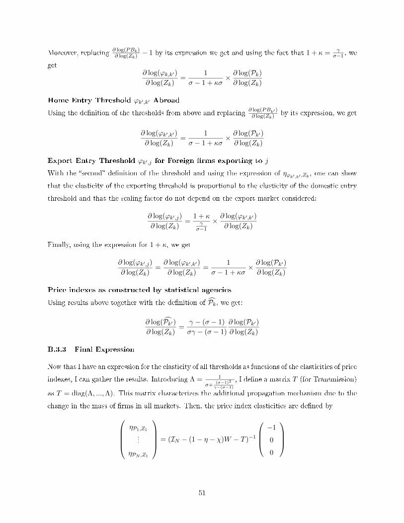
Moreover, replacing ∂ log(PBk)∂ log(Zk) − 1 by its expression we get and using the fact that 1 + κ = γ

σ−1 , we

get∂ log(ϕk,k′)

∂ log(Zk)=

1

σ − 1 + κσ× ∂ log(Pk)∂ log(Zk)

Home Entry Threshold ϕk′,k′ Abroad

Using the denition of the thresholds from above and replacing∂ log(PBk′ )∂ log(Zk) by its expression, we get

∂ log(ϕk′,k′)

∂ log(Zk)=

1

σ − 1 + κσ× ∂ log(Pk′)∂ log(Zk)

Export Entry Threshold ϕk′,j for Foreign rms exporting to j

With the second denition of the threshold and using the expression of ηϕk′,k′ ,Zk , one can show

that the elasticity of the exporting threshold is proportional to the elasticity of the domestic entry

threshold and that the scaling factor do not depend on the export market considered:

∂ log(ϕk′,j)

∂ log(Zk)=

1 + κγ

σ−1

×∂ log(ϕk′,k′)

∂ log(Zk)

Finally, using the expression for 1 + κ, we get

∂ log(ϕk′,j)

∂ log(Zk)=∂ log(ϕk′,k′)

∂ log(Zk)=

1

σ − 1 + κσ× ∂ log(Pk′)∂ log(Zk)

Price indexes as constructed by statistical agencies

Using results above together with the denition of Pk, we get:

∂ log(Pk′)∂ log(Zk)

=γ − (σ − 1)

σγ − (σ − 1)

∂ log(Pk′)∂ log(Zk)

B.3.3 Final Expression

Now that I have an expression for the elasticity of all thresholds as functions of the elasticities of price

indexes, I can gather the results. Introducing Λ = 1

σ+(σ−1)2

γ−(σ−1)

, I dene a matrix T (for Transmission)

as T = diag(Λ, ...,Λ). This matrix characterizes the additional propagation mechanism due to the

change in the mass of rms in all markets. Then, the price index elasticities are dened byηP1,Z1

...

ηPN ,Z1

= (IN − (1− η − χ)W − T )−1

−1

0

0

51

Finally, noting that for all i, ηPi,Z1 = −ηGNIi,Z1 concludes the demonstration.

In order to gain intuition on this formula, a few comments are in order. First, note that in the case

of complete autarky of all countries we have W = IN to that the elasticity for country 1 is simply

ηGNI1,Z1 = 1/(η1 +χ1−Λ) whereas all other elasticities are zero. This result is reminiscent of what

is found in Jones (2011) with the additional propagation mechanism due to the adjustment along

the extensive margin captured by Λ. Interestingly, this special case highlights the fact that we need

(1− η−χ) + Λ < 1 in order to get a positive own-country elasticity. This condition is necessary for

the validity of (21), since it corresponds to imposing that the reason of the geometric sequence is

below one.49 Secondly, noting that Λ = 1

σ+(σ−1)2

γ−(σ−1)

, one can see that for a xed σ, Λ(γ) is a strictly

increasing function. When γ → σ−1, Λ→ 0 and when γ → +∞, Λ→ 1/σ. For a labor and capital

share so that η+χ = 0.7 we can see that any value σ > 1.5 is sucient to insure the validity of the

condition (1− η − χ) + Λ < 1 for any value of γ within the range of admissible values (γ > σ − 1).

49The formula (21) is the matrix analogue of summing an innite geometric sequence. (1−η−χ)W+T correspondsto the rst order eect of the shock, ((1− η − χ)W + T )2 is the second order eect, etc... The total eect can thenbe described by the matrix (IN − (1− η−χ)W − T )−1 if and only if the eigenvalues of the matrix (1− η−χ)W + Tall lie within the unit circle. In the autarcy case, this condition is insured by (1− η − χ) + Λ < 1.

52