University of Minnesota

Department of Economics

Revised April 2016

Intangible Capital and Measured Productivity

Ellen R. McGrattan

University of Minnesota

and Federal Reserve Bank of Minneapolis∗

ABSTRACT

Because firms invest heavily in R&D, software, brands, and other intangible assets—at a rate closeto that of tangible assets—changes in measured GDP, which does not include all intangible in-vestments, understate the actual changes in total output. If changes in the labor input are moreprecisely measured, then it is possible to observe little change in measured total factor productivity(TFP) coincidentally with large changes in hours and investment. This mismeasurement leavesbusiness cycle modelers with large and unexplained labor wedges accounting for most of the fluc-tuations in aggregate data. In this paper, I incorporate intangible investments into a multi-sectorgeneral equilibrium model and parameterize income and cost shares using data from the U.S. inputand output tables, with intangible investments added to final goods and services. I use maximumlikelihood methods and observations on sectoral gross outputs and per capita hours for the period1948–2014 to estimate processes for latent sectoral TFPs—that have common and idiosyncraticcomponents—and a time-varying labor wedge. I find that neither a large and unexplained laborwedge nor a large common TFP shock is needed to account for fluctuations in these data.

∗ The views expressed herein are those of the authors and not necessarily those of the Federal Reserve Bank of

Minneapolis or the Federal Reserve System.

1. Introduction

This paper sheds light on a measurement issue that confounds analyses of key macrodata

during economic booms and busts. Because firms invest heavily in R&D, software, brands, and

other intangible assets—at a rate close to that of tangible assets—changes in GDP, which does

not include all intangible investments, understate the actual changes in total output. As a result,

it is possible to observe large changes in hours and investment coincidentally with little change

in measured total factor productivity. In other words, innovation by firms—which is fueled in

large part by their intangible investments—may be evident “everywhere but in the productivity

statistics.”1

Here, I use a dynamic multi-sector general equilibrium model and U.S. data from the Bureau

of Economic Analysis (BEA) to quantify the impact of updating both theory and the national

accounts to include intangible investment. Multiple sectors are included to account for the vast

heterogeneity in intangible investment rates across industries. I start with the BEA’s 2007 bench-

mark input-output table, that now includes expenditures on software, R&D, mineral exploration,

entertainment, literary, and artistic originals as part of investment rather than as part of inter-

mediate inputs. I additionally reallocate several categories of intermediate inputs that are under

consideration for future inclusion in the BEA fixed assets including computer design services, ar-

chitectural and engineering services, management consulting services, advertising, and marketing

research. The revised input and output table is then used to parameterize the model’s income

and cost shares. From the BEA, I have gross output by industry, which are used to estimate

stochastic processes of shocks impacting sector-specific and aggregate total factor productivity.2

Because the model includes intangible investments, I cannot directly measure industry or aggre-

gate TFP series as has been done in earlier work. (See, for example, Horvath (2000).) Instead, I

use maximum likelihood methods to estimate stochastic processes for TFPs—that are assumed to

have both sector-specific components and a common component. The estimates can then be used

to construct predictions of the model’s latent productivity shocks.

Because earlier work finds that a large and unexplained labor wedge is needed to account for

1 Solow (1987) remarked that the computer age could be seen everywhere but in the economic data.2 I also worked with IRS business receipts, which are an important source of information for constructing gross

outputs and are available back to the 1920s for many major and minor industries.

2

observed business cycles, I also include a time-varying wedge as a potential source of fluctuations.

(See Chari et al. (2007, 2016).) This wedge, which stands in for unmodeled factors impacting

households’ labor-leisure decisions, is treated as an exogenous process and serves as a check on

the overall model specification. The TFP processes are not correlated with the labor wedge but

can be correlated across sectors. I consider two specifications. In the first, I do not restrict the

variance-covariance matrix for the sectoral TFP shocks, thus allowing for a common component to

have some impact. In the second, I assume that sectoral shocks are the sum of two autoregressive

processes: one that is sector-specific and one that is common. The latter specification is restrictive,

but is more informative about the role of input-output linkages.

Using data for the period 1948–2014, I find that neither a large and unexplained labor wedge

nor a large common TFP shock is needed to account for business cycle fluctuations in U.S. gross

output by sector or hours per capita.3 The main sources of the fluctuations for all observables

are the sectoral TFP shocks, and industry linkages play an important role in generating realistic

cycles. Although I cannot directly measure the sectoral TFPs, I can use the model predictions to

infer these latent series. When I compute correlations between these series and typical measures

of productivity, such as the aggregate Solow residual or GDP per hour, I find them to be weakly

positive or negative for most sectors. Part of the reason for this is the fact that the observed gross

output series are not highly correlated with the Solow residual or GDP per hour, especially in the

latter part of my sample.

Previous theoretical work related to this paper has either abstracted from intangible capital

or been more limited in scope. Long and Plosser (1983) analyzed a relatively simple multi-sector

model, arguing that firm- and industry-level shocks could generate aggregate fluctuations. Horvath

(1998, 2000) and Dupor (1998) extended their model and studied the nature of industry linkages to

determine if independent productivity shocks could in fact generate much variation for aggregate

variables. Parameterizing the model to match the input-output and capital-use tables for the 1977

BEA benchmark, Horvath (2000) concludes that sectoral shocks may have significant aggregate

effects, but he does not compute the model’s variance decomposition. More recently, Foerster,

3 The small role for a common TFP shock relies importantly on assuming that TFP shocks in the governmentindustry (NAICS 92) are independent of other industry shocks.

3

Sarte, and Watson (2011) do a full structural factor analysis of the errors from the same multi-

sector model, but only use data for sectors within manufacturing and mining. Neither Horvath

(2000) nor Foerster et al. (2011) distinguish tangible and intangible investments. McGrattan and

Prescott (2010) do distinguish the different investments, but focus only on aggregate data for a

specific episode, namely the technology boom of the 1990s.

Previous empirical work has documented that intangible investments are large and vary with

tangible investments over the business cycle. For example, Corrado, Hulten, and Sichel (2005,

2006) estimate that intangible investments made by businesses are about as large as their tangi-

ble investments.4 McGrattan and Prescott (2014) use firm-level data and show that intangible

investments are highly correlated with tangible investments like plant and equipment.

The model is described in Section 2. Parameters of the model are described in Section 3.

Section 4 summarizes the results. Section 5 concludes.

2. Model

There is a stand-in household that supplies labor to competitive firms and, as owners of the

firms, receives the dividends. There is a government with certain spending obligations that are

financed by various taxes on households and firms. Firms produce final goods for households and

the government and intermediate inputs for other firms. The sources of fluctuations in the economy

are stochastic shocks to firm productivities.5

There are J sectors in the economy. Firms in sector j maximize the present value of dividends

Djt paid to their shareholders. I assume that firms in each sector j produce both tangible goods

and services, Yj , and intangible intangible investment goods and services, XIj . The technologies

available are as follows:

Yjt =(

K1Tjt

)θj(KIjt)

φj

(

∏

l

(

M1ljt

)γlj

)

(

Z1jtH

1jt

)1−θj−φj−γj(2.1)

4 For more details on measurement of intangible investments in the national accounts, see recent surveys inthe BEA’s Survey of Current Business (U.S. Department of Commerce, 1929–2013). For more details onmeasurement of R&D investments, see National Science Foundation (1953–2013). For details on entertainment,literary, and artistic originals, see Soloveichik and David Wasshausen (2013).

5 Later, I plan to include shocks to government spending and to tax rates.

4

XIjt =(

K2Tjt

)θj(KIjt)

φj

(

∏

l

(

M2ljt

)γlj

)

(

Z2jtH

2jt

)1−θj−φj−γj(2.2)

and depend on inputs of tangible capital K1Tj , K

2Tj , intangible capital KIj , intermediate inputs

M1ljt, M

2ljt, and hours H1

j , H2j . These production technologies are hit by stochastic technology

shocks, Z1jt and Z2

jt, that could have a common component and sector-specific components. The

specific choices for the stochastic processes are discussed below.

Firms in sector j maximize the present value of after-tax dividends on behalf of their owners

(households) that discount after-tax future earnings at the rate ρt:

max E0

∞∑

t=0

(1 − τdt) ρtDjt,

where

Djt = PjtYjt +QjtXIjt −WjtHjt −∑

l

PltMljt −∑

l

PltXTljt −∑

l

QltXIljt

− τktPjtKTjt − τxt∑

l

PltXTljt

− τptPjtYjt +QjtXIjt −WjtHjt − (δT + τkt)PjtKTjt

−∑

l

PltMljt −∑

l

QltXIljt (2.3)

KTjt+1 = (1 − δT )KTjt +∏

l

Xζlj

Tljt (2.4)

KIjt+1 = (1 − δI)KIjt +∏

l

Xνlj

Iljt (2.5)

Mljt = M1ljt +M2

ljt. (2.6)

Dividends are equal to gross output PjYj+QjXIj less wage payments to workers WjHj , purchased

intermediate goods∑

l PlMlj , new tangible investments∑

l PlXTlj , new intangible investments

∑

lQlXIlj , and taxes. New investment goods and services are purchased from other sectors and

used to update capital stocks as in (2.4) and (2.5). Taxes are levied on property at rate τkt,

investment at rate τxt (which could be negative if it is an investment tax credit), and accounting

profits at rate τpt.

Households choose consumption Ct and leisure Lt to maximize expected utility:

max E0

∞∑

t=0

βt

[

(Ct/Nt) (Lt/Nt)ψ]1−α

− 1

/ (1 − α)Nt (2.7)

5

with the population equal to Nt = N0(1 + gn)t. The maximization is subject to the following

per-period budget constraint:

(1 + τct)J∑

j=1

[PjtCjt + Vjt (Sjt+1 − Sjt)]

≤ (1 − τht)J∑

j=1

WjtHjt + (1 − τdt)J∑

j=1

DjtSjt + Ψt, (2.8)

where Cjt is consumption of goods made by firms in sector j which are purchased at price Pjt, Hjt

is labor supplied to sector j which is paid Wjt, and Djt are dividends paid to the owners of firms

in sector j who have Sjt outstanding shares that sell at price Vjt. Taxes are paid on consumption

purchases (τct), labor earnings (τht) and dividends (τdt). Any revenues in excess of government

purchases of goods and services are lump-sum rebated to the household in the amount Ψt.

The composite consumption and leisure that enter the utility function are given by

Ct =

∑

j

ωjCσ−1

σ

jt

σσ−1

(2.9)

Lt = Nt −∑

j

Hjt. (2.10)

Notice that here, I assume CES for consumption and linear for hours. As owners of the firm, the

household’s discount factor is the relevant measure for ρt in (2.3):

ρt = βtUct/ [Pt (1 + τct)] . (2.11)

The resource constraints for tangible and intangible goods and services are given as follows:

Yjt = Cjt +∑

l

XTjlt +∑

l

Mjlt +Gjt (2.12)

XIjt =∑

l

XIjlt, (2.13)

where Yj and XIj are defined in (2.1) and (2.2), respectively. The model economy is closed and,

therefore, there is no term for net exports.

Two specifications are considered for the sectoral TFP stochastic processes. In the first,

logZijt = ςij logZijt−1 + ηijt,

6

with mean zero, serially uncorrelated errors that are correlated across sectors, that is, Eηijt = 0,

Eηijtηijt−1 = 0, and Eηijtη

klt 6= 0 for all i, j, k, l. I call this the specification of the model with an

unrestricted variance-covariance matrix. For the second specification, I assume that the logs of

the sectoral TFP processes are equal to the sum of a sector-specific component Zijt and a common

component Zt, namely,

logZijt = log Zijt + logZt (2.14)

log Zijt = ςij log Zijt−1 + ηijt (2.15)

logZt = ς logZt−1 + υt, (2.16)

with Eηijt = 0, Eηijtηijt−1 = 0, Eηijtη

klt = 0 for all i, j, k, l except cases with j = l, Eυt = 0,

Eυtυt−1 = 0, and Eυtηijt = 0. In other words, the shocks to TFP are correlated within a sector

but not across sectors and not with the common TFP component.6 I call this the specification of

the model with a restricted variance-covariance matrix.

An approximate equilibrium for the model economy can be found by applying a version of

Vaughan’s (1970) method to the log-linearized first-order conditions of the household and firm

maximization problems. The solution can be summarized as an equilibrium law of motion for the

logged and detrended state vector x, namely:

xt+1 = Axt + Bεt+1, Eεtε′

t = I, (2.17)

where xt = [~kTt,~kIt, ~z1t, ~z2t, zt, τht, 1]′ is a (4J+3)×1 state vector, ~kTt is the J×1 vector of logged

and detrended tangible capital stocks, ~kIt is the J×1 vector of logged and detrended intangible

capital stocks, ~z1t is the J×1 vector of logged and detrended sectoral TFPs for production of final

goods and services, ~z2t is the J×1 vector of logged and detrended sectoral TFPs for production

of new intangible investments, and zt is the logged and detrended common shock. I have also

included the tax on labor in the vector xt, which here serves as the labor wedge; the wedge can be

interpreted as a specific form of measurement error in the maximum likelihood estimation.7 The

last element of xt is a 1, which is used for constant terms. The vector εt is a 2J + 2 vector of

normally distributed shocks.

6 One exception is the government sector (NAICS 92). In both specifications of B, I assume that shocks toproduction in NAICS 92 are independent of all other shocks.

7 Any shocks due to changes in fiscal policy are also picked up. Changes in fiscal policy will be modeled explicitlyin a later draft.

7

In the model with an unrestricted variance-covariance matrix, I estimate the off-diagonal

elements of B relating to cross correlations of ~z1t and ~z2t and set zt = 0. In the model with a

restricted variance-covariance matrix, I assume that the only nonzero off-diagonal elements of B

are correlations between the tangible and intangible production within a sector. I also estimate,

in this case, a stochastic process for the common component, zt.

In the next section, I use BEA data to parameterize this model economy and to estimate the

shock processes of (2.17) using maximum likelihood methods.

3. Parameters

Here, I describe how to parameterize income and cost shares using the 2007 benchmark BEA

input-output table and how to estimate processes for components of the sectoral TFPs, namely

Z1jt, Z2

jt, and the labor wedge, τht, using observations on sectoral gross outputs and total

hours. The remaining parameters, which are also described below, are those related to preferences,

growth rates, depreciation, and tax rates and are not critical to the main results.

3.1. Income and Cost Shares

The starting point for my analysis are the input-output tables published by the BEA. In

Figure 1, I show an example IO table. The upper left J × J matrix has intermediate purchases.

The rows are commodities (or inputs) and the columns are the industries using them in produc-

tion. For the analysis below, I set J = 15 and the sectors are the following major industries:

(1) agriculture, forestry, fishing, and hunting (NAICS 11); (2) mining (NAICS 21); (3) utilities

(NAICS 22); (4) construction (NAICS 23); (5) manufacturing (NAICS 31-33); (6) wholesale trade

(NAICS 42); (7) retail trade (NAICS 44-45); (8) transportation and warehousing (NAICS 48-49);

(9) information (NAICS 51); (10) finance, insurance, real estate, rental and leasing (NAICS 52-53);

(11) professional and business services (NAICS 54-56); (12) educational services, health care, and

social assistance (NAICS 61-62); (13) arts, entertainment, recreation, accommodation, and food

services (NAICS 71-72); (14) other services except government (81); and (15) public administration

(NAICS 92). Before computing intermediate shares, I reallocate intermediate expenses in several

8

categories of professional and business services—categories that national accountants are consid-

ering reallocating—to the matrix of intangible investments listed under final uses. Specifically, I

move expenses for computer design services, architectural and engineering services, management

consulting services, advertising, and marketing research out of the intermediate inputs matrix and

into final uses.

In terms of the model, the intermediate purchases that show up in element (l, j) of the matrix

are given by Pl(M1lj + M2

lj). I use the relative shares of these purchases to parameterize the

intermediate shares, γlj, in (2.1) and (2.2). The actual shares used in the analysis are reported

in Table 1. The first panel of the table shows the values of the intermediate shares γlj . The first

row and column headers indicate the commodity and industry NAICS category, respectively, which

in turn correspond to the 15 major industries listed above. Notice that most elements are nonzero,

indicating that there are many sectoral linkages.

The upper right part of the table in Figure 1 is the final uses of the commodities. The labels

on these final uses are not exactly the same as the BEA’s because some adjustments need to be

made in order for the theory and data to be consistent. Starting with consumption, I include the

nondurable goods and services categories from BEA’s personal consumption expenditures (PCE).

Expenditure shares for these goods and services are governed by the choice of ωj in (2.9), which

I set to align the theoretical and empirical shares. These are shown in the final row of Table 1.

The durable goods component of PCE is included with investments. Specifically, durable

equipment is assumed to be part of tangible investment, and software and books are assumed to

part of intangible investment. Since the tangible and intangible investments, like intermediate

purchases, are used by different industries, I need to assign consumer durable purchases to specific

elements of the J × J matrices. In the case of consumer durable equipment, I assume it is a

manufactured commodity (commodity 5) used by the real estate industry (industry 10). In the

case of software and books, I assume these are information commodities (commodity 9) used by

the real estate industry (industry 10). Another adjustment that must me made is to include the

durable capital services and depreciation with consumption services. This adjustment also affects

incomes, which I describe later.

Detailed investment data are used to fill in elements of the BEA capital flow tables (also

9

referred to as the capital-use tables).8 The detailed data are broken down by investment category

and industries making the investment.9 I construct two capital flow tables: tangible and intangible.

I include fixed investment in equipment and structures—both public and private—and changes in

inventories with tangible investment, and I include the new BEA category of intellectual property

(IP) products—both public and private—with intangible investment.10

The IP products include expenditures on software, mineral exploration, research and devel-

opment (R&D), and entertainment, literary, and artistic originals. Some of this spending is done

by firms in-house (and is what the BEA calls own-account). For this spending I reassign the com-

modity source to the own industry, which is more in line with the theory. Once I have the capital

flow tables, I can set the parameters ζlj and νlj using the spending shares for tangible investment

and intangible investment, respectively.

The second panel of Table 1 shows the tangible capital flow shares ζlj . Notice that many

rows of this panel have only zeros because the commodities produced are neither structures nor

equipment. Commodities categorized under construction (NAICS 23) and manufacturing (NAICS

31-33) are the main sources of these investment goods. The third panel is the analogous panel for

intangible investments. Commodities categorized under information (NAICS 51) and professional

and business services (NAICS 54-56) are most important in this case. In the BEA data, scientific

R&D is listed under NAICS 5417 but much of this is specific to other commodities (e.g., chemical

manufacturing) and has been assigned accordingly. For this reason, there are nonzero shares on

the diagonal of the 15×15 matrix ν that would be zeros in the BEA’s table.

The next columns in the final-use table has purchases of government and the rest of world. I

list government purchases as ‘government consumption’ in the table since government investment is

included with the private investments. For all of the simulations below, I also add the government

consumption in with private spending and thus the theory assumes zeros for this column. The

economy is closed and does not have a rest-of-world sector. Thus, I reallocate net exports to the

domestic categories of intermediates, consumption, and investment. I do so in a pro rata way.

8 The BEA has not yet published an official capital flow table for the 2007 benchmark IO accounts. I constructedone with detailed investment data available for the BEA fixed asset tables and very useful correspondence withDavid Wasshausen of the BEA.

9 Some adjustments need to be made to reallocate from owners to users since these tables record final users ofthe capital goods.

10 This category of investment was added in the 2013 comprehensive revision of the accounts.

10

The panel below intermediate purchases in Figure 1 shows the categories of value added. The

first has industry compensation, which isWjHj for all j in the model. The second has business taxes

that include consumption and excise taxes τcCj and property taxes τkKTj . The third category

is operating surplus which is the sum of all capital income and capital depreciation (including

depreciation of consumer durables) less property taxes. Shares of capital income θj , φj are set

so that the total spending on tangible and intangible investment is equal to that in the U.S. data.

These shares are shown in the fourth and fifth panels of Table 1. Adding up the income categories

is another way to compute GDP (in addition to adding up expenditures or taking industry outputs

and subtracting intermediate purchases).

3.2. Shock Processes

Estimates of the parameters governing the shock processes are found by applying maximum

likelihood to the following state space system:

xt+1 = Axt +Bεt+1 (3.1)

yt = Cxt, (3.2)

where the elements of xt are defined above (see (2.17)) and assumed to be unobserved, and yt are

quarterly U.S. data for the period 1948-2014. Given my interest in estimating TFP processes for

all sectors and a process for the labor wedge, I use detrended gross outputs by sector and total

hours, which I stack in the vector yt. The sectoral gross outputs are the empirical analogue of

PjtYjt+QjtXIjt in equation (2.3).11 I use gross outputs, rather than data on value added, because

there are no issues with the classification of spending as intermediate or final. Definitions of value

added have changed over the postwar period. Hours are included in the set of observables because

standard business cycle models that abstract from intangible capital are not able to account for

large movements in hours of work. See, for example, Kydland and Prescott (1982).

The model time period is quarterly, but time series on gross outputs by industry are only

available annually before 2005. Therefore, before estimating parameters for the shock processes,

I use a Kalman filter to compute forecasts of quarterly gross outputs. The idea is to use other

available quarterly data by industry and construct quarterly forecasts for the series of interest,

11 Both data and model series are deflated before shocks are estimated.

11

namely, gross outputs. Specifically, I use quarterly estimates of BEA’s national income by industry,

Njt, quarterly estimates of BLS’s employment by industry, Ejt, and annual estimates of BEA’s

gross outputs, Gjt, t = 4, 8, 12, . . . where Gjt = 0 for t not divisible by four. Both the national

income and gross output data are divided by the GDP deflator. Then all three series are detrended

by applying the filter in Hodrick and Prescott (1997) (with a smoothing parameter of 1600 for the

quarterly series and 100 for the annual series).

Let Gjt be the quarterly gross outputs being forecasted. The first step in deriving a forecast

is to estimate Aj and Bj of the following state space system via maximum likelihood:

xjt+1 = Ajxjt +Bjǫt+1

yjt = Cjtxjt

where xjt = [Xjt,Xj,t−1,Xj,t−2,Xj,t−3]′, Xjt = [Njt, Ejt, Gjt]

′, and yjt = [Njt, Ejt, Gjt]′, and

Aj =

a1j a2j a3j a4j

I 0 0 00 I 0 00 0 I 0

, Bj =

bj000

Cjt =

1 0 0 0 0 0 0 0 0 0 0 00 1 0 0 0 0 0 0 0 0 0 00 0 1/4 0 0 1/4 0 0 1/4 0 0 1/4

if t is 4th quarter

[

1 0 0 0 0 0 0 0 0 0 0 00 1 0 0 0 0 0 0 0 0 0 0

]

otherwise.

Once I have parameter estimates Aj and Bj , I can construct forecasts of gross outputs for all

quarters given the full sample of data, namely Gjt = E[Gjt|yj1, ..., YjT ], by first applying the

Kalman filter and then applying the Kalman smoother. (See Harvey (1989) for details.)

I have eighteen series of gross outputs. Fifteen of the series are those of the major indus-

tries from the IO table described earlier. Additionally, I include data for chemical manufacturing,

broadcasting and communications, and advertising, which are 3-digit industries under manufac-

turing (industry 5), information (industry 9), and professional and business services (industry 11),

respectively. Firms in these minor industries make considerable intangible investments and thus

the gross outputs are useful for estimating Z2jt for the sectors j = 5, 9, 11. In addition to series for

12

gross outputs, I have total U.S. hours from the Bureau of Labor Statistics at a quarterly frequency

for 1948:1–2014:4.12

Once I have constructed the quarterly estimates, I again apply the methods in Harvey (1989)

to estimate coefficients in B in (3.1). The estimated stochastic processes are reported in a separate

appendix.

3.3. Other parameters

The remaining parameters are those related to preferences, growth in population and technol-

ogy, depreciation, and taxes.

For preferences, I set α = 1, ψ = 1.2, and β = 0.995. Growth in population is 0.25 percent

per quarter. Growth in technology is 0.5 percent per quarter. Depreciation is assumed to be the

same for all sectors and both types of capital and is set at 0.8 percent per quarter.13

Tax rates are based on IRS and national account data and are as follows: τc = 0.065, τd =

0.144, τk = 0.003, τp = 0.33 and τx = 0. For the results below, these rates are held constant.

In the case of the labor tax, I set the mean to 0.382—consistent with IRS data—but I allow the

rate τht to vary over time. I interpret the variation as fluctuations in the labor wedge since no

time series for labor taxes is included in yt. In some sense, fluctuations in τht can be attributed to

unexplained variations in yt.

4. Results

Here, I quantify the contribution of the shocks to TFPs and the labor wedge to fluctuations

in my data yt, and construct estimates of the latent state vector xt. In particular I am interested

in comparing the model predictions with the measure of TFP typically used in macroeconomic

12 The data are available at www.econ.ucsd.edu/∼vramey and frequently updated by Valerie Ramey.13 One issue that arises in models with intangible capital is the lack of identification of all parameters. For

example, there is insufficient data to estimate both capital shares and depreciation rates, even in the case ofR&D assets that are now included in both NIPA and the BEA’s fixed asset tables. The BEA uses estimates ofintangible depreciation rates to calculate the return to R&D investments and the capital service costs, whichare used in capitalizing R&D investments for their fixed asset tables. Unfortunately, as the survey of Li (2012)makes clear, “measuring R&D depreciation rates directly is extremely difficult because both the price andoutput of R&D capital are generally unobservable.” Li discusses different approaches that have been used toestimate industry-specific R&D depreciation rates, finding that there is a wide range of estimates even withinnarrow categories. She concludes that “the differences in their results cannot be easily reconciled.” (See Li,Table 2.)

13

analyses. I also construct variance decompositions and provide evidence of the model’s fit during

two recessions.

4.1. Correlations of Predicted TFPs and U.S. Data

In Table 2, I report correlations of the model’s latent sectoral TFPs and U.S. time series. The

latent TFP series are the model predictions for E[zijt|y1, . . . , yT ] given the data in yt. I report

the correlations for the model with an unrestricted variance-covariance matrix, but the results are

nearly the same for the model with a restricted variance-covariance matrix.

The U.S. time series are total gross output, gross output by sector, GDP, GDP per hour, and

measured TFP. Variables are deflated by the GDP deflator and logged and detrended using the

Hodrick and Prescott (1997) filter. The series for measured TFP is the Solow residual namely,

log(GDP) −.33 log(K) − .67 log(H), where K is the total real stock of fixed assets as reported by

the BEA and H is total U.S. hours.

The first two column shows correlations between the model’s predictions for sectoral TFPs

and the U.S. data used to estimate the stochastic processes. Although there are some industries for

which the sectoral TFPs are highly correlated with total output, many are only weakly positively

correlated. For example, while TFP manufacturing is highly correlated with total gross output,

information and professional and business services are not. When I correlate the latent TFPs

with output in the own sector, then I find high correlations for almost all industries. Correlations

between GDP, which are shown in the next column are for the most part even smaller than the

correlations with total output and in many cases flip sign when I consider GDP per hour (shown in

column 4). Similarly, I find weakly positive or negative correlations between sectoral TFPs and the

most commonly used measure of aggregate TFP, the Solow residual. These estimates are shown

in the last column of Table 2.

One reason for the relatively weak comovement between measured TFP and the model’s

sectoral TFPs is that the underlying data used in the estimation, the sectoral gross outputs, are

not themselves highly correlated with measured TFP. For example, the correlation between gross

output in manufacturing and measured TFP is only 0.4.

14

Next, I consider the model’s predictions for the role of each of the shocks in accounting for

the variation of the U.S. data used in estimating the stochastic processes.

4.2. Variance Decompositions

In this section, I report statistics for variance decompositions using the two specifications of

the variance-covariance matrix BB′. The results of the first case are summarized in Table 3 and

the results of the second in Table 4.

In either case, the model prediction for the unconditional variance covariance matrices of the

latent and observed variables are

Vx = AVxA′ + BB′ (4.1)

Vy = CVxC′ (4.2)

where Vx = Extx′

t and Vy = Eyty′

t (assuming no additional measurement error for y). With an

unrestricted variance covariance structure (that is, with no restrictions on off-diagonal elements of

BB′) for the TFP shocks, I estimate the variance of y due to the labor wedge shock by replacing

BB′ in (4.1) with BΦB′, where Φ is a square matrix of zeros that has a 1 in the diagonal element

corresponding to the labor wedge shock.

In the first two columns, I report the estimated decomposition for all TFP shocks and the

labor wedge. What is striking is that the labor wedge plays no role for sectoral or aggregate gross

output, with the variance nearly 100 percent in all cases. Furthermore, it plays less of a role for

hours than is typically found in the business cycle literature. (See Chari et al. (2007, 2016).) Here,

close to two-thirds of the variation in per capita hours is due to the productivity shocks with the

remainder due to the labor wedge.

Since the off-diagonal elements of BB′ are nonzero, there is no way to further decompose the

variance in (4.2) without further assumptions. However, I can apply the standard factor analysis

with the model’s predicted errors, namely,

ǫt = E [xt|y1, . . . , yT ] −AE [xt−1|y1, . . . , yT ] , (4.3)

taken to be my data, as in Roll and Ross (1980) and Foerster et al. (2011). Here, I assume only

15

one factor and estimate factor loadings Λ and variances Ω = Evtv′

t for the following:

ǫt = Λft + vt

where Λ is 17×1 vector, ft is the common factor assumed to be latent and Ω is a 17×17 covariance

matrix with (i, j) element equal to Evitvjt, where the vit are normally distributed errors that are

not correlated with ft. I assume that the only nonzero off-diagonal elements in Ω are the cross

correlation of the shocks to tangible and intangible production within a sector. In order to uniquely

identify the factor loadings, I set Ef2t = 1 and then apply the Kalman filter as above to estimate

the parameters.

In the last two columns of Table 3, I report the estimated factor loadings, which are the

elements of Λ, and the contribution of the common factor, which is given by the diagonal elements

of ΛΛ′ divided by the diagonal elements of ΛΛ′ + Ω. With the exception of TFPs in the trade

sectors and the professional and business services sector, the contribution of the common factor to

the variance of gross outputs is not large. In fact, for most sectors it is less than 10 percent of the

total variance.

In Table 4, I report the variance decomposition of the model with the restricted variance-

covariance structure and shock processes given by (2.14)-(2.16). Here, given I have specified the

shocks to be uncorrelated across sectors, I can provide more detail on the contribution of the

different shocks.14 The estimates for sector-specific shocks have been aggregated into those from

“own industry” and those from “other industry.” For example, the source of 74.4 percent of the

variance of tangible output, Y , in the manufacturing sector (sector 5) is shocks to own-industry

productivities, that is, either shocks to z1t(5) or z2t(5), 16.2 percent is due to shocks to other-

industry productivities, z1t(j) or z2t(j), j 6= 5, and the remaining 9.4 percent is the common

component of TFP, zt.

There are two noteworthy results. The impact of the labor wedge is still negligible for gross

outputs and slightly higher for hours than in the case of an unrestricted variance-covariance ma-

trix.15 Second, the results indicate that sectoral linkages do play an important role, which is

14 I also tried putting factor weights—coefficients on log Zt in equation (2.16)—but could not numerically identifyall of the additional parameters.

15 Some of the variation in the labor wedge is due to observed fiscal shocks that will be included in later drafts.

16

evident from the “other industry” contributions. For most sectors, the contributions of the other

industry sectoral shocks is greater than the contribution of the common shock.

The small contribution of the common shock is perhaps not surprising given the earlier results

in Table 2. The sectoral TFPs are highly correlated with own-industry gross output, but only

weakly correlated, either positively or negatively, with GDP per hour and the Solow residual. These

low correlations could be partly due to changes that have occurred over the sample. Consider, for

example, the series shown in Figure 2 for two recessions: the early 1980s and the late 2000s. I plot

total gross output, measured TFP, and the model’s predicted common TFP for the version of the

model with a restricted variance-covariance matrix. In the 1980s, the cyclical patterns and size

of changes in these series are similar. In the 2000s, they are not. Gross output falls dramatically

between 2008 and 2009 and remains below the HP trend until 2011 whereas measured TFP barely

changes between 2008 and 2009 and rises over the next couple of quarters back to trend. The

model’s prediction shows a quarter delay in the decline relative to the data, but the changes are

too small to have much of an impact overall.16

In sum, for both specifications, I find that neither a large and unexplained labor wedge nor a

large common TFP shock is needed to account for business cycle fluctuations in the observed data.

4.3. Gross Output and Hours in Two Recessions

Finally, I use predictions of the model for 1980-1986 and 2008-2014, periods in which gross

output and hours plummeted, to see if the model predicts similar declines.

In Figure 3, I plot the actual and predicted series for total gross output in the early 1980s

recession (panel A) and the late 2000s recession (panel B). The predictions are forecasts based on

the sample up to that point, that is CE[xt|y1, . . . , yt−1] and therefore, the difference in the two

plotted series is the innovation that is minimized when maximizing the likelihood function. One

measure of the goodness of fit is that these innovations are normal and independently distributed.

As we can see in the figure, during these large recessions, there is some persistence in the error but

over the entire sample, the errors are close to serially independent.

16 To fully analyze the variance decomposition, it will be necessary to either extend the first specification to allowfor a dynamic common factor or to extend the second specification by allowing different factor loadings acrosssectors.

17

In Figure 4, I show the same statistics, except in this case I plot the per capita hours series in

the two large recessions. Here, again, we see that the model predicts similar declines as in the data,

but there is some persistence in the forecast errors. What is important to note is the fact that we

do not have a large fraction of the variance in hours due to the unexplained labor wedge. However,

that is not to say that the time series generated from the model would not produce a large labor

wedge in Chari et al.’s (2007, 2016) prototype model. It would. Mismeasurement of GDP due to

intangible investments would result in large and variable wedges in the prototype model and the

source of this variation would be shocks to sectoral TFPs.

5. Conclusion

In the recent comprehensive revision of the national accounts, the BEA has greatly expanded

its coverage of intellectual property products. In this paper, I use the U.S. data and a multi-sector

general equilibrium model to quantify the impact of including these products (which I refer to as

intangible investments) in both the theory and the measures of GDP and TFP. I find that updating

both—both the theory and the data—is quantitatively important for analyzing U.S. aggregate

fluctuations.

18

References

Chari, V.V., Patrick J. Kehoe, and Ellen R. McGrattan. 2007. “Business Cycle Accounting.”

Econometrica 75(3): 781–836.

Chari, V.V., Patrick J. Kehoe, and Ellen R. McGrattan. 2016. “Accounting for Business Cycles,”

in J. Taylor and H. Uhlig (eds.), Handbook of Macroeconomics, forthcoming.

Corrado C., Charles R. Hulten, and Daniel E. Sichel. 2005. “Measuring Capital and Technology:

An Expanded Framework,” in C. Corrado, J. Haltiwanger, and D. Sichel (eds.), Measuring

Capital in the New Economy, (Chicago, IL: University of Chicago).

Corrado, Carol A., Charles R. Hulten, and Daniel E. Sichel. 2006. “Intangible Capital and

Economic Growth,” Finance and Economics Discussion Series, 2006–24, Divisions of Research

and Statistics and Monetary Affairs, Federal Reserve Board, Washington, DC.

Dupor, Bill. 1998. “Aggregation and Irrelevance in Multi-Sector Models.” Journal of Monetary

Economics 43(2): 391–409.

Federal Reserve Board of Governors. 1945–2013. Flow of Funds Accounts of the United States,

(Washington, DC: Board of Governors).

Foerster, Andrew T., Pierre-Daniel G. Sarte, and Mark W. Watson. 2011. Journal of Political

Economy 119(1): 1–38.

Harvey, Andrew. 1989. Forecasting, Structural Time Series Models and the Kalman Filter. (Cam-

bridge, UK: Cambridge University Press).

Hodrick, Robert and Edward C. Prescott. 1997. “Postwar U.S. Business Cycles: An Empirical

Investigation.” Journal of Money, Credit, and Banking 29(1): 1–16.

Horvath, Michael. 1998. “Cyclicality and Sectoral Linkages: Aggregate Fluctuations from Inde-

pendent Sectoral Shocks.” Review of Economic Dynamics 1(4): 781–808.

Horvath, Michael. 2000. “Sectoral Shocks and Aggregate Fluctuations.” Journal of Monetary

Economics 45(1): 69–106.

Kydland, Finn E.and Edward C. Prescott. 1982. “Time to Build and Aggregate Fluctuations.”

Econometrica 50(6): 1345–1370.

Li, Wendy C.Y. 2012. “Depreciation of Business R&D Capital,” Mimeo, Bureau of Economic

Analysis.

Long, John B., Jr., and Charles I. Plosser. 1983. “Real Business Cycles.” Journal of Political

Economy 91(1): 39–69.

McGrattan, Ellen R., and Edward C. Prescott. 2010. “Unmeasured Investment and the Puzzling

U.S. Boom in the 1990s.” American Economic Journal: Macroeconomics 2(4): 88–123.

19

McGrattan, Ellen R., and Edward C. Prescott. 2014. “A Reassessment of Real Business Cycle

Theory.” American Economic Review, Paper and Proceedings, 104(5): 177–187.

Roll, Richard and Stephen A. Ross. 1980. “An Empirical Investigation of the Arbitrage Pricing

Theory.” Journal of Finance, 35(5): 1073-1103.

Soloveichik, Rachel, and David Wasshausen. 2013. “Copyright-Protected Assets in the National

Accounts,” Mimeo, Bureau of Economic Analysis.

Solow, Robert. 1987. “We’d better watch out,” New York Times Book Review, July 12, 1987,

p. 36.

National Science Foundation. 1953–2015. National Patterns of R&D Resources, (Washington, DC:

National Science Foundation).

Vaughan, David R. 1970. “A Nonrecursive Algebraic Solution for the Riccati Equation.” IEEE

Transactions on Automatic Control AC-15: 597–599.

U.S. Department of Commerce, Bureau of Economic Analysis. 1929–2015. Survey of Current

Business, (Washington, DC: U.S. Government Printing Office).

20

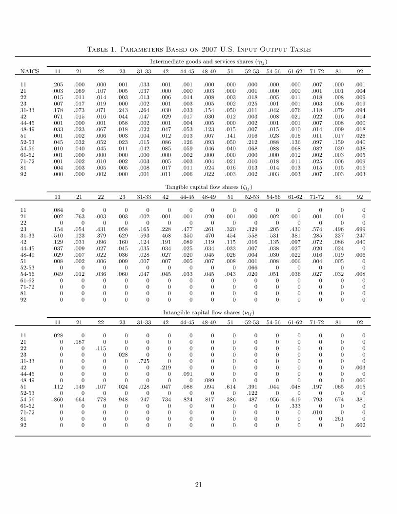
Table 1. Parameters Based on 2007 U.S. Input Output Table

Intermediate goods and services shares (γlj)

NAICS 11 21 22 23 31-33 42 44-45 48-49 51 52-53 54-56 61-62 71-72 81 92

11 .205 .000 .000 .001 .033 .001 .001 .000 .000 .000 .000 .000 .007 .000 .00121 .003 .069 .107 .005 .037 .000 .000 .003 .000 .001 .000 .000 .001 .001 .00422 .015 .011 .014 .003 .013 .006 .014 .008 .003 .018 .005 .011 .018 .008 .00923 .007 .017 .019 .000 .002 .001 .003 .005 .002 .025 .001 .001 .003 .006 .01931-33 .178 .073 .071 .243 .264 .030 .033 .154 .050 .011 .042 .076 .118 .079 .09442 .071 .015 .016 .044 .047 .029 .017 .030 .012 .003 .008 .021 .022 .016 .01444-45 .001 .000 .001 .058 .002 .001 .004 .005 .000 .002 .001 .001 .007 .008 .00048-49 .033 .023 .067 .018 .022 .047 .053 .123 .015 .007 .015 .010 .014 .009 .01851 .001 .002 .006 .003 .004 .012 .013 .007 .141 .016 .023 .016 .011 .017 .02652-53 .045 .032 .052 .023 .015 .086 .126 .093 .050 .212 .088 .136 .097 .159 .04054-56 .010 .040 .045 .011 .042 .085 .059 .046 .040 .068 .088 .068 .082 .039 .03861-62 .001 .000 .000 .000 .000 .000 .002 .000 .000 .000 .000 .012 .002 .003 .00571-72 .001 .002 .010 .002 .003 .005 .003 .004 .021 .010 .018 .011 .025 .006 .00981 .004 .003 .005 .005 .008 .017 .011 .024 .016 .013 .014 .013 .015 .015 .01592 .000 .000 .002 .000 .001 .011 .006 .022 .003 .002 .003 .003 .007 .003 .003

Tangible capital flow shares (ζlj)

11 21 22 23 31-33 42 44-45 48-49 51 52-53 54-56 61-62 71-72 81 92

11 .084 0 0 0 0 0 0 0 0 0 0 0 0 0 021 .002 .763 .003 .003 .002 .001 .001 .020 .001 .000 .002 .001 .001 .001 022 0 0 0 0 0 0 0 0 0 0 0 0 0 0 023 .154 .054 .431 .058 .165 .228 .477 .261 .320 .329 .205 .430 .574 .496 .69931-33 .510 .123 .379 .629 .593 .468 .350 .470 .454 .558 .531 .381 .285 .337 .24742 .129 .031 .096 .160 .124 .191 .089 .119 .115 .016 .135 .097 .072 .086 .04044-45 .037 .009 .027 .045 .035 .034 .025 .034 .033 .007 .038 .027 .020 .024 048-49 .029 .007 .022 .036 .028 .027 .020 .045 .026 .004 .030 .022 .016 .019 .00651 .008 .002 .006 .009 .007 .007 .005 .007 .008 .001 .008 .006 .004 .005 052-53 0 0 0 0 0 0 0 0 0 .066 0 0 0 0 054-56 .049 .012 .036 .060 .047 .045 .033 .045 .043 .020 .051 .036 .027 .032 .00861-62 0 0 0 0 0 0 0 0 0 0 0 0 0 0 071-72 0 0 0 0 0 0 0 0 0 0 0 0 0 0 081 0 0 0 0 0 0 0 0 0 0 0 0 0 0 092 0 0 0 0 0 0 0 0 0 0 0 0 0 0 0

Intangible capital flow shares (νlj)

11 21 22 23 31-33 42 44-45 48-49 51 52-53 54-56 61-62 71-72 81 92

11 .028 0 0 0 0 0 0 0 0 0 0 0 0 0 021 0 .187 0 0 0 0 0 0 0 0 0 0 0 0 022 0 0 .115 0 0 0 0 0 0 0 0 0 0 0 023 0 0 0 .028 0 0 0 0 0 0 0 0 0 0 031-33 0 0 0 0 .725 0 0 0 0 0 0 0 0 0 042 0 0 0 0 0 .219 0 0 0 0 0 0 0 0 .00344-45 0 0 0 0 0 0 .091 0 0 0 0 0 0 0 048-49 0 0 0 0 0 0 0 .089 0 0 0 0 0 0 .00051 .112 .149 .107 .024 .028 .047 .086 .094 .614 .391 .044 .048 .197 .065 .01552-53 0 0 0 0 0 0 0 0 0 .122 0 0 0 0 054-56 .860 .664 .778 .948 .247 .734 .824 .817 .386 .487 .956 .619 .793 .674 .38161-62 0 0 0 0 0 0 0 0 0 0 0 .333 0 0 071-72 0 0 0 0 0 0 0 0 0 0 0 0 .010 0 081 0 0 0 0 0 0 0 0 0 0 0 0 0 .261 092 0 0 0 0 0 0 0 0 0 0 0 0 0 0 .602

21

Table 1. Parameters Based on 2007 U.S. Input Output Table (Cont.)

Tangible capital shares (θj)

NAICS 11 21 22 23 31-33 42 44-45 48-49 51 52-53 54-56 61-62 71-72 81 92

.301 .558 .384 .167 .165 .127 .136 .132 .201 .408 .059 .076 .142 .130 .102

Intangible capital shares (φj)

11 21 22 23 31-33 42 44-45 48-49 51 52-53 54-56 61-62 71-72 81 92

.006 .011 .038 .082 .193 .149 .072 .039 .236 .040 .178 .033 .061 .056 .083

Consumption shares (ωj)

11 21 22 23 31-33 42 44-45 48-49 51 52-53 54-56 61-62 71-72 81 92

.005 .000 .021 .000 .118 .038 .089 .022 .033 .202 .018 .163 .068 .031 .193

22

Table 2. Correlations Between Latent Sectoral TFPs and U.S. Data, 1948:1–2014:4

Gross Output GDP MeasuredLatent TFPs, by Sector Aggregate Own sector Aggregate Per Hour TFP

Agriculture (11) .25 .84 .25 .02 .15

Mining (21) .15 .86 .00 -.29 -.20

Utilities (22) .01 .71 -.04 -.02 -.05

Construction (23) .72 .90 .67 .25 .54

Manufacturing (31-33) .82 .91 .57 -.15 .22

Chemical Manufacturing .60 .87 .50 .05 .33

Wholesale Trade (42) .15 .51 -.07 -.12 -.12

Retail Trade (44-45) .54 .87 .36 .11 .27

Transportation & Warehousing (48-49) .50 .78 .43 -.22 .09

Information (51) .08 .44 -.04 -.05 -.05

Broadcasting & Telecommunications .77 .85 .69 .03 .39

Finance, Insurance & Real Estate (52-53) .62 .93 .50 .11 .35

Professional & Business Services (54-56) .14 .44 .19 .08 .13

Advertising .15 .27 .05 .11 .11

Education, Health & Social Services (61-62) -.24 .68 -.27 .44 .16

Leisure and Hospitality (71-72) .46 .71 .43 -.03 .20

Other Services (81) .20 .60 .22 .14 .20

Note: The statistics are constructed for the model with an unrestricted variance-covariance matrix for theTFP shocks.

23

Table 3. Variance Decomposition and Predicted Correlations, 1948:1–2014:4

Model with Unrestricted Variance-Covariance Structure for TFP Shocks

Variance Decomposition Factor Analysis

TFP Labor Factor Common FactorObservable Shocks Wedge Loadings Contribution

Gross Outputs, by sector:

Agriculture (11) 99.86 0.14 -0.014 1.37

Mining (21) 100.00 0.00 0.051 4.37

Utilities (22) 99.92 0.08 0.015 0.33

Construction (23) 99.74 0.26 -0.005 1.12

Manufacturing (31-33) 99.93 0.07 0.026 15.92

Chemical Manufacturing 99.90 0.10 -0.004 0.83

Wholesale Trade (42) 99.72 0.28 0.029 61.85

Retail Trade (44-45) 99.44 0.56 0.016 38.57

Transportation & Warehousing (48-49) 99.80 0.20 0.010 10.31

Information (51) 99.73 0.27 0.013 2.73

Broadcasting & Telecommunications 99.51 0.49 -0.003 1.28

Finance, Insurance & Real Estate (52-53) 99.90 0.10 0.013 16.46

Professional & Business Services (54-56) 99.39 0.61 -0.036 43.53

Advertising 99.57 0.43 0.033 52.88

Education, Health & Social Services (61-62) 99.30 0.70 0.002 6.15

Leisure and Hospitality (71-72) 99.67 0.33 -0.000 0.01

Other Services (81) 99.37 0.63 0.004 1.78

Total Gross Output 99.79 0.21 – –

Total Hours 65.01 34.99 – –

24

Table 4. Variance Decomposition with Detail for TFP Shocks, 1948:1–2014:4

Model with Restricted Variance-Covariance Structure for TFP Shocks

TFP Shocks

Sector-specific

Own Other Common LaborObservable Total Industry Industry Shock Wedge

Gross Outputs, by sector:

Agriculture (11) 81.45 5.95 75.50 18.40 0.15

Mining (21) 99.08 97.26 1.82 0.92 0.00

Utilities (22) 84.56 11.36 73.20 15.35 0.09

Construction (23) 86.93 48.13 38.81 12.76 0.30

Manufacturing (31-33) 90.51 74.36 16.16 9.40 0.08

Chemical Manufacturing 87.20 66.31 20.89 12.70 0.10

Wholesale Trade (42) 82.31 59.11 23.19 17.34 0.36

Retail Trade (44-45) 53.16 3.92 49.24 46.36 0.48

Transportation & Warehousing (48-49) 67.60 3.19 64.41 31.95 0.45

Information (51) 68.01 1.93 66.09 31.72 0.27

Broadcasting & Telecommunications 69.64 2.92 66.72 29.90 0.47

Finance, Insurance & Real Estate (52-53) 76.47 1.15 75.32 23.43 0.10

Professional & Business Services (54-56) 80.05 71.18 8.87 19.34 0.61

Advertising 92.03 88.85 3.18 7.55 0.42

Education, Health & Social Services (61-62) 44.53 1.63 42.90 55.01 0.46

Leisure and Hospitality (71-72) 60.04 1.07 58.96 39.67 0.29

Other Services (81) 53.75 2.08 51.67 45.74 0.51

Total Gross Output 78.49 − − 21.27 0.25

Total hours 48.50 − − 10.28 41.22

25

Figure 1Input Output Table

Inte

rmed

iate

Purc

hases

Con

sum

ptio

n

Intan

gible

Inve

stmen

ts

Com

mod

ities

Industries

Com

mod

ity O

utpu

t

Gov

t. C

onsu

mpt

ion

Net

exp

orts

Industry Output

Final Uses

Tang

ible

Inve

stmen

ts

Compensation

Business taxes

Operating surplus

(J x J)(J x J) (J x J)

Val

ue A

dded

Compute GDP by summing: 1. Industry output less intermediates 2. Value added components, or 3. Final expenditures

26

Figure 2U.S. Gross Output and Two Measures of Aggregate TFP

A. 1980:1-1985:4

1980 1981 1982 1983 1984 1985 1986-.08

-.04

0

.04

.08

Gross outputMeasured TFPModel common TFP

B. 2008:1-2014:4

2008 2009 2010 2011 2012 2013 2014 2015-.08

-.04

0

.04

.08

Gross outputMeasured TFPModel common TFP

Note: The predicted series is based on the model with a restricted variance-covariance matrix for the TFPshocks.

27

Figure 3Total Gross Output, Actual and Model Forecast

A. 1980:1-1985:4

1980 1981 1982 1983 1984 1985 1986-.08

-.04

0

.04

.08

Gross outputModel forecast

B. 2008:1-2014:4

2008 2009 2010 2011 2012 2013 2014 2015-.08

-.04

0

.04

.08

Gross outputModel forecast

Note: The predicted series is based on the model with an unrestricted variance-covariance matrix for the TFPshocks. The estimates are nearly the same in the model with a restricted variance-covariance structure andare therefore not shown.

28

Figure 4Hours Per Capita, Actual and Model Forecast

A. 1980:1-1985:4

1980 1981 1982 1983 1984 1985 1986-.06

-.03

0

.03

.06

Per capita hoursModel forecast

B. 2008:1-2014:4

2008 2009 2010 2011 2012 2013 2014 2015-.06

-.03

0

.03

.06

Per capita hoursModel forecast

Note: The predicted series is based on the model with an unrestricted variance-covariance matrix for the TFPshocks. The estimates are nearly the same in the model with a restricted variance-covariance structure andare therefore not shown.

29