almost sure invariance principle for dynamical systems

Hiroshima Math. J.

34 (2004), 371–411

Almost sure invariance principle for dynamical systems with

stretched exponential mixing rates

Naoki Nagayama

(Received September 5, 2003)

Abstract. We prove the almost sure invariance principle for a class of abstract

dynamical systems including dynamical systems with stretched exponential mixing rates.

The result can be applied to chaotic billiards and hyperbolic attractors with Markov

sieves as well as expanding maps of the interval and Axiom A di¤eomorphisms.

1. Introduction

Let T be a measure preserving transformation on a probability space

ðM;B; mÞ and F an element of L2ðM;B; mÞ. We are interested in the limiting

behavior of the random process fSNgyN¼1 on ðM;B; mÞ defined by SN ¼PN�1i¼0 F � T i. Especially the central limit theorem, the weak invariance prin-

ciple, the almost sure invariance principle, and the law of the iterated logarithm

are our main concern. It is well known that the almost sure invariance

principle implies the other limit theorems above. Therefore we shall devote

ourselves to the almost sure invariance principle in the sequel. For the sake of

simplicity we say that the almost sure invariance principle holds for F (with

l A ð0; 1=2Þ) if the process fSNgyN¼1 satisfies the following property.

Without changing the distribution, we can redefine the random process

fSNgyN¼1 on a richer probability space together with a Brownian motion

fBðtÞgt A ½0;yÞ such that

SN � E½SN � ¼ Bðs2FNÞ þOðN 1

2�lÞ ðN ! yÞ m-a:s: ð1:1Þ

holds for some positive number l A ð0; 1=2Þ.Here s2

F denotes the limiting variance defined by s2F ¼ CF ð0Þþ

2Py

n¼1 CF ðnÞ, where CF ðnÞ are the autocorrelation coe‰cients of F given by

the formula

CF ðnÞ ¼ðM

F ðxÞFðT nxÞdmðxÞ � ðE½F �Þ2 n ¼ 0; 1; 2; . . . : ð1:2Þ

2000 Mathematics Subject Classification. Primary 60F15; Secondary 60F15, 37D45, 37D50

Key words and phrases. almost sure invariance principle, chaotic billiard, hyperbolic attractor

In [8, Theorem 7.1], Philipp and Stout give a su‰cient condition for the almost

sure invariance principle for mixing random processes in a quite general setup.

This theorem is known to be applicable to the process fSNgyN¼1 in the following

cases. (1) T is a uniformly expanding transformation on the unit interval ½0; 1�(L-Y map) and F is of bounded p-variation with some pf 1 and (2) T is an

Axiom A di¤eomorphism on a compact manifold and F is Holder continuous.

The reason why the Philipp-Stout theorem works well in these cases is that

these dynamical systems have nice measurable partitions such as the generating

partition for T in the case (1) and the Markov partition for T in the case (2)

(see [6] and [2]). More precisely, one can apply the Philipp-Stout theorem if

M is a separable metric space and there exists a finite or countable measurable

partition A having the following properties.

( i ) There exist positive constants C1 and k1 with 0 < k1 < 1 such that

diam 4N

i¼0

T�iA

!eC1k

N1 ð1:3Þ

holds for any nonnegative integer N, or T is invertible and T�1 is

also measurable and

diam 4N

i¼�N

T�iA

!eC1k

N1 ð1:4Þ

holds for any nonnegative integer N.

(ii) There exist positive constants C2 and k2 with 0 < k2 < 1 such that

b 4k

i¼0

T�iA; 4kþnþl

i¼kþn

T�iA

!eC2k

n2 ð1:5Þ

holds for any nonnegative integers k; l and n, where

bðA1;A2Þ ¼X

A1 AA1;A2 AA2

jmðA1 VA2Þ � mðA1ÞmðA2Þj ð1:6Þ

for finite or countable measurable partitions A1 and A2.

On the other hand many researchers have been interested in the stochastic

behavior of the dynamical systems such as the hyperbolic billiards and the

hyperbolic attractors. But in the case of the hyperbolic billiard it seems hard

to prove the almost sure invariance principle by the direct application of the

Philipp-Stout theorem since we do not have a measurable partition satisfying

the above conditions. It is remarkable that Chernov succeeded in proving the

weak invariance principle for the dynamical systems having stretched expo-

nential mixing rates in [4]. We recall that a dynamical system T on a metric

Naoki Nagayama372

space M is said to have stretched exponential mixing rates if it satisfies the

following.

There exists a constant y A ð0; 1� such that for any a A ð0; 1� there exists

a sequence fAðN;aÞgyN¼1 of finite or countable measurable partitions of M

satisfying;

( i ) there exist positive constants C1 and l1 with 0 < l1 < 1 such that

diamðAðN;aÞÞeC1lN ay

1 ð1:7Þ

holds for any positive integer N;

(ii) there exist positive constants C2 and l2 with 0 < l2 < 1 such that

bAðN; aÞ ðN; ½Na�ÞeC2lN ay

2 ð1:8Þ

holds for any positive integer N, where

bAðN; nÞ ¼ sup0ekeN�n

b 4k

i¼0

T�iA; 4N

i¼kþn

T�iA

!ð1:9Þ

for a finite or countable measurable partition A and nonnegative

integers N and n with neN.

The constants C1;C2; l1 and l2 in the above may depend on a

but not on N.

We note that the hyperbolic billiards and hyperbolic attractors are typical

examples which have stretched exponential mixing rates (see section 7 of [4],

c.f. [1], [3]).

In this paper, we aim to establish the almost sure invariance principle

for the dynamical systems with stretched exponential mixing rates inspired by

Chernov’s results in [4]. To this end, we first prove a slightly abstract result

for the dynamical system which has a special family of measurable partitions

(see Theorem 2.1). Afterward, it is shown that the dynamical systems with

stretched exponential mixing rates has such a family. As a consequence we

show the following theorem (see Remark just after Corollary 2.3).

Theorem 1.1. Assume that a dynamical system ðM;B; m;TÞ have stretched

exponential mixing rates. Let F be a Holder continuous function belonging to

L2þdðM;B; mÞ for some d with 0 < d < 2. Then the limiting variance s2F exists

and if it is positive, the almost sure invariance principle holds for F with any

positive number l < d8þ6d .

The organization of this paper is as follows. In Section 2, we first in-

troduce some definitions and notations. Next, we give the statement of the

main theorem (Theorem 2.1), which is more or less abstract. The almost sure

invariance principle for dynamical systems with stretched mixing rates will also

Almost sure invariance principle 373

be given as corollaries to the theorem. In Section 3, we mention about two

examples to which our results can be applied. Finally, Section 4 is devoted to

the proof of our results.

The author would like to express his gratitude to Professor Takehiko

Morita and Professor Hidekazu Ito for their helpful suggestion and advice.

2. Preliminaries and statement of results

Let T be a measure preserving transformation on a probability space

ðM;B; mÞ. We call the quartet ðM;B; m;TÞ a measure preserving dynamical

system. Throughout the paper all functions are assumed to be real valued.

First of all, we define autocorrelation coe‰cients of the stationary process

fF � T igyi¼0 by

CF ðnÞ ¼ðM

FðxÞF ðT nxÞdmðxÞ � ðE½F �Þ2 ðn ¼ 0; 1; 2; 3; . . .Þ: ð2:1Þ

We note that if

Xyn¼1

jCF ðnÞj < y ð2:2Þ

is satisfied, then we have

CF ð0Þ þ 2Xyn¼1

CF ðnÞ !

� V ½SN �N

�� ¼ 2

XNn¼1

n

NCF ðnÞ þ 2

Xyn¼Nþ1

CF ðnÞ��

��e 2

XNn¼1

n

NjCF ðnÞj þ 2

Xyn¼Nþ1

jCF ðnÞj

e 2X½ ffiffiffiNp

�

n¼1

½ffiffiffiffiffiN

p�

NjCF ðnÞj þ 2

Xyn¼½

ffiffiffiN

p�þ1

jCF ðnÞj

e2ffiffiffiffiffiN

pXyn¼1

jCF ðnÞj þ 2Xy

n¼½ffiffiffiN

p�þ1

jCF ðnÞj

! 0 ðN ! yÞ: ð2:3Þ

Therefore, we obtain

limN!y

V ½SN �N

¼ CF ð0Þ þ 2Xyn¼1

CF ðnÞ ¼ s2F : ð2:4Þ

Naoki Nagayama374

Next we introduce some definitions and notations. We say a finite or count-

able family of measurable sets A¼ fAigi A I (I ¼ N or I ¼ f1; 2; 3; . . . ; lg ðl A NÞ)a measurable partition of the probability space ðM;B; mÞ if mðAi VAjÞ ¼ 0 for

any i; j with i0 j and M ¼ 6i A I Ai up to m-null set. For a measurable

partition A ¼ fAigi A I and a nonnegative integer n we define a new measur-

able partition T�nA by T�nA ¼ fT�nAigi A I . For two measurable parti-

tions A ¼ fAigi A I and A 0 ¼ fA 0jgj A J we denote the new measurable partition

fAi VA 0jgi A I ; j A J by A4A 0. Besides, for finitely many measurable partitions

A1;A2; . . . ;AN we denote the measurable partition A14A24� � �4AN by

4N

k¼1

Ak.

For measurable partitions A ¼ fAigi A I and A 0 ¼ fA 0jgj A J we define a

measure of their independence bðA;A 0Þ by

bðA;A 0Þ ¼X

i A I ; j A J

jmðAi VA 0j Þ � mðAiÞmðA 0

j Þj: ð2:5Þ

For a measurable partition A and integers n;N with 0e neN we define

bAðN; nÞ ¼ sup0eleN�n

b 4l

k¼0

T�kA; 4N

k¼lþn

T�kA

!: ð2:6Þ

We denote by sðAÞ the s algebra generated by a family A of subsets of

M. We also denote by sðX1;X2; . . . ;XNÞ and sðX1;X2; . . .Þ, the s algebras

generated by random variables fXkgNk¼1 and fXkgyk¼1, respectively.

If the space M is endowed with a metric dM , the diameter of a measurable

partition A ¼ fAigi A I is defined by

diamðAÞ ¼ supi A I

supx;y AAi

dMðx; yÞ: ð2:7Þ

Moreover if the metric space M is separable and B is the topological Borel s

algebra of M, for F A L2ðM;B; mÞ and any positive number d we put

HF ðdÞ ¼ supA:measurable partition

diamðAÞed

kF � E½F j sðAÞ�k2: ð2:8Þ

In the above and also in what follows, we regard 1pas 0 when p ¼ y. Now

we are in a position to state our results.

Theorem 2.1. Let ðM;B; m;TÞ be a measure preserving dynamical system,

d be a positive constant, and r be a constant with 0e r < 1. Assume that a

function F A L2þdðM;B; mÞ satisfies


Xyn¼1

jCF ðnÞj < y ð2:9Þ

and

XNn¼1

nCF ðnÞ þXy

n¼Nþ1

NCF ðnÞ ¼ OðN rÞ ðN ! yÞ: ð2:10Þ

Furthermore we assume that there exist constants s; g with 0 < s < min d2þ2d ;

13

n o,

g > max2ð2þdÞð1�sÞd�ð2þ2dÞs ; 1�s

s

n oand a sequence of measurable partitions fAðNÞgN AN

satisfying the following properties.

( i )

bAðNÞ ðN; ½Ns�Þ ¼ OðN�gsÞ ðN ! yÞ: ð2:11Þ

(ii) There are constants p; t with 1e pey, t > 52 þ 1

pþ 1þ 1

p

� �gs and it

holds that

kF � E½F j sðAðNÞÞ�kp ¼ OðN�tÞ ðN ! yÞ: ð2:12Þ

Then the almost sure invariance principle holds for F provided sF 0 0.

Remark. It is easy to see from (2.4) that the weak invariance principle

and the law of iterated logarithm follow from the almost sure invariance

principle when the conditionsPy

n¼1 jCF ðnÞj < y and sF 0 0 are satisfied. On

the other hand the central limit theorem always follows from the weak invari-

ance principle. Consequently if the conditions of Theorem 2.1 are satisfied, all

the limit theorems that we mentioned in Introduction are valid.

From Theorem 2.1 and its proof we obtain the following corollaries.

Corollary 2.2. Let ðM;B; m;TÞ have stretched exponential mixing rates

and let F be a member of F A L2þdðM;B; mÞ for a positive number d. Assume

that there exists a number v > 24þ15dyd

such that

HF ðdÞ ¼ O1

jlog djv� �

ðd # 0Þ: ð2:13Þ

Then the almost sure invariance principle holds for F provided sF 0 0.

Corollary 2.3. Let ðM;B; m;TÞ have stretched exponential mixing rates

and let F be a member of F A L2þdðM;B; mÞ for a positive number d with

0 < de 2. Assume that for any positive number v the function F satisfies the

condition

HF ðdÞ ¼ O1

jlog djv� �

ðd # 0Þ:

Naoki Nagayama376

Then the almost sure invariance principle holds for F with any positive number

l < d8þ6d provided sF 0 0.

Remark. If the function F is Holder continuous, it satisfies the condition

HF ðdÞ ¼ O1

jlog djv� �

ðd # 0Þ

for any positive number v. Hence Theorem 1.1 immediately follows from

Corollary 2.3.

Remark. We must discuss the condition sF 0 0. Suppose that

Xyn¼1

njCF ðnÞj < y: ð2:14Þ

Then we see that sF ¼ 0 is equivalent to limN!y

V ½SN � < y by the expansion

V ½SN � ¼ s2FN � 2

XNn¼1

nCF ðnÞ � 2Xy

n¼Nþ1

NCF ðnÞ:

On the other hand, under the condition limn!y

CF ðnÞ ¼ 0, it is easy to see that

limN!y V ½SN � < y holds if and only if there exists a function G A L2ðM;B; mÞsuch that F ¼ G � G � T þ E½F � holds (see [7 Theorem 18.2.2]). Consequently

under the assumption (2.14) we can conclude that sF ¼ 0 if and only if there

exists a function G A L2ðM;B; mÞ such that F ¼ G � G � T þ E½F �. But it is

not easy to see whether there exists the function G such that F ¼ G � G � T þE½F � for a given function F . Therefore it is a troublesome problem to check

the condition sF 0 0 for a given function F . So it is remarkable that if F is

the first collision time of the two dimensional hyperbolic billiard with finite

horizon, then F satisfies sF 0 0 as well as the condition (2.13) (see [3, Section

7]). It provide us with a non trivial and interesting example to which our

result is applicable.

3. Examples

In this section we give two examples with Markov sieve. To such

dynamical systems not only Chernov’s results in [4] but also ours are appli-

cable.

(1) Two dimensional hyperbolic billiards.

Let Q be a compact closed domain on a plane or 2-torus. We assume

that the boundary qQ consists of finitely many smooth (of class C3) com-

ponents Gi ð1e ie dÞ each of whixh satisfies the following conditions.


(a) Gi is strictly convex as seen from the inside of Q.

(b) Gi is a rectilinear segment.

(c) Gi is a convex (as seen from the outside of Q) incomplete arc of a

circle whose complement to complete the circle do not intersect the

other components of qQ.

Now we put M0 ¼ fðq; vÞ A Q� S1 j q A qQn 61ei<jed

ðGi VGjÞ; hnðqÞ; vi > 0g,

where nðqÞ is the unit interior normal vector of qQ at the point q and h� ; �irepresents the ordinal inner product in the Euclidean space. We denote the

closure of M0 in Q� S1 by M, then we have MH qQ� S1. We define a map

T from M to itself by the following way.

Let ðq; vÞ be a point of M. We suppose that a point particle runs into

qQ at q with velocity v and next runs into qQ again at q 0 with velocity v 0

after the elastic reflection (reflection such that the angle of incidence equals

the angle of reflection) at q and motion of constant velocity in Q. Then

we define Tðq; vÞ ¼ ðq 0; v 0Þ. But when q is an end point of Gi, we define

Tðq; vÞ ¼ ðq; vÞ since we can not define Tðq; vÞ as above. In the case (b) or

(c), since we can not define T as above for the point ðq; vÞ of M such that

q A Gi and hnðqÞ; vi ¼ 0, we need some idea to define T well. We omit

details.

We denote the parameter representing length of qQ by r and the parameter

representing angle of v A S1 by j. Then r and j make natural coordinates of

qQ� S1 and we think qQ� S1 is a metric space by the coordinates. In what

follows we think M is a metric space as a subset of qQ� S1. Now we define

a probability measure m on ðM;BÞ (B is the topological Borel s algebra

of the metric space M) by dm ¼ cm cos j dr� dj, where cm is a normalizing

factor. Then it is known that ðM;B; m;TÞ is a measure preserving dynamical

system.

In [3] and [4], it is shown that a generic class of hyperbolic billiards admits

a family fRN;mg1em<N;N AN of family of measurable subsets of M satisfying

following conditions.

( i ) Each RN;m consists finitely many measurable subsets RðN;mÞ1 ; . . . ;

RðN;mÞl of M and when i0 j, it holds that R

ðN;mÞi VR

ðN;mÞj ¼ f.

( ii ) There are positive constants K1; a1 independent of N;m such that

0 < a1 < 1 and it holds that

max1eiel

supx;y ARðN ;mÞ

i

dðx; yÞeK1am1 ð3:1Þ

for any positive integers N;m with m < N, where d is the metric

of M.

(iii) There are positive constants K2; a2 independent of N;m such that

Naoki Nagayama378

0 < a2 < 1 and it holds that mðRðN;mÞ0 ÞeK2a

m2 for any positive

integers N;m with m < N, where RðN;mÞ0 ¼ Mn6

l

i¼1

RðN;mÞi .

(iv) There are positive constants K3; a3 independent of N;m such that

0 < a3 < 1 and it holds for any positive integer neN and

ði0; . . . ; inÞ A f1; . . . ; lgnþ1 that jDjeK3, where D is the real number

such that

mðT�nRðN;mÞin

jT�ðn�1ÞRðN;mÞin�1

V � � �VRðN;mÞi0

Þ

¼ mðT�1RðN;mÞin

jRðN;mÞin�1

Þð1þ DÞ: ð3:2Þ

( v ) There are positive constants K4; a4; g0; g1 independent of N;m such

that 0 < a4 < 1 and it holds that for any positive integer k with

kf ½g0m� that

X1eiel

Tj ASðiÞ

mðRðN;mÞj

Þ>1�K4Nam4

mðRðN;mÞi Þ > 1� K4Nam

4 ; ð3:3Þ

where SðiÞ ¼ f j A N j 1e je l; mðT�kRðN;mÞj jRðN;mÞ

i Þf g1mðRðN;mÞj Þg.

Note that such a family fRN;mg1em<N;N AN is called a Markov sieve. We

can show the dynamical system ðM;B; m;TÞ has stretched exponential mixing

rates by using Markov sieve (see [4]). Thus we can apply Corollary 2.2 and

Corollary 2.3 to this system.

(2) Two dimensional hyperbolic attractors.

Let M be a smooth two dimensional Riemannian manifold, U be an open

connected subset of M with compact closure and G be a closed subset of U .

We assume that the set Sþ ¼ G U qU consists of a finite number of compact

smooth curves. Let T : UnG ! U be a C2-di¤eomorphism from the open set

UnG onto its image TðUnGÞ. We assume that T is di¤erentiable on UnG up

to its boundary qðUnGÞ ¼ Sþ. Also we assume that T�1 is di¤erentiable on

TðUnGÞ up to its boundary qðTðUnGÞÞ.Denote Uþ ¼ fx A U jT nx A UnG for any nonnegative integer ng and

D ¼ 7y

n¼0

T nðUþÞ. The set D is invariant for both T and T�1. Its closure

L ¼ D is called the attractor for T .

We define the cone Cðz;P; aÞ for z A U , a line P through the origin in

the tangent space TzM and a positive number a by Cðz; a;PÞ ¼ fv A TzM jffðP; vÞe ag. An attractor L is called a generalized hyperbolic attractor if


for each z A UnG there exist two cone CuðzÞ ¼ Cðz; auðzÞ;PuðzÞÞ and CsðzÞ ¼Cðz; asðzÞ;PsðzÞÞ having the following three properties:

(1)

infz AUnG

infv1 ACuðzÞv2 AC sðzÞ

ffðv1; v2Þ > 0;

(2) DTðCuðzÞÞHCuðTzÞ for any z A UnG and DT�1ðCsðzÞÞHCsðT�1zÞfor any z A TðUnGÞ;

(3) there exist a positive constant C and a constant l with 0 < l < 1 such

that for any positive integer

(a) if z A Uþ and if v A CuðzÞ, then kDT nvkfCl�nkvk;(b) if z A T nðUþÞ and if v A CsðzÞ then kDT�nvkfCl�nkvk.

If we assume some generic conditions on the singularity set of a gener-

alized hyperbolic attractor L, then there exist subsets Li ði ¼ 0; 1; 2; . . .Þ of L

and Gibbs u-measures (the definition is found in [1]) mi ði ¼ 1; 2; 3; . . .Þ, whichare T-invariant probability measures on ðL;BÞ (B is the topological Borel field

of L), satisfying:

(1) L ¼ 6if 0

Li and Li VLl ¼ f when i0 j;

(2) for if 1 Li HD, TðLiÞ ¼ Li, miðLiÞ ¼ 1 and T jLiis ergodic with

respect to mi;

(3) for if 1 there exists a decomposition of Li to its subsets Li ¼ 6ri

j¼1

Li; j

such that Li; j VLi; j 0 ¼ f if j0 j 0, TðLi; jÞ ¼ Li; jþ1 if 1e je ri � 1,

TðLi; riÞ ¼ Li;1 and T ri jLi; 1has the Bernoulli property.

Now we choose i with 1e i and j with 1e je ri arbitrarily, and write

L� ¼ Li; j, T� ¼ T ri jL�and m� ¼

mi jB�miðL�Þ (B� is the topological Borel s algebra of

L�). We consider the measure preserving dynamical system ðL�;B�; m�;T�Þ.In [1] Markov sieves have been constructed for this system. Note that the

definition of Markov sieve for a generalized hyperbolic attractor is slightly

di¤erent from that for hyperbolic billiards in the above. One has to replace

the condition (v) in the above by the following one:

(v 0) there are positive constants g0; g1 independent of N;m such that for

every integer kf ½g0m� and any pair of integer i; j with 1e i; je l

one has

1

2

Xl

h¼1

jm�ðT�k� R

ðN;mÞh jRðN;mÞ

i Þ � m�ðT�k� R

ðN;mÞh jRðN;mÞ

j Þj < 1� g1:

ð3:4ÞWe can show the dynamical system ðL�;B�; m�;T�Þ has stretched expo-

nential mixing rates by using Markov sieve (see [4]). Thus we can apply

Corollary 2.2 and Corollary 2.3 to this system.

Naoki Nagayama380

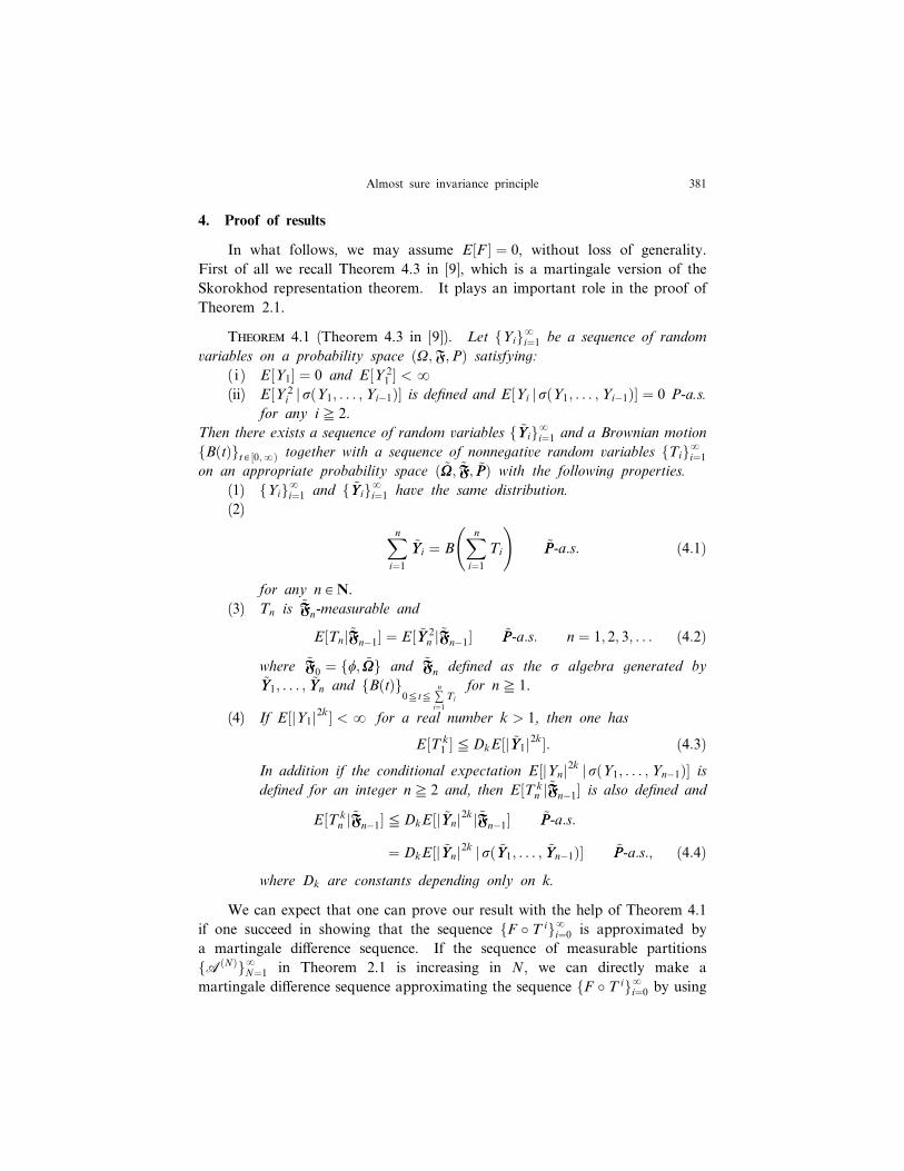
4. Proof of results

In what follows, we may assume E½F � ¼ 0, without loss of generality.

First of all we recall Theorem 4.3 in [9], which is a martingale version of the

Skorokhod representation theorem. It plays an important role in the proof of

Theorem 2.1.

Theorem 4.1 (Theorem 4.3 in [9]). Let fYigyi¼1 be a sequence of random

variables on a probability space ðW;F;PÞ satisfying:

( i ) E½Y1� ¼ 0 and E½Y 21 � < y

(ii) E½Y 2i j sðY1; . . . ;Yi�1Þ� is defined and E½Yi j sðY1; . . . ;Yi�1Þ� ¼ 0 P-a.s.

for any if 2.

Then there exists a sequence of random variables f ~YYigyi¼1 and a Brownian motion

fBðtÞgt A ½0;yÞ together with a sequence of nonnegative random variables fTigyi¼1

on an appropriate probability space ð ~WW; ~FF; ~PPÞ with the following properties.

(1) fYigyi¼1 and f ~YYigyi¼1 have the same distribution.

(2)

Xni¼1

~YYi ¼ BXni¼1

Ti

!~PP-a:s: ð4:1Þ

for any n A N.

(3) Tn is ~FFn-measurable and

E½Tnj~FFn�1� ¼ E½ ~YY 2n j~FFn�1� ~PP-a:s: n ¼ 1; 2; 3; . . . ð4:2Þ

where ~FF0 ¼ ff; ~WWg and ~FFn defined as the s algebra generated by~YY1; . . . ; ~YYn and fBðtÞg

0ete Tn

i¼1

Ti

for nf 1.

(4) If E½jY1j2k� < y for a real number k > 1, then one has

E½T k1 �eDkE½j ~YY1j2k�: ð4:3Þ

In addition if the conditional expectation E½jYnj2k j sðY1; . . . ;Yn�1Þ� isdefined for an integer nf 2 and, then E½T k

n j~FFn�1� is also defined and

E½T kn j~FFn�1�eDkE½j ~YYnj2kj~FFn�1� ~PP-a:s:

¼ DkE½j ~YYnj2k j sð ~YY1; . . . ; ~YYn�1Þ� ~PP-a:s:; ð4:4Þ

where Dk are constants depending only on k.

We can expect that one can prove our result with the help of Theorem 4.1

if one succeed in showing that the sequence fF � T igyi¼0 is approximated by

a martingale di¤erence sequence. If the sequence of measurable partitions

fAðNÞgyN¼1 in Theorem 2.1 is increasing in N, we can directly make a

martingale di¤erence sequence approximating the sequence fF � T igyi¼0 by using


fAðNÞgyN¼1. But unfortunately we can not expect such a situation in general.

Therefore we have to construct a new increasing sequence of measurable

partitions fUðNÞgyN¼1 which enjoy a nice properties with respect to the function

F . The next proposition plays a crucial role in the construction of the desired

partitions.

Proposition 4.2. Let l; g0 be positive numbers. Suppose that there exist

1e pey and t such that t > 52 þ 1

pþ 1þ 1

p

� �g0 þ l and

kF � E½F j sðAðNÞÞ�kp ¼ OðN�tÞ ðN ! yÞ ð4:5Þ

hold. Then, there exist constants 0e r0 < 1 and C0 such that the following

holds.

If we put

UðNÞk ¼ fx A M j r0 þ k � 2�½ð1=2þlÞ log2 N �

eF ðxÞ < r0 þ ðk þ 1Þ � 2�½ð1=2þlÞ log2 N �g;

then the family UðNÞ ¼ fU ðNÞk gk AZ of subset of M becomes a measurable

partition satisfying

bUðNÞ ðN; nÞe bAðNÞ ðN; nÞ þ C0N�g0 ð4:6Þ

for any pair of positive integers neN.

Proof. We have only to prove in the case when 1e p < y. We choose

a real number a with2þg0

tþ 1p�1

2�l< a <

p

pþ1 . This is possible because

t >5

2þ 1

pþ 1þ 1

p

� �g0 þ l , 2þ g0

tþ 1p� 1

2 � l<

p

pþ 1: ð4:7Þ

For N A N, 0e r < 1, and k A Z, we define the set UðNÞr;k by

UðNÞr;k ¼ fx A M j rþ k � 2�½ð1=2þlÞ log2 N � eF ðxÞ < rþ ðk þ 1Þ � 2�½ð1=2þlÞ log2 N �g:

ð4:8Þ

Writing AðNÞ as fAðNÞi gi A IN , for N A N and i A IN , we set

bN; i ¼0 if mðAðNÞ

i Þ ¼ 0;

1

mðAðNÞi

Þ

ÐA

ðNÞi

F dm if mðAðNÞi Þ > 0:

8<: ð4:9Þ

Next, for N A N, i A IN and 0e r < 1, we select the integer kðN; i; rÞ satisfying

rþ kðN; i; rÞ � 2�½ð1=2þlÞ log2 N �e bN; i < rþ ðkðN; i; rÞ þ 1Þ � 2�½ð1=2þlÞ log2 N �

ð4:10Þ

Take a positive integer N and fix it for a while. For r A ½0; 1Þ and i A IN ,

we set

Naoki Nagayama382

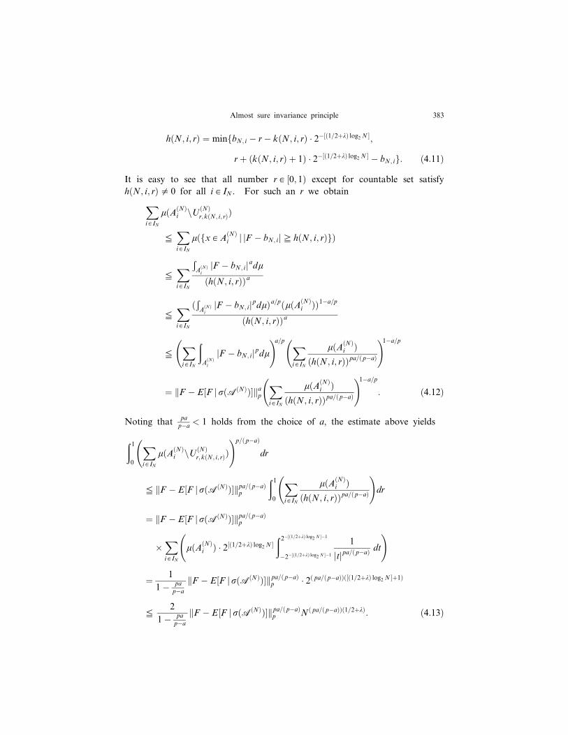
hðN; i; rÞ ¼ minfbN; i � r� kðN; i; rÞ � 2�½ð1=2þlÞ log2 N �;

rþ ðkðN; i; rÞ þ 1Þ � 2�½ð1=2þlÞ log2 N � � bN; ig: ð4:11Þ

It is easy to see that all number r A ½0; 1Þ except for countable set satisfy

hðN; i; rÞ0 0 for all i A IN . For such an r we obtainXi A IN

mðAðNÞi nU ðNÞ

r;kðN; i; rÞÞ

eXi A IN

mðfx A AðNÞi j jF � bN; ijf hðN; i; rÞgÞ

eXi A IN

ÐA

ðNÞi

jF � bN; ijadmðhðN; i; rÞÞa

eXi A IN

ðÐA

ðNÞi

jF � bN; ijpdmÞa=pðmðAðNÞi ÞÞ1�a=p

ðhðN; i; rÞÞa

eXi A IN

ðA

ðNÞi

jF � bN; ijpdm !a=p X

i A IN

mðAðNÞi Þ

ðhðN; i; rÞÞpa=ðp�aÞ

!1�a=p

¼ kF � E½F j sðAðNÞÞ�kapXi A IN

mðAðNÞi Þ

ðhðN; i; rÞÞpa=ðp�aÞ

!1�a=p

: ð4:12Þ

Noting thatpa

p�a< 1 holds from the choice of a, the estimate above yields

ð10

Xi A IN

mðAðNÞi nU ðNÞ

r;kðN; i; rÞÞ !p=ðp�aÞ

dr

e kF � E½F j sðAðNÞÞ�kpa=ðp�aÞp

ð10

Xi A IN

mðAðNÞi Þ

ðhðN; i; rÞÞpa=ð p�aÞ

!dr

¼ kF � E½F j sðAðNÞÞ�kpa=ðp�aÞp

�Xi A IN

mðAðNÞi Þ � 2½ð1=2þlÞ log2 N �

ð2�½ð1=2þlÞ log2 N ��1

�2�½ð1=2þlÞ log2 N ��1

1

jtjpa=ðp�aÞ dt

!

¼ 1

1� pa

p�a

kF � E½F j sðAðNÞÞ�kpa=ðp�aÞp � 2ð pa=ðp�aÞÞð½ð1=2þlÞ log2 N �þ1Þ

e2

1� pa

p�a

kF � E½F j sðAðNÞÞ�kpa=ð p�aÞp Nð pa=ðp�aÞÞð1=2þlÞ: ð4:13Þ


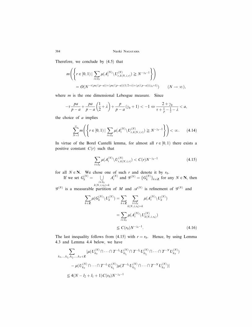
Therefore, we conclude by (4.5) that

m r A ½0; 1Þ jXi A IN

mðAðNÞi nU ðNÞ

r;kðN; i; rÞÞfN�g0�1

( ) !

¼ OðN�tðpa=ðp�aÞÞþðpa=ðp�aÞÞð1=2þlÞþð p=ðp�aÞÞðg0þ1ÞÞ ðN ! yÞ;

where m is the one dimensional Lebesgue measure. Since

�tpa

p� aþ pa

p� a

1

2þ l

� �þ p

p� aðg0 þ 1Þ < �1 , 2þ g0

tþ 1p� 1

2 � l< a;

the choice of a implies

XyN¼1

m r A ½0; 1Þ jXi A IN

mðAðNÞi nU ðNÞ

r;kðN; i; rÞÞfN�g0�1

( ) !< y: ð4:14Þ

In virtue of the Borel Cantelli lemma, for almost all r A ½0; 1Þ there exists a

positive constant CðrÞ such that

Xi A IN

mðAðNÞi nU ðNÞ

r;kðN; i; rÞÞ < CðrÞN�g0�1 ð4:15Þ

for all N A N. We chose one of such r and denote it by r0.

If we set GðNÞk ¼ 6

i A INkðN; i; r0Þ¼k

AðNÞi and GðNÞ ¼ fGðNÞ

k gk AZ for any N A N, then

GðNÞ is a measurable partition of M and AðNÞ is refinement of GðNÞ andXk AZ

mðGðNÞk nU ðNÞ

k Þ ¼Xk AZ

Xi A IN

kðN; i; r0Þ¼k

mðAðNÞi nU ðNÞ

k Þ

¼Xi A IN

mðAðNÞi nU ðNÞ

kðN; i; r0ÞÞ

eCðr0ÞN�g0�1: ð4:16Þ

The last inequality follows from (4.15) with r ¼ r0. Hence, by using Lemma

4.3 and Lemma 4.4 below, we haveXk0;...;kl1 ;kl2 ;...;kN AZ

jmðU ðNÞk0

V � � �VT�l1UðNÞkl1

VT�l2UðNÞkl2

V � � �VT�NUðNÞkN

Þ

� mðU ðNÞk0

V � � �VT�l1UðNÞkl1

ÞmðT�l2UðNÞkl2

V � � �VT�NUðNÞkN

Þj

e 4ðN � l2 þ l1 þ 1ÞCðr0ÞN�g0�1

Naoki Nagayama384

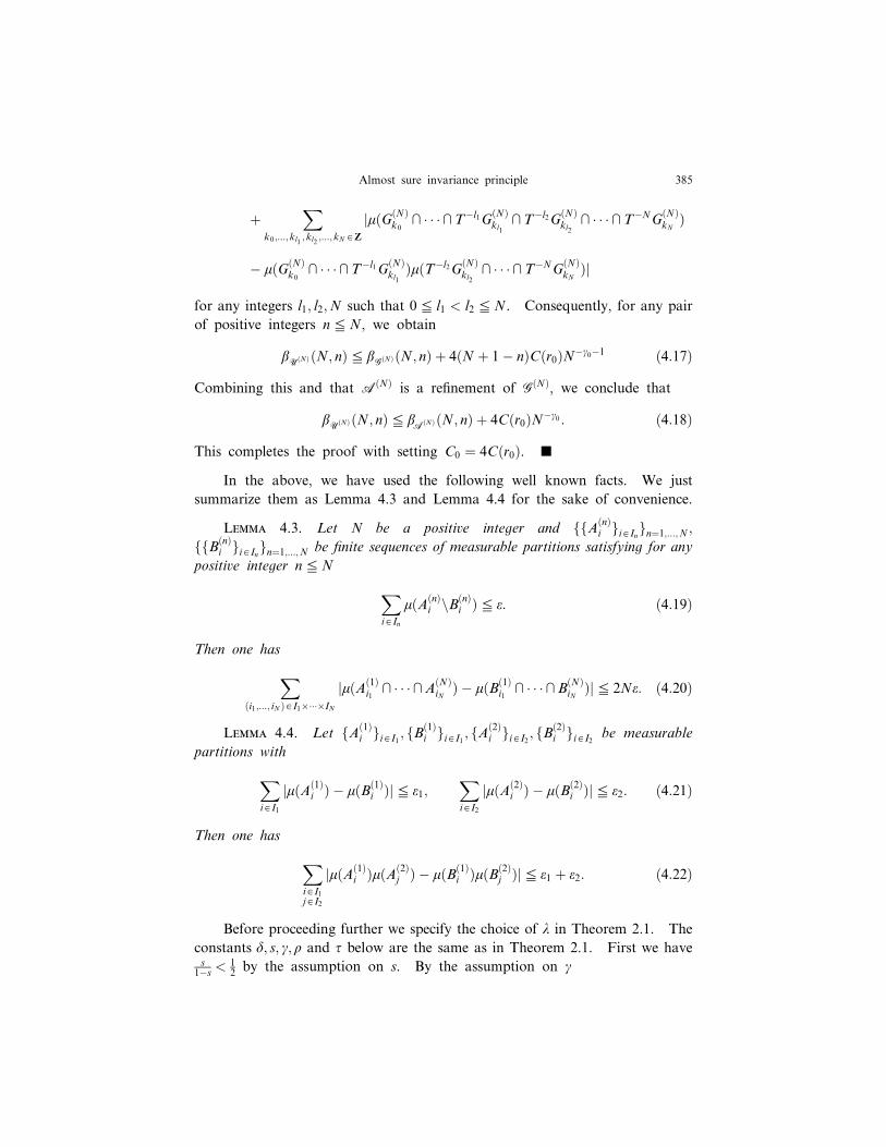
þX

k0;...;kl1 ;kl2 ;...;kN AZ

jmðGðNÞk0

V � � �VT�l1GðNÞkl1

VT�l2GðNÞkl2

V � � �VT�NGðNÞkN

Þ

� mðGðNÞk0

V � � �VT�l1GðNÞkl1

ÞmðT�l2GðNÞkl2

V � � �VT�NGðNÞkN

Þj

for any integers l1; l2;N such that 0e l1 < l2 eN. Consequently, for any pair

of positive integers neN, we obtain

bUðNÞ ðN; nÞe bGðNÞ ðN; nÞ þ 4ðN þ 1� nÞCðr0ÞN�g0�1 ð4:17Þ

Combining this and that AðNÞ is a refinement of GðNÞ, we conclude that

bUðNÞ ðN; nÞe bAðNÞ ðN; nÞ þ 4Cðr0ÞN�g0 : ð4:18Þ

This completes the proof with setting C0 ¼ 4Cðr0Þ. 9

In the above, we have used the following well known facts. We just

summarize them as Lemma 4.3 and Lemma 4.4 for the sake of convenience.

Lemma 4.3. Let N be a positive integer and ffAðnÞi gi A Ingn¼1;...;N ;

ffBðnÞi gi A Ingn¼1;...;N be finite sequences of measurable partitions satisfying for any

positive integer neN

Xi A In

mðAðnÞi nBðnÞ

i Þe e: ð4:19Þ

Then one has

Xði1;...; iN Þ A I1��IN

jmðAð1Þi1

V � � �VAðNÞiN

Þ � mðBð1Þi1

V � � �VBðNÞiN

Þje 2Ne: ð4:20Þ

Lemma 4.4. Let fAð1Þi gi A I1 ; fB

ð1Þi gi A I1 ; fA

ð2Þi gi A I2 ; fB

ð2Þi gi A I2 be measurable

partitions with

Xi A I1

jmðAð1Þi Þ � mðBð1Þ

i Þje e1;Xi A I2

jmðAð2Þi Þ � mðBð2Þ

i Þje e2: ð4:21Þ

Then one has

Xi A I1j A I2

jmðAð1Þi ÞmðAð2Þ

j Þ � mðBð1Þi ÞmðBð2Þ

j Þje e1 þ e2: ð4:22Þ

Before proceeding further we specify the choice of l in Theorem 2.1. The

constants d; s; g; r and t below are the same as in Theorem 2.1. First we haves

1�s< 1

2 by the assumption on s. By the assumption on g


d

2þ d� 2

g>

d

2þ d� d� ð2þ 2dÞsð2þ dÞð1� sÞ ¼

s

1� sð4:23Þ

holds. Next, we choose a real number a so that

s

1� s< a < min

1

2;

d

2þ d� 2

g

� �: ð4:24Þ

We notice that the number a chosen above satisfies sð1þ aÞ < a.

By g > 1�ss

and s1�s

< a < d2þd

� 2g< d

2þd, we obtain

sgd

4ð2þ dÞ �a

4ð1þ aÞ >ð1� sÞd4ð2þ dÞ �

a

4ð1þ aÞ >d� að2þ dÞ

4ð1þ aÞð2þ dÞ > 0: ð4:25Þ

Therefore, by the choice of a and the assumptions on r and t, we can choose

positive constants l; l 0 so that

l < l 0 < min

8<:

d� ð2þ dÞ aþ 2g

� �2ð1þ aÞð2þ dÞ ;

1� 2a

4ð1þ aÞ ;ð1� sÞa� s

2ð1þ aÞ ;ð1� rÞa2ð1þ aÞ ;

sgd

4ð2þ dÞ �a

4ð1þ aÞ ; t�5

2� 1

p� 1þ 1

p

� �gs

9=;: ð4:26Þ

We will prove Theorem 2.1 with l chosen above.

From now on, we can employ the methods similar to those that used in

the proof of Theorem 7.1 of [8].

We define two sequences fLjgyj¼0 and fMjgyj¼1 by

L0 ¼ 0; Lj ¼Xj

i¼1

½ia� þXj

i¼2

½i sð1þaÞ� ð j ¼ 1; 2; . . .Þ

and

M1 ¼ 0; Mj ¼Xj�1

i¼1

½ia� þXj

i¼2

½i sð1þaÞ� ð j ¼ 2; 3; . . .Þ

and we also define two sequences of random variables fyjgyj¼1 and fzjgyj¼2 by

yj ¼XLj�1

i¼Mj

F � T i ð j ¼ 1; 2; . . .Þ

zj ¼XMj�1

i¼Lj�1

F � T i ð j ¼ 2; 3; . . .Þ:

Naoki Nagayama386

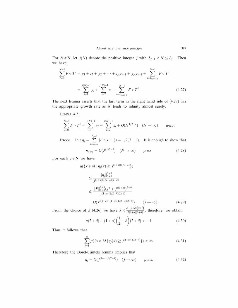
For N A N, let jðNÞ denote the positive integer j with Lj�1 < NeLj. Then

we have

XN�1

i¼0

F � T i ¼ y1 þ z2 þ y2 þ � � � þ zjðNÞ�1 þ yjðNÞ�1 þXN�1

i¼LjðNÞ�1

F � T i

¼XjðNÞ�1

i¼1

yi þXjðNÞ�1

i¼2

zi þXN�1

i¼LjðNÞ�1

F � T i: ð4:27Þ

The next lemma asserts that the last term in the right hand side of (4.27) has

the appropriate growth rate as N tends to infinity almost surely.

Lemma 4.5.

XN�1

i¼0

F � T i ¼XjðNÞ�1

i¼1

yi þXjðNÞ�1

i¼2

zi þOðN 1=2�lÞ ðN ! yÞ m-a:s:

Proof. Put hj ¼PLj�1

i¼Lj�1

jF � T ij ð j ¼ 1; 2; 3; . . .Þ. It is enough to show that

hjðNÞ ¼ OðN 1=2�lÞ ðN ! yÞ m-a:s: ð4:28Þ

For each j A N we have

mðfx A M j hjðxÞf jð1þaÞð1=2�lÞgÞ

ekhjk

2þd2þd

jð1þaÞð1=2�lÞð2þdÞ

ekFk2þd

2þdð j a þ j sð1þaÞÞ2þd

jð1þaÞð1=2�lÞð2þdÞ

¼ Oð j að2þdÞ�ð1þaÞð1=2�lÞð2þdÞÞ ð j ! yÞ: ð4:29Þ

From the choice of l (4.26) we have l <d�ð2þdÞ aþ2

gð Þ2ð1þaÞð2þdÞ , therefore, we obtain

að2þ dÞ � ð1þ aÞ 1

2� l

� �ð2þ dÞ < �1: ð4:30Þ

Thus it follows that

Xyj¼1

mðfx A M j hjðxÞf jð1þaÞð1=2�lÞgÞ < y: ð4:31Þ

Therefore the Borel-Cantelli lemma implies that

hj ¼ Oð jð1þaÞð1=2�lÞÞ ð j ! yÞ m-a:s: ð4:32Þ


On the other hand we have

jðNÞ ¼ OðN 1=ð1þaÞÞ ðN ! yÞ ð4:33Þ

by definition of jðNÞ. It is not hard to see that (4.28) follows from (4.32) and

(4.33). 9

Next we investigate the asymptotic behavior of the second term in the

right hand side of (4.27) as N tends to infinity.

Lemma 4.6.

XjðNÞ�1

i¼2

zi ¼ OðN 1=2�lÞ ðN ! yÞ m-a:s: ð4:34Þ

In order to prove the lemma we employ the Gaal-Koksma strong law of

large numbers in [8, Theorem A.1 of Appendix 1] as Lemma 4.7.

Lemma 4.7. Let fXkgyk¼1 be a sequence of random variables on a prob-

ability space ðW;F;PÞ whose expectations are 0. Suppose that there exist

positive constants s and C such that

EXnþm

k¼nþ1

Xk

!224

35eCððnþmÞs � nsÞ ð4:35Þ

for all nonnegative integer n and all positive integer m. Then

XNk¼1

Xk ¼ OðN s=2ðlog NÞ2þeÞ ðN ! yÞ P-a:s: ð4:36Þ

holds with any positive number e.

Proof of Lemma 4.6. If n and m are natural numbers, we have

ðM

Xnþm

j¼nþ1

zj

!2dme

Xnþm

j¼nþ1

XMj�1

k¼Lj�1

CF ð0Þ þ 2Xyn¼1

jCF ðnÞj !

¼ CF ð0Þ þ 2Xyn¼1

jCF ðnÞj ! Xnþm

j¼nþ1

½ j sð1þaÞ�

e c0ððnþmÞsð1þaÞþ1 � nsð1þaÞþ1Þ;

where c0 is a positive constant independent of n and m. Hence we can apply

Lemma 4.7. Note that 12 � l

ð1þ aÞ > sð1þaÞþ12 is valid since l <

ð1�sÞa�s

2ð1þaÞ holds

by (4.26). Thus we conclude that

Naoki Nagayama388

Xj

i¼1

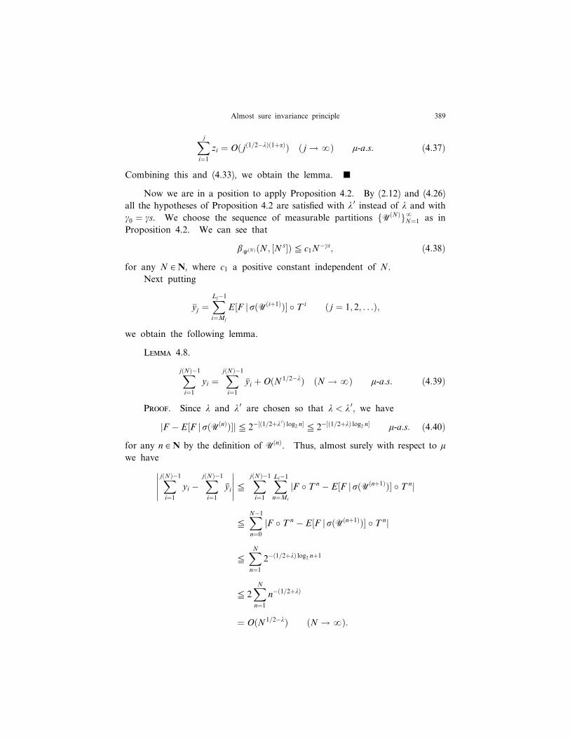
zi ¼ Oð jð1=2�lÞð1þaÞÞ ð j ! yÞ m-a:s: ð4:37Þ

Combining this and (4.33), we obtain the lemma. 9

Now we are in a position to apply Proposition 4.2. By (2.12) and (4.26)

all the hypotheses of Proposition 4.2 are satisfied with l 0 instead of l and with

g0 ¼ gs. We choose the sequence of measurable partitions fUðNÞgyN¼1 as in

Proposition 4.2. We can see that

bUðNÞ ðN; ½Ns�Þe c1N�gs; ð4:38Þ

for any N A N, where c1 a positive constant independent of N.

Next putting

yj ¼XLj�1

i¼Mj

E½F j sðUðiþ1ÞÞ� � T i ð j ¼ 1; 2; . . .Þ;

we obtain the following lemma.

Lemma 4.8.

XjðNÞ�1

i¼1

yi ¼XjðNÞ�1

i¼1

yi þOðN 1=2�lÞ ðN ! yÞ m-a:s: ð4:39Þ

Proof. Since l and l 0 are chosen so that l < l 0, we have

jF � E½F j sðUðnÞÞ�je 2�½ð1=2þl 0Þ log2 n� e 2�½ð1=2þlÞ log2 n� m-a:s: ð4:40Þ

for any n A N by the definition of UðnÞ. Thus, almost surely with respect to m

we have

XjðNÞ�1

i¼1

yi �XjðNÞ�1

i¼1

yi

��e

XjðNÞ�1

i¼1

XLi�1

n¼Mi

jF � T n � E½F j sðUðnþ1ÞÞ� � T nj

eXN�1

n¼0

jF � T n � E½F j sðUðnþ1ÞÞ� � T nj

eXNn¼1

2�ð1=2þlÞ log2 nþ1

e 2XNn¼1

n�ð1=2þlÞ

¼ OðN 1=2�lÞ ðN ! yÞ:


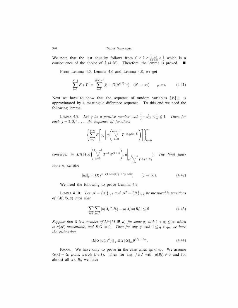
We note that the last equality follows from 0 < l < 1�2a4ð1þaÞ <

12 which is a

consequence of the choice of l (4.26). Therefore, the lemma is proved. 9

From Lemma 4.5, Lemma 4.6 and Lemma 4.8, we get

XN�1

i¼0

F � T i ¼XjðNÞ�1

i¼1

yi þOðN 1=2�lÞ ðN ! yÞ m-a:s: ð4:41Þ

Next we have to show that the sequence of random variables fyigyi¼1 is

approximated by a martingale di¤erence sequence. To this end we need the

following lemma.

Lemma 4.9. Let q be a positive number with 1gþ 1

2þd< 1

qe 1. Then, for

each j ¼ 2; 3; 4; . . . ; the sequence of functions

Xjþm

i¼j

E yi

�� s 4Lj�1�1

k¼0

T�kUðkþ1Þ

!" #( )ym¼0

converges in LqðM; s 4Lj�1�1

k¼0

T�kUðkþ1Þ

!; m

��sð 4

Lj�1�1

k¼0

T�kUðkþ1ÞÞ

Þ. The limit func-

tions uj satisfies

kujkq ¼ Oð j a�sð1þaÞgð1=q�1=ð2þdÞÞÞ ð j ! yÞ: ð4:42Þ

We need the following to prove Lemma 4.9.

Lemma 4.10. Let A ¼ fAigi A I and A 0 ¼ fBjgj A J be measurable partitions

of ðM;B; mÞ such that

Xi A I

Xj A J

jmðAi VBjÞ � mðAiÞmðBjÞje b: ð4:43Þ

Suppose that G is a member of Lq0ðM;B; mÞ for some q0 with 1 < q0 ey which

is sðAÞ-measurable, and E½G � ¼ 0. Then for any q with 1e q < q0, we have

the estimation

kE½G j sðA 0Þ�kq e 2kGkq0b1=q�1=q0 : ð4:44Þ

Proof. We have only to prove in the case when q0 < y. We assume

GðxÞ ¼ Gi m-a:s: x A Ai ði A IÞ. Then for any j A J with mðBjÞ0 0 and for

almost all x A Bj, we have

Naoki Nagayama390

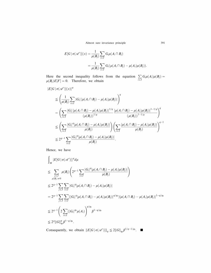
E½G j sðA 0Þ�ðxÞ ¼ 1

mðBjÞXi A I

GimðAi VBjÞ

¼ 1

mðBjÞXi A I

GiðmðAi VBjÞ � mðAiÞmðBjÞÞ:

Here the second inequality follows from the equationPi A I

GimðAiÞmðBjÞ ¼mðBjÞE½F � ¼ 0. Therefore, we obtain

jE½G j sðA 0Þ�ðxÞjq

e1

mðBjÞXi A I

jGij jmðAi VBjÞ � mðAiÞmðBjÞj !q

¼Xi A I

jGij jmðAi VBjÞ � mðAiÞmðBjÞj1=q

ðmðBjÞÞ1=qjmðAi VBjÞ � mðAiÞmðBjÞj1�1=q

ðmðBjÞÞ1�1=q

!q

eXi A I

jGijqjmðAi VBjÞ � mðAiÞmðBjÞjmðBjÞ

! Xi A I

jmðAi VBjÞ � mðAiÞmðBjÞjmðBjÞ

!q�1

e 2q�1Xi A I


:

Hence, we haveðM

jE½G j sðA 0Þ�jqdm

eXj A J

mðBjÞ00

mðBjÞ 2q�1Xi A I


!

e 2q�1Xj A J

Xi A I

jGijqjmðAi VBjÞ � mðAiÞmðBjÞj

¼ 2q�1Xj A J

Xi A I

ðjGijqjmðAi VBjÞ � mðAiÞmðBjÞjq=q0ÞjmðAi VBjÞ � mðAiÞmðBjÞj1�q=q0

e 2q�1 2Xi A I

ðjGijq0mðAiÞ !q=q0

b1�q=q0

e 2qkGkqq0b1�q=q0 :

Consequently, we obtain kE½G j sðA 0Þ�kq e 2kGkq0b1=q�1=q0 . 9


Proof of Lemma 4.9. First, we estimate E yj

�� s 4Lj�1�1

k¼0

T�kUðkþ1Þ

!" #��q

for any natural number jf 2. There exists a natural number Nj such that

½Nsj � ¼ Mj � ðLj�1 � 1Þ ¼ ½ j sð1þaÞ� þ 1. It can be checked easily by the defi-

nition of Lj that

Lj e j1þa ð j ¼ j0; j0 þ 1; j0 þ 2; . . .Þ ð4:45Þ

for j0 large enough. Therefore Lj < Nj holds for j0 e j by the definition of

Nj. Thus if j0 e j, we have

b 4Lj�1�1

k¼0

T�kUðkþ1Þ; 4Lj�1

k¼Mj

T�kUðkþ1Þ

!

e b 4Lj�1�1

k¼0

T�kUðNjÞ; 4Lj�1

k¼Mj

T�kUðNjÞ

!

e bUðNj Þ ðNj;Mj � ðLj�1 � 1ÞÞ

¼ bUðNj Þ ðNj; ½Ns

j �Þ

e c1N�gsj

e c1ð½ j sð1þaÞ� þ 1Þ�g

e c1 j�gsð1þaÞ

by using the inequality (4.38) and the choice of Nj. Here the first inequality

follows from the fact that UðNjÞ is a refinement of UðkÞ for any k < Lj by

Lj < Nj. Noting that yj is s 4Lj�1

k¼Mj

T�kUðkþ1Þ

!-measurable, we conclude from

Lemma 4.10 and the above estimation that

E yj

�� s 4Lj�1�1

k¼0

T�kUðkþ1Þ

!" #��q

e 2kyjk2þd � c1=q�1=ð2þdÞ1 j�gsð1þaÞð1=q�1=ð2þdÞÞ;

when j0 e j. Thus we can pick a positive constant c2 so that

E yj

�� s 4Lj�1�1

k¼0

T�kUðkþ1Þ

!" #��q

e c2 ja�gsð1þaÞð1=q�1=ð2þdÞÞ ð4:46Þ

holds for any jf 2.

Naoki Nagayama392

Next, we estimate E yj

�� s 4Ll�1

k¼0

T�kUðkþ1Þ

!" #��q

for any jf 3 and any

l with 1e le j � 2. There exists a natural number Nj; l such that ½Nsj; l � ¼

Mj � ðLl � 1Þ. Then it is obvious that Lj < Nj < Nj; l if jf j0. Thus if

jf j0, we have

b 4Ll�1

k¼0

T�kUðkþ1Þ; 4Lj�1

k¼Mj

T�kUðkþ1Þ

!

e b 4Ll�1

k¼0

T�kUðNj; lÞ; 4Lj�1

k¼Mj

T�kUðNj; lÞ

!

e bU

ðNj; l Þ ðNj ;Mj � ðLl � 1ÞÞ

¼ bU

ðNj; l Þ ðNj; l ; ½Nsj; l �Þ

e c1N�gsj; l

e c1ðMj þ 1� LlÞ�g ð4:47Þ

by using the inequality (4.38) and the choice of Nj. Here the first inequality

follows from the fact that UðNj; lÞ is a refinement of UðkÞ for any k < Lj by

Lj < Nj; l . Noting that yj is s 4Lj�1

k¼Mj

T�kUðkþ1Þ

!-measurable, we conclude

from Lemma 4.10 and the estimation above that

E yj

�� s 4Ll�1

k¼0

T�kUðkþ1Þ

!" #��q

e 2kyjk2þdðc1ðMj þ 1� LlÞ�gÞ1=q�1=ð2þdÞ: ð4:48Þ

Thus, by the definition of Mj and Ll , we can take a positive constant c3 so

that

E yj

�� s 4Ll�1

k¼0

T�kUðkþ1Þ

!" #��q

e c3 ja�agð1=q�1=ð2þdÞÞð j � 1� lÞ�gð1=q�1=ð2þdÞÞ

ð4:49Þ

holds for any jf 3 and any l with 1e le j � 2. By (4.46) and (4.49), we

obtain


Xyi¼j

E yi

�� s 4Lj�1�1

k¼0

T�kUðkþ1Þ

!" #��q

e c2 ja�gsð1þaÞð1=q�1=ð2þdÞÞ þ

Xym¼1

c3ð j þmÞa�agð1=q�1=ð2þdÞÞm�gð1=q�1=ð2þdÞÞ

e c2 ja�gsð1þaÞð1=q�1=ð2þdÞÞ þ c3

Xym¼1

j a�agð1=q�1=ð2þdÞÞm�gð1=q�1=ð2þdÞÞ

e c2 þ c3Xym¼1

m�gð1=q�1=ð2þdÞÞ

!j a�gsð1þaÞð1=q�1=ð2þdÞÞ:

In the above, the second inequality follows from a� ag 1q� 1

2þd

� �< 0 since

1gþ 1

2þd< 1

qand the third inequality follows from sð1þ aÞ < a (see (4.24)). In

addition we notice that

Xym¼1

m�gð1=q�1=ð2þdÞÞ < y

holds since 1gþ 1

2þd< 1

q. We have thus proved the lemma. 9

We note that 1gþ 1

2þd< 1

2 by the assumption on g. Let uj ð j ¼ 2; 3; 4; . . .Þbe as defined in Lemma 4.9 and u1 ¼ 0. If we define a sequence of functions

fYjgyj¼1 by

Yj ¼ yj � uj þ ujþ1;

then it is obvious by definition that fYjgyj¼1 is a martingale di¤erence sequence.

The following lemma gives the desired fact that fyigyi¼1 is approximated by a

martingale di¤erence sequence.

Lemma 4.11.

XjðNÞ�1

i¼1

yi ¼XjðNÞ�1

i¼1

Yi þOðN 1=2�lÞ ðN ! yÞ m-a:s: ð4:50Þ

Proof. First, we notice that

Xj

i¼1

Yi �Xj

i¼1

yi ¼Xj

i¼1

ðuiþ1 � uiÞ ¼ ujþ1 � u1 ¼ ujþ1 ð4:51Þ

holds for any natural number j. By g > 1�ss

and s1�s

< a, we have

Naoki Nagayama394

1

2þ s� 1

1þ aaþ 1

gþ 1

2þ d

� �>

d� að2þ dÞ2ð2þ dÞð1þ aÞ : ð4:52Þ

Combining this estimation with the inequality (4.26) we obtain l < 12 þ s�

11þa

aþ 1gþ 1

2þd

� �. Thus, noting that 1

gþ 1

2þd< 1

2 , we can choose qf 1 so that1gþ 1

2þd< 1

q< 1

2 � lþ s

ð1þ aÞ � a holds.

By (4.42) we obtain

mðfx A M j jujðxÞjf jð1=2�lÞð1þaÞgÞ

¼ Oð jða�sð1þaÞgð1=q�1=ð2þdÞÞÞq�ð1=2�lÞð1þaÞqÞ ð j ! yÞ: ð4:53Þ

The exponent in the right hand side is less than �1. Indeed,

a� sð1þ aÞg 1

q� 1

2þ d

� �� q� 1

2� l

� �ð1þ aÞq

< ða� sð1þ aÞÞq� 1

2� l

� �ð1þ aÞq

< �1

is valid since 1gþ 1

2þd< 1

qand 1

q< 1

2 � lþ s

ð1þ aÞ � a hold. Therefore, we

obtain

Xyj¼1

mðfx A M j jujðxÞjf jð1=2�lÞð1þaÞgÞ < y: ð4:54Þ

Hence by the Borel-Cantelli lemma we conclude that

uj ¼ Oð jð1=2�lÞð1þaÞÞ ð j ! yÞ m-a:s: ð4:55Þ

This with (4.33) and (4.51) completes the proof. 9

From Lemma 4.11 and the equality (4.41) we get

XN�1

k¼0

F � T k ¼XjðNÞ�1

i¼1

Yi þOðN 1=2�lÞ ðN ! yÞ m-a:s: ð4:56Þ

On the other hand we can apply Theorem 4.1 to fYjgyj¼1 since fYjgyj¼1 is a

martingale di¤erence sequence. In what follows, ð ~WW; ~FF; ~PPÞ; f ~YYigyi¼1; fTigyi¼1 and

fBðtÞgt A ½0;yÞ are as in Theorem 4.1. It remains to show that

BXjðNÞ�1

i¼1

Ti

!¼ Bðs2

FNÞ þOðN 1=2�lÞ ðN ! yÞ ~PP-a:s: ð4:57Þ

To this end we prove the following.


Lemma 4.12.

EXjðNÞ�1

i¼1

y2i

" #¼ s2

FN þOðN 1�2l 0Þ ðN ! yÞ:

Proof. For any positive integer N we have

EXjðNÞ�1

i¼1

y2i

" #¼XjðNÞ�1

i¼1

½ia�CF ð0Þ þ 2X½i a��1

n¼1

ð½ia� � nÞCF ðnÞ !

¼ Ns2F � s2

F

XjðNÞ�1

i¼2

½i sð1þaÞ� � s2F ðN � LjðNÞ�1Þ

� 2XjðNÞ�1

i¼1

X½i a�n¼1

nCF ðnÞ þ ½ia�Xy

n¼½i a�þ1

CF ðnÞ

0@

1A: ð4:58Þ

By l 0 <a�sð1þaÞ2ð1þaÞ we obtain

sð1þ aÞ þ 1 < ð1þ aÞð1� 2l 0Þ ð4:59Þ

This implies

XjðNÞ�1

i¼2

½i sð1þaÞ�eð jðNÞ

0

tsð1þaÞ dt ¼ Oð jðNÞð1þaÞð1�2l 0ÞÞ ðN ! yÞ: ð4:60Þ

Since a < 1 < sð1þ aÞ þ 1 < ð1þ aÞð1� 2l 0Þ holds from (4.59), we obtain

N � LjðNÞ�1 e ½ jðNÞa� þ ½ jðNÞsð1þaÞ� ¼ Oð jðNÞð1þaÞð1�2l 0ÞÞ ðN ! yÞð4:61Þ

It follows form the assumption (2.10) that

2XjðNÞ�1

i¼1

X½i a��1

n¼1

nCF ðnÞ þ ½ia�Xyn¼½i a�

CF ðnÞ

0@

1A

e 2c4

ð jðNÞ

0

tar dt

¼ Oð jðNÞarþ1Þ ðN ! yÞ

¼ Oð jðNÞð1þaÞð1�2l 0ÞÞ ðN ! yÞ; ð4:62Þ

Naoki Nagayama396

where c4 is a constant independent of N. Here we used the assumption that

l 0 <að1�rÞ2ð1þaÞ . Thus, from (4.58), (4.60), (4.61), (4.62) and (4.33) we conclude

that

EXjðNÞ�1

i¼1

y2i

" #¼ s2

FN þOðN 1�2l 0Þ ðN ! yÞ: ð4:63Þ

Next, by the definitions of yi and UðkÞ we have

EXjðNÞ�1

i¼1

y2i

" #� E

XjðNÞ�1

i¼1

y2i

" #��

e 2XjðNÞ�1

i¼1

kyik1XLi�1

k¼Mi

kF � E½F j sðUðkþ1ÞÞ�ky

þXjðNÞ�1

i¼1

XLi�1

k¼Mi

kF � E½F j sðUðkþ1ÞÞ�ky

!2

e 2XjðNÞ�1

i¼1

½ia�kFk1 � ½ia�2�½ð1=2þl 0Þ log2ðMiþ1Þ� þXjðNÞ�1

i¼1

½ia�22�2½ð1=2þl 0Þ log2ðMiþ1Þ�

¼ Oð jðNÞ2a�ð1þaÞð1=2þl 0ÞÞ ðN ! yÞ:

Since l 0 < 1�2a4ð1þaÞ <

1�a2ð1þaÞ holds from (4.26), the above investigation implies that

EXjðNÞ�1

i¼1

y2i

" #� E

XjðNÞ�1

i¼1

y2i

" #�� ¼ Oð jðNÞð1þaÞð1�2l 0ÞÞ ðN ! yÞ: ð4:64Þ

Combining this, (4.63) and (4.33), we have proved the lemma. 9

Lemma 4.12 means that the di¤erence of EPjðNÞ�1

i¼1

y2i

" #from s2

FN has the

appropriate growth rate. Next, we prove that di¤erence ofPjðNÞ�1

i¼1

y2i from

EPjðNÞ�1

i¼1

y2i

" #also has the appropriate growth rate in a.s. sense.

Lemma 4.13.

XjðNÞ�1

i¼1

y2i ¼ EXjðNÞ�1

i¼1

y2i

" #þOðN 1�2l 0

Þ ðN ! yÞ m-a:s: ð4:65Þ


Proof. First we prove in the case when 0 < de 2. Since l 0 <d�ð2þdÞ aþ2

gð Þ2ð1þaÞð2þdÞ <

d�að2þdÞ2ð1þaÞð2þdÞ holds from (4.26), we can select a real number z such

that 2aþ 22þd

< z and

ð1� 2l 0Þð1þ aÞ < z

21� d

4

� �þ a 1þ d

4

� �� d

4ð2þ dÞ þ1

2: ð4:66Þ

We define a sequence fwjgyj¼1 of functions on M by

wjðxÞ ¼ minfðyjðxÞÞ2; j zg x A M ð j ¼ 1; 2; 3; . . .Þ

Then for any positive integer j we have

mðfx A M jwjðxÞ0 ðyjðxÞÞ2gÞe

kyjk2þd2þd

j zð1þd=2Þ e kFk2þd2þd j

ð2þdÞða�z=2Þ: ð4:67Þ

Since ð2þ dÞ a� z2

� �< �1 holds from 2aþ 2

2þd< z, we obtain

Xyj¼1

mðfx A M jwjðxÞ0 ðyjðxÞÞ2gÞ < y: ð4:68Þ

Thus, by the Borel-Cantelli lemma, for almost all x A M there exist only

finitely many positive integers j such that wjðxÞ0 ðyjðxÞÞ2. Therefore it fol-

lows that

XjðNÞ�1

i¼1

y2i ¼XjðNÞ�1

i¼1

wi þOð1Þ ðN ! yÞ m-a:s: ð4:69Þ

Next, for any positive integer j we have

jE½wj� � E½y2j �j ¼ðM

y2j wfx AM j ðyjðxÞÞ2fj zg dm

e kyjk22þdðmðfx A M j ðyjðxÞÞ

2f j zgÞÞd=ð2þdÞ

e kFk2þd2þd j

ð2þdÞa�dz=2;

where wA is the indicator function of A. We note that

ð2þ dÞa� dz

2< ð1� 2l 0Þð1þ aÞ � 1 , l 0 <

1

4ð1þ aÞ ðdz� ð2þ 2dÞaÞ ð4:70Þ

and

l 0 <d� ð2þ dÞ aþ 2

g

� �2ð1þ aÞð2þ dÞ <

1

4ð1þ aÞ ðdz� ð2þ 2dÞaÞ ð4:71Þ

Naoki Nagayama398

from (4.26) and 2aþ 22þd

< z. Therefore it follows that

jE½wj� � E½y2j �je kFk2þd2þd j

ð1�2l 0Þð1þaÞ�1: ð4:72Þ

Hence we obtain

Xj

i¼1

E½y2i � ¼Xj

i¼1

E½wi� þOð jð1�2l 0Þð1þaÞÞ ð j ! yÞ: ð4:73Þ

By (4.33) this implies

XjðNÞ�1

i¼1

E½y2i � ¼XjðNÞ�1

i¼1

E½wi� þOðN 1�2l 0Þ ðN ! yÞ: ð4:74Þ

From this and (4.69), it su‰ces to show

XjðNÞ�1

i¼1

wi ¼ OðN 1�2l 0Þ ðN ! yÞ m-a:s:; ð4:75Þ

where wj ¼ wj � E½wj� ð j ¼ 1; 2; . . .Þ. To this end, we estimate EPnþm

j¼nþ1

wj

!224

35

for any nonnegative integer n and any positive integer m.

Noting that 2aþ 22þd

< z, we have

E½w2j �e kwjk1�d=2

y kwjk1þd=21þd=2

e 4kwjk1�d=2y kwjk1þd=2

1þd=2

e 4j zð1�d=2ÞkFk2þd2þd j

að2þdÞ

e 4kFk2þd2þd j

zð1�d=4Þþað2þd=2Þ�d=2ð2þdÞ ð4:76Þ

and

jE½wjwjþ1�je k½wjk2kwjþ1k2

e 4kFk2þd2þdð j þ 1Þzð1�d=4Þþað2þd=2Þ�d=2ð2þdÞ ð4:77Þ

for any positive integer j. Next for jf 3 and l with 1e le j � 2, we esti-

mate jE½wjwl �j. We notice that wj is s 4Lj�1

k¼Mj

T�kUðkþ1Þ

!-measurable and wl is

s 4Ll�1

k¼0

T�kUðkþ1Þ

!-measurable. Thus by using Lemma 4.10 we obtain


jE½wjwl �j ¼ E E wjwl

�� s 4Ll�1

k¼0

T�kUðkþ1Þ

!" #" #��

¼ E E wj

�� s 4Ll�1

k¼0

T�kUðkþ1Þ

!" #� wl

" #��

e E wj

�� s 4Ll�1

k¼0

T�kUðkþ1Þ

!" #��2

kwlk2

e 2kwjk2þd b 4Lj�1

k¼Mj

T�kUðkþ1Þ; 4Ll�1

k¼0

T�kUðkþ1Þ

! !1=2�1=ð2þdÞ

� kwlk2

e 8kwjk2þdkwlk2 b 4Lj�1

k¼Mj

T�kUðkþ1Þ; 4Ll�1

k¼0

T�kUðkþ1Þ

! !1=2�1=ð2þdÞ

:

On the other hand there exists a positive integer j0 such that (4.47) holds for

any jf j0, as we saw in the proof of Lemma 4.9. Therefore for jf j0 we

obtain

jE½wjwl �je 8c1=2�1=ð2þdÞ1 kwjk2þdkwlk2ðMj þ 1� LlÞ�gð1=2�1=ð2þdÞÞ: ð4:78Þ

Hence, by the definition of Mj and Ll , there exists a positive constant c5 such

that

jE½wjwl �je c5kwjk2þdkwlk2 j�agð1=2�1=ð2þdÞÞð j � l � 1Þ�gð1=2�1=ð2þdÞÞ ð4:79Þ

holds for any jf 3 and any l with 1e le j � 2. Now we have the esti-

mations

kwjk2þd e kwjk1=2y kwjk1=21þd=2 e j z=2ky2j k1=21þd=2 e j z=2kyjk2þd e kFk2þd j

z=2þa

ð4:80Þ

and

kwlk2 e kwlk1=2�d=4y kwlk1=2þd=4

1þd=2 e kFk1þd=22þd l zð1=2�d=4Þþað1þd=2Þ: ð4:81Þ

Thus, by (4.79) and l < j we have

jE½wjwl �je c5kFk2þd=22þd j zð1�d=4Þþað2þd=2Þ�agð1=2�1=ð2þdÞÞð j � l � 1Þ�gð1=2�1=ð2þdÞÞ

e c5kFk2þd=22þd j zð1�d=4Þþað2þd=2Þ�d=2ð2þdÞð j � l � 1Þ�gð1=2�1=ð2þdÞÞ: ð4:82Þ

In the above the second inequality follows from the fact that g > 1�ss> 1

aholds

by the assumption on g and (4.24).

Naoki Nagayama400

By using (4.76), (4.77) and (4.82) we obtain

EXnþm

j¼nþ1

wj

!224

35

eXnþm

j¼nþ1

E½w2j � þ 2

Xnþm

j¼nþ2

jE½wjwj�1�j þ 2Xnþm

j¼nþ3

Xj�2

l¼1

jE½wjwl �j

eXnþm

j¼nþ1

4kFk2þd2þd j

zð1�d=4Þþað2þd=2Þ�d=2ð2þdÞ þ 2Xnþm

j¼nþ2

4kFk2þd2þd j

zð1�d=4Þþað2þd=2Þ�d=2ð2þdÞ

þ 2Xnþm

j¼nþ3

Xj�2

l¼1

c5kFk2þd=22þd j zð1�d=4Þþað2þd=2Þ�d=2ð2þdÞð j � l � 1Þ�gð1=2�1=ð2þdÞÞ

e 12kFk2þd2þd þ 2c5kFk2þd=2

2þd

Xyi¼1

i�gð1=2�1=ð2þdÞÞ

! Xnþm

j¼nþ1

j zð1�d=4Þþað2þd=2Þ�d=2ð2þdÞ:

By the assumption on g we have

�g1

2� 1

2þ d

� �< � 2ð2þ dÞð1� sÞ

d� ð2þ 2dÞsd

2ð2þ dÞ

¼ �1� sð2þ dÞd� ð2þ 2dÞs < �1: ð4:83Þ

This implies

Xyi¼1

i�gð1=2�1=ð2þdÞÞ < y: ð4:84Þ

Therefore there exists a positive constant c6 such that

EXnþm

j¼nþ1

wj

!224

35e c6ððnþmÞzð1�d=4Þþað2þd=2Þ�d=2ð2þdÞþ1

� nzð1�d=4Þþað2þd=2Þ�d=2ð2þdÞþ1 ð4:85Þ

holds for any positive integer m and any nonnegative integer n. Thus by

Lemma 4.7 we have


Xj

i¼1

wi ¼ Oð j ðz=2Þð1�d=4Þþað1þd=4Þ�d=4ð2þdÞþ1=2ðlog jÞ2þeÞ ð j ! yÞ m-a:s:

ð4:86Þ

for any positive number e. Hence from (4.66) we obtain

Xj

i¼1

wi ¼ Oð jð1�2l 0Þð1þaÞÞ ð j ! yÞ m-a:s: ð4:87Þ

Combining this with (4.33), we conclude that (4.75) holds.

In the case when 2 < d, we can select a real number z such that 2aþ 12 < z

and

ð1� 2l 0Þð1þ aÞ < z

4þ 3

2a� 1

8þ 1

2; ð4:88Þ

since l 0 < 1�2a4ð1þaÞ holds from (4.26). One can show the lemma by the same way

with the z selected above as in the case when 0 < de 2. We omit the details.

9

From Lemma 4.12 and Lemma 4.13 we have

XjðNÞ�1

i¼1

y2i ¼ s2FN þOðN 1�2l 0

Þ ðN ! yÞ m-a:s: ð4:89Þ

Next we show that yi can be replaced by Yi in (4.89).

Lemma 4.14.

XjðNÞ�1

i¼1

Y 2i ¼

XjðNÞ�1

i¼1

y2i þOðN 1�2l 0Þ ðN ! yÞ m-a:s: ð4:90Þ

Proof. By definition, for each positive integer N we have

XjðNÞ�1

i¼1

Y 2i �

XjðNÞ�1

i¼1

y2i

��e 2

XjðNÞ�1

i¼1

ðuiþ1 � uiÞyi

��þ

XjðNÞ�1

i¼1

ðuiþ1 � uiÞ2

eXjðNÞ�1

i¼1

ðuiþ1 � uiÞ2 !1=2 XjðNÞ�1

i¼1

y2i

!1=2þXjðNÞ�1

i¼1

ðuiþ1 � uiÞ2:

Since

Naoki Nagayama402

XjðNÞ�1

i¼1

y2i ¼ OðNÞ ðN ! yÞ m-a:s: ð4:91Þ

holds from (4.89), it su‰ces to show

XjðNÞ�1

i¼1

ðuiþ1 � uiÞ2 ¼ OðN 1�4l 0Þ ðN ! yÞ m-a:s: ð4:92Þ

First, since l 0 < sgd

4ð2þdÞ �a

4ð1þaÞ holds from (4.26), we can choose a real

number z 0 such that max �12 ; a� sð1þ aÞg d

2ð2þdÞ

n o< z 0 < 1

2 � 2l 0 ð1þ aÞ � 1

2 .

Then by Lemma 4.9 we have

kujk2 ¼ Oð j z 0 Þ ð j ! yÞ: ð4:93Þ

This implies

Xj

i¼1

ðuiþ1 � uiÞ2��

��1

eXj

i¼1

ðkuiþ1k22 þ 2kuik2kuiþ1k2 þ kuik22Þ

¼ Oð j1þ2z 0 Þ ð j ! yÞ: ð4:94Þ

In the above we used the assumption that z 0 > � 12 . From this investigation

we obtain

m x A M jX2k

i¼1

ðuiþ1ðxÞ � uiðxÞÞ2 f 2kð1�4l 0Þð1þaÞ

( ) !

¼ Oð2kð2z 0þ1�ð1�4l 0Þð1þaÞÞÞ ðk ! yÞ: ð4:95Þ

Since z 0 < 12 � 2l 0

ð1þ aÞ � 12 holds by the choice of z 0, it follows that

Xyk¼0

m x A M jX2k

i¼1

ðuiþ1ðxÞ � uiðxÞÞ2 f 2kð1�4l 0Þð1þaÞ

( ) !< y: ð4:96Þ

By the Borel-Cantelli lemma, for almost all x A M there exists a positive

number Kx such that

X2k

i¼1

ðuiþ1ðxÞ � uiðxÞÞ2 eKx � 2kð1�4l 0Þð1þaÞ ð4:97Þ

for any nonnegative integer k.

Now, for a positive integer j we take a positive integer so that

2k�1 e j < 2k holds. Then we have


Xj

i¼1

ðuiþ1ðxÞ � uiðxÞÞ2 eX2k

i¼1

ðuiþ1ðxÞ � uiðxÞÞ2

eKx � 2kð1�4l 0Þð1þaÞ

e 2ð1�4l 0Þð1þaÞKx jð1�4l 0Þð1þaÞ

for almost all x A M. Therefore we obtain

Xj

i¼1

ðuiþ1 � uiÞ2 ¼ Oð jð1�4l 0Þð1þaÞÞ ð j ! yÞ m-a:s: ð4:98Þ

This with (4.33) implies (4.92). 9

From (4.89) and the above lemma we have

XjðNÞ�1

i¼1

Y 2i ¼ s2

FN þOðN 1�2l 0Þ ðN ! yÞ m-a:s: ð4:99Þ

Since fYigyi¼1 and f ~YYigyi¼1 have the same distribution, we also have

XjðNÞ�1

i¼1

~YY 2i ¼ s2

FN þOðN 1�2l 0Þ ðN ! yÞ ~PP-a:s: ð4:100Þ

Finally we prove the following lemma which asserts that the di¤erence ofPjðNÞ�1

i¼1

Ti fromPjðNÞ�1

i¼1

~YY 2i has the appropriate growth rate.

Lemma 4.15.

XjðNÞ�1

i¼1

Ti ¼XjðNÞ�1

i¼1

~YY 2i þOðN 1�2l 0

Þ ðN ! yÞ ~PP-a:s: ð4:101Þ

We use the Corollary 5 of Chow [5] to show the above lemma. So we

recall its statement below.

Lemma 4.16 (Corollary 5 [4]). Let fsn;Fngyn¼1 be a martingale sequence on

a probability space ðW;F;PÞ such that E½jsnj� < y for any positive integer n.

Let p be a real number with 1e pe 2. Then the sequence of functions fsngyn¼1

converges almost surely on the set where

Xyn¼2

E½jsn � sn�1jp jFn�1�ðoÞ < y

holds.

Naoki Nagayama404

Proof of Lemma 4.15. For any positive integer N we have

XjðNÞ�1

i¼1

Ti �XjðNÞ�1

i¼1

~YY 2i

¼XjðNÞ�1

i¼1

ðTi � E½Tij~FFi�1�Þ þXjðNÞ�1

i¼1

ðE½Tij~FFi�1� � E½ ~YY 2i j~FFi�1�Þ

þXjðNÞ�1

i¼1

ðE½ ~YY 2i j~FFi�1� � ~YY 2

i Þ:

Since for any positive integer i

E½Tij~FFi�1� � E½ ~YY 2i j~FFi�1� ¼ 0 ~PP-a:s: ð4:102Þ

holds from (4.2), it su‰ces to show

XjðNÞ�1

i¼1

ðTi � E½Tij~FFi�1�Þ ¼ OðN 1�2l 0Þ ðN ! yÞ ~PP-a:s: ð4:103Þ

and

XjðNÞ�1

i¼1

ð ~YY 2i � E½ ~YY 2

i j~FFi�1�Þ ¼ OðN 1�2l 0Þ ðN ! yÞ ~PP-a:s: ð4:104Þ

Since l 0 < mind�ð2þdÞ aþ2

gð Þ2ð1þaÞð2þdÞ ; 1�2a

4ð1þaÞ

� �holds from (4.26), we can choose a real

number z so that 11�a�2l 0ð1þaÞ < z < min 2; 12

1gþ 1

2þd

� ��1� �

.

Next, for any positive integer i we define the function Ri on ~WW by

Ri ¼ i�ð1þaÞð1�2l 0Þð ~YY 2i � E½ ~YY 2

i j~FFi�1�Þ:

Then it is obvious that

E½Rij~FFi�1� ¼ 0 ~PP-a:s: ði ¼ 2; 3; 4; . . .Þ

holds. Noting that 2z < 1gþ 1

2þd

� ��1

< 2þ d, we obtain

E½jRijz�e 2zi�zð1þaÞð1�2l 0ÞE½j ~YYij2z�

e 2zi�zð1þaÞð1�2l 0Þðkyik2z þ kuik2z þ kuiþ1k2zÞ2z: ð4:105Þ

Now we have

kyik2z e kyik2z e iakFk2z: ð4:106Þ


On the other hand, from Lemma 4.9 and the assumption 1gþ 1

2þd< 1

2zwe have

kuik2z ¼ Oðia�sð1þaÞgð1=2z�1=ð2þdÞÞÞ ði ! yÞ: ð4:107Þ

Thus it follows that

E½jRijz� ¼ Oði2za�zð1þaÞð1�2l 0ÞÞ ði ! yÞ: ð4:108Þ

Since

2za� zð1þ aÞð1� 2l 0Þ ¼ �zð1� a� 2l 0ð1þ aÞÞ < �1 ð4:109Þ

holds by the choice of z, we obtain

Xyi¼1

E½jRijz� < y: ð4:110Þ

This implies that

Xyi¼1

E½jRijzj~FFi�1� < y ~PP-a:s: ð4:111Þ

Therefore we can apply Lemma 4.16 to sn ¼Pni¼1

Ri with p ¼ z. Hence the

seriesPyi¼1

RiðoÞ ¼Pyi¼1

i�ð1þaÞð1�2l 0Þðð ~YYiðoÞÞ2 � E½ ~YY 2i j~FFi�1�ðoÞÞ converge for almost

all o A ~WW. By Kronecker’s lemma this implies that

1

jð1þaÞð1�2l 0Þ

Xj

i¼1

ðð ~YYiðoÞÞ2 � E½ ~YY 2i j~FFi�1�ðoÞÞ ! 0 ð j ! yÞ ð4:112Þ

for almost all o A ~WW. Thus it follows that

Xj

i¼1

ð ~YY 2i � E½ ~YY 2

i j~FFi�1�Þ ¼ Oð jð1þaÞð1�2l 0ÞÞ ð j ! yÞ ~PP-a:s: ð4:113Þ

From this and (4.33) we obtain (4.104).

Next for any positive integer i we define the function R 0i on ~WW by

R 0i ¼ i�ð1þaÞð1�2l 0ÞðTi � E½Tij~FFi�1�Þ:

Then it is obvious that

E½R 0i j~FFi�1� ¼ 0 ~PP-a:s: ði ¼ 2; 3; 4; . . .Þ:

On the other hand, from (4.3) and (4.4) we have

Naoki Nagayama406

E½jR 0i jz�e 2zi�zð1þaÞð1�2l 0ÞE½jTijz�e 2zD

zi�zð1þaÞð1�2l 0ÞE½jYij2z�: ð4:114Þ

Thus one can show (4.103) by the same way as (4.104). 9

The final step of the proof of Theorem 2.1. From (4.100) and Lemma

4.15 we get

XjðNÞ�1

i¼1

Ti ¼ s2FN þOðN 1�2l 0

Þ ðN ! yÞ ~PP-a:s: ð4:115Þ

By a property of Brownian motion it is easy to show that this implies that

BXjðNÞ�1

i¼1

Ti

!¼ Bðs2

FNÞ þOðN 1=2�lÞ ðN ! yÞ ~PP-a:s: ð4:116Þ

Consequently we have just proved Theorem 2.1. 9

In the rest of the paper we prove Corollary 2.2 and Corollary 2.3.

Proof of Corollary 2.2. It su‰ces to show that the assumptions of

Theorem 2.1 are satisfied. First, we have

jCF ðNÞjeðM

E½F j sðAðN;1ÞÞ� � ðE½F j sðAðN;1ÞÞ� � TNÞdm��

��þ 2kFk2kF � E½F j sðAðN;1ÞÞ�k2 þ kF � E½F j sðAðN;1ÞÞ�k22: ð4:117Þ

Now we have

ðM

E½F j sðAðN;1ÞÞ� � ðE½F j sðAðN;1ÞÞ� � TNÞdm��

��¼ðM

E½F j sðAðN;1ÞÞ� � E½E½F j sðAðN;1ÞÞ� � TN j sðAðN;1ÞÞ�dm��

��e kE½F j sðAðN;1ÞÞ�k2kE½E½F j sðAðN;1ÞÞ� � TN j sðAðN;1ÞÞ�k2

e 2kFk2kFk2þdðbAðN; 1Þ ðN;NÞÞ1=2�1=ð2þdÞ

e 2kFk2kFk2þdC1=2�1=ð2þdÞ2 l

ð1=2�1=ð2þdÞÞN y

2

¼ OðN�3Þ ðN ! yÞ:

Note that the second inequality in the above follows from Lemma 4.10. On

the other hand we have


kF � E½F j sðAðN;1ÞÞ�k2 eHF ðC1lN y

1 Þ

¼ O1

jlog C1 þN y log l1jv� �

ðN ! yÞ

¼ OðN�yvÞ ðN ! yÞ:

Thus, since yv > 24þ15dd

> 15 holds from the assumption on v, we obtain

jCF ðNÞj ¼ OðN�3Þ ðN ! yÞ: ð4:118Þ

Hence it follows that

Xyn¼1

njCF ðnÞj < y:

Next we set s ¼ d4þ3d . We notice that

3

sþ 3

2

4ð2þ dÞd

¼ 24þ 15d

d< yv ð4:119Þ

holds from the assumption on v. Thus we can choose g so that

2ð2þ dÞð1� sÞd� 2sð1þ dÞ ¼ 4ð2þ dÞ

d< g ð4:120Þ

and

yv >3

sþ 3

2g ð4:121Þ

hold. Then

s < mind

2þ 2d; 3

� �

and

g >4þ 2d

d¼ 1� s

s

are valid. Now, for any positive integer N we set AðNÞ ¼ AðN; sÞ. Then we

obtain

bAðNÞ ðN; ½Ns�Þ ¼ OðN�sgÞ ðN ! yÞ

since

Naoki Nagayama408

bAðNÞ ðN; ½Ns�ÞeC2lN ys

2

holds.

On the other hand we have

kF � E½F j sðAðNÞÞ�k2 eHF ðC1lN sy

1 Þ

¼ O1

jlog C1 þNsy log l1jv� �

ðN ! yÞ

¼ OðN�syvÞ ðN ! yÞ:

Therefore, since syv > 3þ 32 gs >

52 þ 1

2

þ 1þ 1

2

sg holds from the choice of g,

(2.12) is valid with t ¼ syv. Consequently all assumptions of Theorem 2.4 are

satisfied. 9

Proof of Corollary 2.3. We can show that

Xyn¼1

njCF ðnÞj < y

by the same way as in the proof of Corollary 2.2. We take arbitrary l with

l < d8þ6d and choose s such that 0 < s < d

2þ2d and

l <d� ð2þ 2dÞs

8þ 6dð4:122Þ

hold. Now we set a ¼ dþsð2þdÞð2�sÞð2þdÞ . Then we have a > s

1�sand

d

2þ d� a ¼ ð2� sÞd� d� sð2þ dÞ

ð2� sÞð2þ dÞ ¼ d� ð2þ 2dÞsð2� sÞð2þ dÞ > 0: ð4:123Þ

From the last equality we obtain

a <d

2þ d� 2

gð4:124Þ

for g large enough. Therefore, from the assumption that 0 < de 2, (4.24) in

the proof of Theorem 2.1 is satisfied.

Next, we have

að1� sÞ � s

2ð1þ aÞ ¼ ðdþ sð2þ dÞÞð1� sÞ � sð2� sÞð2þ dÞ8þ 6d

¼ d� ð2þ 2dÞs8þ 6d

ð4:125Þ

d� ð2þ dÞ aþ 2g

� �2ð2þ dÞð1þ aÞ ¼ d� sð2þ 2dÞ

8þ 6d� 1

gð1þ aÞ ð4:126Þ


and

1� a

4ð1þ aÞ >1� a

2ð1þ aÞ �1

4ð1þ aÞf1� a

2ð1þ aÞ �2

2ð2þ dÞð1þ aÞ

¼ d� að2þ dÞ2ð2þ dÞð1þ aÞ ð4:127Þ

from the assumption that 0 < de 2. Thus, noting (4.122) we conclude that for

su‰ciently large g

l < mind� ð2þ dÞ aþ 2

g

� �2ð2þ dÞð1þ aÞ ;

1� a

4ð1þ aÞ ;að1� sÞ � s

2ð1þ aÞ ;sgd

4ð2þ dÞ �a

4ð1þ aÞ

8<:

9=;

ð4:128Þ

and g > max2ð2þdÞð1�sÞd�ð2þ2dÞs ; 1�s

s

n ohold. Now we choose v so that

syv > 3þ 3

2gsþ l ¼ 5

2þ 1

2

� �þ 1þ 1

2

� �sgþ l; ð4:129Þ

and set AðNÞ ¼ AðN; sÞ. Then we have

bAðNÞ ðN; ½Ns�ÞeC2lN ys

2 ¼ OðN�sgÞ ðN ! yÞ ð4:130Þ

and

kF � E½F j sðAðNÞÞ�k2 ¼ OðN�syvÞ ðN ! yÞ: ð4:131Þ

Therefore all assumptions are satisfied with p ¼ 2, t ¼ syv and r ¼ 0. As we

saw in the proof of Theorem 2.1, the almost sure invariance principle holds

for F with any l satisfying (4.26). On the other hand, by (4.128) and (4.129),

any l with l < d8þ6d satisfies (4.26) for the constants s; a; g; t, and r; p chosen

above. Consequently the corollary has been proven. 9

References

[ 1 ] V. S. Afraimovich, N. I. Chernov and E. A. Sataev, Statistical properties of 2-D generalized

hyperbolic attractors, Chaos 5(1) (1995), 238–252.

[ 2 ] R. Bowen, Equilibrium states and the ergodic theory of Anosov di¤eomorphisms, Lecture

Notes in Math. 470, Springer-Verlag, Berlin, 1975.

[ 3 ] L. A. Bunimovich, Ya. G. Sinai and N. I. Chernov, Statistical properties of two-dimensional

hyperbolic billiards, Russian Math. Surveys 46(4) (1991), 47–106.

[ 4 ] N. I. Chernov, Limit theorems and Markov approximations for chaotic dynamical systems,

Prob. Th. Rel. Fields 101 (1995), 321–365.

[ 5 ] Y. S. Chow, Local convergence of martingales and the law of large numbers, Ann. of

Math. Stat. 36 (1965), 552–558.

Naoki Nagayama410

[ 6 ] F. Hofbauer and G. Keller, Ergodic properties of invariant measures for piecewise

monotonic transformations, Math. Z. 180 (1982), 119–140.

[ 7 ] I. A. Ibragimov and Yu. V. Linnik, Independent and stationary sequences of random

variables, Wolters-Noordho¤, Groningen, 1971.

[ 8 ] W. Phillipp and W. Stout, Almost sure invariance principles for partial sums of weakly

dependent random variables, Memoir. Amer. Math. Soc. 161 (1975).

[ 9 ] V. Strassen, Almost sure behaviour of sums of independent random variables and mar-

tingales, Proc. Fifth Berkely Symp. Math. Stat. Prob. 2 (1965), 315–343.

Naoki Nagayama

Labour Market Center Opeartion O‰ce,

Employment Security Bureau

Ministry of Health, Labour and Welfare

Kamishakujii, Nerima-ku, Tokyo 177-0044, Japan


almost sure invariance principle for dynamical systems

Documents